960 the open mechanical engineering journal, … · 960 the open mechanical engineering journal ......

Send Orders for Reprints to [email protected]

960 The Open Mechanical Engineering Journal, 2014, 8, 960-966

1874-155X/14 2014 Bentham Open

Open Access

The Flow Noise Characteristics of a Control Valve

Xin Nie*, Yangyang Zhu and Lei Li

Mechanical Engineering Institute, Hangzhou Dianzi University, Hangzhou 310018, Zhejiang Province, China

Abstract: Using the enterprise’s valve as the research object, the research studied the characteristics of the flow field and noise of the valve. The theory of (LES) LES and Lighthill acoustic analogy is applied to study the flow noise at 100% opening and at 70% opening of valve in the same flow. The result shows that the region of variation of pressure and velocity is in the valve sleeve window. The sound pressure spectrum characteristics of the same group of monitoring points were similar, when they were in low frequency. Acoustic pressure amplitude was observed to be relatively small, when monitoring points were in high frequency. When the valve opening decreased, because of the throttle effect of valve windows, the whole dB SPL of valve became strong. The noise outside the valve exhibited dipole characteristics.

Keywords: Acoustic analogy theory, Enterprise’s valve, Flow noise, LES, Spectrum characteristic.

1. INTRODUCTION

Valve is widely used in industry. Noise has become a big risk in operating valve. Noise and vibration also affect the function of valve and can cause fatigue in adjacent piping and equipment, which will reduce the service life. Therefore, how to control the noise of valve becomes an important branch of valve research. Depending on its causes, valve noise can be divided into vibration noise, cavitation noise, fluid channel noise and water hammer noise. Fluid channel noise accounts for a sizeable proportion of the noise in entire pipeline transmission system. When fluid passes the valve, the state of liquidity changes a lot. Because of the throttling of valve, the fluid in the valve causes intense stirring and impact. Computer simulation in the current research on the valve noise is limited. Wei Huajun combined the basic principles of fluid mechanics and Lighthill quadruple source theory to study the valve noise of low-speed flow duct, and for the distribution of valve noise sound source [1]. Liu Cuiwei analyzed the noise characteristics of the valve in the gas transmission pipeline, which showed that the noise of valve has dipole characteristics [2]. Liu Shaogang used Fluent to analyze the flow characteristics of gate valve, and proposed the optimization method of reducing flow noise [3]. Presently, Acoustics module of FLUENT is used for the simulation of noise. But this module cannot solve the external noise of valve, which is very important. Based on LES and Lighthill [4] acoustic analogy theory, this analysis used FLUENT and ACTRAN to study turbulence noise when fluid flows through the valve and radiated noise of pipeline in downstream direction and outer wall of pipe.

*Address correspondence to this author at the Hangzhou Dianzi University, No. 1, 2nd Street, Jianggan District, Hangzhou City, 310018, China; Tel: +86-13067984653, +86-15067137062; E-mail: [email protected]

2. THE MODEL OF VALVE

2.1. Valve Structure Model and Grid

The enterprise’s valve is one type of control valve. The structure is shown in Fig. (1). The parameters of valve are shown in Table 1.

Fig. (1). The structure of valve.

It uses ICEM/CFD to generate computational grid of fluid and acoustic. Considering the complexity of the valve structure and workload of mesh generation, it uses unstructured grids. The fluid computational grid is shown in Fig. (2) and the acoustic computational grid is shown in Fig. (3).

Fig. (2). The CFD mesh of value.

The Flow Noise Characteristics of a Control Valve The Open Mechanical Engineering Journal, 2014, Volume 8 961

Fig. (3). The acoustic mesh of valve.

2.2. Basic Calculation Equations of Fluid Mechanics

It uses separate solver and explicit linear format, when the valve is imported to FLUENT. The flowing medium of enterprise’s valve is water and there is no heat transfer process. Therefore, the valve can be examined by three-dimensional numerical calculations of incompressible fluid. The liquidity is examined by mass conservation law, the law of conservation of momentum and energy conservation law [5].

2.2.1. Continuity Equation

Continuity equation is the mass conservation equation. The mass conservation equation derived from the continuity equation can be expressed as the mass of infinitesimal per unit time being equal to the net mass of the micro unit.

2.2.2. Momentum Conservation Equation

Momentum conservation law is the law that any flow system should be based on. For an incompressible fluid, it is incorporated into Newton shear stress formulas and N-S expressions, to obtain three velocity components of the momentum equation.

2.3. Turbulence Model

In this paper, the standard K ! " model was used in steady calculation and LES was used in unsteady calculation. The standard K ! " model is based on the transport equation

of the turbulent kinetic energyW a

=!turbwmrwand dissipation rate

rw . The equation is expressed as:

!!t

"k( ) + !!xi

"kui( ) = !!x j

µ + µt

# k

$%&

'()

*

+,

-

./

+Gk +Gb 0 "1 0YM

(1)

!!t

"#( ) + !!xi

"#ui( ) = !!x j

µ + µt

$#

%&'

()*!#

!x j

+

,--

.

/00+

C1##kGk +C3#Gb( )1C2# "

# 2

k+ S#

(2)

LES [6] is a spatial averaging of turbulent fluctuations(or turbulent vortex). The vortexes of large-scale and small-scale are separated by a kind of filter function. Large-scale eddy uses direct simulation and small-scale eddy is closed by model. The basic assumption is that the : 1.momentum, energy, quality, and other scalar quantities are mainly transported by LES LES. 2. The flow geometry and boundary conditions determine the characteristics of LESLES, and flow characteristics are mainly observed in the large vortex. 3. Small-scale vortices are less affected by the geometry and boundary conditions and are isotropic. In the process of LES, LES can be directly solved and small-scale vortex is solved by simulation, therefore, the demand of grid is lower than DNS. LES equation is expressed as:

!"!t

+ u !"ui!xi

= 0 (3)

!!t

"ui( ) + !!x j

"uiu j( ) = !!x j

µ !uix j

#

$%&

'(

) !p!x j

)!* ij!x j

(4)

In this study, standard Smagorinsky model of LES was used . This model was proposed in 1963 by the Smagorinsky [7]. Smagorinsky model has been widely used since it was proposed, because the concept of this method is simple and easy to implement [8].

2.4. FW-H Aeroacoustics Model

After Lighthill (Lighthill) proposed the famous Lighthill acoustic theory of wave equation in 1952. Ffowcs Williams and Hawkings obtained FW-H equation based on Lighthill acoustic analogy theory and the generalized function method in 1969.

!2 "#!t 2

$ a02%2 "# = !

!t#0ut

! f!xi

& f( )'

()

*

+,

$ !!xi

"p & ij( ) ! f!xi & f( )'

()

*

+, +

!2Tij!xi !x j

(5)

Right side of the FW-H equation corresponds to three sound source terms [2]. The first term is monopole sound source, produced by surface acceleration (fluid displacement distribution). The second term is dipole sound source, produced as a result of solid surface acting the fluid surface. The third term is quadruple sound source, which is obtained by the stress tensor of wake shear layer. For the valve studied in this paper, the strength of monopole source is related to the level speed of valve rigid surface, which can be ignored. Moreover, the strength of the quadruple and dipole sound source is proportional to the square of the Mach number [9]. The fluid flow rate in this study was

Table 1. The parameters of valve.

Nominal Pressure /!"# Nominal Diameter /mm Rated Travel /mm Material Temperature /℃

40 200 60! water 32.5

962 The Open Mechanical Engineering Journal, 2014, Volume 8 Nie et al.

observed to be small, therefore, Mach number was also very small. Therefore, quadruple sound source can also be ignored. Thus, the main consideration of this sound source is the dipole sound source.

3. THE ANALYSIS OF FLOW FIELD

3.1. CFD Analysis of Flow Field

The CFD analysis uses ICEM / CFD to generate a grid of valve, and to import the grid into FLUENT for numerical calculations. The boundary conditions included that the dielectric material is water, the temperature is 32.5℃, the density of the medium is 998㎏/m³ and the motion viscosity coefficient is ! =1.0 ! 10e-6m²/s. The inlet boundary condition was based on mass flow inlet and the outlet boundary condition was based on pressure outlet. The wall of inner surface and the solid surface of valve contained no slip. Steady calculation used standard K ! " model. When the flow reached the steady state, LES model was used for unsteady calculation [10]. The time step of LES was observed to be 1×10e-5s.

This analysis of flow field mainly studied the difference between opening degree of 100% and 70% opening of valve when the valve was in the same inlet conditions. Fig. (4) shows the pressure distribution of 100% opening of value at Z = 60. It can be seen from the figure that the regions of variation of pressure are mainly in the import and export position of the sleeve window. Therefore, these regions are easy for cavitation. The pressure distribution of valve was observed to be symmetrical. Fig. (5) shows the pressure distribution of 70% opening of value at Z = 60. Comparison of the two distributions of pressure showed that the smaller window of sleeve was substantially closed by spool and the fluid could not pass through. Therefore, fluid primarily passed through three main windows of the sleeve. This is the reason that pressure change at 70% opening was mainly concentrated in the three main windows. However, the pressure change at 100% opening was observed in the main window and the surrounding.

Fig. (4). Pressure distribution of 100% opening in Z=60mm.

Fig. (5). Pressure distribution of 70% opening in Z=60mm.

Fig. (6). Velocity distribution of 100% opening in Y=0mm.

Fig. (7). Velocity distribution of 70% opening in Y=0mm.


Fig. (6) shows the speed distribution at 100% opening of value Y = 0. As can be seen from the figure, the changes in the fluid flow rate mainly concentrated in the window of the valve sleeve. In addition, when the fluid passed through the window, the collision and the vortex were formed at different speeds, which increased the flow resistance, and reduced the valve flow capacity. Fig. (7) shows the speed distribution at 70% opening of value Y = 0. Due to reduction in the size of liquidity window, fluid flow was hindered and the degree of change of speed relatively decreased in the outlet of window and spread to the lower half of the value.

3.2. Experimental Verification

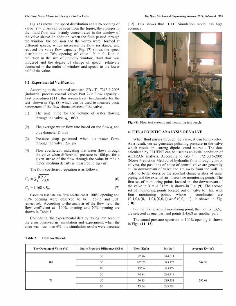
According to the national standard GB / T 17213.9-2005 (industrial process control valves Part 2-3: Flow capacity - Test procedures) [11], this research set benchmarks for the test shown in Fig. (8) which can be used to measure basic parameters of the flow characteristics of the valve .

(1) The unit time for the volume of water flowing through the valve. qv , m³/h

(2) The average water flow rate based on the flow qv and pipe diameter D, m/s

(3) Pressure drop generated when the water flows through the valve, !p , pa

(4) Flow coefficient, indicating that water flows through the valve when differential pressure is 100kpa, for a given stroke of the flow through the value in m³ / h meter, medium density is measured in kg / m³.

The flow coefficient equation is as follows:

CV =Q Gf!P (6)

CV = 1.168 ! KV (7)

Based on test data, the flow coefficient at 100% opening and 70% opening were observed to be 569.3 and 301, respectively. According to the analysis of the flow field, the flow coefficient at 100% opening and 70% opening are shown in Table 2. Comparing the experimental data by taking into account the error observed in simulation and experiment, when the error was less than 6%, the simulation results were accurate

[12]. This shows that CFD Simulation model has high accuracy.

Fig. (8). Flow test systems and measuring test bench.

4. THE ACOUSTIC ANALYSIS OF VALVE

When fluid passes through the valve, it can form vortex. As a result, vortex generates pulsating pressure in the valve which results in strong dipole sound source . The data calculated by FLUENT can be used as an initial condition of ACTRAN analysis. According to GB / T 17213.16-2005 (Noise Prediction Method of hydraulic flow through control valves), the positions of noise of control valve are generally at 1m downstream of valve and 1m away from the wall. In order to better describe the spectral characteristics of inner piping and the external air, it sets two monitoring points. The first set of monitoring points located in the downstream of the valve in X = -1.318m, is shown in Fig. (9). The second set of monitoring points located out of valve to 1m, with four monitoring points, whose coordinates are 0,1,0 , 0,−1,0 , 0,0,1 , !"# 0,0,−1 , is shown in Fig.

(10). For the first group of monitoring point, the points 1,3,5,7 are selected as one part and points 2,4,6,8 as another part. The sound pressure spectrum at 100% opening is shown in Figs. (11, 12).

Table 2. Flow coefficient.

The Opening of Valve (%) Static Pressure Difference (KPa) Flow (Kg/s) Kv (m3) Average Kv (m3)

100

30 82.86 544.611

544.39 50 107.20 545.773

80 135.6 545.779

70

30 44.84 294.719

292.68 50 56.83 289.331

80 73.04 293.980


It can be seen from Figs. (11, 12) that:

(a)

(b)

Fig. (9). Distribution of monitoring points in x=-1.1318m.

Fig. (10). Monitoring points outside the valve at 1m.

(1) When the frequency was less than 2500HZ, the distribution of sound pressure at different frequencies was observed to be similar. With increased frequency, the sound pressure distribution of different monitoring points showed huge difference and generated fluctuation and messy situation.

(2) Noise level of monitoring point within the valve substantially fluctuated between 20 to 140db. The band was wide and there was no obvious frequency. Thus, the noise of valve was observed to be a broadband noise.

(3) The amplitude of sound pressure and the range of fluctuations were relatively large when monitoring points were at low frequency. But with increasing frequency, amplitude and fluctuations decreased. It can be seen that the energy of noise at low frequency was observed to be higher than at high frequency.

As compared to the sound pressure spectrum at 70% opening (Figs. 13, 14), it can be seen that the fluctuation at 70% opening ranged between 40 to 160db, which was larger than 100% opening. The reason is that when the degree of opening of valve reduces, the turbulence intensity, speed and pressure fluctuations correspondingly increase, which leads to increase in the noise pressure amplitude. This was also observed in the analysis of flow field.

Fig. (11). Sound pressure spectrum of 100% opening.


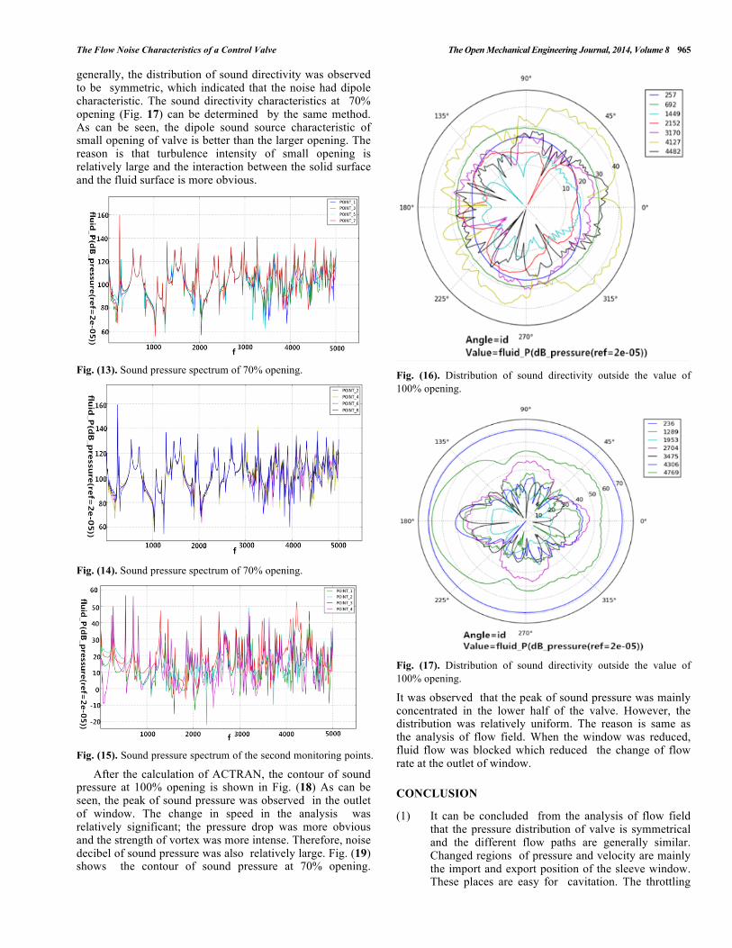
Similar to the above analysis, the pressure spectrum of second set of monitoring point is shown in Fig. (15). According to the acoustic pressure spectrum, it was observed that, when the frequency was approximately at 257Hz, 692Hz, 1449Hz, 2152Hz, 3170Hz, 4127Hz, and 4482Hz, the sound pressure was at the crest. Following this, the sound directivity characteristics of these frequencies are shown in Fig. (16). As can be seen from the figure, the sound directivity was observed to be regular and symmetrical, when the noise was at low frequencies. With increased frequency, the rule of sound directivity became worse. But


generally, the distribution of sound directivity was observed to be symmetric, which indicated that the noise had dipole characteristic. The sound directivity characteristics at 70% opening (Fig. 17) can be determined by the same method. As can be seen, the dipole sound source characteristic of small opening of valve is better than the larger opening. The reason is that turbulence intensity of small opening is relatively large and the interaction between the solid surface and the fluid surface is more obvious.



Fig. (15). Sound pressure spectrum of the second monitoring points.

After the calculation of ACTRAN, the contour of sound pressure at 100% opening is shown in Fig. (18) As can be seen, the peak of sound pressure was observed in the outlet of window. The change in speed in the analysis was relatively significant; the pressure drop was more obvious and the strength of vortex was more intense. Therefore, noise decibel of sound pressure was also relatively large. Fig. (19) shows the contour of sound pressure at 70% opening.

Fig. (16). Distribution of sound directivity outside the value of 100% opening.

Fig. (17). Distribution of sound directivity outside the value of 100% opening.

It was observed that the peak of sound pressure was mainly concentrated in the lower half of the valve. However, the distribution was relatively uniform. The reason is same as the analysis of flow field. When the window was reduced, fluid flow was blocked which reduced the change of flow rate at the outlet of window.

CONCLUSION

(1) It can be concluded from the analysis of flow field that the pressure distribution of valve is symmetrical and the different flow paths are generally similar. Changed regions of pressure and velocity are mainly the import and export position of the sleeve window. These places are easy for cavitation. The throttling


effect of the window increases the flow rate of the valve and the flow resistance, when the opening of valve is reduced.

Fig. (18). The contour of sound pressure of 100% opening.

Fig. (19). The contour of sound pressure of 70% opening.

(2) Observed by acoustic analysis, the fluctuation range of sound pressure and the energy of acoustic were relatively large when the noise was at low frequency. The sound pressure amplitude, the fluctuation range and energy were reduced when the noise was at high frequency.

(3) The distribution of sound directivity was observed to be symmetric and the noise of valve had dipole characteristic.

(4) When the opening of valve, turbulence intensity, velocity and pressure fluctuations increased, the amplitude of the sound pressure also increased correspondingly.

(5) When the speed of valve changed rapidly, the intensity of turbulent eddies was increased and the noise decibel of sound pressure correspondingly increased. In addition, the peak sound pressure was observed in the strongest areas of pressure drop.

CONFLICT OF INTEREST

The authors confirm that this article content has no conflicts of interest.

ACNOWLEDGEMENTS

This work was supported by the National Natural Science Foundation of China (NO.11472095).

REFERENCES

[1] Z. M. Wang, and H. J. Wei, “Valve noise in a lower fluid duct”, Journal of Acoustics, no. 6, pp. 437-443, 1991.

[2] C.W. Liu, Y. Li, X.Li, and J. Cao, “CFD analog-based valve flow noise simulation of gas pipline”, Gas Storage and Transportation, vol. 31, no. 9, pp. 657-662, 2012.

[3] S. G. Liu, H. Liu, H. Shu, D. Zhao, Z. Xu, and L. Zhang, “Flow noise reduction of outboard valves based on internal flow path optimization”, Journal of Harbin Engineering University, no. 34, pp. 511-516, 2013.

[4] M. J. Lighthill, “On Sound Generated Aerodynamically, IGeneral Theory”, Proceedings of the Royal Society, vol. 211, 1952.

[5] H. K. Versteeg, and W. Malalasekera, “An introduction to co-mputational fluid dynamics”, World Book Publishing Company : Harlow, 2000.

[6] M. B. B. D. R. Abbott, “Computational Fluid Dynamics-An Introduction for Engineers”, Longman Scientific & Technical : Harlow, England, 1989.

[7] L. J. Wang, “The theory and application of Large eddy simulation”, Journal of Hohai University, no. 3, pp. 261-265, 2004.

[8] H. Q. Wang, Z. Y. Wang, and G. X. Kou, “Theoretical Development and Application of Large Eddy Simulation in Engineering”, Journal of Fluid Machinery, no. 7, 2004.

[9] L.Y. Meng, C.-W. Liu, Y.-X. Li, W.-C. Wang, and F. Zhang, “Aero-acoustics generation mechanism and analysis methods for natural gas pipelines”, Journal of China University of Petroleum, no. 6, pp. 128-136, 2012.

[10] Y. Zhang, H.-P. Fu, and G.-P. Miao, “LES-Based Numerical Simulation of Flow Noise for Submerged Body with Cavities”, Journal of Shanghai Jiaotong University, no. 12, pp. 1868-1873, 2011.

[11] GB/T 17213.9, The experimental procedure of flow capacity, 2005. [12] Z. W. Song, “Numerical simulation of internal flow and test

research of cut-off valve”, Zhejiang Sci-Tech University, 2012.

Received: February 17, 2014 Revised: March 21, 2015 Accepted: June 9, 2015 © Nie et al.; Licensee Bentham Open

This is an open access article licensed under the terms of the (https://creativecommons.org/licenses/by/4.0/legalcode), which permits unrestricted, non-commercial use, distribution and reproduction in any medium, provided the work is properly cited.

960 the open mechanical engineering journal, … · 960 the open mechanical engineering journal ......

Documents