9780199554232 000i-00ii sodhi biology color htitle 1. · only in small ways, most individuals...

CHAP T E R 2

BiodiversityKevin J. Gaston

Biological diversity or biodiversity (the latter termis simply a contraction of the former) is the variety oflife, in all of its many manifestations. It is a broadunifying concept, encompassing all forms, levelsand combinations of natural variation, at all levelsof biological organization (Gaston and Spicer2004). A rather longer and more formal definitionis given in the international Convention onBiological Diversity (CBD; the definition isprovided in Article 2), which states that“‘Biological diversity’ means the variabilityamong living organisms from all sources includ-ing, inter alia, terrestrial, marine and other aquaticecosystems and the ecological complexes of whichthey are part; this includes diversitywithin species,between species and of ecosystems”. Whicheverdefinition is preferred, one can, for example,speak equally of the biodiversity of some givenarea or volume (be it large or small) of the land orsea, of the biodiversity of a continent or an oceanbasin, or of the biodiversity of the entire Earth.Likewise, one can speak of biodiversity at present,at a given time or period in the past or in the future,or over the entire history of life on Earth.

The scale of the variety of life is difficult, andperhaps impossible, for any of us truly to visua-lize or comprehend. In this chapter I first attemptto give some sense of the magnitude of biodiver-sity by distinguishing between different key ele-ments and what is known about their variation.Second, I consider how the variety of life haschanged through time, and third and finallyhow it varies in space. In short, the chapter will,inevitably in highly summarized form, addressthe three key issues of how much biodiversitythere is, how it arose, and where it can be found.

2.1 How much biodiversity is there?

Some understanding of what the variety of lifecomprises can be obtained by distinguishing be-tween different key elements. These are the basicbuilding blocks of biodiversity. For convenience,they can be divided into three groups: geneticdiversity, organismal diversity, and ecologicaldiversity (Table 2.1). Within each, the elementsare organized in nested hierarchies, with thosehigher order elements comprising lower order

Table 2.1 Elements of biodiversity (focusing on those levels that are most commonly used). Modified from Heywood and Baste(1995).

Ecological diversity Organismal diversity

Biogeographic realms Domains or KingdomsBiomes PhylaProvinces FamiliesEcoregions GeneraEcosystems SpeciesHabitats Genetic diversity Subspecies

Populations Populations PopulationsIndividuals Individuals

ChromosomesGenes

Nucleotides

27

1

© Oxford University Press 2010. All rights reserved. For permissions please email: [email protected]

ones. The three groups are intimately linked andshare some elements in common.

2.1.1 Genetic diversity

Genetic diversity encompasses the components ofthe genetic coding that structures organisms (nu-cleotides, genes, chromosomes) and variation inthe genetic make-up between individuals within apopulation and between populations. This is theraw material on which evolutionary processes act.Perhaps themostbasicmeasure of genetic diversityis genome size—the amount of DNA (Deoxyribo-nucleic acid) inone copyof a species’ chromosomes(also called the C-value). This can vary enormous-ly,withpublished eukaryote genome sizes rangingbetween 0.0023 pg (picograms) in the parasitic mi-crosporidium Encephalitozoon intestinalis and 1400pg in the free-living amoeba Chaos chaos (Gregory2008). These translate into estimates of 2.2 millionand 1369 billion base pairs (the nucleotides on op-posing DNA strands), respectively. Thus, even atthis level the scale of biodiversity is daunting. Cellsize tends to increase with genome size. Humanshave a genome size of 3.5 pg (3.4 billion base pairs).

Much of genome size comprises non-codingDNA, and there is usually no correlation betweengenome size and the number of genes coded. Thegenomes of more than 180 species have beencompletely sequenced and it is estimated that, forexample, there are around 1750 genes for the bacte-ria Haemophilus influenzae and 3200 for Escherichiacoli, 6000 for theyeastSaccharomyces cerevisiae, 19000for the nematode Caenorhabditis elegans, 13 500 forthe fruit flyDrosophila melanogaster, and�25 000 fortheplantArabidopsis thaliana, themouseMusmuscu-lus, brown rat Rattus norvegicus and human Homosapiens. There is strong conservatism of some genesacrossmuchof thediversityof life.Thedifferences ingenetic compositionof species giveus indications oftheir relatedness, and thus important informationasto how the history and variety of life developed.

Genes are packaged into chromosomes. Thenumber of chromosomes per somatic cell thusfar observed varies between 2 for the jumper antMyrmecia pilosula and 1260 for the adders-tonguefern Ophioglossum reticulatum. The ant species re-produces by haplodiploidy, in which fertilized

eggs (diploid) develop into females and unfertil-ized eggs (haploid) become males, hence the lat-ter have the minimal achievable singlechromosome in their cells (Gould 1991). Humanshave 46 chromosomes (22 pairs of autosomes,and one pair of sex chromosomes).

Within a species, genetic diversity is commonlymeasured in terms of allelic diversity (averagenumber of alleles per locus), gene diversity (het-erozygosity across loci), or nucleotide differences.Large populations tend to have more genetic di-versity than small ones, more stable populationsmore than those that wildly fluctuate, and popu-lations at the center of a species’ geographic rangeoften have more genetic diversity than those atthe periphery. Such variation can have a varietyof population-level influences, including on pro-ductivity/biomass, fitness components, behav-ior, and responses to disturbance, as well asinfluences on species diversity and ecosystemprocesses (Hughes et al. 2008).

2.1.2 Organismal diversity

Organismal diversity encompasses the full taxo-nomic hierarchy and its components, from indi-viduals upwards to populations, subspecies andspecies, genera, families, phyla, and beyond tokingdoms and domains. Measures of organismaldiversity thus include some of the most familiarexpressions of biodiversity, such as the numbersof species (i.e. species richness). Others should bebetter studied and more routinely employed thanthey have been thus far.

Starting at the lowest level of organismal diver-sity, little is known about how many individualorganisms there are at any one time, although thisis arguably an important measure of the quantityand variety of life (given that, even if sometimesonly in small ways, most individuals differ fromone another). Nonetheless, the numbers must beextraordinary. The global number of prokaryoteshas been estimated to be 4–6 x 1030 cells—manymillion times more than there are stars in thevisible universe (Copley 2002)—with a produc-tion rate of 1.7 x 1030 cells per annum (Whitman etal. 1998). The numbers of protists is estimated at104�107 individuals per m2 (Finlay 2004).

28 CONSERVATION BIOLOGY FOR ALL

Sodhi and Ehrlich: Conservation Biology for All. http://ukcatalogue.oup.com/product/9780199554249.do


Impoverished habitats have been estimated tohave 105 individual nematodes per m2, andmore productive habitats 106�107 per m2, possi-bly with an upper limit of 108 per m2; 1019 hasbeen suggested as a conservative estimate of theglobal number of individuals of free-living nema-todes (Lambshead 2004). By contrast, it hasbeen estimated that globally there may be less than1011 breeding birds at any one time, fewer than 17for every person on the planet (Gaston et al. 2003).

Individual organisms can be grouped into rela-tively independent populations of a species on thebasis of limited gene flow and some level of genet-ic differentiation (as well as on ecological criteria).The population is a particularly important ele-ment of biodiversity. First, it provides an impor-tant link between the different groups of elementsof biodiversity (Table 2.1). Second, it is the scale atwhich it is perhaps most sensible to consider lin-kages between biodiversity and the provision ofecosystem services (supporting services—e.g. nu-trient cycling, soil formation, primary production;provisioning services—e.g. food, freshwater,timber and fiber, fuel; regulating services—e.g.climate regulation, flood regulation, disease regu-lation, water purification; cultural services—e.g.aesthetic, spiritual, educational, recreational;MEA 2005). Estimates of the density of such po-pulations and the average geographic range sizesof species suggest a total of about 220 distinctpopulations per eukaryote species (Hughes et al.1997). Multiplying this by a range of estimates ofthe extant numbers of species, gives a global totalof 1.1 to 6.6 x 109 populations (Hughes et al. 1997),one or fewer for every person on the planet. Theaccuracy of this figure is essentially unknown,with major uncertainties at each step of the calcu-lation, but the ease withwhich populations can beeradicated (e.g. through habitat destruction) sug-gests that the total is being eroded at a rapid rate.

People have long pondered one of the impor-tant contributors to the calculation of the totalnumber of populations, namely howmany differ-ent species of organisms there might be. Greatestuncertainty continues to surround the richness ofprokaryotes, and in consequence they are oftenignored in global totals of species numbers. Thisis in part variously because of difficulties in ap-

plying standard species concepts, in culturing thevast majority of these organisms and thereby ap-plying classical identification techniques, and bythe vast numbers of individuals. Indeed, depend-ing on the approach taken, the numbers of pro-karyotic species estimated to occur even in verysmall areas can vary by a few orders of magni-tude (Curtis et al. 2002; Ward 2002). The rate ofreassociation of denatured (i.e. single stranded)DNA has revealed that in pristine soils and sedi-ments with high organic content samples of 30 to100 cm3 correspond to c. 3000 to 11 000 differentgenomes, and may contain 104 different prokary-otic species of equivalent abundances (Torsviket al. 2002). Samples from the intestinal microbialflora of just three adult humans contained repre-sentatives of 395 bacterial operational taxonomicunits (groups without formal designation of tax-onomic rank, but thought here to be roughlyequivalent to species), of which 244 were previ-ously unknown, and 80% were from species thathave not been cultured (Eckburg et al. 2005). Like-wise, samples from leaves were estimated to har-bor at least 95 to 671 bacterial species from each ofnine tropical tree species, with only 0.5% com-mon to all the tree species, and almost all of thebacterial species being undescribed (Lambaiset al. 2006). On the basis of such findings, globalprokaryote diversity has been argued to comprisepossibly millions of species, and some have sug-gested it may be many orders of magnitude morethan that (Fuhrman and Campbell 1998; Dykhui-zen 1998; Torsvik et al. 2002; Venter et al. 2004).

Although much more certainty surrounds es-timates of the numbers of eukaryotic than pro-karyotic species, this is true only in a relative andnot an absolute sense. Numbers of eukaryoticspecies are still poorly understood. A wide vari-ety of approaches have been employed to esti-mate the global numbers in large taxonomicgroups and, by summation of these estimates,how many extant species there are overall.These approaches include extrapolations basedon counting species, canvassing taxonomic ex-perts, temporal patterns of species description,proportions of undescribed species in samples,well-studied areas, well-studied groups, species-abundance distributions, species-body size

BIODIVERSITY 29

1


distributions, and trophic relations (Gaston2008). One recent summary for eukaryotesgives lower and upper estimates of 3.5 and 108million species, respectively, and a working fig-ure of around 8 million species (Table 2.2). Basedon current information the two extremes seemrather unlikely, but the working figure at leastseems tenable. However, major uncertaintiessurround global numbers of eukaryotic speciesin particular environments which have beenpoorly sampled (e.g. deep sea, soils, tropicalforest canopies), in higher taxa which are ex-tremely species rich or with species which arevery difficult to discriminate (e.g. nematodes,arthropods), and in particular functional groupswhich are less readily studied (e.g. parasites). Awide array of techniques is now being employedto gain access to some of the environments thathave been less well explored, including ropeclimbing techniques, aerial walkways, cranesand balloons for tropical forest canopies, andremotely operated vehicles, bottom landers, sub-marines, sonar, and video for the deep ocean.Molecular and better imaging techniques arealso improving species discrimination. Perhapsmost significantly, however, it seems highlyprobable that the majority of species are para-sites, and yet few people tend to think aboutbiodiversity from this viewpoint.

Howmany of the total numbers of species havebeen taxonomically described remains surpris-ingly uncertain, in the continued absence of a

single unified, complete andmaintained databaseof valid formal names. However, probably about2 million extant species are regarded as beingknown to science (MEA 2005). Importantly, thistotal hides two kinds of error. First, there areinstances in which the same species is knownunder more than one name (synonymy). This ismore frequent amongst widespread species,which may show marked geographic variationin morphology, and may be described anew re-peatedly in different regions. Second, one namemay actually encompass multiple species (hom-onymy). This typically occurs because these spe-cies are very closely related, and look very similar(cryptic species), and molecular analyses may berequired to recognize or confirm their differences.Levels of as yet unresolved synonymy are un-doubtedly high in many taxonomic groups. In-deed, the actual levels have proven to be a keyissue in, for example, attempts to estimate theglobal species richness of plants, with the highlyvariable synonymy rate amongst the few groupsthat have been well studied in this regard makingdifficult the assessment of the overall level ofsynonymy across all the known species. Equally,however, it is apparent that cryptic speciesabound, with, for example, one species of neo-tropical skipper butterfly recently having beenshown actually to be a complex of ten species(Hebert et al. 2004).

New species are being described at a rateof about 13 000 per annum (Hawksworth and

Table 2.2 Estimates (in thousands), by different taxonomic groups, of the overall global numbers of extant eukaryotespecies. Modified from Hawksworth and Kalin‐Arroyo (1995) and May (2000).

Overall species

High Low Working figure Accuracy of working figure

‘Protozoa’ 200 60 100 very poor‘Algae’ 1000 150 300 very poorPlants 500 300 320 goodFungi 2700 200 1500 moderateNematodes 1000 100 500 very poorArthropods 101 200 2375 4650 moderateMolluscs 200 100 120 moderateChordates 55 50 50 goodOthers 800 200 250 moderate

Totals 107 655 3535 7790 very poor




Kalin-Arroyo 1995), or about 36 species on theaverage day. Given even the lower estimates ofoverall species numbers this means that there islittle immediate prospect of greatly reducing thenumbers that remain unknown to science. This isparticularly problematic because the describedspecies are a highly biased sample of the extantbiota rather than the random one that might en-able more ready extrapolation of its properties toall extant species. On average, described speciestend to be larger bodied, more abundant andmore widespread, and disproportionately fromtemperate regions. Nonetheless, new species con-tinue to be discovered in even otherwise relative-ly well-known taxonomic groups. New extantfish species are described at the rate of about130–160 each year (Berra 1997), amphibian spe-cies at about 95 each year (from data in Frost2004), bird species at about 6–7 each year (VanRootselaar 1999, 2002), and terrestrial mammalsat 25–30 each year (Ceballos and Ehrlich 2009).Recently discovered mammals include marsu-pials, whales and dolphins, a sloth, an elephant,primates, rodents, bats and ungulates.

Given the high proportion of species that haveyet to be discovered, it seems highly likely thatthere are entire major taxonomic groups of organ-isms still to be found. That is, new examples ofhigher level elements of organismal diversity.This is supported by recent discoveries of possi-ble new phyla (e.g. Nanoarchaeota), new orders(e.g. Mantophasmatodea), new families (e.g. As-pidytidae) and new subfamilies (e.g. Martiali-nae). Discoveries at the highest taxonomic levelshave particularly served to highlight the muchgreater phyletic diversity of microorganismscompared with macroorganisms. Under one clas-sification 60% of living phyla consist entirely orlargely of unicellular species (Cavalier-Smith2004). Again, this perspective on the variety oflife is not well reflected in much of the literatureon biodiversity.

2.1.3 Ecological diversity

The third group of elements of biodiversity en-compasses the scales of ecological differencesfrom populations, through habitats, to ecosys-

tems, ecoregions, provinces, and on up to biomesand biogeographic realms (Table 2.1). This is animportant dimension to biodiversity not readilycaptured by genetic or organismal diversity, andin many ways is that which is most immediatelyapparent to us, giving the structure of the naturaland semi-natural world in which we live. How-ever, ecological diversity is arguably also the leastsatisfactory of the groups of elements of biodiver-sity. There are two reasons. First, whilst theseelements clearly constitute useful ways of break-ing up continua of phenomena, they are difficultto distinguish without recourse to what ultimate-ly constitute some essentially arbitrary rules. Forexample, whilst it is helpful to be able to labeldifferent habitat types, it is not always obviousprecisely where one should end and anotherbegin, because no such beginnings and endingsreally exist. In consequence, numerous schemeshave been developed for distinguishing betweenmany elements of ecological diversity, often withwide variation in the numbers of entities recog-nized for a given element. Second, some of theelements of ecological diversity clearly have bothabiotic and biotic components (e.g. ecosystems,ecoregions, biomes), and yet biodiversity is de-fined as the variety of life.

Much recent interest has focused particularlyon delineating ecoregions and biomes, principal-ly for the purposes of spatial conservationplanning (see Chapter 11), and there has thusbeen a growing sense of standardization of theschemes used. Ecoregions are large areal unitscontaining geographically distinct species as-semblages and experiencing geographically dis-tinct environmental conditions. Carefulmapping schemes have identified 867 terrestrialecoregions (Figure 2.1 and Plate 1; Olson et al.2001), 426 freshwater ecoregions (Abell et al.2008), and 232 marine coastal & shelf area ecor-egions (Spalding et al. 2007). Ecoregions can inturn be grouped into biomes, global-scale bio-geographic regions distinguished by unique col-lections of species assemblages and ecosystems.Olson et al. (2001) distinguish 14 terrestrialbiomes, some of which at least will be very fa-miliar wherever in the world one resides (tropi-cal & subtropical moist broadleaf forests;

BIODIVERSITY 31

1


tropical & subtropical dry broadleaf forests;tropical & subtropical coniferous forests; tem-perate broadleaf & mixed forests; temperate co-niferous forests; boreal forest/taiga; tropical &subtropical grasslands, savannas & shrublands;temperate grasslands, savannas & shrublands;flooded grasslands & savannas; montane grass-lands & shrublands; tundra; Mediterranean for-ests, woodlands & scrub; deserts & xericshrublands; mangroves).

At a yet coarser spatial resolution, terrestrialand aquatic systems can be divided into bio-geographic realms. Terrestrially, eight suchrealms are typically recognized, Australasia,Antarctic, Afrotropic, Indo-Malaya, Nearctic,Neotropic, Oceania and Palearctic (Olson et al.2001). Marine coastal & shelf areas have beendivided into 12 realms (Arctic, TemperateNorth Atlantic, Temperate Northern Pacific,Tropical Atlantic, Western Indo-Pacific, CentralIndo-Pacific, Eastern Indo-Pacific, TropicalEastern Pacific, Temperate South America,Temperate Southern Africa, Temperate Austra-lasia, and Southern Ocean; Spalding et al.2007). There is no strictly equivalent schemefor the pelagic open ocean, although one hasdivided the oceans into four primary units (Polar,

Westerlies, Trades and Coastal boundary), whichare then subdivided, on the basis principallyof biogeochemical features, into a further 12biomes (Antarctic Polar, Antarctic WesterlyWinds, Atlantic Coastal, Atlantic Polar, AtlanticTrade Wind, Atlantic Westerly Winds, IndianOcean Coastal, Indian Ocean Trade Wind, PacificCoastal, Pacific Polar, Pacific Trade Wind, PacificWesterly Winds), and then into a finer 51 units(Longhurst 1998).

2.1.4 Measuring biodiversity

Given the multiple dimensions and the complex-ity of the variety of life, it should be obvious thatthere can be no single measure of biodiversity(see Chapter 16). Analyses and discussions ofbiodiversity have almost invariably to be framedin terms of particular elements or groups of ele-ments, although this may not always be apparentfrom the terminology being employed (the term‘biodiversity’ is used widely and without explicitqualification to refer to only some subset of thevariety of life). Moreover, they have to be framedin terms either of “number” or of “heterogeneity”measures of biodiversity, with the former disre-garding the degrees of difference between the

Figure 2.1 The terrestrial ecoregions. Reprinted from Olson et al. (2001).




occurrences of an element of biodiversity and thelatter explicitly incorporating such differences.For example, organismal diversity could be ex-pressed in terms of species richness, which is anumber measure, or using an index of diversitythat incorporates differences in the abundances ofthe species, which is a heterogeneity measure.The two approaches constitute different re-sponses to the question of whether biodiversityis similar or different in an assemblage in which asmall proportion of the species comprise most ofthe individuals, and therefore would predomi-nantly be obtained in a small sample of indivi-duals, or in an assemblage of the same totalnumber of species in which abundances aremore evenly distributed, and thus more specieswould occur in a small sample of individuals(Purvis and Hector 2000). The distinction be-tween number and heterogeneity measures isalso captured in answers to questions that reflecttaxonomic heterogeneity, for examplewhether theabove-mentioned group of 10 skipper butterfliesis as biodiverse as a group of five skipper speciesand five swallowtail species (e.g. Hendricksonand Ehrlich 1971).

In practice, biodiversity tends most commonlyto be expressed in terms of number measures oforganismal diversity, often the numbers of a giventaxonomic level, and particularly the numbers ofspecies. This is in large part a pragmatic choice.Organismal diversity is better documented andoftenmore readily estimated than is genetic diver-sity, and more finely and consistently resolvedthan much of ecological diversity. Organismaldiversity, however, is problematic inasmuch asthe majority of it remains unknown (and thusstudies have to be based on subsets), and preciselyhow naturally and well many taxonomic groupsare themselves delimited remains in dispute.Perhaps most importantly it also remains butone, and arguably a quite narrow, perspective onbiodiversity.

Whilst accepting the limitations of measuringbiodiversity principally in terms of organismaldiversity, the following sections on temporaland spatial variation in biodiversity will followthis course, focusing in many cases on speciesrichness.

2.2 How has biodiversity changedthrough time?

The Earth is estimated to have formed, by theaccretion through large and violent impacts ofnumerous bodies, approximately 4.5 billionyears ago (Ga). Traditionally, habitable worldsare considered to be those on which liquidwater is stable at the surface. On Earth, both theatmosphere and the oceans maywell have startedto form as the planet itself did so. Certainly, life isthought to have originated on Earth quite early inits history, probably after about 3.8–4.0 Ga, whenimpacts from large bodies from space are likely tohave declined or ceased. It may have originatedin a shallow marine pool, experiencing intenseradiation, or possibly in the environment of adeeper water hydrothermal vent. Because of thesubsequent recrystallisation and deformation ofthe oldest sediments on Earth, evidence for earlylife must be found in its metabolic interactionwith the environment. The earliest, and highlycontroversial, evidence of life, from such indirectgeochemical data, is from more than 3.83 billionyears ago (Dauphas et al. 2004). Relatively unam-biguous fossil evidence of life dates to 2.7 Ga(López-García et al. 2006). Either way, life hasthus been present throughout much of the Earth’sexistence. Although inevitably attention tends tofall on more immediate concerns, it is perhapsworth occasionally recalling this deep heritage inthe face of the conservation challenges of today.For much of this time, however, life comprisedPrecambrian chemosynthetic and photosyntheticprokaryotes, with oxygen-producing cyanobac-teria being particularly important (Labandeira2005). Indeed, the evolution of oxygenic photo-synthesis, followed by oxygen becoming a majorcomponent of the atmosphere, brought about adramatic transformation of the environmenton Earth. Geochemical data has been argued tosuggest that oxygenic photosynthesis evolvedbefore 3.7 Ga (Rosing and Frei 2004), althoughothers have proposed that it could not have arisenbefore c.2.9 Ga (Kopp et al. 2005).

These cyanobacteria were initially responsiblefor the accumulation of atmospheric oxygen. Thisin turn enabled the emergence of aerobically

BIODIVERSITY 33

1


metabolizing eukaryotes. At an early stage, eu-karyotes incorporated within their structure aer-obically metabolizing bacteria, giving rise toeukaryotic cells with mitochondria; all anaerobi-cally metabolizing eukaryotes that have beenstudied in detail have thus far been found tohave had aerobic ancestors, making it highlylikely that the ancestral eukaryote was aerobic(Cavalier-Smith 2004). This was a fundamentallyimportant event, leading to heterotrophic micro-organisms and sexual means of reproduction.Such endosymbiosis occurred serially, by simplerand more complex routes, enabling eukaryotes todiversify in a variety of ways. Thus, the inclusionof photosynthesizing cyanobacteria into a eu-karyote cell that already contained a mitochon-drion gave rise to eukaryotic cells with plastidsand capable of photosynthesis. This event alonewould lead to dramatic alterations in the Earth’secosystems.

Precisely when eukaryotes originated, whenthey diversified, and how congruent was thediversification of different groups remains un-clear, with analyses giving a very wide range ofdates (Simpson and Roger 2004). The uncertainty,which is particularly acute when attempting tounderstand evolutionary events in deep time, re-sults principally from the inadequacy of the fossilrecord (which, because of the low probabilities offossilization and fossil recovery, will always tendto underestimate the ages of taxa) and the diffi-culties of correctly calibrating molecular clocks soas to use the information embodied in geneticsequences to date these events. Nonetheless,there is increasing convergence on the idea thatmost known eukaryotes can be placed in one offive or six major clades—Unikonts (Opisthokontsand Amoebozoa), Plantae, Chromalveolates, Rhi-zaria and Excavata (Keeling et al. 2005; Roger andHug 2006).

Focusing on the last 600 million years, attentionshifts somewhat from the timing of key diversifi-cation events (which becomes less controversial)to how diversity per se has changed through time(which becomes more measurable). Arguably thecritical issue is how well the known fossil recordreflects the actual patterns of change that tookplace and how this record can best be analyzed

to address its associated biases to determine thoseactual patterns. The best fossil data are for marineinvertebrates and it was long thought that theseprincipally demonstrated a dramatic rise in diver-sity, albeit punctuated by significant periods ofstasis and mass extinction events. However, ana-lyses based on standardized sampling havemarkedly altered this picture (Figure 2.2). Theyidentify the key features of change in the numbersof genera (widely assumed to correlate with spe-cies richness) as comprising: (i) a rise in richnessfrom the Cambrian through to the mid-Devonian(�525–400 million years ago, Ma); (ii) a largeextinction in the mid-Devonian with no clear re-covery until the Permian (�400–300 Ma); (iii) alarge extinction in the late-Permian and again inthe late-Triassic (�250–200 Ma); and (iv) a rise inrichness through the late-Triassic to the present(�200–0 Ma; Alroy et al. 2008).

Whatever the detailed pattern of change in di-versity through time, most of the species thathave ever existed are extinct. Across a variety ofgroups (both terrestrial and marine), the bestpresent estimate based on fossil evidence is thatthe average species has had a lifespan (from itsappearance in the fossil record until the time itdisappeared) of perhaps around 1–10 Myr(McKinney 1997; May 2000). However, the varia-bility both within and between groups is verymarked, making estimation of what is the overallaverage difficult. The longest-lived species that iswell documented is a bryozoan that persistedfrom the early Cretaceous to the present, a periodof approximately 85 million years (May 2000). Ifthe fossil record spans 600 million years, totalspecies numbers were to have been roughly con-stant over this period, and the average life span ofindividual species were 1–10 million years, thenat any specific instant the extant species wouldhave represented 0.2–2% of those that have everlived (May 2000). If this were true of the presenttime then, if the number of extant eukaryote spe-cies numbers 8 million, 400 million might oncehave existed.

The frequency distribution of the numbers oftime periods with different levels of extinction ismarkedly right-skewed, with most periods hav-ing relatively low levels of extinction and a




minority having very high levels (Raup 1994).The latter are the periods of mass extinctionwhen 75–95% of species that were extant are es-timated to have become extinct. Their signifi-cance lies not, however, in the overall numbersof extinctions for which they account (over thelast 500 Myr this has been rather small), but in thehugely disruptive effect they have had on thedevelopment of biodiversity. Clearly neither ter-restrial nor marine biotas are infinitely resilient toenvironmental stresses. Rather, when pushed be-yond their limits they can experience dramaticcollapses in genetic, organismal and ecologicaldiversity (Erwin 2008). This is highly significantgiven the intensity and range of pressures thathave been exerted on biodiversity by humankind,and which have drastically reshaped the naturalworld over a sufficiently long period in respect toavailable data that we have rather little concept ofwhat a truly natural system should look like(Jackson 2008). Recovery from past mass extinc-tion events has invariably taken place. But, whilstthis may have been rapid in geological terms, ithas nonetheless taken of the order of a few mil-

lion years (Erwin 1998), and the resultant assem-blages have invariably had a markedly differentcomposition from those that preceded a massextinction, with groups which were previouslyhighly successful in terms of species richnessbeing lost entirely or persisting at reducednumbers.

2.3 Where is biodiversity?

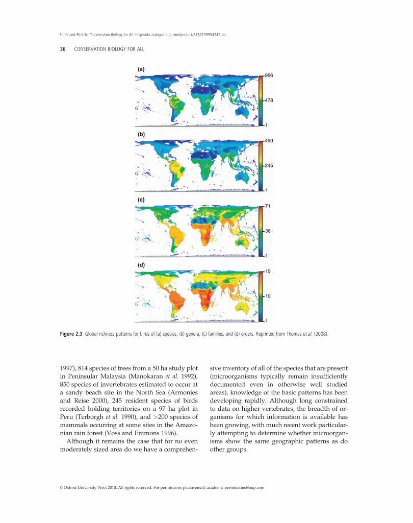
Just as biodiversity has varied markedly throughtime, so it also varies across space. Indeed, onecan think of it as forming a richly textured landand seascape, with peaks (hotspots) and troughs(coldspots), and extensive plains in between (Fig-ure 2.3 and Plate 2, and 2.4 and Plate 3; Gaston2000). Even locally, and just for particular groups,the numbers of species can be impressive, withfor example c.900 species of fungal fruiting bodiesrecorded from 13 plots totaling just 14.7 ha (hect-are) near Vienna, Austria (Straatsma and Krisai-Greilhuber 2003), 173 species of lichens on asingle tree in Papua New Guinea (Aptroot

500

0

200

400

Num

ber

of g

ener

a

600

800

Cm O S D C P Tr J K Pg Ng

400 300

Time (Ma)

200 100 0

Figure 2.2 Changes in generic richness of marine invertebrates over the last 600 million years based on a sampling‐standardized analysis of the fossilrecord. Ma, million years ago. Reprinted from Alroy et al. (2008) with permission from AAAS (American Association for the Advancement of Science).

BIODIVERSITY 35

1


1997), 814 species of trees from a 50 ha study plotin Peninsular Malaysia (Manokaran et al. 1992),850 species of invertebrates estimated to occur ata sandy beach site in the North Sea (Armoniesand Reise 2000), 245 resident species of birdsrecorded holding territories on a 97 ha plot inPeru (Terborgh et al. 1990), and >200 species ofmammals occurring at some sites in the Amazo-nian rain forest (Voss and Emmons 1996).

Although it remains the case that for no evenmoderately sized area do we have a comprehen-

sive inventory of all of the species that are present(microorganisms typically remain insufficientlydocumented even in otherwise well studiedareas), knowledge of the basic patterns has beendeveloping rapidly. Although long constrainedto data on higher vertebrates, the breadth of or-ganisms for which information is available hasbeen growing, with much recent work particular-ly attempting to determine whether microorgan-isms show the same geographic patterns as doother groups.

Figure 2.3 Global richness patterns for birds of (a) species, (b) genera, (c) families, and (d) orders. Reprinted from Thomas et al. (2008).




2.3.1 Land and water

The oceans cover �340.1 million km2 (67%), theland �170.3 million km2 (33%), and freshwaters(lakes and rivers) �1.5 million km2 (0.3%; withanother 16 million km2 under ice and permanentsnow, and 2.6 million km2 as wetlands, soil waterand permafrost) of the Earth’s surface. It wouldtherefore seem reasonable to predict that theoceans would be most biodiverse, followed bythe land and then freshwaters. In terms of num-bers of higher taxa, there is indeed some evidencethat marine systems are especially diverse. Forexample, of the 96 phyla recognized by Margulisand Schwartz (1998), about 69 have marine repre-sentatives, 55 have terrestrial ones, and 60 havefreshwater representatives. However, of the spe-cies described to date only about 15% are marineand 6% are freshwater. The fact that life began inthe sea seems likely to have played an importantrole in explaining why there are larger numbersof higher taxa in marine systems than in terrestri-al ones. The heterogeneity and fragmentation ofthe land masses (particularly that associatedwith the breakup of the “supercontinent” of

Gondwana from �180 Ma) is important in ex-plaining why there are more species in terrestrialsystems than in marine ones. Finally, the extremefragmentation and isolation of freshwater bodiesseems key to why these are so diverse for theirarea.

2.3.2 Biogeographic realms and ecoregions

Of the terrestrial realms, the Neotropics is gener-ally regarded as overall being the most biodi-verse, followed by the Afrotropics and Indo-Malaya, although the precise ranking of thesetropical regions depends on the way in whichorganismal diversity is measured. For example,for species the richest realm is the Neotropics foramphibians, reptiles, birds and mammals, but forfamilies it is the Afrotropics for amphibians andmammals, the Neotropics for reptiles, and theIndo-Malayan for birds (MEA 2005). In parts,these differences reflect variation in the historiesof the realms (especially mountain uplift and cli-mate changes) and the interaction with the emer-gence and spread of the groups, albeit perhaps

Figure 2.4 Global species richness patterns of birds, mammals, and amphibians, for total, rare (those in the lower quartile of range size for eachgroup) and threatened (according to the IUCN criteria) species. Reprinted from Grenyer et al. (2006).

BIODIVERSITY 37

1


complicated by issues of geographic consistencyin the definition of higher taxonomic groupings.

The Western Indo-Pacific and CentralIndo-Pacific realms have been argued to be acenter for the evolutionary radiation of manygroups, and are thought to be perhaps the globalhotspot of marine species richness and endemism(Briggs 1999; Roberts et al. 2002). With a shelf areaof 6 570 000 km2, which is considered to be asignificant influence, it has more than 6000 spe-cies of molluscs, 800 species of echinoderms, 500species of hermatypic (reef forming) corals, and4000 species of fish (Briggs 1999).

At the scale of terrestrial ecoregions, the mostspeciose for amphibians and reptiles are in theNeotropics, for birds in Indo-Malaya, Neotropicsand Afrotropics, and for mammals in the Neo-tropics, Indo-Malaya, Nearctic, and Afrotropics(Table 2.3). Amongst the freshwater ecoregions,those with globally high richness of freshwaterfish include the Brahmaputra, Ganges, andYangtze basins in Asia, and large portions ofthe Mekong, Chao Phraya, and Sitang and Irra-waddy; the lower Guinea in Africa; and theParaná and Orinoco in South America (Abellet al. 2008).

2.3.3 Latitude

Perhaps the best known of all spatial patterns inbiodiversity is the general increase in species

richness (and some other elements of organismaldiversity) towards lower (tropical) latitudes.Several features of this gradient are of note:(i) it is exhibited in marine, terrestrial and fresh-waters, and by virtually all major taxonomicgroups, including microbes, plants, invertebratesand vertebrates (Hillebrand 2004; Fuhrman et al.2008); (ii) it is typically manifest whether biodi-versity is determined at local sites, across largeregions, or across entire latitudinal bands; (iii) ithas been a persistent feature of much of thehistory of life on Earth (Crane and Lidgard1989; Alroy et al. 2008); (iv) the peak of diversityis seldom at the equator itself, but seems often tobe displaced somewhat further north (often at�20–30�N); (v) it is commonly, though far fromuniversally, asymmetrical about the equator, in-creasing rapidly from northern regions to theequator and declining slowly from the equatorto southern regions; and (vi) it varies markedlyin steepness for different major taxonomicgroups with, for example, butterflies beingmore tropical than birds.

Although it attracts much attention in its ownright, it is important to see the latitudinal patternin species richness as a component of broaderspatial patterns of richness. As such, the mechan-isms that give rise to it are also those that give riseto those broader patterns. Ultimately, higher spe-cies richness has to be generated by some combi-nation of greater levels of speciation (a cradle of

Table 2.3 The five most species rich terrestrial ecoregions for each of four vertebrate groups. AT – Afrotropic, IM – Indo‐Malaya,NA – Nearctic, and NT–Neotropic. Data from Olson et al. (2001).

Amphibians Reptiles Birds Mammals

1 Northwestern Andeanmontane forests(NT)

Peten‐Veracruzmoist forests (NT)

Northern Indochinasubtropical forests (IM)

Sierra Madre de Oaxacapine‐oak forests (NT)

2 Eastern Cordillera realmontane forests(NT)

Southwest Amazonmoist forests (NT)

Southwest Amazon moistforests (NT)

Northern Indochinasubtropical forests(IM)

3 Napomoist forests (NT) Napo moist forests(NT)

Albertine Rift montaneforests (AT)

Sierra Madre Orientalpine‐oak forests (NA)

4 Southwest Amazonmoist forests (NT)

Southern Pacific dryforests (NT)

Central Zambezian Miombowoodlands (AT)

Southwest Amazonmoist forests (NT)

5 Choco‐Darien moistforests (NT)

Central Americanpine‐oak forests(NT)

Northern Acacia‐Commiphora bushlands &thickets (AT)

Central ZambezianMiombo woodlands(AT)




diversity), lower levels of extinction (a museumof diversity) or greater net movements of geo-graphic ranges. It is likely that their relative im-portance in giving rise to latitudinal gradientsvaries with taxon and region. This said, greaterlevels of speciation at low latitudes and rangeexpansion of lineages from lower to higherlatitudes seem to be particularly important(Jablonski et al. 2006; Martin et al. 2007). Moreproximally, key constraints on speciation and ex-tinction rates and range movements are thoughtto be levels of: (i) productive energy, which influ-ence the numbers of individuals that can be sup-ported, thereby limiting the numbers of speciesthat can be maintained in viable populations;(ii) ambient energy, which influences mutationrates and thus speciation rates; (iii) climatic vari-ation, which on ecological time scales influencesthe breadth of physiological tolerances anddispersal abilities and thus the potential for pop-ulation divergence and speciation, and on evolu-tionary time scales influences extinctions (e.g.through glacial cycles) and recolonizations; and(iv) topographic variation, which enhances thelikelihood of population isolation and thus speci-ation (Gaston 2000; Evans et al. 2005; Clarke andGaston 2006; Davies et al. 2007).

2.3.4 Altitude and Depth

Variations in depth in marine systems and alti-tude in terrestrial ones are small relative to theareal coverage of these systems. The oceans aver-age c.3.8 km in depth but reach down to 10.9 km(Challenger Deep), and land averages 0.84 km inelevation and reaches up to 8.85 km (Mt. Everest).Nonetheless, there are profound changes in or-ganismal diversity both with depth and altitude.This is in large part because of the environmentaldifferences (but also the effects of area and isola-tion), with some of those changes in depth oraltitude of a few hundred meters being similarto those experienced over latitudinal distances ofseveral hundred kilometers (e.g. temperature).

In both terrestrial and marine (pelagic and ben-thic) systems, species richness across a wide vari-ety of taxonomic groups has been found

progressively to decrease with distance from sealevel (above or below) and to show a pronouncedhump-shaped pattern in which it first increasesand then declines (Angel 1994; Rahbek 1995;Bryant et al. 2008). The latter pattern tendsto become more apparent when the effects ofvariation in area have been accounted for, and isprobably the more general, although in eithercase richness tends to be lowest at the mostextreme elevations or depths.

Microbial assemblages can be found at consid-erable depths (in some instances up to a few kilo-meters) below the terrestrial land surface and theseafloor, often exhibiting unusual metabolic cap-abilities (White et al. 1998; D’Hondt et al. 2004).Knowledge of these assemblages remains, how-ever, extremely poor, given the physical chal-lenges of sampling and of doing so withoutcontamination from other sources.

2.4 In conclusion

Understanding of the nature and scale of biodi-versity, of how it has changed through time, andof how it varies spatially has developed immea-surably in recent decades. Improvements in thelevels of interest, the resources invested and theapplication of technology have all helped. In-deed, it seems likely that the basic principlesare in the main well established. However,much remains to be learnt. The obstacles arefourfold. First, the sheer magnitude and com-plexity of biodiversity constitute a huge chal-lenge to addressing perhaps the majority ofquestions that are posed about it, and one thatis unlikely to be resolved in the near future.Second, the biases of the fossil record and theapparent variability in rates of molecular evolu-tion continue to thwart a better understanding ofthe history of biodiversity. Third, knowledge ofthe spatial patterning of biodiversity is limitedby the relative paucity of quantitative samplingof biodiversity over much of the planet. Finally,the levels and patterns of biodiversity arebeing profoundly altered by human activities(see Box 2.1 and Chapter 10).

BIODIVERSITY 39

1


Box 2.1 Invaluable biodiversity inventoriesNavjot S. Sodhi

This chapter defines biodiversity. Due tomassive loss of native habitats around theglobe (Chapter 4), biodiversity is rapidly beingeroded (Chapter 10). Therefore, it is critical tounderstand which species will survive humanonslaught and which will not. We also need tocomprehend the composition of newcommunities that arise after the loss ordisturbance of native habitats. Such adetermination needs a “peek” into the past.That is, which species were present before thehabitat was disturbed. Perhaps naturalists inthe 19th and early 20th centuries did notrealize that they were doing a great service tofuture conservation biologists by publishingspecies inventories. These historic inventoriesare treasure troves—they can be used asbaselines for current (and future) species lossand turnover assessments.Singapore represents a worst‐case scenario in

tropical deforestation. This island (540 km2) haslost over 95% of its primary forests since 1819.Comparing historic and modern inventories,Brook et al. (2003) could determine losses invascular plants, freshwater decapodcrustaceans, phasmids, butterflies, freshwaterfish, amphibians, reptiles, birds, and mammals.They found that overall, 28% of original specieswere lost in Singapore, probably due todeforestation. Extinctions were higher

(34–43%) in butterflies, freshwater fish, birds,and mammals. Due to low endemism inSingapore, all of these extinctions likelyrepresented population than speciesextinctions (see Box 10.1). Using extinction datafrom Singapore, Brook et al. (2003) alsoprojected that if the current levels ofdeforestation in Southeast Asia continue,between 13–42% of regional populations couldbe lost by 2100. Half of these extinctions couldrepresent global species losses.Fragments are becoming a prevalent feature

inmost landscapes around theglobe (Chapter 5).Very little is known about whether fragmentscan sustain forest biodiversity over the long‐term. Using an old species inventory, Sodhi et al.(2005) studied the avifaunal change over 100years (1898–1998) in a four hectare patch of rainforest in Singapore (SingaporeBotanicGardens).Over this period, many forest species (e.g. greenbroadbill (Calyptomena viridis); Box 2.1 Figure)were lost, and replaced with introduced speciessuch as the house crow (Corvus splendens). By1998, 20% of individuals observed belonged tointroduced species, with more native speciesexpected to be extirpated from the site in thefuture through competition and predation. Thisstudy shows that small fragments decline in theirvalue for forest birds over time.

Box 2.1 Figure Green broadbill. Photograph by Haw Chuan Lim.continues




Summary

· Biodiversity is the variety of life in all of its manymanifestations.

· This variety can usefully be thought of in terms ofthree hierarchical sets of elements, which capturedifferent facets: genetic diversity, organismal diver-sity, and ecological diversity.

· There is by definition no single measure of biodi-versity, although two different kinds of measures(number and heterogeneity) can be distinguished.

· Pragmatically, and rather restrictively, biodiver-sity tends in the main to be measured in terms ofnumber measures of organismal diversity, and espe-cially species richness.

· Biodiversity has been present for much of thehistory of the Earth, but the levels have changeddramatically and have proven challenging to docu-ment reliably.

· Biodiversity is variably distributed acrossthe Earth, although some marked spatial gra-dients seem common to numerous higher taxonomicgroups.

· The obstacles to an improved understanding ofbiodiversity are: (i) its sheer magnitude and com-plexity; (ii) the biases of the fossil record and theapparent variability in rates of molecular evolution;(iii) the relative paucity of quantitative samplingover much of the planet; and (iv) that levels andpatterns of biodiversity are being profoundly al-tered by human activities.

Suggested reading

· Gaston, K. J. and Spicer, J. I. (2004). Biodiversity: anintroduction, 2nd edition. Blackwell Publishing, Oxford,UK.

Box 2.1 (Continued)

The old species inventories not only help inunderstanding species losses but also helpdetermine the characteristics of species that arevulnerable to habitat perturbations. Koh et al.(2004) compared ecological traits (e.g. bodysize) between extinct and extant butterflies inSingapore. They found that butterflies speciesrestricted to forests and those which had highlarval host plant specificity were particularlyvulnerable to extirpation. In a similar study, buton angiosperms, Sodhi et al. (2008) foundthat plant species susceptible to habitatdisturbance possessed traits such asdependence on forests and pollination bymammals. These trait comparison studies mayassist in understanding underlyingmechanisms that make species vulnerable toextinction and in preemptive identificationof species at risk from extinction.The above highlights the value of species

inventories. I urge scientists and amateursto make species lists every time they visit asite. Data such as species numbers should

also be included in these as such can beused to determine the effect of abundanceon species persistence. All these checklistsshould be placed on the web for widedissemination. Remember, like antiques,species inventories become more valuablewith time.

REFERENCES

Brook, B. W., Sodhi, N. S., and Ng, P. K. L. (2003).Catastrophic extinctions follow deforestation inSingapore. Nature, 424, 420–423.

Koh, L. P., Sodhi, N. S., and Brook, B. W. (2004). Predictionextinction proneness of tropical butterflies. ConservationBiology, 18, 1571–1578.

Sodhi, N.S., Lee, T. M., Koh, L. P., and Dunn, R. R.(2005). A century of avifaunal turnover in a smalltropical rainforest fragment. Animal Conservation,8, 217–222.

Sodhi, N. S., Koh, L. P., Peh, K. S.‐H. et al. (2008).Correlates of extinction proneness in tropical angios-perms. Diversity and Distributions, 14, 1–10.

BIODIVERSITY 41

1


· Groombridge, B. and Jenkins, M. D. (2002).World atlas ofbiodiversity: earth’s living resources in the 21st century.University of California Press, London, UK.

· Levin, S. A., ed. (2001). Encyclopedia of biodiversity, Vols.1–5. Academic Press, London, UK.

· MEA (millennium Ecosystem Assessment) (2005). Eco-systems and human well-being: current state and trends,Volume 1. Island Press, Washington, DC.

· Wilson, E. O. (2001). The diversity of life, 2nd edition.Penguin, London, UK.

Relevant website

· Convention on Biological Diversity: http://www.cbd.int/

REFERENCES

Abell, R., Thieme, M. L., Revenga, C., et al. (2008). Fresh-water ecoregions of the world: a new map of biogeo-graphic units for freshwater biodiversity conservation.BioScience, 58, 403–414.

Alroy, J., Aberhan, M., Bottjer, D. J., et al. (2008). Phanero-zoic trends in the global diversity of marine inverte-brates. Science, 321, 97–100.

Angel, M. V. (1994). Spatial distribution of marine organ-isms: patterns and processes. In P. J. Edwards, R. M.Mayand N. R. Webb, eds Large-scale ecology and conservationbiology, pp. 59–109. Blackwell Scientific, Oxford.

Aptroot, A. (1997). Species diversity in tropical rainforestascomycetes: lichenized versus non-lichenized; folicolousversus corticolous. Abstracta Botanica, 21, 37–44.

Armonies, W. and Reise, K. (2000). Faunal diversity acrossa sandy shore. Marine Ecology Progress Series, 196, 49–57.

Berra, T. M. (1997). Some 20th century fish discoveries.Environmental Biology of Fishes, 50, 1–12.

Briggs, J. C. (1999). Coincident biogeographic patterns:Indo-west Pacific ocean. Evolution, 53, 326–335.

Bryant, J. A., Lamanna, C., Morlon, H., Kerkhoff, A. J.,Enquist, B. J., and Green, J. L. (2008). Microbes on moun-tainsides: contrasting elevational patterns of bacterialand plant diversity. Proceedings of the National Academyof Sciences of theUnited States of America, 105, 11505–11511.

Cavalier-Smith, T. (2004). Only six kingdoms of life. Pro-ceedings of the Royal Society of London B, 271, 1251–1262.

Ceballos, G. and Ehrlich, P. R. (2009). Discoveries of newmammal species and their implications for conservationand ecosystemservices.Proceedings of theNational Academyof Sciences of the United States of America, 106, 3841–3846.

Clarke, A. and Gaston, K. J. (2006). Climate, energy anddiversity. Proceedings of the Royal Society of London SeriesB, 273, 2257–2266.

Copley, J. (2002). All at sea. Nature, 415, 572–574.Crane, P. R. and Lidgard, S. (1989). Angiosperm diversifi-cation and paleolatitudinal gradients in Cretaceousfloristic diversity. Science, 246, 675–678.

Curtis, T. P., Sloan, W. T., and Scannell, J. W. (2002).Estimating prokaryotic diversity and its limits. Proceed-ings of the National Academy of Sciences of the United Statesof America, 99, 10494–10499.

Dauphas, N., van Zuilen, M., Wadhwa, M., Davis, A. M.,Marty, B., and Janney, P. E. (2004). Clues from Fe isotopevariations on the origin of early archaen BIFs fromGreenland. Science, 306, 2077–2080.

Davies, R. G., Orme, C. D. L., Storch, D., et al. (2007).Topography, energy and the global distribution of birdspecies richness. Proceedings of the Royal Society of LondonB, 274, 1189–1197.

D’Hondt, S., J�rgensen, B. B., Miller, D. J., et al. (2004).Distributions of microbial activities in deep subseafloorsediments. Science, 306, 2216–2221.

Dykhuizen, D. E. (1998). Santa Rosalia revisited: Why arethere so many species of bacteria? Antonie van Leeuwen-hoek, 73, 25–33.

Eckburg, P. B., Bik, E. M., Bernstein, C. N., et al. (2005).Diversity of the human intestinal microbial flora. Science,308, 1635–1638.

Erwin, D. H. (1998). The end and the beginning: recoveriesfrom mass extinctions. Trends in Ecology and Evolution,13, 344–349.

Erwin, D. H. (2008). Extinction as the loss of evolutionaryhistory. Proceedings of the National Academy of Sciencesof the United States of America, 105 (Suppl. 1), 11520–11527.

Evans,K. L.,Warren, P.H., andGaston, K. J. (2005). Species-energy relationships at the macroecological scale: areview of the mechanisms. Biological Reviews, 80, 1–25.

Finlay, B. J. (2004). Protist taxonomy: an ecological perspec-tive. Philosophical Transactions of the Royal Society ofLondon B, 359, 599–610.

Frost, D. R. (2004). Amphibian species of the world: an onlinereference. [Online database] http://research.amnh.org/herpetology/amphibia/index.php. Version 3.0 [22August 2004]. American Museum of Natural History,New York.

Fuhrman, J. A. and Campbell, L. (1998). Microbial micro-diversity. Nature, 393, 410–411.

Fuhrman, J. A., Steele, J. A., Schwalbach, M. S., Brown,M. V., Green, J. L., and Brown, J. H. (2008). A latitudinaldiversity gradient in planktonic marine bacteria. Proceed-ings of the National Academy of Sciences of the United Statesof America, 105, 7774–7778.




Gaston, K. J. (2000). Global patterns in biodiversity.Nature,405, 220–227.

Gaston, K. J. (2008). Global species richness. In S.A. Levin,ed. Encyclopedia of biodiversity. Academic Press, SanDiego, California.

Gaston, K. J., Blackburn, T. M., and Klein Goldewijk, K.(2003). Habitat conversion and global avian biodiversityloss. Proceedings of the Royal Society of London B, 270,1293–1300.

Gaston, K. J. and Spicer, J. I. (2004). Biodiversity: anintroduction. 2nd edn. Blackwell Publishing, Oxford, UK.

Gould, S. J. (1991). Bully for brontosaurus: reflections in natu-ral history. Hutchinson Radius, London, UK.

Gregory, T. R. (2008). Animal genome size database. [Online]http://www.genomesize.com.

Grenyer, R., Orme, C. D. L., Jackson, S. F. et al. (2006). Theglobal distribution and conservation of rare andthreatened vertebrates. Nature, 444, 93–96.

Hawksworth, D. L. and Kalin-Arroyo, M. T. (1995).Magnitude and distribution of biodiversity. In V. H.Heywood, ed. Global biodiversity assessment, pp.107–199. Cambridge University Press, Cambridge, UK.

Hebert, P. D. N., Penton, E. H., Burns, J. M., Janzen, D. H.,and Hallwachs, W. (2004). Ten species in one: DNA bar-coding reveals cryptic species in the neotropical skipperbutterfly Astraptes fulgerator. Proceedings of the NationalAcademy of Sciences of the United States of America, 101,14812–14817.

Hendrickson, J. A. and Ehrlich, P. R. (1971). An expandedconcept of “species diversity”. Notulae Naturae, 439: 1–6.

Heywood, V. H. and Baste, I. (1995). Introduction. In V. H.Heywood, ed. Global biodiversity assessment, pp. 1–19.Cambridge University Press, Cambridge, UK.

Hillebrand, H. (2004). On the generality of the latitudinaldiversity gradient. American Naturalist, 163, 192–211.

Hughes, A. R., Inouye, B. D., Johnson,M. T. J., Underwood,N., and Vellend, M. (2008). Ecological consequences ofgenetic diversity. Ecology Letters, 11, 609–623.

Hughes, J. B., Daily, G. C., and Ehrlich, P. R. (1997).Population diversity: its extent and extinction. Science,278, 689–692.

Jablonski, D., Roy, K., and Valentine, J. W. (2006). Out ofthe tropics: evolutionary dynamics of the latitudinaldiversity gradient. Science, 314, 102–106.

Jackson, J. B. C. (2008). Ecological extinction and evolutionin the brave new ocean. Proceedings of the National Acade-my of Sciences of the United States of America, 105 (Suppl. 1),11458–11465.

Keeling, P. J., Burger,G.,Durnford,D.G., et al. (2005). The treeof eukaryotes. Trends in Ecology and Evolution, 20, 670–676.

Kopp, R. E., Kirschvink, J. L., Hilburn, I. A., andNash, C. Z.(2005). The Paleoproterozoic snowball Earth: A climate

disaster triggered by the evolution of oxygenicphotosynthesis. Proceedings of the National Academy ofSciences of the United States of America, 102, 11131–11136.

Labandeira, C. C. (2005). Invasion of the continents: cya-nobacterial crusts to tree-inhabiting arthropods. Trendsin Ecology and Evolution, 20, 253–262.

Lambais, M. R., Crowley, D. E., Cury, J. C., Büll, R. C., andRodrigues, R. R. (2006). Bacterial diversity in treecanopies of the Atlantic Forest. Science, 312, 1917.

Lambshead, P. J. D. (2004). Marine nematode biodiversity.In Z. X. Chen, S. Y. Chen and D. W. Dickson, edsNematology: advances and perspectives Vol. 1: Nematodemorphology, physiology and ecology, pp. 436–467. CABIPublishing, Oxfordshire, UK.

Longhurst, A. (1998). Ecological geography of the sea.Academic Press, San Diego, California.

López-García, P., Moreira, D., Douzery, E., et al. (2006).Ancient fossil record and early evolution (ca. 3.8 to 0.5Ga). Earth, Moon and Planets, 98, 247–290.

Manokaran, N., La Frankie, J. V., Kochummen, K. M., et al.(1992). Stand table and distribution of species in the50-ha research plot at Pasoh Forest Reserve. ForestResearch Institute Malaysia, Research Data, 1, 1–454.

Margulis, L. and Schwartz, K. V. (1998). Five kingdoms: anillustrated guide to the phyla of life on earth, 3rd edn W. H.Freeman & Co., New York.

Martin, P. R., Bonier, F., and Tewksbury, J. J. (2007).Revisiting Jablonski (1993): cladogenesis and rangeexpansion explain latitudinal variation in taxonomicrichness. Journal of Evolutionary Biology, 20, 930–936.

May, R. M. (2000). The dimensions of life on earth. InP. H. Raven and T. Williams, edsNature and Human Socie-ty, pp. 30–45. National Academy Press, Washington, DC.

McKinney, M. L. (1997). Extinction vulnerability and selec-tivity: combining ecological and paleontological views.Annual Review of Ecology and Systematics, 28, 495–516.

MEA (Millennium Ecosystem Assessment) (2005). Ecosys-tems and human well-being: current state and trends, Volume1. Island Press, Washington, DC.

Olson, D. M., Dinerstein, E., Wikramanayake, E. D., et al.(2001). Terrestrial ecoregions of the world: a new map oflife on earth. BioScience, 51, 933–938.

Purvis, A. and Hector, A. (2000). Getting the measure ofbiodiversity. Nature, 405, 212–219.

Rahbek, C. (1995). The elevational gradient of speciesrichness: a uniform pattern? Ecography, 18, 200–205.

Raup, D. M. (1994). The role of extinction in evolution.Proceedings of the National Academy of Sciences of the UnitedStates of America, 91, 6758–6763.

Roberts, C. M., McClean, C. J., Veron, J. E. N., et al. (2002)Marine biodiversity hotspots and conservation prioritiesfor tropical reefs. Science, 295, 1280–1284.

BIODIVERSITY 43

1


Roger, A. J. and Hug, L. A. (2006). The origin and diversifi-cation of eukaryotes: problems with molecular phyloge-nies and molecular clock estimation. PhilosophicalTransactions of the Royal Society of London B, 361,1039–1054.

Rosing, M. T. and Frei, R. (2004). U-rich Archaean sea-floorsediments from Greenland - indications of >3700 Maoxygenic photosynthesis. Earth and Planetary ScienceLetters, 217, 237–244.

Simpson, A. G. B. and Roger, A. J. (2004). The real ‘king-doms’ of eukaryotes. Current Biology, 14, R693–R696.

Spalding,M. D., Fox, H. E., Allen, G. R., et al. (2007). Marineecoregions of the world: a bioregionalisation of coastaland shelf areas. BioScience, 57, 573–583.

Straatsma, G. and Krisai-Greilhuber, I. (2003). Assemblagestructure, species richness, abundance and distributionof fungal fruit bodies in a seven year plot-based surveynear Vienna. Mycological Research, 107, 632–640.

Terborgh, J., Robinson, S. K., Parker, T. A. III, Munn, C. A.,and Pierpont, N. (1990). Structure and organizationof an Amazonian forest bird community. EcologicalMonographs, 60, 213–238.

Thomas, G. H., Orme, C. D., Davies, R. G., et al. (2008).Regional variation in the historical components of globalavian species richness. Global Ecology and Biogeography,17, 340–351.

Torsvik, V., Øvreås, L., and Thingstad, T. F. (2002). Pro-karyotic diversity-magnitude, dynamics, and controllingfactors. Science, 296, 1064–1066.

van Rootselaar, O. (1999). New birds for the world:species discovered during 1980–1999. Birding World, 12,286–293.van Rootselaar, O. (2002). New birds for the world:species described during 1999–2002. Birding World,15, 428–431.

Venter, J. C., Remington, K., Heidelberg, J. F., et al. (2004).Environment genome shotgun sequencing of theSargasso Sea. Science, 304, 66–74.

Voss, R. S. and Emmons, L. H. (1996).Mammalian diversityin Neotropical lowland rainforests: a preliminaryassessment. Bulletin of the American Museum of NaturalHistory, 230, 1–115.

Ward, B. B. (2002). How many species of prokaryotes arethere? Proceedings of the National Academy of Sciences of theUnited States of America, 99, 10234–10236.

White, D. C., Phelps, T. J., and Onstott, T. C. (1998). What’sup down there? Current Opinion in Microbiology,1, 286–290.

Whitman, W. B., Coleman, D. C., and Wiebe, W. J. (1998).Prokaryotes: the unseen majority. Proceedings of theNational Academy of Sciences of the United States of America,95, 6578–6583.




9780199554232 000i-00ii sodhi biology color htitle 1. · only in small ways, most individuals...

Documents