MA

STE

R TH

ESIS

A 3D OBJECT SCANNER

An approach using Microsoft Kinect.

Master thesis in Information Technology

2013 October

Authors: Behnam Adlkhast & Omid Manikhi

Supervisor: Dr. Björn Åstrand

Examiner: Professor Antanas Verikas

School of Information Science, Computer and Electrical Engineering

Halmstad University PO Box 823, SE-301 18 HALMSTAD, Sweden

I

© Copyright Behnam Adlkhast & Omid Manikhi, 2013. All rights reserved. Master Thesis Report, IDE1316 School of Information Science, Computer and Electrical Engineering Halmstad University

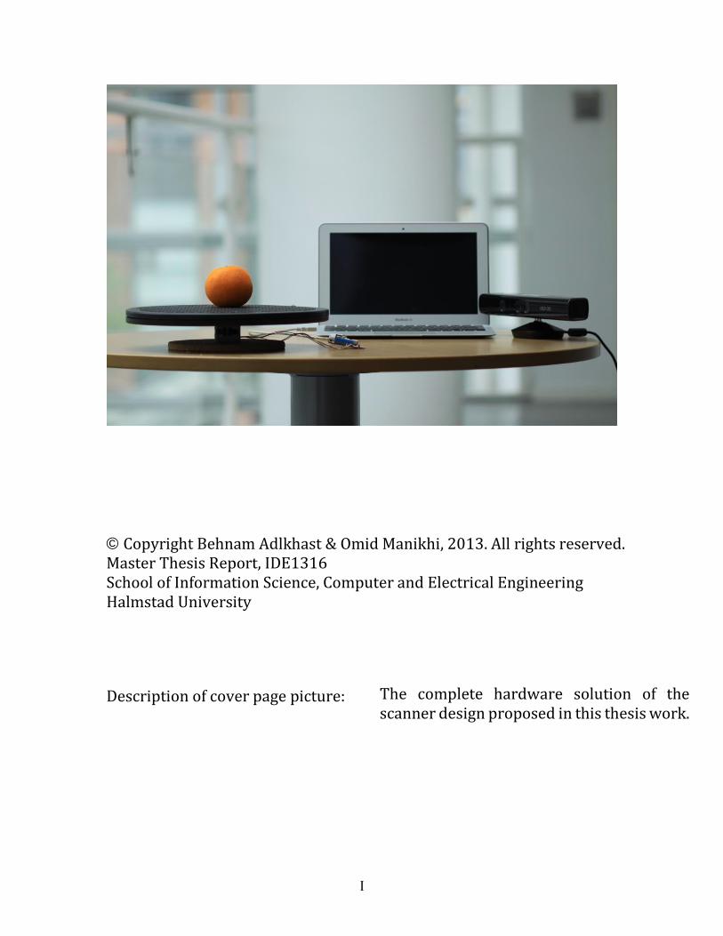
Description of cover page picture:

The complete hardware solution of the scanner design proposed in this thesis work.

II

Preface

We would like to express our deepest gratitude towards Dr. Björn Åstrand and Prof. Antanas Verikas for all their technical and moral support during the course of this project.

Behnam Adlkhast & Omid Manikhi

Halmstad University, October 2013

III

IV

Abstract

In this thesis report, an approach to use Microsoft Kinect to scan an object and provide a 3D model for further processing has been proposed. The additional required hardware to rotate the object and fully expose it to the sensor, the drivers and SDKs used and the implemented software are discussed. It is explained how the acquired data is stored and an efficient storage and mapping method requiring no special hardware and memory is introduced. The solution proposed circumvents the Point Cloud registration task based on the fact that the transformation from one frame to the next is known with extremely high precision. Next, a method to merge the acquired 3D data from all over the object into a single noise-free model is proposed using Spherical Transformation and a few experiments and their results are demonstrated and discussed.

V

VI

Contents

Introduction ..................................................................... 1

1.1 Background ........................................................................................... 1

1.2 Goals ........................................................................................................ 2

1.3 Problem Specification ....................................................................... 2 1.3.1 Data Acquisition .............................................................................................................................. 2 1.3.2 Storage ................................................................................................................................................ 2 1.3.3 Registration ...................................................................................................................................... 3 1.3.4 Post Processing ............................................................................................................................... 3 1.3.5 Results ................................................................................................................................................. 3

1.4 Social Aspects, Sustainability, Ethics ............................................ 3

State of the Art ................................................................ 5

Theory ............................................................................. 11

Required Hardware ....................................................... 15

4.1 Sensor .................................................................................................. 15

4.2 Rotating plate .................................................................................... 16

4.3 Stepper motor ................................................................................... 16

4.4 Stepper motor driver (EiBot) ...................................................... 17

Required Software ......................................................... 19

5.1 Drivers and Programming Tools ................................................ 19 5.1.1 Kinect for Windows SDK .......................................................................................................... 19 5.1.2 PCL (Point Cloud Library) ........................................................................................................ 19

5.2 3DScanner v1.0 64-Bit .................................................................... 19

Hardware Setup, Calibration and Application Settings

21

6.1 Microsoft Kinect ............................................................................... 21

6.2 Rotating plate .................................................................................... 21

6.3 Sensor’s pitch angle ......................................................................... 22

6.4 Calibration .......................................................................................... 23 6.4.1 Closest Point determination ................................................................................................... 23 6.4.2 Region of Interest (ROI) ............................................................................................................ 24 6.4.3 Base Center .................................................................................................................................... 26

Data Acquisition ............................................................ 29

7.1 Depth image preparations ............................................................ 30 7.1.1 Read a new depth image ........................................................................................................... 30 7.1.2 For each pixel in the depth image ......................................................................................... 30

7.2 Scanning .............................................................................................. 34 7.2.1 Rotation ........................................................................................................................................... 34 7.2.2 Transformation ............................................................................................................................ 34

VII

7.2.3 Registration ................................................................................................................................... 36

Storage ............................................................................ 39

8.1 Spherical model arrays .................................................................. 40 8.1.1 N-Model array ............................................................................................................................... 43 8.1.2 M-Model array .............................................................................................................................. 43 8.1.3 Mapping Spherical coordinates to array index ............................................................... 43 8.1.4 Mapping array index to Spherical coordinates ............................................................... 44

Merging ........................................................................... 47

9.1 The Merge process ........................................................................... 49 9.1.1 Using Spherical transformation to merge Point Clouds .............................................. 50 9.1.2 Outlier rejection ........................................................................................................................... 52 9.1.3 The Algorithm ............................................................................................................................... 54 9.1.4 Additional passes......................................................................................................................... 55

Experiments, Results & Discussion .............................. 57

10.1 Experiment 1 – Single objects ...................................................... 57 10.1.1 The role of each variable parameter .............................................................................. 57 10.1.2 The Pole-effect ......................................................................................................................... 64 10.1.3 A more complex object – The camera ............................................................................ 66

10.2 Experiment 2 – Multiple objects ................................................. 68

10.3 Evaluation against ground truth ................................................. 70

10.4 Evaluation of a competitor’s solution against ground truth 75

10.5 Discussion ........................................................................................... 78

Conclusion ...................................................................... 83

Bibliography ................................................................... 85

Appendix ......................................................................... 89

A.1 EiBot control commands ............................................................... 89

VIII

Figures

FIGURE 1.1 – 3D OBJECT SCANNING PROCESS STEPS ....................................................................................................2 FIGURE 2.1 - CURVED LINES ON THE 3D OBJECT RESULTING FROM THE PROJECTION STRUCTURED LIGHT [PICTURE ADOPTED FROM

[9]] ..........................................................................................................................................................5 FIGURE 2.2 - SYSTEMATIC LAYOUT OF OMNI VISER [PICTURE ADOPTED FROM [11]] .........................................................6 FIGURE 2.3 - HUMAN BODY SCANNING [PICTURE ADOPTED FROM [12]] ........................................................................7 FIGURE 2.4 - T-SHAPE BODY SCANNING [PICTURE ADOPTED FORM [13]] ........................................................................7 FIGURE 2.5 - PROCESS OF SCANNING A PERSON [PICTURE ADOPTED FROM [14]] ..............................................................8 FIGURE 3.1 - PRELIMINARY SCAN RESULTS OF A SIMPLE CUBOIDAL OBJECT. ....................................................................12 FIGURE 3.2 - HORIZONTAL SLICE OF THE TOP OF THE CUBOIDAL OBJECT. ........................................................................13 FIGURE 3.3 - THE HORIZONTAL SLICE OF THE TOP OF THE OBJECT, AVERAGED ALONG THE RADIUSES OF EACH SLICE. ...............13 FIGURE 4.1 - THE ROTATING PLATE, STEPPER MOTOR AND EIBOT.................................................................................15 FIGURE 4.2 - MICROSOFT KINECT ..........................................................................................................................16 FIGURE 4.3 - THE ROTATING PLATE ........................................................................................................................16 FIGURE 4.4 - EIBOT USB STEPPER MOTOR DRIVER. ..................................................................................................17 FIGURE 5.1 - 3DSCANNER V1.0 64-BIT. ................................................................................................................20 FIGURE 6.1 - POSITIONING THE KINECT...................................................................................................................21 FIGURE 6.2 - SENSOR'S PITCH ANGLE WITH RESPECT TO THE ROTATING PLATE ................................................................22 FIGURE 6.3 - SET ANGLE ......................................................................................................................................22 FIGURE 6.4 - CALIBRATE BASE ..............................................................................................................................23 FIGURE 6.5 - ERROR IN THE AUTOMATIC CLOSEST POINT DETERMINATION .....................................................................24 FIGURE 6.6 - ROI BOX, DIMENSIONS, PARAMETER CORRESPONDENCE...........................................................................25 FIGURE 6.7 - ROI BOUNDARIES .............................................................................................................................25 FIGURE 6.8 - ROI APPLIED ...................................................................................................................................26 FIGURE 6.9 - TEST OBJECT USED FOR CALIBRATION ....................................................................................................26 FIGURE 6.10 - (A) BEFORE CALIBRATION (B) AFTER CALIBRATION.................................................................................27 FIGURE 6.11 - CLOSEST POINT BEFORE AND AFTER CALIBRATION SHOWN IN FIGURE 6.10. ...............................................28 FIGURE 7.1 - DATA ACQUISITION PROCESS...............................................................................................................29 FIGURE 7.2 - INITIAL CAPTURED FRAME DIRECTLY AFTER CONVERSION TO GLOBAL METRIC COORDINATES .............................31 FIGURE 7.3 - THE RESULTING FRAME AFTER SENSOR ANGLE COMPENSATION. .................................................................32 FIGURE 7.4 - BOUNDING BOX IMAGINED AROUND OUR ROTATING PLATE AND OBJECT. .....................................................33 FIGURE 7.5 - FINAL POINT CLOUD AFTER CONVERSION, ROTATION AND FILTERING ..........................................................33 FIGURE 7.6 - SCANNING PROCESS. .........................................................................................................................34 FIGURE 7.7 - SPHERICAL COORDINATES REPRESENTATION ...........................................................................................37 FIGURE 7.8 - RENAME OF EACH AXIS. .....................................................................................................................38 FIGURE 7.9 - ROTATED AROUND THE AXIS OF ROTATION AND TRANSFORMED TO THE BASE CENTER. ....................................38 FIGURE 8.1 - SPHERICAL MODEL ARRAY ILLUSTRATION. ..............................................................................................41 FIGURE 8.2 - A SINGLE SPHERICAL ARRAY CELL WITH THE PROPOSED DIVISIONS COUNT. ....................................................42 FIGURE 9.1 - OVERLAY OF THE CAPTURED POINT CLOUDS AS A PREVIEW OF THE SCAN RESULTS. ........................................47 FIGURE 9.2 - THE SCANNED OBJECT’S TOP VIEW SHOWING THE NOISE AROUND ITS BORDERS. ............................................48 FIGURE 9.3 - A HORIZONTAL SECTION OF THE SCANNED OBJECT PLOTTED IN MATLAB.......................................................48 FIGURE 9.4 - DEMONSTRATION OF HOW WEIGHTED AVERAGE CAN DEFINE THE OBJECT'S BORDERS. ....................................49 FIGURE 9.5 - 2D POLAR NEIGHBORHOOD AND ITS CENTER OF GRAVITY .........................................................................50 FIGURE 9.6 - THE NEIGHBORHOOD REGION CONSIDERED AROUND EVERY VERTEX. ...........................................................52 FIGURE 9.7 - NEIGHBORHOOD PARAMETERS SETTINGS...............................................................................................53 FIGURE 9.8 - OUTLIER REJECTION SETTINGS. ............................................................................................................53 FIGURE 9.9 - MERGE PROCESS. .............................................................................................................................54 FIGURE 10.1 - CUBOIDAL TEST OBJECT. ..................................................................................................................57 FIGURE 10.2 - 3DSCANNER'S MAIN APPLICATION WINDOW. .......................................................................................58 FIGURE 10.3 - SETTINGS USED IN EXPERIMENT 1.1. ..................................................................................................58 FIGURE 10.4 - PRELIMINARY RESULTS OF EXPERIMENT 1.1. ........................................................................................59 FIGURE 10.5 - EXPERIMENT 1.1, PHASE 1 RESULTS. .................................................................................................60 FIGURE 10.6 - EXPERIMENT 1.1, PHASE 2 RESULTS WITH RHO RADIUS = 10 .................................................................60

IX

FIGURE 10.7 - EXPERIMENT 1.1, PHASE 2 RESULTS WITH RHO RADIUS = 15 .................................................................61 FIGURE 10.8 - EXPERIMENT 1.1, PHASE 2 RESULTS WITH RHO RADIUS = 35 .................................................................61 FIGURE 10.9 - POSSIBLE SIDE EFFECT OF RHO RADIUS INCREASE. A) RHO RADIUS = 5 B) RHO RADIUS

= 15 .......................................................................................................................................................62 FIGURE 10.10 - EXPERIMENT 1.1, PHASE 3 RESULTS WITH THETA AND PHI RADIUS = 2 ...................................................62 FIGURE 10.11 - EXPERIMENT 1.1, PHASE 3 RESULTS WITH THETA AND PHI RADIUS = 3 ...................................................63 FIGURE 10.12 - EXPERIMENT 1.1, PHASE 3 RESULTS WITH RHO RADIUS = 35 AND THETA AND PHI RADIUS = 4 ...................63 FIGURE 10.13 - EXPERIMENT 1.1, PHASE 4 RESULTS WITH OUTLIER REJECTION THRESHOLD = 20 .....................................64 FIGURE 10.14 - THE POLE-EFFECT HIGHLIGHTED USING THE YELLOW RECTANGLES. ..........................................................65 FIGURE 10.15 - SIZE OF NEIGHBORHOODS AND THEIR RELATIVE POSITION WITH RESPECT TO THE POLES. ..............................65 FIGURE 10.16 - THE CAMERA OBJECT. ....................................................................................................................66 FIGURE 10.17 - PRELIMINARY RESULTS OF EXPERIMENT 1.2 .......................................................................................66 FIGURE 10.18 - EXPERIMENT 1.2 RESULTS. .............................................................................................................67 FIGURE 10.19 - EXPERIMENT 1.2, PASS 2 RESULTS...................................................................................................68 FIGURE 10.20 - MULTIPLE OBJECTS. ......................................................................................................................68 FIGURE 10.21 - PRELIMINARY RESULTS OF EXPERIMENT 2 ..........................................................................................69 FIGURE 10.22 - EXPERIMENT 2, MERGE RESULTS .....................................................................................................69 FIGURE 10.23 - OBJECT USED TO FOR EVALUATION AGAINST GROUND TRUTH ................................................................70 FIGURE 10.24 - THE SCAN TO COMPARE AGAINST GROUND TRUTH ...............................................................................71 FIGURE 10.25 - GROUND TRUTH MODEL CREATED IN BLENDER ...................................................................................72 FIGURE 10.26 - GROUND TRUTH OBJECT AND ITS SCAN IMPORTED TO CLOUDCOMPARE ..................................................73 FIGURE 10.27 - GROUND TRUTH OBJECT AND ITS SCAN AFTER ICP REGISTRATION ...........................................................73 FIGURE 10.28 - SIGNED DISTANCE COLORED POINT CLOUD ........................................................................................74 FIGURE 10.29 - HISTOGRAM OF THE DISTANCE AGAINST GROUND TRUTH REFERENCE OBJECT ............................................75 FIGURE 10.30 - RESULT OF THE SCAN USING KINECTFUSION .......................................................................................76 FIGURE 10.31 - RESULT OF SCAN USING KINECTFUSION ALIGNED AGAINST GROUND TRUTH MODEL USING ICP .....................77 FIGURE 10.32 - SIGNED DISTANCE COLORED POINT CLOUD OF KINECTFUSION SCAN AGAINST GROUND TRUTH .....................77 FIGURE 10.33 - HISTOGRAM OF THE DISTANCE OF THE KINECTFUSION SCAN AGAINST GROUND TRUTH ...............................78 FIGURE 10.34 - SCANNING MULTIPLE OBJECTS USING KINECTFUSION. ..........................................................................80 FIGURE 10.35 - SCANNING A DETAILED OBJECT USING KINECTFUSION. .........................................................................80 FIGURE 10.36 - COMPARISON OF SCAN RESULTS AGAINST GROUND TRUTH BETWEEN TWO IMPLEMENTATIONS .....................81 FIGURE 11.1 - THE ENTIRE PROCESS .......................................................................................................................84

Tables

TABLE 1 - SPHERICAL MODEL ARRAY CELL SIZE. .........................................................................................................42 TABLE 2 - EXPERIMENT 1.1, PHASE 1 PARAMETERS. ..................................................................................................59 TABLE 3 - EXPERIMENT 1.2 PARAMETERS. ...............................................................................................................67 TABLE 4 - EXPERIMENT 1.2, PASS 2 PARAMETERS. ....................................................................................................67 TABLE 5 - EXPERIMENT 2, MERGE PARAMETERS .......................................................................................................70 TABLE 6 – EVALUATION AGAINST GROUND TRUTH, MERGE PARAMETERS ......................................................................71 TABLE 7 – RESULTS OF THE EVALUATION AGAINST GROUND TRUTH ...............................................................................74 TABLE 8 – RESULTS OF THE EVALUATION OF KINECTFUSION SCAN AGAINST GROUND TRUTH ..............................................76

A 3D Object Scanner

1

Introduction

1.1 Background

Since the introduction of Microsoft Kinect as a cheap consumer-level 3D sensor, the game plan has more or less changed. The introduction of a sensor that can provide depth data with a decent accuracy and with a quite cheap price has provided many enthusiasts with the tools required to realize their ideas and introduce new implementations and approaches to old problems.

The way Microsoft Kinect works, it projects a structured infrared laser dot pattern and using a CMOS sensor and an IR-Pass filter a depth map is generated by analyzing the relative distance of the dots on the objects. The projected dots become ellipse the direction of which depends on depth, and this change is due to the astigmatic lens of Kinect. If one looks closer and from another angle to the dots or ellipses, the closer ones are shifted more to the side than the farther ones. Kinect can analyze the shift of the dot pattern by projecting from one angle and observing from another and use that to build a depth map. [1], [2]

Scanning real world objects in order to build 3D models that can be stored and manipulated by computer programs has always been an active field of research. There have been different approaches and different techniques using different sensors and they all have their cons and pros.

Our focus in this thesis report is to suggest one approach to application of the Microsoft Kinect in building a 3D object scanner using basic components and without the need for high-end computers and fancy video adapters. We test how a 3D reconstruction system can work when accurate transformations of the camera are known. By sampling equidistantly around the object, we thus are not in need of doing the point cloud registration task. While some methods show very promising results using point cloud registration e.g. KinectFusion [3] there is an elementary problem that can never be fully solved by such algorithms. Error in estimated transformation from one viewpoint to the next contains error, which will propagate through the process. This incurs an error in the final estimate. To compensate for this, approaches based on Particle [4] and Kalman filters [5] are usually adopted. This minimizes the effects, but does not remove them altogether. We investigate in this thesis work a setting where the transformation from one frame to the next is known with extremely high precision and test if this setting provides more reliable results than the more sophisticated methods based on registration. Furthermore, because we know the transformations beforehand (circular movements around the object) we experiment with using a coordinate frame especially suited.

A 3D Object Scanner

2

In short, the way it works is that the object put on a rotating plate would be rotated in specific steps using a stepper motor. This situation can be related to that of a human holding an object in his hands and trying to assess the shape of the object by moving it around in his hands to get a glimpse of its various angles. While rotating the object, the Microsoft Kinect being fixed on a tripod is looking down on it and sending the depth data to the application, which will store and merge them later to generate a full 3D model of the object.

1.2 Goals

The goal of this work is to propose an approach using Microsoft Kinect to scan an object and provide a 3D model of it for further processing and application in a computer program. The model generated should be as close as possible to the original object and preserve a decent degree of detail. The scanner is not intended to scan very small and detailed objects as the accuracy provided by the sensor prevents such applications.

1.3 Problem Specification

Figure 1.1 – 3D object scanning process steps

The problem of scanning a 3D object from start to finish is a multi-step complex process, which can be broken down into the main sub-problems shown in Figure 1.1.

Each stage is thoroughly attended to, but a brief description of each sub-problem is given below.

1.3.1 Data Acquisition

The data acquisition stage includes capturing depth data from all the around an object and performing the necessary operations to prepare the captured data for storage.

1.3.2 Storage

This stage determines how the data acquired can be stored, retrieved and manipulated by the proceeding stages.

Data Aquisition

Storage RegistrationPost

ProcessingResults

A 3D Object Scanner

3

1.3.3 Registration

The registration stage intends to align the overlapping data acquired and stored on top of each other to form the final object shape.

1.3.4 Post Processing

Since the depth data collected from the sensor contains a considerable amount of noise, which comes from the large uncertainty around voxels, they will not be of much use before applying some techniques to reduce that noise and remove the fluctuations around surfaces.

1.3.5 Results

This stage consists of the providing the visual and binary form of the generated and processed model for further processing and use to the user.

1.4 Social Aspects, Sustainability, Ethics

In a world where more and more processes everyday are transforming into computer simulation and modeling problems, the need for 3D scanners is quite obvious. A 3D scanner can save a huge amount of time and money by providing a starting point for a design for example in the fashion business or industrial design or many other fields.

A fashion designer for instance, can scan his models’ bodies and design clothes and accessories that fit them perfectly without cutting a single piece of cloth! This can of course save a huge amount of fabrics used in design trial and errors, prototypes, demos, etc. which in turn contribute to much less pollution of the air by fabric factories and much less animal fatalities to produce yarn.

In fashion stores, a 3D scanner can be used to scan a person’s body and show them how they would look like in different clothes without actually wearing them. Again, the amount of time people save when shopping and the amount of clothes saved from accidental damages while being tried on by many different people as well as the hygienic aspects of it are easy to see benefits.

The added dimension to the ordinary images taken using cameras makes detection and identification of 3D objects a lot easier. A 3D scanner is the first step in feeding smart applications their training material to be able to serve as smart appliances, cars, planes, etc.

Finally yet importantly, making 3D scanning cheaper and available to a wider spectrum of public unleashes new waves of creativity and saves people time and

A 3D Object Scanner

4

money and of course the environment. We are hoping that we have made a yet small contribution in that direction.

A 3D Object Scanner

5

State of the Art

There have been many different solutions proposed over the years using different sensors and different techniques. Laser scanners, structured light scanners and stereo vision scanners are a few of them. A few of the solutions and methods relevant to our work are briefly discussed in this chapter.

For example [6] uses a cheap 2D Laser range scanner to sweep the scene and then with a little help from the user by choosing a few similar points between the two Point Clouds uses them as the initial guess to help the ICP (Iterative Closest Point) algorithm introduced in [7] to converge. This scanner however, is meant to scan environments rather than single objects.

As another example, [8] uses a colorful structured pattern of light and a catadioptric camera in making a 3D endoscope unit capable of providing the doctor with a 3D view of its field of operation rather than just a 2D image. As most other structured light scanners, this one uses triangulation to reconstruct the 3D surfaces too.

Next, [9] presents a framework to compress profitable PointClouds attained by 3D scanning using structured lights. In order to achieve this, they designed a pattern, which includes both vertical and horizontal lines projected on the object to be scanned. 3D points are projected on the lines that look like curves on the 3D object as shown in Figure 2.1. Based on these sequential curved points the points on the curves can be decoded. Using the decoded points the next best possible point on the curve is predicted added to the set of corrective vectors while each point keeps their previous decoded point. Scalar quantization has been used to map this set of vectors.

Figure 2.1 - Curved lines on the 3D object resulting from the projection structured light [Picture adopted from [9]]

A 3D Object Scanner

6

Moreover [10] has proposed another 3D laser scanner using two CCD cameras and servo motion system again applying the principle of optical triangulation.

Figure 2.2 - Systematic Layout of Omni Viser [Picture adopted from [11]]

Likewise, [11] presents a scanner by linking a rotating laser with Omni directional (360°) view. Real time 3D scanning, the ability to be installed on other devices and outdoor real time 3D scanning are achievements of this solution. The solution uses a stepper motor and a stepper motor controller, an Omni Camera, Hokuyo UTM-30LX Sensor with a 270° scanning range and wireless communication capabilities. The solution gathers 3D data as 3D PointClouds and represents them in a Cartesian coordinate system by using forward kinematics. The depth image is generated by compounding all range of 3D PointCloud data into a 2D matrix. Finally, to calculate optimal results, non-linear least square estimation is used.

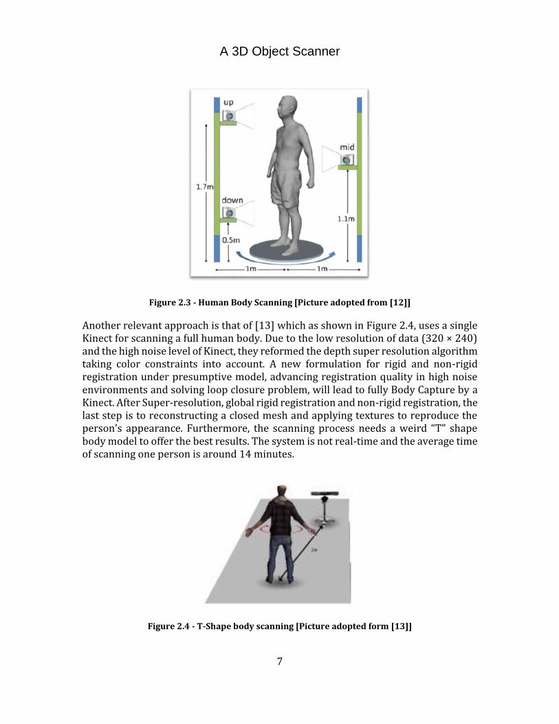
Another interesting work is the one presented in [12] which uses three Kinects to scan a full human body in 3D. This has been achieved thanks to Non-rigid alignment, loop closure constraint and complex occlusions. Non-rigid alignment is used as the registration technique for the scanned data. This system has been incorporated as a virtual 3D try-on of clothes on a human. This solution is shown in Figure 2.3.

A 3D Object Scanner

7

Figure 2.3 - Human Body Scanning [Picture adopted from [12]]

Another relevant approach is that of [13] which as shown in Figure 2.4, uses a single Kinect for scanning a full human body. Due to the low resolution of data (320 × 240) and the high noise level of Kinect, they reformed the depth super resolution algorithm taking color constraints into account. A new formulation for rigid and non-rigid registration under presumptive model, advancing registration quality in high noise environments and solving loop closure problem, will lead to fully Body Capture by a Kinect. After Super-resolution, global rigid registration and non-rigid registration, the last step is to reconstructing a closed mesh and applying textures to reproduce the person’s appearance. Furthermore, the scanning process needs a weird “T” shape body model to offer the best results. The system is not real-time and the average time of scanning one person is around 14 minutes.

Figure 2.4 - T-Shape body scanning [Picture adopted form [13]]

A 3D Object Scanner

8

The solution proposed in [14], tries to scan and print a 3D model of several people with Kinect by tracking the camera pose and generating the dense 3D model. Furthermore, an algorithm has been presented to register the depth image on the color image. Each voxel needs a color function, a weight function and a signed distance function. They have also presented a method to automatically fill the holes. In order to display the model generated by the registration of the color and depth values of each cell of the voxel grid, the data is copied every 2 seconds from the GPU to the memory and manipulated as a separate thread in the CPU by a Marching Cubes Algorithm [15] . In order to make a scanned 3D object printable they added the SDF (Signed Distance Function) layers from all sides, which ensure that triangle mesh is closed, watertight and printable. The process is shown in Figure 2.5.

Figure 2.5 - Process of scanning a person [Picture adopted from [14]]

This approach is dependent on the GPU rather than the CPU which we tried to avoid.

Another approach by [16], tries to achieve acceptable 3D scanning results from noisy image and range data in a room environment. They try to separate the person from the background to make a 3D model of them. The algorithm proposed tries to extract accurate results from the poor resolution and accuracy of the sensor. As a person moves, it is impossible to make a rigid 3D alignment. To solve this issue, they used SCAPE model [17], which is the parametric 3D model that factors the non-rigid deformation induced by both shape and variation. Calibration, body modeling and fitting are the next steps. Intrinsic calibration, stereo calibration and depth calibration lead to the next level of scanning. They calculated the metric accuracy of body shape fitting using both image contours and image depths.

One other relevant approach to automatic registration of PointClouds is the one proposed by [18]. This technique uses the estimation of 3D rotations from two different Gaussian images to achieve Crude alignment. In order to do so, Fourier domain transformations, spherical and rotational harmonic transforms and finally ICP with only a few iterations have been used. These algorithms cause the PointClouds to overlap. In order to get around that, correlation-based formulation

A 3D Object Scanner

9

that can correlate image captures of the point cloud has been proposed. This can decrease overlapping but not completely eliminating it.

Perhaps the most interesting and relevant approach is that of the KinectFusion presented in [19] which introduces a solution that uses Microsoft Kinect as the capture device and allows real-time reconstruction of detailed 3D scenes by having the Kinect moved around. The solution uses ICP as the registration algorithm [7] to find the position of the sensor within the environment using the assumption that position changes between two consecutive frames are minor as well as TSDF (Truncated Signed Distance Function) first introduced in [20] to merge every newly captured frame into the model. This method is nearly flawless; however, it requires a powerful GPU to store the model and to allow parallel execution of sophisticated algorithms on the GPU and to constantly update the TSDF volume.

Our solution however requires no additional processing power than an ordinary computer and differs in the sense that it is not a real-time scanner but an offline one. Unfortunately it was impossible to access all the mentioned sensors and implementations to evaluate their results against ours but the KinectFusion being the most popular and active Kinect-based solution was used as a competitor to give a clear idea of how well our solution works against the competition.

A 3D Object Scanner

10

A 3D Object Scanner

11

Theory

As the intention of this work has been from the beginning, the sensor used to capture the depth data is the Microsoft Kinect. In this chapter, a solution to implement the 3D Scanner desired and formulated in chapter 1 has been proposed. The general theory behind the approach will be briefly discussed while they are discussed in depth in chapters 4 to 9.

In order to acquire the depth data from all the angles of an object, the object is rotated 360 degrees while the sensor is still and oriented towards the object. The rotation is done using a circular plate coupled with a stepper motor. The stepper motor was chosen as the rotation device since it can be accurately rotated in specific angles, which can later be used to register the captured data. Initially, the sensor was roughly on the same plane as the object to be scanned. However this posed a problem in the sense that sometimes the top face of an object remained unexposed to the sensor. One solution to this problem as we have chosen it is to slightly tilt the sensor downwards and place the sensor in a higher plane than the object to be scanned.

Since the area which embodies the object is a limited area and the rest is irrelevant for us, parts of every captured frame with irrelevant background objects can be discarded. This significantly improves the speed.

The acquired data is of course in the sensor’s frame of reference. They need to be transformed to a global frame of reference. This global frame has been considered centered on the rotating plate. During the course of a full scan cycle, 50 frames are captured from equally spaced rotation angles.

Although the acquired data are originally in Cartesian space, since our method revolves around the operations done in the Spherical space, they need to be converted and stored in such container. The storage needs to store all the captured depth information during the course of a full scan. In order to do so an approach was adapted based on Certainty Grids introduced by [21], [22]. Each cell of the container corresponds to a voxel in the global space and holds the certainty value of the existence of that voxel. Each time a voxel in the global space is observed, its certainty value is increased in the grid. This way we can store all the captured frames from all around the object after having transformed and rotated them around the center of the plate. This also concludes the registration stage.

The acquired and stored data are still far too noisy to be usable and thus the necessity of post processing and noise reduction becomes clear. Each voxel of the depth data captured from Kinect tends to fluctuate approximately perpendicular to the surface along the sensor’s line of sight. Using the Certainty Grid storage approach used, the best estimate would be to weighted average the fluctuations in order to find the points that are more likely on the surface of the object. The question that remains is

A 3D Object Scanner

12

regarding the axis along which the average must be calculated. Since the data is acquired having the sensor capture the depth information in a circular manner around the object and considering the simple case that the object is centered on the rotating plate, the first solution that comes to one’s mind is averaging the certainty values of each group of voxels along the radius of a horizontal slice of the cylinder embodying the object. Although this works with certain objects, in cases such as an object with a flat top, the average will destroy the shape of the object by averaging a plane and turning it into a polygon!

In order to further clarify this, if we take a simple cuboidal object and scan it, the preliminary results will look something like Figure 3.1.

Figure 3.1 - Preliminary scan results of a simple cuboidal object.

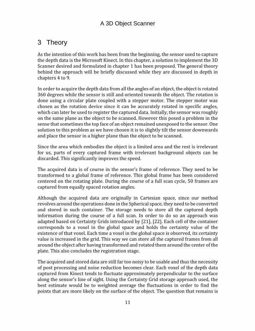
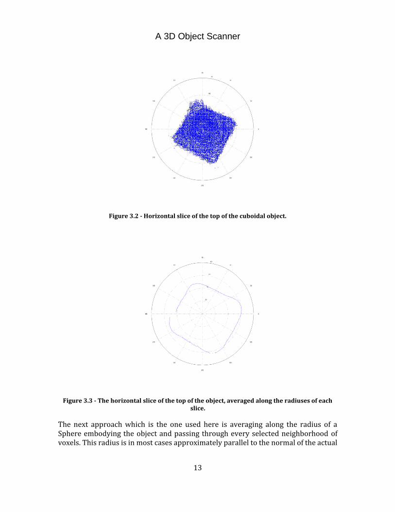
If we take a horizontal slice of the top of the object and draw it, it would look something like Figure 3.2. Now as a simple case, if we average the certainty values of equal slices all around the plate and along the radiuses of each slice, the result will be not a plane of voxels but a polygon! This would have worked just fine for the walls of the object but apparently not for the top face. The result has been shown in Figure 3.3.

A 3D Object Scanner

13

Figure 3.2 - Horizontal slice of the top of the cuboidal object.

Figure 3.3 - The horizontal slice of the top of the object, averaged along the radiuses of each slice.

The next approach which is the one used here is averaging along the radius of a Sphere embodying the object and passing through every selected neighborhood of voxels. This radius is in most cases approximately parallel to the normal of the actual

A 3D Object Scanner

14

surface and can provide a good direction of averaging. This justifies the need to store the data in a Spherical model, which can make grouping voxels in neighborhoods much easier.

The following chapters will go through the details of the methods used to put this theory to action.

A 3D Object Scanner

15

Required Hardware

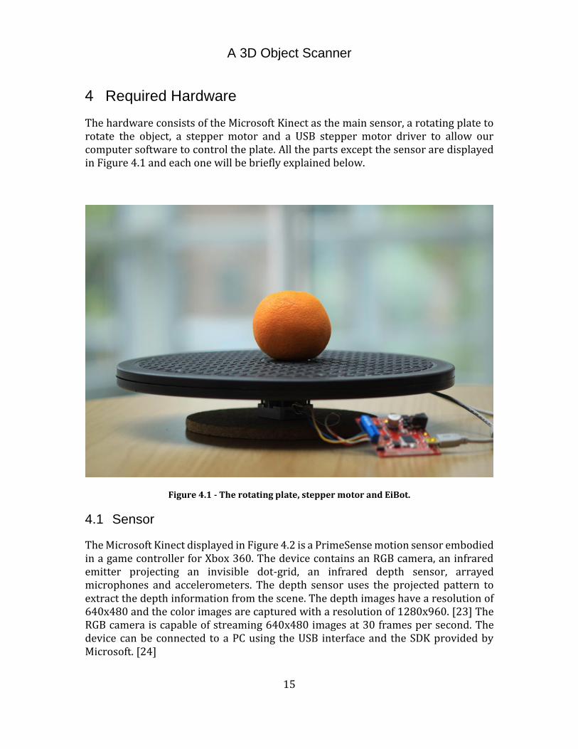
The hardware consists of the Microsoft Kinect as the main sensor, a rotating plate to rotate the object, a stepper motor and a USB stepper motor driver to allow our computer software to control the plate. All the parts except the sensor are displayed in Figure 4.1 and each one will be briefly explained below.

Figure 4.1 - The rotating plate, stepper motor and EiBot.

4.1 Sensor

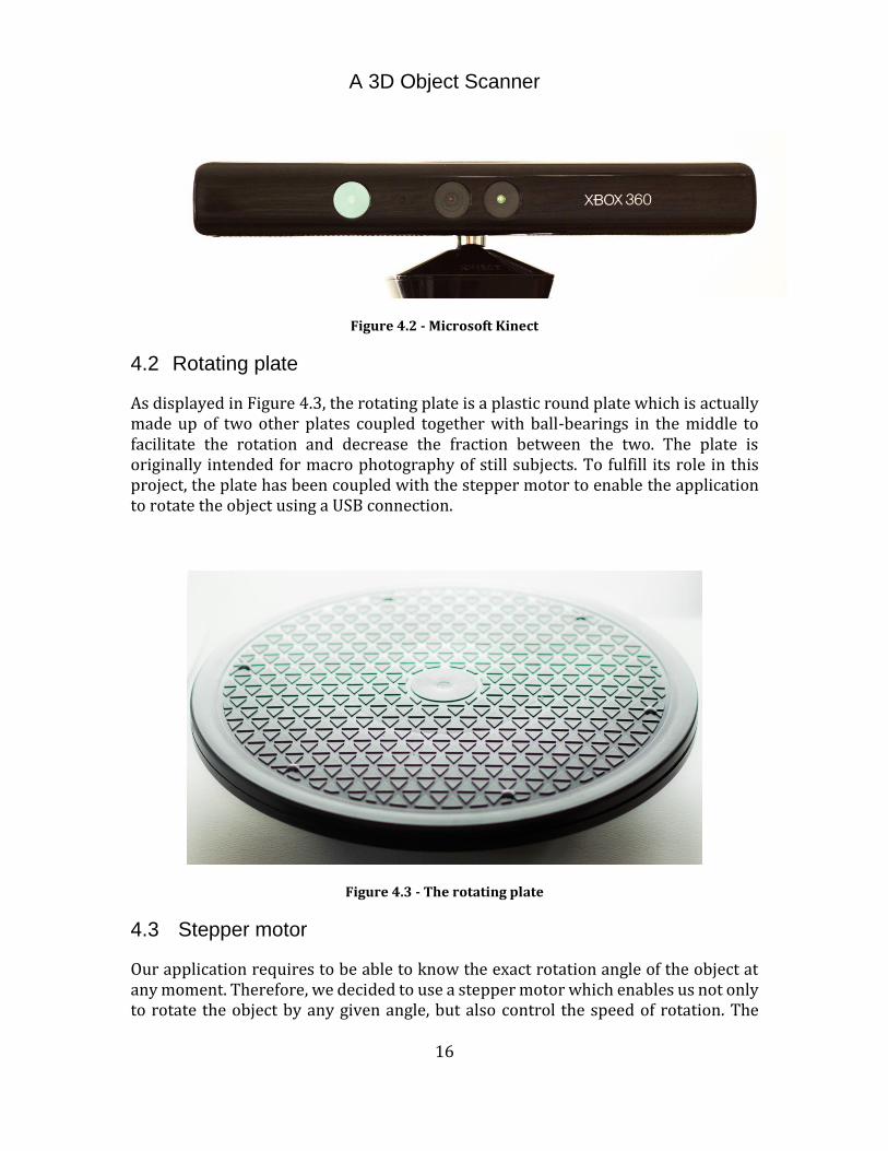
The Microsoft Kinect displayed in Figure 4.2 is a PrimeSense motion sensor embodied in a game controller for Xbox 360. The device contains an RGB camera, an infrared emitter projecting an invisible dot-grid, an infrared depth sensor, arrayed microphones and accelerometers. The depth sensor uses the projected pattern to extract the depth information from the scene. The depth images have a resolution of 640x480 and the color images are captured with a resolution of 1280x960. [23] The RGB camera is capable of streaming 640x480 images at 30 frames per second. The device can be connected to a PC using the USB interface and the SDK provided by Microsoft. [24]

A 3D Object Scanner

16

Figure 4.2 - Microsoft Kinect

4.2 Rotating plate

As displayed in Figure 4.3, the rotating plate is a plastic round plate which is actually made up of two other plates coupled together with ball-bearings in the middle to facilitate the rotation and decrease the fraction between the two. The plate is originally intended for macro photography of still subjects. To fulfill its role in this project, the plate has been coupled with the stepper motor to enable the application to rotate the object using a USB connection.

Figure 4.3 - The rotating plate

4.3 Stepper motor

Our application requires to be able to know the exact rotation angle of the object at any moment. Therefore, we decided to use a stepper motor which enables us not only to rotate the object by any given angle, but also control the speed of rotation. The

A 3D Object Scanner

17

stepper motor we used is a 4H4018S2935(122/H) from Landa Electronics, which is a Bipolar stepper motor with a rated voltage of 4.5 Volts, and each of its rotation steps are 1.8 degrees. [25]

Another possible alternative would be a gear-boxed DC Motor with an encoder, however given the fact that the Stepper Motor chosen allows rotation angles as small as 1/16th of the rotation step, it is far more accurate than an encoder-coupled DC Motor. This enables rotation steps of as small as 0.1125 degrees.

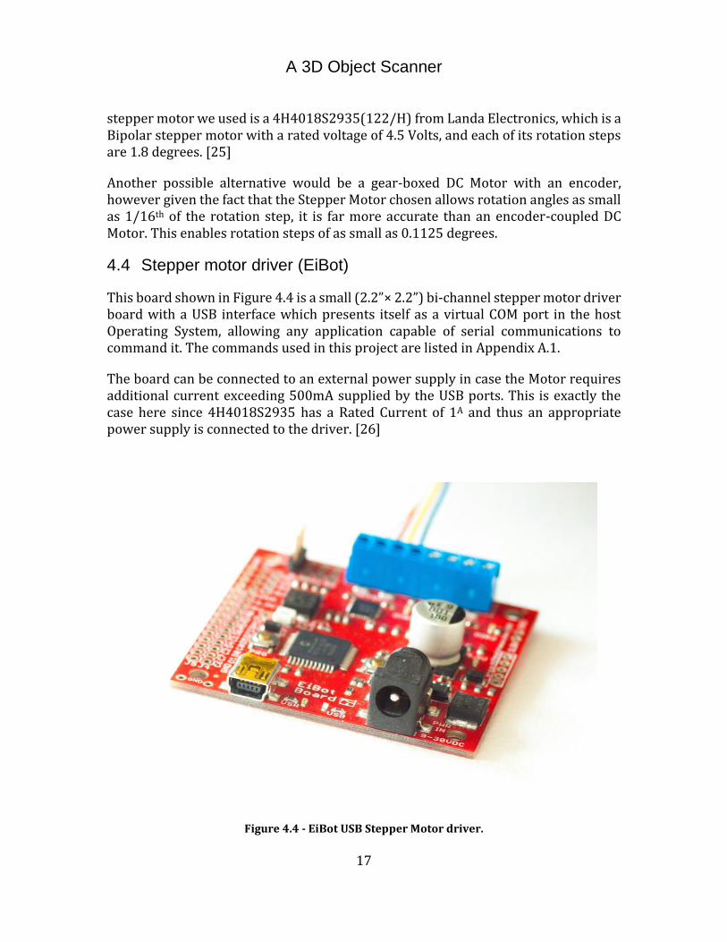
4.4 Stepper motor driver (EiBot)

This board shown in Figure 4.4 is a small (2.2”× 2.2”) bi-channel stepper motor driver board with a USB interface which presents itself as a virtual COM port in the host Operating System, allowing any application capable of serial communications to command it. The commands used in this project are listed in Appendix A.1.

The board can be connected to an external power supply in case the Motor requires additional current exceeding 500mA supplied by the USB ports. This is exactly the case here since 4H4018S2935 has a Rated Current of 1A and thus an appropriate power supply is connected to the driver. [26]

Figure 4.4 - EiBot USB Stepper Motor driver.

A 3D Object Scanner

18

A 3D Object Scanner

19

Required Software

This chapter goes through the required, harnessed and developed drivers, SDKs, libraries and applications to achieve the desired functionality.

5.1 Drivers and Programming Tools

The Drivers and Programming tools incorporated in the development of this application are briefly discussed below. These include the Microsoft Kinect SDK [27] Which is the interface between the application and the sensor as well as the PCL (Point Cloud Library) which is used to store and mainly visualize Point Clouds. A Point Cloud is a data structure capable of storing in general multidimensional and in particular 3D data representing X, Y and Z coordinates of every point. [28]

5.1.1 Kinect for Windows SDK

The Kinect for Windows SDK provides the programming tools and APIs required to read Audio, Color and Depth and Skeletal data from Microsoft Kinect as well as methods to process and convert them.

The SDK comes with Drivers for the sensor itself, documentation, samples, tutorials and a complete API reference.

Our application used Kinect for Windows SDK v1.6. [27]

5.1.2 PCL (Point Cloud Library)

The Point Cloud Library (or PCL) is an open source library intended to provide input/ output functionality and algorithms for processing and perception of Point Clouds. The library provides many state-of the-art algorithms such as feature estimation, model fitting and so on.

Our use of the PCL is mainly limited to visualizing Point Clouds as well as some of its fundamental Point Cloud processing and storage functionality. [29]

In our application, we are using PCL v1.6.0 compiled for Microsoft Visual Studio 2010 and Microsoft Windows x64.

5.2 3DScanner v1.0 64-Bit

The application developed for this project is named “3DScanner v1.0” and has been developed using Microsoft Visual C++ 2010 and compiled for 64-Bit versions of Windows. The name comes from the history that it was meant to be interfaced with two different sensors in the beginning so it was renamed from “KinectScanner” which

A 3D Object Scanner

20

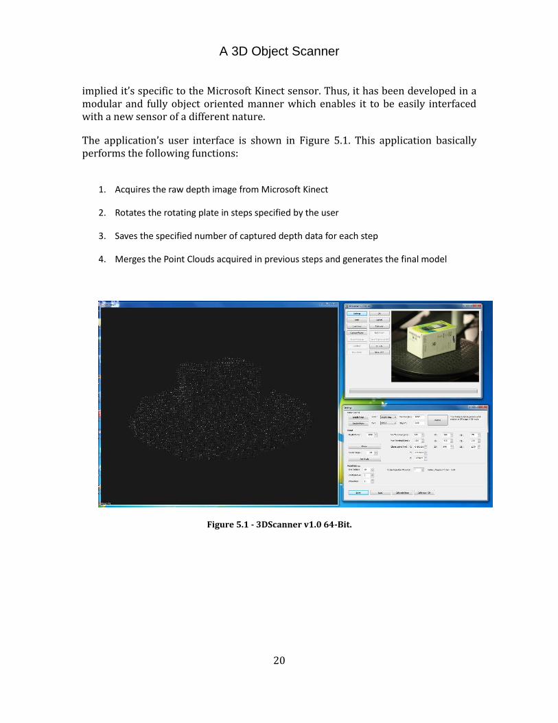
implied it’s specific to the Microsoft Kinect sensor. Thus, it has been developed in a modular and fully object oriented manner which enables it to be easily interfaced with a new sensor of a different nature.

The application’s user interface is shown in Figure 5.1. This application basically performs the following functions:

1. Acquires the raw depth image from Microsoft Kinect

2. Rotates the rotating plate in steps specified by the user

3. Saves the specified number of captured depth data for each step

4. Merges the Point Clouds acquired in previous steps and generates the final model

Figure 5.1 - 3DScanner v1.0 64-Bit.

A 3D Object Scanner

21

Hardware Setup, Calibration and Application Settings The following are necessary adjustments required to achieve the best results. The setup needs are kept minimal in order to simplify the manual initiatives necessary and to maximize the adaptability to different environments.

6.1 Microsoft Kinect

The correct way to position the sensor is shown in Figure 6.1. The Kinect is mounted on a tripod on a higher level than the top surface of the object about to be scanned. The level should be high enough that would allow the sensor to capture enough of the top surface as well as the front face of the object at the same time. The angle of the sensor will be set in the 3DScanner software later.

Figure 6.1 - Positioning the Kinect

6.2 Rotating plate

It is important that the rotating plate be placed in a manner that its front edge is the closest surface the sensor sees. This means that there should be no objects in the sensor’s field of view between the front edge of the plate and Microsoft Kinect.

A 3D Object Scanner

22

6.3 Sensor’s pitch angle

The sensor’s pitch angle as shown in Figure 6.2, is set through the application and is used to rotate the frame and align the rotating plate with the XZ plane as if the sensor was parallel to the horizon. The sensor’s pitch angle can be adjusted anywhere between -27 and +27 degrees with 0 being parallel to the horizon. Depending on how high the sensor is from the object, we adjust the angle using the Settings dialog as shown in Figure 6.3 so that the rotating plate is fully positioned inside the sensor’s field of view. Other than that, while setting the angle, it is important to find an angle in which the object has maximum visibility by the sensor and make sure all sides of the object can be seen by the sensor if the object is rotated. This is of course a product of the sensor placement and its height relative to the rotating plate. The value entered will be used to adjust the sensor’s elevation using its built-in motor and to compensate for the sensor’s pitch angle as described in 7.1.2.3. Kinect uses an accelerometer to adjust its angle with respect to gravity and has an accuracy of 1 degree. [30] The error can of course have a slight effect in the merged model but that is the best achievable with this method. One can of course manually measure the angle the sensor makes with the surface of the rotating plate to verify the value. Following the angle change, the user is able to see the preview and determine if the rotating plate and the object to scan are fully visible and roughly centered in the view.

Figure 6.2 - Sensor's Pitch angle with respect to the rotating plate

In our setup, the sensor is set at a -20 degrees angle with the horizon.

Figure 6.3 - Set angle

A 3D Object Scanner

23

Since at this stage we have not yet isolated the rotating plate from the rest of the scene, it is difficult to determine the pitch angle automatically.

6.4 Calibration

Calibration is an important initial step of the scanning process. The goal of this step is to set the global coordinates of the center of the rotating plate. This point together with the rotating plate’s radius is used in the transformations to correctly rotate and register the captured Point Clouds in the global model. The calibration process can be broken down into a few steps which we will go through each in this chapter.

6.4.1 Closest Point determination

The first step in the calibration process is to determine the coordinates of the closest point to the sensor. If as instructed in section 6.2, the front edge of the rotating plate is the closest point to the sensor, we can use this point together with the radius of the plate to find the center of the rotating plate. This is done simply by using the “Calibrate Base” function of our application as shown in Figure 6.4.

Figure 6.4 - Calibrate Base

A 3D Object Scanner

24

The resulting point is the point with minimum distance to the Sensor in 10 consecutive frames. This is our starting point for the rest of the calibration process.

The problem with this automatic calculated point is that due to excessive sensor noise, this point often differs in X and Z value with our ideal point. This can be clearly seen in Figure 6.5.

6.4.2 Region of Interest (ROI)

The ROI is an imaginary bounding box which surrounds the area we are interested in and any point that falls outside this box is neglected in the data acquisition phase.

These boundaries are automatically filled as part of the “Calibrate Base” functionality of the program. The way this is done is that after the Closest Point has been determined as explained in section 6.4.1, this point is used to form a 32𝑐𝑚 × 32𝑐𝑚 ×32𝑐𝑚 ROI corresponding to the dimensions of the rotating plate around it as shown in Figure 6.6.

Figure 6.5 - Error in the automatic Closest Point determination

A 3D Object Scanner

25

The parameters determining this region are shown in Figure 6.7. The relation between these values and the data acquired is displayed again in Figure 6.6.

These parameters can also be manually and visually adjusted in order to limit or expand the ROI to include only the object to be scanned and not the rotating plate in the scanning stage.

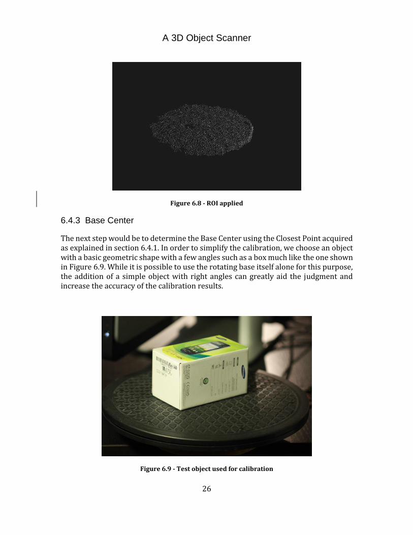
The result of the automatic determination of the ROI is shown in Figure 6.8.

Figure 6.6 - ROI box, dimensions, parameter correspondence.

Figure 6.7 - ROI boundaries

A 3D Object Scanner

26

Figure 6.8 - ROI applied

6.4.3 Base Center

The next step would be to determine the Base Center using the Closest Point acquired as explained in section 6.4.1. In order to simplify the calibration, we choose an object with a basic geometric shape with a few angles such as a box much like the one shown in Figure 6.9. While it is possible to use the rotating base itself alone for this purpose, the addition of a simple object with right angles can greatly aid the judgment and increase the accuracy of the calibration results.

Figure 6.9 - Test object used for calibration

A 3D Object Scanner

27

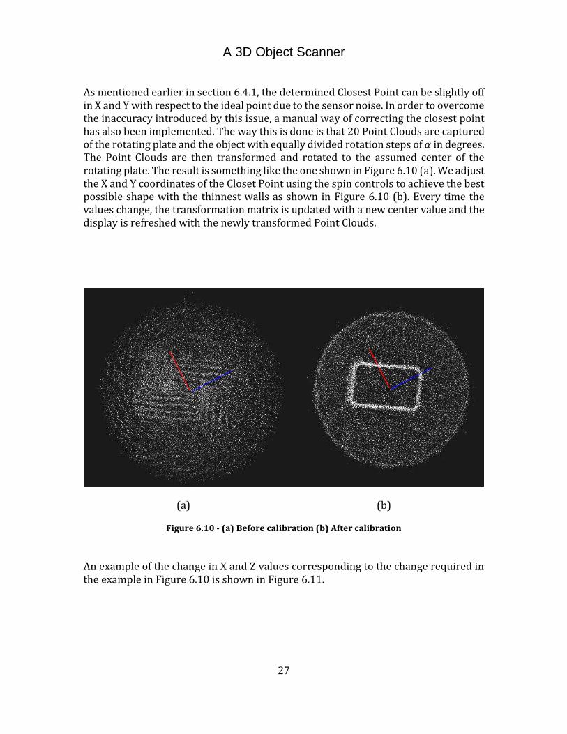
As mentioned earlier in section 6.4.1, the determined Closest Point can be slightly off in X and Y with respect to the ideal point due to the sensor noise. In order to overcome the inaccuracy introduced by this issue, a manual way of correcting the closest point has also been implemented. The way this is done is that 20 Point Clouds are captured of the rotating plate and the object with equally divided rotation steps of 𝛼 in degrees. The Point Clouds are then transformed and rotated to the assumed center of the rotating plate. The result is something like the one shown in Figure 6.10 (a). We adjust the X and Y coordinates of the Closet Point using the spin controls to achieve the best possible shape with the thinnest walls as shown in Figure 6.10 (b). Every time the values change, the transformation matrix is updated with a new center value and the display is refreshed with the newly transformed Point Clouds.

(a) (b)

Figure 6.10 - (a) Before calibration (b) After calibration

An example of the change in X and Z values corresponding to the change required in the example in Figure 6.10 is shown in Figure 6.11.

A 3D Object Scanner

28

Figure 6.11 - Closest Point before and after calibration shown in Figure 6.10.

A 3D Object Scanner

29

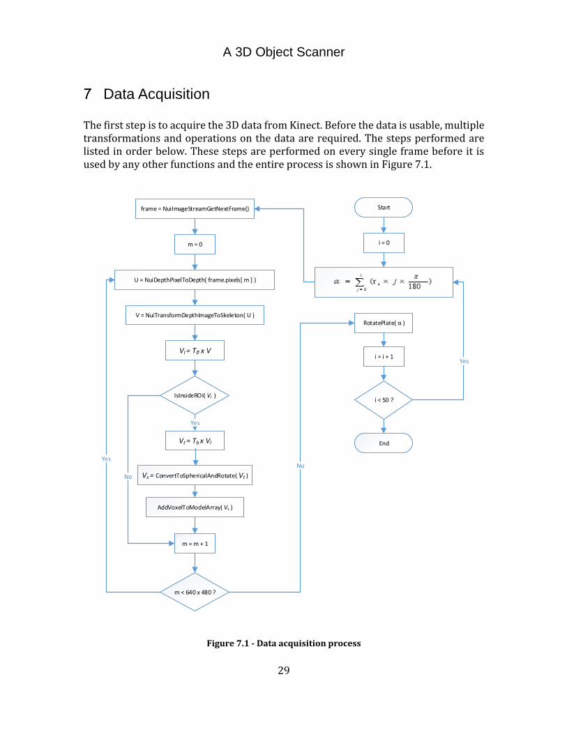
Data Acquisition The first step is to acquire the 3D data from Kinect. Before the data is usable, multiple transformations and operations on the data are required. The steps performed are listed in order below. These steps are performed on every single frame before it is used by any other functions and the entire process is shown in Figure 7.1.

frame = NuiImageStreamGetNextFrame()

m = 0

U = NuiDepthPixelToDepth( frame.pixels[ m ] )

V = NuiTransformDepthImageToSkeleton( U )

Vl = Tθ x V

IsInsideROI( Vl )

i = 0

Start

Vt = Tb x Vl

RotatePlate( α )

i < 50 ?

i = i + 1

Yes

AddVoxelToModelArray( Vs )

m = m + 1

m < 640 x 480 ?

Yes

No

No

Yes

End

Vs = ConvertToSphericalAndRotate( Vt )

Figure 7.1 - Data acquisition process

A 3D Object Scanner

30

7.1 Depth image preparations

7.1.1 Read a new depth image

The first step would be to read a raw depth image from the sensor. This is easily done using the Kinect for Windows SDK which from here on we refer to simply as the SDK. This is done using the following method: [31]

HRESULT NuiImageStreamGetNextFrame(

HANDLE hStream,

DWORD dwMillisecondsToWait,

const NUI_IMAGE_FRAME **ppcImageFrame

)

The ppcImageFrame here is of dimension 640 x 480 pixels.

7.1.2 For each pixel in the depth image

Next we go through the raw depth image of size (640 × 480) pixels, and perform the following steps on the extracted pixel.

Unpack the depth value

The depth value output by the SDK is a 16 bits value of which, bits 3-15 are the ones carrying the depth value and the rest hold the skeleton information. Thus, in order to extract the depth value, we need to shift the depth value 3 bits to the right. This is automatically done using the following method of the SDK: [31]

USHORT NuiDepthPixelToDepth(

USHORT packedPixel

)

The depth value acquired from this function, is in fact the distance of every point seen, from the sensor in millimeters. There’s still one more step before we can make good use of this triple.

Convert the image coordinates to global sensor coordinates

Next, we convert the image coordinates, which is basically the depth value of every image pixel, from the image frame to global metric coordinates. The origin of the new base is the sensor itself. This is done using the following method of the SDK: [31]

Vector4 NuiTransformDepthImageToSkeleton(

LONG lDepthX,

LONG lDepthY,

USHORT usDepthValue

A 3D Object Scanner

31

)

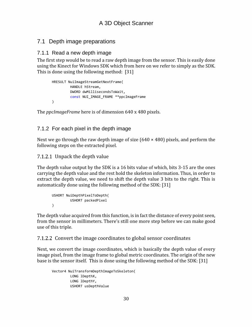
The output is a 3x1 vector containing the x, y and z values in meters. The resulting Point Cloud is shown in Figure 7.2. As can be seen, the sensor’s angle is shown in the picture.

Figure 7.2 - Initial captured frame directly after conversion to global metric coordinates

Compensating for the sensor’s pitch angle

Since we have setup the sensor slightly tilted to enable it to see the whole length of the object, we need to rotate the captured frame exactly the same amount to compensate the rotation. Thus, every point should be rotated ϴ degrees around the X axis, ϴ being the angle between the sensor and the horizon. This is done using a rotation matrix Tθ shown in Equation 5-1.

Tθ =[

1 0 0 00 cos𝛳 −sin𝛳 00 sin𝛳 cos𝛳 00 0 0 1

] (5-1)

A 3D Object Scanner

32

The final local point coordinates Vl is calculated by multiplying the original point coordinates V, by the rotation matrix as shown in Equation 5-2.

𝑉𝑙 = 𝑇𝜃 × 𝑉 (5-2) The resulting Point Cloud is shown in Figure 7.3.

Filtering points outside the ROI

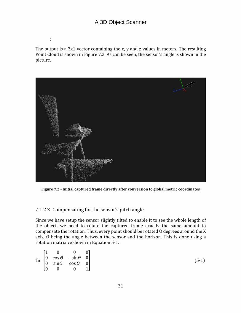
The last step would be to check whether the point lies within the boundaries of the ROI we set during the setup phase as mentioned in section 6.4.2. In order to do this, we imagine a box around our rotating plate and object and discard any points that are outside that box. Much like what is shown in Figure 7.4.

Figure 7.3 - The resulting frame after sensor angle compensation.

A 3D Object Scanner

33

Figure 7.4 - Bounding box imagined around our rotating plate and object.

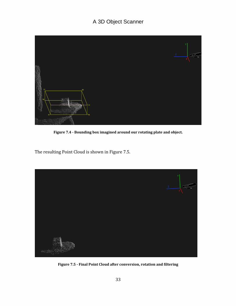
The resulting Point Cloud is shown in Figure 7.5.

Figure 7.5 - Final Point Cloud after conversion, rotation and filtering

A 3D Object Scanner

34

7.2 Scanning

Once the raw frame is prepared as described in chapter 7.1, we are ready to scan the object. Scanning is performed using the 3DScanner application and includes the operations shown in Figure 7.6.

Figure 7.6 - Scanning process.

The details of how the Point Clouds are stored are explained in chapter 8, but the rest will be explained below.

7.2.1 Rotation

The rotation is done by means of the commands we send to the EiBot stepper motor driver. The board’s Windows Driver installs a virtual Serial Port which allows any application to send commands using any standard terminal or in our case standard Window serial communication APIs. As a reference, the commands we have used are listed in appendix A.1.

7.2.2 Transformation

Every captured frame should go through another round of transformation to have it rotated and translated in order to be registered in its proper place inside the global model array.

As mentioned earlier, the scanner will rotate the plate 360° in rs steps calculated using Equation 5-3.

Rotates the object 360° in equal steps specified by the user

Captures a Point Cloud from each step

Transforms the captured Point Cloud and stores it in the global model array.

A 3D Object Scanner

35

𝑟𝑠 =360

𝑁𝑢𝑚𝑏𝑒𝑟 𝑜𝑓 𝑑𝑖𝑣𝑖𝑠𝑖𝑜𝑛𝑠 (5-3)

Number of divisions is the number of different angles we would like to capture a new Point Cloud from and is specified by the user based on the object’s complexity and size. Too few captured Point Clouds might leave some parts of a complex object unexposed and too many of them will unnecessarily increase the number of voxels and as a result the merging time. For our tests, we generally use 50 divisions, which prove to be a fair number providing a good balance between processing time and detail capture.

The rotation angle α of each step is calculated in radians using Equation 5-4.

𝛼 = ∑ (𝑟𝑠 × i ×𝜋

180)

𝑛

𝑖=1 (5-4)

The rotation plate center tb is calculated using the closest point calculated in chapter 6.4.1. If we consider the closest point tc as shown in Equation 5-5,

𝑡𝐶 = [

𝑋𝐶

𝑌𝐶

𝑍𝐶

] (5-5)

And the radius of the rotating plate was Rbase, the rotation plate center can be calculated according to Equation 5-6.

𝑡𝑏 = 𝑡𝐶 + [0

0

𝑅𝑏𝑎𝑠𝑒

] (5-6)

A 3D Object Scanner

36

Next, a transformation matrix is built to translate the Point Cloud to the rotation plate center. This is shown in Equation 5-7.

𝑇𝑏 = [

1 0 0 −𝑡𝑏𝑥

0 1 0 −𝑡𝑏𝑦

0 0 1 𝑡𝑏𝑧

0 0 0 1

] (5-7)

And thus, the translated coordinates Vt of the vertex is calculated using Equation 5-8 and will be in meters. The denoted Vl is the local coordinates of the vertex calculated using Equation 5-2.

𝑉𝑡 = 𝑇𝑏 × 𝑉𝑙 (5-8)

7.2.3 Registration

The next step would be to calculate the global coordinates of the vertex which is in fact the registration stage. This includes rotating the vertex around the rotation base center α degrees, which was calculated in Equation 5-4.

Since the storage and merging processes as will be thoroughly explained in Chapter 8 and Chapter 9 are all in the Spherical coordinates frame, switching the coordinates frame from here on would ease the registration and avoid further inaccuracy.

In order to convert a voxel’s coordinates from Cartesian to Spherical, Equation 5-9 can be used. Symbols 𝜌, 𝜃 and ∅ are denoted in Figure 7.7.

𝜌 = √𝑥2 + 𝑦2 + 𝑧2

𝜃 = cos−1 𝑧

𝜌 (5-9)

∅ = tan−1 𝑦

𝑥

Therefore, the inverse conversion from Spherical to Cartesian can be done using Equations 5-10.

𝑥 = 𝜌 sin∅ cos 𝜃 𝑦 = 𝜌 sin∅ sin 𝜃 (5-10)

A 3D Object Scanner

37

𝑧 = 𝜌 cos∅

𝜌 = √𝑥2 + 𝑦2 + 𝑧2

Figure 7.7 - Spherical coordinates representation

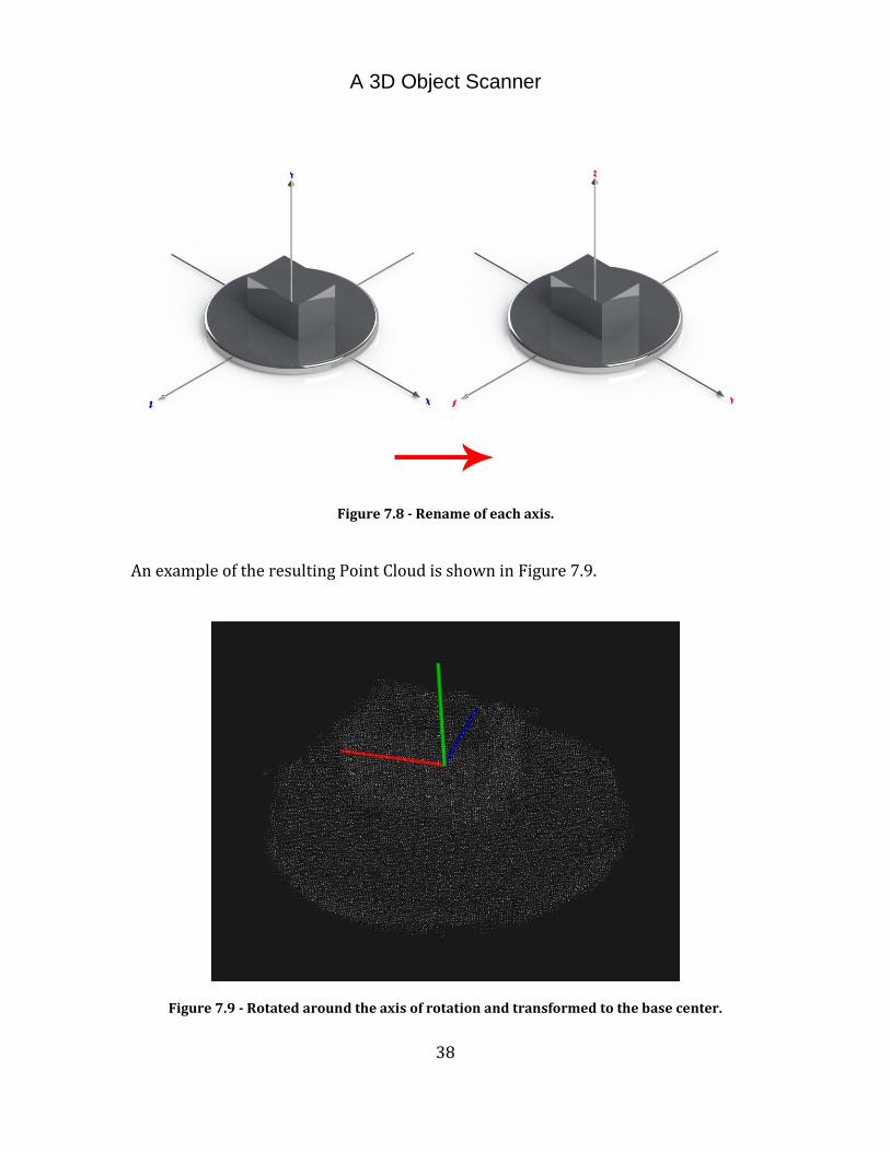
In order to simplify the registration, we would like to correlate the θ variable of the Spherical coordinates with the rotation angle α of the rotating plate. This means that in order to register every converted vertex, the registered global coordinates of that vertex has the same ϕ and ρ values but the θ is incremented by α radians. To do that, we rename each axis of Vt according to Equation 5-11 and as shown in Figure 7.8. 𝑥𝑉𝑡

→ 𝑧

𝑦𝑉𝑡→ 𝑥 (5-11)

𝑧𝑉𝑡→ 𝑦

And thus the global Spherical coordinates of each vertex Vs is calculated according to Equation 5-12.

𝑉𝑠 = [

𝜌𝜃

𝜑 + 𝛼] =

[ √𝑥2 + 𝑦2 + 𝑧2

cos−1 𝑧

√𝑥2+𝑦2+𝑧2

tan−1 𝑦

𝑥+ 𝛼 ]

(5-12)

A 3D Object Scanner

38

Figure 7.8 - Rename of each axis.

An example of the resulting Point Cloud is shown in Figure 7.9.

Figure 7.9 - Rotated around the axis of rotation and transformed to the base center.

A 3D Object Scanner

39

Storage After the scanning phase described in Chapter 7.2, the acquired data needs to be stored in a way that fulfills the following requirements. The storage we need should be:

Relatively lossless i.e. stores the data with an accuracy as closely as possible to what they

were captured with

Randomly accessible i.e. it is structured in a way that allows access to each Vertex given

its coordinates

Memory efficient i.e. would not require an unreasonable amount of memory

Fast i.e. the write access would allow real-time updates of every captured frame

The huge number of captured voxels need to be stored in a manner that fulfills all the requirements mentioned above as closely as possible. One option would be to use the Point Cloud data types in PCL. The PCL stores the voxels in an indexed manner which means, there’s no relation between the coordinates of a voxel and its index inside the Point Cloud. This makes it very difficult to iterate through a specific region of the voxels as in order to do so, one has to iterate through the whole Point Cloud once for every voxel. Apparently, this is far from efficient. On the other hand, using a three-dimensional array for every Point Cloud acquired from every single step of rotation which is the first thing that comes to the mind requires a huge amount of memory dedicated and thus is ruled out. The models utilized here are three-dimensional occupancy grid maps based on what was originally introduced in a two-dimensional form in [32]. The concept involves a grid of cells with every cell corresponding to a physical point in space and holding an occupancy value determining the certainty of the corresponding point being on the object’s surface. Occupancy grids are commonly used in mobile robots navigation and position estimation which is usually a two-dimensional problem. As for the integration of multiple sensor readings into the grid, [33] for example uses the Bayes’ theorem [22] to do so. We however use a more simplified form of the approach by simply increasing the occupancy value by one unit each time the point has been observed by the sensor. This method is simple enough, relatively lossless in terms of the observation and accuracy the sensor provides and allows real-time integration into the occupancy grid. The chosen model of course needs to be stored in a data structure in memory. Since the intention was not to use any specific GPU functionalities and its parallelism, much

A 3D Object Scanner

40

like the approach used by [34] as an improvement of the memory management of KinectFusion method [19], the quest for a fast, random-access, memory efficient data structure that would allow access to the neighboring voxels goes back to the basics: an array! The KinectFusion approach [19] uses a three-dimensional array to store the volume too but requires 4 times the amount of memory we use! Moreover, the problem with using a tree-based data structure e.g. an Octree [35] although being much more memory efficient, is the slow access to the neighborhood of a particular cell, which is due to the huge amount of searches required for each single node [36]. Therefore, a flat array was chosen in which each cell corresponds to a physical point on the object and holds the occupancy value of that point. The most important aspect of this approach is that the index of the cell in the array encodes the physical coordinates of the point in the real world. This makes it possible to access any single point’s occupancy value given its coordinates and vice versa without the need for any traversing techniques which allows random access to the neighborhood of every cell. At the same time, the need to reserve memory for each component of a three-dimensional point coordinate is eliminated. This of course will require mapping formulas to translate the physical coordinates to array indexes and vice versa. For our storage purposes, two separate Spherical models are needed:

N-Model array, to store the Point Clouds captured during the scanning phase and is fed to

the merging function.

M-Model array, which holds the result of merging.

Note that merging is explained in detail in chapter 9.

8.1 Spherical model arrays

Since our method revolves around Spherical transformation of the voxels, therefore it requires a method of such nature to store the converted voxels and with similar properties as that of the captured data. As explained earlier, two arrays of the same type and size have been designated for this purpose. In order to store the two Spherical models, the data is mapped to and stored in a flat one dimensional array of type:

struct SphrModelType { unsigned char n; unsigned char m; };

A 3D Object Scanner

41

In order to visualize the concept, an imaginary sphere can be considered centered on the base center with the center of the sphere positioned on the center of the base. This is illustrated in Figure 8.1. Note that to increase clarity, only the first layer of the cells is displayed. Although the lower half of the sphere will contain no data, the symmetry of it around the base center is of particular interest to us and a requirement which is based on the fact that our data was collected from a rotating spherical region.

Figure 8.1 - Spherical model array illustration.

Since the raw depth data read using the Kinect have a maximum resolution of 1 millimeter, if we imagine a Cartesian array ideal to store this data, that would be one with divisions of 1 millimeter, i.e. each cell would represent 1 millimeter to store the model data. However, the size of the array in case of the Spherical model is not so easy to determine, as the coordinates are not integers. After converting the coordinates from the Cartesian space, the points’ coordinates are floating-point numbers and quantizing them to find a single cell for each one is grounds for possibility of decreasing accuracy of the coordinates. Thus, choosing the quantization level for each variable is a trade-off between model complexity and accuracy. A level too low leads

A 3D Object Scanner

42

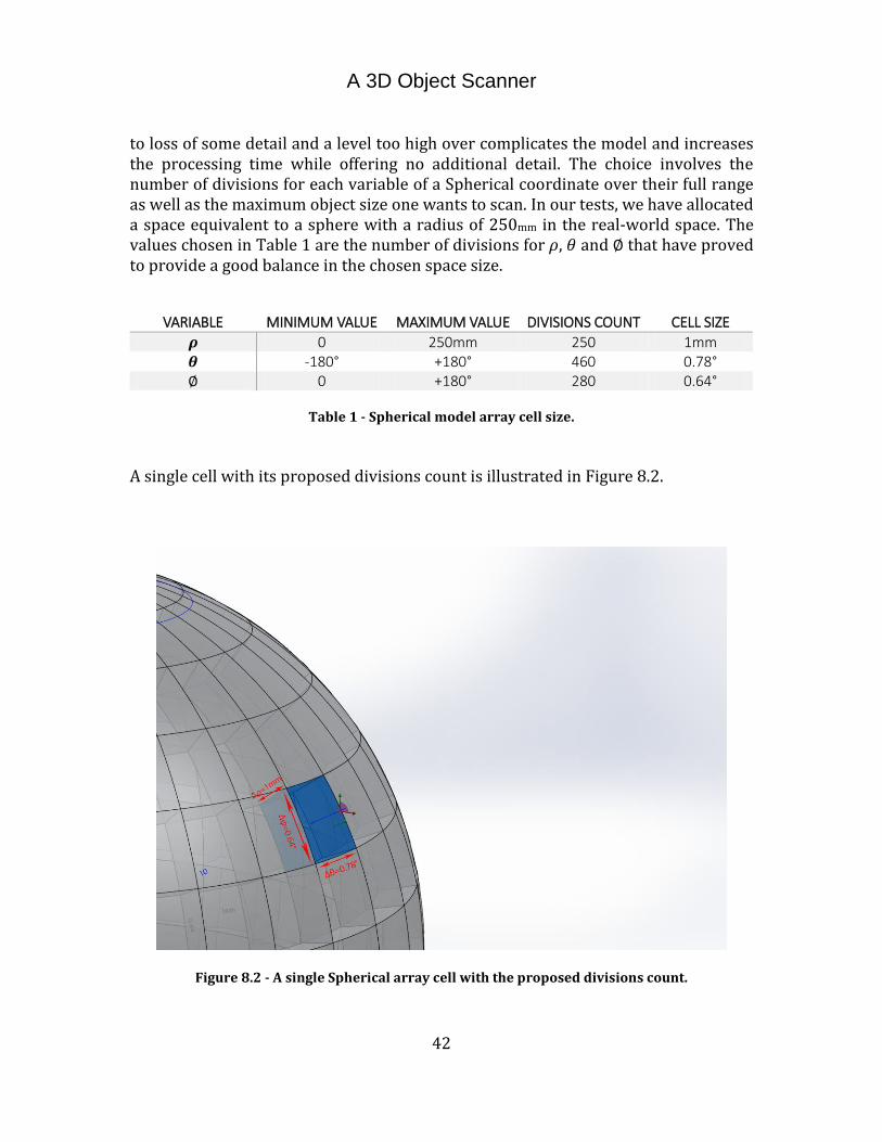
to loss of some detail and a level too high over complicates the model and increases the processing time while offering no additional detail. The choice involves the number of divisions for each variable of a Spherical coordinate over their full range as well as the maximum object size one wants to scan. In our tests, we have allocated a space equivalent to a sphere with a radius of 250mm in the real-world space. The values chosen in Table 1 are the number of divisions for 𝜌, 𝜃 and ∅ that have proved to provide a good balance in the chosen space size.

VARIABLE MINIMUM VALUE MAXIMUM VALUE DIVISIONS COUNT CELL SIZE

𝝆 0 250mm 250 1mm 𝜽 -180° +180° 460 0.78° ∅ 0 +180° 280 0.64°

Table 1 - Spherical model array cell size. A single cell with its proposed divisions count is illustrated in Figure 8.2.

Figure 8.2 - A single Spherical array cell with the proposed divisions count.

A 3D Object Scanner

43

8.1.1 N-Model array

The N-Model array is a Spherical model array, which is used to store the Point Clouds captured in each rotation step at the time scanning is being performed.

Since the occupancy value is increased by one unit every time, it would require only a single bit of memory for every vertex observation! This means, every time a vertex with coordinates of (ρ0, θ0, ϕ0) is observed, the n variable of the array cell struct corresponding to the vertex of such coordinates is incremented by 1. This allows 255 observations of every single vertex which would theoretically allow the storage of a maximum of 255 Point Clouds of rotation steps during the scanning phase which is far more than what we typically need.

Using the idea explained above, the Point Cloud can be stored in real time. Since the unsigned char data type is only 1 byte long, for an array to store a model with a maximum diameter of 50cm, we only need a total memory size estimated according to Equation 6-1 below,

𝑴𝒆𝒎𝒐𝒓𝒚𝒔𝒑𝒉𝒓 = 𝑫𝒔𝒑𝒉𝒓 × 𝟏 = 𝟐𝟓𝟎 × 𝟒𝟔𝟎 × 𝟐𝟖𝟎 × 𝟏 = 𝟑𝟐, 𝟐𝟎𝟎, 𝟎𝟎𝟎 𝒃𝒚𝒕𝒆𝒔 ≅ 𝟑𝟏 𝑴𝑩 (6-1)

As explained before, 31 MB can be used to store a maximum of 255 Point Clouds which is extremely efficient and with today’s Gigabyte memories on computers, it’s only a fraction of the total memory size found on every PC.

8.1.2 M-Model array

The M-Model array is in every aspect similar to the N-Model array but will be filled during the merging phase and holds the final model.

8.1.3 Mapping Spherical coordinates to array index

In order to calculate the flat array index of a voxel’s Spherical coordinates Vs for an array with dimensions of Dρ×Dθ×Dφ, the first step is to calculate an index for each of the dimensions. This can be done using Equations 6-2, 6-3, 6-4, 6-5, 6-6 and 6-7.

𝑉𝑠 = [

𝑉𝑠0

𝑉𝑠1

𝑉𝑠2

] (6-2)

A 3D Object Scanner

44

𝜌𝑖 = {⌊𝑉𝑠0

⌋, 𝑉𝑠0− ⌊𝑉𝑠0

⌋ < ⌈𝑉𝑠0⌉ − 𝑉𝑠0

⌈𝑉𝑠0⌉, 𝑜𝑡ℎ𝑒𝑟𝑤𝑖𝑠𝑒

(6-3)

𝑉′𝑠1

= (𝑉𝑠1+ 𝜋) ×

𝐷𝜃

2𝜋 (6-4)

𝜃𝑖 = {⌊𝑉′

𝑠1⌋, 𝑉′

𝑠1− ⌊𝑉′

𝑠1⌋ < ⌈𝑉′

𝑠1⌉ − 𝑉′

𝑠1

⌈𝑉′𝑠1

⌉, 𝑜𝑡ℎ𝑒𝑟𝑤𝑖𝑠𝑒 (6-5)

𝑉′𝑠2

= 𝑉𝑠2×

𝐷∅

𝜋 (6-6)

∅𝑖 = {⌊𝑉′

𝑠2⌋, 𝑉′

𝑠2− ⌊𝑉′

𝑠2⌋ < ⌈𝑉′

𝑠2⌉ − 𝑉′

𝑠2

⌈𝑉′𝑠2

⌉, 𝑜𝑡ℎ𝑒𝑟𝑤𝑖𝑠𝑒 (6-7)

And finally, the flat array index for the n-model (or similarly m-model) is calculated using Equation 6-8.

𝑖𝑛 = ∅𝑖𝐷𝜌𝐷𝜃 + 𝜃𝑖𝐷𝜌 + 𝜌𝑖 (6-8)

8.1.4 Mapping array index to Spherical coordinates

The inverse conversion of what we calculated in the previous section can easily be calculated using Equations 6-9, 6-10, 6-11 and 6-12. However, the first step is to calculate the individual intermediate coordinates for each dimension.

𝜌′𝑖 = ⌊𝑖𝑛

𝐷𝜌𝐷𝜃⌋ (6-9)

𝜃′𝑖 = ⌊𝑖𝑛−𝜌′𝑖𝐷𝜌𝐷𝜃

𝐷𝜌⌋ (6-10)

A 3D Object Scanner

45

∅′𝑖 = 𝑖𝑛 − 𝜌′

𝑖𝐷𝜌𝐷𝜃 − 𝜃′𝑖𝐷𝜌 (6-11)

𝑉𝑠 = [

𝜌′𝑖𝜃′𝑖𝐷𝜃 − 𝜋

∅′𝑖𝐷∅

] (6-12)

A 3D Object Scanner

46

A 3D Object Scanner

47

Merging

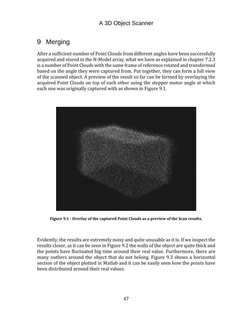
After a sufficient number of Point Clouds from different angles have been successfully acquired and stored in the N-Model array, what we have as explained in chapter 7.2.3 is a number of Point Clouds with the same frame of reference rotated and transformed based on the angle they were captured from. Put together, they can form a full view of the scanned object. A preview of the result so far can be formed by overlaying the acquired Point Clouds on top of each other using the stepper motor angle at which each one was originally captured with as shown in Figure 9.1.

Figure 9.1 - Overlay of the captured Point Clouds as a preview of the Scan results.

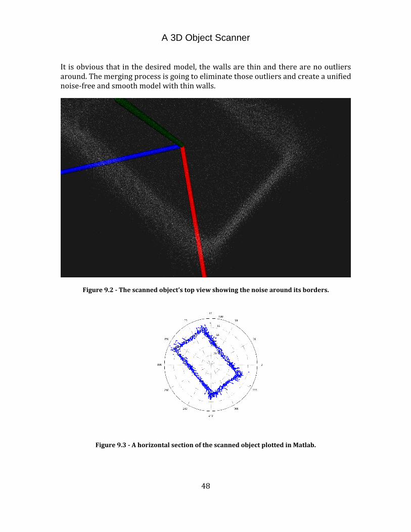
Evidently, the results are extremely noisy and quite unusable as it is. If we inspect the results closer, as it can be seen in Figure 9.2 the walls of the object are quite thick and the points have fluctuated big time around their real value. Furthermore, there are many outliers around the object that do not belong. Figure 9.3 shows a horizontal section of the object plotted in Matlab and it can be easily seen how the points have been distributed around their real values.

A 3D Object Scanner

48

It is obvious that in the desired model, the walls are thin and there are no outliers around. The merging process is going to eliminate those outliers and create a unified noise-free and smooth model with thin walls.

Figure 9.2 - The scanned object’s top view showing the noise around its borders.

Figure 9.3 - A horizontal section of the scanned object plotted in Matlab.

A 3D Object Scanner

49

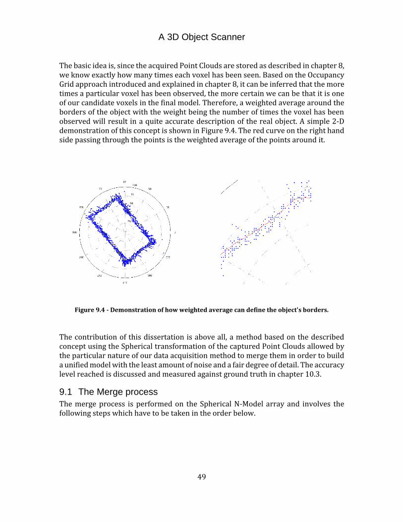
The basic idea is, since the acquired Point Clouds are stored as described in chapter 8, we know exactly how many times each voxel has been seen. Based on the Occupancy Grid approach introduced and explained in chapter 8, it can be inferred that the more times a particular voxel has been observed, the more certain we can be that it is one of our candidate voxels in the final model. Therefore, a weighted average around the borders of the object with the weight being the number of times the voxel has been observed will result in a quite accurate description of the real object. A simple 2-D demonstration of this concept is shown in Figure 9.4. The red curve on the right hand side passing through the points is the weighted average of the points around it.

Figure 9.4 - Demonstration of how weighted average can define the object's borders.

The contribution of this dissertation is above all, a method based on the described concept using the Spherical transformation of the captured Point Clouds allowed by the particular nature of our data acquisition method to merge them in order to build a unified model with the least amount of noise and a fair degree of detail. The accuracy level reached is discussed and measured against ground truth in chapter 10.3.

9.1 The Merge process

The merge process is performed on the Spherical N-Model array and involves the following steps which have to be taken in the order below.

A 3D Object Scanner

50

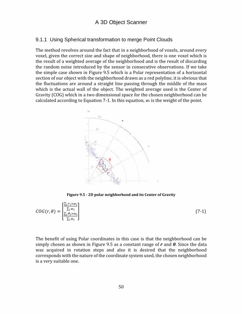
9.1.1 Using Spherical transformation to merge Point Clouds

The method revolves around the fact that in a neighborhood of voxels, around every voxel, given the correct size and shape of neighborhood, there is one voxel which is the result of a weighted average of the neighborhood and is the result of discarding the random noise introduced by the sensor in consecutive observations. If we take the simple case shown in Figure 9.5 which is a Polar representation of a horizontal section of our object with the neighborhood drawn as a red polyline, it is obvious that the fluctuations are around a straight line passing through the middle of the mass which is the actual wall of the object. The weighted average used is the Center of Gravity (COG) which in a two dimensional space for the chosen neighborhood can be calculated according to Equation 7-1. In this equation, wi is the weight of the point.

Figure 9.5 - 2D polar neighborhood and its Center of Gravity

𝐶𝑂𝐺(𝑟, 𝜃) = [

∑ 𝑟𝑖×𝑤𝑖𝑖

∑ 𝑤𝑖𝑖

∑ 𝜃𝑖×𝑤𝑖𝑖

∑ 𝑤𝑖𝑖

] (7-1)

The benefit of using Polar coordinates in this case is that the neighborhood can be simply chosen as shown in Figure 9.5 as a constant range of r and θ. Since the data was acquired in rotation steps and also it is desired that the neighborhood corresponds with the nature of the coordinate system used, the chosen neighborhood is a very suitable one.

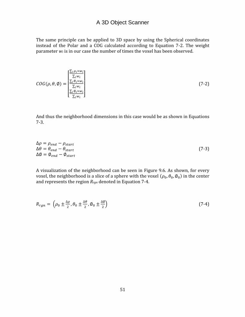
A 3D Object Scanner

51

The same principle can be applied to 3D space by using the Spherical coordinates instead of the Polar and a COG calculated according to Equation 7-2. The weight parameter wi is in our case the number of times the voxel has been observed.

𝐶𝑂𝐺(𝜌, 𝜃, ∅) =

[ ∑ 𝜌𝑖×𝑤𝑖𝑖

∑ 𝑤𝑖𝑖

∑ 𝜃𝑖×𝑤𝑖𝑖

∑ 𝑤𝑖𝑖

∑ ∅𝑖×𝑤𝑖𝑖

∑ 𝑤𝑖𝑖 ]

(7-2)

And thus the neighborhood dimensions in this case would be as shown in Equations 7-3.

∆𝜌 = 𝜌𝑒𝑛𝑑 − 𝜌𝑠𝑡𝑎𝑟𝑡 ∆𝜃 = 𝜃𝑒𝑛𝑑 − 𝜃𝑠𝑡𝑎𝑟𝑡 (7-3) ∆∅ = ∅𝑒𝑛𝑑 − ∅𝑠𝑡𝑎𝑟𝑡

A visualization of the neighborhood can be seen in Figure 9.6. As shown, for every voxel, the neighborhood is a slice of a sphere with the voxel (𝜌0, 𝜃0, ∅0) in the center and represents the region Rrgn denoted in Equation 7-4.

𝑅𝑟𝑔𝑛 = (𝜌0 ±∆𝜌

2, 𝜃0 ±

∆𝜃

2, ∅0 ±

∆∅

2) (7-4)

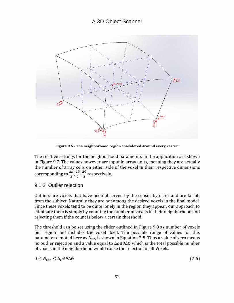
A 3D Object Scanner

52

Figure 9.6 - The neighborhood region considered around every vertex.

The relative settings for the neighborhood parameters in the application are shown in Figure 9.7. The values however are input in array units, meaning they are actually the number of array cells on either side of the voxel in their respective dimensions

corresponding to ∆𝜌

2,∆𝜃

2,∆∅

2 respectively.

9.1.2 Outlier rejection

Outliers are voxels that have been observed by the sensor by error and are far off from the subject. Naturally they are not among the desired voxels in the final model. Since these voxels tend to be quite lonely in the region they appear, our approach to eliminate them is simply by counting the number of voxels in their neighborhood and rejecting them if the count is below a certain threshold.

The threshold can be set using the slider outlined in Figure 9.8 as number of voxels per region and includes the voxel itself. The possible range of values for this parameter denoted here as Nthr, is shown in Equation 7-5. Thus a value of zero means no outlier rejection and a value equal to ∆𝜌∆𝜃∆∅ which is the total possible number of voxels in the neighborhood would cause the rejection of all Voxels.

0 ≤ 𝑁𝑡ℎ𝑟 ≤ ∆𝜌∆𝜃∆∅ (7-5)

A 3D Object Scanner

53

Figure 9.7 - Neighborhood parameters settings.

Figure 9.8 - Outlier rejection settings.

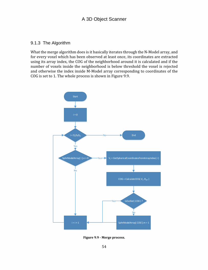
A 3D Object Scanner

54

9.1.3 The Algorithm

What the merge algorithm does is it basically iterates through the N-Model array, and for every voxel which has been observed at least once, its coordinates are extracted using its array index, the COG of the neighborhood around it is calculated and if the number of voxels inside the neighborhood is below threshold the voxel is rejected and otherwise the index inside M-Model array corresponding to coordinates of the COG is set to 1. The whole process is shown in Figure 9.9.

Start

i = 0

i < DρDθDφ

SphrModelArray[ i ].n > 0

Yes

Yes Vs = GetSphericalCoordinatesFromArrayIndex( i )

COG = CalculateCOG( Vs, Rrgn )

IsOutlier( COG ) ?

No

SphrModelArray[ COG ].m = 1i = i + 1

No

EndNo

Yes

Figure 9.9 - Merge process.

A 3D Object Scanner

55

9.1.4 Additional passes

If after fine-tuning the parameters, the result still contain many undesirable voxels or is not smooth enough, one or more additional passes of the same process can significantly smoothen the end results and remove additional unwanted voxels at the cost of discarding some of the wanted voxels as well and decreasing the level of detail. The next chapter will show how changing parameters and additional passes can affect the end results.

A 3D Object Scanner

56

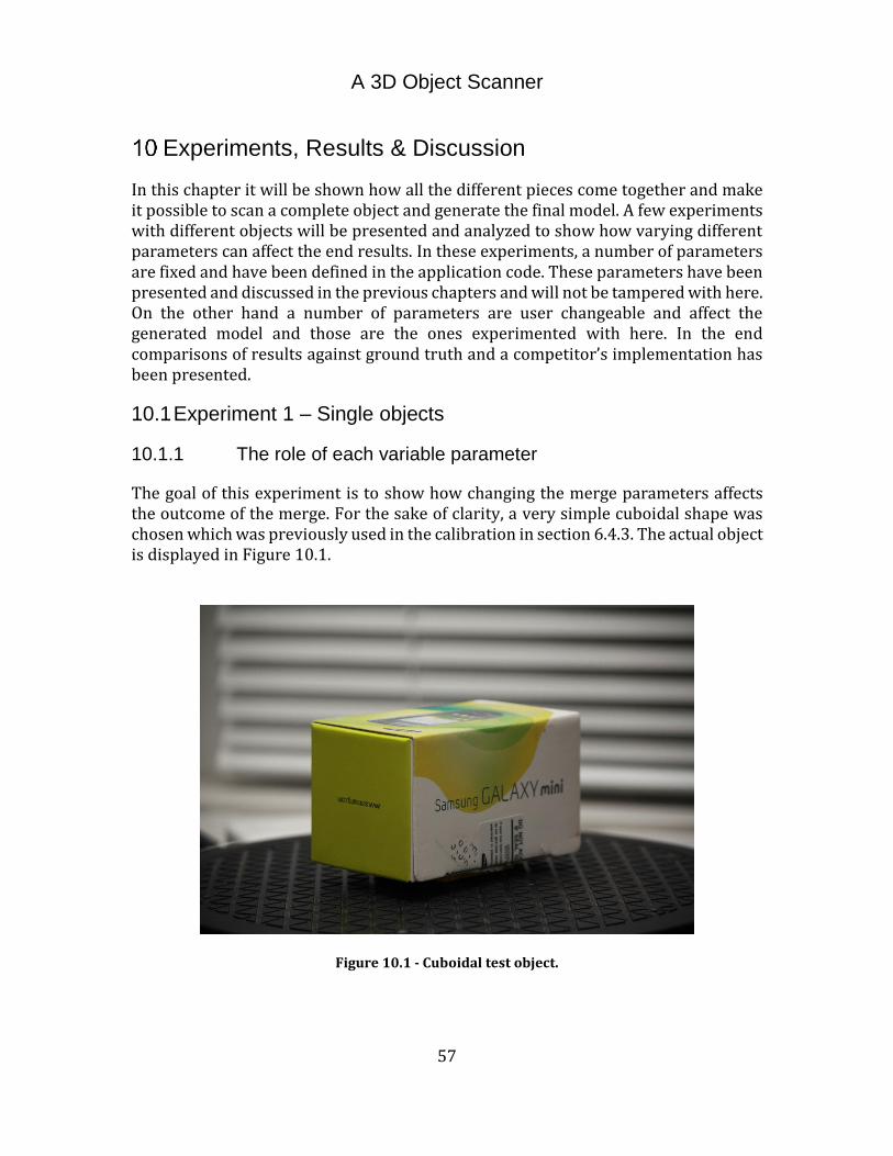
A 3D Object Scanner

57

Experiments, Results & Discussion

In this chapter it will be shown how all the different pieces come together and make it possible to scan a complete object and generate the final model. A few experiments with different objects will be presented and analyzed to show how varying different parameters can affect the end results. In these experiments, a number of parameters are fixed and have been defined in the application code. These parameters have been presented and discussed in the previous chapters and will not be tampered with here. On the other hand a number of parameters are user changeable and affect the generated model and those are the ones experimented with here. In the end comparisons of results against ground truth and a competitor’s implementation has been presented.

10.1 Experiment 1 – Single objects

10.1.1 The role of each variable parameter

The goal of this experiment is to show how changing the merge parameters affects the outcome of the merge. For the sake of clarity, a very simple cuboidal shape was chosen which was previously used in the calibration in section 6.4.3. The actual object is displayed in Figure 10.1.

Figure 10.1 - Cuboidal test object.

A 3D Object Scanner

58

The first step is to scan the object. This is done using the Scan button in the 3DScanner application. The application’s main window is shown in Figure 10.2. And the settings used for this experiment are as displayed in Figure 10.3. The scanning phase took around 4’ 20” and the preliminary result is shown in Figure 10.4.

Figure 10.2 - 3DScanner's main application window.

Figure 10.3 - Settings used in Experiment 1.1.

A 3D Object Scanner

59

Figure 10.4 - Preliminary results of Experiment 1.1.

As seen, the walls of the object are quite thick and very fuzzy. It is evident that the model in its current state is quite unusable.

Phase 1: Initial values

The next step would be to merge the captured Point Clouds in a single model. This is done using the Combine button which performs the procedure explained in chapter 9. Since the goal is to study the effects of parameter variations, the values listed in Table 2 are used as the primary values for the first phase.

SETTING NOTATION VALUE DESCRIPTION RHO RADIUS ∆𝜌/2 5 Rho units of array cells in neighborhood size. THETA RADIUS ∆𝜃/2 1 Theta units of array cells in neighborhood size. PHI RADIUS ∆∅/2 1 Phi units of array cells in neighborhood size. OUTLIER REJECTION THRESHOLD 𝑁𝑡ℎ𝑟 0 Outlier rejection threshold.

Table 2 - Experiment 1.1, Phase 1 parameters.

The merge takes 43” for this phase and the resulting model is shown in Figure 10.5. The result is still very noisy. This is due to the fact that the Rho Radius chosen is too small for the distribution of noise around the actual voxels.

Phase 2: Rho Radius variations

The next phase will show the effect of the Rho Radius variations. As a starting value, the Rho Radius was doubled i.e. it was set to 10.

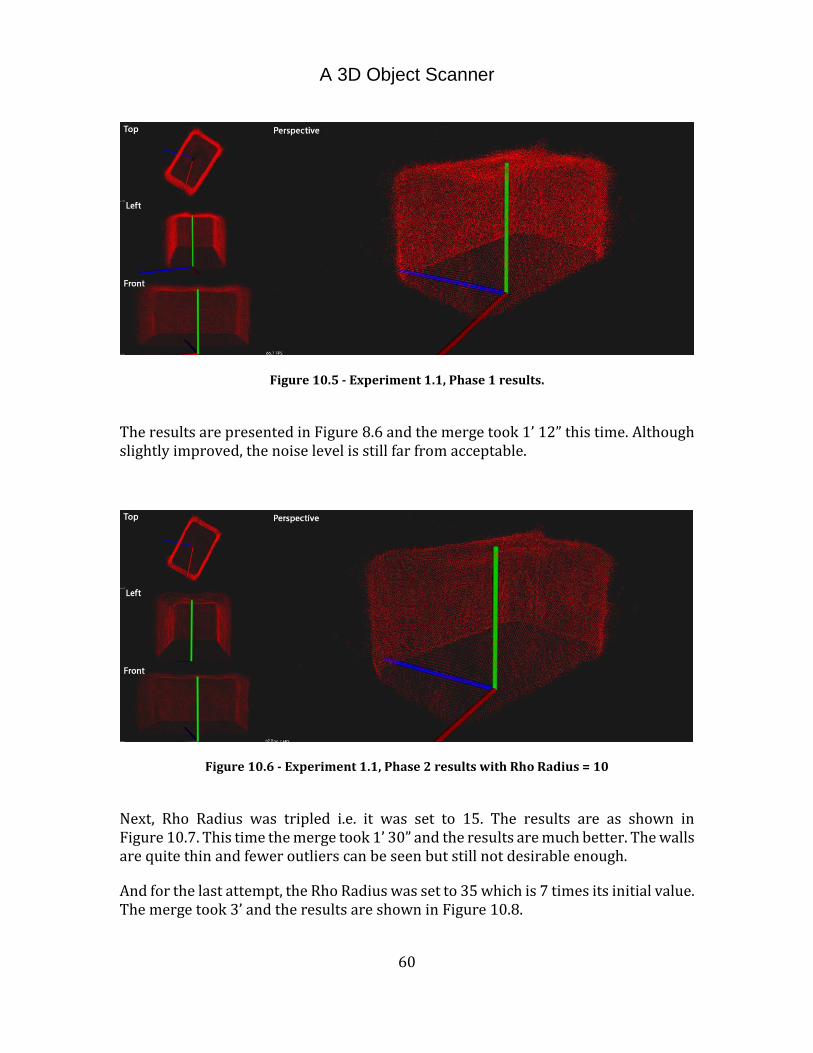
A 3D Object Scanner

60

Figure 10.5 - Experiment 1.1, Phase 1 results.

The results are presented in Figure 8.6 and the merge took 1’ 12” this time. Although slightly improved, the noise level is still far from acceptable.

Figure 10.6 - Experiment 1.1, Phase 2 results with Rho Radius = 10

Next, Rho Radius was tripled i.e. it was set to 15. The results are as shown in Figure 10.7. This time the merge took 1’ 30” and the results are much better. The walls are quite thin and fewer outliers can be seen but still not desirable enough.

And for the last attempt, the Rho Radius was set to 35 which is 7 times its initial value. The merge took 3’ and the results are shown in Figure 10.8.

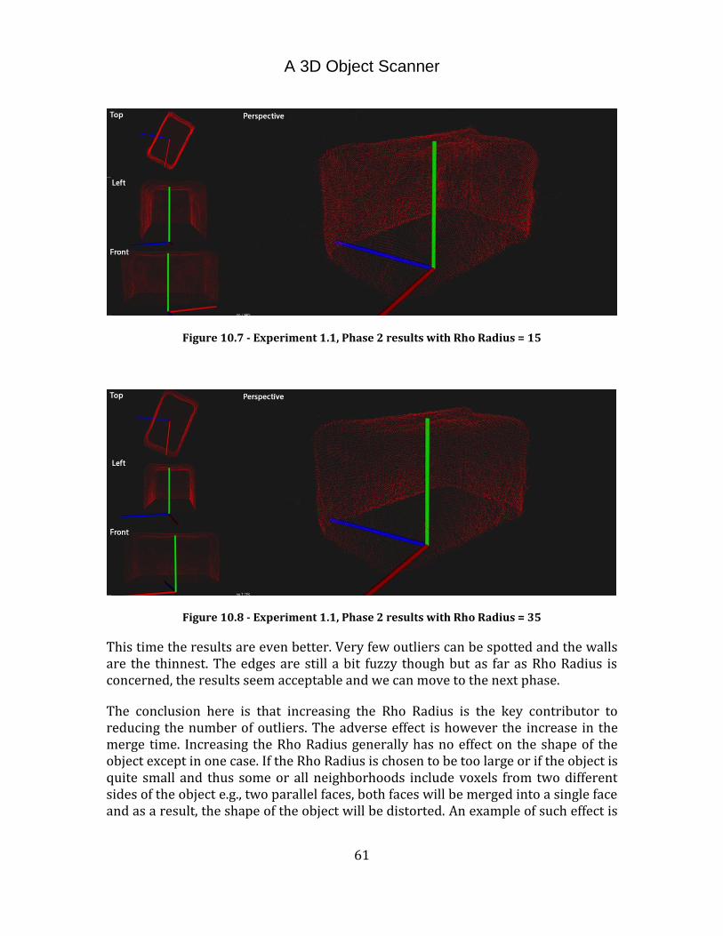
A 3D Object Scanner

61

Figure 10.7 - Experiment 1.1, Phase 2 results with Rho Radius = 15

Figure 10.8 - Experiment 1.1, Phase 2 results with Rho Radius = 35

This time the results are even better. Very few outliers can be spotted and the walls are the thinnest. The edges are still a bit fuzzy though but as far as Rho Radius is concerned, the results seem acceptable and we can move to the next phase.

The conclusion here is that increasing the Rho Radius is the key contributor to reducing the number of outliers. The adverse effect is however the increase in the merge time. Increasing the Rho Radius generally has no effect on the shape of the object except in one case. If the Rho Radius is chosen to be too large or if the object is quite small and thus some or all neighborhoods include voxels from two different sides of the object e.g., two parallel faces, both faces will be merged into a single face and as a result, the shape of the object will be distorted. An example of such effect is

A 3D Object Scanner

62

shown in Figure 10.9 where the object has a thin wall and increasing the Rho Radius results in destroying the wall width.

Figure 10.9 - Possible side effect of Rho Radius increase. a) Rho Radius = 5 b) Rho Radius = 15

Phase 3: Theta and Phi Radius variations

In the previous phase’s results, even in the best of them, the object’s surface does not seem to be flat and has a degree of bumpiness to it. This can be corrected by tweaking Theta and Phi Radiuses. Since the neighborhood must be symmetric, Theta and Phi Radiuses should have the same value and thus changed together.

To get started, a value of 2 is substituted for both Theta and Phi Radiuses and the Rho Radius is kept at 15 since it provides acceptable results while not taking that long. The merge took 3’ 15” and the results are shown in Figure 10.10.

Figure 10.10 - Experiment 1.1, Phase 3 results with Theta and Phi Radius = 2

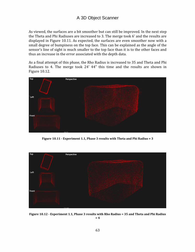
A 3D Object Scanner

63

As viewed, the surfaces are a bit smoother but can still be improved. In the next step the Theta and Phi Radiuses are increased to 3. The merge took 6’ and the results are displayed in Figure 10.11. As expected, the surfaces are even smoother now with a small degree of bumpiness on the top face. This can be explained as the angle of the sensor’s line of sight is much smaller to the top face than it is to the other faces and thus an increase in the error associated with the depth data.

As a final attempt of this phase, the Rho Radius is increased to 35 and Theta and Phi Radiuses to 4. The merge took 24’ 44” this time and the results are shown in Figure 10.12.

Figure 10.11 - Experiment 1.1, Phase 3 results with Theta and Phi Radius = 3

Figure 10.12 - Experiment 1.1, Phase 3 results with Rho Radius = 35 and Theta and Phi Radius = 4

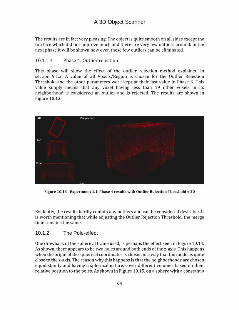
A 3D Object Scanner

64

The results are in fact very pleasing. The object is quite smooth on all sides except the top face which did not improve much and there are very few outliers around. In the next phase it will be shown how even these few outliers can be eliminated.

Phase 4: Outlier rejection

This phase will show the effect of the outlier rejection method explained in section 9.1.2. A value of 20 Voxels/Region is chosen for the Outlier Rejection Threshold and the other parameters were kept at their last value in Phase 3. This value simply means that any voxel having less than 19 other voxels in its neighborhood is considered an outlier and is rejected. The results are shown in Figure 10.13.

Figure 10.13 - Experiment 1.1, Phase 4 results with Outlier Rejection Threshold = 20

Evidently, the results hardly contain any outliers and can be considered desirable. It is worth mentioning that while adjusting the Outlier Rejection Threshold, the merge time remains the same.

10.1.2 The Pole-effect

One drawback of the spherical frame used, is perhaps the effect seen in Figure 10.14. As shown, there appears to be two holes around both ends of the z-axis. This happens when the origin of the spherical coordinates is chosen in a way that the model is quite close to the z-axis. The reason why this happens is that the neighborhoods are chosen equidistantly and having a spherical nature, cover different volumes based on their relative position to the poles. As shown in Figure 10.15, on a sphere with a constant ρ

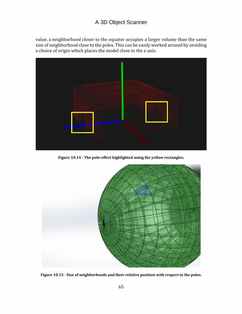
A 3D Object Scanner

65

value, a neighborhood closer to the equator occupies a larger volume than the same size of neighborhood close to the poles. This can be easily worked around by avoiding a choice of origin which places the model close to the z-axis.

Figure 10.14 - The pole-effect highlighted using the yellow rectangles.

Figure 10.15 - Size of neighborhoods and their relative position with respect to the poles.

A 3D Object Scanner

66

10.1.3 A more complex object – The camera

Figure 10.16 - The camera object.

In this experiment a more complex object was chosen, which is a Canon EOS-50D DSLR camera shown in Figure 10.16.

The raw scan results are shown in Figure 10.17. Next, the merge and outlier rejection will be applied to the scanned object and the results will be presented.

Figure 10.17 - Preliminary results of Experiment 1.2

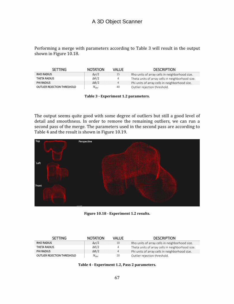
A 3D Object Scanner

67

Performing a merge with parameters according to Table 3 will result in the output shown in Figure 10.18.

SETTING NOTATION VALUE DESCRIPTION RHO RADIUS ∆𝜌/2 15 Rho units of array cells in neighborhood size. THETA RADIUS ∆𝜃/2 4 Theta units of array cells in neighborhood size. PHI RADIUS ∆∅/2 4 Phi units of array cells in neighborhood size. OUTLIER REJECTION THRESHOLD 𝑁𝑡ℎ𝑟 40 Outlier rejection threshold.

Table 3 - Experiment 1.2 parameters.

The output seems quite good with some degree of outliers but still a good level of detail and smoothness. In order to remove the remaining outliers, we can run a second pass of the merge. The parameters used in the second pass are according to Table 4 and the result is shown in Figure 10.19.

Figure 10.18 - Experiment 1.2 results.

SETTING NOTATION VALUE DESCRIPTION

RHO RADIUS ∆𝜌/2 10 Rho units of array cells in neighborhood size. THETA RADIUS ∆𝜃/2 4 Theta units of array cells in neighborhood size. PHI RADIUS ∆∅/2 4 Phi units of array cells in neighborhood size. OUTLIER REJECTION THRESHOLD 𝑁𝑡ℎ𝑟 20 Outlier rejection threshold.

Table 4 - Experiment 1.2, Pass 2 parameters.

A 3D Object Scanner

68

Figure 10.19 - Experiment 1.2, Pass 2 results.

As visible, the object is very smooth with no or very few outliers around but a great number of voxels have been discarded in the second phase. The object however, has still kept a decent level of detail.

10.2 Experiment 2 – Multiple objects

One of the possibilities with the proposed system is to scan multiple objects on the same plate and in one run. The objects and the sensor’s angle however should be in a way that every single part of every object is seen by the sensor in at least one rotation angle. In this experiment this will be put to the test. In order to do that, the objects shown in Figure 10.20 were put on the plate.

Figure 10.20 - Multiple objects.

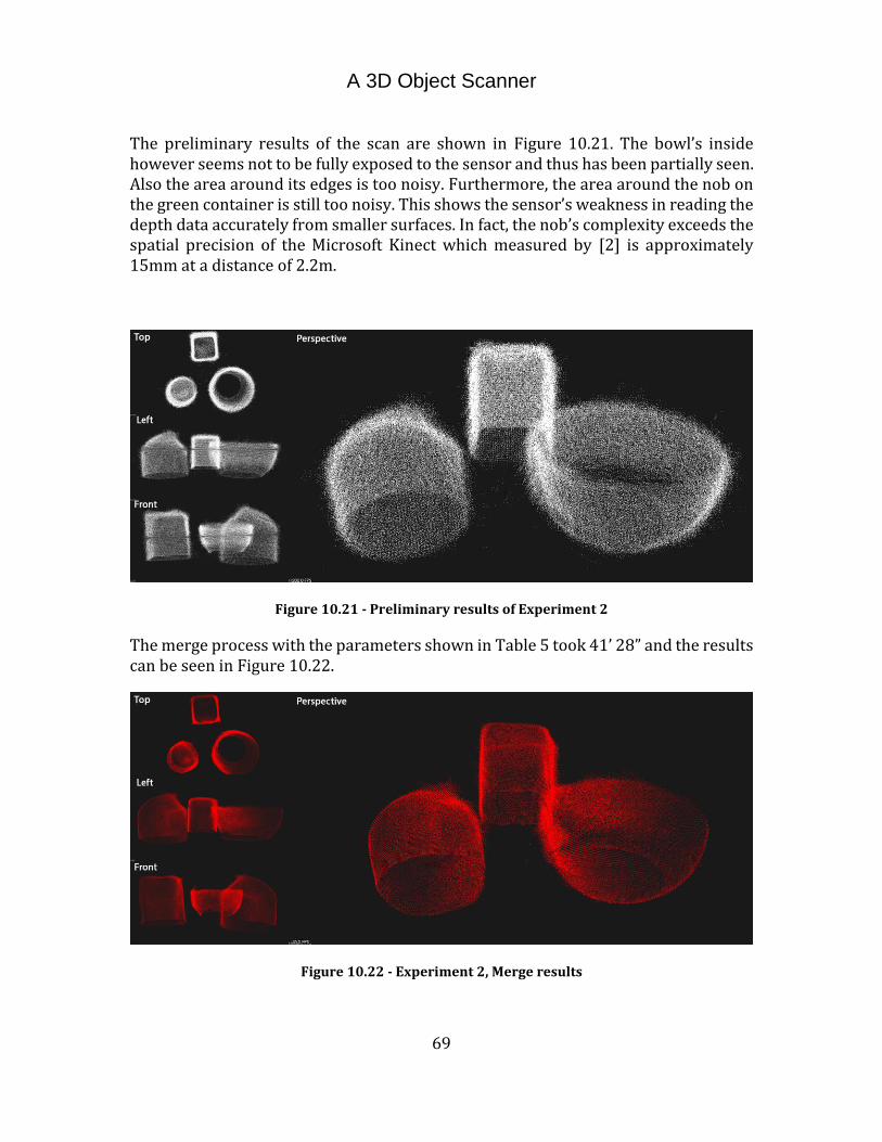
A 3D Object Scanner

69

The preliminary results of the scan are shown in Figure 10.21. The bowl’s inside however seems not to be fully exposed to the sensor and thus has been partially seen. Also the area around its edges is too noisy. Furthermore, the area around the nob on the green container is still too noisy. This shows the sensor’s weakness in reading the depth data accurately from smaller surfaces. In fact, the nob’s complexity exceeds the spatial precision of the Microsoft Kinect which measured by [2] is approximately 15mm at a distance of 2.2m.

Figure 10.21 - Preliminary results of Experiment 2

The merge process with the parameters shown in Table 5 took 41’ 28” and the results can be seen in Figure 10.22.

Figure 10.22 - Experiment 2, Merge results

A 3D Object Scanner

70

SETTING NOTATION VALUE DESCRIPTION

RHO RADIUS ∆𝜌/2 20 Rho units of array cells in neighborhood size. THETA RADIUS ∆𝜃/2 5 Theta units of array cells in neighborhood size. PHI RADIUS ∆∅/2 5 Phi units of array cells in neighborhood size. OUTLIER REJECTION THRESHOLD 𝑁𝑡ℎ𝑟 60 Outlier rejection threshold.

Table 5 - Experiment 2, Merge parameters

The cuboidal object is satisfactorily scanned. The same can be said about the green container disregarding the outlier density around its nob but the bowl is far from good. Perhaps exposure from more angles and specially ones that make it possible for the sensor to see its inside as well could improve the results.

10.3 Evaluation against ground truth

In order to achieve a numerical measure of the accuracy the system is able to offer, a simple test object shown in Figure 10.23 with known dimensions has been used. The object is a simple box of 125mm x 125mm x 51mm dimensions.

Figure 10.23 - Object used to for evaluation against ground truth

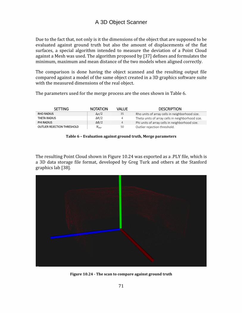
A 3D Object Scanner

71

Due to the fact that, not only is it the dimensions of the object that are supposed to be evaluated against ground truth but also the amount of displacements of the flat surfaces, a special algorithm intended to measure the deviation of a Point Cloud against a Mesh was used. The algorithm proposed by [37] defines and formulates the minimum, maximum and mean distance of the two models when aligned correctly.

The comparison is done having the object scanned and the resulting output file compared against a model of the same object created in a 3D graphics software suite with the measured dimensions of the real object.

The parameters used for the merge process are the ones shown in Table 6.

SETTING NOTATION VALUE DESCRIPTION

RHO RADIUS ∆𝜌/2 35 Rho units of array cells in neighborhood size. THETA RADIUS ∆𝜃/2 4 Theta units of array cells in neighborhood size. PHI RADIUS ∆∅/2 4 Phi units of array cells in neighborhood size. OUTLIER REJECTION THRESHOLD 𝑁𝑡ℎ𝑟 50 Outlier rejection threshold.

Table 6 – Evaluation against ground truth, Merge parameters

The resulting Point Cloud shown in Figure 10.24 was exported as a .PLY file, which is a 3D data storage file format, developed by Greg Turk and others at the Stanford graphics lab [38].

Figure 10.24 - The scan to compare against ground truth

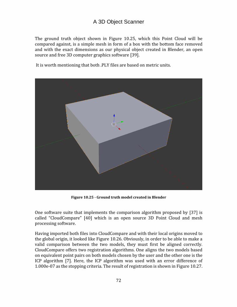
A 3D Object Scanner

72

The ground truth object shown in Figure 10.25, which this Point Cloud will be compared against, is a simple mesh in form of a box with the bottom face removed and with the exact dimensions as our physical object created in Blender, an open source and free 3D computer graphics software [39].

It is worth mentioning that both .PLY files are based on metric units.

Figure 10.25 - Ground truth model created in Blender

One software suite that implements the comparison algorithm proposed by [37] is called “CloudCompare” [40] which is an open source 3D Point Cloud and mesh processing software.

Having imported both files into CloudCompare and with their local origins moved to the global origin, it looked like Figure 10.26. Obviously, in order to be able to make a valid comparison between the two models, they must first be aligned correctly. CloudCompare offers two registration algorithms. One aligns the two models based on equivalent point pairs on both models chosen by the user and the other one is the ICP algorithm [7]. Here, the ICP algorithm was used with an error difference of 1.000e-07 as the stopping criteria. The result of registration is shown in Figure 10.27.

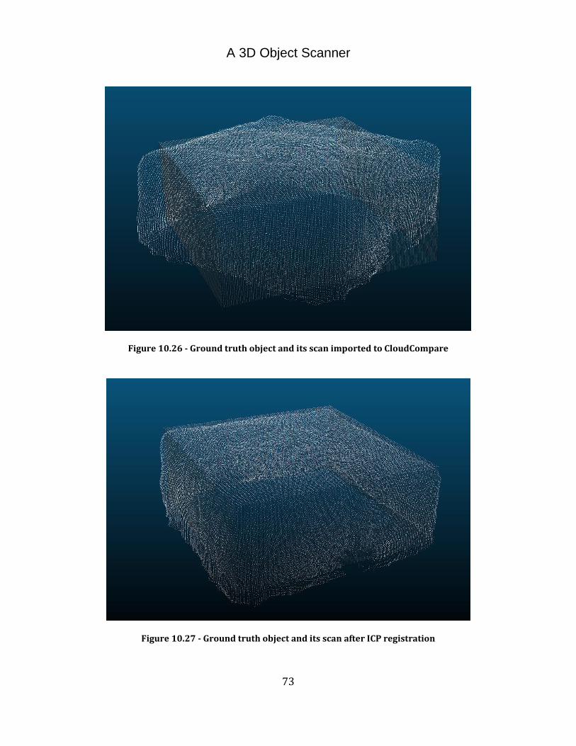
A 3D Object Scanner

73

Figure 10.26 - Ground truth object and its scan imported to CloudCompare

Figure 10.27 - Ground truth object and its scan after ICP registration

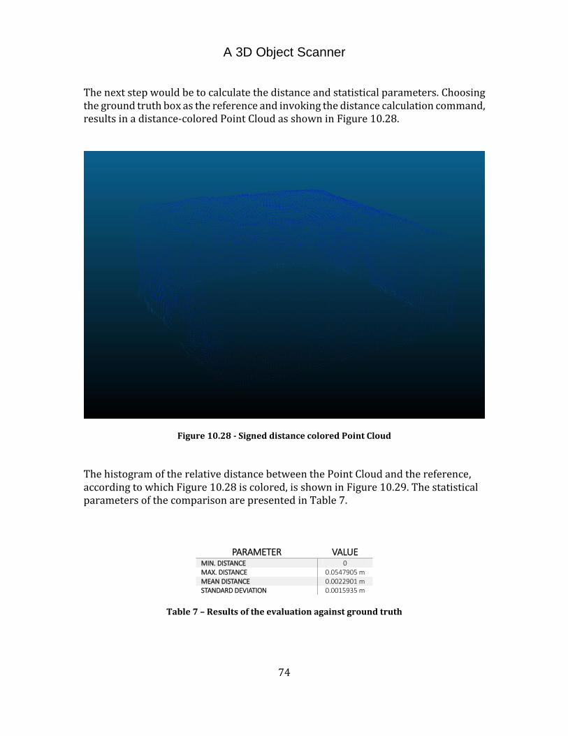
A 3D Object Scanner

74

The next step would be to calculate the distance and statistical parameters. Choosing the ground truth box as the reference and invoking the distance calculation command, results in a distance-colored Point Cloud as shown in Figure 10.28.

Figure 10.28 - Signed distance colored Point Cloud

The histogram of the relative distance between the Point Cloud and the reference, according to which Figure 10.28 is colored, is shown in Figure 10.29. The statistical parameters of the comparison are presented in Table 7.

PARAMETER VALUE MIN. DISTANCE 0 MAX. DISTANCE 0.0547905 m MEAN DISTANCE 0.0022901 m STANDARD DEVIATION 0.0015935 m

Table 7 – Results of the evaluation against ground truth

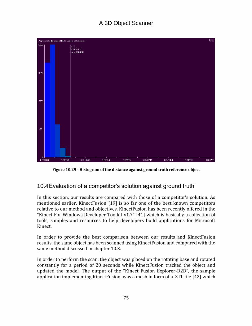
A 3D Object Scanner

75

Figure 10.29 - Histogram of the distance against ground truth reference object

10.4 Evaluation of a competitor’s solution against ground truth

In this section, our results are compared with those of a competitor’s solution. As mentioned earlier, KinectFusion [19] is so far one of the best known competitors relative to our method and objectives. KinectFusion has been recently offered in the “Kinect For Windows Developer Toolkit v1.7” [41] which is basically a collection of tools, samples and resources to help developers build applications for Microsoft Kinect.

In order to provide the best comparison between our results and KinectFusion results, the same object has been scanned using KinectFusion and compared with the same method discussed in chapter 10.3.

In order to perform the scan, the object was placed on the rotating base and rotated constantly for a period of 20 seconds while KinectFusion tracked the object and updated the model. The output of the “Kinect Fusion Explorer-D2D”, the sample application implementing KinectFusion, was a mesh in form of a .STL file [42] which

A 3D Object Scanner

76

is a 3D file format describing surface geometry of an object created by 3D Systems. The result of the scan is displayed in Figure 10.30.

Figure 10.30 - Result of the scan using KinectFusion

Aligned with our ground truth model using the ICP algorithm and an error difference of 1.000e-07 as the stopping criteria, results in what is illustrated in Figure 10.31.

The signed distance colored PointCloud resulting from the distance calculation between the ground truth box as the reference and the scan from KinectFusion is as shown in Figure 10.32 and the statistical parameters of the comparison are presented in Table 8.

PARAMETER VALUE MIN. DISTANCE 0 MAX. DISTANCE 0.0077304 m MEAN DISTANCE 0.0019490 m STANDARD DEVIATION 0.0016144 m

Table 8 – Results of the evaluation of KinectFusion scan against ground truth

A 3D Object Scanner

77

Figure 10.31 - Result of scan using KinectFusion aligned against ground truth model using ICP

Figure 10.32 - Signed distance colored Point Cloud of KinectFusion scan against ground truth

A 3D Object Scanner

78

The histogram of the relative distance between the KinectFusion scan and the ground truth model is illustrated in Figure 10.33.

Figure 10.33 - Histogram of the distance of the KinectFusion scan against ground truth

10.5 Discussion

As shown, the scanner solution provided proves to be able to scan single objects or a number of objects as long as they fit on the rotating plate and do not block each other. The scanner is able to scan simple objects as well as complex ones. Since the most relevant solution close to our work is the KinectFusion [3], [19] performed at Microsoft Research, and it is the state of the art in Kinect Based scanners right now, we have chosen it as a reference to verify and compare our methods and results.

KinectFusion is different to our solution in a few areas. Function wise, where our scanner is aimed at scanning a moving (rotating) object with the sensor being stationary, KinectFusion is aimed at scanning stationary subjects with the sensor being on the move. One other functional difference is that KinectFusion does the scanning and model generation and update in real-time whereas our solution does the scanning in real-time but the model generation is done offline. This puts them in

A 3D Object Scanner

79

two different classes of scanners. Since real-time model generation has never been a goal of our solution, it cannot be considered a weakness.

KinectFusion uses a huge TSDF volume of size (5123) to store the model of the scene and a considerable part of it needs to be updated multiple times per second [19], thus it requires a powerful GPU with parallel computational possibilities. Our implementation is not dependent on any special hardware short for the cheap rotating base.

Perhaps one of the weak sides of our solution is its dependency on correct calibration. The calibration process proposed is mainly visual and this can introduce dimensional but not proportional errors. In other words, the dimensions of the scanned objects might not correspond to their real world dimensions but their proportions will remain intact. KinectFusion is however in no need for any kind of calibration. This is something that can perhaps be improved in the future. One way of doing so might be incorporating the ICP algorithm [7] as done by [3] after passing the raw data through a bilateral filter [43] to reduce the noise.

The storage technique used in our solution being very efficient in terms of speed, size and being closely suitable to the neighborhood traversal needs of our algorithm, can still benefit from some optimization in terms of size. Although 31MB is not much memory on modern computers, using for example Octrees as the data structure of the volume stored much like the approach by [34], can significantly reduce memory size needs.

The main qualitative issue visible is the smooth and curved edges of the object. This is due to the sensor’s higher variance of pixels around contours of objects [2]. The same symptom is clearly visible in the results obtained from KinectFusion as shown in Figure 10.31. One other issue noticeable in Figure 10.31 is that the side faces of the box look slightly pushed in. Since the TSDF volume containing the model is refreshed with each frame upon the entire view frustum of the sensor [19]. This causes the SDF values of the unexposed faces of an object to change as well and thus happens the deformation of the sides. Our solution does not suffer from the same issue.

Another issue, which is a side effect of the spherical coordinates chosen in our method, is the pole-effect discussed in chapter 10.1.2. The reason lies beneath the equidistant sampling of the voxels during the merge process. Although this effect can be avoided by choosing the origin of the frame in a way that would keep the model away from the poles, a better solution would perhaps be a different choice of the neighborhood shape. One possible choice, which would offer a uniform sampling throughout the entire space, is a spherical polyhedron [44]. The most familiar representation of such sampling would be a soccer ball.

A 3D Object Scanner

80

Figure 10.34 - Scanning multiple objects using KinectFusion.

Figure 10.35 - Scanning a detailed object using KinectFusion.

When it comes to scanning multiple objects, KinectFusion seems to function slightly better as it has freedom of movement and obviously has access to more angles than our solution does. The result of one such experiment is shown in Figure 10.34.

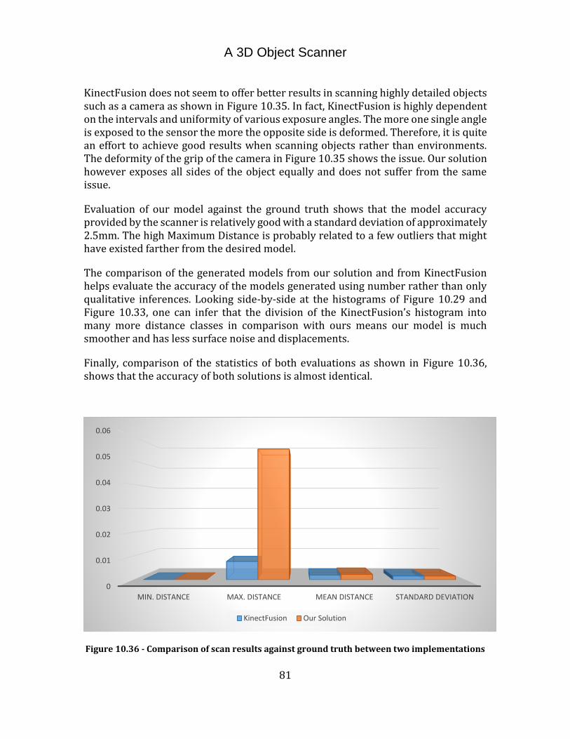
A 3D Object Scanner

81

KinectFusion does not seem to offer better results in scanning highly detailed objects such as a camera as shown in Figure 10.35. In fact, KinectFusion is highly dependent on the intervals and uniformity of various exposure angles. The more one single angle is exposed to the sensor the more the opposite side is deformed. Therefore, it is quite an effort to achieve good results when scanning objects rather than environments. The deformity of the grip of the camera in Figure 10.35 shows the issue. Our solution however exposes all sides of the object equally and does not suffer from the same issue.

Evaluation of our model against the ground truth shows that the model accuracy provided by the scanner is relatively good with a standard deviation of approximately 2.5mm. The high Maximum Distance is probably related to a few outliers that might have existed farther from the desired model.

The comparison of the generated models from our solution and from KinectFusion helps evaluate the accuracy of the models generated using number rather than only qualitative inferences. Looking side-by-side at the histograms of Figure 10.29 and Figure 10.33, one can infer that the division of the KinectFusion’s histogram into many more distance classes in comparison with ours means our model is much smoother and has less surface noise and displacements.

Finally, comparison of the statistics of both evaluations as shown in Figure 10.36, shows that the accuracy of both solutions is almost identical.

Figure 10.36 - Comparison of scan results against ground truth between two implementations

0

0.01

0.02

0.03

0.04

0.05

0.06

MIN. DISTANCE MAX. DISTANCE MEAN DISTANCE STANDARD DEVIATION

KinectFusion Our Solution

A 3D Object Scanner

82

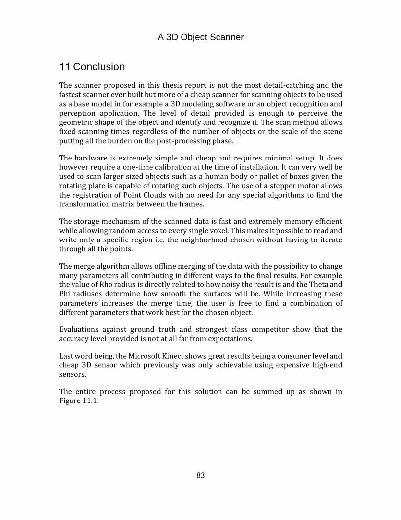
A 3D Object Scanner

83

Conclusion

The scanner proposed in this thesis report is not the most detail-catching and the fastest scanner ever built but more of a cheap scanner for scanning objects to be used as a base model in for example a 3D modeling software or an object recognition and perception application. The level of detail provided is enough to perceive the geometric shape of the object and identify and recognize it. The scan method allows fixed scanning times regardless of the number of objects or the scale of the scene putting all the burden on the post-processing phase.

The hardware is extremely simple and cheap and requires minimal setup. It does however require a one-time calibration at the time of installation. It can very well be used to scan larger sized objects such as a human body or pallet of boxes given the rotating plate is capable of rotating such objects. The use of a stepper motor allows the registration of Point Clouds with no need for any special algorithms to find the transformation matrix between the frames.

The storage mechanism of the scanned data is fast and extremely memory efficient while allowing random access to every single voxel. This makes it possible to read and write only a specific region i.e. the neighborhood chosen without having to iterate through all the points.

The merge algorithm allows offline merging of the data with the possibility to change many parameters all contributing in different ways to the final results. For example the value of Rho radius is directly related to how noisy the result is and the Theta and Phi radiuses determine how smooth the surfaces will be. While increasing these parameters increases the merge time, the user is free to find a combination of different parameters that work best for the chosen object.

Evaluations against ground truth and strongest class competitor show that the accuracy level provided is not at all far from expectations.

Last word being, the Microsoft Kinect shows great results being a consumer level and cheap 3D sensor which previously was only achievable using expensive high-end sensors.

The entire process proposed for this solution can be summed up as shown in Figure 11.1.

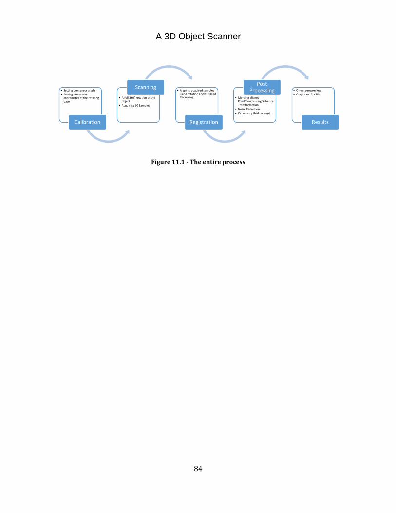
A 3D Object Scanner

84

Figure 11.1 - The entire process

• Setting the sensor angle

• Setting the center coordinates of the rotating base

Calibration

• A full 360° rotation of the object

• Acquiring 50 Samples

Scanning• Aligning acquired samples

using rotation angles (Dead Reckoning)

Registration

• Merging aligned PointClouds using Spherical Transformation

• Noise Reduction

• Occupancy Grid concept

Post Processing • On-screen preview

• Output to .PLY file

Results

A 3D Object Scanner

85

Bibliography

[1] D. Hoiem, "How the Kinect works," Illinois.

[2] M. Andersen, T. Jensen, P. Lisouski, A. Mortensen, M. Hansen, T. Gregersen and P. Ahrendt,

"Kinect depth sensor evaluation for computer vision applications," Department of

Engineering – Electrical and Computer Engineering Aarhus University , 2012.

[3] R. A. Newcombe, S. Izadi, O. Hilliges, D. Molyneaux, D. Kim, A. J. Daviso, P. Kohli, J. Shotton,

S. Hodges and A. Fitzgibbon, "KinectFusion: Real-Time Dense Surface Mapping and

Tracking," 2011.

[4] M. K. Pitt and N. Shephard, "Filtering Via Simulation: Auxiliary Particle Filters," Academic

journal article from Journal of the American Statistical Association, vol. 94, no. 446, 1999.

[5] R. Kalman, "A new approach to linear filtering and prediction problems," Journal of Basic

Engineering 82, no. 1, pp. 35-45, 1960.

[6] M. M. V. S. Paulo Dias, "3D Reconstruction of Real World Scenes Using a Low-Cost 3D Range

Scanner," 2006.

[7] P. J. &. M. N. D. Besl, "A method for registration of 3D shapes," EEE Trans. Pattern Analysis

and Machine Intelligence, 14(2), p. 239–56, 1992.

[8] F. F. A. S. E. A. Christoph Schmalz, "An endoscopic 3D scanner based on structured light,"

Medical Image Analysis 16, pp. 1063-1072, 2012.

[9] I. Daribo, R. Furukawa, R. Sagawa, H. Kawasaki, S. Hiura and N. Asada, "Point Cloud

Compression for Grid-Pattern-based 3D Scanning System," Hiroshima,Tsukuba, Kagoshima.

[10] C.-J. W. C. Z. J.-H. M. Jun-Ting Cheng, "Design of a servo motion system and an image

sampling and processing system on a 3D laser scanner," Int J Adv Manuf Technol 33, p. 1143–

1148, 2007.

[11] U. Qayyum, A. Martin, J. Kim and D. H. Shim, "Omni Viser: 3D Omni Vision - Laser Scanner,"

Wellington, 2012.

[12] J. Tong, J. Zhou, L. Liu, Z. Pan and H. Yan, "Scanning 3D full Human bodies using Kinects".

A 3D Object Scanner

86

[13] T. Nöll, W. Chang, D. Stricker, Y. Cui and A. Vision, "KinectAvatar : Fully automatic body

capture using a single Kinect".

[14] J. Sturm, E. Bylow, F. Kahl and D. Cremers, "Copyme3D : Scanning and printing persons in

3D," Munich, Lund.

[15] W. E. Lorensen and H. E. Cline, "Marching Cubes : A high resolution 3D surface construction

algorithm," New York, 1987.

[16] A. Weiss, D. Hirshberg and M. J. Black, "Home 3D Scans from Noisy Image and Range Data".

[17] D. Anguelov, P. Srinivasan and D. Koller, "Shape completion and animation of people," New

York, 2005.

[18] A. Makadia, A. Patterson IV and K. Daniilindis, "Fully Automatic Registration of 3D point

Clouds," Philadelphia .

[19] D. K. O. H. D. M. R. N. P. K. J. S. S. H. D. F. Shahram Izadi, "KinectFusion: Real-time 3D

Reconstruction and Interaction Using a Moving Depth Camera," in UIST’11, October 16-19,

Santa Barbara, CA, USA, 2011.

[20] B. C. a. M. Levoy, "A volumetric method for building complex models from range images,"

in ACM Trans. Graph, 1996.

[21] H. P. Moravec and A. Elfes, "High resolution maps from angle sonar.," 1985.

[22] H. P. Moravec, "Sensor Fusion in Certainty Grids for Mobile Robots," AI Magazine, vol. 9, no.

2, 1988.

[23] "Kinect for Windows Sensor Components and Specifications," [Online]. Available:

http://msdn.microsoft.com/en-us/library/jj131033.aspx. [Accessed 24 August 2013].

[24] "Kinect," 2013. [Online]. Available: http://en.wikipedia.org/wiki/Kinect.

[25] Landa Electronics, "Datasheet," [Online]. Available:

http://landaelectronic.com/home/1/files/4H4.pdf. [Accessed 15 March 2013].

[26] "Electrokit," [Online]. Available: www.electrokit.com/eibot-board.48383. [Accessed 15

March 2013].

A 3D Object Scanner

87

[27] Microsoft, "Kinect for Windows," [Online]. Available: http://www.microsoft.com/en-

us/kinectforwindows/. [Accessed 15 March 2013].

[28] "About Point Cloud Library (PCL)," [Online]. Available: http://www.pointclouds.org/about/.

[Accessed 15 March 2013].

[29] Pointclouds, "Pointclouds," 2012. [Online]. Available: http://pointclouds.org/. [Accessed 15

March 2013].

[30] "Accelerometer," [Online]. Available: http://msdn.microsoft.com/en-

us/library/jj663790.aspx. [Accessed 24 August 2013].

[31] Microsoft, "Kinect for Windows Programming Guide," [Online]. Available:

http://msdn.microsoft.com/en-us/library/hh855348.aspx. [Accessed 15 March 2013].

[32] A. Elfes, "A Sonar-Based Mapping and Navigation System," 1986.

[33] S. Thrun and A. Bucken, "Integrating Grid-Based and Topological Maps for Mobile Robot

Navigation," Portland, Oregon, 1996.

[34] M. Zeng, F. Zhao, J. Zheng and X. Liu, "A Memory-Efficient KinectFusion Using Octree," in

Computational Visual Media, vol. 7633, Springer Berlin Heidelberg, 2012, pp. 234-241.

[35] "Octree," [Online]. Available: http://en.wikipedia.org/wiki/Octree. [Accessed 25 August

2013].

[36] K. Zhou, M. Gong, X. Huang and B. Guo, "Data-Parallel Octrees for Surface Reconstruction".

[37] P. Cignoni, C. Rocchini and R. Scopigno, "Metro: Measuring Error on Simplified Surfaces,"

vol. 17, no. 2, pp. 167-174, 1998.

[38] "PLY (file format)," [Online]. Available: http://en.wikipedia.org/wiki/PLY_(file_format).

[Accessed 27 August 2013].

[39] "Home of the Blender project - Free and Open 3D creation software," blenderfoundation,

[Online]. Available: http://www.blender.org/. [Accessed 27 August 2013].

[40] "3D point cloud and mesh processing software Open Source project," [Online]. Available:

http://www.danielgm.net/cc/. [Accessed 25 August 2013].

A 3D Object Scanner

88

[41] "Kinect For Windows Developer Downloads," Microsoft, [Online]. Available:

http://www.microsoft.com/en-us/kinectforwindows/develop/developer-downloads.aspx.

[Accessed 28 August 2012].

[42] "STL (file format)," [Online]. Available: http://en.wikipedia.org/wiki/STL_(file_format).

[Accessed 28 August 2013].

[43] C. Tomasi and R. Manduchi., "Bilateral filtering for gray and color," 1998.

[44] P. M. a. E. Schulte, "Abstract Regular Polytopes," 1st ed., Cambridge University Press, pp.

162-165.

A 3D Object Scanner

89

Appendix

A.1 EiBot control commands

The "EM" Command (enable motors)

Format: "EM,<Enable1>,<Enable2><CR>"

To enable a motor driver, set its <Enable> parameter to 1.

To disable a motor driver, set its <Enable> parameter to 0.

For example, "EM,1,0" will enable motor 1 and disable motor 2.

To set the microstep mode of BOTH motor drivers (the same signals go to both drivers, so you can't set them separately) use a value of 1,2,3,4 or 5 for <Enable1>. When you use a value of 1,2,3,4 or 5 for <Enable1>, the <Enable2> parameter is not needed.

When setting microstep values with <Enable1>:

1 will enable both axis in 1/16th step mode (default on boot)

2 will enable both axis in 1/8th step mode

3 will enable both axis in 1/4 step mode

4 will enable both axis in 1/2 step mode

5 will enable both axis in full step mode

Note that any time an SM command is executed, both motors become 'enabled' before the move starts. Thus it is almost never necessary to issue a "EM,1,1" command to enable both motors.

Example: "EM,2" - this command will set both motors in 1/8th step mode

Example: "EM,0,0" - this command will disable both motors (they will then freewheel)

A 3D Object Scanner

90

Example: "EM,1,1" - this command will enable both motors and set them to 1/16th microstep mode.

Return Packet: "OK"

The "SM" Command (stepper motor move)

Format: "SM,<duration>,<axis1>,<axis2><CR>"

<duration> is a value from 1 to 65,535 and is in milliseconds. It represents the total length of time you want this move to take.

<axis1> and <axis2> are values from -32,767 to +32,767 and represent the number of steps for each motor to take in <duration> milliseconds.

If both <axis1> and <axis2> are zero, then a delay of <duration> ms is executed. <axis2> is an optional value, and if it is not included in the command, zero steps are assumed for axis 2.

Use this command to make the motors draw a straight line at constant velocity. The maximum speed that the EBB can generate is 25,000 steps/s. It is helpful to use this command with zeros for both <axis> parameters after moving the pen up or down to give it time to finish moving before starting the next motor move.

Example: "SM,1000,250,-766"

Return Packet: "OK"

Omid Manikhiphone : +46 72 038 61 91 • e-mail : omidontop@gmail.com

Student of Master’s degree in Information Technolgy, Halmstad University, Sweden.Bachelor’s degree in Electronics Engineering, Sadjad University of Technology, Mashhad, Iran.

Behnam Adlkhastphone : +46 73 561 99 82 • e-mail : behnamse@gmail.com

Student of Master’s degree in Information Technolgy, Halmstad University, Sweden.Bachelor’s degree in Software Engineering, Azad University of Tabriz, Iran.

Authors :

PO Box 823, SE-301 18 HalmstadPhone: +35 46 16 71 00E-mail: registrator@hh.sewww.hh.se