-A~ 9 VAUTO F ISRTC AG AT()GANOT N /-1058 EASOCATEIONC NAOF L SAHGUE M D C U OLIVR T A D 1/2

SR-1268 SSC-3ii DOT-CG-928932-A

UNCLASSIFIED IF/O 14/2 N

EEEmohmohmohIEhhmhhhhoshEmhEEhhhohhhhhhhhEEhhmhhohmhhhhEsmhhshmhohhhhEhhhEmhhmhhhhE

_U Hill J 1.0t 16WIfI. LI~ JL L3.6

"1.2 5 11. 11.16 ImlH1m6

MICROCOPY RESOLUTION TEST CHART

MICROCOPY RESOLUTION TEST CHART T NATIONAL BUREAU OF STANDARDS-1963-A

NATIONAL BUREAU OF STANDARDS-1963-A

J

IIfI~ 33li. Q L

1.211 A16

MICROCOPY RESOLUTION TEST CHARTNATIONAL BUREAU OF STANDARDS-1963-A

12

mll I LOI b .L

111.51" . 1111.1 11ELAE.-

/

MICROCOPY RESOLUTION TEST CHART MICROCOPY RESOLUTION TEST CHART

NATIONAL BUREAU OF STANDARDS-1963-A NATIONAL BUREAU OF VTAMNAROG-1963-A

K_ !

SSC- 311(S L-7-27)*1

Oct EVALU ATIO0N O 0F SL- 7SCRATCH-GAUG E DATA

Von&

4c

CT2 4a

aA

ftdimth

4sb f am

SHP CUE OMTE

198

102 8

Id

SHIP STRUCTURE COMMITTEE

The SHIP STRUCTURE COMM4ITTEE Is constituted to prosecute a researchprogram to Improve the hull structures of ships and other marine structuresby an extension of knowledge pertaining to design, materials and methods ofconstruction.

RAd. Clyde T. Lusk, Jr. (Chairman) Mr. J. GrossChief, Office of Merchant Marine Deputy Assistant Administrator for

Safety Comercial DevelopmentU. S. Coast Guard Headquarters Maritime Administration

Mr. P. H. Palermo Mr. J. B. GregoryExecutive Director Chief, Research & Development StaffShip Design & Integration of Planning & Assessment

Directorate U.S. Geological SurveyNaval Sea Systems Comand

Mr. W. N. Hannan Mr. Thomas W. AllenVice President Chief Engineering OfficerAmerican Bureau of Shipping Military Sealift Cosmand

LCdr D. 5. Anderson, U.S. Coast Guard (Secretary)

SHIP STRUCTURE SUBCOMITTEE

The SHIP STRUCTURE SUBCOMMITTEE acts for the Ship StructureComittee on technical matters by providing technical coordination for the

U determination of goals and objectives of the program, and by evaluating andinterpreting the results in terms of structural design, construction andoperation.

U. S. COAST GUARD MILTARY SEALIFT COMAND

Capt. R. L. Brown Mr. Albert AttermeyerCdr. J. C. Card Mr. T. W. ChapmanMr. R. Z. Williams Mr. A. B. StavovyCdr. J. A. Sanial Mr. D. Stein

NAVAL SEA SYSTEMS COMMAND AMERICAN BUREAU OF SHIPPING

Mr. R. Chiu Dr. D. LiuMr. J. B. O'Brien Mr. I. L. SternMr. W. C. SandbergLcdr D. W. Whiddon U. S. GEOLOGICAL SURVEYMr. T. Nomura (Contracts Admin.)

Mr. R. GlangerelliMARITIME ADMINISTRATION Mr. Charles Smith

Hr. N. 0. Homer INTERNATIONAL SHIP STRUCTURES CONGRESSDr. R;. M. MacleanMr. F. Seibold Mr. S. G. Stiansen - LisonMr. M. Touma

AMERICAN IRON & STEEL INSTITUTE'

NATIONAL ACADEMY OF SCIENCES Mr. R. H. Stere - LiaionSHIP RESEARCH COMMITTEE

Mr. A. Dudley Haff - Liaison STATE UNIV. OF NEW YORK MARITIME COLLEGE

Mr. R. W. Rusks - Liaison Dr. W. R. Porter - Liaison

SOCIETY OF NAVAL ARCHITECTS & U. S. COAST GLARD ACADEISY

MARINE ENGINEERS LCdr R. G. Vorthman - Liaison

Mr. A. B. Stavovy - Liaison U. S. NAVAL ACADEMY

Dr. R. Battacharyya - Liaison• WELDING RESEARCH COUNCIL

Mr. K. H. Koopman - Liaison U. S. PERCHAWi 14ARINE ACAI)ENY

Dr. Chin-Sea Kin - Liaison

L

Member Agencies: Address Correspondence to:

,M/iled States Comma Gurd Secretary, Ship Structure Committeev/ See Satema Commend U.S. Coast Guard Headquarters,(G-M/TP 13)Mitery ASmift Commend tnO Washington, D.C. 20593

Mwritime AdministrationUnted Ste ooloIcal Survey

Amerkan Bureau of Ipp/ngAn Interagency Advisory Committee

Dedicated to Improving the Structure of Ships SR-1 268

1981

This report is one of a group of Ship Structure CommitteeReports which describe the SL-7 Instrumentation Program. Thisprogram, a Jointly funded undertaking of Sea-Land Service, Inc., theAmerican Bureau of Shipping and the Ship Structure Committee, representsan excellent example of cooperation between private industry, classificationauthority and government. The goal of the program is to advance under-standing of the performance of ships' hull structures and the effective-ness of the analytical and experimental methods used in their design.While the experiments and analyses of the program are keyed to the SL-7Containership and a considerable body of the data developed relatesspecifically to that ship, the conclusions of the program will be com-pletely general, and thus applicable to any surface ship structure.

The program includes measurement of hull stresses, accelerationsand environmental and operating data on the S.S. Sea-Land McLean,developmt and installation of a microwave radar wavemeter for meas-uring the seaway encountered by the vessel, a wave tank model studyand a theoretical hydrodynamic analysis which relate to the wave in-duced loads, a structural model study and a finite element structuralanalysis which relate to the structural reponse,-and installation oflong-term stress recorders on each of the eight.vessels of the class.In addition, work is underway to develop the initial .correlations ofthe results of the several program elements.

Results of each of the program elements are being made availW>'.-

through the National Technical Information Service, each identifiedan SL-7 number and an AD- number. A list of all SL-7 reports availi 'to date is included in the back of this report.

-This report documents the evaluation of the long-termstress Yer

Clyd T u* m. Rear Admiral, U.S. Coast Guard

Chairman, Ship Structure Committee

.9,

Technical Report Documentation Pago. Report No. 2. G.m,.nt A o N 3. R..p...,, Catalog N..

SSC-311, 4 ~ A/cc 5 _ ___ __ _

4. T-tle and Subt.l(" 5. Repo, Dote

nx A IO7 OF SL-7 S'6.ACH GAGE 'DATA 19816. Perforng gO.anzaton Code

"_ _ __"_ _ _ _ _ _ _ 8. Peroeming Organization Reort No.

"- ." 7. Author's )

". J. C. Oliver, with Contributions by .&K. Ochi I SR- 1268

9. Performing Orgonzoten Name arao Addeass 10 Wnk Unt No. (TRAISI

Giannotti & Associates, Inc.Annapolis, !I. 11. Cont.,, a, Giont No.

DOT-03-920932-A13. Type of Repot and Pe,,od Coveed

Soo12. sp-,e,- Agency Nor, and Addres,,,, FINiAL

U.S. Coast GuardOffice of Merchant Marine Safety )4 sli....... Agergy CodeWashington, D.C. 20593 G-M

IS. Supelementey Note's

The U.S.C.G. acts as the contracting office for the Ship Structure Camlittee

--- lr7 This report assesses the value and application potential of the SL-7 scratch-gauge data base. The principal advantage of the mechanical extreme-stress recordersis large quantities of inexpensive data. Their drawbacks are that contributionsfrom different load sources cannot be separated; contributions frum torsional, lateraland vertical bending cannot be separated; and t!here is no reasonable way to distin-

I quish between hogging and sagging response. Howaver, when the scratch-gauge dataand electrical strain-gauge data from a second operational season aboard the McLEAN

I.were correlated, a clparison between the form of the curves showed good agreement.Several statistical models were found to describe the data well enough to be

used as a basis for statistical infexence beyond the range of measured values. TheType-I Extreme-Value distribution, the Weibull distribution, and a four-parameterdistribution proposed by i. K.- Ohi satisfactorily represent the data in most cases.

. .Docment is available to the U.S.Public

tlrougih the National Technical Informa-Extreme Stress Scratch Gauge tion Service, Springfield, VA 22161

,19. Security CIoss, . (of thi, #*ot) JO. Security Classi. (of thes page) 21. No. of Page. 22. Pt.ce

UiCLASSIFIZ UNcIASSIFIED I 108

* Form DOT F 1700.7 (8-72) Reproduction of completed page authorizedI

j OR

LI His J 111ll o l I m 1111 0 ...61hl l

I ~I iii ii II isI Ui a ef. l-d -

Oldlo

13

U 1 3iv

CONTENTS

PAGE

1.INTRODUCTION.................. . . ... . .. .. .. .. .. .. ... 1

1.1 Background and Objectives...... ... . .. .. .. .. .. ... 1

1.2 Organizat oeore ort. . .. .. .. .. ........ 2

2. INSTRUMENTATION AND PROCEDURE .. .. ........ ........ 3

2.1 Measurement Phenomena. .. ......... ......... 3

2.2 Measurement Process - Instrumentation and Data Collection 3

2.3 Measurement-Generating Process. .. .. ............. 7

2.4 Experimental Errors. .. .......... ......... 8

2.5 Analysis of the Data: Procedure .. .. ......... ... 11

2.6 Port vs. Starboard Gauge Data. .. ......... ..... 12

2.7 Remarks. .. ......... ................ 13

3. CORRELATION WITH STRAIN GAUGE DATA. .. ........ ...... 14

3.1 Linear Regression,.. .. .................. 15

3.2 Hull Structural Analysis. .. .. ............... 16

3.3 Comparison of Calibration Data................17

3.4 Remarks. .. ...................... ...... 18

4. TYPE IEXTREME VALUE MODEL .. .. ................. 19

4.1 Statistical Models. .. .. ............ .. ... 19

4.2 Data Analysis .. .. ........ ............ 21

4.3 Examination of the IdenticallyDistributed Condition. .31

4.4 Examination of the Independence Condition. .. ....... 31

4.5 Remarks................... ....... 39

V

p- --

PAGE

5. OTHER STATISTICAL MODELS ........ ..................... ... 43

5.1 Four-Parameter Expression Proposed by M. K. Ochi ... ....... 43

5.2 Log-Normal Distribution ....... ................... ... 44

5.3 Peibull Distribution (2-parameter) ...... .............. 44

5.4 Type-III Extreme Value Distribution .... ............. ... 45

6. SCRATCH GAUGES: AN ALTERNATIVE TO ELECTRICAL STRAIN GAUGES. . . . 48

6.1 Comparison of Extrapolations Based on Electrical and ..... ... 48Mechanical Strain Measurements

6.2 Remarks ........... ........................... .. 52

7. MISCELLANEOUS APPLICATIONS ....... .................... ... 53

7.1 Mean Stress .......... ......................... ... 53

7.2 Short-Term Statistics ....... ................... .. 55

7.3 Effects of Corrosion.... ...... ................... ... 59

8. EVALUATION OF SCRATCH-GAUGE PROGRAM WITHIN THE CONTEXT OF ........ 60PROBABILISTIC LOAD AND RESPONSE PREDICTION

8.1 Long-Term Prediction Based on Conditional Probabilities . . . 61of Short-Term Loads

8.2 Short-Term Load Prediction Based on Lifetime Extreme Events 65

8.3 Philosophical Perspective .................. 66

9. UTILITY OF THE SCRATCH-GAUGE DATA ...... ................. ... 68

9.1 Extrapolation of Statistical Model .... .............. ... 68

9.2 Validation of Long-Term Prediction Methods ............. ... 71

9.3 Validation of Short-Term Prediction Methods .......... .. 72

9.4 Long-Term Record of Mean Stress ...... .............. ... 72

10. CONCLUSIONS AND RECOMMENDATIONS ...... ................. .... 73

10.1 Summary and Conclusions ........ ................. .. 73

10.2 Recommendations ......... ....................... ... 75

vi

LIST OF FIGURES

FIGURE TITLE PAGE

2-1 General Process of an Engineering Investigation ... ...... 4

2-2 N.C.R.E. - Maximum Reading Strain Gauge Recorder ......... 5

2-3 Ship Gauge Location (from ref. 1) ...... ............. 5

2-4 Component Layout (from ref. 1) ........ ............. 5

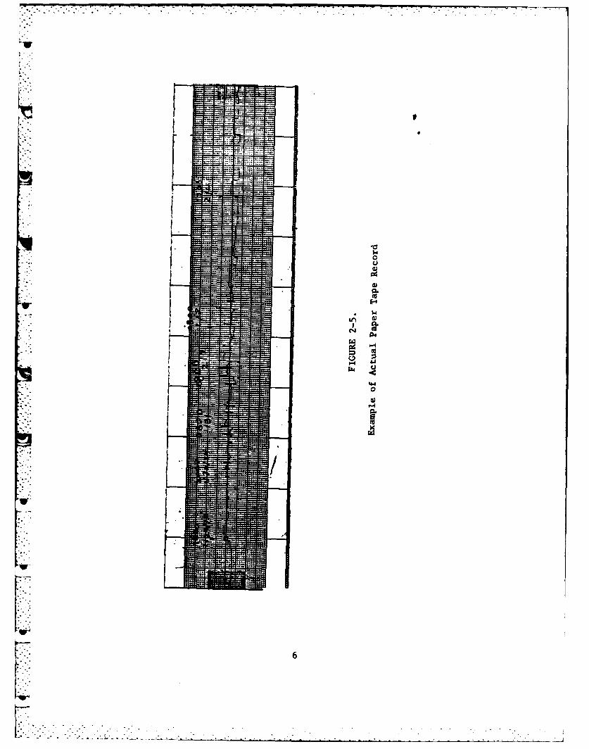
2-5 Example of Actual Paper Tape Record. ............ 6

2-6 Illustration of Scratch Mark Equivalent to Complex..... 8Time History of Stress

2-7 Miscellaneous Details of Scratch Records ..... .......... 9

2-8 Digitizing Tablet and Four-Button Cursor Used for . . . . 12Remeasurement

1

3-1 Ratio of Scratch-Gauge Stress to Strain-Gauge (LVB) . . . . 17Stress

4-1 Several Examples of Nonlinear Plots .... ............ ... 20

4-2a Data Year 1 - Atlantic - Type 1 Extreme Value ......... ... 22

4-2b Data Years 1 and 2 - Atlantic - Type 1 Extreme-Value Fit. 22

4-2c Data Years 1, 2 and 3 - Atlantic - Type 1 Extreme-Value Fit 23

4-2d Data Years 1, 2, 3 and 4 - Atlantic - Type 1 Extreme- . . . 23Value Fit

4-2e Summary Grand Total - Atlantic - Type 1 Extreme-Value Fit 24

4-3a Data Year 1 - Pacific - Type 1 Extreme-Value Fit ......... 25

4-3b Data Years 1 and 2 - Pacific - Type 1 Extreme-Value Fit . 25

4-3c Data Years 1, 2 and 3 - Pacific - Type 1 Extreme-Value Fit. 26

• I 4-3d Data Years 1, 2, 3 and 4 - Pacific - Type 1 Extreme-.... 26

Value Fit

4-3e Summary Grand Total - Pacific - Type 1 Extreme-Value Fit.. 27

4-4 Comparison of Scratch-Gauge Data to Type-I Extreme- .. .... 28Value Probability Density Function for Summary GrandTotal Pacific

vii

FIGURE TITLE PAGE

4-5 Atlantic Statistical Models Yearly Accumulations -. .... 29ist Five Years - Type 1 Extreme-Value Fit

4-6 Pacific Statistical Models Yearly Accumulations -. .... .29

1st Five Years - Type 1 Extreme-Value Fit

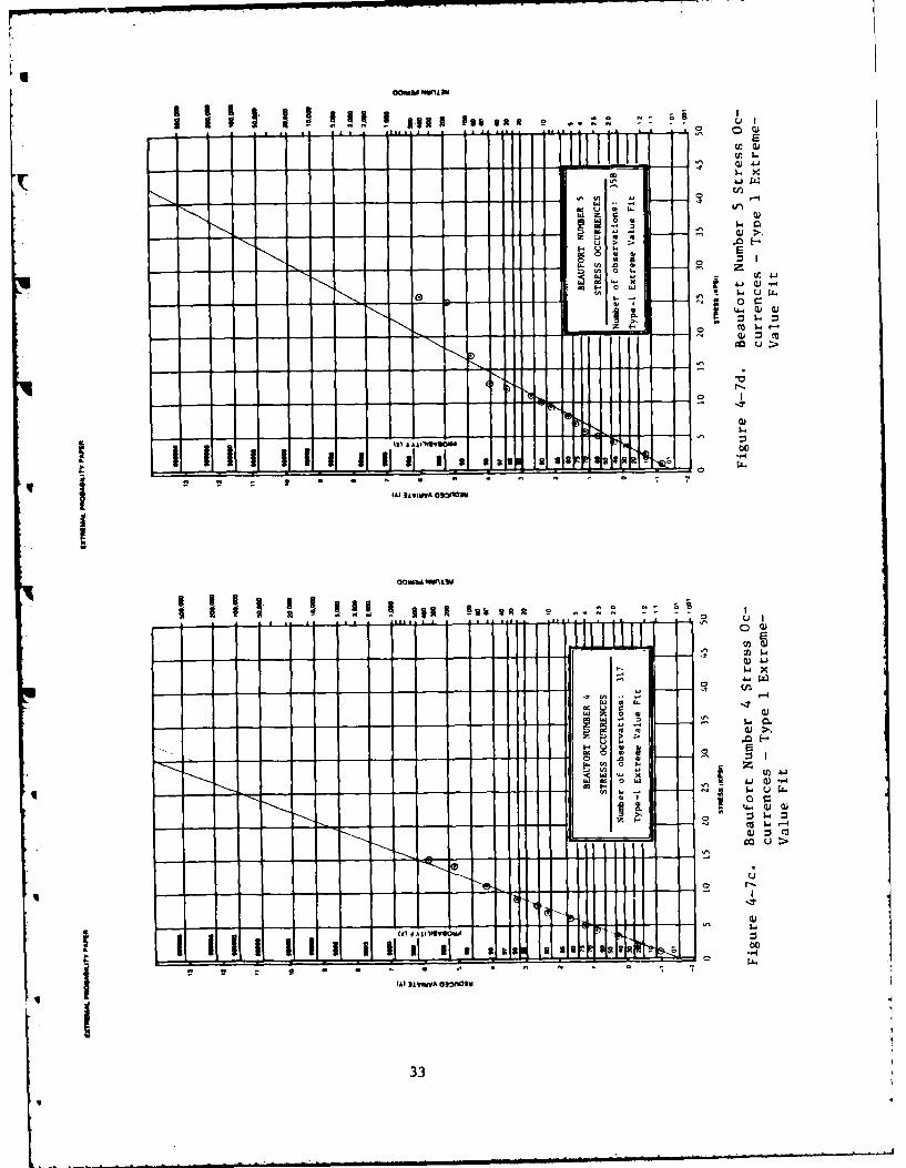
4-7a Beaufort Number 2 Stress Occurrences - Type 1 Extreme-... 32Value Fit

4-7b Beaufort Number 3 Stress Occurrences -Type 1 Extreme-... 32Value Fit

4-7c Beaufort Number 4 Stress Occurrences - Type 1 Extreme-... 33Value Fit

4-7d Beaufort Number 5 Stress Occurrences - Type 1 Extreme-... 33Value Fit

4-7e Beaufort Number 6 Stress Occurrences - Type 1 Extreme-... 34Value Fit

4-7f Beaufort Number 7 Stress Occurrences - Type I Extreme-... 34Value Fit

4-7g Beaufort Number 8 Stress Occurrences- Type 1 Extreme-... 35Value Fit

4-7h Beaufort Number 9 Stress Occurrences - Type 1 Extreme-... 35Value Fit

4-71 Beaufort Number 10 Stress Occurrences - Type 1 Extreme; . . 36" Value Fit

4-7j Beaufort Number 11 Stress Occurrences - Type 1 Extremei . . 36

Value Fit

4-8a Extreme Value 8-Hour Intervals - Type 1 Extreme-Value Fit . 37

4-8b Extreme Value 16-Hour Intervals - Type 1 Extreme-Value Fit. 37

4-8c Extreme Value 24-Hour Intervals - Type 1 Extreme-Value Fit. 38

4-8d Composite of Type-I Extreme-Value Model Fits to 8 ...... ... 3816 and 24 Hour Maxima of Voyages 1 - 37, McLEAN,Starboard Scratch Gauge

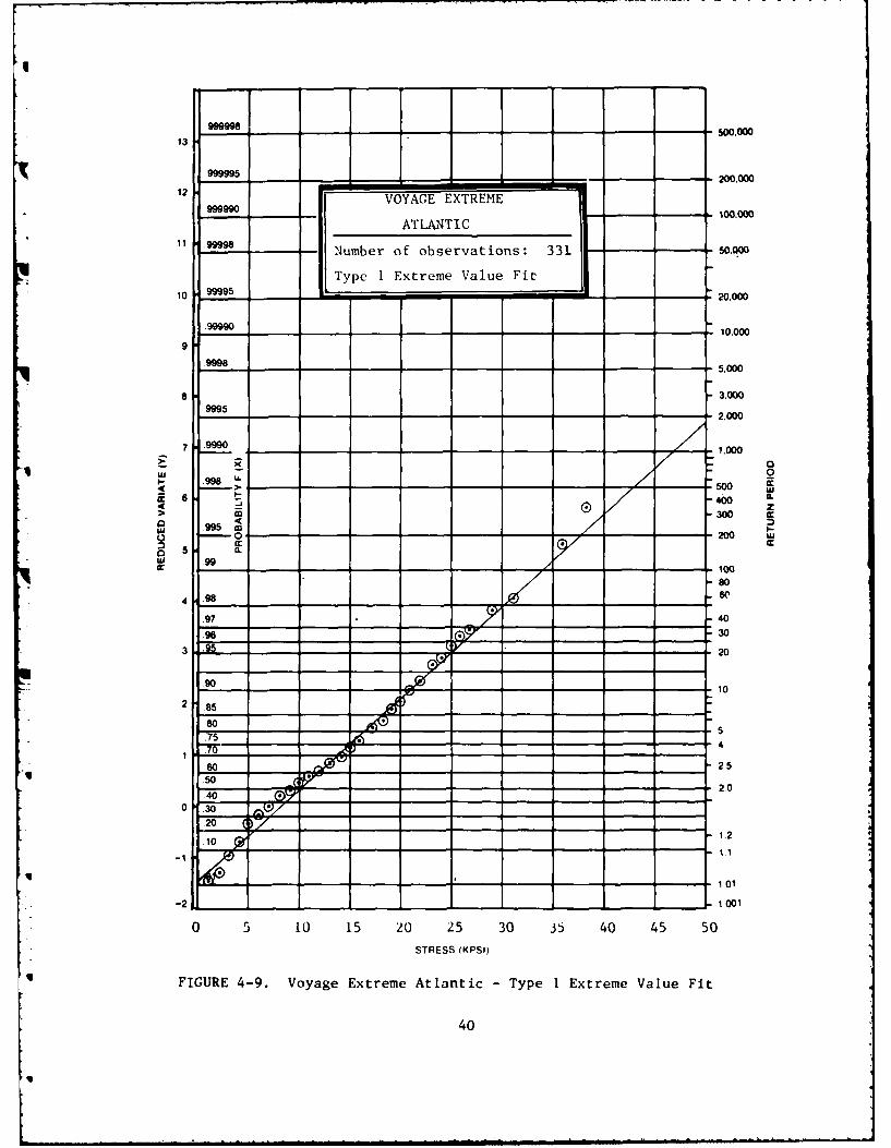
4-9 Voyage Extreme Atlantic - Type 1 Extreme-Value Fit ........ 40

4-10 Voyage Extreme Pacific - Type 1 Extreme-Value Fit ....... 41

V.viii

FIGURE TITLE PAGE

5-1 4-Parameter Distribution Proposed by Ochi: ........... ... 44Atlantic Summary Total Fit

5-2 Atlantic and Pacific Summary Data Plotted on ........... ... 45Probability Paper

5-3 Weibul Fit ....... ....................... ... 46

5-4 Type-III Fit of Voyage Maxima Pacific - All Voyages . . . . 47

6-1 Long-Term Trend on Longitudinal Vertical Bending Stress 49for McLEAN based on Second Operational Season, Voyages25 - 37

6-2 McLEAN Second Operational Season - Type-i Extreme-Value . . 51Fit

7-1 Probability Density Function of Random Variable n as a... 56Function of Bandwidth Parameter c

7-2 Histogram of Peak-to-Trough Stress'vs. Beaufort Number.. 57for Voyages 1 - 37, McLEAN, Starboard Scratch Gauge

-' 9-1 Number of Storm Days at Utsira Each Year from 1920 to . . . 691974 (35)

ix

...

TABLE OF TABLES

TABLE TITLE PAGE

2-1 Comparisons of Scratch-Gauge Data McLEAN Port vs ......... 13Starboard Gauges (Max Peak-to-Trough Stress-KPSI)

3-1 Statistical Correlations - Scratch-Gauge Data vs ......... 15Electrical Strain-Gauge Data - McLEAN

3-2 Correlations from Static Structural Calibration of Ship. . 17Response Instrumentation System - Rotterdam, Holland,9-10 April 1973

4-1 Long-Term Estimates Using Type-I Extreme-Value Distribution. 28for Yearly Accumulations of Scratch Data

4-2 Parameters of Type-I Extreme Value Distribution for Yearly . 30.Accumulations of Scratch Data

6-1 Comparison of Long-Term Estimated Stress Values from .... 50Scratch and Electrical Strain Gauge by Fitted Type-IExtreme Value Distribution - McLEAN - Second Season

7-1 Mean Stress as Derived from Scratch-Gauge Paper Tape - . . 54McLEAN Starboard Gauge

7-2 Evaluation of the Postulate that the Most Severe Weather . 58is Always Associated with the Maximum Strains

8-1 Expressions for Distributions of m- used in Various .... 63Long-Term Prediction Methods o

X

1. INTRODUCTION

1.1 Background and Objectives

Previous Ship Structure Committee projects attempting toestablish load criteria on a probabilistic basis indicated that life-time extreme loads could not yet be predicted with confidence. Inorder to acquire this confidence, mechanical extreme-stress gaugeswere installed on eight SL-7 ships: the SEA-LAND McLEAN, GALLOWAY,COMMERCE, EXCHANGE, TRADE, FINANCE, MARKET, and RESOURCE. The scratchgauge, unattended and continuously running, records the maximum tominimum stress excursion in a four-hour period. Two scratch gaugeswere installed in the McLEAN on October 7, 1972, and the seven otherSL-7 containerships were installed with a single gauge as they weredelivered to their owners. In the first five years of operation,over twenty "ship-years" of data were recorded on paper tape in theform of 36000 + records. The data are presented in histogram form byFain and Booth in SSC-286 (I)t and represent a substantial measure-ment and reduction effort.

This project assesses the value and application potential of thedata base. Specifically, the three-fold objective of the presentproject is to evaluate SL-7 scratch-gauge data as a basis for extreme-load prediction, to determine correlations with SL-7 electricalstrain-gauge data, and to recommend when and how many scratch gaugescan be recovered for placement aboard other ships.

Although the data presented as histograms in SSC-286 form thebasis of the present study, remeasurement and data reduction of someoriginal scratch records were necessary to carry out many of theanalyses. It is not within the scope of this investigation, however,to remeasure, reduce and reprocess the data in bulk.

A scratch-gauge instrumentation program is not without precedent.The Naval Construction Research Establishment (NCRE) of Dunfermline,Fife, United Kingdom, (now AMTE) outfitted over sixty British war-ships of various classes with simple maximum reading mechanicalstrain gauges. The approaches used in that particular program aredetailed by Yuille (2) and Smith (3). Other full-scale measurementsthat produced the same type of data, although not necessarily with ascratch gauge, are reported by Jasper (4) and Ward (5).

t Numbers in parenthesis designate references at end of paper. ShipStructure Committee Reports will be denoted by "SSC-###".

1.2 Organization of Report

This report consists of three parts. Part I presents backgroundinformation and studies the scratch-gauge instrumentacion project froma scientific perspective. Within the framework of the generalizedexperimental process, the scratch-gauge project is examined on aphysical basis, from instrumentation to data reduction. New methodsused to remeasure and reduce subsets of the original data base aredescribed. Part I consists of Chapters 1 and 2.

Part II is concerned with the data-analysis work. It should haveparticular interest to the statistician. The studies carried out inthis part bring to bear various tools of statistical science. Theemphasis in several chapters is more on analysis than application, incontrast to Part III. This second part is comprised of Chapters 3through 7. Chapter 3 attempts to put the SL-7 electrical instrumen-tation data and the scratch data on an equivalent basis. This is thefirst step in evaluating the scratch data as an alternative data-gathering method for ship lifetime load prediction. Correlations areperformed on a statistical and deterministic basis. Chapters 4 and 5present a study of various statistical models which may provide themeans to extrapolate to longer periods of time; particular attentionis given to the Type-I extreme-value distribution in Chapter 4.Chapter 6 investigates the use of the scratch data for long-term pre-diction as suggested by Hoffman, et al, in SSC-234 (6), using thecorrelation information derived in Chapter 3. Chapter 7 studiesseveral miscellaneous topics of interest.

Part III provides an evaluation of the program and is presentedfrom the perspective of a naval architect, emphasizing the value ofthe data to methods currently in use for the rational determination ofship structural load criteria. To assess the value of the scratchdata and program, it is necessary to critically assess the methods forship lifetime extreme-load prediction. This is done in Chapter 8,which examines the utility of many of the "traditional" procedureswithin the context of the rapidly evolving ship motion and load simu-lation techniques currently in development. Chapter 9 categoricallyevaluates the potential applications of the data. Chapter 10 presentsthe conclusions of the study and makes recommendations as to disposi-tion of the gauges and further possibilities for data reduction andanalysis.

2

2. INSTRUMENTATION AND PROCEDURE

2.1 Measurement Phenomena

Evaluation of the scratch data must rely heavily on the tools ofstatistical analysis. To ensure that any conclusions drawn from suchanalyses are valid, however, a preliminary validation of the data isnecessary. This preliminary validation is conducted within the con-ceptual framework diagrammed in Figure 2-1, after Bury (7).

The primary phenomenon underlying the measurement-generatingprocess (M.G.P.) is the environmental loading on the ship hull girder.The generated data of interest are strains in the instrumented struc-tural components. The measurement process includes both the conversion ofstrain into a scratch mark on the paper tapes, and the conversionof scratch marks into stress records. These perceived data areorganized into histograms which form the information bank presentedin SSC-286.

Perceived data and generated data are usually not identical, the-u difference is normally attributed to experimental error. There are

essentially two kinds of error: systematic and random. An example ofsystematic error would be a consistent nonlinear response of the scratchgauge at higher strains. A random error may be introduced, for example,by the process of measuring scratch lengths, transcribing results, etc.

2.2 Measurement Process - Instrumentation and Data Collection

The details of the instrumentation are presented in SSC-286. Forcompleteness, however, this section presents a brief description ofthe hardware and data collection procedures involved. The maximumreading strain gauge, recorder and clock units, as shown in Figure 2-2,were obtained from Elcomatic Limited of Glasgow, Scotland. Figure 2-3shows the placement position of the unit in the starboard tunnel ofeach SL-7 and in the port tunnel of the McLEAN. Figure 2-4 provides amore detailed illustration of the component layout.

The scratch-gauge consists of a simple extensometer with mechanicalamplification of approximately 100:1 at the stylus. The stylus movesagainst pressure-sensitive paper causing positive or negative deflec-tions. The paper is advanced about 0.13 inch every four hours. Everysixth interval (24 hours) the paper advances 0.4 inches. This produces

q a data tape as shown in Figure 2-5. Each vertical marking representsthe maximum peak to maximum trough stress which has occurred during thefour-hour sampling period.

3

Iq

SL-7 SCRATCH GAUGE

4V

SIUWWSAPVOlI" upw

amOuUw u

wmUR 2-I.VA GnerlPoesNOnEgiern netgt

%#mmp"-4

GAUGE ACTION: As shown in the sectional diagram bclow, the lever system is actuated by distortion of thestructure under test end requires no external power supply. The Instrument is bolted inposition, bearing against the test surface on two sets of hardened conical studs. Any changein separation of bearing points is magnified by the lever system which drives the recordingpen across the stationary reel of carbon-backed paper. Time related maximum strain recordsare obtained by forward movement of recording paper programed by a precision battery-revoundclock and powered by a small motor also battery powered.

DETAILS

Prime Function Fully automatic recording of Linearity Substantially linear overmaximum strain. strain range of 0.0025.

Duration of Continuous Three months depending onUnattended Operation programs. Temperature Uniform temperature changesMagnification Factor Nominally 100 - subject Effects of gauge and steel testto precise calibration by structure produce no dis-dial gauge raading to 0.0001 cernible pen movement.•a gsaue etain o 0.001". lVibration Tested by dynamic strainsResolution A strain chainge of 0.001 will o oheapiue000

produce a 1" pen deflection.t frequencies 25 to 200Chart Loading Cassette. cycles per minute no

Reel of recording paper

RecordingpaCrossed spring pivot

Crossed spring pivot

Test structurePair of conicalPair of conical bearing points

bearing points Effective baselength - 10"

FIGURE 2-2. N.C.R.E. - Maximum Reading Strain Gauge Recorder

: : , \ :;PONT

HATCH 7

II.C

FIGURE 2-3. Ship Gauge Location FIGURE 2-4. Component Layout

(from ref. 1) (from ref.

5

l.

0

In 0

E4

Teledyne Engineering Services has measured each data marking tothe nearest 0.02 inches and tabulated the results for each vessel overthe entire data-gathering period. Prior to installation, the scratchgauges were calibrated so a relationship between force and deflectionwas established. This was transformed to stress vs. line length sothat a stress value for each data interval culd be calculated from:

a i (length of scratch line in inches) X(scale factor)

The scale factors are contained in SSC-281. Histograms that representpeak-to-trough stress levels versus the number of occurrences have beenprepared by Teledyne Engineering Services. They are arranged in orderof data years; one histogram is provided for each gauge for each year.With each year, summary plots of all Atlantic and Pacific data wereprepared, as was a grand total plot of all data collected within theyear. Additionally, a five-year Atlantic summary, a five-year Pacificsummary, and a summary of all data collected in the five-year periodwere also prepared. Thus, a total of 63 histograms represents theinformation base for the present project.

2.3 Measurement-Generating Process

As noted in SSC-286, it is important to keep in mind severalcharacteristics of the system when interpreting the scratch-gauge data:

9 The record indicates the combined wave-induced and first- (orhigher) mode vibratory stresses and there is no way toseparate them.

• The maximum-peak and maximum-trough stresses indicated on therecord may not have occurred as part of the same cycle; i.e.,they may have occurred at different times during the four-hourinterval.

* Slow "static" changes in the average stress caused by thermaleffects, ballast changes, etc., will contribute to the totallength of the scratched line.

These effects are illustrated in Figure 2-6. Consequently, onescratched line can represent as many as five different load sources.These loads include:

9 Still-water bending due to weight and buoyancy. Ship's own wave train* Wave-induced bending* Dynamic loads, including slamming, whipping and springing* Thermal effects

7

r.:*i"'i:'ii.

i i .i..l . .

TIME HISTORY OF STRESS

SCRATCH GAUGEM Maximum Positive Peak: RECORD7ransient Stress From

Flare Shock & Wave-

Induced Load

Equivalent

Mean Stress Change: Scratch MarkThermal Loading

• I-- ..

Mean Stress Change:Ballast Shift i -

SMean Stress Chang*:

".. Ship Changing Speedand Generated-Wave-

Maximum Negative Peak System LoadingGreen Water Impact

FIGURE 2-6. Illustration of Scratch Hark Equivalent to Complex TimeHistory of Stress

Although the scratch-gauge mark represents strain from theseloads at different times, there are several notable examples where asevere transient load has produced a distinct, single excursion veillabove the portion of the mark that represents wave-induced bending.This is depicted in Figure 2-7. As remarked upon in SSC-286, specificevents such as loading or drydopking can be identified. Also, on a"smooth" and sunny day at sea, the thermally induced strains can befollowed on the paper tape..

2.4 Experimental Errors

W7--; Any area that might be a potential source of experimental error

was identified and investigated prior to the statistical analysis ofthe data.

One possible source of random error is the procedure to measureeach scratch. Obviously, there are limitations to the accuracy andconsistency obtainable with the human eye and hand. The histogramsin SSC-286 are based on measurements with an accuracy of 0.02 inches.Such a distance represents about 630 psi on the average--an amountwhich can move an observation into the next higher or lower stress"bin" or category in the histogram. To evaluate this aspect and tofacilitate remeasurement of original data when required, a new measure-ment and reduction process was developed and is described in Section 2.5.

8

Poper Tap Isead of Sereatch Nade

papr a eAppeas e m

ails . _

s • , easO an

lat -eaflae or

MWS ehe Imps

-- leaf14 adaad R e oalbation c

iniabe trhe of liear weee o i.Imo rotord Poo Iset sbe . t otentl ouie f eo oud bi h

or rducion atua stan due omhe dnic hratritcso

instruments. An ~anser oevr ti oncr wlla eealohr a

, _hous, meteo me

bgn fmiuot andNOW11? atte

potn e s on the esen. prect sI rd

who"r FIGURE 2-7. Miscellaneous Details of Scratch Records

u Nonlinear, biased or unaccounted-for effects in the scratch-gaugedata were considered. Review of the calibration curves for each gaugeindicated that they were linear within the entire range of gauge move-ments. Another potential source of error would be in the amplificationor reductctua ual strains due to the dynaic characteristics ofinstruments. An answer to this concern as well an several others canbe gained from discussions and author's reply that ensued after Yuillepresented his paper to RI A, "Longitudinal Strengths of Ships," in1963 (2). Part of this paper reported on an extensive scratch-gaugeprogram conducted by B.S.R.A.* The gauges used are very similar to

:' the instruments used in the present project. in reply to discussors;I who raised questions concerning the design of the scratch-gauge itself,

- Yuille made several points which are pertinent to the present investi-. gation. These points are summarized below:

e With regard to concerns that the gauge possesses dynamic

response characteristics that either amplify or damp thei actual strains, Yuille stated that a prototype gauge wasmounted on a large steel specimen in a Losenhausen fatigue-

testing machine, and was found to accurately (within 52)record strain fluctuating with a range of frequencies thatfar exceeded the expected higher modal ship responseassociated with slamming.

I * British Ship Research Associates, Wallsend, Northumberland

9

I -f ° - ° - - f ,. . . . .-

* One discusser, Mr. T. Clarkson was concerned with theeffect of local bending using a ten-inch gauge length.He quoted a paper presented to the N.E.C.I.E.S.t("Measurements and Predictions of the Influence ofDeckhouses on the Strengths of Ships," by A. J. Jacksonand P. W. Ayling) which indicated that appreciablelocal bending stresses may exist even for a gaugelength of 100 inches. Dr. Yuille noted that the use ofa longer gauge length would not eliminate the effectsof local bending, although it might increase theaccuracy of the measurement. However, by placing theinstrument on the web near the neutral axis of alongitudinal girder under the maindeck, Yuille feltthat strains other than those of interest were reducedto a minimum.

* With regard to temperature effects, Yuille indicatedthat the gauge, whose "important" parts were made ofsteel, would extend or contract just as the longitudinalgirder upon which it is mounted.

Other possible sourres of error are:

. When relating a scratch length to its particularweather condition such as Beavfort Number recorded inthe log, it is probable that the scratch mark representsthe worst conditions that existed during a four-hourperiod. This, however, may not correspond to the seacondition at the time a log entry was made.

o The inaccuracies and biases associated with observedwave heights, periods, etc., are obvious. Any of theanalyses using observed data must be viewed with caution.

e Grouping of observations (as in histograms) decreasesthe accuracy of estimated parameters in some of thestatistical analyses.

e All instruments (particularly scratch gauge) truncatemeasurements below some threshold level of sensitivity.

Two distinquishing characteristics of the scratch-gauge data

which are important enough to be reemphasized are:

• The scratch-gauge data are not strain responseVresulting purely from longitudinal vertical bending;

they represent components of horizontal and torsionalbending as well. There is no way by which to separatethe response modes.

* ": * The scratch-gauge data represent the strain responseresulting from all sources of loading. There is noexplicit technique by which to separate the combination.Furthermore, there is no technique to distinquish con-tributions from hogging and sagging.

t North East Coast Institute of Engineers and Shipbuilders

10

2.5 Analysis of the Data: Procedure

The series of scratch marks visible on a paper tape containthree types of information; relative, absolute, and sequential.Relative information, in this case, pertains to the length of eachscratch, irrespective of its absolute position on the paper tape. Inprecise terms, this scratch value represents the maximum positive peak

to maximum negative peak stress excursion, symbolized as "p-to-p".The more frequently used expression is maximum peak-to-trough excursion,symbolized as "p-to-t", and this terminology will be used throughoutthe report, recognizing that the "trough" does not necessarily occurwith the "peak" recorded by the scratch mark. It is the peak-to-trough type of information most often produced in full-scale instrumen-tation programs. Assuming certain conditions are met, the Rayleighdistribution is conveniently employed in the analysis of this type ofdata. In addition, it is one of the simpler information "elements"obtained from analyses of data. Thus, this relative information has

immediate appeal in data studies.

The nature of the absolute type of information is typified byterms such as maximum stress, minimum stress, and mean stress. Itrequires more knowledge about the conditions under which the measure-ments are taken, as well as the maintenance of an accurate referencepoint.

The third type of information is sequential and is related to therelative order of the scratches and to knowledge of the date and timeof each mark.

The histograms comprising the information base represent only oneof these three types of information: relative. There is no way toextract any of the other types of information. Thus, in order tofully exploit the information potential of the data, a number of markswere remeasured using a digitizing tablet and keeping track of thelocations of the marks on the record tape as well as the times anddates. The remeasured data are from the voyages 1-37, McLEAN'sstarboard gauge.

The digitizing tablet is shown in Figure 2-8. It is accurate to0.005 inch. Using this device, a data file for each voyage wascreated. Software was developed to read the data file, which is com-prised of an X-coorindate, y-coordinate, and "flag" number representingthe location of the cursor on the tablet when one of the four buttonsare pressed. The data are converted into stresses. One output is asequence of values corresponding to the order of the scratch marks:providing information as to the p-to-t, maximum, minimum, and meanstress with respect to the centerline on the paper tape. Anotheroutput provides histogram type information, which is also stored in adata file. These data files can be manipulated to form combined data

9

bt

FIGURE 2-8. Digitizing Tablet and Four Button Cursor Used for Remeasurement

sets or to combine adjacent scratches. Additionally, the software wasdeveloped so that a Beaufort Number is assigned to a scratch measurement,by terminal input, to allow for automatic breakdown of the data byweather. The details of this procedure are presented in Appendix A.Further description of data processing techniques required by certainanalyses is presented with a discussion of those analyses throughoutthis report.

2.6 Port vs. Starboard Gauge Data

Of the eight SL-7 ships instrumented with scratch gauges, theMcLEAN is the only ship with a port and starboard gauge. Thus, themajority of the eight-ship data base is composed of starboard-gaugedata only. The implications of this fact are considered in thissection.

Visual comparison of the port and starboard scratch records forthe same time periods indicate that when the ship is encountering wavesfrom the port side, the starboard scratch mark is larger than itscorresponding port scratch mark. The reverse is also true.

A comparison of the zeroth, first and second moments and maximumvalue of the starboard to the port data for each of the first five yearswas conducted. Table 2-1 shows the results of these calculations.Comparing the port gauge statistics to the starboard shows similarvalues in most cases; although year 5, for example, represents a sig-

'q nificant discrepancy. Also shown are the representative histogramsfor Data Years 1 and 5. Further consideration of this aspect is givenin Chapter 6.

12

U

PORT STARBOARD

DATA YEAR mOmO 0mom I MOM 2 MAX ON 14 14014 MO2 MAX

1 4.65 21.02 42.68 37.95 4.55 20.67 41.39 32.54

2 3.66 11.68 25.10 28.29 3.54 12.66 25.20 31.9

3 2.90 8.30 16.69 20.40 2.80 7.87 15.12 17.86

4 3.14 8.87 18.73 18.13 3.30 11.28 22.17 19.14

5 2.55 10.47 16.98 21.88 3.10 13.51 23.11 26.80

MON 0 - 0th moment of sample about origin

MON I - 1st moment of sample about origin

MON 2 - 2nd moment of sample about origin

MAX - maximum value of sample

TABLE 2-1. Comparisons of Scratch Gauge Data MCLEAN Port vs.Starboard Gauges (Max Peak-to-Trough Stress-KPSI)

If it is assumed that the ship will experience seas uniformlyfrom all directions, then the accumulation of "under-response" scratchesdue to asymmetric loading will be offset by "over-response" scratches.Carrying this one step further, as the total data sample becomeslarger, the sample average can be assumed to approximate that datasample average which would have been acquired if the single scratchgauge had been mounted on the ship centerline.

2.7 Remarks

The data collection and reduction process upon which five yearsof scratch data is based is clearly susceptible to some "experimental"error. Each scratch mark represents a complex response to combinedloads; and there is no technique to simplify the response or separatethe load effects. The principal benefit of mechanical extreme stressrecorders is large quantities of inexpensive data. The limitations ofthe data have been pointed out. Within the scope of these limitations,the measurements generated by the gauges appear valid and the data-reduction process introduces no significant error.

1

- 13

3. CORRELATION WITH STRAIN-GAUGE DATA

It was concluded in SSC-234, that ship stress data could beextrapolated to obtain long-term trends by either of two mathematicalmodels; one based on rms values, and the other using the extreme valueof stress amplitude per record. In Chapter 6, the utility of thisconclusion will be reevaluated in light of the present data. It isfirst necessary to correlate the scratch-gauge data and the relevantelectrical strain-gauge data, so that both may be applied on an equi-valent basis. The majority of electrical strain-gauge analysis in theSL-7 program to date has been based on Longitudinal Vertical BendingStress (LVBS)*. The scratch-gauge data, however, differs from theLVBS data as a result of the following factors:

e Location - The scratch gauges are mounted on the fourthlongitudinal stringer down from the deck in the vicinityof frame 184 . LVBS is the average of signals from portand starboard Longitudinal Strain Gauges mounted on theunderside of the main deck, frame 186 .

. Combined Stress Components - Whereas the LVBS datarepresent only midship vertical bending, the scratch-gauge data represent contributions from vertical,lateral, and torsional bending.

e Sampling Time - The strain-gauge data represent four20-minute samples per four-hour watch; the scratch-gaugedata reflect a four-hour sample.

* Sampling Type - The bulk of the strain-gauge data hasbeen reduced so that wave bending and transient highermodal bursts are presented as separate responses. Thecombined maximum p-to-t excursion is not presented.The scratch data, on the other hand, represents com-bined sources of loading, as listed in Chapter 2.

* Data Reduction - Random errors are introduced in thedata reduction process for both sets of data. Addi-tionally, there may be systematic error introduced dueto calibration inaccuracy.

Several approaches will be used to correlate scratch and strain-gauge measurements:

STATISTICAL

e Linear regression/statistical correlation

• LVBS is an electrical combination of longitudinal strain gauges inthe port and starboard tunnels mounted on the main deck underside.

1

|| 14

DETERMINISTIC

e Hull structural analysis* Comparison of calibration data

These three approaches are presented in the subsequent sections.

3.1 Linear Regression

Various data subsets were subjected to linear regression analysis.The electrical strain-gauge data is assigned as the independent variable(x) and the scratch-gauge data is the dependent variable (y). If it isassumed they are linearly related, this relationship is represented as:

y - a x+b

In terms of analytical geometry, "a" would represent the slope of aline; "b" would be the y-axis intercept.

Booth (8) performed such an analysis with LVBS and a scratch-datasubset of voyages 1-5, and 29, average of port and starboard. Inaddition to this, the present investigation analyzed several othersubsets of data. The results are presented in Table 3-1.

DATA SETS SCRATCH = AOSTRAIN + B

VOYAGES SCRATCH STRAIN A B r N REMARKS

1-9

29 PORT/STBD AVG LVB Stre, 0.79 -267 0.91 238 TES (ref 8)

32 STBD LVB Stress 0.87 +884 0.81 61

• 60 + MAX P-to-PSTBD (max. of four 0.64 -382 0.93 98 scratch zeroes

61 20 min. samples excluded

60 + MAX P-to-P

61 STBD (avg of four .79 -710 0.92 98 scratch zeroes

20 min. samples: excluded

*A,B - coefficients in linear least-squares curve fit

r - correlation coefficient

N - sample size

TABLE 3-1. Statistical Correlations - Scratch Gauge Data vs.Electrical Strain Gauge Data - McLEAN

15

The results of reference 8 re;>s sent the largest data subset, aswell as the average of port and starboard scratch readings. The linearrelationship was y = 0.79 x - 267. For the present investigation,scratch data from voyages 32E 32W, 60W, 61E, and 61W were remeasuredfor correlation. Voyage 32 scratch data were correlated to LVB Maxi-mum wave-induced p-to-t data. The results show the effect of notincluding higher modal transient stresses; y = 0.87 x + 884.

The processing of the electrical strain-gauge data presented inthe McLEAN's Third Operational Season report (9) included a specialreduction which gave the maximum peak-to-trough LVBS excursions per20-minute sample. This information represents exactly the type ofinformation provided by the scratch marks, i.e. the maximum positiveexcursion does not necessarily follow the maximum negative excursion;it combines wave bending and transient loads, etc. For each four-hourwatch corresponding to a scratch mark, there were four 20-minutestrain-gauge samples. The largest of the four values was used for thecorrelation. The results of this particular analysis (y = .64 x - 382)seem to reflect the effect of using only the starboard gauge data.'Contributions from lateral and torsional bending are thought to be theprimary cause for the difference between this correlation and that fromreference 8.

3.2 Hull Structural Analysis

The most direct approach to determine the scratch/electricalstrain-gauge correlation is through straightforward structural analysisof the hull girder. Booth (8) carried out such an analysis for verti-cal bending. He showed the relation to be

y = 0.77 x

in which

x = LVB stress

y = average P/S scratch stress

These calculations are reproduced in Figure 3-1. The SSC reports onstructural analysis of the McLEAN (10-12) were studied in an effort topinpoint any peculiarities in stress flow in the region of interest;none were identified.

* E - eastward bound, W - westward bound

16

I

8303 : 0.7710743 1

Js .M 0.17 W d 0 .

!- L

FIGURE 3-1. Ratio of scratch-gauge stress to strain-gauge (LVB) stress.

3.3 Comparison of Calibration Data

This approach involves the comparison of changes in stress forvarious sensors, including scratch gauges, as loading conditions weresystematically varied during the static structural calibration ofMcLEAN's instrumentation on 9-10 April 1973 in Rotterdam, Holland (13).Table 3-2 shows the magnitude of stress changes from one loadingcondition to the next for the following sensors: LVB, -STS, LSTP,

port and starboard scratch gauge. It was hoped that this comparisonwould provide definitive relationships between the scratch gauges and

all the other sensors. However, the scratch marks resulting from theinduced strains of the calibration experiment were very short and

exact changes were difficult to discern. Although the trends betweenthe LST and scratch gauges show good agreement, it is not possibleto derive an accurate numerical relationship.

LOADING PORT STBD AVERAGE AVERAGE RATIOCONDITIONS LVB SCRATCH LSTP + LSTS SCRATCH

From To Temp OF Scratch LSTP Temp OF Scratch LSTS STRAIN

W1 3 51-49 -814 -1369 52-64 -1445 -1756 -1148 -1129 -1562.5 .72

3 4 49 +798 +1281 64-63 +1950 +270 +1015 +1374 +775.5 1.77

4 5 49-45 +658 +870 63-52 0 +991 +707 +329 +930.5 .35

5 6 45-43 +798 +504 52-46 +650 +675 +309 +724 +589.5 1.23

6 7 43-40 +798 +503 46 +1300 •+2072 +1236 +1049 +1287.5 .81

ISTS - I.ongitudinal Stress - Top - Starboard LVB - I.ongitudinal Vertical Bending

LSTP - Longitudinal Stress - Top - Port

VTABLE 3-2. Correlations from Static Structural Calibration of Ship

Response Instrumentation System - Rotterdam, Holland,9-10 April 1973

17

wI

3.4 Remarks

It was shown in Section 2.6 that the port and starboard scratchgauges from the McLEAN produce two data samples with different statis-tics. This is largely a consequence of a non-uniform distribution of

*ship-wave relative headings over the sampling period and possibly non-uniform temperature effects. It seems reasonable to assume that overthe long term ships generally would experience a uniform distributionof headings, although in some cases a circuitous trade route may becharacterized by a consistently one sided ship-wave relative heading.Intuitively, such bias may be introduced when a ship makes "one-way"passages, returning by some other route.

The SL-7's make easterly and westerly transoceanic passages onthe same general trade routes. Some time is spent in coastal passageswhich are typically one-way; however, they represent a small portionof the data sample. Thus, over the long run, a large sample from astarboard gauge only should provide a fair approximation of the ver-tical bending strains. It is emphasized that, in the short term, a"starboard only" data sample will provide an approximation of verticalbending, since there may be a significant contribution of asymmetricV lateral and torsional bending.

In view of the uncertainties associated with the regressionanalysis, it is recommended that the relationship derived from thehull girder structural analysis be used to relate scratch-gauge stressto LVB stress:

SCRATCH = 0.77 LVBS

18

w

"V

4. TYPE I EXTREME VALUE MODEL

4.1 Statistical Models

The aim of the statistical analysis described in this and thefollowing chapter is to construct a statistical model that describesthe scratch data base, or subsets and derivations thereof. The purposeof constructing models is to derive objective conclusions about the

4underlying phenomena (ship response) and to ascertain the degree ofuncertainty associated with such conclusions. In this manner, we cansystematically evalute the scratch-gauge data as a basis for extremeload prediction as well as the adequacy of the present data base.

It is suggested that Appendix B, "Extreme-Value Statistics", bereviewed for a better understanding of the following analysis. TheType-I Extreme-Value model is particularly appropriate to the scratchdata, and its use with respect to the data is the principal topic ofthis chapter.

As indicated in Appendix B, the Type-I Extreme-Value model isapplicable to initial distributions that are unbounded in the direc-tion of the extreme value and where the initial probability densityfunction decreases at least as rapidly as the exponential function.It follows that the maximum extreme value from a normal, log-normal,gamma, or Weibull distribution is modeled by a Type-I asymptotic dis-tribution. If we assume that the random process of strain excursionsin a four-hour period of ship operation can be modeled by one of theabove distributions, then the Type-I model may approximate the pro-bability distribution associated with the maximum peak-to-peak strainin a four-hour period. As a sample of four-hour periods becomeslarger, then the Type-I asymptotic distribution of extreme valuesapproaches the exact distribution of extremes. Aside from the condi-tion that the initial distribution must be an exponential type, thereare two other conditions which are generally applicable to anyextreme-value distributions. First, the initial distribution fromwhich the extremes have been drawn and its parameters must remainconstant. Secondly, the observed extremes should be extremes of in-dependent data. A complicated situation can be replaced by acomparatively simple asymptotic model if the actual system conditionsare compatible with the assumptions of the model.

The method used to estimate the parameters of the extremaldistributions are contained in Appendix B. It will be assume a priorithat the variates underlying the extreme value records are independentand identically distributed (i.i.d.). The validity of this assumptionand the postulated distribution can be judged by a test of fit.Gumbel (14) suggested that the X2 and Kolmogorov-Smirnof tests are notappropriate to test extremal distribution fits to observed data.

19

I'

Probability plotting, however, furnishes a quick and simple method bywhich to examine the postulate. Additionally, procedures do existto derive the upper and lower bounds for specified confidence limits.Although the method is essentially subjective, it provides an excellenttest of fit for extremal distributions. To test the postulate that aType-I Extreme-Value model JGo(y) J is appropriate, extremal probabilitypaper will be used.

For large samples, if the plot of data is markedly nonlinear, thenthere is reason to suspect the postulated distribution Go(y). Forsmall samples, the deviations of the sample points from a straight linewill usually be more pronounced, even where Go(y) is true. There is nodefinite rule to tell when, for a given sample size, the deviations arelarge enough to reject the hypothesis Go(y). It should also be notedat this point, that like other tests, probability plotting cannot beused to establish the validity of the postulate.

In that the evaluation of the data plot on probability paper is asubjective test, each reader may have different conclusions. Thefollowing information is provided to guide the evaluation of suchplots. Several possible types of nonlinear plots are shown inFigure 4-1. Figure 4-la shows a mixture of two distinct populations.Figure 4-1b indicates that the sample may have been censored at bothends. The convex curve shown in Figure 4-1c may suggest that theactual distribution is more skewed to the right than the postulatedmodel. The concave plot of Figure 4-ld may indicate a more negativelyskewed underlying distribution.

a 6

c d

FIGURE 4-1. Several Examples of Nonlinear Plots (7)

20

1n

4.2 Data Analysis

The initial analysis looks at the Type-I Extreme Value postulatefor the two largest data samples - Summary Atlantic Grand Total andSummary Pacific Grand Total, presented in Figures 4.2e and 4.3e, re-spectively. Additionally, data samples of Progressive YearlyAccumulations are given showing the changing character of the cumula-tive distribution as the data sample grows larger by yearly increments.The Progressive Yearly Accumulations are presented as Figures 4 .2a -4.2d (Atlantic) and 4.3a -'4.3d (Pacific).

In general, the fact the data plots are not markedly non-linearwould indicate that the Type-I Extreme-Value model may represent thedata. Strictly speaking, the results do not warrant rejection of thehypothesis that the data is modeled by a Type-I Extreme-Value distri-bution.

A common characteristic of the data plot is a mild "s" shape.This is a result of the fact that the postulated p.d.f. is not aspeaked as the frequency histograms representing the data. This canbe seen in Figure 4-4 which shows the Type-I p.d.f. and the Summary

U Grand Total Atlantic histogram from which its parameters were estimated.

If we can assume at this point a Type-I model is appropriate, wethen have a means by which to extrapolate to greater periods of timeand make long-term predictions. The first analysis that may providesome indications of the adequacy of our data base, in terms of samplesize or time, is to compare the long-term predictions made by theYearly Accumulations for the same probability or return period. As abasis for such comparisons, we will predict the stress for a returnperiod of 12319 for the Atlantic and.23692 four-hour watches for thePacific. These values are conveniently chosen to be the actual numberof records for which measurable strains were experienced in the firstfive data years.

Table 4-1 shows the stress predictions from the above analysis.Figures 4-5 and 4-6 also illustrate this analysis. It was hoped that,with each additional year's increment of data, the predicted extremewould converge. As can be seen, no definite trend is apparent. It was

* also hoped that the predicted extreme value from the postulated modelwould be a good estimation of the five-year extreme that actuallyoccurred. The actual extreme is certainly within the 95% confidencebounds, although not exactly as predicted.

The second technique is very similar to the first, except thatboth parameters of the Type-I Extreme Value distribution are examinedas the data sample is incrementally increased. It was anticipatedthat analysis of the location parameter and the scale parameter wouldprovide greater insight into the changes. Table 4-2 shows the parameters.As can be seen, no identifiable trend is apparent.

21

oUwPna

Iow labSo t

-'4.

4.1 ..

00

0

fafC1 I4X

W IAIVIUVA OIWMIu

I2

I t. :0

ca C,44

o4 0

00

-H IC'H

0 x10

12 v 200

(Aln 31IUA VO a

23u ~

-999 500.00013

"B005ee 200.00012

-999___ 100.000

11 00 - - - - -,50000

4/

10 909- - - 20.000

9900M___......M- - 10,000

a7.000

8 003 5000

.9-5 - 2.000

7 0000 ____ 1,000

, - X 0

996 t _4 0 0 IL

G 300 E

.960__ 200

w 99 I 0 w"" 100

4 98 w

97 40.96 30

r33 - -- 20

-9o -- 10

2 .85

.so - -SUMMARY GRAND TOTAL.76

1 -70 ATLANTIC 4

50040 - - - Number of observations: 12319 - 2.0

0.30 - -Type I Extreme Value Fit

III 1.2-1 - -- 1.2

01 1 101

-2 1.01

0 5 10 15 20 25 30 35 40 45 50

STRESS (KPSI)

FIGURE 4-2e. Summary Grand Total - Atlantic - Type 1 Extreme Value Fit

24

'0i

- 000

w WW

$4 >

I OH

fn

QU0

I_ w

(Al siVrivA GOM~faI

_ o -_ ~ A~ -- .,

.~c

10 ~ ~ - -I IHc-. F n

41 111 11 1 1 1

I~~~ ~ tW -III

it0 a 0

04

- - - --d-

',Ci)

IIi-Al.

oc

JJQ4

* (Al VIVWVVA GOMMO~

26

-9---9 - - 500,000

13 99-- 200.00

12

- - - - - - 100.000

11 "99998 50.0w0

I/

10g99 20,000

.9990 _ 10,0009/

.9-98 5_.5000

(3.000

.9995 2,000

7 .9990 1.000

S .998 - 500 cw

r< 6 -400 z o

0.-jOZ

er .99 _ 100

-80040

95 /02

96 /W3

- -90- - 10

2 .5 %7// E.80 "5

I 7o0 . -SUMMARY GRAND TOTAL-.60 2.5

.50 PACIFIC 2.0

.4 /

o .30/ Number of observations: 23683

Type I Extreme Value Fit 12.0 -- 1

-111.01 1 01

-2 -o

. 10 15 20 25 30 35 40 45 50

STRESS (KPSI)

FIGURE 4-3e. Summary Grand Total - Pacific - Type I Extreme Value Fit

27

--- II.

" . . - 1 . . 'I I I Ji l IIIIl m t- - " , M .,S .

10-

0

84-0

0

"''UU

4 j/ 1000 PSI

2-

10 1o 20 25 30 3540

_ MAxIuM PEAK TO TROUGH STRESS -KPS1

FIGURE 4-4. Comparison of Scratch-Gauge Data to Type-I Extreme-ValueProbability Density Function for Summary Grand Total Pacific

ATLANTIC DATA PACIFIC DATA

estimated for 12319 four-hour watches estimated for 23692 four-hour watches

DATA SET MOST LIKELY LOWER 2.5Z UPPER 2.5% DATA SET MOST LIKELY LOWER 2.5% UPPER 2.5%(YEARS) VALUE CONTROL VALUE CONTROL VALUE (YEARS) VALUE CONTROL VALUE CONTROL VALUE

1 37.32 32.54 50.76 1 32.24 28.40 43.07

1+2 34.22 29.86 46.49 1+2 30.04 26.43 40.22

1+2+3 33.95 29.63 46.12 1+2+3 28.06 24.68 37.57

1+2+3+4 33.83 29.58 45.98 1+2+3+4 27.67 24.35 37.06

All 5 34.42 30.026 46.77 All 5 28.43 25.00 38.09

TABLE 4-1. Long-Term Estimates Using Type-I Extreme-Value Distribution

for Yearly Accumulations of Scratch Data

28

i.a

- .... M nnn. m =''

.a .. .. .. .. . ... ..... ... .. ..

oom~d mnUiHw

C)

I a) 4-Z m co En -4

au 1-4 c.j

uU w

.0

UU'

w ca w4~~ -1 4 2

a~~c u >1 2 ~ 2a

fx)a)

aa

U.-4 1-.4 ct

~ -4 a

S4- C)

4IjJX4J

-4-

Al 1114A 111

29

ATLANTIC DATA PACIFIC DATA

DATA SET U DATA SE U(YEARS) (YEARS)

1 2.8878 0.2735 1 2.5843 0.3396

1+2 2.7782 0.2996 1+2 2.1629 0.3613

1+2+3 2.7880 0.3022 1+2+3 1.9984 0.3865

1+2+3+4 2.7409 0.3029 1+2+3+4 1.9645 0.3917

All 5 2.7497 0.2975 All 5 1.9603 0.3805

TABLE 4-2. Parameters of Type-I Extreme-Value Distribution for YearlyAccumulations of Scratch Data

The preceding analysis suggests that there may be insufficient data.

It may also indicate that the data may not conform to the conditionsnecessary for the application of the Type-I Extreme-Value model. Asystematic evaluation of the adequacy of the data base will be presentedin Chapter 9, and will be based only in part on the preceding analysis.However, it is worthwhile to look now at the possible nonconformanceof the data base to the conditions required by extreme-value models.

Recall that the first essential condition is, in Gumbel's words,"that the initial distribution from which the extremes have been drawn,and its parameters, remain constant, from one sample to the next, orthat changes which have occurred, or will occur, may be determined andeliminated." (14) The second condition is that the observed extremesshould be extremes of samples of independent data. Regarding thesecond condition, it should be noted that extreme-value methods havebeen shown to be very robust against dependence. However, the use offour-hour samples may be severely straining the limits of robustness.In the following analysis, a potion of the data base has been re-measured by digital tablet in order to evaluate the impact of noncon-formity to the above conditions. The original scratch marks of thefirst 37 voyages of the McLEAN (Starboard Gauge) were associated withthe actual data and time. The logbook of the McLEAN provided informa-tion as to visually estimated wave conditions and Beaufort Number.Histograms of four-hour extremes were then developed for each BeaufortNumber to be used in the analysis described in the following section.

30

4.3 Examination of the Identically Distributed Condition

Consider the 12000+ records which comprise the Summary AtlanticGrand Total. The assumption that the underlying distributions fromwhich each extreme value was taken are identically distributed seemsintuitively suspect.

For example, during one four-hour period, if the ship remained ona constant course, at a constant speed, at a constant draft and ballastcondition, and experienced an unchanging moderate sea condition, itwould be generally accepted that the initial p.d.f. underlying thescratch mark recorded during that period would be Rayleigh distributed.On the other hand, the underlying distribution for the ship in severeseas, experiencing high transient loading from flare shock or slamming,along with ballast shifts, and course and speed changes would probablybe poorly modeled by the Rayleigh distribution.

Intuitively, the underlying distribution would be more identical ifthey were grouped according to sea severity. This was done by BeaufortNumber, and the samples were then plotted on extremal probabilitypaper. The results are presented in Figures 4-7a to 4-7j. Some of thesample sizes are small, and random deviations are to be expected.

Nevertheless, in general, the plots appear to be quite linear.Classifying the data by weather conditions allows for the predictionof lifetime extreme values using the concept of conditional probabilityof weather.

4.4 Examination of the Independence Condition

The remeasurement of the data provided a sequential list ofstresses in the relative order in which they occurred. From this dataset, three subsets of data were derived; 8-Hour-Maxima, 16-Hour-Maxima,and 24-Hour-Maxima. To derive the 24-Hour-Maxima sample, for example,six adjacent scratch marks were measured, the largest of which wouldbe used. These data sets were plotted on extremal probability paper.The results are presented in Figures 4-8a to 4-8c. Figure 4-8d showsthe three together.

It was hoped that the Type-I line fits would be parallel in theseplots, from which it could be deduced that the independence conditionwas fulfilled. This is not the case as can be seen from Figure 4-8d.However, the obvious divergence of lines may be a result of factorsother than non-independence, e.g. non-fulfillment of the identically

U distributed initial distribution condition or inadequate sample size.

31

w

* 0 (-i

. cnI

S 0 4,J

4~ u 0 L~u2-0 0

F- co 0 >

w0 A lol

0 44

0

$4 X

0

0 - -

o IA IIVVA 0Dfl0

R -

0 C

0) .

(XI I0 A1a1O 4

- -(A 31- -V - - - 4-A J-,

32~

QJ~cJ

GOmm wnift1

A3 , per 91 a 9sn

HI. u~Q

44

>~ U

U3 x

0OI WWCw4W

(A) U)OVA03MD

33-.

w z a ~ ~i~~a

w - v

~U 4. -

w -.

z H

4it 0 1

W I

C, 4- Q5 S E U)li

IAorn11 (4(1114

*~ *g3! 4 4 4

-o

I ~ ~ ~ A 31IV ONOMIN h~aa~ -

340.

ooliwd mnW~im

a ww

N 44

I. 0

00

00103 10ii

o 014

I4J 0

C4> :> 41

a alS *** L3,. -1121A a

* l'A) IVINWA 03(lOW

0135 ~lI

aO.MWd Numaw3

0 r.

-4 0

0d -

00 00

>~

z itJ

oX A119

A(A

41 x,

IWI

cI o s. $W -. - ~~~~~~~~$ -! ! ,a42 --

I T'lljW A AlllevoJt

11 11 11 ;1

(Al IVIVVAO1rMf

36-

> x

0.4 4 l '

-1 0 W

0 Sa~ S.

T T

I

w 0 0

00 3 00

jL= 00

I i i v U IA ormi"

U USE I * 1 3 II 37 ; ~U 03

UU

Cq

$4 r:

" 004-

0wi 0* 0

01 um5 31 I I Is~ 111 '1 11600t

0 0)

I S

01, AL

(A)Z0 -IIV - -M3

w 0

x Ow F

Two other sets of extreme values were plotted. The maximumextreme value for each voyage for all ships were derived from theworking lists used to develop the original histograms. Additionally,the maximum extreme values for each year (all ships) by ocean was takenfrom the histograms. Figures 4-9 and 4-10 show the Atlantic and Pacificvoyage maxima plotted. These plots of Voyage Maxima are visuallyexcellent fits. The Yearly Maxima, on the other hand, were notplotted due to the very small sample size. The concept of yearlymaxima has great appeal in that it is the standard period of observa-tion of meteorological and related phenomena. However, five datapoints are simply inadequate.

4.5 Remarks

Numerous subsets of data have been analyzed. Each set can beused in some capacity to predict extreme louaa s. In order to give thestrongest possible theoretical justification for inferences beyond therange of measured values, the data sets which best fulfill thenecessary conditions of the extreme value theory were selected. Thedata subsets which are thought to be the most appropriate are the onesclassified by Beaufort Number and also the maximum value per voyage(Voyage Maxima). In each of these cases, the underlying phenomenonwhich generates the extreme value should be described by identically

distributed probability functions. Using either of these two datasets, lifetime extreme values can be predicted according to thefollowing two procedures:

(a) Using the single maximum value from each voyage, fit theType-I E.V. Model to the data (graphically or numerically)and extrapolate to a "return period' equal to the lifetimenumber of voyages.

(b) Using the four-hour maxima broken down by sea severity,fit the Type-I E.V. Model to the data associated witheach of the more severe sea conditions. Estimate thenumber of four-hour watches associated with each of thesea conditions and extrapolate to a return period equalto the respective number of watches. Of these, choosethe highest value. The worst sea condition may notnecessarily yield the highest value due to its low numberof encounters.

Each of these methods are evaluated below. The Beaufort Numbersubsets of data were used from Voyages 1-37 of the McLEAN. BeaufortNumbers 8-11 were considered. The number of watches associated witheach Beaufort Number were determined from the logbook for thesevoyages. The extremal probability plots (Figures 4-7g - 4-7j) wereused and the Type-I line on these plots were used to determine the

q39

9998 _ _00.000 __

13

9999 - - -~. - - - 200.000

12 - VOYAGE EXTREME

ATLANTIC

11 ~ - - Number of observations: 331 - - - 50,000

Type 1 Extreme Value Fit

10 .2!.. - --- - - 20000O

9999 ___ ____ - - 10.000

9

9998 5,000 - -

8 3,000

-9--99--5 2,000

7 9990 __ _ _ 1,000

UU 2fr .98 c __ _

> F-2 30 Iw

.995 (

80

4 98 60

97 40

98 30

.95 20

21

-A

1~~ IT-10z1

0.50 1 0 5 ~0 24 0

440

0 3

9999- 500.00013

999995 200.00012 VOYAGE EXTREME

9999gO100,000 PACIFIC

11 - Number of observations: 746 - o50.0o

Type 1 Extreme Value Fit

99990 20,0OO

9

,, -,000

8 /3.0OO9995200

.9990 1 1.000

X aw 2L

p. 999 U4 - - - 500

,s

6 t 400 L

Ca 300Q -- 0 00

* - - - 100

so4 96 06

97 14096 30

3 .- 2-

- -.9- -,- -10

2 85

805

--.60 2.5

400 30

.20 f.

1O 12

-1 - 11

101

-2 1001

0 5 10 15 20 25 30 35 40 45 50

STRESS (KPSI)

FIGURE 4-10. Voyage Extreme Pacific - Type 1 Extreme Value Fit

41

most likely p-to-t value associated with a return period equal to the

number of watches for each Beaufort Number with the following results:

Beaufort Number Most Likely p-to-t Stress (kpsi)

8 289 2810 2411 22

Thus, the largest expected value is 28 kpsi. These values are essentiallyderived from data of 35 voyages (1-37 less 30 and 31). Entering theextremal plot for Atlantic Voyage Maxima (Figure 4-9) with a returnperiod of 35 voyages, the most likely value is 27.9 kpsi. The factthat these two values are very close suggests that the two methods arebased on a proper theoretical foundation.

4

.3

42

U

5. OTHER STATISTICAL MODELS

This chapter presents an evaluation of Atlantic and Pacific FiveYear Summary Totals using various statistical models, with the exceptionof the Type-I extreme value model. The Type-Ill extreme value model isevaluated using the Voyage Maxima for the Pacific.

5.1 Four-Parameter Expression Proposed by M. K. Ochi

This new expression has been proposed by Dr. M. K. Ochi, and thebest description of the motivation for its development is presented byOchi and Whalen (41). The main points are summarized below:

e The log-normal probability law describes the data well,except at the higher values.

e The Weibull distribution describes the data well, exceptat the lower values, where it is a poor representation.

e The data for the higher values, above F(x)>0.99 maybeextremely unreliable.

* A probability function that precisely represents thedata over the entire range for the cumulative distribu-tion up to about 0.99 would be most accurate forextrapolation to extreme values.

* In general, the cumulative distribution function F(x)is expressed as:

F(x) = I - e - q(x)

where, q(x) = monotonically increasing real function.* The new expression is to represent q(x) as:

km -px

q(x) = a x e

* The probable extreme value (y) in n- observations, for largen, is: n

- -1Yn q (ln n)

-iwhere q is the inverse function of q(x).

The constants involved in the funct 4 on q(x) are determined numericallyby using a non-linear least squares Jitting method. Figure 5-1 shows

q the Atlantic and Pacific Data plotted on log-log graph paper and theestimated four-parameter distributions that fit the data. Evaluationof the distribution for the Atlantic Data at 5, 10, 20, and 30 yearsof life based on 12319 watches per five years, is 36, 38.2, 41.0, and42 kpsi, respectively.

43

. ..I°I. .. i"i m m l m - .

m i m m =..

1 2 3 4 5 6 -

3otiu 5J-. 4 ar--e-

P-Io-T STRESS -KPSI

FIGURE 5-5. 4-Parameter Distribution Proposed by Ochi: Atlantic SummaryTotal Fit

5.2 Log-Normal Distribution

The data are plotted on probability-log paper to evaluate thepostulate that the data was modeled by the log-normal distribution.The plots shown in Figure 5-2 provide the basis to reject this hypo-thesis.

5.3 Weibull Distribution (2-parameter)

The data are plotted on Weibull probability paper. As can be

seen from Figure 5-3, the plot is fairly linear, and there is nocause to reject the Weibull model.

44

.. . . . . . . . . . . . . ..ft: - - I i g II " " II i i l . . jb ,,

41 ... .A..-- _ _ __ _ _ _

q 0

0 of

t*

*- Figure 5-2 Atlantic and 7 i

- Pacific Summary Data plottedon probability paper. -

------ -----

.. [ ------ -- --- - ...

.- ------ --

P-t10-T STRESS - KPSI

FIGURE 5-2. Atlantic and Pacific Summary Data Plotted on Probability Paper

5.4 Type-III Extreme Value Distribution

A glance at the data plots in Chapter 4 will show that most ofthe data sets do not suggest an upper stress limit. In fact, many ofthem seem to fall off in the "wrong" direction. However,' the VoyageMaxima Pacific, Figure 4-10, appears to be amenable to a Type-IIIExtreme Value Fit: Hy) ex{k}

in which b is the upper bound, k is a shape parameter, and v is thevalue Of yn at H(yn) -0.368. The parameters were estimated using a

45

graphical procedure (see Appendix A). The Type-Ill fit is shown in

Figure 5-4. The graphical procedure requires the selection of arbi-

trary points and by choosing a different set of points, the parameters

can be manipulated.

A numerical procedure is also given in Appendix A. However,

convergence is usually difficult to obtain using this method.

WEIBULL PROBABILITY PAPER

. 992

.90 - --

.8Q , --. ; " '

.60 - -- " "

.72

.0

.otoT Ste]s KPSI

.50 z1'

.446

Io I I/ I H

.0i

, '3 4, 'T rIIF P-to-T Stress (KPSI)

FIGURE 5-3. Welbull Fit

46

500,0013

12I •999990 200000

12 -99 -- - 100.000

11 M98 TYPE-III FIT 0VOYAGE MAXIMA PACIFIC -- - 500

All Voyages I10 .9 Number of Observations: 746 - .20,000

Type 3 Extreme Value Fit99090 b 45 v 2.7497 k= 5.5 - .o-o-o

q I 5,000

9905/

O 3.0007.909100

o- /. 0

Sw 08

.99" I.

t Soo--J z

300 c

w .99wo0 -- - 200

0 w10

4 9006

.97 - 40

.90 30

3k v 20

2 .90 .

.10 1.2

.80

.60 2.5

.50

.40 - -- - 2.0

0430

1.2.10

1 - - 11

-2 1.001

0 5 10 15 2:0 25 30 35 40 45 50

STRESS (KPSI)

FIGURE 5-4. Type-IIl Fit of Voyage Maxima Pacific -All Voyages

47

L

6. SCRATCH GAUGES: AN ALTERNATIVE TO ELECTRICAL STRAIN GAUGES

It was concluded by Hoffman, et. al. (6) that "ship stress datacan be analyzed and extrapolated by either of two mathematical models,one using rms values and the other extreme values of regularly recordedstress records". The value of the scratch-gauge datz partly dependson its utility with respect to the above conclusion, and this chapterwill evaluate the data using methods discussed in Reference 6.

6.1 Comparison of Extrapolations Based on Electrical and Mechanical StrainMeasurements

The data subset for this analysis represents those voyagesclassified as the "second operational season" of the S.S. SEA-LANDMcLEAN in North Atlantic Service. Specifically, this includes voyages25-29 and 32-37. (Voyage numbers skipped from 29 to 32). Cumulativedistributions of the following samples were compared:

9 (Electrical) Wave-Induced Maximum p-to-t LVBS* Scratch-Gauge Port* Scratch-Gauge Starboard

These data samples are compared graphically in Figure 6-1. Theformat is the familiar long-term trend plot relating stress toprobability of exceedance. The port scratch data is plotted withseveral representative starboard gauge points included. Port andstarboard gauge data fall together except for a few of the highest

value data points. The scratch data were corrected for location sothat it corresponds to the LVB stress, in accordance with the recom-mendation of Section 3.4. The plot of the scratch data representsfour-hour maxima, whereas the plot of the LVB data represents 20-minutemaxima. Thus, there are twelve LVB records for one scratch recordfor an equivalent period of time. Additionally, the LVB curverepresents wave-induced maximum amplitudes only, whereas the scratchcurve represents a variety of loading sources. The figure shows thatthe LVBS and scratch curves are separated by approximately log 12 at

'* very low probability levels. As pointed out in SSC-234, as the pro-bability of exceedance approaches zero, the separation in our case

, would be exactly log 12. This would be true, of course, if thescratch represented only wave-induced double-amplitude vertical bend-ing stress. The lines drawn through the data points are visual fitsto the data. The graph suggests that extrapolated lines to higher

p* stress values would be roughly parallel, as would be expected. Thedotted line (Curve 3) in Figure 6-1 represents a theoretical calcula-tion of the cumulative distribution for all stress cycles. Thecalculations for this curve have been carried out in connection withthe SSC project entitled "Fatigue Considerations in View of MeasuredLoad Spectra", SR-1254.

48

- 1

V >-

00

-4

49

IE

U

It was shown in SSC-234 that the curve of "all stresses" could beanalytically related to the curve of "extremes" for the lower exceedanceprobabilities. This capability suggested that the analytically derivedlong-term distributions, e.g. Curve 3, could be checked and validatedusing experimentally acquired record extremes e.g. scratch data, ratherthan a complete count of all excursions, e.g. electrical strain-gaugerecords.

Figure 6-1 certainly lends some support to the above method andillustrates the approximate relationships whereby scratch-gauge datacan be operated on to produce a curve similar in form to that acquiredby the electrical strain-gauge instrumentation.

The same data are also presented in Figure 6-2. The data areplotted on extreme probability paper and Type-I extreme-value distri-butions are fit to the data. Ideally, for an equivalen stress value,the return period for the LVB data should be twelve times greater thanthe scratch data. This discrepancy results from scratch-to-LVBtransformation error, stress contributions other than wave-inducedbending, and possible bias from Type-I distribution parameter estima-tion.

Table 6-1 was constructed using the parameters estimated for theType-I extreme-value distribution. It compares projected lifetimeextreme peak-to-trough longitudinal vertical bending stresses fromscratch data and LVB data. The port and starboard gauges providevery similar projections. The LVB stress data provide a lesserestimate, as expected, being 88% of the average scratch projections.

DATA SAMPLE SAMPLE MOST LIKELY LOWER 2.5% UPPER 2.5%SIZE ESTIMATE IN CONTROL CONTROL

SHIP'S LIFE* POINT POINTKPSI KPSI KPSI

LVB StressMaximum P-to-T 2081 56.21 50.80 71.44Wave Induced

SCRATCH StarboardCorrected to LVB 525 63.51 56.14 84.30Locat ion

SCRATCH PORTCorrected to LVB 673 64.03 56.54 85.13Location

* Ship's Lifetime 30000 4 hr. watches or 360000 20 min. samples. The most likely valueis the most probable value.

Upper and lower control points represent the limits of a 952 confidence interval.

Thus, there Is 952 assurance that the value will be between theme control points.

TABLE 6-1. Comparison of Long-Term Estimated Stress Values From Scratchand Electrical Strain Gauge by Fitted Type-I Extreme ValueDistribution - McLEAN - Second Season

50

L

13 J999 W.0

99M95 _ _ I 00012

.9999W McLEAN Second Operational Season100.00

Type-I Extreme Value Fit11 999M98

0 - Electrical LVB n - 2081

10 0 - Scratch Port (Corrected to -20,000

99990 I V B ) n - 6 7 3 r 1 , 09

.9996- - --- - - 5.000

a 3,000.9995

--------------------------------------------------- 6-2,000

7 .9990 ____

- - - - - 1.000w0

.OSu -0

- -_ 5000 40

* 0 .995mor 20 - --- -0

* 5 AL w*j W 99

- - -Z - - 100

- 000

.96 3039

02

.95

680

-.4--0

1.2

-. 10

-2 1.001

.) 5 10 15 20 25 30 35 40 45 50

STRESS (KPSI)

FIGURE 6-2. McLEAN Second Operational Season -Type-I Extreme Value Fit

51

U

6.2 Remarks

It has been shown that the scratch data can be applied in themanner suggested in SSC-234, comparing well in shape to the electricalstrain-gauge extreme data and theoretically derived curve. It cannotbe relied upon, however, as an accurate validation tool for wave-induced bending data. The principal reason is that the extrapolationof the curve is strongly affected by the last few points representingthe highest strains. The highest several strains as obtained fromscratch data probably consist largely of strain response from flareshock, bottom slamming or green water. Thus extrapolation using thescratch data is suitable for validation support with theoreticallypredicted values which represent combined loading and response. (Ofcourse the designer of a SL-7 type ship would be interested in combinedloading. Its value to the designer is discussed in Chapter 9.) Withrespect to the use of the data base to validate theoretically pre-dicted wave-induced loads only, it is not appropriate.

1.

52

w

7. MISCELLANEOUS APPLICATIONS

7.1 Mean Stress

One of the most difficult pieces of information to acquire in theSL-7 instrumentation program Is the still-water bending stress. Inorder to define the still-water stress conditions at the beginning of

each voyage, the complete loading condition, including all liquidtanks, stores and cargo, must be known in detail. This informationis difficult to obtain in most cases. Nevertheless, mean-stress in-formation is particularly necessary to any investigator attempting to

determine the actual combined loading on ship structure. It was hoped

that the scratch-gauge records could provide the capability to deter-mine this source of loading for a three-month period (length of one

paper tape) on the average. This section describes an evaluation of

this application.

In the SL-7 stress records, information on the initial meanstress was lost when the instrumentation was reset to zero at thebeginning of each voyage, or when required during the voyage due toinstrument saturation. In this analysis, the times at which the in-strumentation was zeroed were extracted from the electrical stressrecords. The point on the scratch-gauge paper tape (McLEAN-starboard)corresponding to the "zero" time was located. At this point, thescratch-mark measurements were taken with the digitizing tablet, usingthe middle horizontal line of the paper tape as the common referencepoint between tapes in the folders. This analysis was attempted forvoyages 25-38. In some cases, the scratch record at "zero" time showed

no dynamic stress. In most cases, however, the ship was in a seaway.Thus, it was necessary to estimate the mean stress. A hogging/saggingratio of 1:1.2 was used to estimate the mean stress from the scratchmeasurement. This ratio resulted from analysis of SL-7 electricalsensor data performed by Dalzell et al (16). The results of thiseffort are summarized in Table 7-1. The last column on the rightrepresents the stress variations at the location of the starboardscratch gauge from that which existed at the beginning of 32 W. Thisvoyage was chosen because the LVB stress has been calculated based onloading conditions (15). It has been estimated that the initial meanLVB stress for 32 W was 6481 psi; corrected to scratch gauge location-4990 psi.

It is quite obvious, however, that the variations in mean stressas shown in Table 7-1 are large and do not appear credible. Furtheranalysis of the paper tapes and the procedure used indicates severaldifficulties associated with using the scratch paper tape as a con-tinuous long-term record of mean stress.

It appears that the scratch paper tape itself slowly migrates onits spool. Also, it is difficult to be sure, in many cases, that thepaper-tape segments in the record folders are from the same roll. Itis also difficult to identify which scratch corresponded to which time.

53

wq

Start of Electrical Starboard Maeured Corrjcted

Inorumantation Scratch Gauge Calcu ated 32W

McLEAN Absolute Absolute Mean mean

Voyae Date T e Maxium Minirnu Stress StressVoseGr (nail (Dail I Di (Doi)

25E 9/23/73 0400 -456 -1732 -1221 +1016

25W 10/1/73 1200 -2775 -538

26E 10/9/73 0400 -1641 +596

26W 10/17/73 0800 -732 -2006 -1492 +745

27E 10/22/73 2400 -1648 +589

28E 11/29/73 1600 3256 549 +1635 +3872

A 28W 12/6/73 1600 +1615 +3852

299 12/11/73 2000 2800 1206 +1847 +4085

29W 12/18/73 2000 4839 -2836 +233 +2470

32E 12/30/73 1200 692 +2929

32W 1/6/74 1500 2949 -5693 -2237 0

339 1/17/74 L600 1200 -5663 -2918 -680

33W 1/23/74 NOT ZE OED

345 1/29/74 2000 1827 877 +1280 +3517

34W 2/5/74 2000 +686 +2923

35E 2/12/74 1600 -322 -3471 -2370 -133

35W 2/20/74 1600 1121 -2393 -987 +1250

36E 2/27/74 2000 690 -905 -107 +2130

37E 3/17/74 1600 4255 -4066 -737 +1500

37W 3/2L/74 0800 -3151 -4905 -4200 -1963

TABLE 7-I. Mean Stress As Derived From Scratch-Gauge Paper Tape - McLEAN

Starboard Gauge

The tapes were annotated with time and date at various points. But,

there are occasionally discrepancies in the sequencing of scratch marks;

sometimes an extra scratch between two annotations, sometimes too few.

In short, there are numerous difficulties associated with using

the scratch data for the long-term tracking of mean stress. Despite

these problems, it is believed that the scratch-gauge records can

provide long-term mean stress data if considerable effort is expended

to account for the difficulties just discussed. Additionally, re-

duction of the scratch-gauge tapes for mean-stress analysis could be

enhanced through the following actions:

* Annotate the tape at the time the ship finishes loading

and time the ship gets underway.a Do not cut the paper tape for placement in folders.

Leave it as a roll.V

* Clearly annotate the end of one tape and the beginningof another when the roll is changed.

* Take care not to disturb the instrument stylus arm when

changing paper.

54

7.2 Short-Term Statistics

Most long-term prediction methods are based on probability den-sity functions describing short-term steady-state ship response. It isgenerally accepted that short-term records of waves and ship responsecan be satisfactorily described using the Rayleigh probability distri-bution. This is because it can be assumed that a 15 - 30 minuterecord of the phenomena will yield a statistical distribution of maximaand minima that conform to the following conditions:

" Random process is a steady-state Gaussian (normal) processwith zero mean.

" Process has a narrow-band spectrum." Maxima are statistically independent." Linearity must hold between input and output processes

when the input process satisfies the previously statedconditions.

Many investigators have found that these assumptions are valid inlight of the fact that the Rayleigh distribution does indeed satisfac-torily represent the observed short-term distribution of wave heightsand related phenomenon, i.e., ship motions and bending moment responses.A brief review of the conditions to be considered in short-term analysisis presented in support of subsequent evaluations.

Non-narrow Band

If one of the required conditions is not satisfied, then theRayleigh distribution may no longer be applicable for predictingstatistical properties of the maxima. For example, if the conditionregarding the narrow-band property of a spectrum is removed, thenmaxima are predicted by using a probability function that carries aparameter representing the bandwidth of a spectrum. The spectra ofmany random phenomena observed in practice cover a certain range offrequencies. Often they have several maxima and minima during onecycle as determined from zero crossings. This contrasts to a singlepeak and trough for a narrow-band random process. This can have asignificant impact on the prediction of extreme values.

A bandwidth parameter (E) of the spectrum was defined by Cartwrightand Longuet-Higgins (17),

mom 4

where,

m 0 = fS(w)dw = zeroth moment of spectrum S(w)M2 = fW2S(w)dw = second momentM = fW4S (w)dw = fourth moment

S(w) = ordinate of power density spectrum of the random processw = frequency

55

FIGURE 7-1. Probability Density Function of Random Variable n as a

Function of Bandwidth Parameter L.

Figure 7-1 illustrates the variation in probability density functionof a random variable r) as a function of bandwidth parameter E. With

the change is distributions, the characteristics of extreme valueswill also vary. Ochi (18) provides a formula to determine extremevalues as a function of c in terms of either number of observations or

time.

Statistical Dependence

If the condition concerning statistical independence of maximumvalues is removed, spectral analysis of the Gaussian process can stillbe used. Ochi (19) discusses the impact of statistical dependence ofmaxima on extreme values of a random process.

Non-Gaussian Process

For a non-Gaussian random process, a mathematical relationshipbetween the spectrum of a random process and the probability function

*for the maxima has yet to be developed. Statistical prediction of

maxima, in this case, must be achieved through random sampling of themaxima, since the probability function of the maxima is no longerRayleigh.

Figure B-2*illustrates the comparison between a Rayleigh, Weibull,* and a Generalized Gamma Distribution. How these distributions impact

on extreme values is illustrated in Figure B-3. As can be seen, asignificant variation exists in the extreme values predicted. Thisemphasizes the importance of correct assumptions when statisticallyevaluating random processes.

* Using the remeasured data from voyages 1 - 37 of the McLEAN,

classified by Beaufort Numbers, histograms have been derived and arepresented in Figure 7-2. This type of presentation is typically usedto illustrate the suitability of a normal distribution to describe rmsresponse values conditional on weather. In SSC-234, such a presentationwas used to show that the extreme p-to-t stress values per 20-minute

*B-2 is Figure 2 in Appendix B

56

U

.25

20

,0

I I-

2 3 4 5 $ 7 9 10 11Beaufort Number

FIGURE 7-2. Histogram of Peak-to-Trough Stress vs. Beaufort Number f(ir

Voyages 1-37, McLEAN, Starboard Scratch Gauge.

record for weather groups was better approximated with Longuet-Higgins

curves. The scratch-gauge data can obviously be used to carry out

similar demonstrations; it must be kept in mind, however, that combined

dynamic loads are represented, in contrast to wave-induced response

only.

Another analysis was conducted to evalute the postulate that the

most severe strain response per voyage occurred in the most severe sea

condition. Several McLEAN voyages were chosen arbitrarily--Voyages 4,

9, 26, 27, 29, 34, and 36. The procedure was to visually select the

largest scratch marks on the original record and determine the times

to which they correspond. By referring to the logbook, the conditions

at the time of the mark were noted. The log data for the entire voyage

were then examined to determine if a larger or more severe sea condi-

tion occurred than those associated with the selected scratch marks.

The results are shown in Table 7-2. In two cases, the maximum strain

occurred in the maximum sea. In other cases, larger seas occurred but

did not generate the extreme strains for that voyage.

Another application of the scratch data to short-term statistical

analysis is to validate the theoretically predicted extreme values forshort-term steady-state conditions. A proposed procedure is to postu-

late the p.d.f. associated with the conditions occurring during thefour-hour period, then evaluate the exact extremal distribution

associated with the initial p.d.f. A comparison to the actual extreme

value as provided by the scratch measurement to the predicted value

would help assess the validity of the postulate.

57

-_... ._ __. . . _ _. . . ._ _ _ _ _ .. ..__ _ _ _ _ _

IRel. SWELLVoyage- Stress Index Speed Beaufort Wave Average

Remarks No. Knots S.S. No. Direction Wave Ht. Hr. Direction

- 4 - 17.206 325 25 9 8P 10-12 10-12 205

WSW W

1,2,3 0 ISSpitching 14,036 314 29 8 W 5 10-12 W

slam - 31S 42.5S

spray over 14.036 346 23 10 WNW 15 15 WNWbridge

14,036 11/12 - 0000 - not in log book

- one case of heavier seas (10)with ship rollin heavy

9 7656 54 25 8 F 145S 5 10-12 145SNE NE

7656 55 25 8 145S 5 10-12 145S

NE NE

- some hi;her Beaufort Ao but wave hr. less (2-3 ft.)

26 9570 26 35 10 130P 15 15 107.5PNW NNW

8932 25 30 8 152P 10 15 132PNW WNW

- worst weather of voyage

27 4466 7 32.8 4 146S 3 5 34PSW NE

4466 19 32.7 2 34P 2 3-5 169P

NE W

- one case Beaufort No. 6 - wave hr. 5 ft.

34 19,788 16 30.5 6 49.5S 5 8 27S

WNW W

19,140 15 31.4 6 49.5S 5 8 18PI WNW SW

- two cases of Beaufort No. 8 - wave ht. 10-15 ft.

36 24,606 24 1 8.55 10-11 NW 20 15 NW19,140 15 32.16 7-8 W 10 8-10 W

18.502 22 32.36 8 W 12 12-15 W

- 2 hig!her Beaufort No. 12 & 11-12 - wave hr. 20 ft.

29 32.219 9 1 Hove to 12 NW 35 35 NW: 57 I 35 35 575

23,606 8 12.0 12 35 NW

22,330 12 10.0 12 125S 50 50 1255NW NW

- worst weather of voyage _W

NW

TABLE 7-2. Evaluation of the Postulate that the Most Severe Weather isAlways Associated with the Maximum Strains

When this technique was attempted with several of the larger

extreme values recorded by the scratch gauge for which there was log

data, it became obvious that there was not sufficient data to determinethe broadness parameter of the initial distribution f(x). Additionally,

the ship-response events associated with the larger extreme scratchmarks were probably nonlinear, not zero-mean, not Gaussian, and notnarrow banded. Thus the scratch marks are applicable in a direct way,only to the validation of short-term theoretical predictions of extreme

values resulting from a complex, nonlinear combined load system. Thistype of validation would probably be better served by statistical

analysis of the time histories of the response, as provided by electri-

cal gauges.

58

7.3 Effects of Corrosion

One concern associated with the scratch-gauge data base is theeffect of corrosion, if any, on the amount of strain detected by thescratch gauge. Equivalent bending moments should produce equivalentstrains if there is no degradation of the structural material overthe years. If, on the other hand, the structural member is degradedby corrosion, then it may experience greater strains with equivalentbending moments. inherent to this approach is the determination ofinport still-water bending moments. The procedure consists of thefollowing steps:

Step 1: From a "data-year" 1 paper tape, for an inportperiod, when it has been possible to calculatethe bending moment M1 , the scratch mark is pin-pointed at point pI. At some later time, notgreater than three months, another inportbending moment is calculated, M and is locatedat point p Thus, the difference in bendingmoment M2 -1 is reflected in a strain p -pl"In the computation of bending moments, it is

important to carefully account for the fuel,stores, and water as well as the cargo.

Step 2: For each consecutive data year after year 1, thesame process is carried out. A sequence ofchange in BENDING MOMENT/DEFLECTION can benoticed by this method. If over the years thestructure is degrading from corrosion, theratio of ABM/ADEFL. will decrease.

The trend should show the change in the structural strength over theyears.

This method depends on the ability to determine still-waterbending moments very precisely. Additionally, it requires measure-ments of an accuracy difficult to obtain from the paper records. Inview of these considerations, and the difficulties associated withthe mean-stress analysis discussed in Section 7.1, this proceduredid not prove to be viable.

The most straightforward assessment of the potential effectsof corrosion is from visual inspection of the hull girder. Booth (20)indicates that there is no corrosion in the areas of the scratch in-struments. Also in view of the fact that the ships are essentiallynew, the effects of corrosion on the scratch data is considered mini-

* mal to nonexistent; although it is recognized that corrosion through-out the hull girder will effectively decrease the section modulusand increase strains.

w

r 59Inm m n mm~mmm . d

U

8. EVALUATION OF SCRATCH-GAUGE PROGRAM WITHIN THE CONTEXT OF

PROBABILISTIC LOAD AND RESPONSE PREDICTION

Increased attention is being given to ship cyclical loading

histories and fatigue life design. Nevertheless, present ship struc-

tural design and optimization methods remain primarily concerned with

limit state design. Without exception, the estimate of the extreme

values of ship structural response and loading expected to occur

during the ship's lifetime is a necessity in every ship design effort.

Prior to the introduction of the statistical approach to seaway loads,

the extreme value of midship bending moment was calculated in a deter-

ministic fashion by mathematically poising the ship on a "design wave"

of sufficiently large proportion. Ever since the 1953 Pierson-St. Denis

paper (21) was presented, however, the state-of-the-art in prediction

of extreme ship loading has progressed along probabilistic lines.

It has generally been accepted over the last several decades, because

ocean waves are irregular, that any rational estimate of loading and

response must be statistically based. This concept has initiated an

enormous amount of research, much of which has been performed under

the auspices of the Ship Structure Committee.

The last twenty-five years of research and development has been

concerned with a wide range of statistical methods as applied to ship

design. There has been particular emphasis, however, on the long-term

prediction of wave-induced bending loads. This is not surprising

since wave-induced bending loads, for most ships, are the greatest

proportion of dynamic loading. With the evidence in hand that the

ocean waves could often be described as a narrow-banded Gaussian

random process; that ship response was linear with respect to wave

excitation; and that ship motions could be predicted in the frequency-

domain using strip theory, investigators for the last fifteen years

or so found that they, indeed, had the necessary tools by which to make

long-term predictions of wave-induced bending loads. Other sources

of loading (transient loads from slamming and green water, for example)

were somewhat amenable to comparable analysis, but not nearly with the

same success as found with wave-induced bending estimation.

It is within this historical context that the SL-7 Instrumentation

* Program, including the scratch-gauge program, was conceived and carried

out. An evaluation of the scratch-gauge program, with attendant

recommendations as to the disposition of the gauges, continuation of

the program, etc. should be carried out within this original context,of course. It must also be evaluated, however, within the context of

evolving technological capabilities. The scratch-gauge program, as an

S integral part of various long-term prediction methods, has value only

to the extent that these particular prediction methods are relevant

to state-of-the-art rational ship structural design methods. For

example, the notion that the scratch-gauge program has value as an

alternative data-gathering technique with respect to expensive elec-

trical instrumentation presumes that the electrical sensor data is

3• valuable. In effect, the value of the scratch-gauge program is con-

ditional on the utility of the analytical methods for which it was

developed to verify. Therefore, the purpose of this chapter is to

assess the utility of the analytical methods used to predict ship

lifetime extreme loads.

60

K.There are a variety of methods employed to predict lifetime

extreme loads. These methods can be classified within two broadcategories: (1) long-term prediction based on conditional probabili-ties of short term loads, and (2) short-term load prediction based onlifetime extreme events. The methods comprising the former categoryare numerous and attack the problem from widely differing approaches.The latter method is computationally simpler and has received lessattention, but is potentially more powerful than the former methods.The next two sections discuss in greater detail the relevant aspectsof the methods employed to predict lifetime extreme loads.

8.1 Long-Term Prediction Based on Conditional Probabilities of Short-TermLoads

Although there are markedly different techniques included in thiscategory, from a probabilistic point of view, they are all variationsof a central theme. In general, these approaches consist of thefollowing process:

(1) Predict ship response, X, for a number of short-termsteady-state operational and environmental conditions(sea state - w, speed - V, heading - a, loadingcondition - V, etc.) and derive the appropriate short-term probability density function f(x) characterizedby /m-ot which is essentially a conditional distribu-tion of x with respect to Au.o. This prediction canbe made by theoretical ship motion prediction methodsor experimental data.

(2) Using either empirical ocean wave data, theoreticalprediction methods, estimated ship operational andweather data, or a combination of each, derive along-term probability distribution of /%-, which willbe hereafter represented as g(mo).

(3) The end result is a joint distribution of x and V/mio:

* f(x, /mo) = f(x Iu/m) g(V; ) (4-1)

and a marginal probability of X exceeding a certainvalue, Xo:

Pr(X > Xo) = Pr{(x > Xo)I/m-o}" g(Amo) d(/m) (4-2)

Under certain conditions, the Rayleigh probabilitydistribution describes the peaks of the short-termrandom process characterizing the ship response.

W t Where mo is the 0th moment or area under the response spectrum curve

61

w]

Thus,

Sr {(X> X -} exp -(X2/2-m) (4-3)

=yielding the probability of exceedance associatedwith the long-term extreme value, Xo:

Pr (X > Xo) - 0 exp-(X02/2mo) . g(/ 0 ) d(/%) (4-4)

The conditions under which the Rayleigh distribution4 is appropriate are discussed by Ochi (22). For non-

narrow-banded processes, a more general distributioncan be used of which the Rayleigh distribution is alimiting case. It is typically referred to as theCLH distribution after Cartwright and Longuet-Higgins (17).

Although the CLH or Rayleigh distributions are generallyaccepted to be adequate for the short term, it is not generallyaccepted that there is a preferred form for g(Y'%).

To summarize the investigations into methods of long-termprediction, Table 8-1 has been prepared. It shows the form of g (A-i)with some brief comments on each main approach.

Jasper (4) reported in 1956 that the log-normal distributionprovided a satisfactory model for the distribution of /Mo unconditionalwith respect to all operational or environmental parameters, w, v, 6,

. V, etc. This was based on data from various ship types and the U.S.Weather Bureau. Considerable discussion ensued after the presentationof Jasper's paper, some of which expressed doubt as to the "across-the-board" applicability of the log-normal distribution. The aim ofseveral other discussions, particularly relevant to the present pro-ject, was to question the value of any distribution where the parameterscould be determined only after the ship had been built and responsemeasurements analyzed. With respect to these concerns, the endresults of these discussions and author's reply were as follows:(1) The log-normal distribution was a simple distribution of practicalutility that did not preclude that "mathematical distributions may befound which fit the data better. Undoubtedly, the true physical des-cription is much more complex. . ." (Jasper); (2) The extrapolationsof data using an appropriate statistical model cannot, obviously, beused by the designer of the original ship, but may be useful forguidance with similar type ship designs, "design of shipborne equip-ment, stabilization systems, fire-control equipment, and aircraft

V wlaunching and landing devices." (Lewis). Further discussion of theabove points as they relate to the scratch-gauge program will be pre-sented in Chapter 9.

W

62

W

CLASS INVESTICATOR g(.i) REMARKS

Jasper (5) g(ao)- log-normal

20?

exp

0

oordenstrom (23) a between normal and log-normal

0 () ) T (.R + C) 9 C is a constant estimated for each set of data

In C) -11 for C > 1, little effect on probability of exceedawcer "' *~ exp 1 0nV~ 3 )~p

Band (24) Same as Nordenstrom with C w , i.e., normal

Bennet (25) (.,jI) * separated g(,5) into .g (Alwl) - conditionalBand g probability density function of V for a givenNordenstrom (23) weather group w1Lewis (26) 0 P s= bl o tHoffman & * Pr(w1 ) - probability of encountering the ith

Williamson (27) weather group.

Nordenstrom (23) a separated g(q) into g (,rIT1 ) - conditional p.d.f.g (UIT of 5R for a given wave period group T I

Pr(Tj) - probability of encountering the I wavegroup

Ochi (29) g S w1 - sea condition

S - S(w): wave spectrum

k heading

V1 - ship speed

V - loading condition

Pl' Pj, P, pm p for thi probability of encounteringZ 6ahacnltilnm

TABLE 8-l. Expressions for Distributions of A0 Used in Various Long-q Term Prediction Methods

63

I

U

Nordenstrom (23), based on analysis of wave-induced midshipbending moment data, concluded that g(Ao) varied from log-normal tonormal. Band (24), after analyzing wave-induced bending moments, con-cluded that a normal distribution of g(i/o) best described his data.It became obvious that different data produced different p.d.f.'sand that there was no universally applicable distribution nor anyanalytical way to obtain distribution parameters. These concepts oflong-term prediction were succeeded by another approach, frequentlyreferred to as the Bennet-Band method (25). Nordenstrom (23), Lewis(26), Hoffman and Williamson (27) and others have also investigatedthis technique. Essentially, this approach replaces g(/iio) with twoprobabilities--the conditional probability of /imo with respect to aweather group wi--represented as g(v/molwi); and the probability ofencountering the i-th weather group, Pr(w ). It is also assumed thatwithin each weather group, vfm o is normally distributed. The fact thatthe approach is not conditional on headings, speed, loading, andvariations in spectral shapes within a weather group, is partiallyaccounted for by assuming a normal distribution of /mo. The centrallimit theorems also provide a strong argument for the normal distri-bution. Most importantly, this technique provided a means by whicha long-term distribution could be developed using theoretically pre-dicted ship loading/response data. The approach is widely applied

V and is used, for example, by the American Bureau of Shipping. It isalso fundamental to the analysis presented in two background ShipStructure Committee reports for this project: SSC-196 (28) and SSC-234 (6).

A third approach, presented by Ochi, (29) represents the mostgeneral approach, making no assumptions about any statistical modelsexcept for the short term. Essentially, g(/li) is separated into anumber of probabilities accounting for (1) tho conditional probabilityof /mo with respect to each important operational and environmentalparameter; (2) the probability of the ship encountering each parti-cular operational and environmental state; and (3) the number ofresponses or cycles associated with each state. The long-term p.d.f.is normally expressed in termq of weighting factors, rather thanconditional probabilities, and rakes the form:

f(x) = ijkln*PiPjPkPlf*(x) (4-5)

ijkln'*PiPjPkPl

where

f*(x) = probability density function for short-term response

n, = average number of responses per unit time of short-term response

[.= 2-T /M )''l(M0)*

64

(mo)* = area under short-term response spectrum

(m2), = second moment of short-term response spectrum

pi = weighting factor for sea condition

pj = weighting factor for wave spectrum

Pk = weighting factor for heading to waves in a given sea

Pl = weighting factor for speed in a given sea and heading

The total number of responses expected in the lifetime of the ship is

n = n*Ppj PkPl x T x (60)2 (4-6)

T = total exposure time to sea in hours.

The long-term distribution, can be calculated from f(x) as evaluatedby equation (4-5).

It must be kept in mind that, although all the methods outlinedabove have historical significance, not all of them are appropriate foruse. In particular, only those techniques which account for the numberof response cyles can be considered correct.

8.2 Short-Term Load Prediction Based on Lifetime Extreme Events

In this technique, a short-term extreme value analysis of theresponse of the ship in each of a number of possible environmentalconditions is carried out. The extreme response does not necessarilyoccur in the severest sea condition, thus necessitating evaluation ofa number of sea conditions. A description of this method is given byOchi (29) where comparison with the more widely applied long-termapproach is provided.

Briefly, the method consists of the following steps:

1. For each significant wave height, determine the operation orexposure time, T; the number of encounters with the specifiedsea in the ship's lifetime, k; the ship's speed in the seaway,V and the design risk parameter a. (The risk parameter

V

65

U

represents the probability that the extreme response in agiven sea will exceed the estimated design load.)

2. For each sea condition (which may include variations inspectral shapes and parameters) and the associated opera-tional condition, predict theoretically or experimentallydetermine the zeroth (mo ) and second moments (M2) of theresponse spectrum.

3. Evaluate the probable extreme value and design extremevalue according to the following expressions:

Probable extreme value:

= n(60) 2T [m 2'Yn = 2 In -(60)2T M (4-7)

n2k in o

Design extreme value:

(ln60 ) m MyU = 2( - o (4-8)

VY n2(m/k) mo

This method is substantially simpler than the long-termprediction methods, and makes it much easier to see theeffect of variations in sea spectral parameters, as well asoperational parameters. Along these lines, Ochi (30) andHoffman (31) have demonstrated significant variations inprobable or design extreme values due to relatively smallchanges in sea spectral shape and the probability of en-countering the more severe weather groups--Pr(wi).

8.3 Philosophical Perspective

The next twenty years in ship structural response analysis, aspointed out by Caldwell (32), will likely develop in the "three areas

* where uncertainties currently predominate; dynamic fluid interaction,non-linear response, and capability prediction of real, imperfectstructures." Caldwell further noted that it remains to be seen"whether any practical substitute for spectral analysis (with itsassumption of linearity of response) can be developed which can accountadequately for extreme-load conditions." Several research projects

w are in progress or in the planning stages which emphasize non-lineartime-domain ship motion and load prediction under extreme conditions.If these techniques prove viable, then the best way to determine extremedesign loads is to simulate the response of the ship in a number ofsevere operational and environmental conditions. The best way to

66

validate such techniques would be time histories of wave and full-scale ship response measurements. In lieu of this, the scratch-gaugedata could provide an approximate method of validation. Since ourknowledge of the exciting forces related to each measured scratchrecord is incomplete and very approximate, in general, some kind ofassumed loading condition and sequence of exciting forces would berequired as input to the theoretical simulation. Thus, from the out-set, there would be difficulties in the comparison process. Also,because the minimum peak and maximum peak do not necessarily occurin the same cycle, a four-hour simulation would be needed to approxi-mate the condition that led to the extreme sagging and an extremehogging condition. Although the scratch-gauge data are potentiallyuseful in this regard, the data from the electrical strain gaugesare better suited for validation of time-domain simulations of extreme-load events.

To summarize, the scratch-gauge program represents over twentyship-years of data and the data base is sufficiently large to alleviatemany of the statistical problems associated with long-term extra-polations. There are other difficulties, however, as noted in thischapter. These points are further discussed in Section 9.1. Froma philosophical perspective, it seems that the evolving techniques

U capable of realistically simulating ship behavior in a seaway, includ-ing extreme conditions, somewhat depreciate the value of the scratchdata as a basis for ship lifetime extreme-load prediction.

67

-I

9. UTILITY OF THE SCRATCH-GAUGE DATA

From the investigations performed, the scratch-gauge data has fourpotential areas of application:

* Extrapolation of the statistical model which fits the data* Provide a data base with which to validate long-term

density functions derived by theoretical meanse Provide a data base with which to validate short-term

extreme value prediction methods9 Provide a long-term record of mean stresses

In each of these areas, the following questions must be answered:

1. How can the data be used for this application?2. Is the data of sufficient quality and quantity for this

application? (If not, what is required? Is re-analysisand reprocessing of the data necessary?)

3. Is the application worthwhile?

The answers to the first question have been provided in the course ofthe investigations reported herein. The remaining part of this chap-ter will answer Questions 2 and 3 as they pertain to the four potentialapplications. They will thus form the basis of the conclusions andrecommendations offered in the last chapter.

9.1 Extrapolation of Statistical Model

Five years of scratch data provides a sufficiently large samplewith which to make a strong argument for acceptance of any statisti-cal model that fits the data. As was demonstrated, excellent fitscan be obtained using the Type-I Extreme Value, Weibull and Ochidistributions.* It was also shown, however, that with each additionalyear of accumulated data, the parameters or long-term estimates basedon the Type-I Extreme-Value Model did not demonstrate any definitetrend toward some "true" value. The key question in this regard is"how many data years are enough?"

Insight into the answer to this question can be gained fromattention to work that oceanographers have been carryir& out formany years. In fact, the approach of fitting a statistical model todata and extrapolating to longer periods of time is largely used topredict the extreme heights of ocean waves, the "100-year" storm,the maximum floods, rainfall, temperature, gusts, etc. In theabsence of an adequate physical model of the phenomenon, for whichthere are few with regard to natural phenomena, the recourse is datafitting and extrapolation to arrive at extreme values and events.

* (See Figures 4-9, 4-10, 5-1, and 5-4).

68

... w ihl lmll .,a., ualu mm | In ~ n awni m ,.u,. i i ,a,,

Concerning the appropriate length of time to gather "climatolo-gical" data, including ocean waves, various figures have been suggestedin the literature. Nolte (33) indicates that an appropriate time ofdata collection would be 50 years. Resio (34) notes that specialcaution should be taken in estimating extremal distributions from1-6 years of record and gives an example where even 20 years is notsufficient. Such large figures result from concerns about climatechange; specifically, attempting to make extremal estimations undernonstationary conditions. Figure 9-1 illustrates the difficulty.The plot shows the number of storm days per year measured at Utsira,off the coast of Norway in the North Sea. It can be seen that ifmeasurements were taken for only ten years, from 1950 to 1960, forexample, a large underestimate would result with respect to the 50+year period shown.

50

401

30A

10 ,WF

1920 1930 1940 1950 1960 1970

YEAR

FIGURE 9-1. Number of Storm Days at Utsira each year from 1920 to 1974 (35)

This statistical fitting technique is used by designers of fixedoffshore structures to estimate extreme wave crest heights in orderto determine platform-to-water surface clearance. The design wavedetermined by this method also allows for estimation of fluid dragand inertia forces on the structural members that support the platform.Thus, this method has great use in the offshore industry. The "off-shore" literature reflects the importance of this estimation procedureto platform design. References 36 to 40 are typical examples and

69

II

I.

2

represent the practical applications as well as the theoreticalresearch that is ongoing. The methods used by fixed offshore platformdesigners, however, do not have equal utility in the ship designprocess, as discussed below.

The fact that the scratch-gauge data does not represent straight-forward measurements of a natural phenomenon, but include a complicatedship structural system as well as ship operator input, further com-plicates the situation. The master of each ship, by the decisions hemakes, greatly influences the extreme stress values which the shipwill experience. The decisions he makes as to the degree to which he

4skirts bad weather nnd the headings and speeds he orders when he is insevere seas, can significantly affect the parameters of the statisticalmodel.

The utility of an extreme value derived from the extrapolation ofa statistical model can also be demonstrated by the use of thefollowing example:

A class of five instrumented commercial ships yieldeda large amount of data after several years of North Atlanticand Pacific service. The ships were operated by well-qualifiedand experienced masters assisted by ship optimal weatherrouting procedures. The end result was a statistical modelwhich describes the data very well, and could be extrapolatedto longer periods of time. This information could then beused for guidance in the design and construction of sisterships, alterations to existing ships, or guidance in specifi-cations of additional or replacement shipboard equipment ormachinery.

Thereafter, the ships were required for different purposes,routes, etc., and saw the following service:

SHIP 1 was modified slightly to carry a different cargo.SHIP 2 was placed into entirely different trade routes.SHIP 3 carried cargo and personnel in combat areas,

committed to fulfillment of military missionsrather than commercial.

SHIP 4 in the course of her commercial service, was*w required to perform rescue operations on several

occasions where lives were at stake.SHIP 5 was sold and operated by inexperienced masters

without the benefit of weather routing.

Although somewhat contrived, the example shows that the original*data and statistical model cannot be relied on to predict the extreme

lifetime responses of these ships if any of the mission requirements,operator priorities and capabilities, service routes, etc., arechanged from those that existed when the data were acquired.

70

w

Returning to the question of whether five years of scratch datais sufficient for long-term extrapolation, the answer is that it isnot. This is based on the fact that the statistical model parametersand the lifetime extreme values predicted using the statisticalmodels do not converge. Also, five years is not long enough to accountfor climatic variations that may occur in a ship's lifetime.

It was noted that the technique of finding an appropriatestatistical model which describes the available data, and extrapola-ting to longer periods of time has been successfully applied in caseswhere the magnitude of naturally occurring events, such as floods orhurricane generated waves, can be used as a design criteria. Themethod has been the object of many investigations in the ship researchfield over the last 25 years, some of which have been very similar tothe present project. From a purely statistical point of view, thescratch-gauge data provides the foundation for a large number ofinteresting analyses. From a ship design perspective, a direct usemay be derived in the load estimation for a ship of similar form andservice. Secondary uses have been mentioned before. From a classi-fication society perspective, lifetime extreme estimates and actualrecords of extreme loads experienced by a class of ships in serviceadds to the "experience" data base on which policies and regulationsare often based.

I

The statistical fit/extrapolation method has minimal value,however, in the verification and support of those analytical tech-niques which predict ship loads and responses at the preliminarydesign stage. With respect to this method specifically, acquisitionof more than 5 - 7 years of scratch data on the SL-7 class is notwarranted.

9.2 Validation of Long-Term Prediction Methods

It was shown in Chapter 6 that the scratch-gauge data havepotential use As an alternative to electrical sensor data, assuggested in SSC-234, and has limited potential as a means to vali-date analytical long-term prediction methods as presented in theprevious chapter. Reiterating, present analytical methods producelong-term distributions of wave-induced bending strains, whereasthe corresponding distributions from the scratch data represent allsources of loading. Of course, if the satisfactory means by whichto probabilistically combine loads is developed, these "scratch"distributions could be used more directly. The second concern iswith the future utility of the long-term predictions methods them-selves. This was discussed in the previous chapter.

With respect to this particular method, acquisition of scratch-gauge data for a period greater than 5 - 7 years is not warranted.

71

S

9.3 Validation of Short-Term Prediction Methods

The scratch data, as noted in Chapter 7, can potentially be usedto validate theoretically predicted extreme stresses occurring inextreme environmental conditions. The main difficulty with thisapplication is that each scratch must be identified by date and timeand then related to detailed environmental, ship loading and opera-tional information. This requirement certainly complicates a dataacquisition system whose principal advantages are large quantity,simplicity, and low cost. Additionally, the validation of short-termextreme responses is better served by accurate and detailed electricalstrain records of the complex load histories which occur duringextreme events. Furthermore, a tremendous quantity of data is notrequired and electrical strain-gauge data such as that acquired fromthe McLEAN may provide a superior means for validation.

Another short-term application where the scratch-gauge instru-ments may prove particularly helpful, however, is in the study ofextreme waves. The significance of the extreme waves in ship struc-tural design is not understood and the scratch gauge could be aninexpensive source of information. Ships transiting through the areaoff the Southeast coast of Africa and Cape Hatteras would be particu-larly good candidates for instrumentation.

9.4 Long-Term Record of Mean Stress

As was noted in Chapter 7, the scratch-gauge data do haveexcellent potential as a long-term record of mean stress. However,as noted, there are several difficulties associated with getting suchdata from the paper-tape records as they presently exist. If it isconcluded from SSC Project SR-1279 (SL-7 Instrumentation ProgramSummary Conclusions, and Recommendations) that it would be importantto track mean stress during the McLEAN's three instrumented seasons,then the scratch-gauge records could provide much of that informationafter re-analysis of the original data. Otherwise, the most benefi-cial use of the instruments would be to install the gauges ondifferent ship types for which mean-stress data were sought.

72

I

10. CONCLUSIONS AND RECOMMENDATIONS

10.1 Summary and Conclusions

I I "

1. The measurements generated by the scratch-gauges appear validand the data-reduction process which resulted in the histograms

presented in SSC-286 introduced no significant erzor.

2. The principal advantage of the mechanical extreme stress recordersis large quantities of inexpensive data. However, the utility ofthis large data base is significantly reduced mainly as a resultof the following three factors: (a) contributions from differentload sources cannot be separated, (b) contributions from torsional,lateral, and vertical bending cannot be separated and, (c) thereis no reasonable way to distinquish between hogging and saggingresponse. In precise terms, the McLEAN data are a faithful re-presentation of the four-hour range of longitudinal strain in the2nd longitudinal girder up from the deck in the starboard tunnel,outboard, at about frame 186. There are also similar data fromthe port side of the McLEAN. To transform this data into longi-tudinal vertical bending strains at the main deck requires someassumptions, which are summarized in the next two paragraphs.

3. To relate calculated strain response to the location of the

scratch gauge to the main deck the following relationships areapplied:

U :ratch m0.77 ain. deck mn. deck =1.3 scratch

These are based cn the ratio of the distances of the scratchgauge and main deck from the ship's neutral axis in longitudinalvertical bending.

4. A comparison of the McLEAN's port scratch gauge to starboardgauge data samples for identical periods of time shows differencesin sample statistics and long-term predictions. When the shipencounters waves from the port side, the starboard gauge responseis greater than ti-' port. The reverse is also true. Assuming a

W uniform distribution of ship headings over the long term, it isreasonable that the "over-responses" due to asymmetric loadingwill be compensated by a sufficient number of "under-responses".

The five-year data base can then be considered as an approximate

representation of longitudinal vertical bending.

• 5. Several statistical models were found to describe the data well

enough to be used as a basis for statistical inference beyond therange of measured values. The Type-I Extreme-Value distribution,the Weibull distribution, and a four-parameter distribution pro-posed by M.K. Ochi satisfactorily represent the data in most cases.There is a particularly strong theoretical basis for the use of

W the Type-I Extreme-Value distribution. Consideration was given to

the indeper.dent, identically distributed condition required by theType-I Extreme-Value Model. Guided by these theoretical consider-ations, it is concluded that either of two approaches can be used

73

U

to infer lifetime extreme values for the SL-7 class or similarship:

(a) Using the single maximum value from each voyage, fit theType-I Extreme-Value Model to the data (graphically ornumerically) and extrapolate to a "return period" equalto the lifetime number of voyages.

(b) Using the four-hour maxima broken down by sea severity,fit the Type-I Extreme-Value Model to the data associatedwith each of the more severe sea conditions. Estimate thenumber of four-hour watches associated with each of thesea conditions and extrapolate to a return period equalto the respective number of watches. Of these, choose thehighest value. The worst sea condition may not necessarilyyield the highest value due to its low number of encounters.

The scratch-gauge data easily lend themselves to these methods ofstatistical inference. The extreme values derived can provideguidance to design of similar ships or structural modificationsto the existing SL-7 class. This is contingent upon ship serviceunder operational and environmental conditions similar to thoseunder which the scratch data were acquired.

6. Scratch-gauge data and electrical strain-gauge data (LVBS) fromthe McLEAN's second operational season were correlated. Long-term trends were developed based on this data. A comparisonbetween the form of the curves from the scratch data, electricalstrain data, and analytical calculations showed good agreement.The scratch-gauge data can be used as an alternative to electricalstrein instrumentation if total combined load is sought. It shouldnot be used to predict wave-induced loading only or to validatemethods which theoretically predict only wave-induced loads.

7. The scratch-gauge data records provide a way to track mean stressover a long period of time. There are significant difficultiesinvolved with such a procedure. To obtain mean-stress informationfrom the present records would require substantial data remeasure-ment and reduction effort.

3 8. Another potential application of the data is to consider thoseparticular scratches associated with the extreme situations whenweather was particularly severe. As the analytical methods torealistically simulate ship response in severe conditions aredeveloped, these "extre-ie-condition" scratches may be useful forvalidation support.

U

9. The SL-7 scratch-gauge program, like many experimental programs,was strongly motivated by the need for validation support foranalytical methods, specifically methods to predict ship lifetimeextreme loads. These methods were reviewed in order to gain abroader perspective on the possibilities for the scraLch data,

W both present and future. The impending development of methods to

74

U i lln li l l ....

simulate non-linear ship response in extreme conditions suggeststhat the long-term-prediction type of validation support providedby the scratch gauge program may not be a high priority. Thesemethods would be best validated by time history measurements,e.g. electrical strain-gauge data.

10.2 Recommendations

1. The SL-7 Scratch-Gauge Program should be discontinued at theconvenience of the Ship Structure Committee.

2. Use of the gauges for studies of long-term mean stress variationsis feasible. Specific recommendations concerning the disposi-tion of the instruments for this purpose should result from SSCProject SR-1282 "In-Service Still-Water Bending Moment Determina-tion." This still-water bending moment project and other studiesof this type still must be concerned with the amount of data orthe number of years of data taking required. Should the data beconsidered valuable, acquisition should continue until the addi-tion of each year's data to the aggregate sample causes an insig-nificant change in the relevant statistics, e.g. mean, median,etc. Obviously, the key. word is insignificant and this must beevaluated within the context of a particular project.

3. Use of the gauges for studies relating to ship response inextreme environmental conditions, episodic waves, "freak-waves",etc. is recommended. In order to assess the severity of theloading on the main hull girder and local structural componentsin extreme waves, it is recommended that instruments be mountedin ships whose regular service routes take them through those areaswith the most reported incidents of encounters with abnormal waves,e.g. south-east African coast and Cape Hatteras. Specific recom-mendations concerning the disposition of the gauges for thispurpose should result from SSC Project SR-1281 "Ship StructuresLoading in Extreme Waves."

4. Further use of Ene gauges for studies relating to long-termdistribution of ship response and loads is not recommended. The

* data base as it presently exists, although limited, providessufficient data for validating analytical methods aimed at long-term distribution of loads or response.

5. Remeasurement or reprocessing of the data in order to associatescratch marks with various parameters of interest, such as

* qBeaufort Number, is not recommended. Although this type of in-formation has value for some of the potential applications dis-cussed herein, the major effort required to derive this kind ofinformation would not be warranted.

75

6. Future research may find that the scratch-gauge data as theypresently exist may be valuable for some specific applicationwhich may not have been identified in the present investigation.

.' Although it is not possible to foresee the particular requirementsof such use, it is reasonable to believe that the ship's weatherlog or any descriptive information that would identify the environ-mental and operational conditions experienced would be valuable.It is recommended that an effort be made to obtain this type ofinformation, if possible, from the eight instrumented ships.Many of the McLEAN voyages are already documented.

ACKNOWLEDGEMENTS

The author wishes to acknowledge the guidance and assistance provided

"* by Dr. M. K. Ochi, Coastal and Oceanographic Engineering Department,

University of Florida.

The cooperation of Mr. Ed Booth of Teledyne Engineering Services,

is very much appreciated. The assistance of Ms. T. Sholtes in the pre-

paration of plots, artwork and computer data files is gratefully acknow-

ledged.

W

S

76

.

S

REFERENCES

1. Fain, R. A. and Booth, E. T., "Results of the First Five 'DataYears' of Extreme Stress Scratch Gauge Data Collected AboardSEA-LAND's SL-7's," Ship Structure Committee, Report SSC-286 (SL-7-25),March 1979.

2. Yuille, I. M., "Longitudinal Strength of Ships," Trans. RINA, 1963.

3. Smith, C. S., "'Computer Programs for Statistical Analysis of Extreme-Value Strain Data," Report No. NCRE/5565, December 1970.

4. Jasper, N. H., "Statistical Distribution Patterns of Ocean Waves and

of Wave-Induced Ship Stresses and Motions, with Engineering Applica-tions," Trans. Soc. Nay. Arch. & Mar. Eng., Volume 64, 1956.

5. Ward, G. and Katory, M., "Data on Midship Bending Stresses from Four

Ships," Paper 30, presented at the International Symposium on TheDynamics of Marine Vehicles and Structures in Waves, London, April1974.

6. Hoffman, D., van Hooff, R., and Lewis, E. V., "Evaluation of Methodsfor Extrapolation of Ship Bending Stress Data," Ship Structure

Committee, Report SSC-234, 1972.

7. Bury, Karl V., "Statistical Models in Applied Science," Wiley, NewYork, 1975.

8. Booth, E. T., Fourth Quarterly Progress Report, Ship Structure

Committee, Project Number SR-1245, February 13, 1980.

9. Boentgen, R. R., "Third Season Results from Ship Response Instrumen-tation aboard the SL-7 Class Containership SS SEA-LAND McLEAN inNorth Atlantic Service," Ship Structure Committee, SL-7 Report SL-7-10,1976.

10. Elbatouti, A. M., Liu, D., and Jan, H-Y., "Structural Analysis of

SL-7 Containership under Combined Loading of Vertical, Lateral, andTorsional Moments Using Finite Element Techniques," Ship Structure

Committee, Report SSC-243, 1974.

11. Webster, W. C. and Payer, H. G., "Structural Tests of SL-7 Ship Model,"

Ship Structure Committee, Report SSC-269, 1977.

12. Jan, H-Y., Chang, K-T., and Wajnarowski, "Comparison of Stresses Cal-

culated Using the DAISY System to Those Measured on the SL-7 Container-ship Program," Ship Structure Committee, Report SSC-282, 1979.

13. Boentgen, R. R. and Wheaton, T. W., "Static Structural Calibration of

Ship Response Instrumentation System Aboard the SEA-LAND McLEAN, ShipStructure Committee, Report SSC-263, 1976.

77

q l | | i I amm d =-n nm ' ',- m ,=. .. .. . .. . _

14. Gumbel, E. T., Statistics of Extremes, Columbia University Press,New York, 1960.

15. "Fatigue Load Spectra Development for Ship Hulls," Giannotti &Associates, Inc., Report No. 78-004-004, prepared for TeledyneEngineering Services, Inc., Ship Structure Committee Project SR-1259,July 1979.

16. Dalzell, J. F., Maniar, N. M., and Hsu, M. W., "Examination of Ser-vice and Stress Data of Three Ships for Development of Hull GirderLoad Criteria," Ship Structure Committee, Report SSC-287, 1979.

17. Cartwright, D. E. and Longuet-Higgins, M. S., "The Statistical Dis-tribution of the Maxima of a Random Function," Proc. Roy. Soc. ofLondon, Series A, Volume 237, 1956.

18. Ochi, M. K., "On Prediction of Extreme Values," Journal of ShipResearch, Volume 17, No. 1, March 1973.

19. Ochi, M. K., "Extreme Values of Waves and Ship Responses Subject tothe Markov Chain Condition," Journal of Ship Research, Vol. 23,No. 3, September 1979.

20. Personal Communication with F. T. Booth, Teledyne Engineering Services,June 1980.

21. St. Denis, M. and Pierson, W. J., "On the Motions of Ships in ConfusedSeas," Trans. SNAME, Vol. 61, 1953.

22. Ochi, M. K., "Generalization of Rayleigh Probability Distribution andits Application," Journal of Ship Research, Vol. 22, No. 4, December1978.

23. Nordenstrom, N., "On Estimation of Long-Term Distributions of Wave-Induced Midship Bending Moments in Ships," Chalmers Tekniska Hogskola,1963.

24. Band, E. G. U., "Long-Term Trends of Hull Bending Moments," AmericanBureau of Shipping, 1966.

25. Bennet, R., "Stresses and Motion Measurements on Ships at Sea,"

Swedish Shipbuilding Res. Foundation Report Nos. 13 to 15, 1958, 1959.

26. Lewis, E. V., "Predicting Long-Term Distributions of Wave-InducedBending Moment on Ship Hulls," Spring Meeting, SNAME, 1967.

27. Hoffman, D. and Williamson, J., "Correlation of Full-Scale and ModelResults in Predicting Ship Wave Bending Moment Trends," Webb Instituteof Naval Architecture, 1968.

78

q

28. Hoffman, D. and Lewis, E. V., "Analysis and Interpretation of Full-Scale Data on Midship Bending Stresses of Dry Cargo Ships," ShipStructure Committee, Report SSC-196, June 1969.

29. Ochi, M. K., "Wave Statistics for the Design of Ships and OceanStructures," Transactions, SNAME, 1978.

30. Ochi, M. K. and Bales, S. L., "Effect of Various Spectral Formula-tions in Predicting Responses of Marine Vehicles and Ocean Structures,"Offshore Technology Conference, Paper OTC 2743, 1977.

31. Hoffman, D. and Walden, D. A., "Environmental Wave Data for Determin-ing Hull Structural Loadings," Ship Structure Committee, ReportSSC-268, 1977.

32. Caldwell, J. B., "Structures 1959-79-99," International Symposium onAdvances in Marine Technology, Norwegian Institute of Technology, June1979.

33. Nolte, K. G., "Statistical Methods for Determining Extreme Sea States,"Proceedings of the 2nd Conference on Port and Ocean Engineering underArctic Conditions, Reykjavik, 1973.

34. Resio, D. T., "Some Aspects of Extreme Wave Prediction Related toClimatic Variations," Offshore Technology Conference, OTC Paper 3270,1978.

35. Houmb, 0. G. and Mo, K., "A Note on Extreme Wave Heights at WeatherShip Station 'M'," International Research Seminar on Safety ofStructures under Dynamic Loading, Norwegian Institute of Technology.

36. Augustone, F. E., Maxwell, F. D. and Laganoff, S. M., "Extreme WaveHeights in the Gulf of Alaska," Offshore Technology Conference,Paper OTC 3231, 1978.

37. Haring, R. E. and Heideman, J. C., "Gulf of Mexico Rare Wave ReturnPeriods," Offshore Technology Conference, Paper OTC 3230, 1978.

38. Ward, E. G., Borgman, L. E. and Cardone, V. J., "Statistics ofHurricane Waves in the Gulf of Mexico," Offshore Technology Confer-ence, Paper OTC 3239, 1978.

39. Goldman, J. L., "An Approach to the Maximum Storm," Offshore Tech-nology Conference, Paper OTC 2845, 1977.

40. Petrvaskas, C. and Aagaard, P. M., "Extrapolation of HistoricalStorm Data for Estimating Design Wave Heights," Offshore TechnologyConference, Paper OTC 1190, 1970.

41. Ochi, M. K. and Whaler, J. E., "Prediction of Severest SignificantWave Height," 1979.

79

APPENDIX A

DATA MEASUREMENT AND REDUCTION PROCEDURES

PROCEDURE FOR USING DIGITIZINGTABLET TO REMEASURE

SCRATCH RECORDS

Step 1. Place folder on tablet and tape four corners. For measuring markson each length of paper in the folder, two "fixes" are required.On each paper length, there is usually a "centerline" on the tape.This is used as a reference from tape to tape and is also used todefine the apparant 'x' axis for measuring, even though the 'foldermay not be perfectly aligned with the grid structure of the digit-izing tablet. The two "fixes" are obtained by placing the cross-hairs over the centerline on the left end of the paper and pressingthe (8) button on the cursor. Then place the crosshairs over thecenterline on the right end, press (8). The two sets of corrd-inates thus defined are later used to define the equation of thereference line for each paper type.

Step 2. Begin measuring marks. Place crosshair over the top of the mark,

press (1). Place crosshairs over the bottom of the scratch, press(2). Continue this sequence.

Step 3. When there is no scratch because of no dynamic strains, place thecursor over the trace at the location indicated by the templateguide, and press (4).

Note: If an errnr is made, note it on the printout, reinput the correctdata, and remove the incorrect entry from the file-by-file editingprocedures. Always compare the printout of corrdinates to therecord. Ensure proper number of entries, 2 "fixes" for each tape,proper sequence of flag numbers e.g. 1, 2, 1, 2, 1, 2, etc.

I

qq

Kz,

tape

! q cursor

U

UTILITY PROGRAMS FORDATA REDUCTION

Title: SGAGE 1

Purpose: To calculate the p-to-t stress, maximum, and mimimum stress asso-

ciated with each scratch in sequence.

Description: The program reads coordinates in a data file created by thedigitizing tablet. Using the "fix" points for each paper tape,a reference line is used from which to measure "absolute" loca-

tions of each scratch. Using a conversion factor of 0.005 in.toeach digital unit, the coordinates of scratches are converted to

lengths. Using the scale factor provided by SSC-286 for each

instrument, these scratch lengths are converted to stresses.

Title: SGAGE 2

Purpose: To calculate frequency distributions (histograms) of stress usingvoyage data files created by the digitizing tablet.

Description: The same algorithms and procedure contained in SGAGE I is

used to get the sequential list of stresses. These stresses arethen used to form histograms.

Title: SGAGE 3

Purpose: To acquire Beafort Number, or other parameter of interest inter-

actively from the user for the stresses associated with each

scratch mark in the sequential listing for each voyage.

Description: Algorithms and procedure contained in SGAGE 1 is used to get

the sequential list of stresses. These stresses are then, one-

by-one, shown to the user, at which point he will enter the para-

meter value, e.g. Beafort Number "6". The program then organizes

the stresses by parameter value and creates a file to store this

information. The output file is combined with others using SGAGE

4.

Title: SGAGE 4

Purpose: To combine output files generated by SGAGE 3 and ganerate histograms

for each parameter value, e.g. by Beaufort Number.

Descrip':ion: The program requests the file n ames to be combined; reads thefiles, accumulates the values, and generates the frequency distri-bution for each paramete:- value.

A

Title: SGAGE 5

Purpose: To select the maxima of a selected number of adjacent stresses

from the voyage sequential list. This is carried out for the

complete list, and a new list is created and stored on file.

Description: The program requests the name of a voyage data file createdby the digitizing tablet. It also requests the group size from

which the maxima will be selected. The program reads throughthe sequence of stresses, placing the selected list of maxima

in a file, to be combined with other files in SGAGE 6.

Title: SGAGE 6

Purpose: To combine files of maxima created by SGAGE 5 and generated histograms.

Description: The program requests the names of the files storing the maximalists created by SGAGE 5. These files are read, values accumulated,

and a histogram is printed out.

A-

Uq

A- 3

Ii

NUMERICAL METHODS TO ESTIMATE PARAMETERS OF

TYPE-I AND TYPE-III EXTREME VALUE DISTRIBUTION

The first asymptotic distribution to be considered is to be

be designated Type-I and appears as:

a (y -u)G(y) = e -e n <yn < 0 (1)

The second type to be considered is known as a Type-Ill:

- (b - n)k

G(y) = e b -o<y < b (2)

The third type to be considered will be called Type III - Modified. The

difference is that the modified Type III describes a line which will fit

to only three points, as chosen by the evaluator. The modification is

necessary because, in many cases, the parameters for the unmodified

Type III do not exist because of the nature of the data. The modified

Type-Ill is evaluated graphically.

For Type I, the parameters a and u are found from:

U - A(3)

,Var (y n)

tiE• 0.577 (4)nui = E~yn )-(4

Where E(y n) is the mean of the datain

* Var(yn) is the variance of the data

For Type III, v is equal to the yn-value for which G(y n ) = 0.368.

A-4

w.

The upper bound value of yn is b, and k is a positive constant. They

can be calculated by solving the following two equations:

• 1"E(Yn= b - (b-v) r (I + 1) (5)

E(y2) = 2 - 2b(b-v)F (1 + (b-v)2 j (1 + 2 (6)

n k=

The computer programs perform these calculations for the Type-I and

Type-Ill models. The gamma function values are calculated using a poly-

nomial approximation and recurrence formulas.

IA-5

I

I

GRAPHICAL METHOD TO DETERMINE PARAMETERS

OF TYPE-Ill EXTREME VALUE

DISTRIBUTION

The following procedure is extracted from "Statistics for

Prediction of Ship Performance in a Seaway," by M.K. Ochi and W.E. Bolton:

The value of the parameter 'v' is read from the plot by locating the value

of H(y n) = 0.368 and finding the corresponding value of yn The parameter

1v' is equivalent to that value of yn" Then, read H(yn) from the probability

distribution curve for two arbitrarily chosen value of yn" Designate these

two values as yni and ynj" Then choose two arbitrary b-values, and enter

3 the following equations:

In I - In H(Y i

I n - In H(Y nj)

k= irl~b - v

03 I 4 II I

b

The result will be four coordinate pairs which can be plotted as shown

in the Figure above. Connecting these coordinate pairs with straight

lines, an intersection may be found which will give the desiredb and k

values.

W*

This method was originally presented in "On statistical estimatation ofmaximum bending stres3 of ship's hull", Publications No. 411 and No. 429,

Soc. Nay. Arch. of Japan, 1963 and 1965, by Y. WATANABE.

International Shipbuilding Progress, Vol. 20, No. 229, Septcnbc'r iq73

A-6

RFD-AI2e 598 EVALUATION OF SL-7 SCRATCH GAUGE DATR(U) GIRNNOTTI AND 2/2ASSOCIATES INC ANNAPOLIS ND J C OLIVER ET AL. 81SR-1268 SSC-3ii DOT-CG-928932-R

UNCLASSIFIED F/G 14/2 ,N

mhmmohmhhhhilmoor

EM2S11111.0 .M18

ILI1.0 w W,6a.... EM. - ' . W .

I me .1 .1M

j11111= L6 11.

M RS MICROCOPY RESOLUTION TEST CHART

MICROCOPY RESOLUTION TEST CHART .NATIONAL BUREAU OF STANDARDS-1963-ANATIONAL BUREAU Of STANDARDS-1963-A

1~l 1.25.L1W

lulIIII --" '

MICROCOPY RESOLUTION TEST CHART- NATIONAL BUREAU OF STANDARDS-1963-A V -

1.0 W

M 11me)1 1.0 im _ L.H '__I:. 2. _ I1:

MICROCOPY RESOLUTION TEST CHART MICROCOPY RESOLUTMO TEST CHART,,.MB -NATIONAL BUREAU O STANDAROS-1963-A iNATIONAL BUREAU O-'T4 t N4WO-A .

S - "

APPENDIX B

APPLICATION OF EXTREME-VALUE STATISTICS

Michel K. Ochi

University of Florida

Prepared for the ShortCourse on ProbabilityBases for Ship StructuralAnalysis & DesignU.S. Coast Guard, June 1979

INTRODUCTION

The extreme value is defined as the largest value expected to*occur in a certain number of observations or in a certain period of

time. Let us consider the structural response of a marine system ina seaway. Here, the marine system includes ships, marine vehicles, andoffshore structures, etc., operating in random seas. The response ofa marine system, designated by X, is a random variable and has theprobability density function, f(x), as well as the cumulative distri-bution function, F(x). Let us denote the extreme value (the largestvalue) in N responses in a seaway as Yn. The extreme value is also arandom variable and it follows its own probability law (see Figure 1).

The probability density function and the cumulative distributionfunction of the extreme value, Yn, can be derived by applying orderstatistics to the probability function of the random variable X. Theseare,

Probability density function of the extreme value:

g(yn) - N f(x) F(x)}N-l]x.Yn (1)

Cumulative distribution function of the extreme value:

G(yn) - L{F(x)INx " y (2)

Un

The underlying probability functions, f(x) and F(x), are often-" called the initial probability density function and the initial. cumu--i lative distribution function, respectively.

B-1

|Uo

Various statistical properties of the extreme value can beevaluated from Equations (1) and (2). For instance, the extreme

value which is most likely to occur in N-observations, denoted by Yn,can be obtained as the modal value of the probability density func-tion g(Yn). That is, the probable extreme value in N-observations isgiven as a solution of the following euqation:

d 0 3dy n g(yn) (3)

Thus, if the initial probability density function, f(x), isprecisely known, the probable extreme value can be evaluated fromEquations (1) and (2) without any assumption. This will be discussedin more detail in Section 1.

In many practical problems, however, it is rather difficult todetermine the initial probability distribution precisely. This isparticularly true when the probability function is determined fromresults of observed data. In this case, the extreme value may be pre-dicted by applying the approximate method which is applicable for anyinitial probability function. This subject will be discussed inSection 2.

It is often necessary to estimate the extreme value of theresponse during the lifetime of a marine system through accumulationof data of the largest value observed in a specified period of time;for example, the largest value in a day. In this case, the estimationcan be achieved by applying the concept of asymptotic distributions ofthe extreme values. Application of this concept will be presented inSection 3.

SECTION 1 ESTIMATION OF EXTREME VALUE BASED ON

THE EXACT INITIAL DISTRIBUTION

As is stated in the Introduction, when the initial probabilitydistribution is precisely known, the probable extreme value in N-observations can be evaluated from Equations (1) and (3). In this

1* case, the formula for evaluting the probable extreme-value, Yn, maynot necessarily be expressed in a simple closed form depending on theinitial distribution. For example, if the initial distribution is theRayleigh distribution, which is applicable for evaluting responses ofa conventional-type ship in a seaway, the probable extreme value inN-observations can be evaluated by:

'Yn - 2 in N m ° for amplitude (4)

where, m - area under the response spectrum.

B-2

On the other hand, the probable extreme value expected to occurin T-hour observation is given by,

( 60)2TY 21n 2 T Ao m for amplitude (5)

where, m2 = 2nd moment of the response spectrum.

However, if the initial distribution is more complicated such asin Figure 2, where the generalized gamma distribution representingresponses of a surface effect ship (SES) in a seaway is shown, theprobable extreme value cannot be given in a simple closed form. In-stead, it is evaluated only through numerical computations (Reference 1).In any case, in evaluating the extreme value through Equations (1) and(2), the initial probability distribution has to be precisely known.

To amplify the above statement, Figure 2 shows an example of thepeak-to-trough excursion of the longitudinal bending strain measuredin SES trials. The figure shows the comparison between (a) an observedhistogram, (b) Rayleigh probability distribution, (c) Weibull probability

* distribution, and (d) generalized gamma probability distribution. Ascan be seen In the figure, the Rayleigh does not show substantialagreement with the observed histogram. On the other hand, the Weibulland the generalized gamma probability distributions represent reasonably

- well the observed data. It should be noted, however, that the largestvalue of 84.8 micro-inch/inch measured during the 224-second observationis not sufficiently covered by the tail portion of the Weibull distri-bution, as can be seen in Figure 2. This results in a significantdiscrepancy between the predicted most probable extreme value and the

. measured maximum value as is demonstrated in Figure 3. It can be seenin the figure that neither the Weibull nor the Rayleigh distribution issatisfactory, and that only the generalized gamma distribution reasonablypredicts the extreme values as far as this example is concerned. It isobvious, judging from Figure 3, that these three distributions willresult in a considerable difference in the extreme values for designconsideration.

SECTION 2 APPROXIMATE METHOD TO ESTIMATE EXTREME

VALUE FROM INITIAL DISTRIBUTION

The initial distribution is usually determined from results ofanalysis made on either observed data or computations. Although it ishighly desirable to represent the initial distribution precisely bysome known probability function, a satisfactory representation overthe entire range of the cumulative distribution is rather difficult inpractice.

B-3

....................................... .

As an example, Figure 4 shows the cumulative distribution functionof significant wave height observed at Station I in the North Atlanticplotted on log-normal probability paper, while Figure 5 shows itplotted on Weibull probability paper (2). As can be seen in thesefigures, the data are satisfactorily represented by the log-normalprobability distribution over the range for the cumulative distribu-tion up to 0.99, but the representation is poor for higher cumulativedistributions. On the other hand, the data for higher cumulativedistributions are well represented by the Weibull probability distri-bution, but the representation of the data by the Weibull is unsatis-factory over the entire range of significant wave height. This isevidenced in Figure 6 in which the comparison between the histogramand the two probability density functions is shown. As this exampleindicates, it is often difficult to represent the initial probabilitydistribution adequately by some known probability function.

One way to overcome this difficulty is to evaluate the extremevalue by an approximate, method that is applicable for any probabilitydistribtuion if certain conditions are met. The principle of thisapproximate method is as follows:

The probable extreme value in N-observations can be evaluatedfrom Equation (3) which can be expressed in terms of the initialdistribution as,

P f(x) F(x) + (N- l)ff(x)}2j = 0 (6)=x Yn

If the initial cumulative distribution function is assumed to be in" ." the form of,

F(x) 1 e-q(x) (7)

where, q(x) is a positive real function. Then, from Equations (6)* '. and (7),

q" q(yn) - q(Yn) + Ne -q(Yn) - 1 - 0 (8)

Since the first term is small in comparison with other terms for- large N, Equation 8 yields,

eq(Yn) -N (9)

::: B-4

. . % 7

Thus, the probable extreme value, yn, for large N is approximatelygiven by,

q-1(lnN) (10)

where, q (x) is the inverse function of q(x). However, for evaluatingthe extreme value in practice, it is not necessary to know the function

- q(x) in Equation (7). As can be seen from Equations (7) and (9), theextreme value for large N is given as the x-value for which the pro-bability of exceeding x is equal to 1/N. That is,

.n

As an example of application of Equation (11), the data shown inFigures 4 and 5 are plotted as open circles in Figure 7. The verticalscale of the figure is the left-hand side of Equation (11), which isoften called the return period, in logarithmic form. The solid circlesin Figure 7 are for the data observed at. Station J in the North Atlantic.Since there is no appreciable difference between the cumulative distri-bution function for high significant wave heights obtained at StationsIand J, the results are expressed by a single line as shown in thefigure. However, it is noted, in drawing the line, that the opencircles for high significant wave heights are discarded. This is be-cause the frequency of occurrence of significant wave heights higherthan approximately 11 m (36 ft.) is extremely unreliable as is evidencedin Table 1 taken from the original data. The data shown in Figure 7 are

based on random samples from 10 years of observation and the totalnumber N - 2,400 for Station I and N - 1,440 for Station J. Usingthese number4 it can be estimated from Figure 7 that the probable extremesignificant wave heights in 10 years are 15.4 m (50.0 ft.) for StationI and 14.6 a (47.9 ft.) for Station J.

It should be noted that the magnitude of probable extreme signi-ficant wave heights thus estimated from Figure 7 are much smaller thanthe values known to date. This is because Draper's data shown inFigure 7 are for the number N - 2,400 and 1,440 in 10 years. Thisimplies that the sampling rates for the data presented in Figure 7 areone observation in every 37- and 61-hour interval, respectively. Hence,it is obvious that very severe seas which do not persist for a longperiod are missed in the data.

In order to estimate the probable extreme significant wave heightsat Station I and J more precisely, the analysis carried out using

Walden's data is available (2). The probable extreme heights expectedin 10 years estimated using the Walden's data are tabulated as follows:

B-5

.J1

,. . . ..-'- .-' -".:."',."."" .. .".... . - . " ",- .- . , ,.- "•.. . .

Station Sample Size Probable Extreme-_in 10 Years Significant Height

I 23,620 18.7 m (61.5 ft)

I-(inter) 5,510 18.9 m (62.0 ft)

- 24,947 19.2 m (62.9 ft)

The number of observations in these data is so large to provideinformation of the sea condition approximately every 3.5-hour inter-vals, sufficient to cover all severe sea conditions. The probableextreme significant height estimated using the data obtained duringthe winter season at Station I is also included in the table. The

*extreme value from the winter season data agrees very well with thatestimated from the all-year-round data. This indicates the signifi-cance of the sample size in estimating the extreme values.

SECTION 3 ESTIMATION OF EXTREME VALUE FROM OBSERVED MAXIMA

In the foregoing two sections, it was assumed that informationof the initial distribution is known. That is, the initial distribu-tion is either expressed by a known probability function or it isgiven numerically. However, even if the initial distribution isunknown, the extreme value can still be predicted by applying theconcept of asymptotic distribution of the extreme values for a largenumber of observations.

Since the knowledge of the initial distribution is not requiredin applying the asymptotic distribution of the extreme values, one of

- the moat useful applications of this method is to estimate the extremevalue of the response expected to occur in the lifetime of a ship

-- through observations of the largest value in a specified period of time.For example, estimate the extreme structural response in waves expectedin the lifetime of a ship (30 years service) from the accumulation ofdaily observed maximum responses.

There are three different types (Type I through III) of asymptoticextreme value distributions. However, for most problems in naval andocean engineering, the following two types (Type I and Type III) aresufficient to be considered.

e-O(y - u)Type I: G(y) =e -<y<. (12)

n a* n~

B -6

*. . .. .- . . . .. .

where,

u Eryj 0.577t..- -,

Type III:w(-Yn) k

G(y)e -- V*w' (13)n

where, v is equal to the Yn -value for which G(yn ) = e - 0.368..w is the upper bound value of Y., while k is a positive constant.They can be determined from the following two moments of yn:

Eryn] " w - (w - v) r(a + t)

E [y2 n] W2- 2w(w- v) ra 1 WV2r 2

It is noted that w and k can also be determined graphically fromthe information given in the cumulative distribution function of theobserved maxima.

As an example of application, Figure 8 taken from Reference (5)shows the cumulative probability distribution of the maximum stress-

L range observed each day. The Line A was obtained by Yuille (5)following the Type I distribution, while the Line B was obtained byWatanabe (6) following the Type III distribution. Unfortunately, itis not possible to carry out further analysis to estimate the designvalue from Figure 8, since no information is given in Reference (5)

* necessary to perform the estimation.

One way to estimate the extreme value for design consideration*from data similar to that shown in Figure 8 is presented below.

Prior to carrying out the estimation, it is definitely necessaryto prepare various information required for analysis. This informs-tion includes,

e Confirmation that the data are representing fairly well theaverage all-year-round operation condition of a ship (or amarine structure). If the data are taken during the winterseason only, the appropriate modification should be made inthe analysis.

B-

~B-7

* Obtaining the time interval during which the maximumvalues are recorded.

e Obtaining the total number of observations or the totaltime period of observations.

For convenience, let usassume that the data consist of the dailymaximum value (24-hour time interval) observed for 200 days representingthe average all-year-round operation condition of a ship (or a marinestructure). Then, the probable extreme value in the lifetime (assumingS-years) is given by,

1 - -(2005 (14)

*Note that the lifetime extreme value is denoted by Zn, while the dailyextreme value is denoted by Y. From the asymptotic extreme value

*' distributions, Equation (14) yields,

Iu + ln(200S) for Type I- (15)

n - (W- v) k for Type III

Next, let Z.1 be the extreme value for the design consideration forwhich the following relationship holds,

A + -_ ln T for Type InZ (16)Z:"n ,__

- (w- v) k for Type III

where, T > 200S, but is unknown at this stage. Since the probabilitythat the daily maximum value will exceed Zn is I/T as an average, wehave,

Pr {Yn < I n 1

Hence,

Pr{Zn < - Pr {Yn<Zn in S-years}

- (1 - )0S 1 - S (17)-(17) T T

B-8

* .. - -o-.-.

By letting this probability be y (0.99 for example), we have,

T- 2os (18)-y

The extreme value for design consideration can then be estimatedby substituting Equation (18) into Equation (16).

REFERENCES

1. Ochi, M. K., "Extreme Values of Surface Effect Ship (SES) Responsesin A Seaway; Part I Estimation of Extreme Values for SES DesignConsideration", DTNSRDC Ship Performance Dept. Report SPD 690-01(1976).

* 2. Ochi, M. K., "Wave Statistics for the Design of Ships and OceanStructures", Trans. SNAME (1978).

3. Draper, L. and Squire, E. M., "aves at Ocean Weather Ship India",Trans. RINA, Vol. 109 (1967).

* 4. Draper, L. and Whitaker, M. A. B., "Waves at Ocean Weather StationJuliett", Deutsche Hydrographische Zeitschrift, Band 18, Heft 1(1965).

5. Yuille, I. M., "Longitudinal Strength of Ships", Trans., RINA,Vol. 105, No. 1, (1963).

- 6. Watanabe, Y., "Statistical Estimation of Maximum Hull BendingStress", Bulletin, Soc. Nav. Arch. of Japan, No. 411 (19630 & No.429) (1965)

II

B-9

-q

0 61

4 0 44 0 .. 0 41

010 ri 0

0 0 0

~~$ 4 0 -1 VA4

I4 -A P4 ue1. lr

04JrJ

0 00

444. '-4

93 0 0 0

C040

.0-A 4 V

4. 4 4 T-01 AIJN%

B-10_

SIGNIFICANT WAVE HEIGHT IN FT.SIGNIFICANT WAVE HEIGHT IN FT. 10 20 34 50

INI 0CN WAV 30GH IN UT0 0.9 10 3 0501011 1;0 u 6 .9 i i ,- I-

t- 0.95 -

.--.. ... 0.80 J

So.. ---- - /OI- -0/60 -

0. -011-

1 2 4 E 1 10 Is

SIGNIFICANT WAVE HEIGHT IN M., 1 2 4 6 a 10 Is

SISIGNIFICANT WAVE HEIGHT IN M.

Figure 4 Cumulative distribu- ICGN

tion of significant wave height Figure 5 Cumulative distribution ofplotted on log-normal probability significant wave height plotted onpaper (2] (Data from Ref. 3) Weibull probability paper [2] (Data

from Ref. 3)

SIGNIFICANT WAVE HEIGHT IN FT.20 30 40 so

SIGNIFICANT WAVE HEIGHT IN FT. a STATION I 1 T110 0 3 0 STATIONJ

ESTIMATED!

0.0 - ' 7-. ,+ , + + +:

LOG.ORL DIS ,4

0 2 4 S 1 IS 12 14 1 isSIGNIFICANT WAVE HEIGHT IN METERS 1.5 ,

S E 10 is 20".

SIGNIFICANT WAVE HEIGHT IN METERSFigure 6 Comparison between histogramof significant wave height and proba- Figure 7 Probable extreme sig-

- bility density functions [2] nificant wave heights in 10 yearsat Stations I and J (2](Data from Refs. 3 & 4)

B-I

ZER0-CROSSING WAVE PERIOD

6.0 6.5 7.0 7.5 8.0 8.5 9.0 9.5 10.0 10.5 11.0 11.5 12.0 12.5 13.0 13.5 14.0 SEC.

48 FT 14.6 M1

46 14.044 13.4

0

42 12 .8 ,

"40 12.2 - 1

36 1. 1 iii1 238 11.6 136 11.0 1 1 1 1 2

34 10.4 2 1 1 I _ _

32 9.8 1 2 11 530 9.2 i*28 8.5 1 112 2 2 1 1 11" 28 5, 1 1 1 1 8

~26 7.9 ~ 4 12 73 12 4 7 1 1 1 17• 2 4 .3 1 3 , z 3 3 1 2

22 6.7 1 1 1 5 5 3 1 1 19

S20 6.1 1 2 6 5 9 3 6 1 2 1 36S18 5.5

1 2 4 14 7 10 6 4 1 3 1 1 556 4.5 1 4 4 13 9 10 10 8 4 3 1 1 68

2 38 8 19 14 15 9 5 4 2 1 87

12 3.7 2 2 4 13 18 24 22 16 8 5 3 1 118

10 3.118S . 1 1 2 121 21 26 39 24 12 8 3 1 1 1516 1.4 3 5 15 39 23 42 201 13 5 2 167

4 7 24 39 24 24 12 6 11 14212, 3 4 3 12 17 16 12 5 1 73

2 0. 6 1 2 1 2 1 1 1 9

4 4 5 20 711147 12S 196 126 106 68 57 251 22 9 3 6j 1000

Table 1 Statistical data on wave height and period [31

RETURN PER.O0 ';OAYS,

LO$ .), IO; 1 40 10 1GO 2 34 ) .0 20 304050 600 2 4 aO 0

! ) ;/¢ ii, -i

3 ii A

Ii J

. i I I . a ! 'I

e.1.

max-i-u stes ag []

.. .--12~ ~

.@01 0 -00 2000 s 0 70 60 90 IS 2? .96 .99 125 -997 - "901

,or Pso W 00 il0 20 3. 0 6 O 70

REDUCED VARIATE

Figure 8 Cumulative distribution function of the measuredmaximum stress range [5]

B-I12

SHIP STRUCTURE COMMITTEE SL-7 REPORTS TO DATE

SL-7-1, (SSC-238) - Design and Installation of a Ship Response Instrumentation Syqtem Aboard theSL-f Class Containership S.S. SEA-LAND McLEAN by R. A. Fain. 1974. AD 780090.

SL-7-2, (SSC-239) - Wave Loads in a Model of the SL-? Containership Running at Oblique Readingsin Regular Waves by J. F. Dalzell and M. J. Chiocco. 1974. AD 780065.

SL-7-3, (SSC-243) - Structural Analysis of SL-7 Containerehip Under Combined Loading of Vertical,Lateral and Torsional Moments Using Finite Element Techniques by A. M. Elbatouti,

-7 D. Liu, and H. Y. Jan. 1974. AD-A002620..SL-74, (SSC-246) - Theoretical Estimates of Wave Loads on the SL-? Containership in Regular

and irregular Seas by P. Kaplan, T. P. Sargent, and J. Cilmi. 1974. AD-AO04554.SL-7-5, (SSC-257) - SL-7 Instrumentation Program Background and Research Plan by W. J. Siekierka,

R. A. Johnson, and CDR C. S. Loosmore, USCG. 1976. AD-A021337.SL-7-6, (SSC-259) - Verification of the Rigid Vinyl Modeling Techniques: The SL-? Structure

by J. L. Rodd. 1976. AD-A025717.SL-7-7, (SSC-263) - Static Structura! Calibratior. of Ship Response Inst-rumentation System Aboard

the SEA-LAND McLEA.V by R. R. Boentgen and J. W. Wneaton. 1976. AD-A031527.SL-7-8, (SSC-264) - First Season Results from Ship Response Instrumentation Aboard the SL-?

Class Containership S.S. SEA-LAND McLEAN in North Atlantic Service by R. R. Boentgen,R. A. Fain, and J. W. Wheaton. 1976. AD-A039752.

SL-7-9, Second Season Results from Ship Response Instrnmentation Aboard the SL-7 Class Container-ship S. S. SEA-LAND Mo'EAN in North Atlantic Service by J. W. Wheaton and R. R. Boentgen.1976. AD-A034162.

SL-7-10, Third Season ResuZt from Ship Response Instrumentation Aboard the SZ-? Class Container-ship S. S. SEA-LAND McLEAN in North Atlantic Service by R. R. Boentgen. 1976. AD-A034175.

SL-7-11, (SSC-269) - Structural Tests of SL-7 Ship Model by W. C. Webster and H. G. Payer. 1977.AD-A047117.

SL-7-12,(SSC-271) - A Correlation Study of SL-7 Containership Loads and Motions - Model Tests andComputer Simulation by P. Kaplan, T. P. Sargent, and M. Silbert. 1977. AD-A049349.

SL-7-13, A Report on Shipboard Waveheight Radar System by D. Chen and D. Hamond. 1978.AD-AO53379.

SL-7-14, (SSC-277) - Original Radar and Standard rucker Wavemeter SL-? Containership Data Reductionard Correlation Swiple by J. F. Dalzel1. 1978. AD-A062394.

SL-7-15, (SSC-278) - Wavemeter Data Reduction Method and Initial Dtta for the SL-? Container shipby J. F. Dalzel. 1978. AD-A062391.

SL-7-16, Rad&r and Tucker avemeter Data from S. S. SEA-ZAND McLEAN - Voyage 32by J. F. Oalzell. 1978. AD-AO57154.

SL-7-17, Radar and Tucker avemeter Data from S. S. SEA-LAND McLEAN - Voyage 33by J. F. Dalzell. 1978. AD-A057155.

' SL-7-18, Radar and Tucker Wavemeter Data from S. S. SEA-LAND McLEAN - Voyage 34by J. F. Dalzell. 1978. AD-AO57155.

SL-7419. Radar and Twcker Wavemeter Data from S. S. SEA-LAND McLEAN - Voyages 36 and 36Eby J. F. Dalzell. 1978. AD-A057157.

SL-7-20, (SSC-279) - odified Radar and Standard Tucker Wavemeter SL-? Containerehip Databy J. F. DalIzell. 1978. AD-A062393.

SL-7-21, Radar and Tucker Wavemeter Data from S. S. SEA-LAND M&LEAN - Voyage 60by J. F. Dalzell. 1978. AD-AO57004.

SL-7-22, Radar and Tucker Wavemeter Data from S. S. SEA-LAND MoLEAN - Voyage 62by J. F. Dalzell. 1978. AD-A057005.

SL-7-23, (SSC-280) - Results and Evaluation of the SL-? Containerahip Radar and TuckerWavemeter Data by J. F. Dalzell. 1978. AD-A062392.

SL-7-24, (SSC-282) - Comparison of Stresses Calculated Ueing the DAISY System to ThoseMeasured on the SI-? Containership Program by H-Y Jan, K-T Chang, andM. E. Wojnarowski. 1979. AD-A069031.

SL-7-25, (SSC-286) - Results of the First Five "Data Years" of Extreme Stress ScratchGauqe Data Collected Aboard SEA-LAND'e SL?'e by R. A. Fain and E. T. Booth.1979. AD-A072945.

SL-7-26. (SSC-304) SE.-? Extreme Stress Data Collection and Reduction by E. T. Booth. 1981.SL-7-27, (SSC-311) - Evaluation of SE-? Scratch-Gauoe Data by J. C. Oliver. 1981.SL-7-28, (SSC-313) - S,-? Research Program Sw'iary, Conclusions and Reocmend2tions by

K. A. Stambaugh and W. A. Wood. 1981.

*U.S. GOBRNMNT PRINTING OFFICE, 1982-0-361-428/2103

C-1

.I

S

SHIP RESEARCH COMMITTEEMaritime Transportation Research Board

National Acaden# of Sciences - National Research Council

The SHIP RESEARCH COMMITTEE has technical cognizance of theinteragency Ship Structure Committee's research program.

Mr. A. D. Haff, Chairman, Consuttant, Annapolis, MDProf. A. H.-S. Ang, Civil ESn. Dept., [unvereity of ILinois, hapaign, ZLDr. K. A. Blenkarn, Researoh D reotor, Offshore Technology, Amwoo Prodotion

Campamny, Wuea, OXMr. D. Price, Sr. Sbjatsms Analyst, NationaZ Oceanic and Atmospv oio Adnini-

stration,, RocklviZZe, MDMr. D. A. Sarno, Manager-Neohamioa, AMCO Ino., NiddZetown, OHProf. H. E. Sheets, Dr. of Dgineerng, Analz is 4 TehnoZogy, Inc.,

Stointon., CTMr. J. E. Steele, Naval Arohitect, Quakertown, PAMr. R. W. Rumke, Executive Secretary, ship Reearch oimittee

The SHIP DESIGN, RESPONSE, AND LOAD CRITERIA ADVISORY GROUPprepared the project prospectus and evaluated the proposals for thisproject.

Mr. 3. E. Steele, Chairman, Naval Architeot, Quakerto ", PAMr. J. W. Boylston, Consulting Naval Aroi'teot, Giamnotti a Aesooitr", lbs.,

Annapolis, NDProf. R. G. Davis, Assistant Professor of Naval Arohiteature, Dept. of.

Marine 3gi., Texas AIN University, Galveston, TXMr. P. W. Marshall, Civil Eginsering Advisor, Shell Oil Coany.,

* Hobuston, TIProf. R. Plunkett, Dp t. of Aerospaoe Engv. and Meohanics, University of

Minnesota, Minneapo lis, ANMr. C. B. Valburn, Assistant Naval Architect, Bethlehom Steel, Corp.,

Navine Division, Sparrows Point, ND

The SRol8 ad hoe PROJECT ADVISORY COMMITTEE provided theliaison technical guidance, and reviewed the project reports with theinvestigator.

Prof. A. H.-S. Ang, Chairman, Civil &WMg. Dept., ivereity of Illinois,Chopaig, IL

Mr. L. R. losten, L. R. Ooaste Assooiates, Zno., Sea tZe, VAMr. P. V. arshal,1, Civil &M., Advisor, SHEL Oil Co., ouston, TXProf. f. Plunkett, Det. of Aerospace £big. andMeohanics, University

* of Minnesota, Minneapolis, NMr. J3. E. Steele, Naval Arohiteot, Quakertown, PAProf. J. N. Yang, Dept. of Civil, MvehanioaZ, and £hbviomental Engrg.,

George Washington Univ.,l Washington, D. C.

SHIP STRUCTURE COMMITTEE PUBLICATIONS

These documents are distributed by the National TechnicalInformation Service, Springfield, VA 22314. These docu-ments have been announced in the Clearinghouse JournalU. S. Government Research & Development Reports (USGRDR)under the indicated AD numbers.

SSC-300, Summary of Nondestructive Inspection Standards for Heavy SectionCastings, Forgings, and Weidments by R. A. Youshaw. 1980. AD-A099119.

SSC-301, Probabilistic Structural Analysis of Ship Hull Longitudinal Strengthby J. C. Daidola and N. S. Basar. 1981. AD-A099118.

SSC-302, Computer-Aided Preliminary Ship Structural Design by A. E. Marsowand A. Thayamballi. 1981. AD-A099113.

SSC-303, Fatigue and Fracture Toughness Characterization of SAW and SMA A53?Class I Ship Steel Weldnents by J. F. Souak, J. W. Caldwell, andA. K. Shoemaker. 1981.

SSC-304, SL-? Extreme Stress Data Collection and Reduction by E. T. Booth. 1981.

SSC-305, Investigation of Steels for Improved Weldability in Ship Construction -Phase II by B. G. Reisdorf and W. F. Domis. 1981.

SSC-306, Experimental Progrm for the Detezination of Hull StructuraZ DVingCoefficients by P. Y. Chang and T. P. Carroll. 1981.

SSC-307, Evaluation of Fracture Criteria for Ship Steels and Weld.nents byA. W. Pense. 1981.

* SSC-308, Critezia for Hull-Machinery Rigidity ComatibiZity by W. I. H. Budd,S. V. Karve, J. G. de Oliveira, and P. C. Xirouchakis. 1981.

SSC-309, A Rational 'Basis for the Selection of Ice Strengthening Criteria forShips - Vol. I by J. L. Coburn, F. W. DeBord, J. B. Montgomery,A. M. Nawwar, and K. E. Dane. 1981.

SSC-310, A Rational Basis for the Selection of Ice Strengthening Criteria forShips - Vol. II - Appendices by J. L. Coburn, F. W. DeBord, J. B.Montgomer, A. M. Nawwar, and K. E. Dane. 1981.

• SSC-311, Evaluation of SL-? Scratch-Gauge Data by J. C. Oliver. 1981.

SSC-312, Investigation of Internal Corrosion and Corrosion-Control Alternativesin Conrnercial Tankships by L. C. Herring, Jr. and A. N. Titcomb. 1981.

SSC-313, SL-7 Research Program Sumary, Conclusions and Recommendations by* K. A. Stambaugh and W. A. Wood. 1981.

FILMED

12=82

DTIC