A Bayesian Approach to Discovering Truth fromConflicting Sources for Data Integration

Bo Zhao1 Benjamin I. P. Rubinstein2 Jim Gemmell2 Jiawei Han1

1Department of Computer Science, University of Illinois, Urbana, IL, USA2Microsoft Research, Mountain View, CA, USA

1{bozhao3, hanj}@illinois.edu, 2{ben.rubinstein, jim.gemmell}@microsoft.com

ABSTRACTIn practical data integration systems, it is common for the datasources being integrated to provide conflicting information aboutthe same entity. Consequently, a major challenge for data integra-tion is to derive the most complete and accurate integrated recordsfrom diverse and sometimes conflicting sources. We term this chal-lenge the truth finding problem. We observe that some sources aregenerally more reliable than others, and therefore a good model ofsource quality is the key to solving the truth finding problem. Inthis work, we propose a probabilistic graphical model that can au-tomatically infer true records and source quality without any super-vision. In contrast to previous methods, our principled approachleverages a generative process of two types of errors (false posi-tive and false negative) by modeling two different aspects of sourcequality. In so doing, ours is also the first approach designed tomerge multi-valued attribute types. Our method is scalable, dueto an efficient sampling-based inference algorithm that needs veryfew iterations in practice and enjoys linear time complexity, withan even faster incremental variant. Experiments on two real worlddatasets show that our new method outperforms existing state-of-the-art approaches to the truth finding problem.

1. INTRODUCTIONA classic example of data integration is the consolidation of cus-

tomer databases after the merger of two companies. Today, thescale of data integration has expanded as businesses share all kindsof data in partnership using the Internet, and even more so when in-formation is harvested by search engines crawling billions of Websites. As data is integrated, it is common for the data sources toclaim conflicting information about the same entities. For example,one online book seller may have the complete list of authors for abook, another may only have the first author, while yet another hasthe wrong author. Consequently, a key challenge of data integrationis to derive the most complete and accurate merged records fromdiverse and sometimes conflicting sources. We term this challengethe truth finding problem.

Perhaps the simplest approach to the truth finding problem ismajority voting: only treat claims made by a majority of sources

as truth. Unfortunately voting can produce false positives if themajority happens to be unreliable; for instance for an obscure fact.This drawback motivates a threshold which a majority proportionof sources must exceed in order for their collective claim to be used.For example we may only reconcile the majority claim if half ormore of sources come to a consensus. By varying the threshold wetrade false positives for false negatives.

In practice there is no way to select an optimal voting thresh-old other than applying supervised methods, which are not feasiblefor large-scale automated data integration. Moreover, voting is ef-fectively stateless in that nothing is learned about the reliability ofsources from integrating one set of claims to the next; each sourceis treated equally even if it proves to be unreliable in the long-term.

A better approach to truth finding is to model source quality.Given knowledge of which sources are trustworthy, we can moreeffectively reconcile contradictory claims by down-weighing theclaims of unreliable sources. Conversely, the set of claims con-sistent with the overall consensus may yield estimates of sourcequality. Therefore, it is natural to iteratively determine source qual-ity and infer underlying truth together. Specific mechanisms havebeen proposed in previous work on truth finding [4,7,10,11,14,15],leveraging this principle along with additional heuristics.

While existing methods determine the single most confident truthfor each entity, in practice multiple values can be true simulta-neously. For example, many books do not have a single author,but instead have a multi-valued author attribute type. Previous ap-proaches are not designed for such real-world settings.

As we shall see, a related drawback of current approaches is thattheir models of source quality as a single parameter are insuffi-cient, as they overlook the important distinction between two sidesof quality. Some sources tend to omit true values, e.g., only rep-resenting first authors of a book, individually suffering false nega-tives; and others introduce erroneous data, e.g., associating incor-rect authors with a book, suffering false positives. If for each entitythere is only one true fact and each source only makes one claim,then false positives and false negatives are equivalent. However,where multiple facts can be true and sources can make multipleclaims per entity, the two types of errors do not necessarily corre-late. Modeling these two aspects of source quality separately is thekey to naturally allowing multiple truths for each entity, and is amajor distinction of this paper.

EXAMPLE 1. Table 1 shows a sample integrated moviedatabase with movie titles, cast members, and sources. All of therecords are correct, except that BadSource.com claims Johnny Deppwas in the Harry Potter movie. This false claim can be filtered bymajority voting, but then Rupert Grint in the Harry Potter moviewill be erroneously treated as false as well. We might try lower-ing the threshold from 1/2 to 1/3 based on evaluation on costly

Permission to make digital or hard copies of all or part of this work forpersonal or classroom use is granted without fee provided that copies arenot made or distributed for profit or commercial advantage and that copiesbear this notice and the full citation on the first page. To copy otherwise, torepublish, to post on servers or to redistribute to lists, requires prior specificpermission and/or a fee. Articles from this volume were invited to presenttheir results at The 38th International Conference on Very Large Data Bases,August 27th - 31st 2012, Istanbul, Turkey.Proceedings of the VLDB Endowment, Vol. 5, No. 6Copyright 2012 VLDB Endowment 2150-8097/12/02... $ 10.00.

550

Table 1: An example raw database of movies.Entity (Movie) Attribute (Cast) SourceHarry Potter Daniel Radcliffe IMDBHarry Potter Emma Waston IMDBHarry Potter Rupert Grint IMDBHarry Potter Daniel Radcliffe NetflixHarry Potter Daniel Radcliffe BadSource.comHarry Potter Emma Waston BadSource.comHarry Potter Johnny Depp BadSource.com

Pirates 4 Johnny Depp Hulu.com... ... ...

labeled data in order to recognize Rupert, but then Johnny willalso be treated as true as a consequence. If we knew that Net-flix tends to omit true cast data but never includes wrong data, andBadSource.com makes more false claims than IMDB, we may ac-curately determine the truth. That is, two-sided source quality isneeded to make the correct inferences.

To automatically infer the truth and two-sided source quality, wepropose a Bayesian probabilistic graphical model we call the LatentTruth Model (LTM) which leverages a generative error process. Bytreating the truth as a latent random variable, our method can nat-urally model the complete spectrum of errors and source qualityin a principled way—an advantage over heuristics utilized in pre-vious methods. Experiments on two real world datasets—authordata from online book sellers and directors from movie sourcesused in the Bing movies vertical—demonstrate the effectivenessof LTM. We also propose an efficient inference algorithm based oncollapsed Gibbs sampling which in practice converges very quicklyand requires only linear time with regard to the size of the data.

Our Bayesian model has two additional features. LTM providesa principled avenue for incorporating prior knowledge about datasources into the truth-finding process, which is useful in practiceparticularly in low data volume settings. Second, if data arrivesonline as a stream, LTM can learn source quality and infer truthincrementally so that quality learned at the current stage can beutilized for inference on future data. This feature can be used toavoid batch re-training on the cumulative data at each step.

To summarize, our main contributions are as follows:

1. To the best of our knowledge, we are the first to propose aprincipled probabilistic approach to discovering the truth andsource quality simultaneously without any supervision;

2. We are the first to model two-sided source quality, whichmakes our method naturally support multiple truths for thesame entity and achieve more effective truth-finding;

3. We develop an efficient and scalable linear complexity infer-ence algorithm for our model;

4. Our model can naturally incorporate prior domain knowl-edge of the data sources for low data volume settings; and

5. Our model can run in either batch or online streaming modesfor incremental data integration.

In the following sections, we first describe our data model andformalize the problem in Section 2. We then introduce two-sidedsource quality, the latent truth model and the inference algorithmsin Sections 3, 4 and 5. Section 6 presents our experimental results.Several possible improvements of the method and related work arediscussed in Sections 7 and 8. Finally, we conclude the paper inSection 9.

2. PROBLEM FORMULATIONIn general, a data source provides information about a number of

attribute types. The quality of a source may be different for eachattribute type, for example, an online book seller may be very re-liable about authors but quite unreliable about publishers. Thus,each attribute type may be dealt with individually, and for the re-mainder of this paper we assume a single attribute type is underconsideration to simplify the discussion.1

We now provide the details of our data model, and formally de-fine the truth finding problem.

2.1 Data ModelWe assume a single, multi-valued attribute type, for example au-

thors of a book, or cast of a movie. The input data we consume isin the form of triples (entity, attribute, source) where entity servesas a key identifying the entity, attribute is one of possibly manyvalues for the given entity’s attribute type, and source identifiesfrom where the data originates. This representation can support abroad range of structured data, such as the movie data shown inTable 1. For the sake of examining claims made about attributesby different sources, we re-cast this underlying input data into ta-bles of facts (distinct attribute values for a given entity) and claims(whether each source did or did not assert each fact) as follows.

Definition 1. Let DB = {row1, row2, ..., rowN} be the rawdatabase we take as input, where each row is in the format of(e, a, c), where e is the entity, a is the attribute value, and c is thesource. Each row is unique in the raw database.

Table 1 is an example of a raw database.

Definition 2. Let F = {f1, f2, ..., fF } be the set of distinctfacts selected from the raw database, each fact f is an entity-attributepair with an id as the fact’s primary key: (idf , ef , af ). The entity-attribute pair in each row of the fact table should be unique (whilethe pair may appear in multiple rows of the raw database).

Table 2 is an example of the fact table obtained from the rawdatabase in Table 1.

Table 2: The fact table of Table 1.FID Entity (Movie) Attribute (Cast)

1 Harry Potter Daniel Radcliffe2 Harry Potter Emma Waston3 Harry Potter Rupert Grint4 Harry Potter Jonny Depp5 Pirates 4 Jonny Depp... ... ...

Definition 3. Let C = {c1, c2, ..., cC} be the set of claims gen-erated from the raw database. Each claim c is in the format of(fc, sc, oc), where fc is the id of the fact associated with the claim,sc is the source of the claim, and oc is the observation of the claim,taking a Boolean value True or False.

Specifically, for each fact f in the fact table:

1. For each source s that is associated with f in the raw database,we generate a positive claim: (idf , s, T rue), meaning sources asserted fact f .

1LTM can integrate each attribute type in turn, and can be extendedto use global quality (cf. Section 7).

551

2. For each source s that is not associated with f , but is associ-ated with the entity in fact f , i.e., ef , in the raw database, wegenerate a negative claim: (idf , s, False), meaning source sdid not assert fact f but asserted some other facts associatedwith entity ef .

3. For other sources that are not associated with entity ef inthe raw database, we do not generate claims, meaning thosesources do not have claims to make with regard to entity ef .

Moreover, we denote the set of claims that are associated withfact f as Cf , and the rest of the claims as C−f . And let S ={s1, s2, ..., sS} be the set of sources that appear in C, let Sf bethe set of sources that are associated with fact f in C, and S−f bethe set of sources not associated with f .

Table 3 is an example of the claim table generated from the rawdatabase in Table 1. IMDB, Netflix and BadSource.com all assertedthat Daniel was an actor in the Harry Potter movie, so there is a pos-itive claim from each source for fact 1. Netflix did not assert Emmawas an actress of the movie, but since Netflix did assert other castmembers of the movie, we generate a negative claim from Netflixfor fact 2. Since Hulu.com did not assert any cast members of theHarry Potter movie, we do not generate claims from Hulu.com forany facts associated with the movie.

Table 3: The claim table of Table 1.RID Source Observation

1 IMDB True1 Netflix True1 BadSource.com True2 IMDB True2 Netflix False2 BadSource.com True3 IMDB True3 Netflix False3 BadSource.com False4 IMDB False4 Netflix False4 BadSource.com True5 Hulu.com True... ... ...

Definition 4. Let T = {t1, t2, ..., tT } be a set of truths, whereeach truth t is a Boolean value taking True/False and is associatedwith one fact in F , indicating whether this fact is true or not. Foreach f ∈ F , we denote the truth associated with f as tf .

Note that we are not given the truths in the input. Instead, wemust infer the hidden truths by fitting a model and generating thetruth table. For the sake of evaluation here, a human generated truthtable is compared to algorithmically generated truth tables.

Table 4 is a possible truth table for the raw database in Table 1.Daniel Radcliffe, Emma Watson and Rupert Gint are the actual castmembers of Harry Potter, while Jonny Depp is not, and thereforethe observations for facts 1,2,3 are True, and False for fact 4.

2.2 Problem DefinitionsWe can now define the problems of interest in this paper.

Inferring fact truth. Given an input raw database DB with notruth information, we want to output the inferred truths T for allfacts F contained in DB.

Table 4: A truth table for raw database Table 1.RID Entity (Movie) Attribute (Cast) Truth

1 Harry Potter Daniel Radcliffe True2 Harry Potter Emma Waston True3 Harry Potter Rupert Grint True4 Harry Potter Jonny Depp False5 Pirates 4 Jonny Depp True... ... ... ...

Inferring source quality. Besides the truth of facts, we also wantto automatically infer quality information for each source repre-sented in DB. Source quality information indicates how reliableeach source is for the given attribute type. Source quality infor-mation can be used for understanding data sources, selecting goodsources in order to produce more accurate truth, uncovering or di-agnosing problems with crawlers, providing prior knowledge forinferring truth from new data, etc.

Fact truth and source quality are not independent; they are closelyrelated, and, in fact, are computed simultaneously by our principledapproach. The quality of a source is used to help decide whetherto believe its given claims, and the correctness of a source’s claimscan be used to determine the source’s quality.

We formally introduce our measures of source quality in the nextsection. Subsequently, we will explain how learning the quality ofsources and truth of facts is naturally integrated in LTM.

3. TWO-SIDED SOURCE QUALITYIn this section, we examine how to measure source quality in our

truth discovery model and why quality measures utilized in previ-ous work are inadequate in practice.

3.1 Revisiting Quality MeasuresWe can treat each source as a classifier on facts in the sense that

each source makes true or false claims/predictions for the facts.Thus given ground truth for a subset of facts, we can grade thequality of the sources by looking at how close their predictions areto the ground truth. Similarly, our measures apply to truth findingmechanisms which we treat as ensembles of source classifiers.

Based on the observation of claims and truth of facts for eachsource s, we produce the source’s confusion matrix in Table 5 (ostands for observation and t stands for truth) and several derivativequality measures as follows.

Table 5: Confusion matrix of source s.t = True t = False

o = True True Positives (TPs) False Positives (FPs)o = False False Negatives (FNs) True Negatives (TNs)

• Precision of source s is the probability of its positive claimsbeing correct, i.e., TPs

TPs+FPs.

• Accuracy of source s is the probability of its claims beingcorrect, i.e., TPs+TNs

TPs+FPs+TNs+FNs.

• Sensitivity or Recall of source s is the probability of true factsbeing claimed as true, i.e., TPs

TPs+FNs. And 1− sensitivity

is known as the false negative rate.

• Specificity of source s is the probability of false facts beingclaimed as false, i.e., TNs

FPs+TNs. And 1 − specificity is

known as the false positive rate.

552

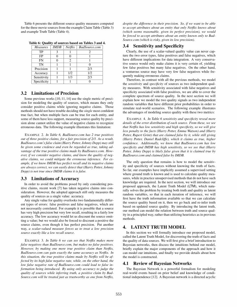
Table 6 presents the different source quality measures computedfor the three movie sources from the example Claim Table (Table 3)and example Truth Table (Table 4).

Table 6: Quality of sources based on Tables 3 and 4.Measures IMDB Netflix BadSource.com

TP 3 1 2FP 0 0 1FN 0 2 1TN 1 1 0

Precision 1 1 2/3Accuracy 1 1/2 1/2Sensitivity 1 1/3 2/3Specificity 1 1 0

3.2 Limitations of PrecisionSome previous works [10, 11, 14] use the single metric of preci-

sion for modeling the quality of sources, which means they onlyconsider positive claims while ignoring negative claims. Thosemethods should not have trouble deciding the single most confidenttrue fact, but when multiple facts can be true for each entity, andsome of them have less support, measuring source quality by preci-sion alone cannot utilize the value of negative claims to recognizeerroneous data. The following example illustrates this limitation:

EXAMPLE 2. In Table 6, BadSource.com has 2 true positivesout of three positive claims, for a fair precision of 2/3. As a result,BadSource.com’s false claim (Harry Potter, Johnny Depp) may stillbe given some credence and even be regarded as true, taking ad-vantage of the true positive claims made by BadSource.com. How-ever, if we consider negative claims, and know the quality of neg-ative claims, we could mitigate the erroneous inference. For ex-ample, if we know IMDB has perfect recall and its negative claimsare always correct, we can easily detect that (Harry Potter, JohnnyDepp) is not true since IMDB claims it is false.

3.3 Limitations of AccuracyIn order to avoid the problems posed by only considering pos-

itive claims, recent work [7] has taken negative claims into con-sideration. However, the adopted approach still only measures thequality of sources as a single value: accuracy.

Any single value for quality overlooks two fundamentally differ-ent types of errors: false positives and false negatives, which arenot necessarily correlated. For example it is possible that a sourcehas very high precision but very low recall, resulting in a fairly lowaccuracy. The low accuracy would let us discount the source omit-ting a value; but we would also be forced to discount a positive thesource claims, even though it has perfect precision. Put anotherway, a scalar-valued measure forces us to treat a low precisionsource exactly like a low recall source.

EXAMPLE 3. In Table 6 we can see that Netflix makes morefalse negatives than BadSource.com, but makes no false positives.However, by making one more true positive claim than Netflix,BadSource.com can gain exactly the same accuracy as Netflix. Inthis situation, the true positive claims made by Netflix will be af-fected by its high false negative rate, while, on the other hand, thelow false negative rate of BadSource.com could lead to false in-formation being introduced. By using only accuracy to judge thequality of sources while inferring truth, a positive claim by Bad-Source.com will be treated just as trustworthy as one from Netflix,

despite the difference in their precision. So, if we want to be ableto accept attributes about an entity that only Netflix knows about(which seems reasonable, given its perfect precision), we wouldbe forced to accept attributes about an entity known only to Bad-Source.com (which is risky, given its low precision).

3.4 Sensitivity and SpecificityClearly, the use of a scalar-valued quality value can never cap-

ture the two error types, false positives and false negatives, whichhave different implications for data integration. A very conserva-tive source would only make claims it is very certain of, yieldingfew false positives but many false negatives. On the other hand,a venturous source may have very few false negatives while fre-quently making erroneous claims.

Therefore, in contrast with all the previous methods, we modelthe sensitivity and specificity of sources as two independent qual-ity measures. With sensitivity associated with false negatives andspecificity associated with false positives, we are able to cover thecomplete spectrum of source quality. In the next section we willexplain how we model the two quality signals as two independentrandom variables that have different prior probabilities in order tosimulate real-world scenarios. The following example illustratesthe advantages of modeling source quality with these two metrics:

EXAMPLE 4. In Table 6 sensitivity and specificity reveal moredetails of the error distribution of each source. From these, we seethat Netflix has low sensitivity and high specificity, so we will giveless penalty to the facts (Harry Potter, Emma Watson) and (HarryPotter, Rupert Grint) that are claimed false by it, while still giving(Harry Potter, Daniel Radcliffe), which it claims as true, higherconfidence. Additionally, we know that BadSource.com has lowspecificity and IMDB has high sensitivity, so we see that (HarryPotter, Johny Depp) is likely false given that it is claimed true byBadSource.com and claimed false by IMDB.

The only question that remains is how to model the sensitiv-ity and specificity of sources without knowing the truth of facts.So far, our examples have implicitly assumed a supervised settingwhere ground truth is known and is used to calculate quality mea-sures, while in practice unsupervised methods that do not have suchknowledge are required. In the next section, we will introduce ourproposed approach, the Latent Truth Model (LTM), which natu-rally solves the problem by treating both truth and quality as latentrandom variables, so that in each iteration of inference, we willfirst have the truth information available so that we can calculatethe source quality based on it, then we go back and re-infer truthbased on updated source quality. By introducing the latent truth,our method can model the relation between truth and source qual-ity in a principled way, rather than utilizing heuristics as in previousmethods.

4. LATENT TRUTH MODELIn this section we will formally introduce our proposed model,

called the Latent Truth Model, for discovering the truth of facts andthe quality of data sources. We will first give a brief introduction toBayesian networks, then discuss the intuitions behind our model,briefly explain the major components of the approach and how itcan model our intuitions, and finally we provide details about howthe model is constructed.

4.1 Review of Bayesian NetworksThe Bayesian Network is a powerful formalism for modeling

real-world events based on prior belief and knowledge of condi-tional independence [12]. A Bayesian network is a directed acyclic

553

probabilistic graphical model in the Bayesian sense: each node rep-resents a random variable, which could be observed values, latent(unobserved) values, or unknown parameters. A directed edge fromnode a to b (a is then called the parent of b) models the conditionaldependence between a and b in the sense that the random variableassociated with a child node follows a probabilistic conditional dis-tribution that takes values depending on the parent nodes as param-eters.

Given the observed data and prior and conditional distributions,various inference algorithms can perform maximum a posteriori(MAP) estimation to assign latent variables and unknown parame-ters values that (approximately) maximize the posterior likelihoodsof those corresponding unobserved variables given the data.

Bayesian networks have been proven to be effective in numeroustasks such as information extraction, clustering, text mining, etc.In this work, our proposed Latent Truth Model is a new Bayesiannetwork for inferring truth and source quality for data integration.

4.2 Intuition Behind the Latent Truth ModelWe next describe the intuition behind modeling the quality of

sources, truth of facts and claim observations as random variables,before detailing the LTM graphical model in the next section.

4.2.1 Quality of SourcesAs discussed in the previous section, we need to model the qual-

ity of sources as two independent factors: specificity and sensi-tivity, and therefore in our model we create two separate randomvariables for each source, one associated with its specificity andthe other with its sensitivity.

Moreover, in practice we often have prior belief or assumptionswith regard to the data sources. For example, it is reasonable toassume that the majority of data coming from each source is noterroneous, i.e., the specificity of data sources should be reasonablyhigh. On the other hand, we could also assume missing data isfairly common, i.e., sensitivity may not be high for every source.It is also possible that we have certain prior knowledge about thequality of some specific data sources that we want to incorporateinto the model. In all these cases, the model should be able toallow us to plug in such prior belief. For this reason, in LTM wemodel source quality in the Bayesian tradition so that any availableassumptions or domain knowledge can be easily incorporated byspecifying prior distributions for the source quality variables. Inthe absence of such knowledge, we can simply use uniform priors.

4.2.2 Truth of FactsIn LTM we model the probability of (or belief in) each fact being

true as an unknown or latent random variable in the unit interval.In addition, we also introduce the actual truth label of each fact,which depends on the represented probability, as a latent Booleanrandom variable. By doing so, at any stage of the computation wecan clearly distinguish the two types of errors (false positives andfalse negatives) so that the specificity and sensitivity of sources canbe modeled in a natural and principled way.

In addition, if we have any prior belief about how likely all orcertain specific facts are true, our model can also support this infor-mation by setting prior distributions for the truth probability. Oth-erwise, we use a uniform prior.

4.2.3 Observation of ClaimsNow we need to model our actual observed data: claims from

different sources. Recall that each claim has three components:the fact it refers to, the source it comes from and the observation(True/False). Clearly, the observation of the claim depends on two

C

S

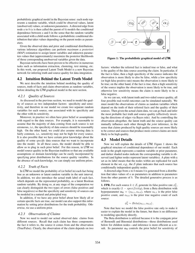
Figure 1: The probabilistic graphical model of LTM.

factors: whether the referred fact is indeed true or false, and whatis the quality of the data source asserting the claim. In particular, ifthe fact is false, then a high specificity of the source indicates theobservation is more likely to also be false, while a low specificity(or high false positive rate) means the observation is more likely tobe true; on the other hand, if the fact is true, then a high sensitivityof the source implies the observation is more likely to be true, andotherwise low sensitivity means the claim is more likely to be afalse negative.

As we can see, with latent truth and two-sided source quality, allfour possible real-world outcomes can be simulated naturally. Wemust model the observations of claims as random variables whichdepend on the truth of their referred facts and the quality of theirsources. Then given the actual claim data, we can go back and inferthe most probable fact truth and source quality (effectively invert-ing the directions of edges via Bayes rule). And by controlling theobservation altogether, the latent truth and the source quality canmutually influence each other through the joint inference, in thesense that claims produced by high quality sources are more likelyto be correct and sources that produce more correct claims are morelikely to be high quality.

4.3 Model DetailsNow we will explain the details of LTM. Figure 1 shows the

graphical structure of conditional dependence of our model. Eachnode in the graph represents a random variable or prior parameter,and darker shaded nodes indicate the corresponding variable is ob-served (and lighter nodes represent latent variables). A plate with aset as its label means that the nodes within are replicated for eachelement in the set, e.g., the S plate indicates that each source hasconditionally independent quality nodes.

A directed edge from a to bmeans b is generated from a distribu-tion that takes values of a as parameters in addition to parametersfrom the other parents of b. The detailed generative process is asfollows.1. FPR. For each source k ∈ S, generate its false positive rate φ0

k,which is exactly (1 − specificity), from a Beta distribution withhyperparameter α0 = (α0,1, α0,0), where α0,1 is the prior falsepositive count, and α0,0 is the prior true negative count of eachsource:

φ0k ∼ Beta(α0,1, α0,0) .

Note that here we model the false positive rate only to make iteasier to explain the model in the future, but there is no differenceto modeling specificity directly.

The Beta distribution is utilized because it is the conjugate priorof Bernoulli and Binomial distributions—those distributions usedbelow for children nodes—and inference is more efficient as a re-sult. Its parameter α0 controls the prior belief for sensitivity of

554

sources, and in practice, we set α0,0 significantly higher than α1,0

to plug in our assumptions that sources in general are good anddo not have high false positive rate, which is not only reasonablebut also important since otherwise the model could flip every truthwhile still achieving high likelihood thereby making incorrect in-ferences.2. Sensitivity. For each source k ∈ S, generate its sensitivity φ1

k

from a Beta distribution with hyperparameter α1 = (α1,1, α1,0),where α1,1 is the prior true positive count, and α1,0 is the falsenegative count of each source:

φ1k ∼ Beta(α1,1, α1,0) .

Similar toα0 above,α1 controls the prior distribution for sensitiv-ity of sources. Since in practice we observe that it is quite commonfor some sources to ignore true facts and therefore generate falsenegative claims, we will not specify a strong prior for α1 as we dofor α0, instead we can just use a uniform prior.3. Per fact. For each fact f ∈ F ,3(a). Prior truth probability. Generate prior truth probability θffrom a Beta distribution with hyperparameter β = (β1, β0), whereβ1 is the prior true count, and β0 is the prior false count of eachfact:

θf ∼ Beta(β1, β0) .

Here β determines the prior distribution of how likely each fact isto be true. In practice, if we do not have a strong belief, we can usea uniform prior meaning it is equally likely to be true or false andthe model can still effectively infer the truth from other factors inthe model.3(b). Truth label. Generate the truth label tf from a Bernoullidistribution with parameter θf :

tf ∼ Bernoulli(θf ) .

As a result, tf is a Boolean variable, and the prior probability thattf is true is exactly θf .3(c). Observation. For each claim c of fact f , i.e., c ∈ Cf , denoteits source as sc, which is an observed dummy index variable thatwe use to select the corresponding source quality. We generate theobservation of c from a Bernoulli distribution with parameter φ

tfsc ,

i.e., quality parameter of source sc depending on tf , the truth of f :

oc ∼ Bernoulli(φtfsc ) .

Specifically, if tf = 0, then oc is generated from a Bernoullidistribution with parameter φ0

sc , i.e., the false positive rate of sc,as:

oc ∼ Bernoulli(φ0sc) .

Then the resulting value of oc is Boolean. If it is true then theclaim is a false positive claim and its probability is exactly the falsepositive rate of sc.

If tf = 1, oc is generated from a Bernoulli distribution withparameter φ1

sc , i.e., the sensitivity of sc:

oc ∼ Bernoulli(φ1sc) .

Then in this case the probability that the Boolean variable oc is trueis exactly the sensitivity or true positive rate of sc as desired.

5. INFERENCE ALGORITHMSIn this section we discuss how to perform inference to estimate

the truth of facts and quality of sources from the model, given theobserved claim data.

5.1 Likelihood FunctionsAccording to the Latent Truth Model, the probability of each

claim c of fact f given the LTM parameters is:

p(oc|θf , φ0sc , φ

1sc) = p(oc|φ0

sc)(1− θf ) + p(oc|φ1sc)θf .

Then the complete likelihood of all observations, latent variablesand unknown parameters given the hyperparameters α0, α1, β is:

p(o, s, t,θ,φ0,φ1|α0,α1,β) =∏s∈S

p(φ0s|α0)p(φ

1s|α1)×

×∏f∈F

p(θf |β) ∑tf∈0,1

θtff (1− θf )1−tf

∏c∈Cf

p(oc|φtfsc )

.

(1)

5.2 Truth via Collapsed Gibbs SamplingGiven observed claim data, we must find assignments of latent

truth that maximize the joint probability, i.e., get the maximum aposterior (MAP) estimate for t:

t̂MAP = argmaxt

∫ ∫ ∫p(o, s, t,θ,φ0,φ1)dθdφ0dφ1 .

As we can see, a brute force inference method that searches thespace of all possible truth assignment t would be prohibitively in-efficient. So we need to develop a much faster inference algorithm.

Gibbs sampling is a Markov chain Monte Carlo (MCMC) algo-rithm that can estimate joint distributions that are not easy to di-rectly sample from. The MCMC process is to iteratively sampleeach variable from its conditional distribution given all the othervariables, so that the sequence of samples forms a Markov chain,the stationary distribution of which is just the exact joint distribu-tion we want to estimate.

Moreover, LTM utilizes the conjugacy of exponential familieswhen modeling the truth probability θ, source specificity φ0 andsensitivity φ1, so that they can be integrated out in the samplingprocess, i.e., we can just iteratively sample the truth of facts andavoid sampling these other quantities, which yields even greaterefficiency. Such a sampler is commonly referred to as a collapsedGibbs sampler.

Let t−f be the truth of all facts in F except f . We iterativelysample for each fact given the current truth labels of other facts:

p(tf = i|t−f ,o, s) ∝ βi∏c∈Cf

n−fsc,i,oc + αi,oc

n−fsc,i,1 + n−fsc,i,0 + αi,1 + αi,0

(2)

where

n−fsc,i,j = |{c′ ∈ C−f |sc′ = sc, tfc′ = i, oc′ = j}| ,

i.e., the number of sc’s claims whose observation is j, and referredfact is not f and its truth is i. These counts reflect the quality of scbased on claims of facts other than f , e.g., n−fsc,0,0 is the number oftrue negative claims of sc, n−fsc,0,1 is the false positive count, n−fsc,1,0is the false negative count, and n−fsc,1,1 is the true positive count.

The detailed derivation of Equation (2) can be found in Ap-pendix A. Intuitively, it can be interpreted as sampling the truthof each fact based on the prior for truth and the quality signals ofassociated sources estimated on other facts.

Algorithm 1 presents pseudo-code for implementing the collapsedGibbs sampling algorithm. We initialize by randomly assigningeach fact a truth value, and calculate the initial counts for eachsource. Then in each iteration, we re-sample each truth variable

555

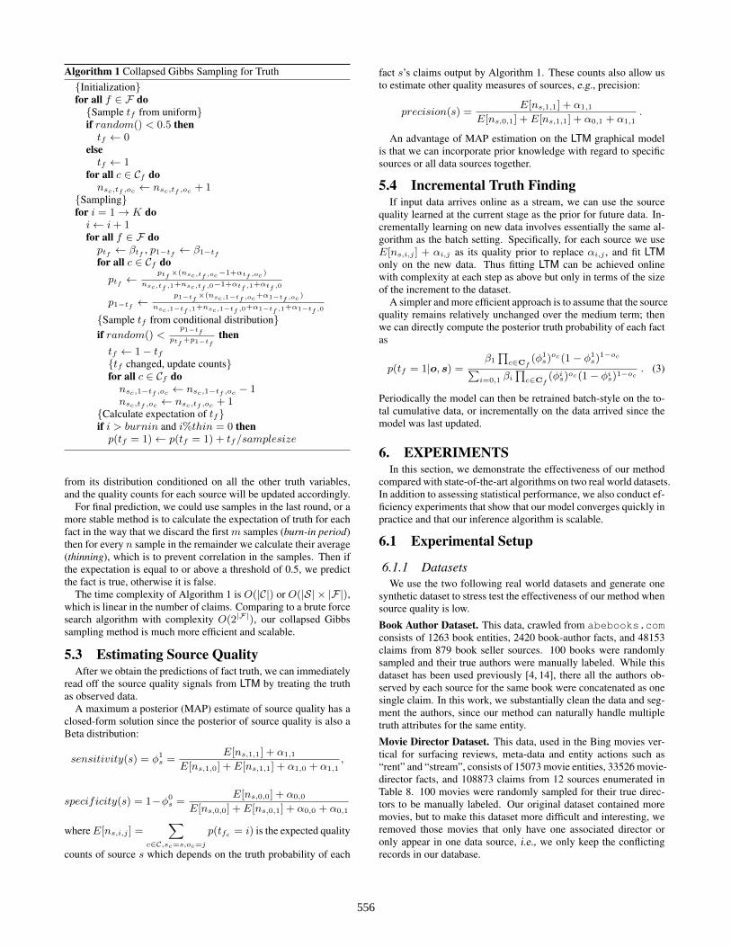
Algorithm 1 Collapsed Gibbs Sampling for Truth{Initialization}for all f ∈ F do{Sample tf from uniform}if random() < 0.5 thentf ← 0

elsetf ← 1

for all c ∈ Cf donsc,tf ,oc ← nsc,tf ,oc + 1

{Sampling}for i = 1→ K doi← i+ 1for all f ∈ F doptf ← βtf , p1−tf ← β1−tffor all c ∈ Cf doptf ←

ptf×(nsc,tf ,oc−1+αtf ,oc )

nsc,tf ,1+nsc,tf ,0−1+αtf ,1+αtf ,0

p1−tf ←p1−tf

×(nsc,1−tf ,oc+α1−tf ,oc )

nsc,1−tf ,1+nsc,1−tf ,0+α1−tf ,1+α1−tf ,0

{Sample tf from conditional distribution}if random() <

p1−tf

ptf +p1−tfthen

tf ← 1− tf{tf changed, update counts}for all c ∈ Cf donsc,1−tf ,oc ← nsc,1−tf ,oc − 1nsc,tf ,oc ← nsc,tf ,oc + 1

{Calculate expectation of tf}if i > burnin and i%thin = 0 thenp(tf = 1)← p(tf = 1) + tf/samplesize

from its distribution conditioned on all the other truth variables,and the quality counts for each source will be updated accordingly.

For final prediction, we could use samples in the last round, or amore stable method is to calculate the expectation of truth for eachfact in the way that we discard the first m samples (burn-in period)then for every n sample in the remainder we calculate their average(thinning), which is to prevent correlation in the samples. Then ifthe expectation is equal to or above a threshold of 0.5, we predictthe fact is true, otherwise it is false.

The time complexity of Algorithm 1 is O(|C|) or O(|S| × |F|),which is linear in the number of claims. Comparing to a brute forcesearch algorithm with complexity O(2|F|), our collapsed Gibbssampling method is much more efficient and scalable.

5.3 Estimating Source QualityAfter we obtain the predictions of fact truth, we can immediately

read off the source quality signals from LTM by treating the truthas observed data.

A maximum a posterior (MAP) estimate of source quality has aclosed-form solution since the posterior of source quality is also aBeta distribution:

sensitivity(s) = φ1s =

E[ns,1,1] + α1,1

E[ns,1,0] + E[ns,1,1] + α1,0 + α1,1,

specificity(s) = 1−φ0s =

E[ns,0,0] + α0,0

E[ns,0,0] + E[ns,0,1] + α0,0 + α0,1

whereE[ns,i,j ] =∑

c∈C,sc=s,oc=j

p(tfc = i) is the expected quality

counts of source s which depends on the truth probability of each

fact s’s claims output by Algorithm 1. These counts also allow usto estimate other quality measures of sources, e.g., precision:

precision(s) =E[ns,1,1] + α1,1

E[ns,0,1] + E[ns,1,1] + α0,1 + α1,1.

An advantage of MAP estimation on the LTM graphical modelis that we can incorporate prior knowledge with regard to specificsources or all data sources together.

5.4 Incremental Truth FindingIf input data arrives online as a stream, we can use the source

quality learned at the current stage as the prior for future data. In-crementally learning on new data involves essentially the same al-gorithm as the batch setting. Specifically, for each source we useE[ns,i,j ] + αi,j as its quality prior to replace αi,j , and fit LTMonly on the new data. Thus fitting LTM can be achieved onlinewith complexity at each step as above but only in terms of the sizeof the increment to the dataset.

A simpler and more efficient approach is to assume that the sourcequality remains relatively unchanged over the medium term; thenwe can directly compute the posterior truth probability of each factas

p(tf = 1|o, s) =β1

∏c∈Cf

(φ1s)oc(1− φ1

s)1−oc∑

i=0,1 βi∏c∈Cf

(φis)oc(1− φis)1−oc. (3)

Periodically the model can then be retrained batch-style on the to-tal cumulative data, or incrementally on the data arrived since themodel was last updated.

6. EXPERIMENTSIn this section, we demonstrate the effectiveness of our method

compared with state-of-the-art algorithms on two real world datasets.In addition to assessing statistical performance, we also conduct ef-ficiency experiments that show that our model converges quickly inpractice and that our inference algorithm is scalable.

6.1 Experimental Setup

6.1.1 DatasetsWe use the two following real world datasets and generate one

synthetic dataset to stress test the effectiveness of our method whensource quality is low.

Book Author Dataset. This data, crawled from abebooks.comconsists of 1263 book entities, 2420 book-author facts, and 48153claims from 879 book seller sources. 100 books were randomlysampled and their true authors were manually labeled. While thisdataset has been used previously [4, 14], there all the authors ob-served by each source for the same book were concatenated as onesingle claim. In this work, we substantially clean the data and seg-ment the authors, since our method can naturally handle multipletruth attributes for the same entity.

Movie Director Dataset. This data, used in the Bing movies ver-tical for surfacing reviews, meta-data and entity actions such as“rent” and “stream”, consists of 15073 movie entities, 33526 movie-director facts, and 108873 claims from 12 sources enumerated inTable 8. 100 movies were randomly sampled for their true direc-tors to be manually labeled. Our original dataset contained moremovies, but to make this dataset more difficult and interesting, weremoved those movies that only have one associated director oronly appear in one data source, i.e., we only keep the conflictingrecords in our database.

556

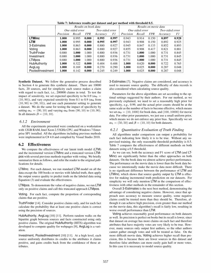
Table 7: Inference results per dataset and per method with threshold 0.5.Results on book data Results on movie data

One-sided error Two-sided error One-sided error Two-sided errorPrecision Recall FPR Accuracy F1 Precision Recall FPR Accuracy F1

LTMinc 1.000 0.995 0.000 0.995 0.997 0.943 0.914 0.150 0.897 0.928LTM 1.000 0.995 0.000 0.995 0.997 0.943 0.908 0.150 0.892 0.9253-Estimates 1.000 0.863 0.000 0.880 0.927 0.945 0.847 0.133 0.852 0.893Voting 1.000 0.863 0.000 0.880 0.927 0.855 0.908 0.417 0.821 0.881TruthFinder 0.880 1.000 1.000 0.880 0.936 0.731 1.000 1.000 0.731 0.845Investment 0.880 1.000 1.000 0.880 0.936 0.731 1.000 1.000 0.731 0.845LTMpos 0.880 1.000 1.000 0.880 0.936 0.731 1.000 1.000 0.731 0.845HubAuthority 1.000 0.322 0.000 0.404 0.488 1.000 0.620 0.000 0.722 0.765AvgLog 1.000 0.169 0.000 0.270 0.290 1.000 0.025 0.000 0.287 0.048PooledInvestment 1.000 0.142 0.000 0.245 0.249 1.000 0.025 0.000 0.287 0.048

Synthetic Dataset. We follow the generative process describedin Section 4 to generate this synthetic dataset. There are 10000facts, 20 sources, and for simplicity each source makes a claimwith regard to each fact, i.e., 200000 claims in total. To test theimpact of sensitivity, we set expected specificity to be 0.9 (α0 =(10, 90)), and vary expected sensitivity from 0.1 to 0.9 (α0 from(10, 90) to (90, 10)), and use each parameter setting to generatea dataset. We do the same for testing the impact of specificity bysetting α1 = (90, 10) and varying α0 from (90, 10) to (10, 90).In all datasets β = (10, 10).

6.1.2 EnvironmentAll the experiments presented were conducted on a workstation

with 12GB RAM, Intel Xeon 2.53GHz CPU, and Windows 7 Enter-prise SP1 installed. All the algorithms including previous methodswere implemented in C# 4.0 and complied by Visual Studio 2010.

6.2 EffectivenessWe compare the effectiveness of our latent truth model (LTM)

and the incremental version LTMinc and a truncated version LTM-pos with several previous methods together with voting. We brieflysummarize them as follows, and refer the reader to the original pub-lications for details.

LTMinc. For each dataset, we run standard LTM model on all thedata except the 100 books or movies with labeled truth, then applythe output source quality to predict truth on the labeled data usingEquation (3) and evaluate the effectiveness.

LTMpos. To demonstrate the value of negative claims, we run LTMonly on positive claims and call this truncated approach LTMpos.

Voting. For each fact, compute the proportion of correspondingclaims that are positive.

TruthFinder [14]. Consider positive claims only, and for each factcalculate the probability that at least one positive claim is correctusing the precision of sources.

HubAuthority, AvgLog [10] [11]. Perform random walks on thebipartite graph between sources and facts constructed using onlypositive claims. The original HubAuthority (HITS) algorithm wasdeveloped to compute quality for webpages [9], AvgLog is a vari-ation.

Investment, PooledInvestment [10] [11]. At a high level, eachsource uniformly distributes its credits to the attributes it claimspositive, and gains credits back from the confidence of those at-tributes.

3-Estimates [7]. Negative claims are considered, and accuracy isused to measure source quality. The difficulty of data records isalso considered when calculating source quality.

Parameters for the above algorithms are set according to the op-timal settings suggested by their authors. For our method, as wepreviously explained, we need to set a reasonably high prior forspecificity, e.g., 0.99, and the actual prior counts should be at thesame scale as the number of facts to become effective, which meanswe setα0 = (10, 1000) for book data, and (100, 10000) for moviedata. For other prior parameters, we just use a small uniform prior,which means we do not enforce any prior bias. Specifically we setα1 = (50, 50) and β = (10, 10) for both datasets.

6.2.1 Quantitative Evaluation of Truth FindingAll algorithms under comparison can output a probability for

each fact indicating how likely it is to be true. Without any su-pervised training, the only reasonable threshold probability is 0.5.Table 7 compares the effectiveness of different methods on bothdatasets using a 0.5 threshold.

As we can see, both the accuracy and F1 score of LTM (and LT-Minc) are significantly better than the other approaches on bothdatasets. On the book data we almost achieve perfect performance.The performance on the movie data is lower than the book data be-cause we intentionally make the movie data more difficult. Thereis no significant difference between the performance of LTM andLTMinc, which shows that source quality output by LTM is effec-tive for making incremental truth prediction on our datasets. Forsimplicity we will only mention LTM in the comparison of effec-tiveness with other methods in the remainder of this section.

Overall 3-Estimates is the next best method, demonstrating theadvantage of considering negative claims. However, since that ap-proach uses accuracy to measure source quality, some negativeclaims could be trusted more than they should be. Therefore, al-though it can achieve high precision, even greater than our methodon the movie data, this algorithm’s recall is fairly low, resulting inworse overall performance than LTM.

Voting achieves reasonably good performance on both datasetsas well. Its precision is perfect on books but its recall is lower, sincethat dataset on average has more claims on each fact and thereforeattributes that have majority votes are very likely to be true. How-ever, many sources only output first authors, so the other authorscannot gather enough votes and will be treated as false. On themore difficult movie data, Voting achieves higher recall than pre-cision, this is because there are fewer sources in this dataset andtherefore false attributes can more easily gain half or more votes.In this case it is necessary to model source quality.

557

0.0 0.2 0.4 0.6 0.8 1.0

0.0

0.2

0.4

0.6

0.8

1.0

Inferring True Book Authors

Threshold probability

Accura

cy

LTM

LTMinc

LTMpos

TruFinder

AvgLog

HubAuth

Invest

PInvest

3Est

Voting

0.0 0.2 0.4 0.6 0.8 1.0

0.0

0.2

0.4

0.6

0.8

1.0

Inferring True Movie Directors

Threshold probability

Accura

cy

LTM

LTMinc

LTMpos

TruFinder

AvgLog

HubAuth

Invest

PInvest

3Est

Voting

Figure 2: Accuracy vs. thresholds on the book data and the movie data.

Movies

Books

Truth Finding Performance Summary

Method

Are

a U

nder

Curv

e

0.0

0.2

0.4

0.6

0.8

1.0

LTM

inc

LTM

3Est

Votin

g

Hub

Auth

PInve

st

AvgLo

g

TruF

inde

r

LTM

pos

Inve

st

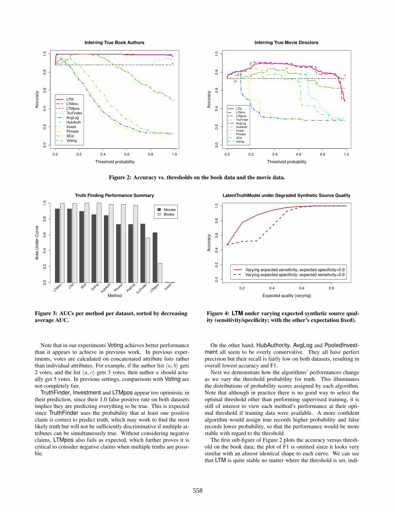
Figure 3: AUCs per method per dataset, sorted by decreasingaverage AUC.

0.2 0.4 0.6 0.8

0.0

0.2

0.4

0.6

0.8

1.0

LatentTruthModel under Degraded Synthetic Source Quality

Expected quality (varying)

Accura

cy

Varying expected sensitivity; expected specificity=0.9Varying expected specificity; expected sensitivity=0.9

Figure 4: LTM under varying expected synthetic source qual-ity (sensitivity/specificity; with the other’s expectation fixed).

Note that in our experiments Voting achieves better performancethan it appears to achieve in previous work. In previous exper-iments, votes are calculated on concatenated attribute lists ratherthan individual attributes. For example, if the author list 〈a, b〉 gets2 votes, and the list 〈a, c〉 gets 3 votes, then author a should actu-ally get 5 votes. In previous settings, comparisons with Voting arenot completely fair.

TruthFinder, Investment and LTMpos appear too optimistic intheir prediction, since their 1.0 false positive rate on both datasetsimplies they are predicting everything to be true. This is expectedsince TruthFinder uses the probability that at least one positiveclaim is correct to predict truth, which may work to find the mostlikely truth but will not be sufficiently discriminative if multiple at-tributes can be simultaneously true. Without considering negativeclaims, LTMpos also fails as expected, which further proves it iscritical to consider negative claims when multiple truths are possi-ble.

On the other hand, HubAuthority, AvgLog and PooledInvest-ment all seem to be overly conservative. They all have perfectprecision but their recall is fairly low on both datasets, resulting inoverall lowest accuracy and F1.

Next we demonstrate how the algorithms’ performances changeas we vary the threshold probability for truth. This illuminatesthe distributions of probability scores assigned by each algorithm.Note that although in practice there is no good way to select theoptimal threshold other than performing supervised training, it isstill of interest to view each method’s performance at their opti-mal threshold if training data were available. A more confidentalgorithm would assign true records higher probability and falserecords lower probability, so that the performance would be morestable with regard to the threshold.

The first sub-figure of Figure 2 plots the accuracy versus thresh-old on the book data; the plot of F1 is omitted since it looks verysimilar with an almost identical shape to each curve. We can seethat LTM is quite stable no matter where the threshold is set, indi-

558

cating our method can discriminate between true and false betterthan other methods. Voting and 3-Estimates are rather conserva-tive, since their optimal threshold is around 0.2, where their per-formance is even on par with our method. However, in practice itis difficult to find such an optimal threshold. Their performancedrops very fast when the threshold increases above 0.5, since morefalse negatives are produced. The optimal threshold for HubAu-thority, AvgLog, and PooledInvestment are even lower and theirperformance drops even faster when the threshold increases, indi-cating they are more conservative by assigning data lower proba-bility than deserved. On the other hand, TruthFinder, Investmentand LTMpos are overly optimistic. We can see the optimal thresh-old for TruthFinder is around 0.95, meaning its output scores aretoo high. Investment and LTMpos consistently think everythingis true even at a higher threshold.

The second sub-figure of Figure 2 is the analogous plot on themovie data, which is more difficult than the book data. AlthoughLTM is not as stable as on the book data, we can see that it is stillconsistently better than all the other methods in the range from 0.2to 0.9, clearly indicating our method is more discriminative andstable. 3-Estimates achieves its optimal threshold around 0.5, andVoting has its peak performance around 0.4, which is still worsethan LTM, indicating source quality becomes more important whenconflicting records are more common. For other methods, Pooled-Investment and AvgLog are still rather conservative, while Invest-ment and LTMpos continue to be overly optimistic. However, itseems TruthFinder and HubAuthority enjoy improvements on themovie data.

Next in Figure 3 we show the area under the ROC curve (AUC)metric of each algorithm on both datasets, which summarizes theperformance of each algorithm in ROC space and quantitativelyevaluates capability of correctly ranking random facts by score. Wecan see several methods can achieve AUC close to the ideal of 1 onthe book data, indicating that the book data would be fairly easygiven training data. On the movie data, however, LTM shows clearadvantage over 3-Estimates, Voting and the other methods. Over-all on both datasets our method is the superior one.

Last but not least, we would like to understand LTM’s behaviorwhen source quality degrades. Figure 4 shows the accuracy of LTMon the synthetic data when the expected specificity or sensitivity ofall sources is fixed while the other measure varies between 0.1 and0.9. We can see the accuracy stays close to 1 until the source qualitystarts to drop below 0.6, and it decreases much faster with regard tospecificity than sensitivity. This shows LTM is more tolerant of lowsensitivity, which proves to be effective in practice and is an ex-pected behavior since the chosen priors incorporate our belief thatspecificity of sources is usually high but sensitivity is not. Whenspecificity is around 0.3 (respectively sensitivity is around 0.1), theaccuracy drops to around 0.5 which means the prediction is nearlyrandom.

6.2.2 Case Study of Source Quality PredictionHaving evaluated the performance of our model on truth find-

ing, we may now explore whether the source quality predicted byour method is reasonable, bearing in mind that no ground truth isavailable with which to quantitatively validate quality. Indeed thisexercise should serve as a concrete example of what to expect whenreading off source quality (cf. Section 5.3).

Table 8 shows a MAP estimate of the sensitivity and specificityof sources from our model fit to the movie data, sorted by sen-sitivity. This table verifies some of our observations on the moviesources: IMDB tends to output rather complete records, while LTMassigns IMDB correspondingly high sensitivity. Note that we can

Table 8: Source quality on the movie data.Source Sensitivity Specificityimdb 0.911622836 0.898838631netflix 0.894019034 0.934833904

movietickets 0.862889367 0.978844687commonsense 0.809752315 0.982347827cinemasource 0.794184357 0.985847745

amg 0.776583683 0.690600694yahoomovie 0.760589896 0.897654374msnmovie 0.749192861 0.987870636

zune 0.744272491 0.973922421metacritic 0.678661638 0.987957893

flixster 0.584223615 0.911078627fandango 0.499623726 0.989836274

also observe in this table that sensitivity and specificity do not nec-essarily correlate. Some sources can do well or poorly on bothmetrics, and it is also common for more conservative sources toachieve lower sensitivity but higher specificity (Fandango), whilemore aggressive sources to get higher sensitivity but lower speci-ficity (IMDB). This further justifies the intuition that we ought tomodel the quality of sources as two independent factors.

6.3 EfficiencyWe now study the scalability of LTM and LTMinc.

6.3.1 Convergence RateSince our inference algorithm is an iterative method, we now ex-

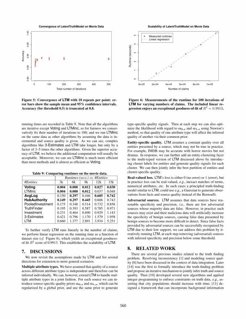
plore how many iterations it requires in practice to reach reasonableaccuracy. To evaluate convergence rate, in the same run of the al-gorithm, we make 7 sequential predictions using the samples in thefirst 7, 10, 20, 50, 100, 200, 500 iterations, with burn in iterations2, 2, 5, 10, 20, 50, 100, and sample gap 0, 0, 0, 1, 4, 4, 9 re-spectively. We repeat 10 times to account for randomization due tosampling, and calculate the average accuracy and 95% confidenceintervals on the 10 runs for each of the 7 predictions, as shown inFigure 5. One can see that accuracy quickly reaches 0.85 even afteronly 7 iterations, although in the first few iterations mean accuracyincreases and variation decreases, implying that the algorithm hasyet to converge. After only 50 iterations, the algorithm achievesoptimal accuracy and extremely low variation, with additional iter-ations not improving performance further. Thus we conclude thatLTM inference converges quickly in practice.

6.3.2 RuntimeWe now compare the running time of LTM and LTMinc with

previous methods. Although it is easy to see that our algorithmsand previous methods all have linear complexity in the number ofclaims in the data, we expected from the outset that our more prin-cipled approach LTM would take more time since it is more com-plex and requires costly procedures such as generating a randomnumber for each fact in each iteration. However, we can clearly seeits effective, incremental version LTMinc is much more efficientwithout needing any iteration. In particular we recommend that inefficiency-critical situations, standard LTM be infrequently run of-fline to update source quality and LTMinc be deployed for onlineprediction.

We created 4 smaller datasets by randomly sampling 3k, 6k, 9k,and 12k movies from the entire 15k movie dataset and by pullingall facts and claims associated with the sampled movies. We thenran each algorithm 10 times on the 5 datasets, for which the average

559

0 100 200 300 400 500

0.8

00

.85

0.9

00

.95

1.0

0Convergence of LatentTruthModel on Movie Data

Total number of iterations

Accura

cy

Figure 5: Convergence of LTM with 10 repeats per point: er-ror bars show the sample mean and 95% confidence intervals.Accuracy (for threshold 0.5) is truncated at 0.8.

0e+00 2e+04 4e+04 6e+04 8e+04 1e+05

01

23

45

Scalability of LatentTruthModel on Movie Data

Number of claims

Runtim

e (

seconds)

Measured runtimesLinear regression

Figure 6: Measurements of the runtime for 100 iterations ofLTM for varying numbers of claims. The included linear re-gression enjoys an exceptional goodness-of-fit of R2 = 0.9913.

running times are recorded in Table 9. Note that all the algorithmsare iterative except Voting and LTMinc, so for fairness we conser-vatively fix their number of iterations to 100; and we run LTMincon the same data as other algorithms by assuming the data is in-cremental and source quality is given. As we can see, complexalgorithms like 3-Estimates and LTM take longer, but only by afactor of 3–5 times the other algorithms. Given the superior accu-racy of LTM, we believe the additional computation will usually beacceptable. Moreover, we can see LTMinc is much more efficientthan most methods and is almost as efficient as Voting.

Table 9: Comparing runtimes on the movie data.Runtimes (secs.) vs. #Entities

#Entities 3k 6k 9k 12k 15kVoting 0.004 0.008 0.012 0.027 0.030LTMinc 0.004 0.008 0.012 0.037 0.048AvgLog 0.150 0.297 0.446 0.605 0.742HubAuthority 0.149 0.297 0.445 0.606 0.743PooledInvestment 0.175 0.348 0.514 0.732 0.856TruthFinder 0.195 0.393 0.587 0.785 0.971Investment 0.231 0.464 0.690 0.929 1.1433-Estimates 0.421 0.796 1.170 1.579 1.958LTM 0.660 1.377 2.891 3.934 5.251

To further verify LTM runs linearly in the number of claims,we perform linear regression on the running time as a function ofdataset size (cf. Figure 6), which yields an exceptional goodness-of-fit R2 score of 0.9913. This establishes the scalability of LTM.

7. DISCUSSIONSWe now revisit the assumptions made by LTM and list several

directions for extension to more general scenarios.Multiple attribute types. We have assumed that quality of a sourceacross different attribute types is independent and therefore can beinferred individually. We can, however, extend LTM to handle mul-tiple attribute types in a joint fashion. For each source we can in-troduce source-specific quality priorsα0,s andα1,s, which can beregularized by a global prior, and use the same prior to generate

type-specific quality signals. Then at each step we can also opti-mize the likelihood with regard to α0,s and α1,s using Newton’smethod, so that quality of one attribute type will affect the inferredquality of another via their common prior.

Entity-specific quality. LTM assumes a constant quality over allentities presented by a source, which may not be true in practice.For example, IMDB may be accurate with horror movies but notdramas. In response, we can further add an entity-clustering layerto the multi-typed version of LTM discussed above by introduc-ing cluster labels for entities and generate quality signals for eachcluster. We can then jointly infer the best partition of entities andcluster-specific quality.

Real-valued loss. LTM’s loss is either 0 (no error) or 1 (error), butin practice loss can be real-valued, e.g., inexact matches of terms,numerical attributes, etc. In such cases a principled truth-findingmodel similar to LTM, could use e.g., a Gaussian to generate obser-vations from facts and source quality instead of the Bernoulli.

Adversarial sources. LTM assumes that data sources have rea-sonable specificity and precision, i.e., there are few adversarialsources whose majority data are false. However, in practice suchsources may exist and their malicious data will artificially increasethe specificity of benign sources, causing false data presented bybenign sources to become more difficult to detect. Since false factsprovided by adversarial sources can be successfully recognized byLTM due to their low support, we can address this problem by it-eratively running LTM, at each step removing (adversarial) sourceswith inferred specificity and precision below some threshold.

8. RELATED WORKThere are several previous studies related to the truth finding

problem. Resolving inconsistency [1] and modeling source qual-ity [6] have been discussed in the context of data integration. Later[14] was the first to formally introduce the truth-finding problemand propose an iterative mechanism to jointly infer truth and sourcequality. Then [10] developed several new algorithms and appliedinteger programming to enforce constraints on truth data, e.g., as-serting that city populations should increase with time; [11] de-signed a framework that can incorporate background information

560

such as how confidently records are extracted from sources; and [7]observed that the difficulty of merging data records should be con-sidered in modeling source quality, in the sense that sources wouldnot gain too much credit from records that are fairly easy to inte-grate. [13] proposed an EM algorithm for truth finding in sensornetworks, but the nature of claims and sensor quality in their set-ting is rather different than here. In this paper we implement mostof the previous algorithms except those models for handling infor-mation not available in our datasets, e.g., constraints on truths; andwe show that our proposed method outperforms the previous ap-proaches.

Past work also focuses on other aspects, or different data types,in data integration. The copying relationship between sources wasstudied in [3–5]. By detecting the copying relationship, the sup-port for erroneous data can be discounted and accuracy for truthfinding can be improved. [3] also showed it is beneficial to con-sider multiple attributes together rather than independently. [15]explored semi-supervised truth finding by utilizing the similaritybetween data records. [2] modeled source quality as relevance todesired queries in a deep web source selection setting. [8] focusedon finding truth from several knowledge bases.

9. CONCLUSIONSIn this paper, we propose a probabilistic graphical model called

the Latent Truth Model to solve the truth finding problem in data in-tegration. We observe that in practice there are two types of errors,false positive and false negative, which do not necessarily correlate,especially when multiple facts can be true for the same entities. Byintroducing the truth as a latent variable, our Bayesian approachcan model the generative error process and two-sided source qual-ity in a principled fashion, and can naturally support multiple truthsas a result. Experiments on two real world datasets demonstrate theclear advantage of our method over the state-of-the-art truth find-ing methods. A case-study of source quality predicted by our modelalso verifies our intuition that two aspects of source quality shouldbe considered. An efficient inference algorithm based on collapsedGibbs sampling is developed, which is shown through experimentsto converge quickly and cost linear time with regard to data size.Additionally, our method can naturally incorporate various priorknowledge about the distribution of truth or quality of sources, andit can be employed in an online streaming setting for incrementaltruth finding, which we prove to be much more efficient and as ef-fective as batch inference. We also list several future directions toimprove LTM for handling more general scenarios.

10. ACKNOWLEDGEMENTSWe thank Ashok Chandra, Duo Zhang, Sahand Negahban and

three anonymous reviewers for their valuable comments. The workwas supported in part by the U.S. Army Research Laboratory underCooperative Agreement No. W911NF-09-2-0053 (NS-CTA).

11. REFERENCES[1] M. Arenas, L. E. Bertossi, and J. Chomicki. Consistent query

answers in inconsistent databases. In PODS, pages 68–79, 1999.[2] R. Balakrishnan and S. Kambhampati. SourceRank: relevance and

trust assessment for deep web sources based on inter-sourceagreement. In WWW, pages 227–236, 2011.

[3] L. Blanco, V. Crescenzi, P. Merialdo, and P. Papotti. Probabilisticmodels to reconcile complex data from inaccurate data sources. InCAiSE, pages 83–97, 2010.

[4] X. L. Dong, L. Berti-Equille, and D. Srivastava. Integratingconflicting data: The role of source dependence. PVLDB,2(1):550–561, 2009.

[5] X. L. Dong, L. Berti-Equille, and D. Srivastava. Truth discovery andcopying detection in a dynamic world. PVLDB, 2(1):562–573, 2009.

[6] D. Florescu, D. Koller, and A. Y. Levy. Using probabilisticinformation in data integration. In VLDB, pages 216–225, 1997.

[7] A. Galland, S. Abiteboul, A. Marian, and P. Senellart. Corroboratinginformation from disagreeing views. In WSDM, pages 131–140,2010.

[8] G. Kasneci, J. V. Gael, D. H. Stern, and T. Graepel. CoBayes:Bayesian knowledge corroboration with assessors of unknown areasof expertise. In WSDM, pages 465–474, 2011.

[9] J. M. Kleinberg. Authoritative sources in a hyperlinked environment.J. ACM, 46(5):604–632, 1999.

[10] J. Pasternack and D. Roth. Knowing what to believe (when youalready know something). In COLING, pages 877–885, 2010.

[11] J. Pasternack and D. Roth. Making better informed trust decisionswith generalized fact-finding. In IJCAI, pages 2324–2329, 2011.

[12] S. Russell and P. Norvig. Artificial Intelligence: A Modern Approach.Prentice Hall, 3rd edition, 2009.

[13] D. Wang, T. Abdelzaher, L. Kaplan, and C. Aggarwal. Onquantifying the accuracy of maximum likelihood estimation ofparticipant reliability in social sensing. In DMSN, pages 7–12, 2011.

[14] X. Yin, J. Han, and P. S. Yu. Truth discovery with multiple conflictinginformation providers on the web. In KDD, pages 1048–1052, 2007.

[15] X. Yin and W. Tan. Semi-supervised truth discovery. In WWW, pages217–226, 2011.

APPENDIXA. DETAILS OF INFERENCE

We can apply Bayes rule to rewrite the conditional distributionof tf given t−f and the observed data as follows:

p(tf = i|t−f ,o, s)

∝ p(tf = i|t−f )∏c∈Cf

p(oc, sc|tf = i,o−f , s−f ) . (4)

We first rewrite the first term in Equation (4):

p(tf = i|t−f ) =∫p(tf = i|θf )p(θf |t−f )dθf

=1

B(β1, β0)

∫θβ1+i−1f (1− θf )β0+(1−i)−1dθf

=B(β1 + i, β0 + (1− i))

B(β1, β0)=

βiβ1 + β0

∝ βi .

For the remaining terms in Equation (4), we have:

p(oc, sc|tf = i,o−f , s−f )

∝∫p(oc|φisc)p(φ

isc |o−f , s−f )dφ

isc

∝∫p(oc|φisc)p(φ

isc)

∏c′ /∈Cf ,sc′=sc

p(oc′ |φisc)dφisc

∝∫(φisc)

oc+n−fsc,i,1

+αi,1−1(1− φisc)(1−oc)+n−f

sc,i,0+αi,0−1dφisc

B(n−fsc,i,1 + αi,1, n−fsc,i,0

+ αi,0)

=n−fsc,i,oc + αi,oc

n−fsc,i,1 + n−fsc,i,0 + αi,1 + αi,0.

Now we can incorporate the above two equations into Equation (4)to yield Equation (2).

561