a bayesian hierarchical model for prediction of latent
TRANSCRIPT
A Bayesian hierarchical model for prediction of
latent health states from multiple data sources
with application to active surveillance of
prostate cancer
R. Yates Coleya∗, Aaron J. Fishera, Mufaddal Mamawalab
H. Ballentine Carterb, Kenneth J. Pientab, and Scott L. Zegera
aDepartment of Biostatistics, Johns Hopkins Bloomberg School of Public Health
bJames Buchanan Brady Urological Institute, Johns Hopkins Medical Institutions
June 3, 2016
∗This research was supported by the Patrick C. Walsh Prostate Cancer Research Fund and a Patient-Centered
Outcomes Research Institute (PCORI) Award (ME-1408-20318). The statements presented in this article are
solely the responsibility of the authors and do not necessarily represent the views of the Patient-Centered Out-
comes Research Institute (PCORI), its Board of Governors or Methodology Committee. The authors gratefully
acknowledge Ruth Etzioni, Tom Louis, and Gary Rosner for their helpful comments.
1
arX
iv:1
508.
0751
1v4
[st
at.M
E]
1 J
un 2
016
1 Introduction
Medicine is in a period of transition. An ever-increasing amount of information is available on
patients ranging from genetic and epigenetic profiles enabled by next-generation sequencing to
moment-to-moment data collected by physical activity monitors. With this wealth of information
comes the opportunity to provide more targeted healthcare including, for example, prediction
of pre-clinical atherosclerosis (McGeachie et al., 2009), individualized cancer screening (Saini,
van Hees, and Vijan, 2014), sub-typing of scleroderma (Schulam, Wigley, and Saria, 2015), and
personalized cancer treatment (Hayden, 2009). In order to fully realize the promise of patient-
focused medicine, principled statistical methods are needed that integrate data from a variety
of sources in order to provide physicians and patients with relevant syntheses to inform their
decision-making. These methods must also accommodate limitations common to data generated
in an observational setting including measurement error and informative missing data patterns.
An excellent example of this challenge is low-risk prostate cancer diagnosis. Tumor lethality is
an aspect of an individual’s health state that is not directly observable but is manifest in multiple
types of measurements including biomarkers, histology of biopsied tissue, genetic markers, and
family history of the disease. Individualized predictions of the latent disease state are critical
to guide treatment decisions. If the tumor is potentially lethal, immediate treatment (including
surgery or radiation) can be life-saving. Yet, some tumors are indolent and not life-threatening.
In this case, treatment is not recommended due to the risk of lasting side effects including urinary
incontinence and erectile dysfunction (Chou et al., 2011).
Active surveillance (AS) offers an alternative to early treatment for individuals with lower risk
disease (Dall’Era et al., 2012). Though AS regimes vary, the approach generally entails regular
biopsies (e.g., annually) with intervention recommended upon detection of higher risk histological
features, as determined by the Gleason grading system (Gleason, 1992). Biopsies with a Gleason
score of 6 (the minimum for prostate cancer diagnosis) indicate low risk disease while a subsequent
Gleason score of 7 or above is considered “grade reclassification” (Tosoian et al., 2015); treatment
is recommended once grade reclassification is observed. Prostate-specific antigen (PSA), a blood
serum biomarker of inflammation in the prostate, is also routinely measured and may be used as
the basis for a biopsy recommendation.
2
The success of AS programs depends on clinicians’ ability to identify tumors with metastatic
potential with sufficient time for curative intervention to be effective. Yet, biopsies used to
characterize tumors typically sample less than one percent of the prostate tissue and so have
imperfect sensitivity and specificity (Epstein et al., 2012). Existing decision support tools that
predict biopsy outcomes for AS patients (including, most recently, Ankerst et al. (2015)) provide
patients and physicians with valuable information to guide decisions about biopsy timing and
frequency but are insufficient to directly address patients’ primary concerns about their tumors’
lethality. Patients and clinicians need predictions of the pathological make-up of the entire
prostate to guide their decision-making.
With this application in mind, we have developed a Bayesian hierarchical model that enables
prediction of an individual’s underlying disease state via joint modeling of repeated PSA mea-
surements and biopsies. Specifically, we predict a binary cancer state– indolent or aggressive–
with the latter defined as a “true” Gleason score of 7 or higher. Predictions are informed by a sub-
set of patients for whom the true state is observed– patients who, either before or after biopsy
grade reclassification, chose to undergo prostatectomy and have post-surgery, entire-prostate
Gleason score determinations. In this sense, cancer state operates as a partially-latent class in
the proposed model (Wu et al., 2015).
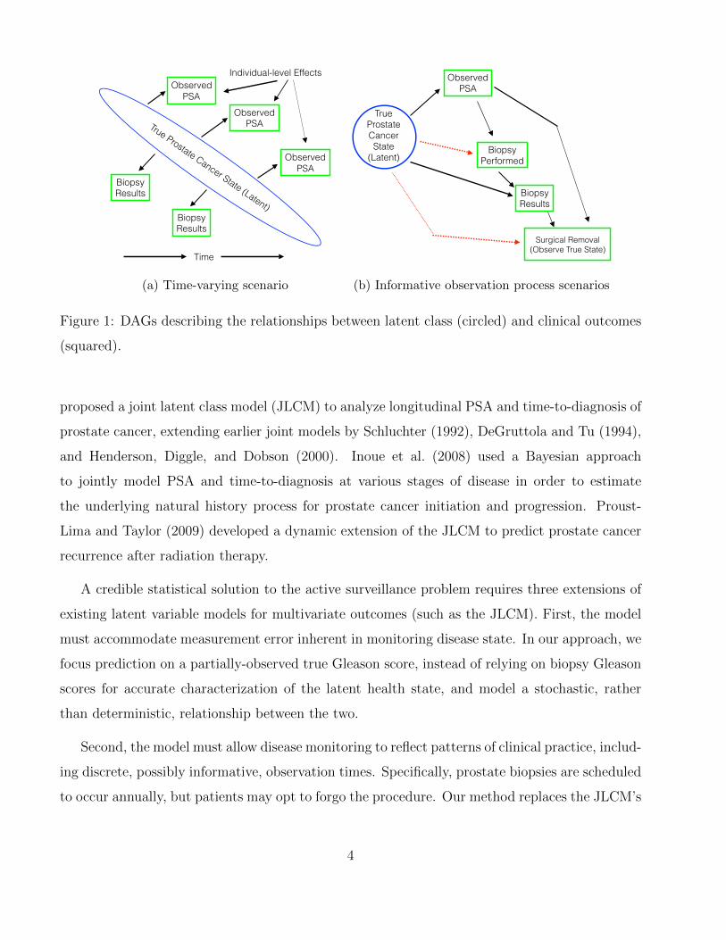
An individual’s cancer state is assumed to be manifest in both the level and trajectory of
PSA measurements as well as in the outcomes from repeated biopsies. These relationships are
illustrated by the directed acyclic graph (DAG) in Figure 1(a). In the model we are proposing,
PSA measurements follow a multilevel model with mean intercept and age effects varying across
latent classes. Then, repeated annual biopsies constitute a time-to-event outcome since patients
exit AS after grade reclassification on biopsy. So, time until reclassification on biopsy is modeled
using pooled logistic regression under the assumption that biopsy results are independent condi-
tional on cancer state and covariates (Cupples et al., 1988). Pooled logistic regression provides
survival estimates equivalent to those of a time-varying Cox model for discrete event times and
conditionally independent intervals (D’Agostino et al., 1990). As indicated in Figure 1(a), PSA
and biopsy results are also assumed to be conditionally independent given latent class.
The model depicted in Figure 1(a) is related to previous work by Lin et al. (2002), who
3
True Prostate Cancer State (Latent)
Observed PSA
Observed PSA
Observed PSA
Biopsy Results
Biopsy Results
Individual-level Effects
Time
(a) Time-varying scenario
Surgical Removal (Observe True State)
True Prostate Cancer State
(Latent)
Biopsy Results
Observed PSA
Biopsy Performed
(b) Informative observation process scenarios
Figure 1: DAGs describing the relationships between latent class (circled) and clinical outcomes
(squared).
proposed a joint latent class model (JLCM) to analyze longitudinal PSA and time-to-diagnosis of
prostate cancer, extending earlier joint models by Schluchter (1992), DeGruttola and Tu (1994),
and Henderson, Diggle, and Dobson (2000). Inoue et al. (2008) used a Bayesian approach
to jointly model PSA and time-to-diagnosis at various stages of disease in order to estimate
the underlying natural history process for prostate cancer initiation and progression. Proust-
Lima and Taylor (2009) developed a dynamic extension of the JLCM to predict prostate cancer
recurrence after radiation therapy.
A credible statistical solution to the active surveillance problem requires three extensions of
existing latent variable models for multivariate outcomes (such as the JLCM). First, the model
must accommodate measurement error inherent in monitoring disease state. In our approach, we
focus prediction on a partially-observed true Gleason score, instead of relying on biopsy Gleason
scores for accurate characterization of the latent health state, and model a stochastic, rather
than deterministic, relationship between the two.
Second, the model must allow disease monitoring to reflect patterns of clinical practice, includ-
ing discrete, possibly informative, observation times. Specifically, prostate biopsies are scheduled
to occur annually, but patients may opt to forgo the procedure. Our method replaces the JLCM’s
4
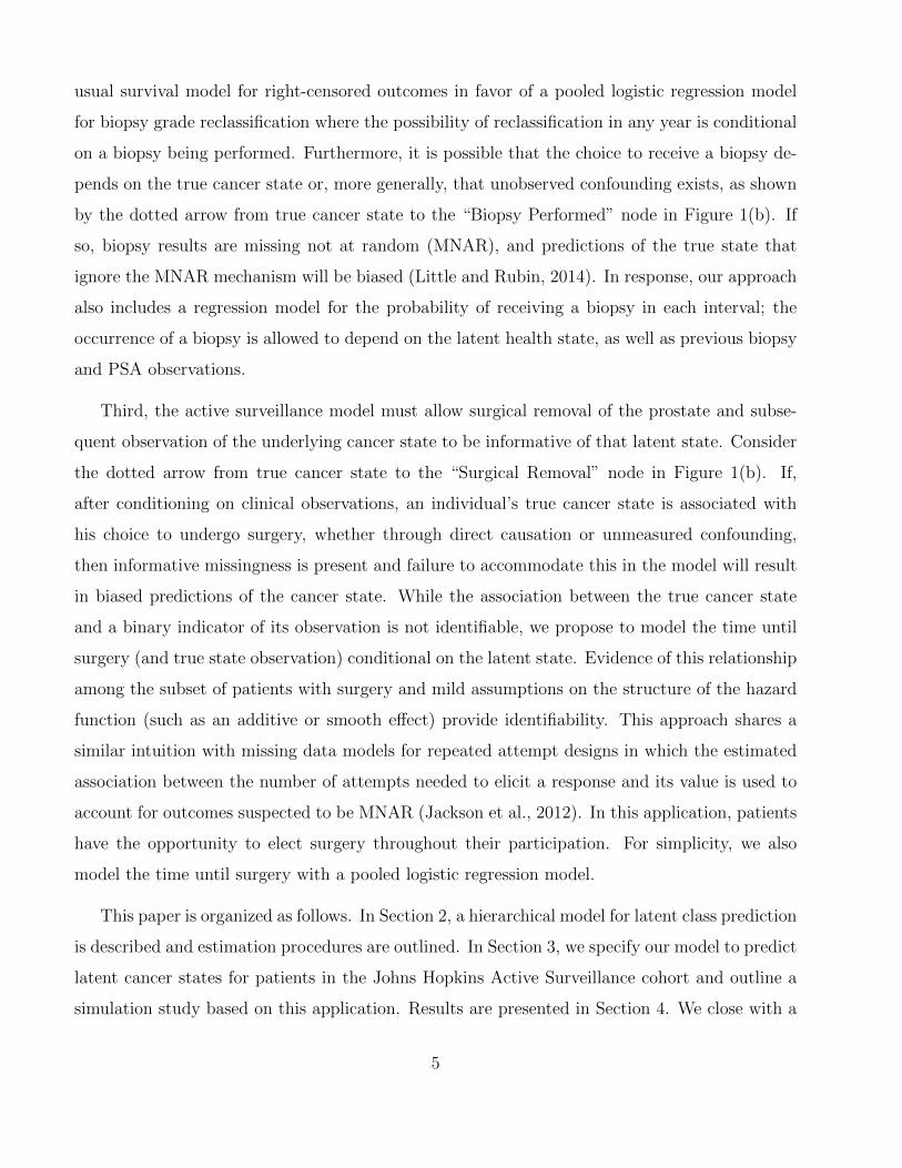
usual survival model for right-censored outcomes in favor of a pooled logistic regression model
for biopsy grade reclassification where the possibility of reclassification in any year is conditional
on a biopsy being performed. Furthermore, it is possible that the choice to receive a biopsy de-
pends on the true cancer state or, more generally, that unobserved confounding exists, as shown
by the dotted arrow from true cancer state to the “Biopsy Performed” node in Figure 1(b). If
so, biopsy results are missing not at random (MNAR), and predictions of the true state that
ignore the MNAR mechanism will be biased (Little and Rubin, 2014). In response, our approach
also includes a regression model for the probability of receiving a biopsy in each interval; the
occurrence of a biopsy is allowed to depend on the latent health state, as well as previous biopsy
and PSA observations.
Third, the active surveillance model must allow surgical removal of the prostate and subse-
quent observation of the underlying cancer state to be informative of that latent state. Consider
the dotted arrow from true cancer state to the “Surgical Removal” node in Figure 1(b). If,
after conditioning on clinical observations, an individual’s true cancer state is associated with
his choice to undergo surgery, whether through direct causation or unmeasured confounding,
then informative missingness is present and failure to accommodate this in the model will result
in biased predictions of the cancer state. While the association between the true cancer state
and a binary indicator of its observation is not identifiable, we propose to model the time until
surgery (and true state observation) conditional on the latent state. Evidence of this relationship
among the subset of patients with surgery and mild assumptions on the structure of the hazard
function (such as an additive or smooth effect) provide identifiability. This approach shares a
similar intuition with missing data models for repeated attempt designs in which the estimated
association between the number of attempts needed to elicit a response and its value is used to
account for outcomes suspected to be MNAR (Jackson et al., 2012). In this application, patients
have the opportunity to elect surgery throughout their participation. For simplicity, we also
model the time until surgery with a pooled logistic regression model.
This paper is organized as follows. In Section 2, a hierarchical model for latent class prediction
is described and estimation procedures are outlined. In Section 3, we specify our model to predict
latent cancer states for patients in the Johns Hopkins Active Surveillance cohort and outline a
simulation study based on this application. Results are presented in Section 4. We close with a
5
discussion.
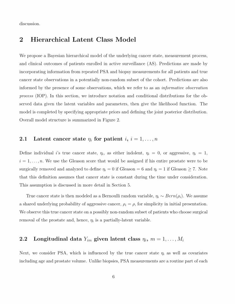
2 Hierarchical Latent Class Model
We propose a Bayesian hierarchical model of the underlying cancer state, measurement process,
and clinical outcomes of patients enrolled in active surveillance (AS). Predictions are made by
incorporating information from repeated PSA and biopsy measurements for all patients and true
cancer state observations in a potentially non-random subset of the cohort. Predictions are also
informed by the presence of some observations, which we refer to as an informative observation
process (IOP). In this section, we introduce notation and conditional distributions for the ob-
served data given the latent variables and parameters, then give the likelihood function. The
model is completed by specifying appropriate priors and defining the joint posterior distribution.
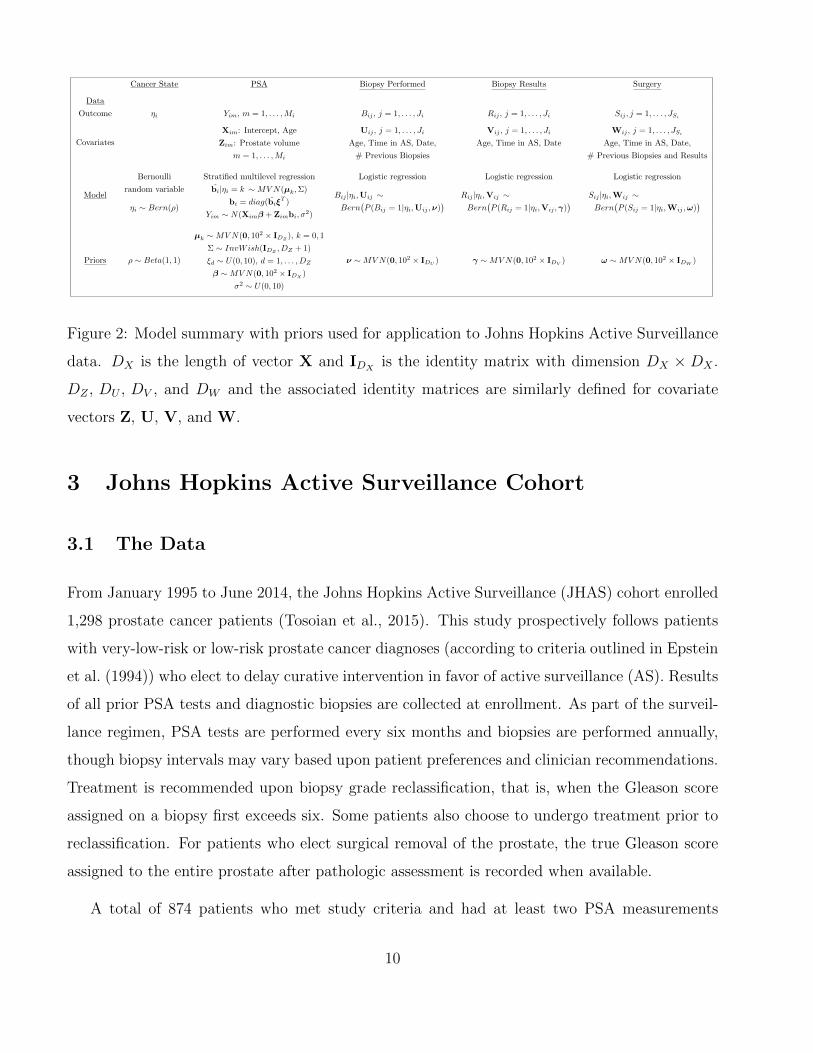
Overall model structure is summarized in Figure 2.
2.1 Latent cancer state ηi for patient i, i = 1, . . . , n
Define individual i’s true cancer state, ηi, as either indolent, ηi = 0, or aggressive, ηi = 1,
i = 1, . . . , n. We use the Gleason score that would be assigned if his entire prostate were to be
surgically removed and analyzed to define ηi = 0 if Gleason = 6 and ηi = 1 if Gleason ≥ 7. Note
that this definition assumes that cancer state is constant during the time under consideration.
This assumption is discussed in more detail in Section 5.
True cancer state is then modeled as a Bernoulli random variable, ηi ∼ Bern(ρi). We assume
a shared underlying probability of aggressive cancer, ρi = ρ, for simplicity in initial presentation.
We observe this true cancer state on a possibly non-random subset of patients who choose surgical
removal of the prostate and, hence, ηi is a partially-latent variable.
2.2 Longitudinal data Yim given latent class ηi, m = 1, . . . ,Mi
Next, we consider PSA, which is influenced by the true cancer state ηi as well as covariates
including age and prostate volume. Unlike biopsies, PSA measurements are a routine part of each
6
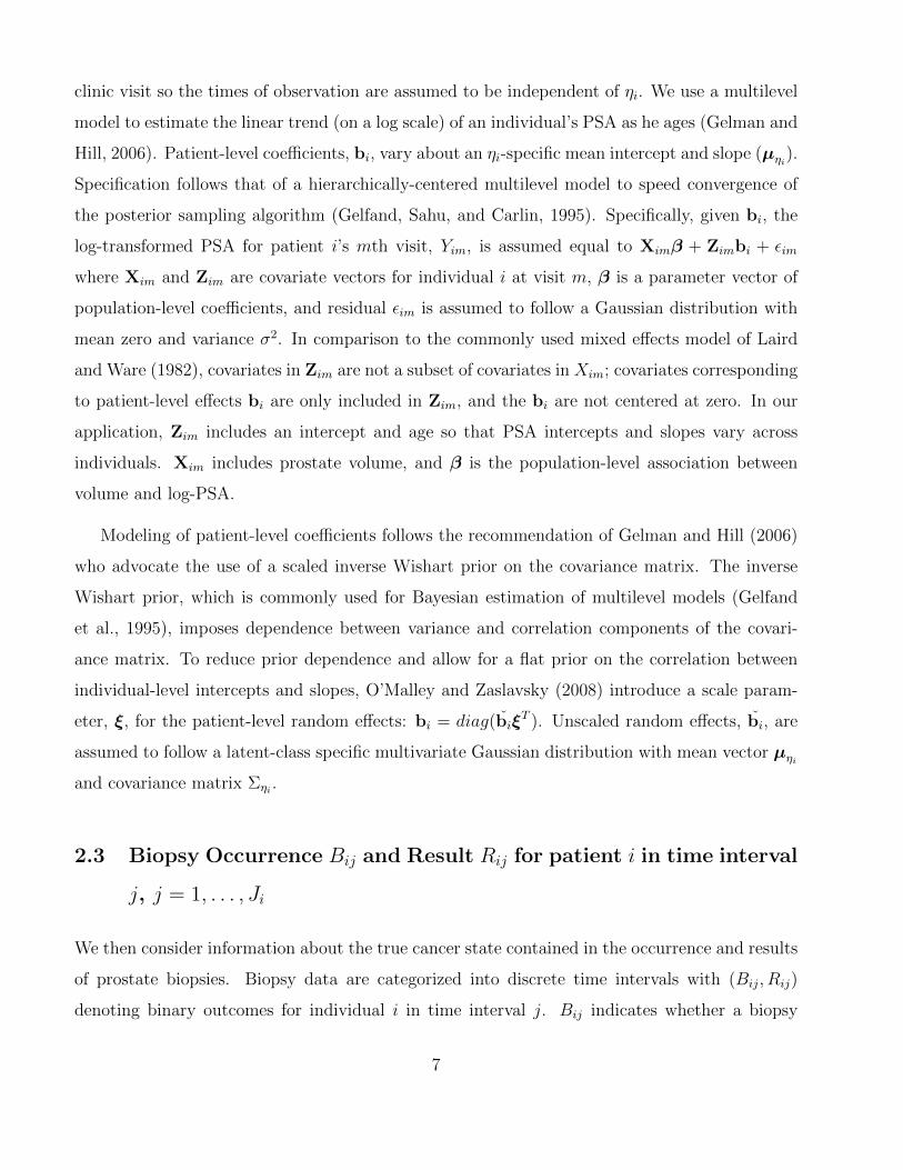
clinic visit so the times of observation are assumed to be independent of ηi. We use a multilevel
model to estimate the linear trend (on a log scale) of an individual’s PSA as he ages (Gelman and
Hill, 2006). Patient-level coefficients, bi, vary about an ηi-specific mean intercept and slope (µηi).
Specification follows that of a hierarchically-centered multilevel model to speed convergence of
the posterior sampling algorithm (Gelfand, Sahu, and Carlin, 1995). Specifically, given bi, the
log-transformed PSA for patient i’s mth visit, Yim, is assumed equal to Ximβ + Zimbi + εim
where Xim and Zim are covariate vectors for individual i at visit m, β is a parameter vector of
population-level coefficients, and residual εim is assumed to follow a Gaussian distribution with
mean zero and variance σ2. In comparison to the commonly used mixed effects model of Laird
and Ware (1982), covariates in Zim are not a subset of covariates in Xim; covariates corresponding
to patient-level effects bi are only included in Zim, and the bi are not centered at zero. In our
application, Zim includes an intercept and age so that PSA intercepts and slopes vary across
individuals. Xim includes prostate volume, and β is the population-level association between
volume and log-PSA.
Modeling of patient-level coefficients follows the recommendation of Gelman and Hill (2006)
who advocate the use of a scaled inverse Wishart prior on the covariance matrix. The inverse
Wishart prior, which is commonly used for Bayesian estimation of multilevel models (Gelfand
et al., 1995), imposes dependence between variance and correlation components of the covari-
ance matrix. To reduce prior dependence and allow for a flat prior on the correlation between
individual-level intercepts and slopes, O’Malley and Zaslavsky (2008) introduce a scale param-
eter, ξ, for the patient-level random effects: bi = diag(biξT ). Unscaled random effects, bi, are
assumed to follow a latent-class specific multivariate Gaussian distribution with mean vector µηi
and covariance matrix Σηi .
2.3 Biopsy Occurrence Bij and Result Rij for patient i in time interval
j, j = 1, . . . , Ji
We then consider information about the true cancer state contained in the occurrence and results
of prostate biopsies. Biopsy data are categorized into discrete time intervals with (Bij, Rij)
denoting binary outcomes for individual i in time interval j. Bij indicates whether a biopsy
7
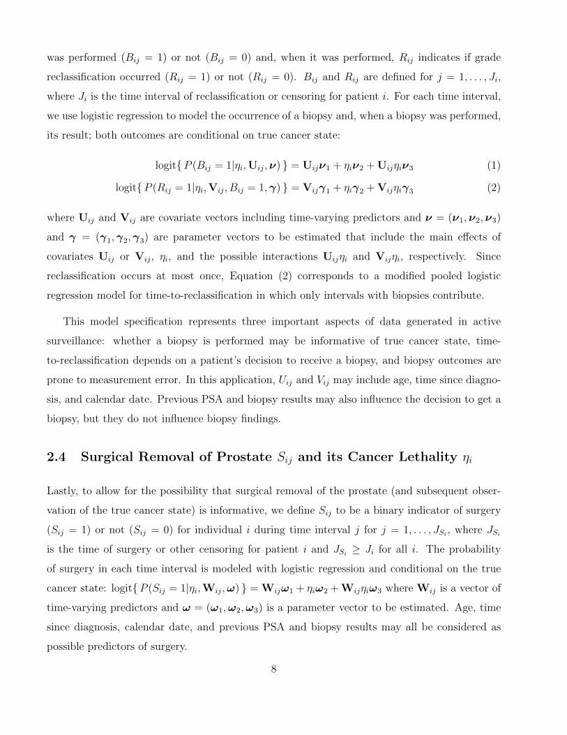
was performed (Bij = 1) or not (Bij = 0) and, when it was performed, Rij indicates if grade
reclassification occurred (Rij = 1) or not (Rij = 0). Bij and Rij are defined for j = 1, . . . , Ji,
where Ji is the time interval of reclassification or censoring for patient i. For each time interval,
we use logistic regression to model the occurrence of a biopsy and, when a biopsy was performed,
its result; both outcomes are conditional on true cancer state:
logit{P (Bij = 1|ηi,Uij,ν) } = Uijν1 + ηiν2 + Uijηiν3 (1)
logit{P (Rij = 1|ηi,Vij, Bij = 1,γ) } = Vijγ1 + ηiγ2 + Vijηiγ3 (2)
where Uij and Vij are covariate vectors including time-varying predictors and ν = (ν1,ν2,ν3)
and γ = (γ1,γ2,γ3) are parameter vectors to be estimated that include the main effects of
covariates Uij or Vij, ηi, and the possible interactions Uijηi and Vijηi, respectively. Since
reclassification occurs at most once, Equation (2) corresponds to a modified pooled logistic
regression model for time-to-reclassification in which only intervals with biopsies contribute.
This model specification represents three important aspects of data generated in active
surveillance: whether a biopsy is performed may be informative of true cancer state, time-
to-reclassification depends on a patient’s decision to receive a biopsy, and biopsy outcomes are
prone to measurement error. In this application, Uij and Vij may include age, time since diagno-
sis, and calendar date. Previous PSA and biopsy results may also influence the decision to get a
biopsy, but they do not influence biopsy findings.
2.4 Surgical Removal of Prostate Sij and its Cancer Lethality ηi
Lastly, to allow for the possibility that surgical removal of the prostate (and subsequent obser-
vation of the true cancer state) is informative, we define Sij to be a binary indicator of surgery
(Sij = 1) or not (Sij = 0) for individual i during time interval j for j = 1, . . . , JSi, where JSi
is the time of surgery or other censoring for patient i and JSi≥ Ji for all i. The probability
of surgery in each time interval is modeled with logistic regression and conditional on the true
cancer state: logit{P (Sij = 1|ηi,Wij,ω) } = Wijω1 + ηiω2 + Wijηiω3 where Wij is a vector of
time-varying predictors and ω = (ω1,ω2,ω3) is a parameter vector to be estimated. Age, time
since diagnosis, calendar date, and previous PSA and biopsy results may all be considered as
possible predictors of surgery.
8
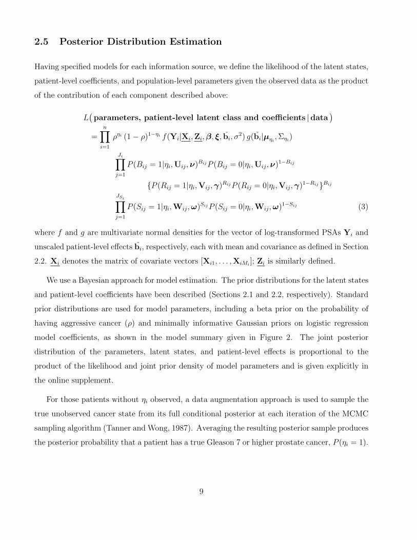
2.5 Posterior Distribution Estimation
Having specified models for each information source, we define the likelihood of the latent states,
patient-level coefficients, and population-level parameters given the observed data as the product
of the contribution of each component described above:
L(parameters, patient-level latent class and coefficients |data
)
=n∏
i=1
ρηi (1− ρ)1−ηi f(Yi|Xi,Zi,β, ξ, bi, σ2) g(bi|µηi ,Σηi)
Ji∏
j=1
P (Bij = 1|ηi,Uij,ν)BijP (Bij = 0|ηi,Uij,ν)1−Bij
{P (Rij = 1|ηi,Vij,γ)RijP (Rij = 0|ηi,Vij,γ)1−Rij}Bij
JSi∏
j=1
P (Sij = 1|ηi,Wij,ω)SijP (Sij = 0|ηi,Wij,ω)1−Sij (3)
where f and g are multivariate normal densities for the vector of log-transformed PSAs Yi and
unscaled patient-level effects bi, respectively, each with mean and covariance as defined in Section
2.2. Xi denotes the matrix of covariate vectors [Xi1, . . . ,XiMi]; Zi is similarly defined.
We use a Bayesian approach for model estimation. The prior distributions for the latent states
and patient-level coefficients have been described (Sections 2.1 and 2.2, respectively). Standard
prior distributions are used for model parameters, including a beta prior on the probability of
having aggressive cancer (ρ) and minimally informative Gaussian priors on logistic regression
model coefficients, as shown in the model summary given in Figure 2. The joint posterior
distribution of the parameters, latent states, and patient-level effects is proportional to the
product of the likelihood and joint prior density of model parameters and is given explicitly in
the online supplement.
For those patients without ηi observed, a data augmentation approach is used to sample the
true unobserved cancer state from its full conditional posterior at each iteration of the MCMC
sampling algorithm (Tanner and Wong, 1987). Averaging the resulting posterior sample produces
the posterior probability that a patient has a true Gleason 7 or higher prostate cancer, P (ηi = 1).
9
Cancer State PSA Biopsy Performed Biopsy Results Surgery
Data
Outcome ⌘i Yim, m = 1, . . . , Mi Bij , j = 1, . . . , Ji Rij , j = 1, . . . , Ji Sij , j = 1, . . . , JSi
Covariates
Xim: Intercept, Age Uij , j = 1, . . . , Ji Vij , j = 1, . . . , Ji Wij , j = 1, . . . , JSi
Zim: Prostate volume Age, Time in AS, Date, Age, Time in AS, Date Age, Time in AS, Date,
m = 1, . . . , Mi # Previous Biopsies # Previous Biopsies and Results
Model
Bernoulli Stratified multilevel regression Logistic regression Logistic regression Logistic regression
random variable bi|⌘i = k ⇠ MV N(µk,⌃)Bij |⌘i,Uij ⇠ Rij |⌘i,Vij ⇠ Sij |⌘i,Wij ⇠
⌘i ⇠ Bern(⇢)bi = diag(bi⇠
T )Bern
�P (Bij = 1|⌘i,Uij ,⌫)
�Bern
�P (Rij = 1|⌘i,Vij ,�)
�Bern
�P (Sij = 1|⌘i,Wij ,!)
�Yim ⇠ N(Xim� + Zimbi,�
2)
Priors ⇢ ⇠ Beta(1, 1)
µk ⇠ MV N(0, 102 ⇥ IDZ), k = 0, 1
⌫ ⇠ MV N(0, 102 ⇥ IDU) � ⇠ MV N(0, 102 ⇥ IDV
) ! ⇠ MV N(0, 102 ⇥ IDW)
⌃ ⇠ InvWish(IDZ, DZ + 1)
⇠d ⇠ U(0, 10), d = 1, . . . , DZ
� ⇠ MV N(0, 102 ⇥ IDX)
�2 ⇠ U(0, 10)
Figure 2: Model summary with priors used for application to Johns Hopkins Active Surveillance
data. DX is the length of vector X and IDXis the identity matrix with dimension DX × DX .
DZ , DU , DV , and DW and the associated identity matrices are similarly defined for covariate
vectors Z, U, V, and W.
3 Johns Hopkins Active Surveillance Cohort
3.1 The Data
From January 1995 to June 2014, the Johns Hopkins Active Surveillance (JHAS) cohort enrolled
1,298 prostate cancer patients (Tosoian et al., 2015). This study prospectively follows patients
with very-low-risk or low-risk prostate cancer diagnoses (according to criteria outlined in Epstein
et al. (1994)) who elect to delay curative intervention in favor of active surveillance (AS). Results
of all prior PSA tests and diagnostic biopsies are collected at enrollment. As part of the surveil-
lance regimen, PSA tests are performed every six months and biopsies are performed annually,
though biopsy intervals may vary based upon patient preferences and clinician recommendations.
Treatment is recommended upon biopsy grade reclassification, that is, when the Gleason score
assigned on a biopsy first exceeds six. Some patients also choose to undergo treatment prior to
reclassification. For patients who elect surgical removal of the prostate, the true Gleason score
assigned to the entire prostate after pathologic assessment is recorded when available.
A total of 874 patients who met study criteria and had at least two PSA measurements
10
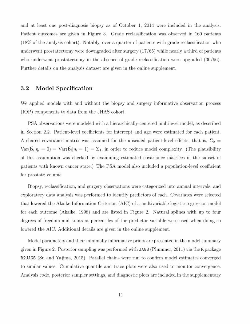
and at least one post-diagnosis biopsy as of October 1, 2014 were included in the analysis.
Patient outcomes are given in Figure 3. Grade reclassification was observed in 160 patients
(18% of the analysis cohort). Notably, over a quarter of patients with grade reclassification who
underwent prostatectomy were downgraded after surgery (17/65) while nearly a third of patients
who underwent prostatectomy in the absence of grade reclassification were upgraded (30/96).
Further details on the analysis dataset are given in the online supplement.
3.2 Model Specification
We applied models with and without the biopsy and surgery informative observation process
(IOP) components to data from the JHAS cohort.
PSA observations were modeled with a hierarchically-centered multilevel model, as described
in Section 2.2. Patient-level coefficients for intercept and age were estimated for each patient.
A shared covariance matrix was assumed for the unscaled patient-level effects, that is, Σ0 =
Var(bi|ηi = 0) = Var(bi|ηi = 1) = Σ1, in order to reduce model complexity. (The plausibility
of this assumption was checked by examining estimated covariance matrices in the subset of
patients with known cancer state.) The PSA model also included a population-level coefficient
for prostate volume.
Biopsy, reclassification, and surgery observations were categorized into annual intervals, and
exploratory data analysis was performed to identify predictors of each. Covariates were selected
that lowered the Akaike Information Criterion (AIC) of a multivariable logistic regression model
for each outcome (Akaike, 1998) and are listed in Figure 2. Natural splines with up to four
degrees of freedom and knots at percentiles of the predictor variable were used when doing so
lowered the AIC. Additional details are given in the online supplement.
Model parameters and their minimally informative priors are presented in the model summary
given in Figure 2. Posterior sampling was performed with JAGS (Plummer, 2011) via the R package
R2JAGS (Su and Yajima, 2015). Parallel chains were run to confirm model estimates converged
to similar values. Cumulative quantile and trace plots were also used to monitor convergence.
Analysis code, posterior sampler settings, and diagnostic plots are included in the supplementary
11
n=874
Grade Reclassificationn=160
No Grade Reclassificationn=714
Surgeryn=67
Other Treatmentn=69
No Treatmentn=24
Surgeryn=100
Other Treatmentn=82
Lost toFollow-up
n=106
Deathn=19
Activen=407
TrueGS = 6n= 17
TrueGS > 6n= 48
TrueGS = 6n= 66
TrueGS > 6n= 30
Figure 3: CONSORT diagram for Johns Hopkins Active Surveillance prospective cohort patients
included in this analysis. Post-surgery full prostate Gleason score (GS) observations are also
given (circled). (Six patients who underwent prostatectomy did not have true GS observations
available.)
12
material.
3.3 Model Assessment
Predictive accuracy was assessed among patients with post-surgery true Gleason score obser-
vations. Out-of-sample posterior predictions of η were obtained for each patient by removing
his true state observation from the analysis dataset and re-running the posterior sampler with
an additional data augmentation step for the patient of interest. Out-of-sample predictions of
ηi were then compared to known values with receiver operating characteristic (ROC) curves
(Hanley and McNeil, 1982) and calibration plots (Steyerberg et al., 2010). For the former, the
area under the curve (AUC) and associated 95% bootstrapped intervals were calculated. For
the latter, a plot comparing posterior predictions to observed rates of class membership was
constructed by performing logistic regression of the observed true state on a natural spline rep-
resentation of out-of-sample posterior predictions (degrees of freedom = 2). The mean squared
error (MSE) between observed and predicted cancer state was also calculated. For comparison,
posterior predictions were obtained from a logistic regression model fit with data from patients
with post-surgery observations of η; covariates included age, time since diagnosis, and PSA and
biopsy results. We also compared specificity of model predictions to the specificity of using final
biopsy results to predict the true cancer state by fixing sensitivity at the observed true positive
rate of biopsy Gleason score (dichotomized < 7 or ≥ 7).
Calibration plots were also drawn to assess model fit for outcomes observed on all patients:
the occurrence of a biopsy, grade reclassification on biopsy, and the occurrence of surgery. Code
for reproducing all plots is available in the supplementary material.
3.4 Simulations
We performed a simulation study to examine model performance in this application. 200 sim-
ulated datasets were generated using posterior estimates of model parameters obtained from
the biopsy and surgery IOP analysis of JHAS data. For each dataset, the proposed model was
estimated under four settings: unadjusted (no IOP components), biopsy IOP only, surgery IOP
13
only, and both biopsy and surgery IOP components. Posterior predictions of the latent state
were obtained for all simulated patients and compared to known (data-generating) values. For
patients without surgery, posterior samples of η were generated with a data augmentation step
as a matter of course in model estimation. For patients with surgery, the posterior probability
of η = 1 was estimated via an importance sampling algorithm performed on the joint posterior
(Bishop et al., 2006), which is less computationally intensive than the out-of-sample methods
used in Section 3.3. (See technical report of Fisher et al. (2015) for further details.) Posterior
predictions of η were also compared to fitted probabilities from a logistic regression model. Code
for generating data, estimating the joint posterior, and obtaining predictions is included in the
supplementary material.
4 Results
The estimated marginal probability of harboring a prostate cancer with Gleason score above
7 was 0.23 (95% CI: 0.16, 0.33) for the proposed model with biopsy and surgery IOP compo-
nents, 0.20 (0.14, 0.28) with surgery IOP only, 0.31 (0.24, 0.39) with biopsy IOP only and 0.30
(0.23, 0.38) with no IOP components. Patients with η = 1 were less likely to receive biopsies–
leading to underestimation of ρ in models without the biopsy IOP component–and more likely
to elect surgery, such that ρ was overestimated when not accounting for informative observation.
Parameter estimates and credible intervals from all models are given in the online supplement
(Appendix Tables A3-A7).
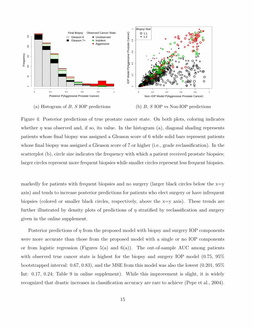
A histogram of predictions of η from the model with biopsy and surgery IOP components is
given in Figure 4(a). Patients with posterior predictions above 60% are primarily those who both
experienced grade reclassification (solid bars) and elected prostatectomy (red and green). 95%
of AS patients who neither reclassified (diagonal shading) nor underwent surgery (black) have
posterior predictions that are lower than 50%; a majority have predictions below 20%. Figure
4(b) shows a scatterplot comparing posterior probabilities of aggressive cancer, P (η = 1), between
models with and without IOP components. The models produce similar posterior predictions
for most patients, particularly those patients for which the non-IOP model assigns very low
risk. Inclusion of biopsy and surgery IOP components decreases posterior predictions of η most
14
Posterior P(Aggressive Prostate Cancer)
Fre
quen
cy
0 0.2 0.4 0.6 0.8 1
050
100
150
200
250
Observed Cancer State
UnobservedIndolentAggressive
Final Biopsy
Gleason 6Gleason 7+
(a) Histogram of B, S IOP predictions
●
●
●
●●
●
●
●●
●●
●
●
●
●
●
●
●
●
●
●
●●
●
●●
●
●
●
●
●●
●
●
●
●
●
●
●
●
●
●
●
●
●
●
●
●
●●
●
●
●
●●
●
●
●
●
●
● ●●
●
●
●
●
●
●
●
●
●
●
●
●
●
●
●
●
●
●
●
●●●
●
●
●
● ●
●
●
●
●
●
●
●
●
●●
●
●
●
●
●
●
●
●
●
●
●
●
●
●
●
●
●
●●
●
●
●
●
●
●●
●
●
●
●
●●
●
●
●
●
●
●
●
●
●
●
●●
● ●
●
●●●
●
●●
●
●
●
●
●
●
●
●
●●
●
●
●
●
●
●
●
●
●
●
●
●●
●
●
●
●
●
●
●
●
●
●
●
●
●
●
●
●
●
●
●
●
●
●
●
●
●
●
●
●
●
●
●
●
●
●
●
●
●
●●
●
●
●
●●
●
●
●
●
●
●
●
●
●●
● ●
●
●
●
●
●
●
●
●
●●
●●
●
●
●
●
●
●●
●
●
●
●
●
●
●
●
●
●
●
●
●
●
● ●
●
●
●
●
●
●
●
●
●
●
●
●
●
●
●
●
●
●
●
●
●●
●
●
●
●
●
●● ●
●
●
●
●●
●
●
●
● ●●
●●
●
●●
●●
●
●●
●
●
●
●
●
●
●
●
●●
●
●
●
●
●
● ●
●●
●●
●
●
●
●●
●
●
●
●
●
●
●
● ●●
●
●
●
●●
●
●
●
●
● ●●
●
●●
●
●
●
●●
●
●
●
●●
●
●
●
●
●
●
●●
●
●
●
●
●
●
●
●
●
●
●
●●●
●
●
●
●
●
●
●
●
●
●
●
●
●
●
●
●
●
●
●
●
●●
●
●
●
●●●
●
●
●
●
●
●
●●
●
●
●
●
●
●●
●
●
●
●
●●
●
●
●
●
●
●
●
●
● ●
●
●
●
●
●
●
●
●●●
●
●
●
●
●
●
●
●
●
●
●
●
●●
●
●
●
●
●
●
●
●
●● ●●
●
●
●
●
●
●
●
●
●
●
●
●
●
●
●
●
●
●
●
●
●
●
●●
●
●
●
●
●
●
●●
●●
●
●
●●
●
●
●
●
●●
●
●
●
●●
●
●●
●
●
●●●●
●
●
●
●●
●
●
●
●
●
●
●
● ●
●
●●
●
●
●
●
●
● ●
●
●
●
●
●
●
●
●
●
●
●
●
●●
●
●●
●
●
●
●
●
●
●
●
●
●
●
●●
●
●
●
●
●
●
●
●
●
●
●●
●
●●
●
●●
●
●
●
●
●
●
●
●
●
●
●
●
●●
●●
●
●
●
●
●●●
●
●
●
●
●
●● ●
●
●
●
●
●
●
●
●
●
●
●
●
●
●
●
●
●
●
●
●
●
●
●
●
●
●
●
●●
●
●
●
●
●
●
●
●
●
●
●
●
●
●●
●
●● ●
●
●
●
●
●
●
●
●
●●
●
●●
●●
●
●
●
●
●
●●
●
●
●●
●
●
●
●
●
●
●
●
●
●
●
●
●●
●●
●
●
●
●
●●
●
●
●
●
●
●
●
●
●
●
●
●●
●
●
●
●
● ●●●
●
●●
●●
●
●
●
●●
●
●
●
●
●
●
●
●
●
●
●
●
●
●
●
●
●●
●
●
●
●
●
●
●
●
●
●
●
●
●
●
●
●
●
●
●●
●●
●
●
●
●
●
●
●●
●
●
●
●
●
●
●●
●●
●
● ●
●
●●
●●
●
●
●
●●
●
●
●
●
●
●
●
●
●
●
●
●●●
●
●●
●●
Non−IOP Model P(Aggressive Prostate Cancer)
IOP
Mod
el P
(Agg
ress
ive
Pro
stat
e C
ance
r)
0 0.2 0.4 0.6 0.8 1
00.
20.
40.
60.
81
●
●
●
●●
●
●
●●
●●
●
●
●
●
●
●
●
●
●
●
●●
●
●●
●
●
●
●
●●
●
●
●
●
●
●
●
●
●
●
●
●
●
●
●
●
●●
●
●
●
●●
●
●
●
●
●
● ●●
●
●
●
●
●
●
●
●
●
●
●
●
●
●
●
●
●
●
●
●●●
●
●
●
● ●
●
●
●
●
●
●
●
●
●●
●
●
●
●
●
●
●
●
●
●
●
●
●
●
●
●
●
●●
●
●
●
●
●
●●
●
●
●
●
●●
●
●
●
●
●
●
●
●
●
●
●●
● ●
●
●●●
●
●●
●
●
●
●
●
●
●
●
●
●
Biopsy:Year
1:11:2
(b) B, S IOP vs Non-IOP predictions
Figure 4: Posterior predictions of true prostate cancer state. On both plots, coloring indicates
whether η was observed and, if so, its value. In the histogram (a), diagonal shading represents
patients whose final biopsy was assigned a Gleason score of 6 while solid bars represent patients
whose final biopsy was assigned a Gleason score of 7 or higher (i.e., grade reclassification). In the
scatterplot (b), circle size indicates the frequency with which a patient received prostate biopsies;
larger circles represent more frequent biopsies while smaller circles represent less frequent biopsies.
markedly for patients with frequent biopsies and no surgery (larger black circles below the x=y
axis) and tends to increase posterior predictions for patients who elect surgery or have infrequent
biopsies (colored or smaller black circles, respectively, above the x=y axis). These trends are
further illustrated by density plots of predictions of η stratified by reclassification and surgery
given in the online supplement.
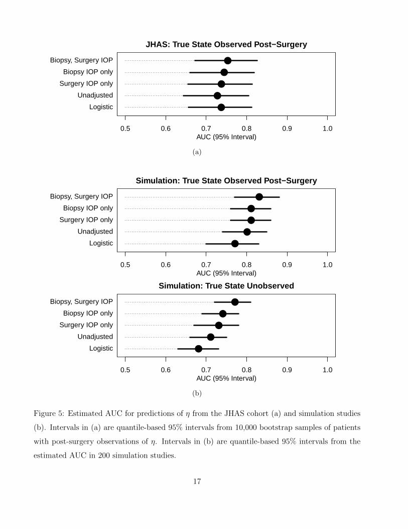
Posterior predictions of η from the proposed model with biopsy and surgery IOP components
were more accurate than those from the proposed model with a single or no IOP components
or from logistic regression (Figures 5(a) and 6(a)). The out-of-sample AUC among patients
with observed true cancer state is highest for the biopsy and surgery IOP model (0.75, 95%
bootstrapped interval: 0.67, 0.83), and the MSE from this model was also the lowest (0.201, 95%
Int: 0.17, 0.24; Table 9 in online supplement). While this improvement is slight, it is widely
recognized that drastic increases in classification accuracy are rare to achieve (Pepe et al., 2004).
15
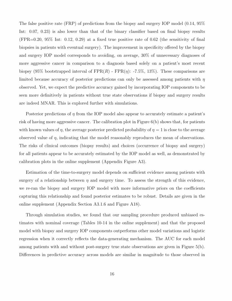
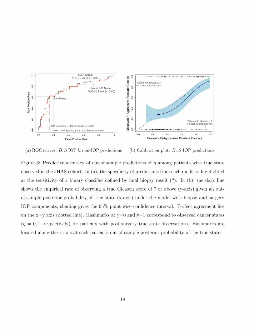
The false positive rate (FRP) of predictions from the biopsy and surgery IOP model (0.14, 95%
Int: 0.07, 0.23) is also lower than that of the binary classifier based on final biopsy results
(FPR=0.20, 95% Int: 0.12, 0.29) at a fixed true positive rate of 0.62 (the sensitivity of final
biopsies in patients with eventual surgery). The improvement in specificity offered by the biopsy
and surgery IOP model corresponds to avoiding, on average, 30% of unnecessary diagnoses of
more aggressive cancer in comparison to a diagnosis based solely on a patient’s most recent
biopsy (95% bootstrapped interval of FPR(R) - FPR(η): -7.5%, 13%). These comparisons are
limited because accuracy of posterior predictions can only be assessed among patients with η
observed. Yet, we expect the predictive accuracy gained by incorporating IOP components to be
seen more definitively in patients without true state observations if biopsy and surgery results
are indeed MNAR. This is explored further with simulations.
Posterior predictions of η from the IOP model also appear to accurately estimate a patient’s
risk of having more aggressive cancer. The calibration plot in Figure 6(b) shows that, for patients
with known values of η, the average posterior predicted probability of η = 1 is close to the average
observed value of η, indicating that the model reasonably reproduces the mean of observations.
The risks of clinical outcomes (biopsy results) and choices (occurrence of biopsy and surgery)
for all patients appear to be accurately estimated by the IOP model as well, as demonstrated by
calibration plots in the online supplement (Appendix Figure A3).
Estimation of the time-to-surgery model depends on sufficient evidence among patients with
surgery of a relationship between η and surgery time. To assess the strength of this evidence,
we re-ran the biopsy and surgery IOP model with more informative priors on the coefficients
capturing this relationship and found posterior estimates to be robust. Details are given in the
online supplement (Appendix Section A3.1.6 and Figure A18).
Through simulation studies, we found that our sampling procedure produced unbiased es-
timates with nominal coverage (Tables 10-14 in the online supplement) and that the proposed
model with biopsy and surgery IOP components outperforms other model variations and logistic
regression when it correctly reflects the data-generating mechanism. The AUC for each model
among patients with and without post-surgery true state observations are given in Figure 5(b).
Differences in predictive accuracy across models are similar in magnitude to those observed in
16
0.5 0.6 0.7 0.8 0.9 1.0
JHAS: True State Observed Post−Surgery
AUC (95% Interval)
Biopsy, Surgery IOP
Biopsy IOP only
Surgery IOP only
Unadjusted
Logistic
●
●
●
●
●
(a)
0.5 0.6 0.7 0.8 0.9 1.0
Simulation: True State Observed Post−Surgery
AUC (95% Interval)
Biopsy, Surgery IOP
Biopsy IOP only
Surgery IOP only
Unadjusted
Logistic
●
●
●
●
●
0.5 0.6 0.7 0.8 0.9 1.0
Simulation: True State Unobserved
AUC (95% Interval)
Biopsy, Surgery IOP
Biopsy IOP only
Surgery IOP only
Unadjusted
Logistic
●
●
●
●
●
(b)
Figure 5: Estimated AUC for predictions of η from the JHAS cohort (a) and simulation studies
(b). Intervals in (a) are quantile-based 95% intervals from 10,000 bootstrap samples of patients
with post-surgery observations of η. Intervals in (b) are quantile-based 95% intervals from the
estimated AUC in 200 simulation studies.
17
Non - I.O.P. Specificity = 81% at Sensitivity = 62%
I.O.P. Specificity = 86% at Sensitivity = 62%
I.O.P. Model AUC= 0.75 (0.67, 0.83)
Non-I.O.P. Model AUC= 0.73 (0.64, 0.80)
Last Biopsy
False Positive Rate
True
Pos
itive
Rat
e
0.0 0.2 0.4 0.6 0.8 1.0
0.0
0.2
0.4
0.6
0.8
1.0
*
(a) ROC curves: B,S IOP & non-IOP predictions
Posterior P(Aggressive PCa)
Obs
erve
d P(
Aggr
essi
ve P
Ca)
0.0 0.2 0.4 0.6 0.8 1.00.
00.
20.
40.
60.
81.
0
Patient with Gleason ≥7 on post-surgical analysis
Patient with Gleason = 6 on post-surgical analysis
Obs
erve
d P(
Aggr
essi
ve P
rost
ate
Can
cer)
Posterior P(Aggressive Prostate Cancer)
(b) Calibration plot: B, S IOP predictions
Figure 6: Predictive accuracy of out-of-sample predictions of η among patients with true state
observed in the JHAS cohort. In (a), the specificity of predictions from each model is highlighted
at the sensitivity of a binary classifier defined by final biopsy result (*). In (b), the dark line
shows the empirical rate of observing a true Gleason score of 7 or above (y-axis) given an out-
of-sample posterior probability of true state (x-axis) under the model with biopsy and surgery
IOP components; shading gives the 95% point-wise confidence interval. Perfect agreement lies
on the x=y axis (dotted line). Hashmarks at y=0 and y=1 correspond to observed cancer states
(η = 0, 1, respectively) for patients with post-surgery true state observations. Hashmarks are
located along the x-axis at each patient’s out-of-sample posterior probability of the true state.
18
the application (Figure 5(a)). As expected, we also see that the logistic regression model, which
is only estimated with data from patients with true state observations, has the poorest pre-
dictive accuracy among patients without surgery. Predictions from models incorporating the
surgery IOP component show appropriate calibration while those without overestimate the risk
of aggressive prostate cancer (Figure 20, online supplement).
5 Discussion
In this paper, we have presented a hierarchical Bayesian model for predicting latent cancer
state among low risk prostate cancer patients. Multiple models have been developed to predict
biopsy results in this population (Ankerst et al., 2015; Truong et al., 2013). However, our model
predicts the outcome of chief interest–the true underlying state of an individual’s prostate cancer.
Focusing on the actual health state, even when latent, is equivalent to subsetting patients into
subgroups for which optimal treatments differ. Subsetting is the goal of precision medicine (Saria
and Goldenberg, 2015).
The proposed model integrates four sources of information about whether a tumor is aggres-
sive or indolent: repeated measures of the biomarker PSA; repeated results from tissue biopsies;
repeated decisions to have a biopsy; and the time to surgical removal of the prostate. In the
subset of patients that have their prostates removed, the true tumor pathology state is observed.
This data-integrating method is an example of semi-supervised learning because patients both
with and without true state observations are included in model estimation (Chapelle, Scholkopf,
and Zien, 2006). We adjust for possible informative missingness by modeling the time until
surgery depending on the true state. While it is ideal to assess model sensitivity to parametric
assumptions embedded in selection models for missing not at random data mechanisms (Daniels
and Hogan, 2008), existing methods for re-parameterizing selection models as pattern mixture
models do not accommodate event time outcomes with the possibility of censoring. Further
research is needed to develop these methods.
The methods proposed here are tailored to available measurements that address the clinical
questions arising from active surveillance of prostate cancer: should I have a biopsy this year;
19
what is the chance my tumor is indolent; should I undertake removal or irradiation of my prostate
despite the known serious side effects? The model extends naturally to provide improved answers
to these questions as additional data become available. For example, when genetic markers for
prostate cancer risk are identified, the probability distribution for latent state (ρi) could easily
be informed by subgroups defined by their expression. Or, when MRI or ultrasound images are
commonly used before biopsy, these data will be included in the model as well. In the case that
some measurements are not available for all patients, the proposed framework is also able to
adjust for informative observation of predictors and outcomes.
The proposed model can also be modified in response to advancement in scientific under-
standing about the relationship between clinical measurements and the underlying cancer state.
In particular, in the event of new research findings on the rate of progression in this population,
the model could be extended to allow an indolent cancer to transition to a lethal one, for example,
as a Markov process. Because an individual’s true cancer state can only be observed once, the
current data contain insufficient information to simultaneously support identifiability of both
the rate of biopsy misclassification and the rate of pathological progression in the underlying
state. The model currently assumes that an individual’s cancer categorization (Gleason score)
does not change over the time period under surveillance while allowing for imperfect sensitiv-
ity and specificity of biopsies. This assumption reflects the current clinical understanding that
biopsy upgrading in AS is more frequently due to misdiagnosis rather than true grade progression
(Porten et al., 2011). A more recent analysis by Inoue et al. (2014) suggests a rate of disease
progression in the JH AS cohort of 12-14% within a decade of enrollment, but this estimate is
sensitive to prior specification. A dynamic state extension would require strong prior knowledge
about the progression rate parameter in order to be identifiable from the current data. The
effect of allowing for a state transition would be to give greater weight to more recent PSA and
biopsy outcomes when predicting the underlying state rather than giving equal weight to all
observations.
The proposed prediction model exemplifies the statistical underpinnings of a learning health
care system (Goolsby, Olsen, and McGinni, 2012; Smith et al., 2013), a system with the ability
to continuously integrate patient data and medical knowledge to optimize patient care. As
more patients enroll in the Johns Hopkins active surveillance cohort, and as more information
20
is collected on existing patients, our ability to predict underlying health states and the likely
trajectory of clinical outcomes will improve. Furthermore, importance sampling methods can
be used to obtain real-time prediction updates based on the most current information in order
to support decision-making in a clinical setting. An example interactive decision-support tool
that provides fast predictions of a patient’s latent prostate cancer state is demonstrated at
https://rycoley.shinyapps.io/ dynamic-prostate-surveillance.
Supplementary Materials
Simulated data, JAGS scripts, and R code to reproduce the analysis and figures are provided at
http://github.com/rycoley/prediction-prostate-surveillance.
References
Akaike, H. (1998). Information theory and an extension of the maximum likelihood principle. In
Selected Papers of Hirotugu Akaike, pages 199–213. Springer.
Ankerst, D. P., Xia, J., Thompson, I. M., Hoefler, J., Newcomb, L. F., Brooks, J. D., et al. (2015).
Precision medicine in active surveillance for prostate cancer: Development of the Canary–Early
Detection Research Network Active Surveillance Biopsy Risk Calculator. European Urology .
Bishop, C. M. et al. (2006). Pattern recognition and machine learning, volume 4. Springer, New
York.
Chapelle, O., Scholkopf, B., and Zien, A., editors (2006). Semi-supervised learning. MIT press.
Chou, R., Dana, T., Bougatsos, C., Fu, R., Blazina, I., Gleitsmann, K., et al. (2011). Treatments
for localized prostate cancer: Systematic review to update the 2002 U.S. Preventive Services
Task Force. Evidence Synthesis No. 91. ARHQ Publication No. 12-0516-EF-2. Rockville, MD:
Agency for Healthcare Research and Quality .
Cupples, L. A., D’Agostino, R. B., Anderson, K., and Kannel, W. B. (1988). Comparison of
21
baseline and repeated measure covariate techniques in the Framingham Heart Study. Statistics
in Medicine 7, 205–218.
D’Agostino, R. B., Lee, M.-L., Belanger, A. J., Cupples, L. A., Anderson, K., and Kannel, W. B.
(1990). Relation of pooled logistic regression to time dependent Cox regression analysis: The
Framingham Heart Study. Statistics in Medicine 9, 1501–1515.
Dall’Era, M. A., Albertsen, P. C., Bangma, C., Carroll, P. R., Carter, H. B., Cooperberg, M. R.,
et al. (2012). Active surveillance for prostate cancer: A systematic review of the literature.
European Urology 62, 976–983.
Daniels, M. J. and Hogan, J. W. (2008). Missing data in longitudinal studies: Strategies for
Bayesian modeling and sensitivity analysis. CRC Press.
DeGruttola, V. and Tu, X. M. (1994). Modelling progression of CD4-lymphocyte count and its
relationship to survival time. Biometrics 50, 1003–1014.
Epstein, J. I., Feng, Z., Trock, B. J., and Pierorazio, P. M. (2012). Upgrading and downgrading
of prostate cancer from biopsy to radical prostatectomy: Incidence and predictive factors using
the modified Gleason grading system and factoring in tertiary grades. European Urology 61,
1019–1024.
Epstein, J. I., Walsh, P. C., Carmichael, M., and Brendler, C. B. (1994). Pathologic and clinical
findings to predict tumor extent of non palpable (stage T1c) prostate cancer. Journal of the
American Medical Association 271, 368–374.
Fisher, A. J., Coley, R. Y., and Zeger, S. L. (2015). Fast out-of-sample predictions for Bayesian
hierarchical models of latent health states. arXiv preprint arXiv:1510.08802 .
Gelfand, A. E., Sahu, S. K., and Carlin, B. P. (1995). Efficient parametrisations for normal linear
mixed models. Biometrika 82, 479–488.
Gelman, A. and Hill, J. (2006). Data analysis using regression and multilevel/hierarchical models.
Cambridge University Press.
Gleason, D. F. (1992). Histologic grading of prostate cancer: A perspective. Human pathology
23, 273–279.
22
Goolsby, W., Olsen, L., and McGinnis, M. (2012). IOM roundtable on value and science-driven
health care. In Clinical data as the basic staple of health learning: Creating and protecting a
public good: Workshop summary, pages 134–140.
Hanley, J. A. and McNeil, B. J. (1982). The meaning and use of the area under a receiver
operating characteristic (ROC) curve. Radiology 143, 29–36.
Hayden, E. C. (2009). Personalized cancer therapy gets closer. Nature News 458, 131–132.
Henderson, R., Diggle, P., and Dobson, A. (2000). Joint modelling of longitudinal measurements
and event time data. Biostatistics 1, 465–480.
Inoue, L. Y., Etzioni, R., Morrell, C., and Muller, P. (2008). Modeling disease progression with
longitudinal markers. Journal of the American Statistical Association 103, 259–270.
Inoue, L. Y., Trock, B. J., Partin, A. W., Carter, H. B., and Etzioni, R. (2014). Modeling grade
progression in an active surveillance study. Statistics in Medicine 33, 930–939.
Jackson, D., Mason, D., White, I. R., and Sutton, S. (2012). An exploration of the missing data
mechanism in an internet based smoking cessation trial. BMC Medical Research Methodology
12, 157.
Laird, N. M. and Ware, J. H. (1982). Random-effects models for longitudinal data. Biometrics
38, 963–974.
Lin, H., Turnbull, B. W., McCulloch, C. E., and Slate, E. H. (2002). Latent class models for
joint analysis of longitudinal biomarker and event process data: Application to longitudinal
prostate-specific antigen readings and prostate cancer. Journal of the American Statistical
Association 97, 53–65.
Little, R. J. and Rubin, D. B. (2014). Statistical analysis with missing data. John Wiley & Sons.
McGeachie, M., Ramoni, R. L. B., Mychaleckyj, J. C., Furie, K. L., Dreyfuss, J. M., Liu, Y.,
et al. (2009). Integrative predictive model of coronary artery calcification in atherosclerosis.
Circulation 120, 2448–2454.
23
O’Malley, A. J. and Zaslavsky, A. M. (2008). Domain-level covariance analysis for multilevel
survey data with structured nonresponse. Journal of the American Statistical Association
103, 1405–1418.
Pepe, M. S., Janes, H., Longton, G., Leisenring, W., and Newcomb, P. (2004). Limitations of
the odds ratio in gauging the performance of a diagnostic, prognostic, or screening marker.
American Journal of Epidemiology 159, 882–890.
Plummer, M. (2011). JAGS Version 4.0.0 user manual.
Porten, S. P., Whitson, J. M., Cowan, J. E., Cooperberg, M. R., Shinohara, K., Perez, N.,
et al. (2011). Changes in prostate cancer grade on serial biopsy in men undergoing active
surveillance. Journal of Clinical Oncology 29, 2795–2800.
Proust-Lima, C. and Taylor, J. M. (2009). Development and validation of a dynamic prognostic
tool for prostate cancer recurrence using repeated measures of posttreatment PSA: A joint
modeling approach. Biostatistics 10, 535–549.
Saini, S. D., van Hees, F., and Vijan, S. (2014). Smarter screening for cancer: Possibilities and
challenges of personalization. Journal of the American Medical Association 312, 2211–2212.
Saria, S. and Goldenberg, A. (2015). Subtyping: What it is and its role in precision medicine.
Intelligent Systems, IEEE 30, 70–75.
Schluchter, M. D. (1992). Methods for the analysis of informatively censored longitudinal data.
Statistics in Medicine 11, 1861–1870.
Schulam, P., Wigley, F., and Saria, S. (2015). Clustering longitudinal clinical marker trajectories
from electronic health data: Applications to phenotyping and endotype discovery. In Twenty-
Ninth AAAI Conference on Artificial Intelligence.
Smith, M., Saunders, R., Stuckhardt, L., McGinnis, J. M., et al., editors (2013). Best care at
lower cost: The path to continuously learning health care in America. National Academies
Press.
24
Steyerberg, E. W., Vickers, A. J., Cook, N. R., Gerds, T., Gonen, M., Obuchowski, N., et al.
(2010). Assessing the performance of prediction models: A framework for some traditional
and novel measures. Epidemiology 21, 128.
Su, Y.-S. and Yajima, M. (2015). R2jags: A Package for Running JAGS from R. v. 0.05-01.
Tanner, M. A. and Wong, W. H. (1987). The calculation of posterior distributions by data
augmentation. Journal of the American Statistical Assocation 82, 528–540.
Tosoian, J. J., Mamawala, M., Epstein, J., Landis, P., Wolf, S., Trock, B. J., and Cater, H. B.
(2015). Intermediate and longer term outcomes from a prospective active surveillance program
for favorable-risk prostate cancer. Journal of Clinical Oncology 33, 3379–3385.
Truong, M., Slezak, J. A., Lin, C. P., Iremashvili, V., Sado, M., Razmaria, A. A., et al. (2013).
Development and multi-institutional validation of an upgrading risk tool for Gleason 6 prostate
cancer. Cancer 119, 3992–4002.
Wu, Z., Deloria-Knoll, M., Hammitt, L. L., and Zeger, S. L. (2015). Partially latent class models
for case–control studies of childhood pneumonia etiology. Journal of the Royal Statistical
Society: Series C (Applied Statistics) .
25
APPENDIX:
A Bayesian hierarchical model for prediction of latent health states from
multiple data sources with application to active surveillance of prostate cancer
This appendix contains additional details and results related to the proposed method, its appli-
cation to the Johns Hopkins Active Surveillance (JHAS) cohort, and simulations based on the
JHAS estimates.
A1 Methods
A1.1 Posterior Estimation
The joint posterior distribution of the parameters, latent states, and patient-level effects is writ-
ten as proportional to the likelihood given in Equation (3) and joint prior density of model
parameters:
p{ρ,β, ξ, σ2,ν,γ,ω; (µk,Σk); bi, i = 1, ..., n; ηi, i = 1, ..., nS=0 |
ηi, i = nS=0 + 1, ..., n; (Yi,Xi,Zi), (Bi,Ui), (Ri,Vi), (Si,Wi), i = 1, ..., n; Θ}
∝ L{ρ,β, ξ, σ2,ν,γ,ω; (µk,Σk); bi, i = 1, ..., n; ηi, i = 1, ..., nS=0 |
ηi, i = nS=0 + 1, . . . , n; (Yi,Xi,Zi), (Bi,Ui), (Ri,Vi), (Si,Wi), i = 1, ..., n}
×π{ρ,β, ξ, σ2,ν,γ,ω; (µk,Σk) |Θ
}
where π(·|Θ) denotes the joint prior density for model parameters with hyperparameters Θ
and indexing on j and k suppressed for clarity in presentation. Patients are indexed such
that i = 1, . . . , nS=0 refers to patients without surgery (S = 0) and for whom ηi is latent
and i = nS=0 + 1, . . . , n refers to patients with eventual surgery and observation of ηi. Similar
to the notation used in Equation (3), f and g are multivariate normal densities for the vector
of log-transformed PSAs Yi and unscaled random effects bi, respectively, each with mean and
covariance as in Section 2.2 of the accompanying paper. Xi denotes the matrix of covariate
vectors [Xi1, . . . ,XiMi]; Zi, Ui,Vi, and Wi are similarly defined. Bi,Ri, and Si denote vectors
of all biopsy, reclassification, and surgery observations for individual i.
1
A2 Application to Johns Hopkins Active Surveillance Co-
hort
A2.1 The Data
The number of observations and years of follow-up available for analysis are summarized in Table
A1. 318 patients (36%) were censored due to receiving some treatment, 130 (15%) were lost to
follow-up, and 19 (2.2%) were censored due to death. (No patients died of prostate cancer.) Loss
to follow-up was defined as two years without a PSA or biopsy after the most recent observation.
407 patients (47%) remained active in the program at the time of data collection.
As shown in the CONSORT diagram in Figure 3 of the accompanying paper, grade reclas-
sification was observed in 160 patients (18% of analysis cohort). Among patients with grade
reclassification, 67 patients elected surgical removal of the prostate. An additional 100 patients
elected prostatectomy in the absence of grade reclassification. In total, 167 patients (19% of
analysis cohort) underwent surgery, of which 161 had a definitive post-surgical Gleason score
determination. Results of the biopsy-based estimated Gleason score and post-surgical true value
are shown in Table A2.
A2.2 Model Specification
A2.2.1 PSA model
Prostate volume is a known source of patient-level variability in PSA and, for this reason, was
included as a predictor in the multilevel model for log-PSA. Prostate volume was measured via
ultrasound at some biopsies. Since increases in prostate volume due to age and cancer activity
are expected to be of a smaller magnitude than the measurement error in ultrasound-guided
volume assessment, the average of all available prostate volume observations was used for each
patient.
2
A2.2.2 Biopsy, reclassification, and surgery models
The JHAS protocol is to perform a biopsy once per year. Hence, biopsy, reclassification, and
surgery observations were categorized into annual intervals. A small number (1%) of inter-
vals contained two biopsies. To accommodate this, we redefine the logistic regression model
in Equation (1) as the probability of any biopsies during the year. Intervals with two biopsies
then contributed two conditionally independent reclassification outcomes (Equation (2)) to the
likelihood.
For the biopsy, reclassification, and surgery models, natural spline representations of contin-
uous and discrete predictors (age, time in AS, calendar date, number of previous biopsies, and
extent of cancer found in previous biopsies) were included when doing so lowered the AIC. The
selected degrees of freedom and location of quantile-based knots for each predictor are identified
in Tables A5, A6, and A7.
A2.3 Simulations
200 simulation datasets were generated using characteristics of the JHAS data and posterior
estimates from the proposed model with biopsy and surgery IOP components. For each simulated
dataset, the proposed model was estimated with no IOP components, biopsy only IOP, surgery
only IOP, and both biopsy and surgery IOP components. The posterior median was recorded for
each parameter as well as whether the 95% quantile-based posterior credible interval contained
the true data-generating value. The mean posterior median and coverage were summarized across
all simulated datasets. Data-generating values for model parameters are give in Tables A10-A14.
Code for simulating data is provided in the online supplement.
3
A3 Results
A3.1 Application to Johns Hopkins Active Surveillance cohort
A3.1.1 Posterior parameter estimates
Posterior estimates and 95% quantile-based credible intervals for model parameters are reported
in Tables A3-A7. Results are given for four versions of the proposed models: no IOP components
(“Unadjusted”), biopsy IOP component only (B IOP), surgery IOP component only (S IOP),
and both biopsy and surgery IOP components (B, S IOP).
In Table A3, we see that the estimated marginal probability of harboring aggressive cancer
(ρ) is higher in models that include a biopsy IOP component and lower in models with a surgery
IOP component. This observation is consistent with posterior estimates of ν (Table A5) and ω
(Table A7). Coefficient estimates in the biopsy model indicate that patients with η = 1 are less
likely to receive an annual biopsy (last row in Table A5). Without adjusting for MNAR biopsy
results, the modeling approach is overly optimistic about a patient’s true cancer state because
it assumes that a patient who skips a biopsy is as likely to have a favorable biopsy as a patient
with the same covariate data who does have a biopsy performed. Meanwhile, inclusion of the
surgery IOP component identifies evidence that patients with η = 1 are more likely to elect
surgical removal of the prostate, particularly if they have also experienced grade reclassification
(last two rows in Table A7). Without accounting for this informative missing data mechanism,
we run the risk of overestimating risk in this population.
A3.1.2 Posterior estimates of η
Figure A1 shows density plots for posterior predictions of η for all patients in the JHAS cohort
from four non-IOP/IOP combinations of the proposed model and a logistic regression model
(coefficient estimates in Table A8). This diagram reinforces the model comparisons illustrated in
the histogram and scatterplot in Figure 4 of the accompanying paper. In particular, predictions
of the true cancer state for patients with grade reclassification and no surgery (top right plot) are
considerably lower in the models with surgery IOP components. Below, in the simulation study,
4
we see a similar trend when the data is generated according to the estimated dual IOP model: if
patients with aggressive cancer are more likely to have surgery sooner (particularly after grade
reclassification), models that do not adjust for informative surgery decisions will overestimate
patient risk.
A3.1.3 Predictive accuracy
We provide additional assessment of predictive accuracy of all models considered here. Measures
of predictive accuracy of the proposed model among patients with post-surgery true state obser-
vation are summarized in Table A9. (AUC and FPR estimates correspond to those presented in
Figures 5(a) and 6(a) of the accompanying paper.) We see that the AUC, MSE, and FPR at
TPR=0.62 are improved by using the proposed model with both biopsy and surgery IOP com-
ponents. Calibration plots for the proposed model with no, only biopsy, only surgery, and both
IOP components are given in Figures A2(a)-A2(c); a calibration plot for the logistic regression
model is given in Figure A2(d). All models appear to produce well-calibrated estimates.
Calibration plots were also constructed for outcomes observed on all patients. Figure A3
presents a calibration plot for the probability of clinical outcomes (biopsy results) and choices
(occurrence of biopsy and surgery) under the proposed model with biopsy and surgery IOP
components. Solid lines show, for each saved iteration of the sampling chain, the fitted values
of a logistic regression of the observed outcome on the natural spline representation of each
person-year’s posterior probability of an event. Plotting symbols at y=0 and y=1 correspond to
the observed outcome (Bij, Rij, and Sij) and are plotted on the x-axis at the mean posterior
probability for that person-year; plotting symbol shape and color indicate eventual observations
of the true state. Posterior probabilities and observed rates are generally similar to each other,
with closer agreement occurring in ranges with more data.
A3.1.4 Individual-level effect estimates in PSA model
Posterior estimates from the multilevel model for PSA are displayed in Figure A4. In this
plot, each plotting circle represents the scaled patient-level intercept (x-axis) and slope (y-axis)
estimates for a single patient. Filled circles represent patients for whom the true cancer state
5
was observed, with red indicating an aggressive cancer found after surgery and green indicating
a determination of indolent cancer. The color of open circles reflects the posterior probability
of aggressive cancer, ranging from 0-25% (green) to 76-100% (red), among patients for whom
true state was not observed. Finally, credible ellipses show the posterior mean and covariance of
patient-level coefficients in each partially latent class. We see that there is a fair amount of overlap
in these intervals, indicating that PSA level and trajectory does not provide strong evidence of
the true state for many patients. PSA is more informative for patients with particularly high or
low levels and trajectories or for patients with shorter follow-up. We also note that the Hopkins
cohort has PSA requirements for enrollment; PSA data may be more informative in a cohort
with less strict enrollment criteria.
A3.1.5 MCMC settings and convergence diagnostics
For all IOP combinations, five independent posterior sampling chains were run for 50,000 iter-
ations. The first 25,000 iterations were discarded as burn-in and posterior samples were saved
at every twentieth iteration thereafter. Convergence of the posterior sampling algorithm was
assessed with cumulative density and trace plots; these are given for the model with biopsy and
surgery IOP components in Figures A5-A17 and exhibit appropriate convergence. Trace plots
(left) show sampled values for each chain (indicated by color). Cumulative quantile plots (mid-
dle) show running posterior quantiles for the median (solid line) and lower 2.5 and upper 97.5
percentiles (dotted lines) for one sampling chain. Plots in the rightmost column show posterior
densities for each sampling chain (indicated by color) alongside the prior probability (dotted
lines).
A3.1.6 Robustness of IOP estimates
The posterior distributions of IOP coefficients, i.e., the effect of η on biopsy occurrence and
surgery, indicate that the data contain evidence of informative missingness, as shown in Figure
A18 (black, solid lines in each plot). 95% quantile-based credible intervals of the log-odds ratio
(OR) for the effect of η = 1 on the probability of having a biopsy in an interval (lefthand plot)
and the log-OR for the interaction between η = 1 and prior grade reclassification (righthand
6
plot) exclude zero (vertical line).
An important question is whether estimation of the additional parameters in the IOP model,
especially those associated with observation of the true cancer state, is supported by evidence
in the data or, instead, only identifiable by the likelihood construction and prior specification.
To assess robustness of posterior predictions to prior specification, we refit the IOP model with
multiple informative priors on both the log-OR of surgery given true state and the log-OR
of surgery given an interaction between true state and prior biopsy results. Specifically, we
considered all combinations of normal priors with a variance of one and mean OR of one-half,
one, and two for the association of ηi and ηi× 1[Rij=1] with the probability of surgery for patient
i in year j (where 1[Rij=1] is an indicator of grade reclassification for patient i during or prior
to year j). The resulting posterior distributions, shown in Figure A18, demonstrate relative
robustness to prior specification and affirm confidence in posterior predictions from the IOP
model with vague priors. The primary effects of specifying these more informative priors appear
to be a reduction in the variability of posterior distributions and an attenuation of the estimated
effect of the interaction of η = 1 and prior grade reclassification on the risk of surgery. Posterior
predictions of η and the model’s predictive accuracy were not changed by specifying informative
priors on IOP components (not shown). It appears that repeated contributions to the likelihood
of the probability of not having surgery (P (Sij = 0)) in intervals prior to the decision to have
surgery provide appropriate evidence about the relationship between the true cancer state and
its eventual observation.
A3.2 Simulations
A3.2.1 Posterior parameter estimates
Posterior estimates and coverage for all models considered are given in Tables A10-A14. Estima-
tion appears unbiased for the model with biopsy and surgery IOP components (which was used
to generate data), and credible intervals from that model have nominal or slightly conservative
coverage. Biased estimation of models without both biopsy and surgery IOP components is most
prominent in coefficients related to the true cancer state. For example, the log odds-ratio for the
7
association between true cancer state η = 1 and risk of reclassification was overestimated in the
unadjusted and biopsy IOP only models (last row, Table A13).
A3.2.2 Posterior estimates of η
Density estimates for the posterior predictions of η from a single simulated dataset are shown
in Figure A19. These plots show similar trends in posterior predictions across model options to
those observed in the application to JHAS cohort data (Figure A1), which indicates that the
differences in posterior predictions across models (particularly those seen in the subgroup with
grade reclassification and no surgery) would be expected if the dual biopsy and surgery IOP data
generating mechanism was correct.
A3.2.3 Predictive accuracy
Table A15 gives the average AUC and MSE among patients with η observed and unobserved
from 200 simulation studies. We see that the AUC is highest for both groups of patients in
the proposed model with biopsy and surgery IOP components. MSE is actually higher among
patients without η observed for all versions of the proposed model, likely due to a calibration
accuracy similar to patients with η observed and a greater sample size. MSE of predictions
from the logistic regression model increased among patients without η observed. This increase is
expected since the logistic model was estimated using only data from patients with post-surgery
η observations, instead of the semi-supervised approach of the proposed model.
Figure A20 gives calibration plots for predictions from each of these models. Across all models
the pointwise confidence intervals for calibration plots are much more narrow than those for the
JHAS application (Figure A2) because these plots contain predictions on all patients, not just
the smaller subset with surgery. We see in the top row of plots that predictions from the model
with no IOP and only biopsy IOP components tend to overestimate the probability of harboring
aggressive prostate cancer; this observation is consistent with higher estimates of ρ seen in both
the application and simulation results and with our discussion above (Section 3.1.1) regarding
the influence of surgery IOP components on risk estimates. We also see that predictions from
the logistic regression model are poorly calibrated A21(e). In comparison, predictions from the
8
logistic regression model in the JHAS cohort analysis (Figure A2(d)) seem well calibrated when
only patients with η observed are considered.
Figure A21 shows calibration plots limited to patients with true state observations. These
plots are comparable to those for the JHAS application (Figure 6(b) in the accompanying paper
and Figure A2 in the appendix). We see here that the proposed model appears to underestimate
the risk of more aggressive disease for those at lowest risk (posterior P (η = 1) < 0.2) when only
patients with surgery are considered, though plots in Figure A20 showed accurate calibration.
This suggests that patients with and without surgery are not exchangeable at given levels of
posterior risk. Perhaps a larger number of patients receiving surgery or a stronger signal for the
association between η and surgery is needed to reduce this apparent bias in predictions.
A3.3 Individualized predictions
The goal of this modeling approach is to provide individual patients with predictions of their true
cancer state in order to support clinical decision making. Plots in Figure A22 show posterior
predictions of η from the biopsy and surgery IOP model as well as predictions of future PSA
and biopsy values for a dozen simulated patients. For each patient, plotting circles represent
simulated PSA observations, with the scale given on the lefthand y-axis. Triangles represent
simulated biopsies, with open triangles indicating no biopsy in an annual interval (and, thus, no
reclassification observed) and filled triangles indicating biopsy results: triangles at the bottom
of the plot represent a Gleason score of 6 while those at the top represent a Gleason score
of 7 or higher on biopsy. Posterior predictions of each patient’s η value are given above the
plot. Shaded 95% credible intervals indicate the likely PSA trajectory and risk of reclassification
(P (R = 1|data), scale on righthand axis) for each patient. The dark green line represents the
predicted risk of reclassification on a future biopsy (age indicated on the x-axis) given data
observed up until this time. Interpretation is similar for PSA predictions: the dark blue line
shows the expected PSA value at a future age given currently observed data. The darkest
shading for biopsy and PSA predictions occur at the center of the posterior distribution (47.5-
52.5 percentile) and progressively lighter shading is used at every posterior decile (42.5-57.5,
. . . , 2.5-97.5 percentiles). Note that no reclassification projection is given for the patient with a
9

biopsy Gleason score of 7 or higher. Since future biopsy outcomes are censored at the time of
grade reclassification, post-reclassification biopsy predictions are not supported by this model.
10
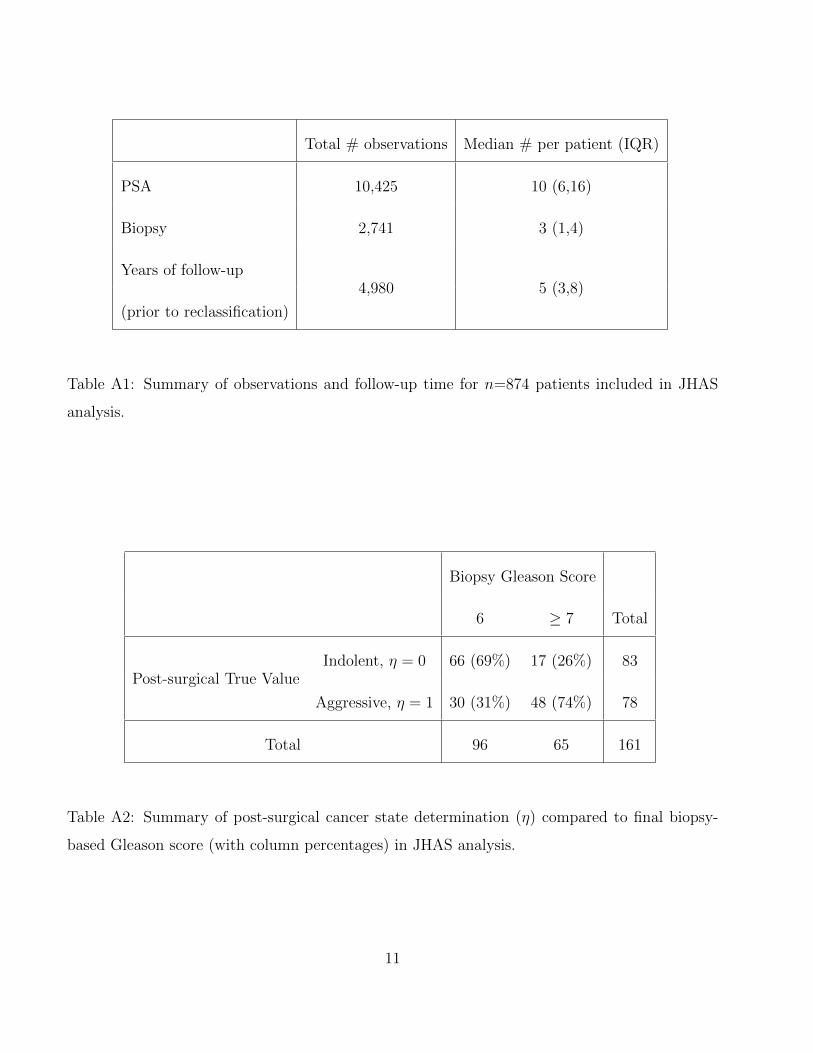
Total # observations Median # per patient (IQR)
PSA 10,425 10 (6,16)
Biopsy 2,741 3 (1,4)
Years of follow-up4,980 5 (3,8)
(prior to reclassification)
Table A1: Summary of observations and follow-up time for n=874 patients included in JHAS
analysis.
Biopsy Gleason Score
6 ≥ 7 Total
Post-surgical True ValueIndolent, η = 0 66 (69%) 17 (26%) 83
Aggressive, η = 1 30 (31%) 48 (74%) 78
Total 96 65 161
Table A2: Summary of post-surgical cancer state determination (η) compared to final biopsy-
based Gleason score (with column percentages) in JHAS analysis.
11
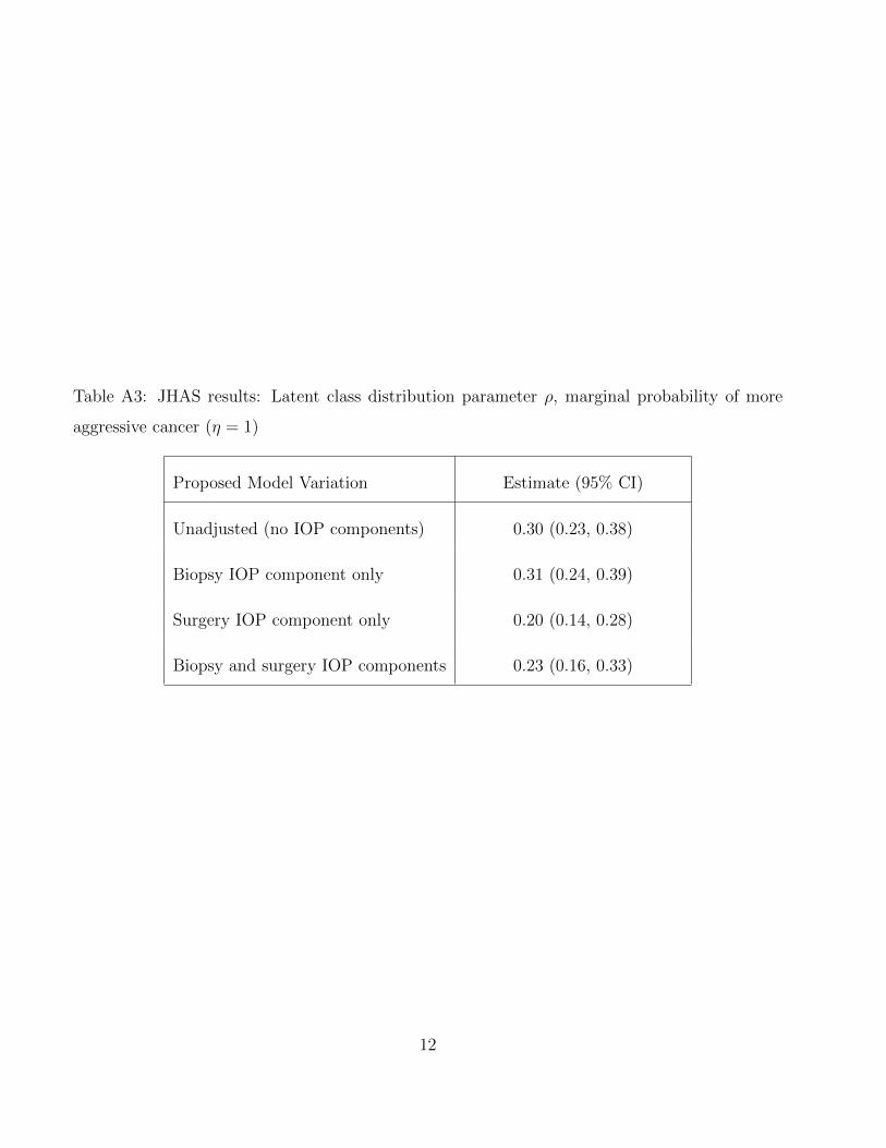
Table A3: JHAS results: Latent class distribution parameter ρ, marginal probability of more
aggressive cancer (η = 1)
Proposed Model Variation Estimate (95% CI)
Unadjusted (no IOP components) 0.30 (0.23, 0.38)
Biopsy IOP component only 0.31 (0.24, 0.39)
Surgery IOP component only 0.20 (0.14, 0.28)
Biopsy and surgery IOP components 0.23 (0.16, 0.33)
12
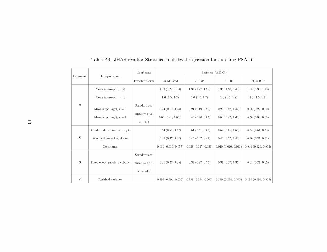
Table A4: JHAS results: Stratified multilevel regression for outcome PSA, Y
Parameter InterpretationCoefficient Estimate (95% CI)
Transformation Unadjusted B IOP S IOP B, S IOP
µ
Mean intercept, η = 0 1.33 (1.27, 1.38) 1.33 (1.27, 1.38) 1.36 (1.30, 1.40) 1.35 (1.30, 1.40)
Mean intercept, η = 1 1.6 (1.5, 1.7) 1.6 (1.5, 1.7) 1.6 (1.5, 1.8) 1.6 (1.5, 1.7)
Mean slope (age), η = 0Standardized
0.24 (0.19, 0.28) 0.24 (0.19, 0.29) 0.26 (0.22, 0.42) 0.26 (0.22, 0.30)
Mean slope (age), η = 1mean = 67.1
0.50 (0.41, 0.58) 0.48 (0.40, 0.57) 0.53 (0.42, 0.63) 0.50 (0.39, 0.60)
sd= 6.8
Σ
Standard deviation, intercepts 0.54 (0.51, 0.57) 0.54 (0.51, 0.57) 0.54 (0.51, 0.58) 0.54 (0.51, 0.58)
Standard deviation, slopes 0.39 (0.37, 0.42) 0.40 (0.37, 0.43) 0.40 (0.37, 0.43) 0.40 (0.37, 0.43)
Covariance 0.036 (0.016, 0.057) 0.038 (0.017, 0.059) 0.040 (0.020, 0.061) 0.041 (0.020, 0.063)
β Fixed effect, prostate volume
Standardized
0.31 (0.27, 0.35) 0.31 (0.27, 0.35) 0.31 (0.27, 0.35) 0.31 (0.27, 0.35)mean = 57.5
sd = 24.9
σ2 Residual variance 0.299 (0.294, 0.303) 0.299 (0.294, 0.303) 0.299 (0.294, 0.303) 0.299 (0.294, 0.303)
13
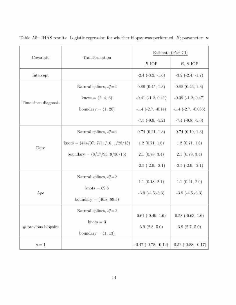
Table A5: JHAS results: Logistic regression for whether biopsy was performed, B; parameter: ν
Covariate TransformationEstimate (95% CI)
B IOP B, S IOP
Intercept -2.4 (-3.2, -1.6) -3.2 (-2.4, -1.7)
Time since diagnosis
Natural splines, df=4 0.86 (0.45, 1.3) 0.88 (0.46, 1.3)
knots = (2, 4, 6) -0.41 (-1.2, 0.41) -0.39 (-1.2, 0.47)
boundary = (1, 20) -1.4 (-2.7, -0.14) -1.4 (-2.7, -0.036)
-7.5 (-9.9, -5.2) -7.4 (-9.8, -5.0)
Date
Natural splines, df=4 0.74 (0.21, 1.3) 0.74 (0.19, 1.3)
knots = (4/4/07, 7/11/10, 1/28/13) 1.2 (0.71, 1.6) 1.2 (0.71, 1.6)
boundary = (8/17/95, 9/30/15) 2.1 (0.78, 3.4) 2.1 (0.79, 3.4)
-2.5 (-2.9, -2.1) -2.5 (-2.9, -2.1)
Age
Natural splines, df=21.1 (0.18, 2.1) 1.1 (0.21, 2.0)
knots = 69.8-3.9 (-4.5,-3.3) -3.9 (-4.5,-3.3)
boundary = (46.8, 89.5)
# previous biopsies
Natural splines, df=20.61 (-0.49, 1.6) 0.58 (-0.63, 1.6)
knots = 33.9 (2.8, 5.0) 3.9 (2.7, 5.0)
boundary = (1, 13)
η = 1 -0.47 (-0.78, -0.12) -0.52 (-0.88, -0.17)
14
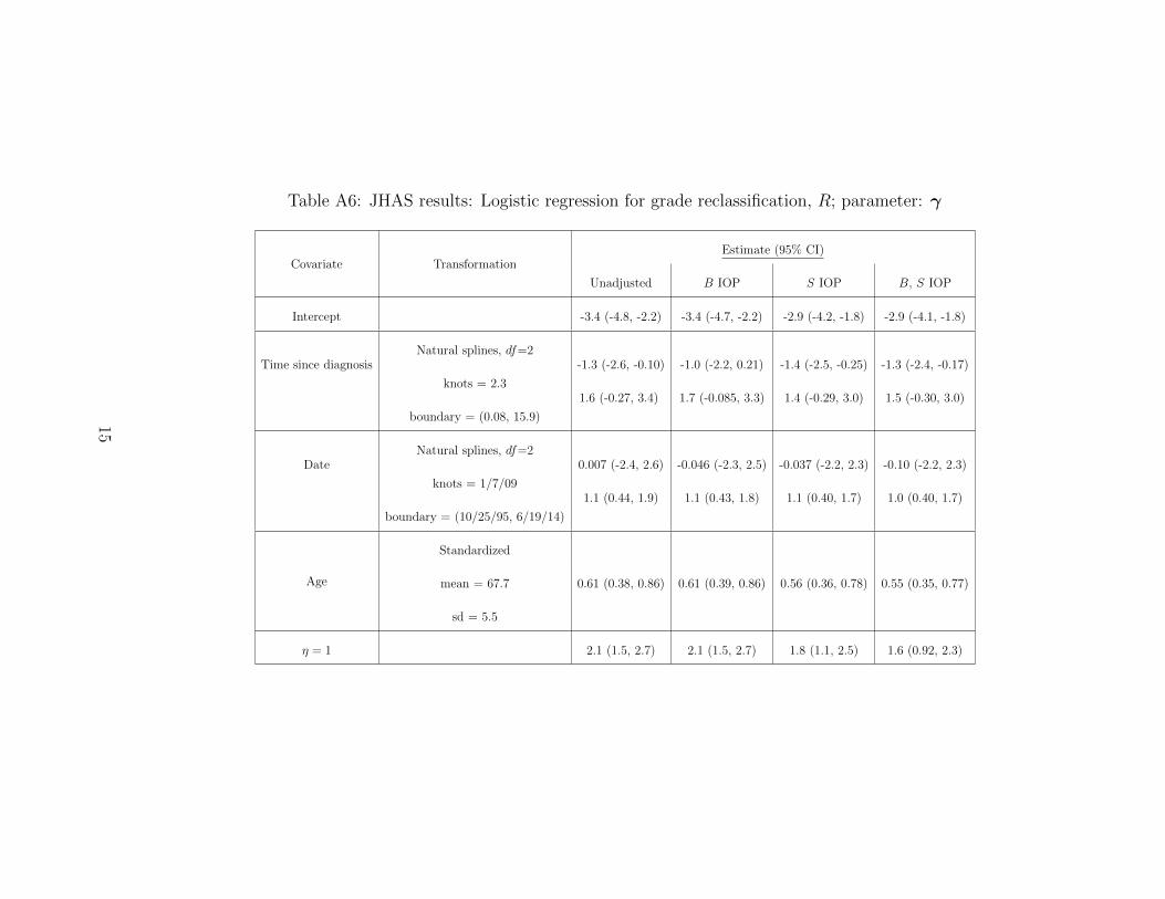
Table A6: JHAS results: Logistic regression for grade reclassification, R; parameter: γ
Covariate TransformationEstimate (95% CI)
Unadjusted B IOP S IOP B, S IOP
Intercept -3.4 (-4.8, -2.2) -3.4 (-4.7, -2.2) -2.9 (-4.2, -1.8) -2.9 (-4.1, -1.8)
Time since diagnosisNatural splines, df=2
-1.3 (-2.6, -0.10) -1.0 (-2.2, 0.21) -1.4 (-2.5, -0.25) -1.3 (-2.4, -0.17)
knots = 2.31.6 (-0.27, 3.4) 1.7 (-0.085, 3.3) 1.4 (-0.29, 3.0) 1.5 (-0.30, 3.0)
boundary = (0.08, 15.9)
DateNatural splines, df=2
0.007 (-2.4, 2.6) -0.046 (-2.3, 2.5) -0.037 (-2.2, 2.3) -0.10 (-2.2, 2.3)
knots = 1/7/091.1 (0.44, 1.9) 1.1 (0.43, 1.8) 1.1 (0.40, 1.7) 1.0 (0.40, 1.7)
boundary = (10/25/95, 6/19/14)
Age
Standardized
mean = 67.7 0.61 (0.38, 0.86) 0.61 (0.39, 0.86) 0.56 (0.36, 0.78) 0.55 (0.35, 0.77)
sd = 5.5
η = 1 2.1 (1.5, 2.7) 2.1 (1.5, 2.7) 1.8 (1.1, 2.5) 1.6 (0.92, 2.3)
15
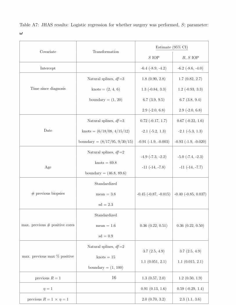
Table A7: JHAS results: Logistic regression for whether surgery was performed, S; parameter:
ω
Covariate TransformationEstimate (95% CI)
S IOP B, S IOP
Intercept -6.4 (-8.9, -4.2) -6.2 (-8.6, -4.0)
Time since diagnosis
Natural splines, df=3 1.8 (0.90, 2.8) 1.7 (0.82, 2.7)
knots = (2, 4, 6) 1.3 (-0.84, 3.3) 1.2 (-0.93, 3.3)
boundary = (1, 20) 6.7 (3.9, 9.5) 6.7 (3.8, 9.4)
2.9 (-2.0, 6.8) 2.9 (-2.0, 6.8)
Date
Natural splines, df=3 0.72 (-0.17, 1.7) 0.67 (-0.22, 1.6)
knots = (6/18/08, 4/15/12) -2.1 (-5.2, 1.3) -2.1 (-5.3, 1.3)
boundary = (8/17/95, 9/30/15) -0.91 (-1.9, -0.003) -0.93 (-1.9, -0.020)
Age
Natural splines, df=2-4.9 (-7.3, -2.2) -5.0 (-7.4, -2.3)
knots = 69.8-11 (-14, -7.8) -11 (-14, -7.7)
boundary = (46.8, 89.6)
# previous biopsies
Standardized
mean = 3.8 -0.45 (-0.87, -0.015) -0.40 (-0.85, 0.037)
sd = 2.3
max. previous # positive cores
Standardized
mean = 1.6 0.36 (0.22, 0.51) 0.36 (0.22, 0.50)
sd = 0.9
max. previous max % positive
Natural splines, df=23.7 (2.5, 4.9) 3.7 (2.5, 4.9)
knots = 151.1 (0.051, 2.1) 1.1 (0.015, 2.1)
boundary = (1, 100)
previous R = 1 1.3 (0.57, 2.0) 1.2 (0.50, 1.9)
η = 1 0.91 (0.13, 1.6) 0.59 (-0.29, 1.4)
previous R = 1 × η = 1 2.0 (0.70, 3.2) 2.3 (1.1, 3.6)
16
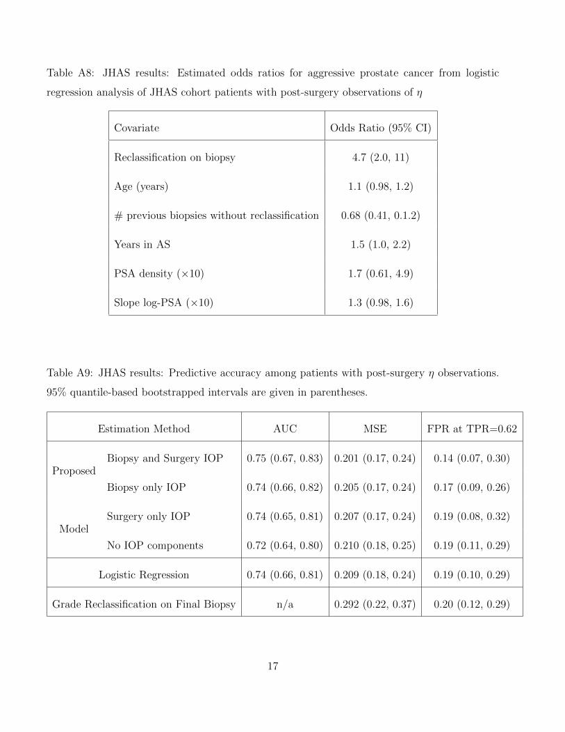
Table A8: JHAS results: Estimated odds ratios for aggressive prostate cancer from logistic
regression analysis of JHAS cohort patients with post-surgery observations of η
Covariate Odds Ratio (95% CI)
Reclassification on biopsy 4.7 (2.0, 11)
Age (years) 1.1 (0.98, 1.2)
# previous biopsies without reclassification 0.68 (0.41, 0.1.2)
Years in AS 1.5 (1.0, 2.2)
PSA density (×10) 1.7 (0.61, 4.9)
Slope log-PSA (×10) 1.3 (0.98, 1.6)
Table A9: JHAS results: Predictive accuracy among patients with post-surgery η observations.
95% quantile-based bootstrapped intervals are given in parentheses.
Estimation Method AUC MSE FPR at TPR=0.62
ProposedBiopsy and Surgery IOP 0.75 (0.67, 0.83) 0.201 (0.17, 0.24) 0.14 (0.07, 0.30)
Biopsy only IOP 0.74 (0.66, 0.82) 0.205 (0.17, 0.24) 0.17 (0.09, 0.26)
ModelSurgery only IOP 0.74 (0.65, 0.81) 0.207 (0.17, 0.24) 0.19 (0.08, 0.32)
No IOP components 0.72 (0.64, 0.80) 0.210 (0.18, 0.25) 0.19 (0.11, 0.29)
Logistic Regression 0.74 (0.66, 0.81) 0.209 (0.18, 0.24) 0.19 (0.10, 0.29)
Grade Reclassification on Final Biopsy n/a 0.292 (0.22, 0.37) 0.20 (0.12, 0.29)
17
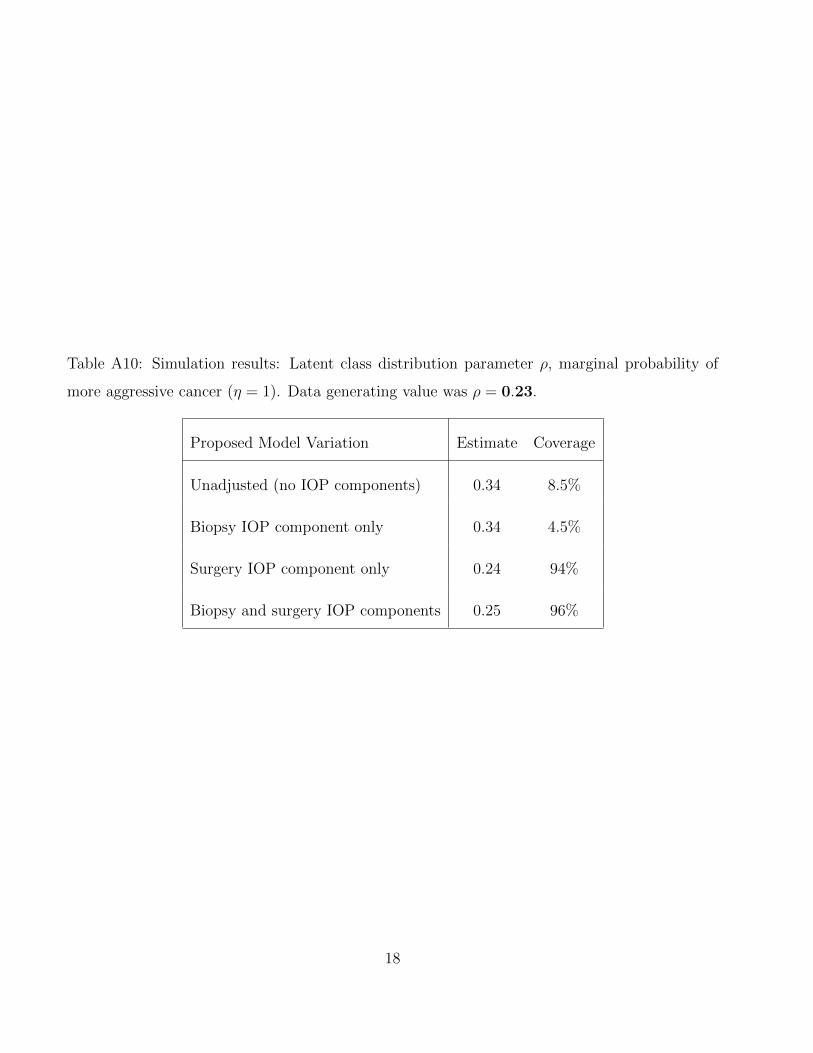
Table A10: Simulation results: Latent class distribution parameter ρ, marginal probability of
more aggressive cancer (η = 1). Data generating value was ρ = 0.23.
Proposed Model Variation Estimate Coverage
Unadjusted (no IOP components) 0.34 8.5%
Biopsy IOP component only 0.34 4.5%
Surgery IOP component only 0.24 94%
Biopsy and surgery IOP components 0.25 96%
18
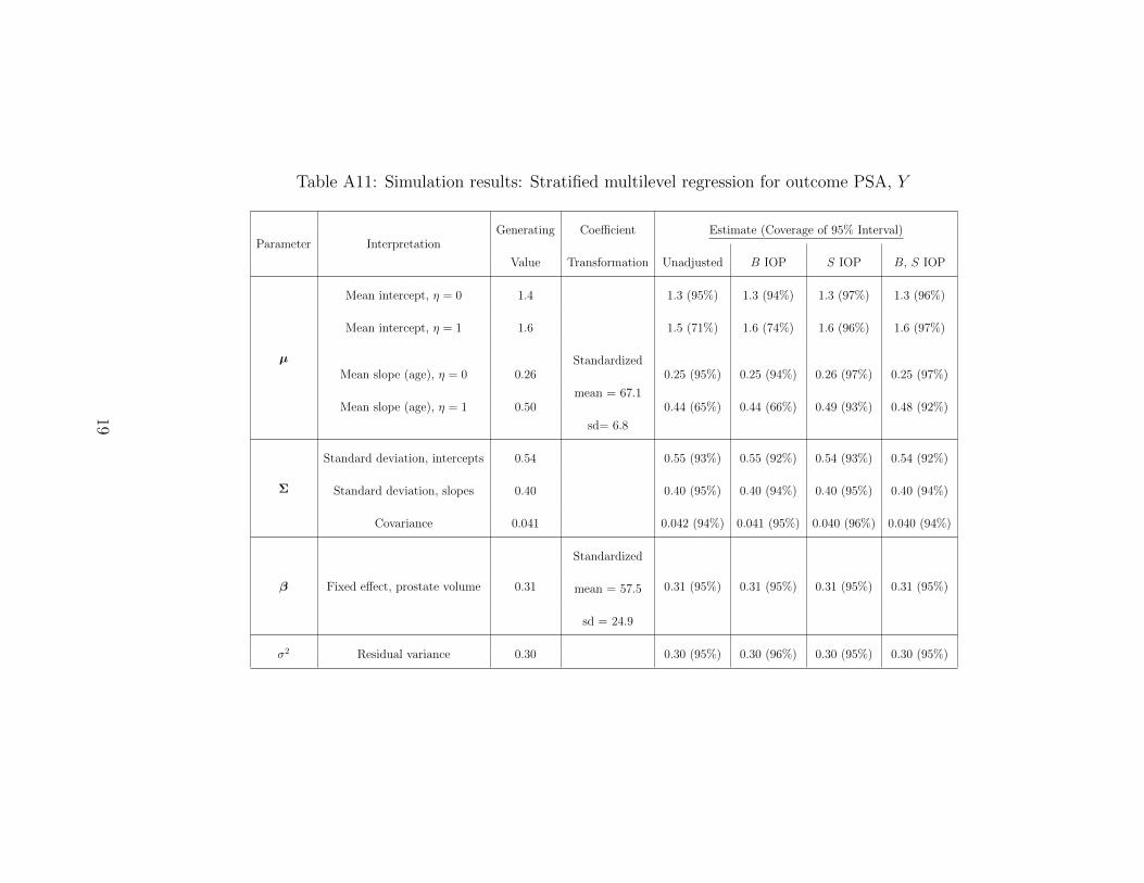
Table A11: Simulation results: Stratified multilevel regression for outcome PSA, Y
Parameter InterpretationGenerating Coefficient Estimate (Coverage of 95% Interval)
Value Transformation Unadjusted B IOP S IOP B, S IOP
µ
Mean intercept, η = 0 1.4 1.3 (95%) 1.3 (94%) 1.3 (97%) 1.3 (96%)
Mean intercept, η = 1 1.6 1.5 (71%) 1.6 (74%) 1.6 (96%) 1.6 (97%)
Mean slope (age), η = 0 0.26Standardized
0.25 (95%) 0.25 (94%) 0.26 (97%) 0.25 (97%)
Mean slope (age), η = 1 0.50mean = 67.1
0.44 (65%) 0.44 (66%) 0.49 (93%) 0.48 (92%)
sd= 6.8
Σ
Standard deviation, intercepts 0.54 0.55 (93%) 0.55 (92%) 0.54 (93%) 0.54 (92%)
Standard deviation, slopes 0.40 0.40 (95%) 0.40 (94%) 0.40 (95%) 0.40 (94%)
Covariance 0.041 0.042 (94%) 0.041 (95%) 0.040 (96%) 0.040 (94%)
β Fixed effect, prostate volume 0.31
Standardized
0.31 (95%) 0.31 (95%) 0.31 (95%) 0.31 (95%)mean = 57.5
sd = 24.9
σ2 Residual variance 0.30 0.30 (95%) 0.30 (96%) 0.30 (95%) 0.30 (95%)
19
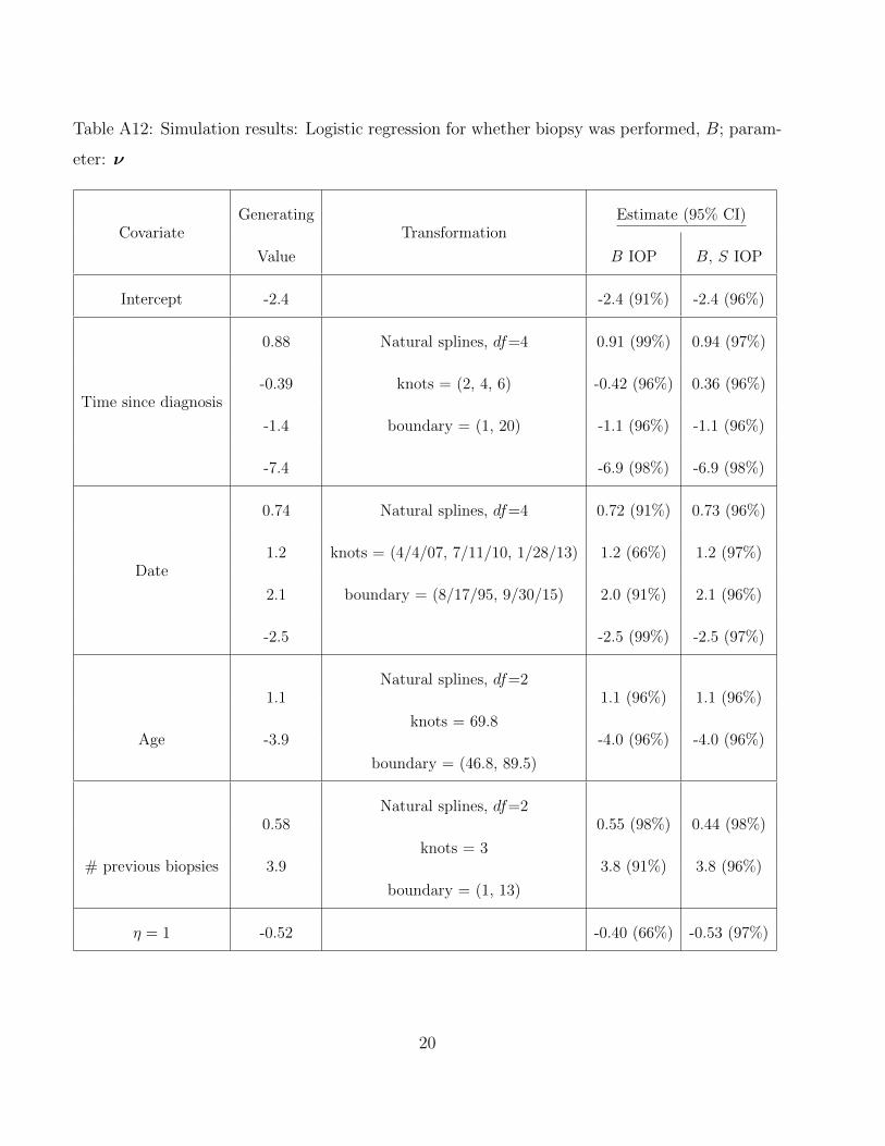
Table A12: Simulation results: Logistic regression for whether biopsy was performed, B; param-
eter: ν
CovariateGenerating
TransformationEstimate (95% CI)
Value B IOP B, S IOP
Intercept -2.4 -2.4 (91%) -2.4 (96%)
Time since diagnosis
0.88 Natural splines, df=4 0.91 (99%) 0.94 (97%)
-0.39 knots = (2, 4, 6) -0.42 (96%) 0.36 (96%)
-1.4 boundary = (1, 20) -1.1 (96%) -1.1 (96%)
-7.4 -6.9 (98%) -6.9 (98%)
Date
0.74 Natural splines, df=4 0.72 (91%) 0.73 (96%)
1.2 knots = (4/4/07, 7/11/10, 1/28/13) 1.2 (66%) 1.2 (97%)
2.1 boundary = (8/17/95, 9/30/15) 2.0 (91%) 2.1 (96%)
-2.5 -2.5 (99%) -2.5 (97%)
Age
1.1Natural splines, df=2
1.1 (96%) 1.1 (96%)
-3.9knots = 69.8
-4.0 (96%) -4.0 (96%)
boundary = (46.8, 89.5)
# previous biopsies
0.58Natural splines, df=2
0.55 (98%) 0.44 (98%)
3.9knots = 3
3.8 (91%) 3.8 (96%)
boundary = (1, 13)
η = 1 -0.52 -0.40 (66%) -0.53 (97%)
20
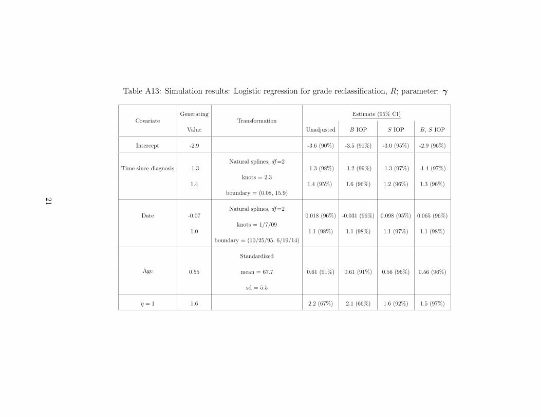
Table A13: Simulation results: Logistic regression for grade reclassification, R; parameter: γ
CovariateGenerating
TransformationEstimate (95% CI)
Value Unadjusted B IOP S IOP B, S IOP
Intercept -2.9 -3.6 (90%) -3.5 (91%) -3.0 (95%) -2.9 (96%)
Time since diagnosis -1.3Natural splines, df=2
-1.3 (98%) -1.2 (99%) -1.3 (97%) -1.4 (97%)
1.4knots = 2.3
1.4 (95%) 1.6 (96%) 1.2 (96%) 1.3 (96%)
boundary = (0.08, 15.9)
Date -0.07Natural splines, df=2
0.018 (96%) -0.031 (96%) 0.098 (95%) 0.065 (96%)
1.0knots = 1/7/09
1.1 (98%) 1.1 (98%) 1.1 (97%) 1.1 (98%)
boundary = (10/25/95, 6/19/14)
Age
Standardized
0.55 mean = 67.7 0.61 (91%) 0.61 (91%) 0.56 (96%) 0.56 (96%)
sd = 5.5
η = 1 1.6 2.2 (67%) 2.1 (66%) 1.6 (92%) 1.5 (97%)
21
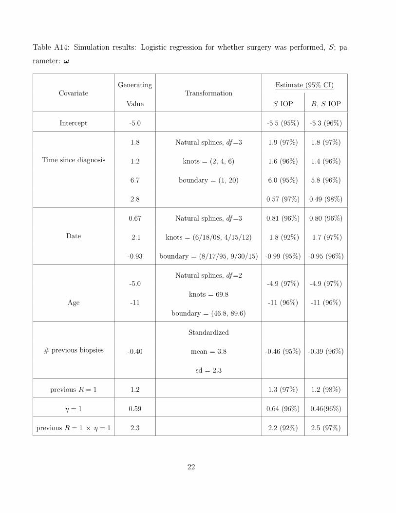
Table A14: Simulation results: Logistic regression for whether surgery was performed, S; pa-
rameter: ω
CovariateGenerating
TransformationEstimate (95% CI)
Value S IOP B, S IOP
Intercept -5.0 -5.5 (95%) -5.3 (96%)
Time since diagnosis
1.8 Natural splines, df=3 1.9 (97%) 1.8 (97%)
1.2 knots = (2, 4, 6) 1.6 (96%) 1.4 (96%)
6.7 boundary = (1, 20) 6.0 (95%) 5.8 (96%)
2.8 0.57 (97%) 0.49 (98%)
Date
0.67 Natural splines, df=3 0.81 (96%) 0.80 (96%)
-2.1 knots = (6/18/08, 4/15/12) -1.8 (92%) -1.7 (97%)
-0.93 boundary = (8/17/95, 9/30/15) -0.99 (95%) -0.95 (96%)
Age
-5.0Natural splines, df=2
-4.9 (97%) -4.9 (97%)
-11knots = 69.8
-11 (96%) -11 (96%)
boundary = (46.8, 89.6)
# previous biopsies
Standardized
-0.40 mean = 3.8 -0.46 (95%) -0.39 (96%)
sd = 2.3
previous R = 1 1.2 1.3 (97%) 1.2 (98%)
η = 1 0.59 0.64 (96%) 0.46(96%)
previous R = 1 × η = 1 2.3 2.2 (92%) 2.5 (97%)
22
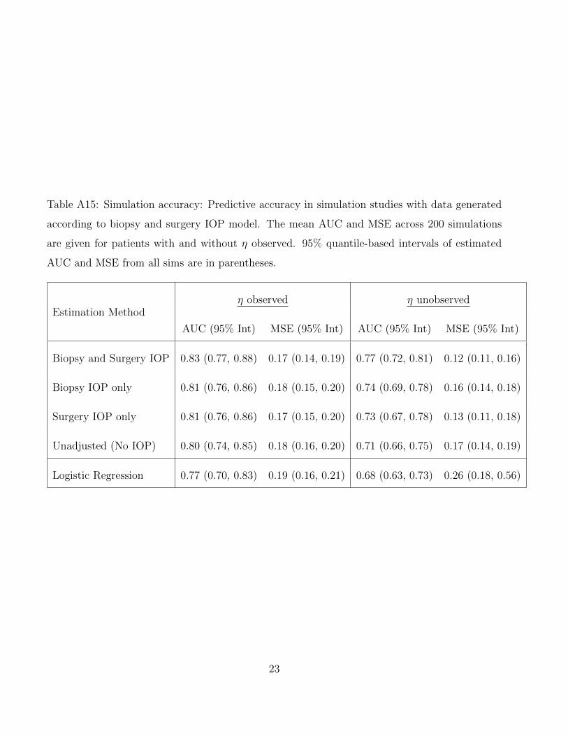
Table A15: Simulation accuracy: Predictive accuracy in simulation studies with data generated
according to biopsy and surgery IOP model. The mean AUC and MSE across 200 simulations
are given for patients with and without η observed. 95% quantile-based intervals of estimated
AUC and MSE from all sims are in parentheses.
Estimation Methodη observed η unobserved
AUC (95% Int) MSE (95% Int) AUC (95% Int) MSE (95% Int)
Biopsy and Surgery IOP 0.83 (0.77, 0.88) 0.17 (0.14, 0.19) 0.77 (0.72, 0.81) 0.12 (0.11, 0.16)
Biopsy IOP only 0.81 (0.76, 0.86) 0.18 (0.15, 0.20) 0.74 (0.69, 0.78) 0.16 (0.14, 0.18)
Surgery IOP only 0.81 (0.76, 0.86) 0.17 (0.15, 0.20) 0.73 (0.67, 0.78) 0.13 (0.11, 0.18)
Unadjusted (No IOP) 0.80 (0.74, 0.85) 0.18 (0.16, 0.20) 0.71 (0.66, 0.75) 0.17 (0.14, 0.19)
Logistic Regression 0.77 (0.70, 0.83) 0.19 (0.16, 0.21) 0.68 (0.63, 0.73) 0.26 (0.18, 0.56)
23
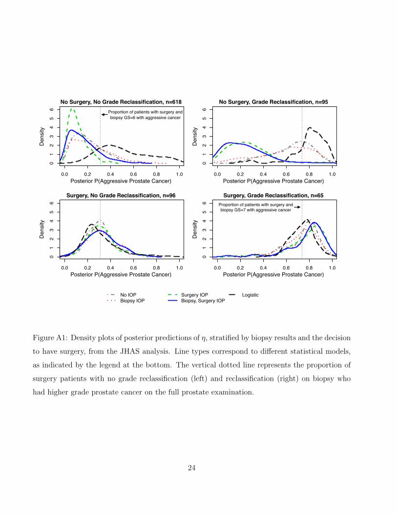
0.0 0.2 0.4 0.6 0.8 1.0
01
23
45
6
0.0 0.2 0.4 0.6 0.8 1.0
01
23
45
6
0.0 0.2 0.4 0.6 0.8 1.0
01
23
45
6
0.0 0.2 0.4 0.6 0.8 1.0
01
23
45
6
No IOPBiopsy IOP
Surgery IOPBiopsy, Surgery IOP
Logistic
Posterior P(Aggressive Prostate Cancer)
Posterior P(Aggressive Prostate Cancer) Posterior P(Aggressive Prostate Cancer)
Posterior P(Aggressive Prostate Cancer)
Den
sity
Den
sity
Den
sity
Den
sity
No Surgery, No Grade Reclassification, n=618
Surgery, No Grade Reclassification, n=96
No Surgery, Grade Reclassification, n=95
Surgery, Grade Reclassification, n=65
Proportion of patients with surgery and biopsy GS=6 with aggressive cancer
Proportion of patients with surgery and biopsy GS=7 with aggressive cancer
Figure A1: Density plots of posterior predictions of η, stratified by biopsy results and the decision
to have surgery, from the JHAS analysis. Line types correspond to different statistical models,
as indicated by the legend at the bottom. The vertical dotted line represents the proportion of
surgery patients with no grade reclassification (left) and reclassification (right) on biopsy who
had higher grade prostate cancer on the full prostate examination.
24
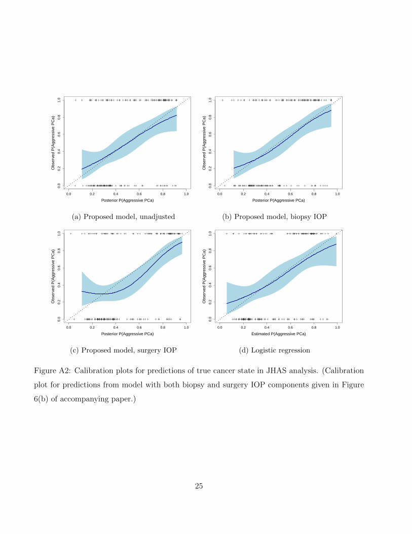
Posterior P(Aggressive PCa)
Obs
erve
d P
(Agg
ress
ive
PC
a)
0.0 0.2 0.4 0.6 0.8 1.0
0.0
0.2
0.4
0.6
0.8
1.0
(a) Proposed model, unadjusted
Posterior P(Aggressive PCa)O
bser
ved
P(A
ggre
ssiv
e P
Ca)
0.0 0.2 0.4 0.6 0.8 1.0
0.0
0.2
0.4
0.6
0.8
1.0
(b) Proposed model, biopsy IOP
Posterior P(Aggressive PCa)
Obs
erve
d P
(Agg
ress
ive
PC
a)
0.0 0.2 0.4 0.6 0.8 1.0
0.0
0.2
0.4
0.6
0.8
1.0
(c) Proposed model, surgery IOP
Estimated P(Aggressive PCa)
Obs
erve
d P
(Agg
ress
ive
PC
a)
0.0 0.2 0.4 0.6 0.8 1.0
0.0
0.2
0.4
0.6
0.8
1.0
(d) Logistic regression
Figure A2: Calibration plots for predictions of true cancer state in JHAS analysis. (Calibration
plot for predictions from model with both biopsy and surgery IOP components given in Figure
6(b) of accompanying paper.)
25
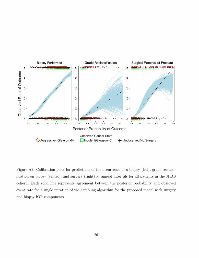
Obs
erve
d R
ate
of O
utco
me
Posterior Probability of Outcome
Observed Cancer State Aggressive (Gleason>6) Indolent(Gleason=6) Unobserved/No Surgery
Figure A3: Calibration plots for predictions of the occurrence of a biopsy (left), grade reclassi-
fication on biopsy (center), and surgery (right) at annual intervals for all patients in the JHAS
cohort. Each solid line represents agreement between the posterior probability and observed
event rate for a single iteration of the sampling algorithm for the proposed model with surgery
and biopsy IOP components.
26
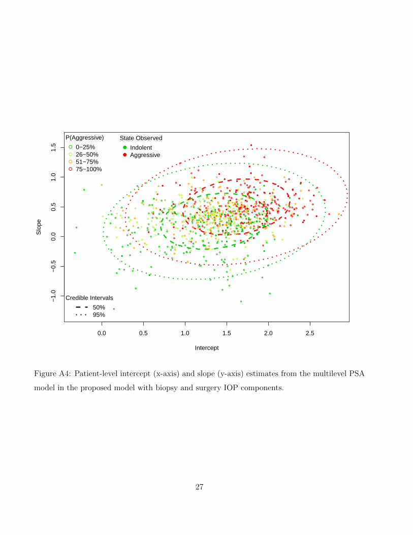
0.0 0.5 1.0 1.5 2.0 2.5
−1.
0−
0.5
0.0
0.5
1.0
1.5
Intercept
Slo
pe
●
●
●
●●
●
●
●
●
●
●
●
●
●
●
●
●
●
●
●
●
●
●
●
●
●
●
●
●
●
●
●
●
●
●
●
●
●
●
●
●
●
●
●
●
●
●
●
●
●
●
●●
●
●
●
●
●
●
●
●●
●
●●
●
●
●
●
●
●
●
●
●
●
●
●
●
●
●●
●
●
●
●
●
●
●
●●
●
●
●
●
●
●
●
● ●
●
●
●
●
●
●
●
●
●
●
●
●
●
●
●
●
●
●
●
●
●●
●
●
●
●
●
●
●
●
●
●
●
●
●
●
●
●
●
●
●
●
●
●
●
●
●
●
●
●●
●
●
●
●
●
●
●
●
●●
●
●
●
●
●
●
●
●
●
●
●
●
●
●
●
●
●
●
●
●
●
●
●
●
●
●
●
●
●
●
●
●
●
●
●
●
●
●
●
●
●
●
●
●
●
●
●
●
●
●
●
●
●
●
●
●
●
●
●
●
●
●
●
●
●
●
●
●
●
●
●
●
●
●
●
●
●
●
●
●
●
●
●
●
●
●
●
●
●
●
●
●
●
●
●
●
●
●
●
●
●
●
●●
●
●
●
●
●
●
●
● ●
●
●
●
●
●
●
●
●
● ●
●
●
●●
●
●
●
●
●
●
●
●
●
●
●
●
●
●
●●
●
●
●
●
●
●
●
●
●
●
●
●
●
●
●
●
●
●
●
●
●
●
●
● ●
●
●
●
●
●
●
●
●
●
●
●
●
●
●
●
●
●
●
●
●●
●
●
●
●
●
●
●
●
●
●
●
●
●
●
●
●
●
●
●●
●●
●
●
●
●
●
●
●
●
●
●
●
●
●
●
●
● ●
●
●
●
●
●●
●
●
●
●
●
●
●
●
●
●
●
●
●
●
●
●
●
●
●
●
●
●
●
●
●
●
●
●
●
●
●
●
●
●
●
●
●
●
●
●
●
●
●
●
●
●
●
●
●
●
●
●
●
●
●
●
●
●
●
●
●
●
●
●
●
●
●
●
●
●
●
●
●
●
●
●
●
●
●
●
●
●
●
●
●
●
●
●●
● ●
●
●
●
●
●
●
●
●
●
●
●
●
●
●
●
●
●
●
●
●
●
●
●
●●
●
●
●
●
●
●
●
●
●
●
●
●
●
● ●
●
●●
●
●
●
●
●
●
●
●
●
●
●
●
●
●
●
●
●
●
●
●
●
●
●
●
●
●
●
●
●
●
●
●
●
●
●
●●
●
●
●
●
●
●
●
●
●●
●
●
●
●
●
●
●
●
●
●
●
●
●
● ●
●
●
●
●
●
●
●
●
●
●
●
●
●
●
●
●
●
●
●
●
●
●
●
●
●
●
●
●
●
●●
●
●
●
●
●
●
●
●
●
●
●
●
●
● ●
●
●
●
●
●
●
●
●
●
●
●
●
●
●
●
●
●
●
●
●
●
●
●
●
●
●
●
●
●
●
●●
●
●
●
●
●
●
●
●
●
●
●
●
●
●
●
●
●
●
●
●
●
●
●
●
●
●
●
●
●
●
●
●
●
●
●
●
●
●
●
●
●
●
●
●
●
●
●
●●
●
●
●
●
●
●
●
●
●
●
●
●
●
●
●
●
●
●
●
●
●
●
●
●
●
●
●
●
●
●
●
●
●
●●
●
●
●
●
●
●
●
●
●
●
● ●
●
●
●
●
●
●
●
●
●
●
●
●
●
●
●
●
●
●
●
●
●
●
●
●
●
●
●
●
●●
●
●
●
●
●
●
●
●
●
●
●
●
●
●
●
●
●
●
●
● ●
●
●
●
●
●
●
●
●
●
●
●●
●
●
●
●
●
●
●
●
●
●
●
●
●
●
●
●
●
●
●
●
●
●
●
●
●●
●
●
●
● ●
●
●
●
●
●
●
●
●
●
●
●
●
●
●
●
●
●
●
●
●
P(Aggressive)
0−25%26−50%51−75%75−100%
●
●
State Observed
IndolentAggressive
Credible Intervals
50%95%
Figure A4: Patient-level intercept (x-axis) and slope (y-axis) estimates from the multilevel PSA
model in the proposed model with biopsy and surgery IOP components.
27
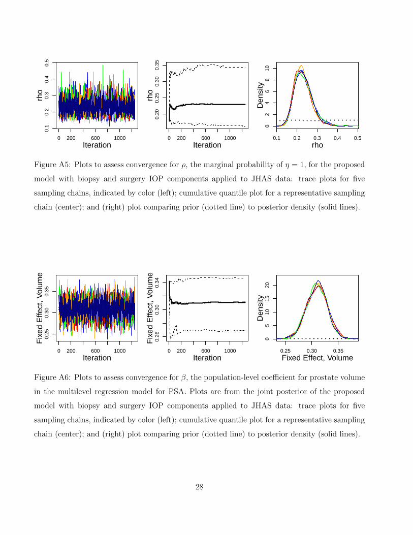
0 200 600 1000
0.1
0.2
0.3
0.4
0.5
Iteration
rho
0 200 600 1000
0.20
0.25
0.30
0.35
Iterationrh
o
0.1 0.2 0.3 0.4 0.5
02
46
810
Den
sity
rho
Figure A5: Plots to assess convergence for ρ, the marginal probability of η = 1, for the proposed
model with biopsy and surgery IOP components applied to JHAS data: trace plots for five
sampling chains, indicated by color (left); cumulative quantile plot for a representative sampling
chain (center); and (right) plot comparing prior (dotted line) to posterior density (solid lines).
0 200 600 1000
0.25
0.30
0.35
Iteration
Fix
ed E
ffect
, Vol
ume
0 200 600 1000
0.26
0.30
0.34
Iteration
Fix
ed E
ffect
, Vol
ume
0.25 0.30 0.35
05
1015
20D
ensi
ty
Fixed Effect, Volume
Figure A6: Plots to assess convergence for β, the population-level coefficient for prostate volume
in the multilevel regression model for PSA. Plots are from the joint posterior of the proposed
model with biopsy and surgery IOP components applied to JHAS data: trace plots for five
sampling chains, indicated by color (left); cumulative quantile plot for a representative sampling
chain (center); and (right) plot comparing prior (dotted line) to posterior density (solid lines).
28
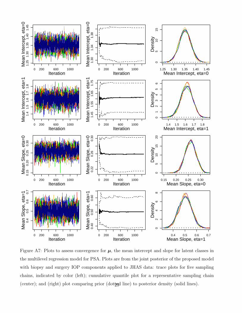
0 200 600 1000
1.25
1.30
1.35
1.40
1.45
Iteration
Mea
n In
terc
ept,
eta=
0
0 200 600 1000
1.30
1.34
1.38
Iteration
Mea
n In
terc
ept,
eta=
0
1.25 1.30 1.35 1.40 1.45
05
1015
Den
sity
Mean Intercept, eta=0
0 200 600 1000
1.4
1.5
1.6
1.7
1.8
Iteration
Mea
n In
terc
ept,
eta=
1
0 200 600 1000
1.45
1.55
1.65
1.75
Iteration
Mea
n In
terc
ept,
eta=
1
1.4 1.5 1.6 1.7 1.8
01
23
45
6D
ensi
ty
Mean Intercept, eta=1
0 200 600 1000
0.15
0.20
0.25
0.30
Iteration
Mea
n S
lope
, eta
=0
0 200 600 1000
0.22
0.26
0.30
Iteration
Mea
n S
lope
, eta
=0
0.15 0.20 0.25 0.30
05
1015
20D
ensi
ty
Mean Slope, eta=0
0 200 600 1000
0.4
0.5
0.6
0.7
Iteration
Mea
n S
lope
, eta
=1
0 200 600 1000
0.40
0.50
0.60
Iteration
Mea
n S
lope
, eta
=1
0.4 0.5 0.6 0.7
02
46
8D
ensi
ty
Mean Slope, eta=1
Figure A7: Plots to assess convergence for µ, the mean intercept and slope for latent classes in
the multilevel regression model for PSA. Plots are from the joint posterior of the proposed model
with biopsy and surgery IOP components applied to JHAS data: trace plots for five sampling
chains, indicated by color (left); cumulative quantile plot for a representative sampling chain
(center); and (right) plot comparing prior (dotted line) to posterior density (solid lines).29
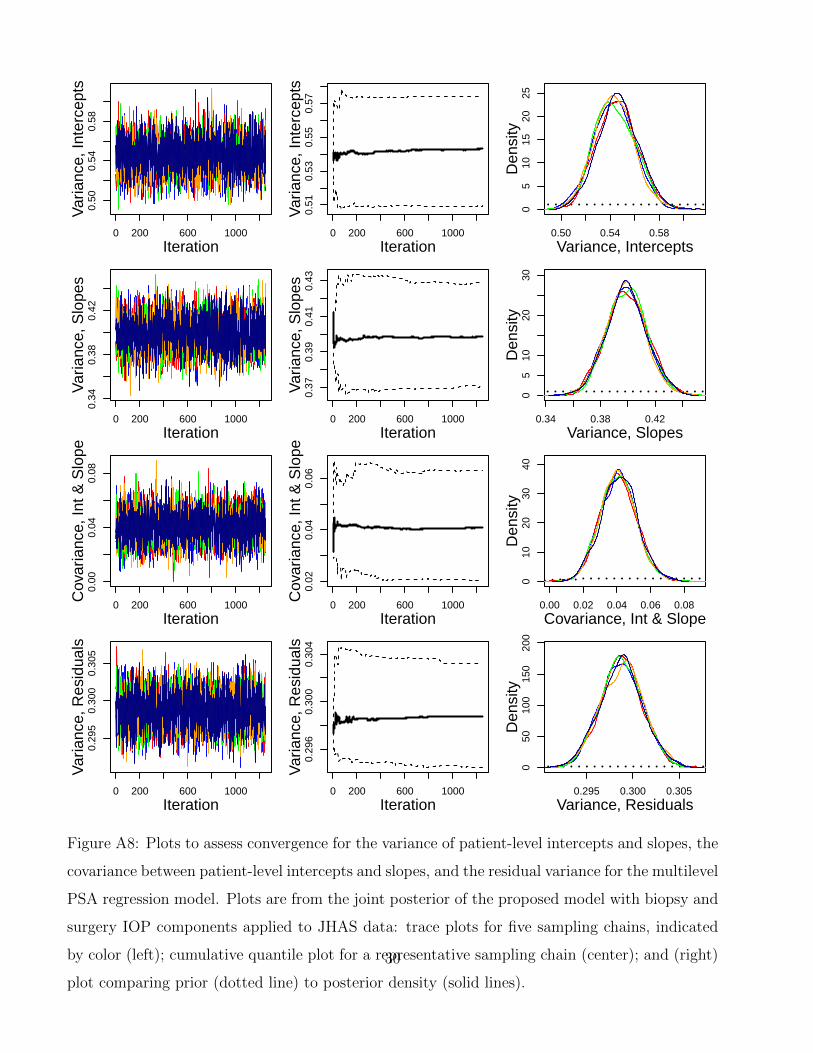
0 200 600 1000
0.50
0.54
0.58
Iteration
Var
ianc
e, In
terc
epts
0 200 600 1000
0.51
0.53
0.55
0.57
Iteration
Var
ianc
e, In
terc
epts
0.50 0.54 0.58
05
1015
2025
Den
sity
Variance, Intercepts
0 200 600 1000
0.34
0.38
0.42
Iteration
Var
ianc
e, S
lope
s
0 200 600 1000
0.37
0.39
0.41
0.43
Iteration
Var
ianc
e, S
lope
s
0.34 0.38 0.42
05
1020
30D
ensi
ty
Variance, Slopes
0 200 600 1000
0.00
0.04
0.08
Iteration
Cov
aria
nce,
Int &
Slo
pe
0 200 600 1000
0.02
0.04
0.06
Iteration
Cov
aria
nce,
Int &
Slo
pe
0.00 0.02 0.04 0.06 0.08
010
2030
40D
ensi
ty
Covariance, Int & Slope
0 200 600 1000
0.29
50.
300
0.30
5
Iteration
Var
ianc
e, R
esid
uals
0 200 600 1000
0.29
60.
300
0.30
4
Iteration
Var
ianc
e, R
esid
uals
0.295 0.300 0.305
050
100
150
200
Den
sity
Variance, Residuals
Figure A8: Plots to assess convergence for the variance of patient-level intercepts and slopes, the
covariance between patient-level intercepts and slopes, and the residual variance for the multilevel
PSA regression model. Plots are from the joint posterior of the proposed model with biopsy and
surgery IOP components applied to JHAS data: trace plots for five sampling chains, indicated
by color (left); cumulative quantile plot for a representative sampling chain (center); and (right)
plot comparing prior (dotted line) to posterior density (solid lines).
30
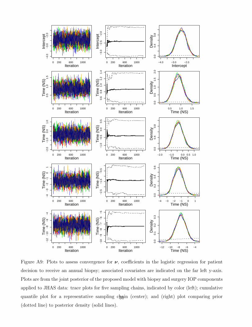
0 200 600 1000
−4.
0−
3.0
−2.
0
Iteration
Inte
rcep
t
0 200 600 1000
−3.
0−
2.5
−2.
0
Iteration
Inte
rcep
t
−4.0 −3.0 −2.0
0.0
0.4
0.8
Den
sity
Intercept
0 200 600 1000
0.5
1.0
1.5
Iteration
Tim
e (N
S)
0 200 600 1000
0.6
0.8
1.0
1.2
1.4
Iteration
Tim
e (N
S)
0.5 1.0 1.5
0.0
0.5
1.0
1.5
2.0
Den
sity
Time (NS)
0 200 600 1000
−2.
0−
1.0
0.0
1.0
Iteration
Tim
e (N
S)
0 200 600 1000
−1.
0−
0.5
0.0
0.5
Iteration
Tim
e (N
S)
−2.0 −1.0 0.0 0.5 1.00.
00.
40.
8D
ensi
ty
Time (NS)
0 200 600 1000
−4
−3
−2
−1
01
Iteration
Tim
e (N
S)
0 200 600 1000
−2.
5−
1.5
−0.
5
Iteration
Tim
e (N
S)
−4 −3 −2 −1 0 1
0.0
0.2
0.4
0.6
Den
sity
Time (NS)
0 200 600 1000
−12
−10
−8
−6
−4
Iteration
Tim
e (N
S)
0 200 600 1000
−10
−9
−8
−7
−6
−5
Iteration
Tim
e (N
S)
−12 −10 −8 −6 −4
0.0
0.1
0.2
0.3
Den
sity
Time (NS)
Figure A9: Plots to assess convergence for ν, coefficients in the logistic regression for patient
decision to receive an annual biopsy; associated covariates are indicated on the far left y-axis.
Plots are from the joint posterior of the proposed model with biopsy and surgery IOP components
applied to JHAS data: trace plots for five sampling chains, indicated by color (left); cumulative
quantile plot for a representative sampling chain (center); and (right) plot comparing prior
(dotted line) to posterior density (solid lines).
31
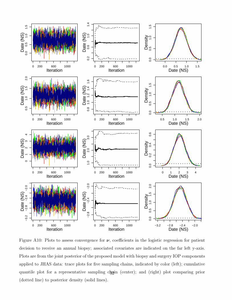
0 200 600 1000
0.0
0.5
1.0
1.5
Iteration
Dat
e (N
S)
0 200 600 1000
0.2
0.6
1.0
1.4
Iteration
Dat
e (N
S)
0.0 0.5 1.0 1.5
0.0
0.5
1.0
1.5
Den
sity
Date (NS)
0 200 600 1000
0.5
1.0
1.5
2.0
Iteration
Dat
e (N
S)
0 200 600 1000
0.8
1.0
1.2
1.4
1.6
Iteration
Dat
e (N
S)
0.5 1.0 1.5 2.0
0.0
0.5
1.0
1.5
Den
sity
Date (NS)
0 200 600 1000
01
23
4
Iteration
Dat
e (N
S)
0 200 600 1000
1.0
2.0
3.0
Iteration
Dat
e (N
S)
0 1 2 3 4
0.0
0.2
0.4
0.6
Den
sity
Date (NS)
0 200 600 1000
−3.
2−
2.8
−2.
4−
2.0
Iteration
Dat
e (N
S)
0 200 600 1000
−2.
8−
2.4
−2.
0
Iteration
Dat
e (N
S)
−3.2 −2.8 −2.4 −2.0
0.0
0.5
1.0
1.5
2.0
Den
sity
Date (NS)
Figure A10: Plots to assess convergence for ν, coefficients in the logistic regression for patient
decision to receive an annual biopsy; associated covariates are indicated on the far left y-axis.
Plots are from the joint posterior of the proposed model with biopsy and surgery IOP components
applied to JHAS data: trace plots for five sampling chains, indicated by color (left); cumulative
quantile plot for a representative sampling chain (center); and (right) plot comparing prior
(dotted line) to posterior density (solid lines).
32
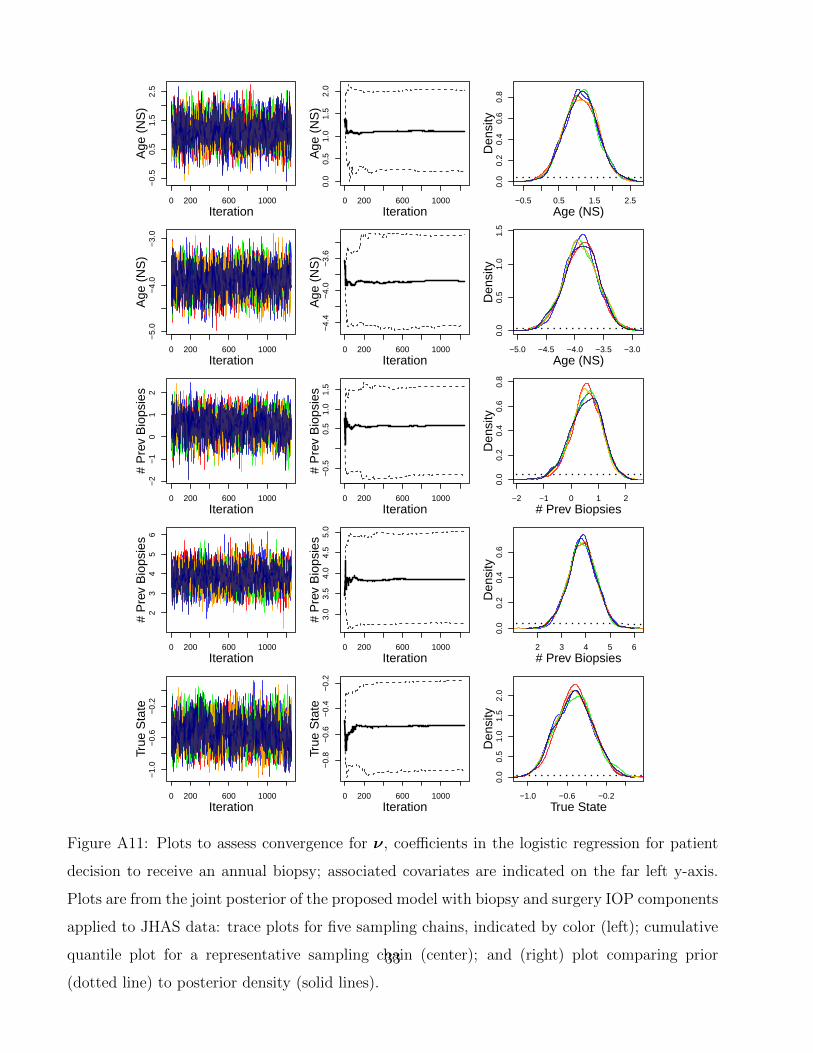
0 200 600 1000
−0.
50.
51.
52.
5
Iteration
Age
(N
S)
0 200 600 1000
0.0
0.5
1.0
1.5
2.0
Iteration
Age
(N
S)
−0.5 0.5 1.5 2.5
0.0
0.2
0.4
0.6
0.8
Den
sity
Age (NS)
0 200 600 1000
−5.
0−
4.0
−3.
0
Iteration
Age
(N
S)
0 200 600 1000
−4.
4−
4.0
−3.
6
Iteration
Age
(N
S)
−5.0 −4.5 −4.0 −3.5 −3.0
0.0
0.5
1.0
1.5
Den
sity
Age (NS)
0 200 600 1000
−2
−1
01
2
Iteration
# P
rev
Bio
psie
s
0 200 600 1000
−0.
50.
51.
01.
5
Iteration
# P
rev
Bio
psie
s
−2 −1 0 1 20.
00.
20.
40.
60.
8D
ensi
ty
# Prev Biopsies
0 200 600 1000
23
45
6
Iteration
# P
rev
Bio
psie
s
0 200 600 1000
3.0
3.5
4.0
4.5
5.0
Iteration
# P
rev
Bio
psie
s
2 3 4 5 6
0.0
0.2
0.4
0.6
Den
sity
# Prev Biopsies
0 200 600 1000
−1.
0−
0.6
−0.
2
Iteration
True
Sta
te
0 200 600 1000
−0.
8−
0.6
−0.
4−
0.2
Iteration
True
Sta
te
−1.0 −0.6 −0.2
0.0
0.5
1.0
1.5
2.0
Den
sity
True State
Figure A11: Plots to assess convergence for ν, coefficients in the logistic regression for patient
decision to receive an annual biopsy; associated covariates are indicated on the far left y-axis.
Plots are from the joint posterior of the proposed model with biopsy and surgery IOP components
applied to JHAS data: trace plots for five sampling chains, indicated by color (left); cumulative
quantile plot for a representative sampling chain (center); and (right) plot comparing prior
(dotted line) to posterior density (solid lines).
33
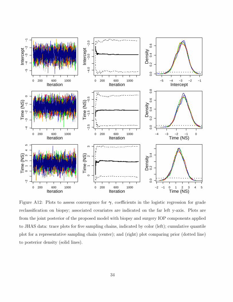
0 200 600 1000
−5
−4
−3
−2
−1
Iteration
Inte
rcep
t
0 200 600 1000
−4.
0−
3.0
−2.
0Iteration
Inte
rcep
t−5 −4 −3 −2 −1
0.0
0.2
0.4
0.6
Den
sity
Intercept
0 200 600 1000
−4
−3
−2
−1
0
Iteration
Tim
e (N
S)
0 200 600 1000
−2.
5−
1.5
−0.
5
Iteration
Tim
e (N
S)
−4 −3 −2 −1 0
0.0
0.2
0.4
0.6
0.8
Den
sity
Time (NS)
0 200 600 1000
−2
01
23
45
Iteration
Tim
e (N
S)
0 200 600 1000
01
23
Iteration
Tim
e (N
S)
−2 −1 0 1 2 3 4 5
0.0
0.2
0.4
Den
sity
Time (NS)
Figure A12: Plots to assess convergence for γ, coefficients in the logistic regression for grade
reclassification on biopsy; associated covariates are indicated on the far left y-axis. Plots are
from the joint posterior of the proposed model with biopsy and surgery IOP components applied
to JHAS data: trace plots for five sampling chains, indicated by color (left); cumulative quantile
plot for a representative sampling chain (center); and (right) plot comparing prior (dotted line)
to posterior density (solid lines).
34
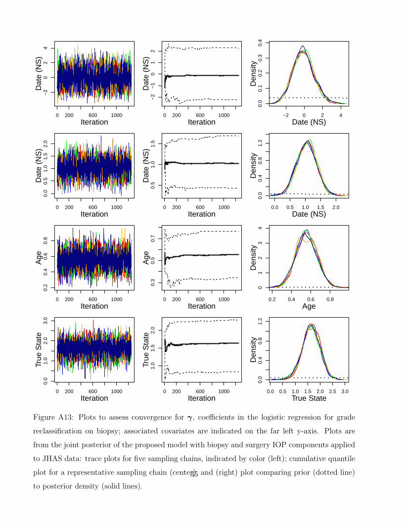
0 200 600 1000
−2
02
4
Iteration
Dat
e (N
S)
0 200 600 1000
−2
−1
01
2
Iteration
Dat
e (N
S)
−2 0 2 4
0.0
0.1
0.2
0.3
0.4
Den
sity
Date (NS)
0 200 600 1000
0.0
0.5
1.0
1.5
2.0
Iteration
Dat
e (N
S)
0 200 600 1000
0.5
1.0
1.5
Iteration
Dat
e (N
S)
0.0 0.5 1.0 1.5 2.0
0.0
0.4
0.8
1.2
Den
sity
Date (NS)
0 200 600 1000
0.2
0.4
0.6
0.8
Iteration
Age
0 200 600 1000
0.3
0.5
0.7
Iteration
Age
0.2 0.4 0.6 0.8
01
23
4D
ensi
ty
Age
0 200 600 1000
0.0
1.0
2.0
3.0
Iteration
True
Sta
te
0 200 600 1000
1.0
1.5
2.0
Iteration
True
Sta
te
0.0 0.5 1.0 1.5 2.0 2.5 3.0
0.0
0.4
0.8
1.2
Den
sity
True State
Figure A13: Plots to assess convergence for γ, coefficients in the logistic regression for grade
reclassification on biopsy; associated covariates are indicated on the far left y-axis. Plots are
from the joint posterior of the proposed model with biopsy and surgery IOP components applied
to JHAS data: trace plots for five sampling chains, indicated by color (left); cumulative quantile
plot for a representative sampling chain (center); and (right) plot comparing prior (dotted line)
to posterior density (solid lines).
35
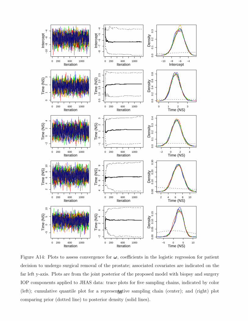
0 200 600 1000
−10
−8
−6
−4
Iteration
Inte
rcep
t
0 200 600 1000
−8
−7
−6
−5
−4
Iteration
Inte
rcep
t
−10 −8 −6 −4
0.0
0.1
0.2
0.3
Den
sity
Intercept
0 200 600 1000
01
23
Iteration
Tim
e (N
S)
0 200 600 1000
0.5
1.0
1.5
2.0
2.5
Iteration
Tim
e (N
S)
0 1 2 3
0.0
0.2
0.4
0.6
0.8
Den
sity
Time (NS)
0 200 600 1000
−2
02
4
Iteration
Tim
e (N
S)
0 200 600 1000
−1
01
23
Iteration
Tim
e (N
S)
−2 0 2 40.
00.
10.
20.
30.
4D
ensi
ty
Time (NS)
0 200 600 1000
24
68
10
Iteration
Tim
e (N
S)
0 200 600 1000
45
67
89
Iteration
Tim
e (N
S)
2 4 6 8 10
0.00
0.10
0.20
0.30
Den
sity
Time (NS)
0 200 600 1000
−5
05
10
Iteration
Tim
e (N
S)
0 200 600 1000
−2
02
46
Iteration
Tim
e (N
S)
−5 0 5 10
0.00
0.05
0.10
0.15
Den
sity
Time (NS)
Figure A14: Plots to assess convergence for ω, coefficients in the logistic regression for patient
decision to undergo surgical removal of the prostate; associated covariates are indicated on the
far left y-axis. Plots are from the joint posterior of the proposed model with biopsy and surgery
IOP components applied to JHAS data: trace plots for five sampling chains, indicated by color
(left); cumulative quantile plot for a representative sampling chain (center); and (right) plot
comparing prior (dotted line) to posterior density (solid lines).
36
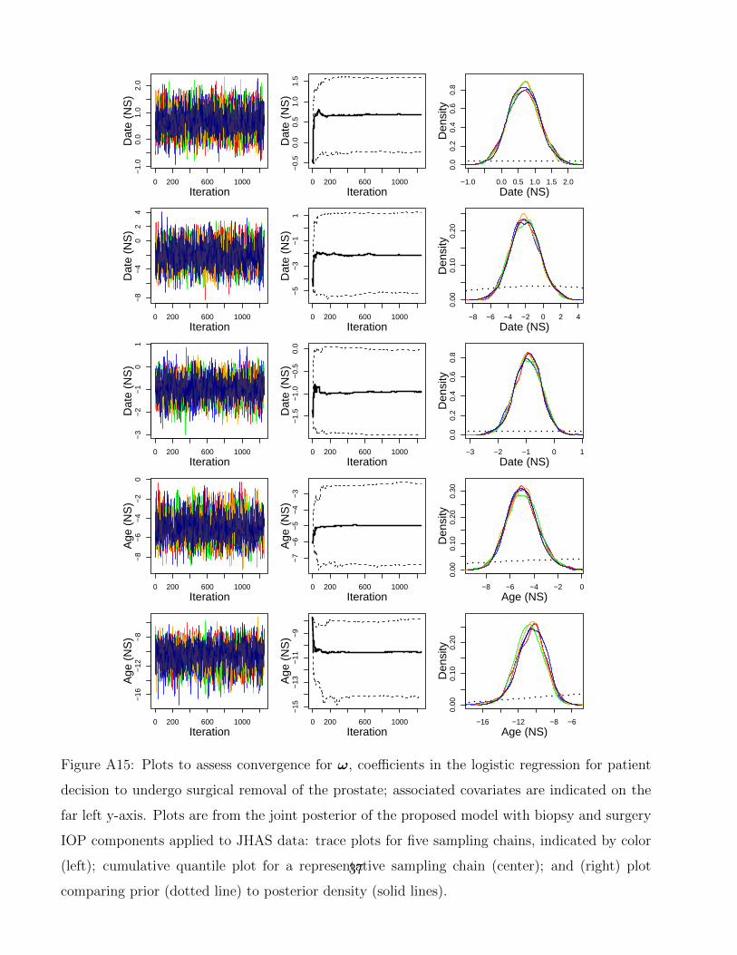
0 200 600 1000
−1.
00.
01.
02.
0
Iteration
Dat
e (N
S)
0 200 600 1000
−0.
50.
00.
51.
01.
5
Iteration
Dat
e (N
S)
−1.0 0.0 0.5 1.0 1.5 2.0
0.0
0.2
0.4
0.6
0.8
Den
sity
Date (NS)
0 200 600 1000
−8
−4
02
4
Iteration
Dat
e (N
S)
0 200 600 1000
−5
−3
−1
1
Iteration
Dat
e (N
S)
−8 −6 −4 −2 0 2 4
0.00
0.10
0.20
Den
sity
Date (NS)
0 200 600 1000
−3
−2
−1
01
Iteration
Dat
e (N
S)
0 200 600 1000
−1.
5−
1.0
−0.
50.
0
Iteration
Dat
e (N
S)
−3 −2 −1 0 10.
00.
20.
40.
60.
8D
ensi
ty
Date (NS)
0 200 600 1000
−8
−6
−4
−2
0
Iteration
Age
(N
S)
0 200 600 1000
−7
−6
−5
−4
−3
Iteration
Age
(N
S)
−8 −6 −4 −2 0
0.00
0.10
0.20
0.30
Den
sity
Age (NS)
0 200 600 1000
−16
−12
−8
Iteration
Age
(N
S)
0 200 600 1000
−15
−13
−11
−9
Iteration
Age
(N
S)
−16 −12 −8 −6
0.00
0.10
0.20
Den
sity
Age (NS)
Figure A15: Plots to assess convergence for ω, coefficients in the logistic regression for patient
decision to undergo surgical removal of the prostate; associated covariates are indicated on the
far left y-axis. Plots are from the joint posterior of the proposed model with biopsy and surgery
IOP components applied to JHAS data: trace plots for five sampling chains, indicated by color
(left); cumulative quantile plot for a representative sampling chain (center); and (right) plot
comparing prior (dotted line) to posterior density (solid lines).
37
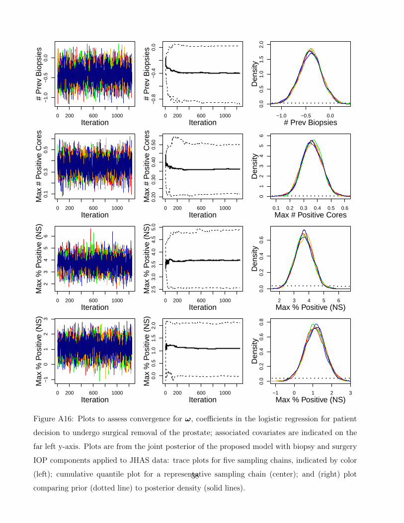
0 200 600 1000
−1.
0−
0.5
0.0
Iteration
# P
rev
Bio
psie
s
0 200 600 1000
−0.
8−
0.4
0.0
Iteration
# P
rev
Bio
psie
s
−1.0 −0.5 0.0
0.0
0.5
1.0
1.5
2.0
Den
sity
# Prev Biopsies
0 200 600 1000
0.1
0.3
0.5
Iteration
Max
# P
ositi
ve C
ores
0 200 600 1000
0.20
0.30
0.40
0.50
Iteration
Max
# P
ositi
ve C
ores
0.1 0.2 0.3 0.4 0.5 0.6
01
23
45
6D
ensi
ty
Max # Positive Cores
0 200 600 1000
23
45
6
Iteration
Max
% P
ositi
ve (
NS
)
0 200 600 1000
2.5
3.0
3.5
4.0
4.5
5.0
Iteration
Max
% P
ositi
ve (
NS
)
2 3 4 5 6
0.0
0.2
0.4
0.6
Den
sity
Max % Positive (NS)
0 200 600 1000
−1
01
23
Iteration
Max
% P
ositi
ve (
NS
)
0 200 600 1000
0.0
0.5
1.0
1.5
2.0
Iteration
Max
% P
ositi
ve (
NS
)
−1 0 1 2 3
0.0
0.2
0.4
0.6
0.8
Den
sity
Max % Positive (NS)
Figure A16: Plots to assess convergence for ω, coefficients in the logistic regression for patient
decision to undergo surgical removal of the prostate; associated covariates are indicated on the
far left y-axis. Plots are from the joint posterior of the proposed model with biopsy and surgery
IOP components applied to JHAS data: trace plots for five sampling chains, indicated by color
(left); cumulative quantile plot for a representative sampling chain (center); and (right) plot
comparing prior (dotted line) to posterior density (solid lines).
38
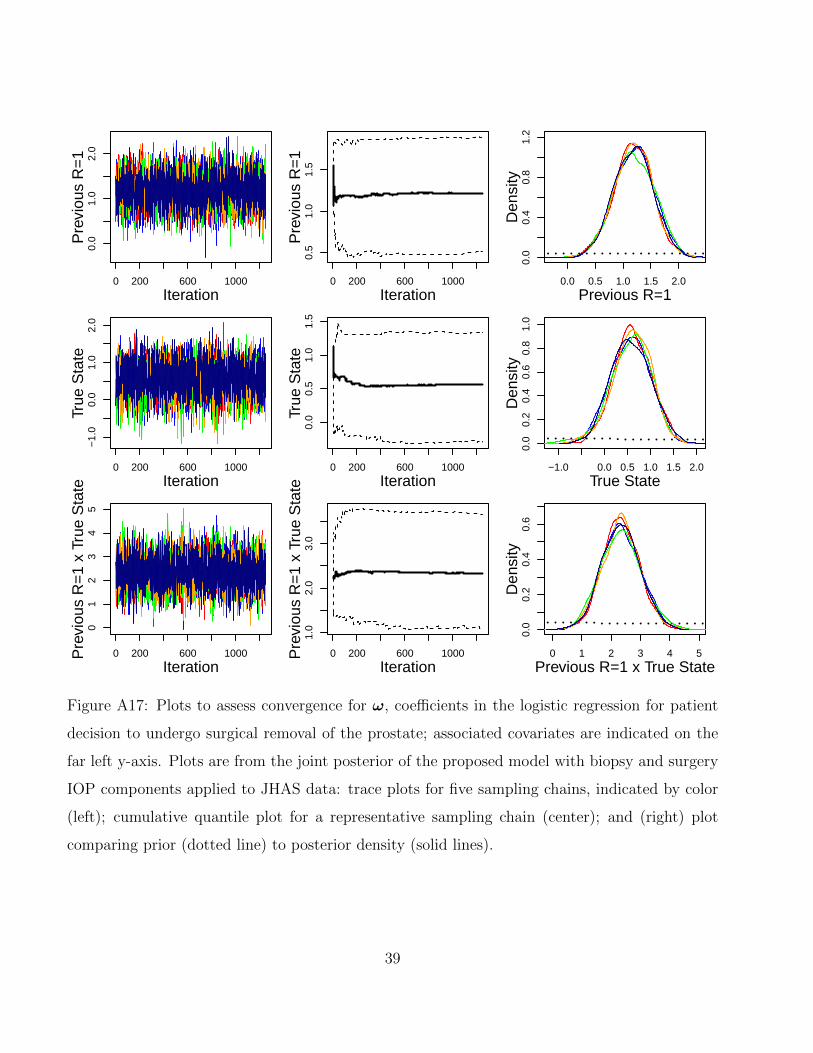
0 200 600 1000
0.0
1.0
2.0
Iteration
Pre
viou
s R
=1
0 200 600 1000
0.5
1.0
1.5
IterationP
revi
ous
R=
10.0 0.5 1.0 1.5 2.0
0.0
0.4
0.8
1.2
Den
sity
Previous R=1
0 200 600 1000
−1.
00.
01.
02.
0
Iteration
True
Sta
te
0 200 600 1000
0.0
0.5
1.0
1.5
Iteration
True
Sta
te
−1.0 0.0 0.5 1.0 1.5 2.0
0.0
0.2
0.4
0.6
0.8
1.0
Den
sity
True State
0 200 600 1000
01
23
45
Iteration
Pre
viou
s R
=1
x Tr
ue S
tate
0 200 600 1000
1.0
2.0
3.0
Iteration
Pre
viou
s R
=1
x Tr
ue S
tate
0 1 2 3 4 5
0.0
0.2
0.4
0.6
Den
sity
Previous R=1 x True State
Figure A17: Plots to assess convergence for ω, coefficients in the logistic regression for patient
decision to undergo surgical removal of the prostate; associated covariates are indicated on the
far left y-axis. Plots are from the joint posterior of the proposed model with biopsy and surgery
IOP components applied to JHAS data: trace plots for five sampling chains, indicated by color
(left); cumulative quantile plot for a representative sampling chain (center); and (right) plot
comparing prior (dotted line) to posterior density (solid lines).
39
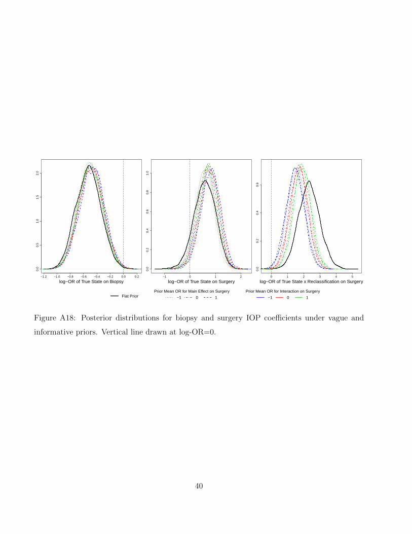
−1.2 −1.0 −0.8 −0.6 −0.4 −0.2 0.0 0.2
0.0
0.5
1.0
1.5
2.0
log−OR of True State on Biopsy−1 0 1 2
0.0
0.2
0.4
0.6
0.8
1.0
log−OR of True State on Surgery0 1 2 3 4 5
0.0
0.2
0.4
0.6
log−OR of True State x Reclassification on Surgery
Flat PriorPrior Mean OR for Main Effect on Surgery
−1 0 1
Prior Mean OR for Interaction on Surgery
−1 0 1
Figure A18: Posterior distributions for biopsy and surgery IOP coefficients under vague and
informative priors. Vertical line drawn at log-OR=0.
40
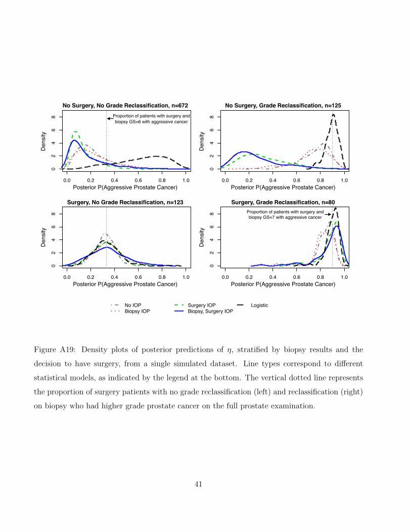
0.0 0.2 0.4 0.6 0.8 1.0
02
46
8
0.0 0.2 0.4 0.6 0.8 1.0
02
46
8
0.0 0.2 0.4 0.6 0.8 1.0
02
46
8
0.0 0.2 0.4 0.6 0.8 1.0
02
46
8
No IOPBiopsy IOP
Surgery IOPBiopsy, Surgery IOP
Logistic
Posterior P(Aggressive Prostate Cancer)
Posterior P(Aggressive Prostate Cancer) Posterior P(Aggressive Prostate Cancer)
Posterior P(Aggressive Prostate Cancer)
Den
sity
Den
sity
Den
sity
Den
sity
No Surgery, No Grade Reclassification, n=672
Surgery, No Grade Reclassification, n=123
No Surgery, Grade Reclassification, n=125
Surgery, Grade Reclassification, n=80
Proportion of patients with surgery and biopsy GS=6 with aggressive cancer
Proportion of patients with surgery and biopsy GS=7 with aggressive cancer
Figure A19: Density plots of posterior predictions of η, stratified by biopsy results and the
decision to have surgery, from a single simulated dataset. Line types correspond to different
statistical models, as indicated by the legend at the bottom. The vertical dotted line represents
the proportion of surgery patients with no grade reclassification (left) and reclassification (right)
on biopsy who had higher grade prostate cancer on the full prostate examination.
41
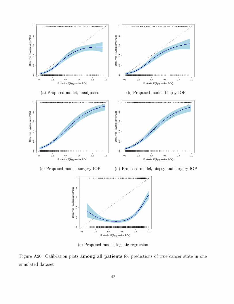
Posterior P(Aggressive PCa)
Obs
erve
d P
(Agg
ress
ive
PC
a)
0.0 0.2 0.4 0.6 0.8 1.0
0.0
0.2
0.4
0.6
0.8
1.0
(a) Proposed model, unadjusted
Posterior P(Aggressive PCa)
Obs
erve
d P
(Agg
ress
ive
PC
a)
0.0 0.2 0.4 0.6 0.8 1.0
0.0
0.2
0.4
0.6
0.8
1.0
(b) Proposed model, biopsy IOP
Posterior P(Aggressive PCa)
Obs
erve
d P
(Agg
ress
ive
PC
a)
0.0 0.2 0.4 0.6 0.8 1.0
0.0
0.2
0.4
0.6
0.8
1.0
(c) Proposed model, surgery IOP
Posterior P(Aggressive PCa)
Obs
erve
d P
(Agg
ress
ive
PC
a)
0.0 0.2 0.4 0.6 0.8 1.0
0.0
0.2
0.4
0.6
0.8
1.0
(d) Proposed model, biopsy and surgery IOP
Posterior P(Aggressive PCa)
Obs
erve
d P
(Agg
ress
ive
PC
a)
0.0 0.2 0.4 0.6 0.8 1.0
0.0
0.2
0.4
0.6
0.8
1.0
(e) Proposed model, logistic regression
Figure A20: Calibration plots among all patients for predictions of true cancer state in one
simulated dataset
42
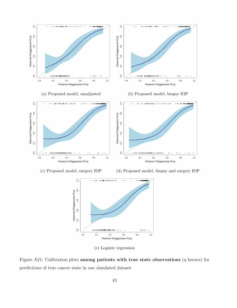
Posterior P(Aggressive PCa)
Obs
erve
d P
(Agg
ress
ive
PC
a)
0.0 0.2 0.4 0.6 0.8 1.0
0.0
0.2
0.4
0.6
0.8
1.0
(a) Proposed model, unadjusted
Posterior P(Aggressive PCa)
Obs
erve
d P
(Agg
ress
ive
PC
a)
0.0 0.2 0.4 0.6 0.8 1.0
0.0
0.2
0.4
0.6
0.8
1.0
(b) Proposed model, biopsy IOP
Posterior P(Aggressive PCa)
Obs
erve
d P
(Agg
ress
ive
PC
a)
0.0 0.2 0.4 0.6 0.8 1.0
0.0
0.2
0.4
0.6
0.8
1.0
(c) Proposed model, surgery IOP
Posterior P(Aggressive PCa)
Obs
erve
d P
(Agg
ress
ive
PC
a)
0.0 0.2 0.4 0.6 0.8 1.0
0.0
0.2
0.4
0.6
0.8
1.0
(d) Proposed model, biopsy and surgery IOP
Posterior P(Aggressive PCa)
Obs
erve
d P
(Agg
ress
ive
PC
a)
0.0 0.2 0.4 0.6 0.8 1.0
0.0
0.2
0.4
0.6
0.8
1.0
(e) Logistic regression
Figure A21: Calibration plots among patients with true state observations (η known) for
predictions of true cancer state in one simulated dataset
43
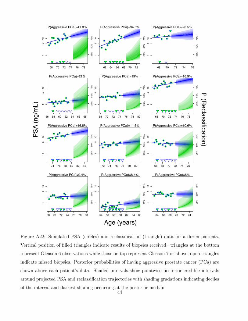
Age (years)
PSA
(ng/
mL)
P (Reclassification)
●●
●●
●●
●●
●
●●
●●
68 70 72 74 76 78
15
10
P(Aggressive PCa)=41.8%
●●
●●
●●
●●
●
●●
●●
25%
50%
75%
●
●
●
●●● ●
●●
●●
●●
62 64 66 68 70 72
15
10
P(Aggressive PCa)=34.5%
●
●
●
●●● ●
●●
●●
●●
25%
50%
75% ● ●
●
●
●
●
●
68 70 72 74 76
15
10
P(Aggressive PCa)=28.5%
● ●●
●
●
●
●
25%
50%
75%
●
●●
●
●●●●● ●
●
●●
56 58 60 62 64 66 68
15
10
P(Aggressive PCa)=21%
●
●●
●
●●●●● ●
●
●●
25%
50%
75%
●● ●
●
● ●●●●●
●
●
68 70 72 74 76 78 80
15
10
P(Aggressive PCa)=19%
●● ●
●
● ●●●●●
●
●
25%
50%
75%
●
●
●●
●●
●●
●●
●●
68 70 72 74 76 78
15
10
P(Aggressive PCa)=16.9%
●
●
●●
●●
●●
●●
●●
25%
50%
75%
●●
●
●
●
●●
●●●●●
74 76 78 80 82 84
15
10
P(Aggressive PCa)=16.8%
●●
●
●
●
●●
●●●●●
25%
50%
75%
●
●
●●
●●●
●●●●
●●
72 74 76 78 80 82
15
10
P(Aggressive PCa)=11.6%
●
●
●●
●●●
●●●●
●●25
%50
%75
%●
●●
●●●
●
●
●●●●
66 68 70 72 74 76
15
10
P(Aggressive PCa)=10.6%
●
●●
●●●
●
●
●●●●
25%
50%
75%
●
●●●
● ●●●●
●●
●
68 70 72 74 76 78 80
15
10
P(Aggressive PCa)=9.4%
●
●●●
● ●●●●
●●
●
25%
50%
75%
●● ●
●
●
● ●●●●●
●
54 56 58 60 62 64 66
15
10
P(Aggressive PCa)=8.4%
●● ●
●
●
● ●●●●●
● 25%
50%
75%
●●
●●●●●
●●● ●
●●
64 66 68 70 72 74
15
10
P(Aggressive PCa)=6%
●●
●●●●●
●●● ●
●●
25%
50%
75%
Figure A22: Simulated PSA (circles) and reclassification (triangle) data for a dozen patients.
Vertical position of filled triangles indicate results of biopsies received– triangles at the bottom
represent Gleason 6 observations while those on top represent Gleason 7 or above; open triangles
indicate missed biopsies. Posterior probabilities of having aggressive prostate cancer (PCa) are
shown above each patient’s data. Shaded intervals show pointwise posterior credible intervals
around projected PSA and reclassification trajectories with shading gradations indicating deciles
of the interval and darkest shading occurring at the posterior median.44