ACT Working Paper Series

ACT working papers document preliminary research. The papers are intended to promote discussion and feedback before formal publication. The research does not necessarily reflect the views of ACT.

A Bayesian Hierarchical Selection Model for Academic Growth with Missing Data Jeff Allen WP-2015-04 April, 2015

A Bayesian Hierarchical Selection Model for Academic Growth with Missing Data

Jeff Allen April 2015

Abstract

Using a sample of schools testing annually in grades 9-11 with a vertically-linked series

of assessments, a latent growth curve model is used to model test scores with student intercepts

and slopes nested within school. Missed assessments can occur because of student mobility,

student dropout, absenteeism, and other reasons. Missing data indicators are modeled using

logistic regression, with grade 9 and potentially unobserved growth scores used as covariates.

Under a hierarchical selection model, estimates of school effects on academic growth and

missingness are obtained. The results from the selection model are compared to a model that

ignores the missing data process.

The author would like to acknowledge Ruitao Liu and Justine Radunzel for their review and

helpful comments on this report.

KEY WORDS: selection model, latent growth curve, hierarchical model, not missing at random,

informative missingness, school effectiveness, Bayesian analysis, WinBUGS

2

Introduction

Educators, researchers, and policymakers are increasingly interested in measures of

academic growth for purposes of monitoring student progress, evaluating interventions, and

measuring school or teacher effectiveness. Growth models require longitudinal data systems that

track assessment data over time and link the data to individual students, teachers, and schools.

Not unlike longitudinal data in other disciplines, missing data are common with academic

assessment because of student migration out of the school system, sickness, truancy, and student

dropout, among other reasons.

Customary methods for analyzing longitudinal data assume that data are missing at

random – that is, missingness depends only on the observed responses and covariates. However,

in the case of longitudinal assessment data, it is plausible that missingness is related to

unobserved level of academic achievement. Academic difficulty or lack of academic growth

could contribute to students leaving high school or missing assessment days. Alternatively, other

student risk factors could affect both academic performance and likelihood of missing

assessment days. If academic performance is the outcome of interest amd unobserved academic

performance constructs are related to missingness, data are not missing at random.

In this paper, a Bayesian approach is presented for jointly modeling the academic growth

and missing data processes in an attempt to account for informative missingness. Using

WinBUGS, the model was fit for a sample of schools that test annually in grades 9-11 with a

series of vertically-scaled assessments. The results are compared to those from a simpler model

that ignores the missing data process, with emphasis on measures of school effects on academic

growth.

3

Informative dropout in longitudinal research

This study deals with a common situation where the primary outcome is measured on

individuals at multiple time points, and that the research focuses on examining predictors of

change in the outcome. Random coefficient models are often used for this purpose. For

example, each individual’s vector of outcomes can be described by a person-specific intercept,

slope, and possible higher-order terms. The individual effects are not observed and this type of

model is also known as a latent growth curve model.

A common problem that arises in longitudinal studies is missing data in the primary

outcome. Using maximum likelihood estimation on the observed data set results in unbiased

estimation when the missingness process only depends on observed data and other observed

covariates. This situation is known as missing at random (Little, 1995). Unfortunately, it is

often plausible that the missing data process depends on the unobserved data. In this case, the

data are not missing at random (Little, 1995), and estimation of the rate of change parameters

may be biased. For example, in medical research, not missing at random can result when

dropout is caused by illness or death. In an educational research example, not missing at random

can result when missed assessments are influenced by students’ expected academic performance.

Wu & Bailey (1988) defined informative right censoring to refer to situations where the

probability of dropping out depends on an individual's slope. Note that dropout is a specific type

of missing data situation, where Y is no longer observed after time of dropout; in other cases

intermittent missingness is possible.

Methods have been developed that attempt to correct the bias caused by not missing at

random, which is also referred to as non-ignorable missingness or informative missingness. Two

general types of models have been proposed: selection models, in which the missingness process

4

is modeled simultaneously with the outcome data process; and pattern-mixture models (c.f.,

Hedeker & Gibbons, 1997), which estimate the parameters of interest separately for each missing

data pattern and then calculate overall estimates by averaging over the missing data patterns.

This paper focuses on a type of selection model.

Selection models work by explicitly modeling the missing data process, with missing

outcome data or latent variables used as predictors of missingness. When missing data depends

on missing response variables, the situation is called outcome-dependent missingness; random-

coefficient-dependent missingness occurs when the missing data depends on random effects or

latent variables (Feldman & Rabe-Hesketh, 2012). When the missing data process depends on

random effects or latent variables, the model is also called a shared parameter model because the

random effects are used to describe the primary outcome measure and also used as predictors of

missingness.

Studies of the performance of selection models generally find that models that ignore the

missing data process result in bias associated with the rate of change (slope) parameters and that

this bias increases as the relation between person-specific slopes and dropout becomes stronger,

and when the proportion of subjects with fewer than two observations increases (Saha & Jones,

2005). In simulation studies, the true dropout process is known, and so the performance of

different selection models can be studied under different scenarios. The studies have shown that

the bias is diminished or eliminated by using selection models to jointly model the longitudinal

outcome of interest and dropout data. In reality, the true dropout process is not known, so theory

and judgment must be used to specify the model. Because of this subjectivity, it is recommended

that researchers perform sensitivity analyses to examine the study results under a variety of

assumed models (Molenberghs & Kenward, 2007; Xu & Blozis, 2011).

5

There are many variants of selection models, characterized by the model used for the

primary outcome, the model used for the missing data process, the selection of predictors of

missing data, and the hierarchical structure of the outcome and missingness models. Selection

models first gained popularity in medical research. Wu & Carroll (1988) introduced the shared

parameter model for analyzing rates of change of a continuous outcome between two groups.

They used random subject effects (person-specific intercept and slope parameters) to model the

continuous outcome and used the same random effects as predictors of study dropout. Mori,

Woolson, & Woodworth (1994) used the shared parameter approach with a random slope model

where each subject's number of measurements was modeled using the truncated geometric

distribution. Diggle & Kenward (1994) specified an outcome-dependent missingness model with

a multivariate linear model for the outcome and a logistic regression model for the dropout

process. Predictors of dropout included the outcome at the time of dropout as well as the

outcome measured at the time prior to dropout. Pulkstenis, Ten Have, & Landis (1998) fit a

mixed effects logistic model to binary longitudinal data sharing parameters with a discrete-time

survival model for the dropout process. Albert & Follmann (2000) used the shared parameter

approach for repeated Poisson outcomes with informative dropout. Wang & Taylor (2001)

proposed a joint model for longitudinal and event time data that allows the person-specific slopes

to vary over time. They specified prior distributions and fit their model using MCMC methods.

More recently, selection models have gained momentum in educational research. Tanaka

and Kanazawa (2010) analyzed grade 7 to grade 10 test score data using a latent growth curve

model with dropout modeled using a logistic regression survival process depending on student

intercepts and slopes. The model was specified and fit using Bayesian methods. McCaffrey and

Lockwood (2011) studied grade 1-5 math score data with a focus on estimating teacher effects.

6

They specified two selection models: one modeling the number of observed test scores

dependent on an unobserved student effect, and the other modeling each instance of test score

missingness as binary random variable with logistic link function, again dependent on the

unobserved student effect. They also studied a pattern-mixture model and discussed the

sensitivity of their results to model specification. They found that the selection models and

pattern-mixture models did not have much effect on estimated teacher effects. Xu and Blozis

(2011) analyzed procedural learning task performance over time. They contrasted results from

complete-case analysis (discarding observations with missing data), models that used the

complete data set but assumed missing at random, selection models assuming outcome-

dependent missingness, and a pattern-mixture model. Results changed appreciably when using

the complete-case analysis, but were more stable across the selection models and model that

assumed missing at random. Feldman and Rabe-Hesketh (2012) analyzed reading test score data

from the NELS:88 longitudinal study using a latent growth curve model for the growth process

and a logistic model for the dropout process with student intercepts and slopes included as

predictors of dropout. They found that both intercepts and slopes were inversely related to risk

of dropout, but that the parameter estimates of the growth model were quite similar for the

regular model (that assumes missing at random and ignores the dropout process) and the shared

parameter model. Karl, Yang, and Lohr (2013) fit a correlated parameter model, where the

model for the primary outcome (test scores) depended on latent student and teacher effects, the

model for missingness depended on different latent student and teacher effects, and the two sets

of latent effects are allowed to be correlated. The correlated parameter model is considered a

generalization of the shared parameter model.

7

Research questions

The primary goal of this study is to determine the extent that accounting for informative

missingness affects measures of student and school growth for a particular assessment system.

The primary research questions addressed are:

1) To what extent does accounting for informative missingness affect school effectiveness

estimates?

2) To what extent does accounting for informative missingness affect individual student growth

estimates?

Method

Sample and data

School systems that use ACT’s College and Career Readiness System and test students

each year with ACT Explore (grade 9), ACT Plan (grade 10), and the ACT College Readiness

Assessment (grade 11) are the focus of this study. The three assessments share a common score

scale, with different score ceilings. Explore scores range from 1-25, Plan scores range from 1-

32, and ACT scores range from 1-36. Explore, Plan, and the ACT all contain multiple choice

tests in English, Mathematics, Reading, and Science. The philosophical basis for the tests are

that (a) the tests should measure academic skills necessary for education and work after high

school and (b) the content of the tests should be related to major curriculum areas (ACT, 2013).

For each assessment, the Composite score is calculated as the mean of the four subject area

scores. The ACT focuses on the knowledge and skills attained as the cumulative effect of school

experience. Plan is intended for all 10th graders and focuses on the knowledge and skills that are

typically attained by grade 10, and Explore is intended for all students in grades 8 and 9 and

focuses on the knowledge and skills that are usually attained by grade 8.

8

High schools with all-student testing programs in grades 9-11 are the focus of this study.

Specifically, high schools that tested their 2012 high school graduating class with Explore in

2008-2009 (grade 9), Plan in 2009-2010 (grade 10), and the ACT in spring 2011 (grade 11) were

included. Some students also elected to take the ACT in grade 12 and those test scores are

included in the analysis. To determine if a high school had an all-student testing program, the

proportion tested for grades 9, 10, and 11 was calculated. Proportion tested was defined as the

number of tested students, divided by grade level enrollment.1 Schools whose proportion tested

was at least 0.75 for all three grade levels and located in a state that administers the ACT to all

grade 11 students were included. The resulting sample of 223 high schools is summarized in

Table 1 with respect to school percent eligible for free or reduced lunch, student sample size, and

test score missingness for grades 9-12. There was considerable variation in the within-school

sample sizes, with 13.9% of the schools having fewer than 40 students and 16.1% having more

than 300. Most schools were in the 40-79 (25.6%) or 80-159 (29.1%) sample size ranges.

Schools also varied with respect to poverty level (measured by percent eligible for free or

reduced lunch), with 25.6% at 0-19%, 52.5% at 20-39%, 21.1% at 40-69%, and just 0.9% at 70%

or higher. The mean percentage of students tested was 84.5% (SD=8.3) for grade 10 and 79.4%

(SD=6.7) for grade 11. The mean percentage of students tested in grade 12 was 13.0% as

relatively few students elected to test again in grade 12.

Students were included in the study if they took ACT Explore in grade 9 and were

allocated to the high school they attended at that time. Because measures of school effectiveness

are of interest in this study, only students whose academic growth could be attributed to a single

high school were included. Thus, if a student was affiliated with more than one high school

1 Grade level enrollment data was obtained from the National Center for Education Statistics Common Core of Data School Database.

9

during grades 9-12, they were removed from the data set. The resulting sample of 35,286

students is summarized in Table 1 with respect to gender, ethnicity, mean test scores, and

proportion missing test scores at grades 9-12. The sample was evenly distributed by gender,

with 75.4% Caucasian, 11.9% Hispanic, 6.8% other race/ethnicity, 4.0% African American, and

1.9% unknown race/ethnicity. Compared to the national population of high school students, the

sample has relatively more Caucasian and relatively fewer African American students. The

mean Composite scores are 16.6 for grade 9, 18.4 for grade 10, 20.9 for grade 11, and 22.5 for

grade 12. Because the number of students tested decreases with grade level, the simple means do

not accurately portray average growth patterns. If lower achieving students are more likely to

miss assessments, the simple means would suggest a higher level of growth than what would be

observed if all students tested at each grade level.

10

Table 1: Sample Description

High Schools Number of Students No. % Mean SD 10-39 31 13.9 40-79 57 25.6 80-159 65 29.1 160-299 34 15.2 300+ 36 16.1 Poverty level No. % Mean SD 0-19% 57 25.6 20-39% 117 52.5 40-69% 47 21.1 70%+ 2 0.9 Percent tested Mean SD Grade 9 100.0 0.0 Grade 10 84.5 8.3 Grade 11 79.4 6.7 Grade 12 13.0 7.6

Students Gender No. % Mean SD Female 17,250 48.9 Male 17,962 50.9 Unknown 74 0.2 Race/ethnicity No. % Mean SD African American 1,423 4.0 Caucasian 26,591 75.4 Hispanic 4,195 11.9 Other 2,391 6.8 Unknown 686 1.9 Test scores No. % Mean SD Grade 9 35,286 100.0 16.6 3.4 Grade 10 30,048 85.2 18.4 3.8 Grade 11 27,977 79.3 20.9 5.1 Grade 12 5,565 15.8 22.5 4.6

Because of the study inclusion criteria, all students had a baseline measurement (grade 9

test score). There were eight possible missing data patterns and the relative frequency of each is

summarized in Table 2. A majority of students (61.6%) tested in grades 9-11, but not in grade

12 (note that the grade 12 test is not part of the all-student testing program). Another set of

11

students, 14.7%, tested in all four grade levels. Not including the grade 12 missingness, the most

common missing data pattern (11.8%) was to test in grade 9, but then to miss grades 10-12. The

next most common pattern (8.3%) was to test in grades 9 and 10, but then to miss the grade 11

and 12 tests. The most common intermittent missing data pattern (2.6%) was to miss the grade

10 and grade 12 tests, but to test in grade 11. Data indicating reasons for missed assessments

was not available, but plausible reasons for missing data include high school dropout, migration

out of the high school, absenteeism on test day, opting out of testing, and being held back.

Table 2: Missing Data Patterns (O=test score missing, X=test score observed)

Selection model for assessment data with missingness

Selection models for informative missingness have two components: the longitudinal

outcome component (test scores in our case) and the dropout/missingness component (indicators

for missed assessments in our case). These two components are described separately and prior

distributions for the model parameters are then specified. The model was fit using the Bayesian

framework, which provides two key advantages: 1) reliable statistical inference with no reliance

on asymptotic theory, and 2) a flexible framework for conducting sensitivity analysis of model

specification and prior distributions.

Missing Data Pattern N %

9 10 11 12 X O O O 4,149 11.8 X X O O 2,917 8.3 X O X O 917 2.6 X O O X 45 0.0 X X X O 21,738 61.6 X X O X 198 0.6 X O X X 127 0.4 X X X X 5,195 14.7

Total 35,286 100.0

12

Hierarchical linear model for test score data. The assessment data include subject-

specific scores for English, Mathematics, Reading, and Science as well as a Composite score.

Because school effects on overall academic readiness are of interest and to simplify the analysis,

only Composite scores are used. The Composite score for the ith student from the jth school in

the kth year of high school (k=1,2,3,4) is denoted yijk. With the common score scale used by the

Explore, Plan, and ACT assessments, a random coefficients model (Raudenbush & Bryk, 2002)

is assumed so that initial academic performance (grade 9 score) and rate of change (slope) vary

across students and high schools. Specifically,

Equation 1: Level 1 Model for Test Scores 𝑦𝑖𝑖𝑖~𝑁�𝑏0𝑖𝑖 + 𝑡𝑖𝑖𝑖𝑏1𝑖𝑖 ,σ2�

where 𝑏0𝑖𝑖 is the initial level of academic performance (intercept parameter) and 𝑏1𝑖𝑖 is the rate

of change in academic performance (slope parameter) for the ith student from the jth school. The

number of months elapsed (not counting the three months of summer) since the start of high

school (assumed to be September 1st of grade 9) is denoted 𝑡𝑖𝑖𝑖. This model is also referred to as

a random intercepts and slopes model, a linear latent growth curve model, or a normal

hierarchical linear model. The model assumes that deviations from each student’s linear

trajectory are normally distributed with variance σ2. Each student's intercept and slope is

assumed to be a drawn from a bivariate normal distribution, with school-specific means and

unstructured covariance matrix bΣ :

Equation 2: Level 2 Model for Student Intercepts and Slopes

ΣΣ

ΣΣ

=Σ

22

12

12

11

1

0

1

0 ,~ bj

j

ij

ij

rr

Nbb

where 𝑟0𝑖 is the mean initial level of academic performance (school mean intercept) and 𝑟1𝑖 is

the mean rate of change in academic performance (school mean slope) for the jth school. The

13

school intercepts and slopes are assumed to be drawn from a bivariate normal distribution, with

means modeled as a function of school poverty level (proportion of students eligible for free or

reduced lunch) and unstructured covariance matrix rΣ :

Equation 3: Level 3 Model for School Intercepts and Slopes

=Σ

×+

×+

22

12

12

11

43

10

1

0 ,~ηη

ηη

ββ

ββr

j

j

j

j

FRLFRL

Nrr

With this model specification, estimates of ijb1 represent student growth measures, and estimates

of jr1 are school growth measures. Under the assumption that student growth is attributed to

schools, the school growth measure could be used as a measure of school effectiveness. A

school effectiveness measure adjusted for school poverty level is then calculated as

( )jj FRLr ×+− 431 ββ .

Logistic regression models for missing data. Our data set includes indicators of

whether students tested at grades 10, 11, and 12 (everyone tested at grade 9). Let ijkm be the test

score non-missing indicator ( 0=ijkm if missing, 1=ijkm if not missing) for the ith student from

the jth school at year k (k=2,3,4 for grades 10, 11, and 12 respectively). Because missing the

assessments is plausibly related to performance on the assessments, the missing data indicators

are modeled as Bernoulli random variables with the probability of missing the assessment

dependent on the baseline test score (grade 9 Composite score) and change from baseline (grade

8+k Composite score - grade 9 Composite score). Because schools might have effects on

missingness that are unrelated to test scores, school-specific intercepts are allowed. Logistic

regression was used with the following specification of the logit function:

Equation 4: Logit Function for Missing Data Models

( )12110 ijijkkijkkjijk yyymL −++= αα

14

This model specifies that the probability of missing an assessment depends on the test score at

time k, which is potentially unobserved. Because the effects of academic performance on

missing assessments are potentially different at grades 10, 11, and 12, the model also allows the

missingness parameters to vary by time. The school effects on missing data are assumed to be

drawn from a bivariate normal distribution with covariance matrix mΣ :

Equation 5: Level 2 Model for School Effects on Missingness

=Σ

3323

2322

1312

13

12

11

04

03

02

04

03

02

,~λλλλλλ

λλλ

ααα

m

j

j

j

Nmmm

Because the test scores are the focus of the hierarchical response model and are included as

predictors in the missing data model, the full model specification is characterized as a selection

model with outcome-dependent missingness, such as in Diggle & Kenward (1994) and Xu and

Blozis (2011).

Prior distributions. Our general strategy for specifying prior distributions was to only

use informative priors when such priors are needed to obtain proper posterior distributions.

Hobert & Casella (1996) have shown that, for normal hierarchical linear models such as ours,

proper prior distributions on these covariance matrices are needed for a proper joint posterior

distribution. Therefore, informative priors were specified for the covariance matrices of student

intercepts and slopes ( bΣ ), school mean intercepts and slopes ( rΣ ), and school effects on

missingness ( mΣ ). Note that WinBUGS requires us to specify variance components using

precisions (inverses of variances). Using a parametrization given by Carlin & Louis (pp. 166-

168, 1996), a Wishart prior distribution is specified for the inverses of the covariance matrices as

Equation 6: Wishart Priors for Covariance Matrices

( ){ }κκ ,~ 11 −−Σ RW

15

where κ is a degree of freedom parameter that represents the effective sample size. By setting

20=κ , our prior distributions have about the same influence as an observed data likelihood for

n=20. Using the parametrization given in Equation 6, the prior mean of 1−Σ is 1−R . To obtain

the prior means for bΣ and rΣ parameter values are elicited from subject matter experts. Two

senior ACT researchers with 10+ years of experience working with Explore, Plan, and ACT data

were asked to complete the prior elicitation exercise presented in Appendix A, yielding a priori

estimates of the variance components. One expert completed the exercise based on personal

experience and without performing any analysis or consulting related research findings, while

the other completed the exercise by performing some analyses using data independent of the data

used in this study. The model was fit using the prior distributions elicited from the first expert

and then sensitivity to the prior was checked by comparing the results against those obtained by

using the prior distributions elicited from the second expert. The prior mean for the variance

components of the school effects on missingness were obtained by analyzing a dataset of high

school enrollment counts for a single cohort of students from grades 9 through 122.

For the other model parameters, proper prior distributions were not needed to obtain

proper posterior distributions. For 𝛽 and 𝛼, multivariate normal priors were specified with mean

0 and covariance matrix I910 . Note that the large prior variances ensure that the prior

distributions will have virtually no influence on the posterior distributions. For ( ) 12 −σ , a gamma

prior was specified with parameters 1 and 10-9, such that the prior density function is

approximately proportional to 1, and hence has virtually no influence on the posteriors.

2 High school enrollment count data from the National Center for Educational Statistics Common Core of Data were analyzed. Grade 10, 11, and 12 enrollment counts were modeled as binomial random variables with number of trials given by grade 9 enrollment count. School poverty level was controlled and school effects were estimated for each grade level, and then the covariance matrix of school effects on enrollment was estimated.

16

Model fitting with WinBUGs

Using Markov Chain Monte Carlo (MCMC) methods, parameter estimates were obtained

by simulating from the joint posterior distribution of the model parameters using the WinBUGS

software (Spiegelhalter, Thomas, Best, & Lunn, 2003). In addition to the selection model, a

simpler model was fit that ignores the missing data and thus assumes that the data are missing at

random. The simple model was also fit using WinBUGS and, with the exception of the missing

data component, the model specification and syntax is identical to that of the selection model.

MCMC methods require starting values for the model parameters. To obtain starting values for

the growth model parameters, the simple model was fit using SAS PROC MIXED. To obtain

starting values for the missing data component, random-effects logistic regression models were

fit using SAS GLIMMIX after imputing missing test scores.

A single chain was used so that only one set of starting values was needed. For the

selection model and simple model, 10,000 burn-in iterations were run to achieve sampling from

the stationary posterior distribution. To test for lack of convergence, Geweke's (1992) diagnostic

test was used on each of the model’s parameters. This test did not suggest lack of convergence

for any of the model’s parameters. Then, 10,000 iterations were run to obtain a large sample of

posterior draws. With 10,000 posterior draws, the sampling error in estimating the posterior

mean was less than one tenth of the estimated posterior standard deviation for all parameters.

Results

Using the MCMC approach, the posterior distribution of each unobserved parameter and

unobserved outcome is simulated. The posterior mean is used as the estimate, and the posterior

standard deviation serves as the standard error of the estimate. In Table 4, the growth model

parameter estimates are presented for the selection model and the simple model that assumes

17

missing at random. The slope parameter estimates are modestly different for the two models,

while the intercept parameters are much more similar. This agrees with prior research that has

found that the simple model overestimates slope parameters when negative rates of change lead

to a higher probability of dropping out. In particular, Saha and Jones (2005) found that the

simple model has greater bias in the slope parameters (relative to the intercept parameters) under

informative dropout.

Table 4: Growth Model Parameter Estimates

Component Parameter (Predictor)

Selection Model

Simple Model

EST SE EST SE Test score intercept

0β 16.610 0.106 16.670 0.105 1β (FRL) -2.799 0.325 -2.805 0.328

Test score slope

0θ 0.187 0.006 0.201 0.005 1θ (FRL) -0.135 0.017 -0.129 0.017

Test score variance

components

2eσ 1.951 0.015 1.685 0.012 11Σ 7.071 0.071 7.246 0.071 12Σ 0.223 0.002 0.189 0.002 22Σ 0.009 0.000 0.008 0.000 11η 0.405 0.047 0.415 0.048 12η -0.001 0.002 -0.001 0.002 22η 0.001 0.000 0.001 0.000

Under the selection model, mean yearly growth per month of schooling (at a school with

no students eligible for free or reduced lunch) is estimated at 0.187, whereas under the simple

model the estimate is 0.201. This amounts to a difference of 7.5%, which is noteworthy but does

not seem critically large. The estimates of the intercept parameters are very similar for the two

models, which is expected because all students had an observed grade 9 test score, leaving less

uncertainty in intercepts to be explained by missingness.

18

The effect of school poverty on the slope is significant in both models. Under the

selection model, growth decreases 18%3 for each 25 percentage point increase in free or reduced

lunch eligibility. Under the simple model, growth decreases 16% for each 25 percentage point

increase in students eligible for free or reduced lunch. The overall slope parameters suggest that

students grow by 1.6834 (selection model) or 1.809 (simple model) Composite score points per

year for a school where no students are eligible for free or reduced lunch. For a school with 50%

FRL-eligible, yearly Composite score growth falls to 1.076 (selection model) or 1.229 (simple

model) Composite score points per year.

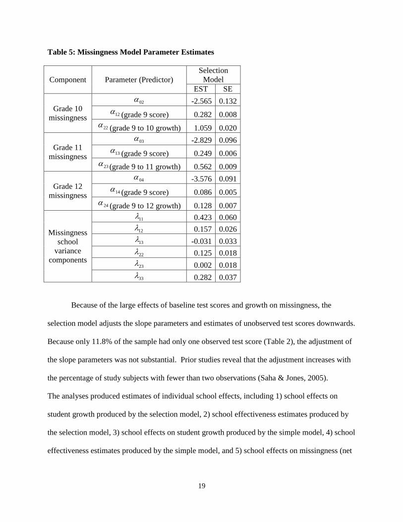
The parameter estimates for the missingness component of the selection model are

presented in Table 5. For each grade level with potential missingness, the baseline grade 9 test

score is predictive of missingness, as is the growth score. The effect of grade 9 test score is

largest for grade 10 missingness (estimate=0.282), followed by grade 11 missingness

(estimate=0.249), and then grade 12 missingness (estimate=0.086). Similarly, the effect of

growth score (growth from grade 9) is largest for grade 10 missingness (estimate=1.059,

standard error=0.020) and grade 11 missingness (estimate=0.562, standard error=0.009),

followed by grade 12 missingness (estimate=0.128, standard error=0.007). The effect sizes of

the predictors of missingness can be interpreted using odds ratios. For example, the odds of not

missing the grade 10 test increase by a factor of 1.335 for each 1-point increase in 9th grade

Composite score. The odds of not missing the grade 11 test increase by a factor of 1.75 for each

1-point increase in grade 9 to grade 11 growth.

3 This is calculated as 0.135*0.25 / 0.187 = 0.18. 4 This is calculated as 0.187*9 = 1.683 5 Calculated as exp(0.282)=1.33

19

Table 5: Missingness Model Parameter Estimates

Component Parameter (Predictor) Selection

Model EST SE

Grade 10 missingness

02α -2.565 0.132 12α (grade 9 score) 0.282 0.008

22α (grade 9 to 10 growth) 1.059 0.020

Grade 11 missingness

03α -2.829 0.096 13α (grade 9 score) 0.249 0.006

23α (grade 9 to 11 growth) 0.562 0.009

Grade 12 missingness

04α -3.576 0.091 14α (grade 9 score) 0.086 0.005

24α (grade 9 to 12 growth) 0.128 0.007

Missingness school

variance components

11λ 0.423 0.060 12λ 0.157 0.026 13λ -0.031 0.033 22λ 0.125 0.018 23λ 0.002 0.018 33λ 0.282 0.037

Because of the large effects of baseline test scores and growth on missingness, the

selection model adjusts the slope parameters and estimates of unobserved test scores downwards.

Because only 11.8% of the sample had only one observed test score (Table 2), the adjustment of

the slope parameters was not substantial. Prior studies reveal that the adjustment increases with

the percentage of study subjects with fewer than two observations (Saha & Jones, 2005).

The analyses produced estimates of individual school effects, including 1) school effects on

student growth produced by the selection model, 2) school effectiveness estimates produced by

the selection model, 3) school effects on student growth produced by the simple model, 4) school

effectiveness estimates produced by the simple model, and 5) school effects on missingness (net

20

of effects on test scores) for grades 10, 11, and 12. The intercorrelations of the school effects are

presented in Table 6.

Table 6: Correlations of School Effects Variable 1 2 3 4 5 6 7

1. School growth (selection model) 1.00 2. School effectiveness (selection model) 0.85 1.00 3. School growth (simple model) 0.99 0.84 1.00 4. School effectiveness (simple model) 0.84 0.98 0.85 1.00 5. Missingness - grade 10 -0.09 -0.12 -0.16 -0.21 1.00 6. Missingness - grade 11 -0.01 -0.07 -0.09 -0.17 0.83 1.00 7. Missingness - grade 12 0.26 0.12 0.25 0.11 -0.11 0.00 1.00 8. Proportion FRL-eligible -0.52 0.00 -0.52 0.00 -0.03 -0.10 -0.31

The correlation between the two school effectiveness measures from the two models is

0.98, suggesting that the selection model does not substantially change the rank ordering of

schools in terms of effects on student growth, adjusted for school poverty level. The correlation

between school effects on student growth and the school effectiveness measure is 0.85 for both

models. These high correlations indicate that adjusting for school poverty level makes a

difference in the rank ordering of schools. School poverty level had large negative correlations

with school growth for the selection model (R=-0.52) and for the simple model (R=-0.52),

showing that students enrolled at higher-poverty schools tend to experience less growth.

The correlations between school growth and school missingness effects were small in

magnitude with the exception of school effect on grade 12 missingness (R=0.26 for selection

model, R=0.25 for simple model). Higher missingness effects indicate that the school had less

missingness, so the positive correlation suggests that schools that have higher growth effects

have more students opting to test in grade 12, net of the effects of individual student test scores

and growth. School effects on grade 10 missingness were highly correlated with effects on grade

11 missingness (R=0.83), but neither was significantly correlated with grade 12 missingness. The

21

simple model’s estimates of school growth and effectiveness tended to have small negative

correlations with school effects on grade 10 and grade 11 missingness (correlations ranging from

-0.09 to -0.21). These correlations suggest that there is a weak negative relationship between

school growth effects and having fewer missed assessments, a direction that seems

counterintuitive. Similar findings were observed for the selection model.

Examples of estimates of high school mean growth and high school effectiveness (mean

growth adjusted for school poverty level) are provided in Table 7. Results for four high schools

are provided: a large school with high levels of missingness, a small school with high levels of

missingness, a large school with low missingness, and a small school with low missingness. In

each case, the mean growth estimates are lower under the selection model. This is expected

because the selection model acknowledges that students with lower growth are more likely to

have missing data. The differences between the selection and simple model are greater for the

two high schools (schools 4 and 78) with higher levels of missingness. For example, school 4 is

missing 25% of the grade 10 assessments, 27% of the grade 11 assessments, and 72% of the

grade 12 assessments. School 4’s mean growth estimate falls by 12.7% (from 0.181 to 0.158) by

moving from the simple model to the selection model. In contrast, school 126 is missing only

4% of the grade 10 assessments, 8% of the grade 11 assessments, and 75% of the grade 12

assessments. School 126’s mean growth estimate falls by only 1.6% (from 0.243 to 0.239) by

moving from the simple model to the selection model. Related to the changes in school mean

growth, the school effectiveness estimates are also impacted by model choice. School 4’s

effectiveness score drops from -0.011 for the simple model to -0.020 for the selection model.

School 126, on the other hand, sees an increase in its effectiveness score from 0.043 to 0.052.

22

Table 7: High School Effect Estimate Examples

High School

N Missingness Rates Measure Selection Model Simple Model

EST SE EST SE

4 457 25%, 27%, 72% Per-month growth 0.158 0.006 0.181 0.006 School effectiveness -0.020 0.008 -0.011 0.007

78 26 27%, 42%, 77% Per-month growth 0.110 0.022 0.138 0.021 School effectiveness -0.033 0.022 -0.020 0.021

126 613 4%, 8%, 75% Per-month growth 0.239 0.005 0.243 0.005 School effectiveness 0.052 0.007 0.043 0.007

209 35 3%, 11%, 89% Per-month growth 0.113 0.020 0.120 0.019 School effectiveness -0.026 0.021 -0.034 0.019

Estimates of individual student slope estimates were highly correlated (R=0.98) under the

two models. However, as was the case with the school effects, the results are different for

individual students when data are missing. In Table 8, the means and standard deviations of the

student slope estimates for the two models is presented for each missing data pattern. As

expected, the mean slopes are most similar when there are no missing data (pattern 8), with a

mean under the selection model of 0.204 and a mean under the simple model of 0.208. Under

the most common missing data pattern (pattern 5, missing only the grade 12 test), the models

also yield similar results (mean=0.178 under the selection model, 0.184 under the simple model).

Under the most extreme missing data pattern (pattern 1), the mean under the selection model was

substantially reduced to 0.064, compared to 0.135 under the simple model. For students who

missed both assessments after grade 10, the mean slope was 0.122 under the selection model and

0.136 under the simple model.

23

Table 8: Student Slope Estimate Summary Statistics, by Missing Data Patterns (O=test score missing, X=test score observed)

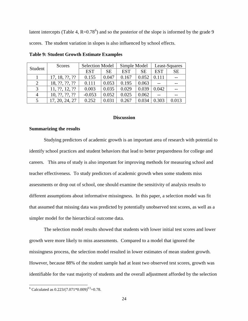
Examples of individual student growth estimates are provided in Table 9. Results for

five students with various missing data patterns are provided. Student 1 had observed scores for

grades 9 and 10, with a least-squares slope estimate of 0.111. The simple model’s estimate of

Student 1’s slope is 0.168, while the selection model’s estimate is 0.155. The simple model pulls

the least-squares estimate toward the school mean slope, while the selection model adjusts the

slope estimate downward because missed assessments are associated with lower growth.

Students 2 and 4 had just one observed score, which is the most severe case of missingness in

this study. It is therefore expected that the difference between the selection model estimate and

the simple model estimate will be most pronounced. Indeed, the growth estimate for Student 2 is

0.196 under the simple model, but falls to 0.111 under the selection model. The growth estimate

for Student 4 is 0.023 under the simple model, but falls to -0.053 under the selection model.

While the least-squares slope is not estimable for either student because there is just one data

point, the posterior mean growth estimates are much larger for Student 2 than for Student 4

under the simple model. This is the case because latent slopes are positively correlated with

Pattern Grade Level

% Selection model Simple Model

9 10 11 12 Mean SD Mean SD 1 X O O O 11.8 0.064 0.077 0.135 0.077 2 X X O O 8.3 0.122 0.081 0.136 0.074 3 X O X O 2.6 0.122 0.087 0.140 0.085 4 X O O X 0.0 0.100 0.067 0.113 0.066 5 X X X O 61.6 0.178 0.097 0.184 0.093 6 X X O X 0.6 0.106 0.072 0.111 0.070 7 X O X X 0.4 0.183 0.081 0.193 0.079 8 X X X X 14.7 0.204 0.083 0.208 0.080

24

latent intercepts (Table 4, R=0.786) and so the posterior of the slope is informed by the grade 9

scores. The student variation in slopes is also influenced by school effects.

Table 9: Student Growth Estimate Examples

Student Scores Selection Model Simple Model Least-Squares EST SE EST SE EST SE

1 17, 18, ??, ?? 0.155 0.047 0.167 0.052 0.111 -- 2 18, ??, ??, ?? 0.111 0.053 0.195 0.063 -- -- 3 11, ??, 12, ?? 0.003 0.035 0.029 0.039 0.042 -- 4 10, ??, ??, ?? -0.053 0.052 0.025 0.062 -- -- 5 17, 20, 24, 27 0.252 0.031 0.267 0.034 0.303 0.013

Discussion

Summarizing the results

Studying predictors of academic growth is an important area of research with potential to

identify school practices and student behaviors that lead to better preparedness for college and

careers. This area of study is also important for improving methods for measuring school and

teacher effectiveness. To study predictors of academic growth when some students miss

assessments or drop out of school, one should examine the sensitivity of analysis results to

different assumptions about informative missingness. In this paper, a selection model was fit

that assumed that missing data was predicted by potentially unobserved test scores, as well as a

simpler model for the hierarchical outcome data.

The selection model results showed that students with lower initial test scores and lower

growth were more likely to miss assessments. Compared to a model that ignored the

missingness process, the selection model resulted in lower estimates of mean student growth.

However, because 88% of the student sample had at least two observed test scores, growth was

identifiable for the vast majority of students and the overall adjustment afforded by the selection

6 Calculated as 0.223/(7.071*0.009)0.5=0.78.

25

model was modest. Importantly, our study did not include students missing baseline (grade 9)

test scores, and so additional missing data patterns were excluded. It is likely that including

students who did not have an observed grade 9 test score would have resulted in a greater

difference between the selection model results and those obtained from the simple model that

ignored the missing data process.

While the measures of school effectiveness were highly correlated for the selection model

and simple model (R=0.98), examination of school cases at the extremes of high and low

missingness illustrated that the school effect estimates can be sensitive to model choice.

Interestingly, school effects on missingness (net of the effects of test scores on missingness)

were not positively correlated with school effects on student growth.

Measures of student growth were also highly correlated under the simple model and selection

model. The selection model adjusted the mean student slope estimates downwards, and the

adjustment was very pronounced (52.9%, from a mean of 0.135 to a mean of 0.064) for students

who only had one observed test score. For other missing data patterns, the size of the adjustment

ranged from 2.1% to 12.9%.

Need for sensitivity analysis

While two models were considered, a more thorough analysis of the sensitivity of the

results to model choice would have considered a larger set of alternative selection models or

pattern-mixture models, both of which are designed to account for informative missingness. Our

selection model assumed that missingness depends on observed outcomes, whereas alternative

selection models, referred to as shared parameter models, might have assumed that missingness

depends on latent student or school variables, such as the student intercept and slope. The shared

parameter model assumes that latent student effects (e.g., true academic achievement or true

26

growth) affect missingness, whereas the selection model used in this study assumes that

potentially unobserved test scores affect missingness. The main distinction in the two

approaches is that the proposed selection model allows test score measurement errors to affect

missingness, whereas the shared parameter does not.

Pattern-mixture models, whereby separate estimates are derived for each possible missing

data pattern and then combined to form an overall estimate, could also be used in the sensitivity

analysis. MCMC model-fitting methods provide a flexible framework for conducting sensitivity

analysis because inferences can be made by simultaneously monitoring the posterior

distributions of functions of parameters from competing models.

Because proper prior distributions were specified for the variance-covariance matrices of

random effects, sensitivity to prior distributions was also checked. Priors were elicited from two

subject matter experts and the results under the set two sets of priors were virtually identical,

which was expected given the large sample of schools and students.

Model fitting using WinBUGS

The selection model and simple model were fit using the WinBUGS software. Flat priors

were specified for each parameter, with the exception of the three variance-covariance matrices

of random effects (student intercepts and slopes, school intercepts and slopes, and school

missingness effects). The prior distributions for the student and school effects were found using

a prior elicitation exercise with subject matter experts, while the prior distribution for the

variance-covariance of the school missingness effects was found using a data set independent of

the study data set. The prior distribution had effective sample sizes of 20, which is relatively

small compared to the sample size of 35,286 students and 223 schools.

27

The shared parameter model was relatively easy to fit using WinBUGS. Since

WinBUGS is currently free and accessible to everyone (see http://www.mrc-

bsu.cam.ac.uk/bugs), selection models can be implemented without much programming time and

without investing in special software. Since the missingness component of the selection model

adds considerable complexity to the posterior simulation, computing time is expected to be

significantly greater for the selection model relative to the simple model. For our data set of

35,286 students and 223 schools, WinBUGS required 2.5 seconds per iteration for

simultaneously fitting the selection model and simple model.

Limitations and ideas for additional research

As discussed earlier, only one selection model was examined whereas additional models

could have been fit to examine the sensitivity of the results to model specification. Student-level

predictors of achievement intercepts, achievement slopes, or missingness were not examined. It

is possible that the missingness process could have been explained by observable student

characteristics such as prior course grades, family income, psychosocial measures of motivation,

social engagement, and self-regulation (Casillas et al., 2012), and socio-demographic variables.

If the missingness process is completely explained by observed data, the test scores would have

been missing at random and there would be no need to fit the selection model. Future research

should examine predictors of test score intercepts and slopes, as well as the predictors of

missingness.

As discussed earlier, the primary distinction between the outcome-dependent missingness

model used in this study and a random-effects-dependent missingness is whether test score

measurement errors can affect the missingness process. Additional research should examine this

issue to determine if observed test scores or latent test scores are more predictive of missingness.

28

While our sample of high schools (N=223) and students (N=35,286) was quite large, it is

not necessarily representative of all schools in the United States. Schools had to have an all-

student testing program with ACT’s College Readiness Assessment System (ACT Explore, ACT

Plan, and the ACT college readiness assessment) to be included. School poverty level was

included as a predictor in the hierarchical growth model for test scores, and was shown to be

negatively related to both intercepts (grade 9 academic achievement) and slopes (academic

growth). Future research should include additional school characteristics as potential predictors

of academic growth and missingness.

The growth model assumed a common scale for the test scores and the school

effectiveness measure was defined as school mean slope, adjusted for school poverty level.

Alternative models that regress current test scores on prior test scores do not require or assume a

common scale of the test scores across multiple years (c.f., Allen, Bassiri, & Noble, 2009; Karl,

Yang, and Lohr, 2013). Future research should examine the appropriateness of using selection

models for growth models that assume common test score scales versus those that do not.

A final idea for future research would be to extend the high school growth model with

missingness to include college enrollment, college retention, and other college outcome data.

This research could examine effects of test score missingness, as well as academic achievement

status and growth, on future outcomes. The research could also extend the analysis of high

school effects on academic growth and missingness to include high school effects on college

enrollment and college outcomes.

29

References

ACT. (2013). ACT Plan Technical Manual. Iowa City, IA: Author.

Albert, P.S., & Follmann, D.A. (2000). Modeling repeated count data subject to informative

dropout. Biometrics, 56 (3), 667-677.

Allen, J., Bassiri, D., Noble, J. (2009). Statistical properties of accountability measures based on

ACT’s Educational Planning and Assessment System. ACT Research Report Series

2009-1, ACT, Inc.

Carlin, B.P. & Louis, T.A. (1996). Bayes and Empirical Bayes Methods for Data Analysis,

London: CRC Press, LLC.

Casillas, A., Robbins, S., Allen, J., Kuo, Y., Hanson, M. A., and Schmeiser, C. (2012).

Predicting early academic failure in high school from prior academic achievement,

psychosocial characteristics, and behavior. Journal of Educational Psychology, 104 (2):

407-420.

Diggle, P. & Kenward, M.G. (1994). Informative drop-out in longitudinal data-analysis. Applied

Statistics-Journal of the Royal Statistical Society Series C, 43, 49-93.

Feldman, B.J., Rabe-Hesketh, S.R. (2012). Modeling achievement trajectories when attrition is

informative. Journal of Educational and Behavioral Statistics. DOI:

10.3102/1076998612458701.

Geweke, J. (1992). Evaluating the accuracy of sampling-based approaches to the calculation of

posterior moments (with discussion), in Bayesian Statistics 4 (eds J.M. Bernado et al.),

Oxford University Press, Oxford, pp.169-93.

Hedeker, D. & Gibbons, R.D. (1997). Application of random-effects pattern-mixture models for

missing data in longitudinal studies. Psychological Methods, 2 (1), 64-78.

30

Hobert, J.P., & Casella, G. (1996). The effect of improper priors on Gibbs Sampling in

hierarchical linear mixed models. Journal of the American Statistical Association, 91

(436), 1461-1473.

Karl, A.T., Yang, Y., & Lohr, S.L. (2013). A correlated random effects model for nonignorable

missing data in value-added assessment of teacher effects. Journal of Educational and

Behavioral Statistics. DOI: 10.3102/1076998613494819.

Little, R.J.A. (1995). Modeling the drop-out mechanism in repeated measures studies. Journal of

the American Statistical Association, 90, 1112-1121.

McCaffrey, D.F., & Lockwood, J.R. (2011). Missing data in value-added modeling of teacher

effects. Annals of Applied Statistics, 5, 773-797.

Molenberghs, G., & Kenward, M.G. (2007). Missing data in clinical studies. West Sussex,

England: John Wiley.

Mori, M., Woolson, R.F., & Woodworth, G.G. (1994). Slope estimation in the presence of

informative right censoring - modeling the number of observations as a geometric

random variable. Biometrics, 50 (1), 39-50.

Pulkstenis, P., Ten Have T.R., & Landis, J.R. (1998). Model for the analysis of binary

longitudinal pain data subject to informative dropout through remedication. Journal of

the American Statistical Association, 93 (442), 438-450.

Raudenbush, S.W. & Bryk, A.S. (2002). Hierarchical Linear Models Applications and Data

Analysis Methods. Thousand Oaks, CA: Sage Publications.

Saha, C., & Jones, M.P. (2005). Asymptotic bias in the linear mixed effects model under non-

ignorable missing data mechanisms. Journal of the Royal Statistical Society, Series B, 67:

167-182.

31

Spiegelhalter, D., Thomas, A., Best, N., & Lunn, D. (2003). WinBUGS User Manual Version

1.4, January 2003. MRC Biostatistics Unit, Institute of Public Health. Cambridge, UK.

Tanaka, D., & Kanazawa, Y. (2010). Bayesian analysis of the latent growth model with dropout.

Department of Social Systems and Management Discussion Paper Series. University of

Tsukuba, Japan.

Wang, Y., & Taylor, J.M.G. (2001). Jointly modeling longitudinal and event time data with

application to acquired immunodeficiency syndrome. Journal of the American

Statistical Association, 96 (455), 895-905.

Wu, M.C., & Bailey, K. (1988). Analyzing changes in the presence of informative right

censoring caused by death and withdrawal. Statistics in Medicine, 7 (1-2), 337-346.

Wu, M.C. & Carroll, R.J. (1988). Estimation and comparison of changes in the presence of

informative right censoring by modeling the censoring process. Biometrics, 44 (1),

175-188.

Xu, S. & Blozis, S.A. (2011). Sensitivity analysis of mixed models for incomplete longitudinal

data. Journal of Educational and Behavioral Statistics. DOI:

10.3102/1076998610375836.

32

Appendix A: Prior elicitation exercise

Consider students who test with Explore at the start of grade 9, Plan in grade 10, the ACT in grade 11, and the ACT again (optionally) in grade 12. Think of their Composite scores plotted over time and summarized by an intercept and slope for each student. Assume that the average starting point is 16.0 and assume that the average yearly change in score is 1.2. Within the typical high school, starting true score varies by student. Assuming a 50th percentile score of 16, what do you think would be the 90th percentile starting true score? <P90_intercept entered as 21.00, 19.39> Within the typical high school, growth (average yearly true score change) varies by student. Assuming that the 50th percentile of true growth is 1.2, what do you think would be the 90th percentile of true growth? <P90_slope entered as 2.40, 1.79> What do you think would be the correlation of starting true score and true growth? <R_slope_intercept entered as 0.20, 0.27> True score starting points and true growth may also vary across high schools, after adjusting for school poverty level. Assuming a 50th percentile school-mean starting score of 16, what do you think would be the 90th percentile school-mean starting true score? < P90_school_intercept entered as 17.50, 18.31> Assuming a 50th percentile school-mean growth score of 1.2, what do you think would be the 90th percentile school-mean true growth score? <P90_school_slope entered as 1.60, 1.57> What do you think would be the school-level correlation of school-mean starting true score and school-mean true growth? <R_school_slope_intercept entered as 0.30, 0.32> The prior mean of the student and school covariance matrices is then calculated as:

Parameter Prior Mean Formula Prior Mean Expert #1

Prior Mean Expert #2

11Σ �𝑃90𝑖𝑖𝑖𝑖𝑖𝑖𝑖𝑖𝑖 − 16

1.645�2

9.24 4.25

12Σ 𝑅𝑠𝑠𝑠𝑖𝑖_𝑖𝑖𝑖𝑖𝑖𝑖𝑖𝑖𝑖� 11Σ 22Σ 0.049 0.022

22Σ �𝑃90𝑠𝑠𝑠𝑖𝑖 − 1.2

9 × 1.645�2

0.0066 0.0016

11η �𝑃90𝑠𝑖ℎ𝑠𝑠𝑠 𝑖𝑖𝑖𝑖𝑖𝑖𝑖𝑖𝑖 − 16

1.645�2

0.831 1.972

12η 𝑅𝑠𝑖ℎ𝑠𝑠𝑠_𝑠𝑠𝑠𝑖𝑖_𝑖𝑖𝑖𝑖𝑖𝑖𝑖𝑖𝑖� 11λ 22λ 0.0074 0.0112

22η �𝑃90𝑠𝑖ℎ𝑠𝑠𝑠 𝑠𝑠𝑠𝑖𝑖 − 1.2

9 × 1.645�2

0.00073 0.00062