A Beacon-Less Location Discovery Scheme

for Wireless Sensor Networks

Lei Fang (Syracuse)

Wenliang (Kevin) Du (Syracuse)

Peng Ning (North Carolina State)

Location Discovery in WSN

Sensor nodes need to find their locations Rescue missions Geographic routing protocols Many other applications

Constraints No GPS on sensors Cost must be low

Existing Positioning Schemes

Beacon Nodes

Two Important Elements

Reference points They must know their locations. e.g. beacon nodes, satellites.

Relationship between nodes and reference points Distance Angle of arrival Time of arrival Time difference of arrival

The Beacon-Less Scheme

Without using beacon nodes Beacon nodes are more expensive They can be the main target of attacks

Nonetheless, we still have to find reference points and the corresponding relationships. Remember: the locations of the reference points

must be known.

A Group-Based Deployment Scheme

A Group-Based Deployment Scheme

Modeling of The Group-Based Deployment Scheme

We still need another important element: The relationship between nodes and reference points.

Deployment Points:Their locations are known.

The Relationships

A

The Relationships

A

B

Modeling of the Deployment Distribution

Using pdf function to model the node distribution.

Example: two-dimensional Gaussian Distribution.

Other distribution can also be used.

The Idea

Observation at location O See more nodes from A and D

than from H and I.

Observation at location P Quit different from location O. See more nodes from H and I

than from A and D.

Given a location, we can derive the observation.

Given the observation, can we derive the location?

The Problem Formulation

Location θ = (x, y)

Observation a = (a1, a2, … an)

LocationEstimation

A Geometric Approach

Pick the three nearest deployment points (the three highest ai values).

Estimate the distance between the sensor and these points.

MLE (Maximum Likelihood Estimation):

f (Xi = ai | Z): The probability of observing ai nodes from Group i when the distance

is Z.

Find Z, such that f (Xi = ai | Z) is maximized.

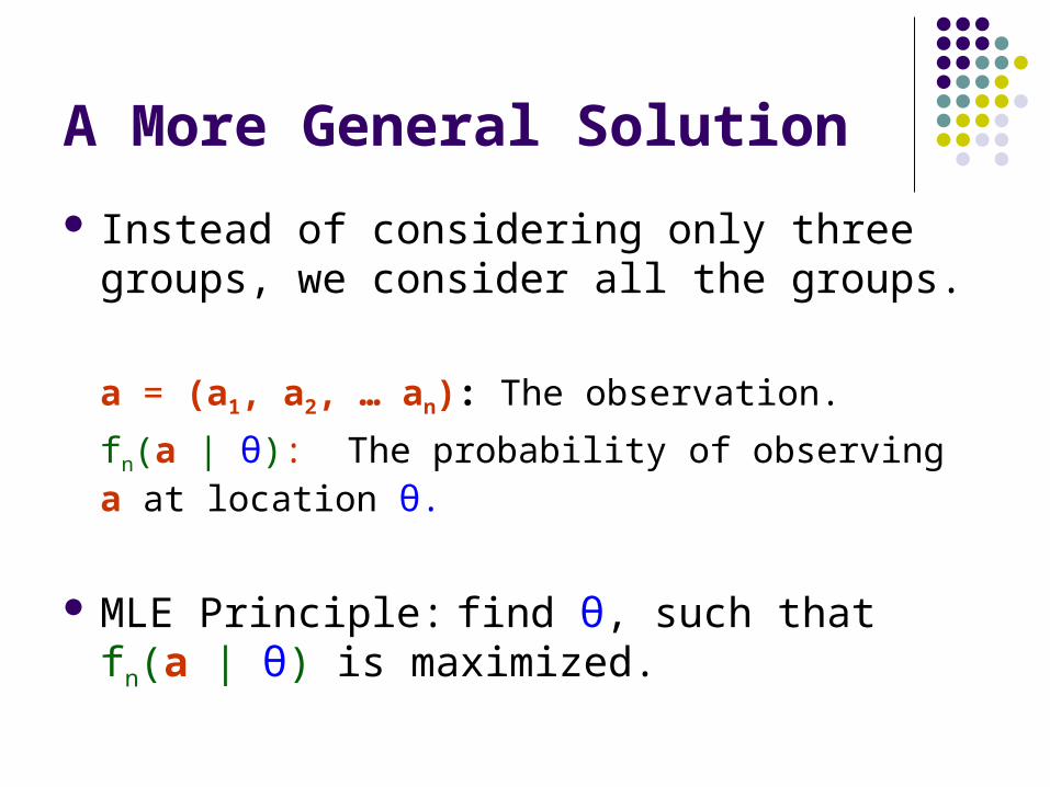
A More General Solution

Instead of considering only three groups, we consider all the groups.

a = (a1, a2, … an): The observation.

fn(a | θ): The probability of observing a at location θ.

MLE Principle: find θ, such that fn(a | θ) is maximized.

Maximum Likelihood Estimation

Likelihood Function fn(a | θ) = Pr (X1=a1, …, Xn=an | θ)

= Pr (X1=a1 | θ) · · · Pr (X1=an | θ)

L(θ) = log fn(a | θ)

Find θ:

0)(

0)(

y

L

x

L

Finding θ

Brute-Force Search: search all possible θ. Small Area Search:

Find an initial point (accuracy can be low). Conduct brute-force search around the initial point.

Gradient Descent: A standard solution.

Gradient Descent

A 2-dimensional function is represented as a surface in a 3-dimensional space

The maximum point (peak) holds a zero gradient

Find the shortest path to reach the peak. Could be expensive

Evaluation

Setup A square plane: 1000 meters by 1000 meters 10 by 10 grids (each is 100m X 100m) σ = 50 (Gaussian Distribution)

What to evaluate? Accuracy vs. Density Accuracy vs. Transmission Range Boundary Effects Computation Costs.

Effect of Density m

An Improvement:Dummy Nodes

m: number of sensors in each group

Effect of Transmission Range R

Effect of Boundary

Comparing the Three Numeric Approaches (Cost)

Comparing the Three Numeric Approaches (Accuracy)

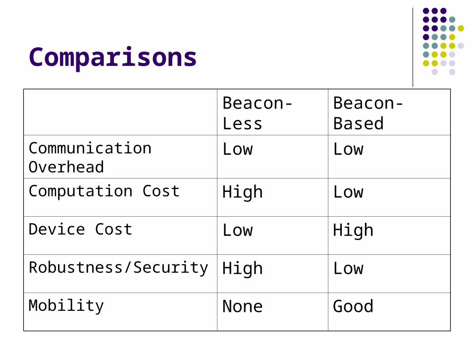
Comparisons

Beacon-Less Beacon-Based

Communication Overhead Low Low

Computation Cost High Low

Device Cost Low High

Robustness/Security High Low

Mobility None Good

Conclusion and Future Work

Beacon-Less Location Discovery Formulate the location discovery problem as an estimation

problem Use the Maximum Likelihood Estimation to solve the

estimation problem

Future work How the inaccuracy of the deployment model affect the

result? Resilience and Security:

IPDPS’05 paper (Best Paper Award in the Algorithm Track) Google “Wenliang Du” can get the paper.