A Brief Guide to Clinical Epidemiology

Written by Mac Students for Mac Students

Joanna Wielgosz Sean Kennedy Aashish Kalani Karman Chaudhry Staff Editor: Dr Haider Saeed

Table of Contents

Introduction

The Basics

Quantitative vs Qualitative

Variables

2x2 table

Collecting the Data

Sources of data

Surveillance systems and the physician’s role

Interpreting and Communicating the Data

Study Designs

Case-Control

Cohort

Cross Sectional

RCT

Analyzing the Data

Risks and Correlations

Relative Risk

Attributable Risk

Odds ratios

Correlations

Critical Appraisal

Sensitivity and Specificity

Predictive Values

Bias and Confounding

Reliability

Measures of Health and Disease

Incidence and Prevalence

Rates

Attack Rate

Case Fatality Rate

Answers to Practice Problems

Introduction

The McMaster Clinical Epidemiology Handbook has been designed by the Medical Education Interest Group in

collaboration with Dr. Haider Saeed. This handbook, initiated by the Medical Education Group, was part of an

initiative in the MD Program led by Dr. Saeed that was focussed on improving the Clinical Epidemiology

curriculum. The purpose of this handbook is to consolidate information provided by the core lectures in the

Clinical Epidemiology curriculum and provide clinical pearls and practice problems that enhance the applicability

of this information in a clinical setting. We encourage students to use this handbook longitudinally and revisit

topics throughout the Clinical Epidemiology curriculum, and beyond. The information in this handbook can also

be found online at www.mcmasterevidence.com where students in the MD program have actively helped

improve this resource, providing feedback and helping tailor the information for students.

We hope you find it useful.

The Basics

First off we’ll review some basics concepts of clinical epidemiology, providing a foundation before moving onto

some more specifics and clinical correlations.

Qualitative versus Quantitative

When performing tests and interpreting data, it is important to distinguish between qualitative versus quantitative measures. Qualitative, or categorical variables, are those that must be measured using a limited number of categories (e.g. a patient’s sex being male or female). Quantitative, or continuous variables, reflect a value that can lie anywhere along a scale (e.g. a patient’s weight in pounds). One should know whether the tests they are conducting give them qualitative or quantitative information. An important question to ask yourself is whether the information you get merely puts your patient into a broad risk category or provides a finite measurable value. We can explore this difference by looking at the results from a Urine Routine & Microscopy (R&M) ordered for a

patient. This test provides both qualitative and quantitative information to the clinician. The dipstick portion of

the test can provide binary or qualitative information. One use of the test is to provide the clinician with a sense

of how many leukocytes are in the urine (a sensitive marker of a UTI… we’ll get to that later). This is presented

as a qualitative measure. You can either have none, 1+, 2+ or 3+ leukocytes in the urine. On the other hand,

urine pH (a marker of toxin ingestion and kidney disease among others) is a quantitative parameter since pH is

measured on a scale of 1-7.

While it may seem that quantitative variables can provide the clinician with more precise information, this does

not always speak of its clinical utility. On the one hand, a positive urine glucose is a useful marker of diabetic

nephropathy - a specific measure of the exact quantity of glucose in the urine is not needed. Nevertheless, in the

case of positive epithelial cells in the urine sample, this may indicate pathology or a poorly obtained sample -

here, perhaps the information provided as a quantitative measure would be more useful.

Independent versus Dependent Variables

A dependent variable is self-explanatory; it is dependent on the variation of another factor (you guessed it, the

independent variable). In general, we manipulate independent variables in order to see a change in dependent

variables. This concept is best explained through an example: The partial pressure of oxygen decreases with

increasing altitude. Here, PO2 is dependent on the changing altitude.

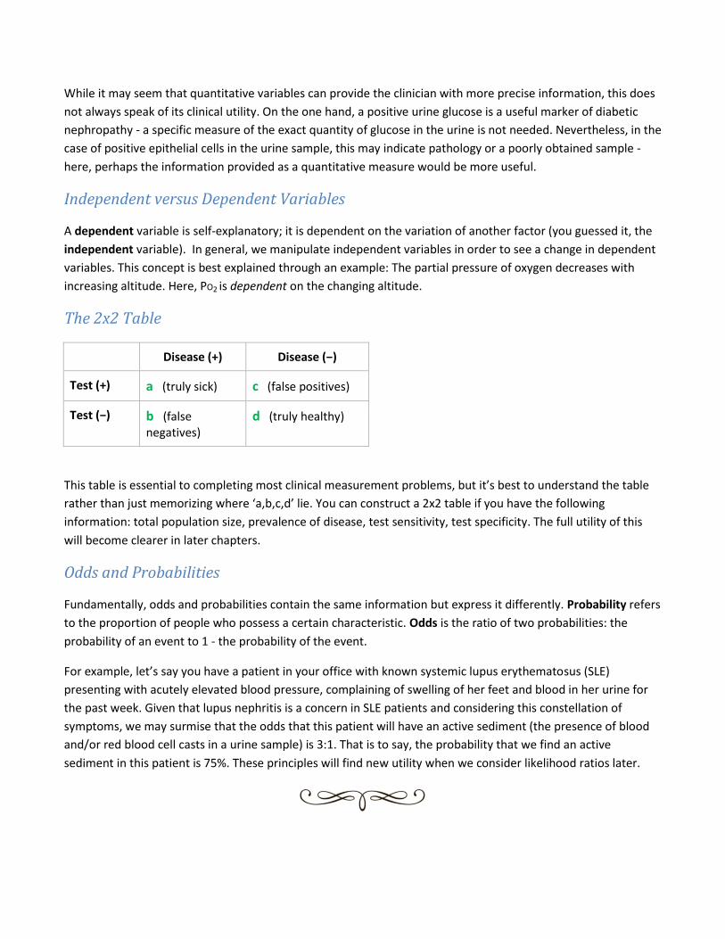
The 2x2 Table

Disease (+) Disease (−)

Test (+) a (truly sick) c (false positives)

Test (−) b (false negatives)

d (truly healthy)

This table is essential to completing most clinical measurement problems, but it’s best to understand the table

rather than just memorizing where ‘a,b,c,d’ lie. You can construct a 2x2 table if you have the following

information: total population size, prevalence of disease, test sensitivity, test specificity. The full utility of this

will become clearer in later chapters.

Odds and Probabilities

Fundamentally, odds and probabilities contain the same information but express it differently. Probability refers

to the proportion of people who possess a certain characteristic. Odds is the ratio of two probabilities: the

probability of an event to 1 - the probability of the event.

For example, let’s say you have a patient in your office with known systemic lupus erythematosus (SLE)

presenting with acutely elevated blood pressure, complaining of swelling of her feet and blood in her urine for

the past week. Given that lupus nephritis is a concern in SLE patients and considering this constellation of

symptoms, we may surmise that the odds that this patient will have an active sediment (the presence of blood

and/or red blood cell casts in a urine sample) is 3:1. That is to say, the probability that we find an active

sediment in this patient is 75%. These principles will find new utility when we consider likelihood ratios later.

Collecting the Data

Sources of Data

Proper collection of data is essential to producing meaningful and valid results and therefore cannot be done

haphazardly. In turn, when reading results (e.g. efficacy of a certain drug) it is important to consider who was

being studied - were the subjects chosen from a heterogenous population like the entirety of Hamilton or a

smaller, healthier sub-population such as a McMaster campus?

Principles of Sampling

Ask yourself…. Who? (inclusion/exclusion, representation of population of interest) How? (which sampling method) How many? (will give you statistical power, limits of funding)

Non-probability sampling

This type of sampling assumes equal distribution of characteristics among a population. It does not allow for

recognition of any sampling variability or bias is present.

Convenience: sampling units chosen because they’re easy to get

Judgment: Investigator chooses what he deems to be representative units of source pop

Purposive: sampling units chosen on purpose because of exposure/disease status (e.g. patients with T2DM in

evaluation of ramipril for blood pressure control)

Pros: relatively easy, cheaper, good for homogenous populations

Cons: biased results if not representative, limited extrapolation

Probability sampling (random selection)

Simple random sampling: A sample is chosen from a population where all have equal chance of being included.

One must have a list of all units in a population. Essentially a lottery method.

Systematic random sampling: a population is divided into intervals and then a random starting point is chosen.

E.g. A pool of 1000 hospital patients is to be sampled from. Dividing the population of 1,000 by 50 yields 20

intervals. Thus, each 20th patient is chosen, beginning with a random starting point between 1 and 20. If 4 is

chosen as the random starting point, invoices selected will be 4, 24, 44, 64, and so on.

Stratified random sampling: Before choosing units, sampling frame broken down into strata based on some

factor likely to influence the level of the characteristic being measured (e.g. gender). Then, simple random

sampling conducted within each strata.

Pros: provide most credible results

Cons: time consuming, difficult to obtain list of entire population

Others

Cluster: Sampling unit is a group of individuals with things in common, but unit of concern still individual. (Note:

All individuals in cluster tested). An example of a cluster may be a geographic location such as districts in

Hamilton ON.

Multistage: Sampling takes place both at cluster/group level and individual level. Convenient when too many

individuals in a cluster to obtain measurements from and when individuals in cluster are very alike (e.g.

purebred puppies).

Pros: cost effective

Cons: less efficient, less control over final sample size

Surveillance Systems

Disease surveillance allows us to estimate incidence and prevalence of both acute infectious disease as well as

chronic conditions. It is important for outbreak planning as well as resource allocation, as we can project future

healthcare needs based upon trends seen by surveillance. As physicians, we will utilize information about

prevalence and incidence to aid in diagnosis and will be often be required to report certain diseases to public

health.

Surveillance systems allow for a coordinated effort between local, provincial and federal systems. The integrity

of confidentiality of patient information must be maintained while still allowing for notification of affected

persons.

Key players: CDC (Centre for Disease Control) in the United States, PHAC (Public Health Agency of Canada)

Some of the current monitoring systems in place:

1. Reportable diseases - e.g C. Trachomatis, Tuberculosis, Hepatitis A/B/C [Source: physician and self-reporting]

2. Annual monitoring - West Nile, Influenza (“Flu Watch”) [Source: physician/hospital reporting]

3. The Canadian Chronic Disease Surveillance System (CCDSS) [Source: administrative databases including physician billing, hospitalization and resident registry databases]

Interpreting and Communicating the Data

Study Designs

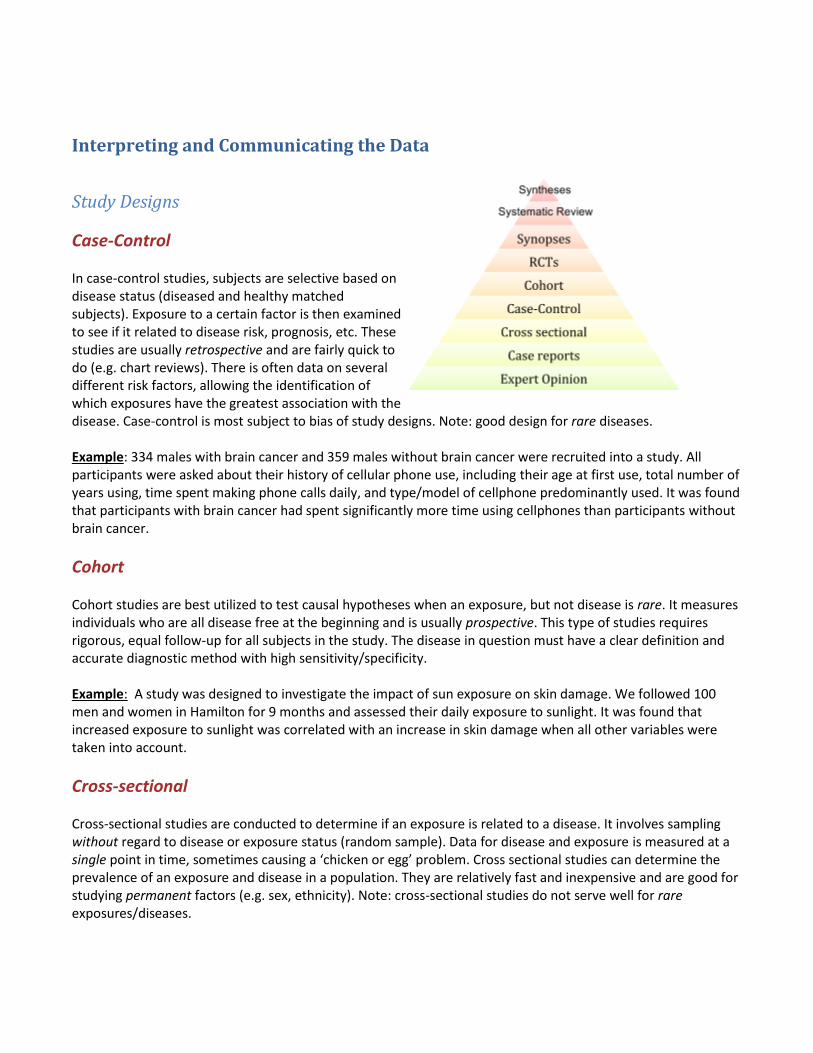
Case-Control In case-control studies, subjects are selective based on disease status (diseased and healthy matched subjects). Exposure to a certain factor is then examined to see if it related to disease risk, prognosis, etc. These studies are usually retrospective and are fairly quick to do (e.g. chart reviews). There is often data on several different risk factors, allowing the identification of which exposures have the greatest association with the disease. Case-control is most subject to bias of study designs. Note: good design for rare diseases. Example: 334 males with brain cancer and 359 males without brain cancer were recruited into a study. All participants were asked about their history of cellular phone use, including their age at first use, total number of years using, time spent making phone calls daily, and type/model of cellphone predominantly used. It was found that participants with brain cancer had spent significantly more time using cellphones than participants without brain cancer.

Cohort

Cohort studies are best utilized to test causal hypotheses when an exposure, but not disease is rare. It measures individuals who are all disease free at the beginning and is usually prospective. This type of studies requires rigorous, equal follow-up for all subjects in the study. The disease in question must have a clear definition and accurate diagnostic method with high sensitivity/specificity. Example: A study was designed to investigate the impact of sun exposure on skin damage. We followed 100 men and women in Hamilton for 9 months and assessed their daily exposure to sunlight. It was found that increased exposure to sunlight was correlated with an increase in skin damage when all other variables were taken into account.

Cross-sectional Cross-sectional studies are conducted to determine if an exposure is related to a disease. It involves sampling without regard to disease or exposure status (random sample). Data for disease and exposure is measured at a single point in time, sometimes causing a ‘chicken or egg’ problem. Cross sectional studies can determine the prevalence of an exposure and disease in a population. They are relatively fast and inexpensive and are good for studying permanent factors (e.g. sex, ethnicity). Note: cross-sectional studies do not serve well for rare exposures/diseases.

Example: 15356 males and females were polled and asked about their height/weight ratio and the number of hours spent watching television each week. It was found that there was a negative correlation between height/weight ratio and number of hours spent watching television per week.

Randomized Controlled Trials (RCTs) Randomized controlled trials are the gold standard in clinical trials. RCTs can be used to test the efficacy of an

intervention in a population by comparing two randomly assigned groups; one that receives the intervention

and one that does not. The group that does not receive intervention may receive a placebo or sham procedure.

For obvious ethical reasons, standard of care known beneficial therapies must be used in the non-intervention

group.

Often times the patient group that does not receive intervention is blinded to this fact (“single blind”). In this

case they may receive a placebo or have a sham procedure performed. Additionally, some RCTs may blind

physicians and even data analysts/researchers to which patient group is receiving the intervention.

Example: 12000 adults with hypertension (>140/90) were randomized to two groups; 6000 received an ACE

inhibitor and a placebo pill and 6000 received an ACE inhibitor combined with a diuretic. Neither patients nor

clinicians knew which group was allocated which drugs. At 1 year followup, the ACE inhibitor combined with a

diuretic group had significantly lower blood pressure.

Analyzing the Data

Risks and Correlations

Relative Risk

Relative risk if defined as the ratio between risk of disease in exposed and the risk of disease in unexposed. A larger relative risk points to a stronger association between exposure and disease. Note: relative risk is not applicable to case-control studies.

Attributable Risk

Attributable risk measures the additional risk of disease in those exposed as compared to the unexposed. In other words, it reflects the proportion of disease occurrences that are attributable to a certain exposure. When considering attributable risk, one must take into account the background incidence of disease in a population (i.e. the prevalence of disease that may be caused by other reasons than the exposure in question). Attributable risk can be easily determined from cohort studies, which provide information on both exposure and disease status. It is useful when researchers want to identify how much a disease can be prevented. Example: For example, let’s say a study showed that the incidence of lung cancer is higher in adults who lived in the

homes of smoking parents versus not, accounting for smoking habits of the subjects themselves and work exposures (baseline risk). 300 subjects were exposed to second-hand smoke and 300 were not. 10/300 second-hand smoke subjects developed lung cancer while 2/300 in the unexposed developed the disease. Therefore, the attributable risk would be ([10-2]/300 = 8/300 = 2.7%). Calculation: AR is determined by subtracting disease incidence in those unexposed from those exposed. Attack rate = incidence dx (exposed) - incidence dx (unexposed)

Odds Ratios

This is the ratio of the odds of developing a condition or disease among those exposed to a risk factor to those who are not exposed.

Example: Suppose we have a town of 200 people. In this town 100 people are exposed to asbestos and 80 of those exposed develop mesothelioma. Therefore, the probability of developing mesothelioma is 80/100=0.8 in those exposed to asbestos. In the 100 people in the town not exposed to asbestos, only 1 individual develops mesothelioma. The probability of developing mesothelioma is 1/100=0.01 in those not exposed to asbestos. The odds ratio is is the probability of developing mesothelioma in those exposed to asbestos divided by the probability of developing mesothelioma without asbestos exposure. Therefore, odds ratio=0.8/0.01= 80. Calculation: OR = probability dx (exposed)/probability dx (unexposed) In a 2x2 table, OR can be calculated as: OR = (a × d)/(b × c)

Interpreting the odds ratio:

The odds ratio can give us a measure of how strongly the risk factor is associated with the outcome.

If the OR is > 1, the control is better than the intervention.

If the OR is < 1, the intervention is better than the control.

Critical Appraisal

Sensitivity and Specificity

Sensitivity is defined as the proportion of individuals that actually HAVE the disease and

test POSITIVE. This measurement gave give us insight into false negatives of a test (1-Sn);

if a test is highly sensitive and you obtain a negative result, you can be confident in ruling

the disease out (SnOUT).

Specificity in contrast reflects the proportion of individuals that DON’T have the disease

and test NEGATIVE. This gives us information into false positives of a test (1-Sp); if a test is

highly specific and you obtain a positive result, you can be confident in ruling the disease

in (SpIN).

The 2x2 Table:

Disease (+) Disease (−)

Test (+) a (truly sick) c (false positives)

Test (−) b (false negatives)

d (truly healthy)

Calculations:

In a 2x2 table, it can be calculated as: Sensitivity = a/(a+c)

In a 2x2 table, it can be calculated as: Specificity = d/(b+d)

Example:

Suppose that in patients with acute CHF, the complaint of dyspnea upon exertion had a sensitivity of 100% and a

specificity of 17%. With such a high sensitivity, we would make the assumption that if a patient does not have

dyspnea on exertion, this patient does not have acute CHF (remember SNout – high SeNsitivity allows us to rule

OUT, and vice versa). However, with such a poor specificity, we cannot assume that a patient complaining of

dyspnea on exertion is definitively having acute CHF—they may be having one of the many other causes of

dyspnea (remember SPin – a high specificity allows us to rule in, and vice versa).

Practice Problem:

2. Below are the hypothetical results of women who have had a mammogram:

Breast cancer No Breast Cancer

(-) mammogram 30 720

(+) mammogram 70 180

Q: What is the specificity and the sensitivity of the mammogram?

Predictive Values

Predictive values answer the following question: What is the probability of disease given the test result? Positive predictive value (PPV) reflects the proportion of test POSITIVES that are truly DISEASED. Negative predictive value (NPV) reflects the proportion of test NEGATIVES that are truly HEALTHY. These values are affected by prevalence and so are not clinically useful as sensitivity and specificity (but will still be on exams so learn them!). Why does dependent on prevalence matter? It means NPV and PPV are dependent on the population a patient is drawn from. For example, the PPV of an elevated troponin related to a myocardial infarction increases if a patient presents with concurrently with chest pain and diaphoresis. It increases because the population from which the patient is drawn is different (from a general population with a low prevalence of MI to a clinically suspicious population with a much higher prevalence). Calculations:

PPV = true positives/total positives NPV = true negatives/total negatives False positives = 1 – PPV False negatives = 1 – NPV Practice Problem: 1. A colonoscopy can test for cancer, and it has a sensitivity of 75%, and a specificity of 67%. The positive predictive value (PPV) of this test is about ___ and the negative predictive value (NPV) is about ___:

Colon Cancer No Colon Cancer

(+) test 30 20

(-) test 10 40

a) 60%, 80% b) 99%, 65% c) 75%, 67% d) 17%, 80%

Likelihood Ratios

The likelihood ratio (LR) reflects how likely a particular test result is in a patient with a disease in question versus

one without said disease. It combines sensitivity and specificity to apply a test result to an individual patient. A

positive likelihood ratio is how much a positive test increases the chance of that patient having the disease. A

negative LR on the other hand is how much a negative result decreases the chance of the patient having the

disease.

LR+ is the same as the probability of true positives divided by the probability of false positives.

LR- is the same as the probability of false negatives divided by the probability of true negatives.

Pre-test Probability

Pre-test probability is defined as the probability of a condition being present BEFORE a diagnostic test is performed. There are two ways we can determine the pre-test probability:

1. Approximation based on previous clinical experience. Ie. In your experience, how often do patients you see have cholecystitis when they present with RUQ pain. Approximation is vulnerable to random error and bias.

2. Looking at EBM literature where pre-test probabilities have been determined for a wide variety of conditions.

Post-test Probability

Post-test probability is defined as the probability of a condition being present after a diagnostic test. Ideally, your goal is to order diagnostic tests that make post-test probability SIGNIFICANTLY HIGHER OR LOWER in order to get closer to definitively ruling in or ruling out a condition.

Interpreting Likelihood Ratios:

Diagnostic tests with LR+s (all LRs>1) increase the likelihood of a condition being present.

Diagnostic tests with LR-s (all LRS<1) decrease the likelihood of a condition being present.

Above 10 represents a diagnostic test that of strong value and can often definitively rule in a condition.

Between 2 and 10 represents a diagnostic test that is of moderate value (it helps to increase probability of a condition but often does not definitively rule it in).

Between 1 and 2 represents a diagnostic test that is useless in terms of ruling in a condition.

Between 0.5 and 1 represents a diagnostic test that is useless in terms of ruling out a condition.

Between 0.1 and 0.5

represents a diagnostic test that is moderately useful in ruling out a condition (it helps to decreases probability of condition but often does not definitively rule it out).

Less than 0.1 represents a diagnostic test that is of strong value and can often definitively rule out a condition.

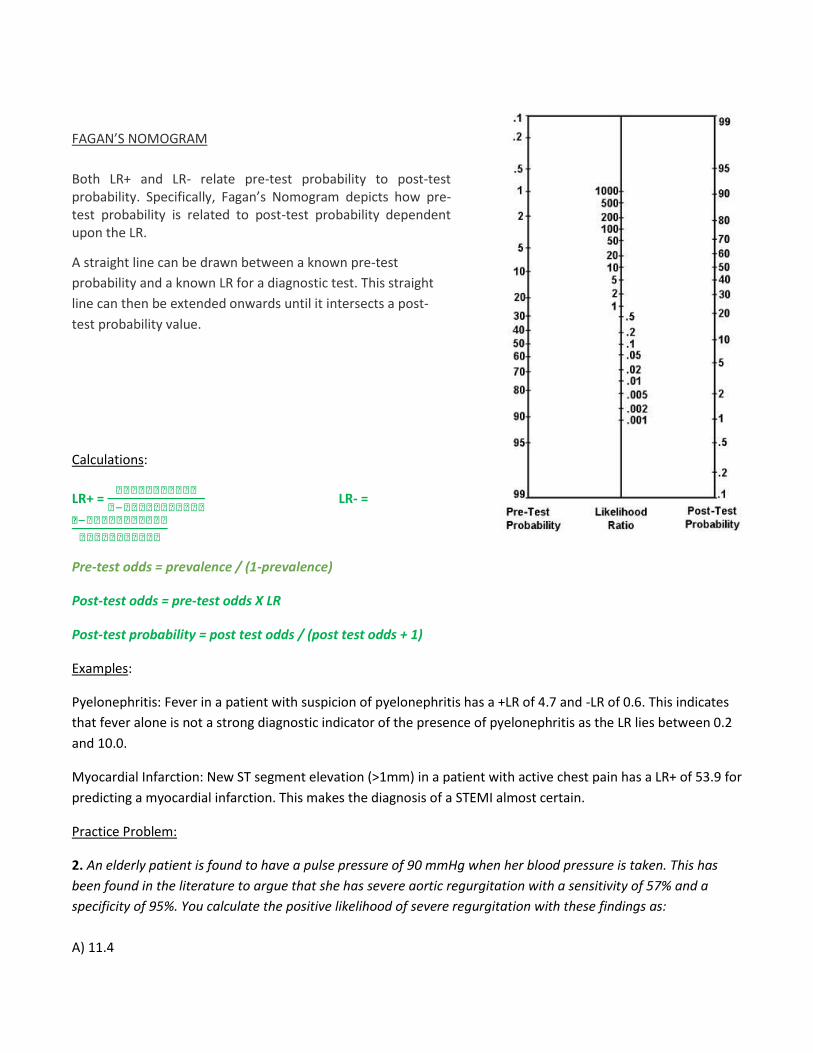
FAGAN’S NOMOGRAM

Both LR+ and LR- relate pre-test probability to post-test probability. Specifically, Fagan’s Nomogram depicts how pre-test probability is related to post-test probability dependent upon the LR.

A straight line can be drawn between a known pre-test

probability and a known LR for a diagnostic test. This straight

line can then be extended onwards until it intersects a post-

test probability value.

Calculations:

LR+ =

LR- =

Pre-test odds = prevalence / (1-prevalence)

Post-test odds = pre-test odds X LR

Post-test probability = post test odds / (post test odds + 1)

Examples:

Pyelonephritis: Fever in a patient with suspicion of pyelonephritis has a +LR of 4.7 and -LR of 0.6. This indicates

that fever alone is not a strong diagnostic indicator of the presence of pyelonephritis as the LR lies between 0.2

and 10.0.

Myocardial Infarction: New ST segment elevation (>1mm) in a patient with active chest pain has a LR+ of 53.9 for

predicting a myocardial infarction. This makes the diagnosis of a STEMI almost certain.

Practice Problem:

2. An elderly patient is found to have a pulse pressure of 90 mmHg when her blood pressure is taken. This has

been found in the literature to argue that she has severe aortic regurgitation with a sensitivity of 57% and a

specificity of 95%. You calculate the positive likelihood of severe regurgitation with these findings as:

A) 11.4

B) 1.4

C) 4.3

D) 0.45

E) 0.6

Bias

Bias is any systematic error in the design, conduct or analysis of a study that causes an incorrect estimate of an

exposure’s influence on disease risk.

Types of biases include:

1. Selection Bias

(a) Non-response bias: occurs low response rate/ volunteer bias. Bias due to differences in characteristics

between participants and opt-outs.

(b) Loss to follow-up: difference between true value and the observed in a study due to characteristics of

those who choose to withdraw

(c) Healthy-worker effect: workers who suffer from symptoms might die, retire and those that remain appear

to be healthy group of people

Control above by paying attention to study design

2. Information Bias

(a) Misclassification: error in obtaining and classifying info and can affect classification of disease/exposure.

Can be due to inaccurate diagnostic tests, a poor questionnaire, non-compliance in randomized clinical trial or

interviewer bias (leading questions).

(b) Non-differential: error not related to exposure or outcome – inherent problem with data collection

methods

(c) Differential: rate of misclassification differs between cases and controls or between exposed/unexposed

(d) Recall: systematic error due to differences in accuracy/completeness of recall to memory

(e) Wish: cases may seek to show that disease isn’t their fault (e.g. deny smoking)

(f) Surrogate: rely on family members for information (E.g. for a child, patient with dementia)

Confounding

Confounding is also a type of bias. It occurs when the observed association between an exposure and outcome

is mixed up with a third factor. We might think we are measuring the association of an exposure factor with an outcome, but the association measure also includes the effects of one or more extraneous factors. To a confounder, the factor must be:

1. Associated with the disease (outcome) 2. Associated with the exposure 3. Not a consequence of exposure

The third point above alludes to the idea of mediators, which are intervening variables or parts of the causal

pathway. An example of this is seen with multiple sexual partners, increased risk of HPV infection, and cervical

cancer. Having multiple sexual partners causes cervical cancer through the intermediate step of increasing an

individual’s risk for HPV infection.

We can control for confounding in the design stage of a study (through randomization, restriction/exclusion,

matching) and/or during the analysis stage (through stratification, multivariable modeling).

Example: 12000 adults with hypertension (>140/90) were randomized to two groups; 6000 received an ACE inhibitor and a placebo pill and 6000 received an ACE inhibitor combined with a diuretic. Neither patients nor clinicians knew which group was allocated which drugs. At 1 year followup, the combined diuretic/ACE inhibitor group had significantly lower blood pressure. Unfortunately, the study coordinators did not randomize genders and age groups adequately. The combined diuretic/ACE inhibitor group had significantly younger population and more females. Consequentially, gender and age are potential confounders in the outcome of this study.

Reliability

Inter or intra-rater reliability is most often determined by a statistical measure known as Kappa. Kappa measures rater agreement beyond what would be due to chance alone (expected agreement). Values <0.2 show slight agreement and those >0.8 have excellent agreement.

Measures of Health and Disease

Prevalence and Incidence

Prevalence is defined as the number of existing cases of disease in a population at a certain point in time. It is a unitless proportion that does not take into account when a disease happened (i.e. measures both old and new cases). Therefore, it must not be interpreted as a measure of disease risk (no account for duration of disease).

This measure works best for diseases of long duration. Incidence in contrast is a dynamic measure of disease occurrence that reflects new disease occurrence over a period of time. It is expressed in term of disease risk (likelihood an individual will contract the disease of interest). Incidence requires two measurements: those who are disease free and those have become diseased since. This measure works best for diseases of short duration. Example: As of 2014, 20% of population X is obese (prevalence=20%) . Unfortunately, 5% of

population X is becoming newly obese annually (incidence=5%).

Practice Problem: 3. A new treatment is developed that prevents death but does not produce recovery from disease. Q: Which of the following will occur? A. Prevalence will increase B. Prevalence will decrease C. Incidence will increase D. Incidence will decrease E. None of the above

Rates

Case fatality rate

This reflects the number of individuals that died from a disease out of the total number of individuals with the disease. This measure can be used as a way to determine prognosis for those with a certain disease/illness. It is commonly used for diseases with limited courses (e.g. meningococcal disease). Calculation:

CFR =

(during a specified time period)

Practice Problem: 4. C. difficile infection is a growing problem in inpatient healthcare facilities. An outbreak of C. difficile in 33 hospital patients during the month of July caused 4 disease-related deaths. What is the case fatality rate?

Attack Rate

This is defined as the number exposed who became ill out of the total number exposed. These are generally

calculated for limited periods of time, such as an epidemic. Calculation:

AR =

(during a specified time period)

Practice Problem: 5. In a preschool class of 30 children, 2 girls and 1 boy have contracted a cold virus. Over the next two weeks, 2 more boys and 3 more girls develop similar symptoms. Q: What is the attack rate?

Answers to Practice Problems

1. Specificity= 72%, Sensitivity=70%

2. A

3. A

4. (CFR) 4/33 = 12%

5. (AR) Three already have condition as a results. 30-3=27. 27 still at risk and 5 develop. Therefore, attack rate is

5/27= 18.5%.