1

Department of Economics, University of Umeå

July 2011 revised March 2014.

A Brief History of Envelope Theorems in Economics: Static and Dynamic

By Karl-Gustaf Löfgren1

Abstract: This paper studies how envelope theorems have been used in Economics, their

history and also who first introduced them. The existing literature is full of them and the

reason is that most families of optimal value functions can produce them. The paper is

driven by curiosity, but hopefully it will give the reader some new insights.

Keywords: Envelope theorems, names and history, value functions and cost-benefit

analyses.

JEL-Codes: B16, B 21, B40

1. Introduction

Given that what we know about envelope theorems today in economics the (engineering)

proofs are not difficult, but this was not true at the time they were known in economics

from result by among others Hotelling (1932), Roy (1947) and Shephard (1953). It is obvious

how Roy and Shephard came up with their results, but I used to tell graduate students that I

will let them pass the microeconomics exam if they can find Hotelling’s lemma in his article

from (1932)2. The results may be viewed as corollaries of a general envelope theorem

produced in mathematics. Mathematically an envelope is (loosely) defined as a curve that is

touched by all members of a family of curves. There are theorems that in calculus give

conditions for the existence of envelops to families of curves.

1 With assistance from Professor Erwin Diewert. Professor Thomas Aronsson Department of Economics, Umeå University and Professor Rolf Färe, Department of Economics, Oregon University, Corvallis commented previous versions of the document. They certainly improved the paper. 2 The result can be found on page 22 in this paper..Paul Samuelson (1947) cites Hotelling (1932) without mentioning his “envelope result”. This indicates that it may be a two pipe problem.

2

Some of the first envelope theorems produced by pure mathematicians may have been

introduced by Ernst Zermelo (1894), Jean Darboux (1894) and Adolf Kneser (1898). They

produced them in connection with new results in the calculus of variations.

The envelope theorem in calculus stands on its own, but the geometry is interesting for

economic theory. It is well known that economists like Jacob Viner (1931), Roy Harrod (1931)

and Erich Schneider (1931) used envelope properties to discuss the connection between

short run and long run cost curves. Paul Samuelson (1947) derives the formal general proof

of what today is called an envelope theorem, but under the headline “Displacement of

Quantity Maximized”3. He mentions Viner’s application of it as an example. Viner had a

draftsman that produced his graph called Dr Wong. He insisted on tangency between the

long run envelope cost curve and the short run curve, and he was right. However, he was not

able to convince Viner. This means that there is a well- known error where a falling long run

cost curve passes through the minimum of a short run cost curve.

Samuelson probably believed, at the time he produced his version of the envelope theorem,

that he was the first to show what the second order change looked like, how the difference

between the full second order change with respect to a parameter looked like in relation to

the partial second order change, and how this difference could be signed by using the

second order conditions (a negative semi-definite quadratic form for maximum). The last

result is the only one that was new.

The first results in economics 4 on “comparative dynamics” in optimal control I have seen are

available in a deep, not easy to read, paper by Oniki (1973), and they are based on the

assumptions concerning the optimal control as a function of parameters. A proof of a special

case appears in Benveniste and Scheinkman (1979). Seierstad (1981, 1982) proved under

what conditions the (sub)-derivatives of the optimal value function exist and what they look

like with respect to changes in the initial and final conditions and changes in parameters.

3 Samuelson (1947) pp 34-35. 4 There is also a result by Arrow in Arrow and Kurz (1970) based on dynamic programming that shows that the derivative of the value function with respect to initial conditions, calculated along an optimal path, is the adjoint function of the maximum principle.

3

When concavity is added, sub-derivatives change to derivatives. Slightly more general

results were produced by Malanowski5in (1984).

There are also, eight and nine years later, two papers in the same journal as Seierstad’s

(1982) paper on derivatives of the value function with respect to parameters. The papers are

written by Caputo (1990b) and La France and Barney (1991). They contain similar stuff

although Seierstad’s paper is the more stringent. Unlike Caputo and La France and Barney,

Seierstad did not focus on derivatives with respect to parameters, but as we will see below

parameters can be looked upon as “petrified” state variables.

With respect to the Calculus of Variations Caputo (1990a) has also contributed a paper on

comparative dynamics via envelope methods. I am not sure that there exist many similar

papers in the literature, but there exist a similar envelope result in my lecture notes that was

copied from lectures by my teacher Tönu Puiu in the late seventies. Caputo seems,

however, not to have seen Seierstad and Sydsaeter (1987) who have contributed with

complete proofs of the differentiability of the optimal value function with respect to initial

and final conditions and endpoint time6.

2. The Austrian outlaws and the envelope theorem in economics

In this section, we will show how the envelope theorem may first have been introduced by

economists rather than pure mathematicians. The two who did it were two Austrian cousins,

Rudolp Auspitz and Richard Lieben, who, as Niehans (1990) writes,” succeeded where

Menger had failed, namely in providing the theory of price with an analytical apparatus”.

Both cousins were born in Vienna and both died there, but none of them belonged to the

Viennese School which was dominated by among others Carl Menger, Eugen von Böhm-

Bawerk , Fridriech Wieser and Gustav Schmoller. While Menger and others were occupied

by “Der Metodenstreit”, the outsiders Auzspitz and Lieben produced the only Austrian 19;th

century contribution to mathematical economics; one of the outstanding contributions

during the last two decades of the century . Both of them had studied mathematics. Auspitz

did not finish his degree. He moved into business and founded one of the first sugar

5 See also the references therein. 6 See Chapter 1, where the results are produced as exercises for the reader. The mathematical textbooks I have consulted are Widder (1961), Cournot and John (volume 2 1974) and Rudin (1976). The latter did not mention envelopes.

4

refineries in Austria only 26 years old. After studying mathematics and engineering sciences

Lieben also moved into business as a banker. As amateurs they produced a book on price

theory (Untersuchungen über die Theorie des Preises) in 1889, that, as Schmidt (2004) has

discovered contains a mathematical derivation of the envelope theorem and also some

diagrammatic exercises with cost curves that beats Viner’s 50 years later.

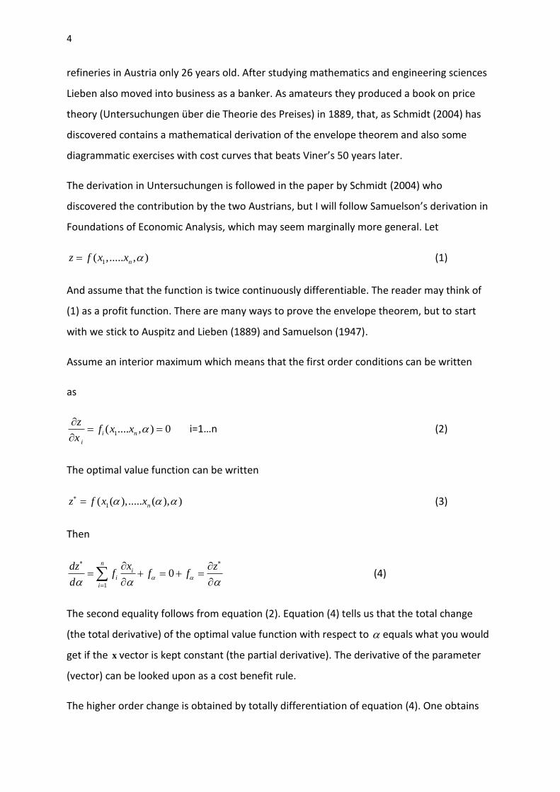
The derivation in Untersuchungen is followed in the paper by Schmidt (2004) who

discovered the contribution by the two Austrians, but I will follow Samuelson’s derivation in

Foundations of Economic Analysis, which may seem marginally more general. Let

1( ,..... , )nz f x x (1)

And assume that the function is twice continuously differentiable. The reader may think of

(1) as a profit function. There are many ways to prove the envelope theorem, but to start

with we stick to Auspitz and Lieben (1889) and Samuelson (1947).

Assume an interior maximum which means that the first order conditions can be written

as

1( .... , ) 0i n

i

zf x x

x

i=1…n (2)

The optimal value function can be written

1( ( ),..... ( ), )

nz f x x (3)

Then

1

0n

ii

i

xdz zf f f

d

(4)

The second equality follows from equation (2). Equation (4) tells us that the total change

(the total derivative) of the optimal value function with respect to equals what you would

get if the x vector is kept constant (the partial derivative). The derivative of the parameter

(vector) can be looked upon as a cost benefit rule.

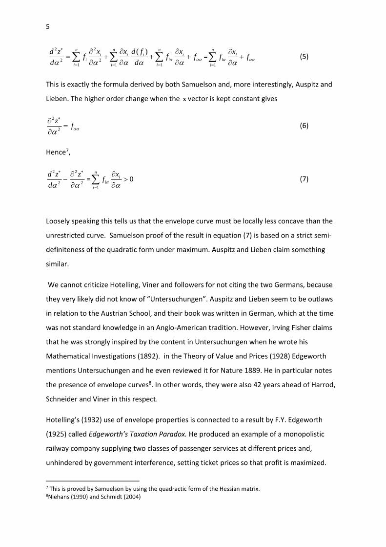
The higher order change is obtained by totally differentiation of equation (4). One obtains

5

22

2 21 1 1

( )n n ni i i i

i i

i i i

x x d f xd zf f f

d d

=

1

ni

i

i

xf f

(5)

This is exactly the formula derived by both Samuelson and, more interestingly, Auspitz and

Lieben. The higher order change when the x vector is kept constant gives

2

2

zf

(6)

Hence7,

2

2

d z

d

2

2

z

=

1

0n

ii

i

xf

(7)

Loosely speaking this tells us that the envelope curve must be locally less concave than the

unrestricted curve. Samuelson proof of the result in equation (7) is based on a strict semi-

definiteness of the quadratic form under maximum. Auspitz and Lieben claim something

similar.

We cannot criticize Hotelling, Viner and followers for not citing the two Germans, because

they very likely did not know of “Untersuchungen”. Auspitz and Lieben seem to be outlaws

in relation to the Austrian School, and their book was written in German, which at the time

was not standard knowledge in an Anglo-American tradition. However, Irving Fisher claims

that he was strongly inspired by the content in Untersuchungen when he wrote his

Mathematical Investigations (1892). in the Theory of Value and Prices (1928) Edgeworth

mentions Untersuchungen and he even reviewed it for Nature 1889. He in particular notes

the presence of envelope curves8. In other words, they were also 42 years ahead of Harrod,

Schneider and Viner in this respect.

Hotelling’s (1932) use of envelope properties is connected to a result by F.Y. Edgeworth

(1925) called Edgeworth’s Taxation Paradox. He produced an example of a monopolistic

railway company supplying two classes of passenger services at different prices and,

unhindered by government interference, setting ticket prices so that profit is maximized.

7 This is proved by Samuelson by using the quadractic form of the Hessian matrix. 8Niehans (1990) and Schmidt (2004)

6

When the railway company has to pay a tax on each first class ticket it may happen that both

the first and the second class tickets are decreased at profit maximum. Hotelling generalizes

this result by proving rigorously what mechanisms are involved, both under monopoly and

perfect competition. For the case of perfect competition he shows how a marginal change in

taxation results in a first and second order change, where the first order change disappears,

since demands equal supplies in general equilibrium. The second order change consists of

the so called Harberger triangles that were reinvented long after Hotelling’s cost-benefit

analysis of taxation.

Rene Roy’s identity was produced in Roy (1947) and the proof of the result is in line with

Auspitz and Lieben in that he uses the first order conditions of utility maximization. He also

cites Irving Fisher as an example of an author of early mathematical economics. Fisher was,

as mentioned above, inspired by Auspitz and Lieben, but he probably did not get stuck on

the envelope side of their book.

Ronald Shephard’s Lemma appears on page 13 in Shephard (1953) and follows from results

from convex theory and by an old theorem by Minkowski (1911), but it is also derived from a

distance function approach.

One cannot help to reflect over why so many economists, typically independent of each

other, have ended up proving the same result over and over again, and getting credit in

terms of their own name attached to the result. My reflections have so far not ended up in

any complete answer, but the following story by Erwin Diewert explains how Shephards

lemma surfaced9:

I was a Ph.D student at Berkeley, 1964-1968 (got my degree in 1969) so I did indeed

overlap with Shephard at that time but I did not take any courses from him. I did see

him occasionally in the Econometrics Workshop, which I attended for the 4 years I

was at Berkeley so I knew who he was.

I had a summer job in Ottawa in 1967 for the Department of Manpower and

Immigration, trying to predict the demand for different types of labour. I was not

happy with the Leontief type production functions that they were estimating at the

9 E.mail communication with Erwin Diewert.

7

time so I thought that I would generalize the functional form to allow for substitution.

The demand function I estimated had the following functional form for input 1 say:

(1) 1 1

1 11 12 2 1 1 1{ .... }

n nx a a p p a p p y

where

1x demand for input 1;

np = nth input price

y output

I presented my empirical results on Manpower demand in Canada using the above

functional form in the econometric workshop. Dan McFadden was in the audience

and said to me: “Erwin, your demand functions are not integrable!” I had no idea

what he was talking about but he told me to read his 1966 Berkeley working paper on

duality theory as well as Shephard’s 1953 book, which I did. And I realized that if I

simply took the square roots of the input price ratios on the right hand side of the

demand equations of the form (1), then my demand functions would be integrable

(with symmetric conditions imposed) and thus was born the Generalized Leontief

production and cost functions. In my reading of Shephard’s 1953 book, I realized that

he provided a proof of “Shephard’s Lemma” starting from the cost function (as

opposed to Hicks in Value and Capital, who started with the production or utility

function and derived the result). So I named Shephard’s result “Shephard’s Lemma”

in my first Berkeley discussion paper on the Generalized Leontief Production

Function (later published in the Journal of Political Economy in 1971) and in my 1969

thesis. So I was certainly influenced by Shephard but at that stage, it was only by

reading his book. I went on and did my thesis on flexible functional forms under the

direction of McFadden.

Later on during the 1970s and 1980s, our paths crossed at the Index number

workshops that Wolfgang Eichhorn held in Karlsruhe. At first Shephard did not much

like me (he thought that I was stealing his stuff) but later on, he realized that my

papers were making him more famous than ever and we got along quite well.

So that is my story on the origins of the term “Shephard’s Lemma”.

8

4. Calculus of Variations and Envelope Theorems

The calculus of variations was initiated by Galileo Galilei (1564-1642) and Johann Bernoulli

(1667-1748). Galilei was thinking about the brachistochrone problem, “the slide of quickest

decent without friction”. He did not solve it himself. It was Johann Bernoulli that settled the

problem in 1696. He showed that the optimal curve is a cycloid; a circle shaped curve that is

mapped from a fixed point on the periphery of a circle when the circle rotates. A quarter of a

century later Bernouili proposed to his student Leonard Euler to take up the task of finding

general methods to solve similar problems. This started the calculus of variations. In 1759

Euler received a letter from the young Joseph Lagrange that contained a proof of necessary

conditions which also involved the germ of the multiplier rule for a calculus of variations

problem with constraints. Euler wrote back and told Lagrange that he also had done

progress but would refrain from publishing his results until Lagrange had published his. That

is scientific generosity!

To be honest I have not even skimmed the literature on the calculus of variations after Euler,

but I doubt there is any envelope result until the dissertation by Ernst Zermerlo in 1894.It is,

however , not easy to understand. I have tried to read Zermerlo’s thesis, and it was by no

means easy. However, as far as I can understand, he was up to finding necessary conditions

for an optimal path. The envelope theorem comes as the closing key result of the thesis. The

problem looks very much the same as what a general calculus of variations problem looks

like today. He starts from Weierstrass10 who was standing on the axis of Euler and Lagrange.

The diagram below is an illustration of the theorem.

10 Karl Weierstrass (1815-1897) German mathematician who did important contribution to real analysis and the calculus of variations. He introduced uniform convergence into mathematics. He also showed that there exists a closed graph that has no tangent at any point. A Brownian motion process is one example. I am not sure that Bachelier (1900) and Einstein (1905) discovered that.

9

Figure 1: Illustration of Zermerlo’s envelope theorem.

The bold curve is an envelope to the optimal solution curve a and u is a curve that starts at

zero on the optimal curve and joins the envelope in point 4. The optimal curve starts at 1

and ends at 2, and at 3 it is a tangent to the envelope. The optimal value function is given by

12J 2

1

( ( ), ( ), ; )

t

t

F y t y t t k dt

. Zermerlo proves that the variation 043 from 03 vanishes when

the Value functions are integrated in the following manner

3

4

043 03( ) 0J J E d

This means that

10432 12J J

The disturbed part of the optimal path does not matter. The details are available in

Zermerlo11 (1894), but I do not recommend economists to spend too much time on them.

11 Zermerlo was not the only one that produced envelope theorems in the calculus of variations. Darboux (1894) and Knerser (1898) were two others. Zermerlo is today quite well known among game theorists. He was the first to discuss whether chess has a solution in Zermerlo (1913). His theorem says that either white or black has a winning strategy or both can force a draw. The proof had some blemishes, pointed out by König (1927) and the proof was rectified by both of them. There are two paragraphs in König (1927) where Zermerlo’s way to fix his proof is shown. See Larson (2008).

0

1

4

3

2

Envelope

u

a

10

My guess is that the theorem is related to the same class of results as the Fundamental

Theorem of the Calculus of Variations12. It is, however, not clear to me how Zermerlo’s

theorem can help to find the optimal path. He comments his accomplishment in the

following manner (author’s translation from German).

“This result is essentially a generalization of a property of a catenary first discovered by mr

Lindelöf (Moigno and Lindelöf, Lecons di Calcul Differential e Integral IV Calcul de Variations)

covering the contents of surfaces of revolution yds by which two surfaces have separated

tangents in terms of envelopes . On the other hand, it lacks me so far a simple criterion for

the existence of a general envelope from the assumed properties.”

The function ( )E is a construction of Weierstrass that is non negative but zero in this

particular situation. A catenary is the curve that an idealized hanging chain or cable assumes

when supported at its ends and acted only by its weight. A surface of revolution is a surface

in Euclidian space created by rotating a curve around a straight line.

4. Optimal Control Theory

The envelope theorems in optimal control theory are in principle of the same character as

the static ones. The “classical result” must, in a sense, have been known already by William

Rowan Hamilton, who13 in 1833 reformulated classical mechanics into Hamilton dynamics.

He built on a previous reformulation of Joseph Lagrange from 1788. The Hamilton equations

provide a new and equivalent method of looking at classical mechanics. They are not simpler

to solve but provide new insights. I do not know physics, so I will give the economic

interpretation of the Hamilton equations by starting from a Ramsey problem14. Ramsey’s

version was an optimal intertemporal saving problem that he solved in spite of the fact that

the value function was unbounded15. The following optimization problem is, except for the

upper integration level of the value function, a version of Ramsey’s original problem.

12 See e.g. Seierstad and Sydsaeter (1987) chapter 1. 13 He is also well known for his four dimensional complex number theory (quarternions) and his drinking habits. He died from gaut 63 years old. 14 Developed by Frank Plumpton Ramsey (1928) 15 The reason was that he did not like discounting due to ethical reasons.

11

0( )

0

( ), ( ), ; )

T

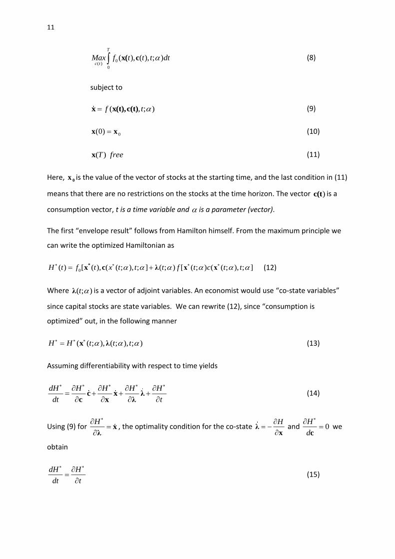
c tMax f t t t dt x( c (8)

subject to

( , ; )f t x x(t),c(t) (9)

0)0( xx (10)

freeT)(x (11)

Here, 0x is the value of the vector of stocks at the starting time, and the last condition in (11)

means that there are no restrictions on the stocks at the time horizon. The vector )c(t is a

consumption vector, t is a time variable and is a parameter (vector).

The first “envelope result” follows from Hamilton himself. From the maximum principle we

can write the optimized Hamiltonian as

0( ) [ ( ), ( ( ; ), ; ] ( ; ) [ ( ; ) ( ( ; ), ; ]H t f t x t t t f t c t t

*

x c λ x x (12)

Where ( ; )t λ is a vector of adjoint variables. An economist would use “co-state variables”

since capital stocks are state variables. We can rewrite (12), since “consumption is

optimized” out, in the following manner

( ( ; ), ( ; ), ; )H H t t t x λ (13)

Assuming differentiability with respect to time yields

dH H H H H

dt t

c x λc x λ

(14)

Using (9) for H

xλ

, the optimality condition for the co-state H

λx

and 0H

d

c

we

obtain

dH H

dt t

(15)

12

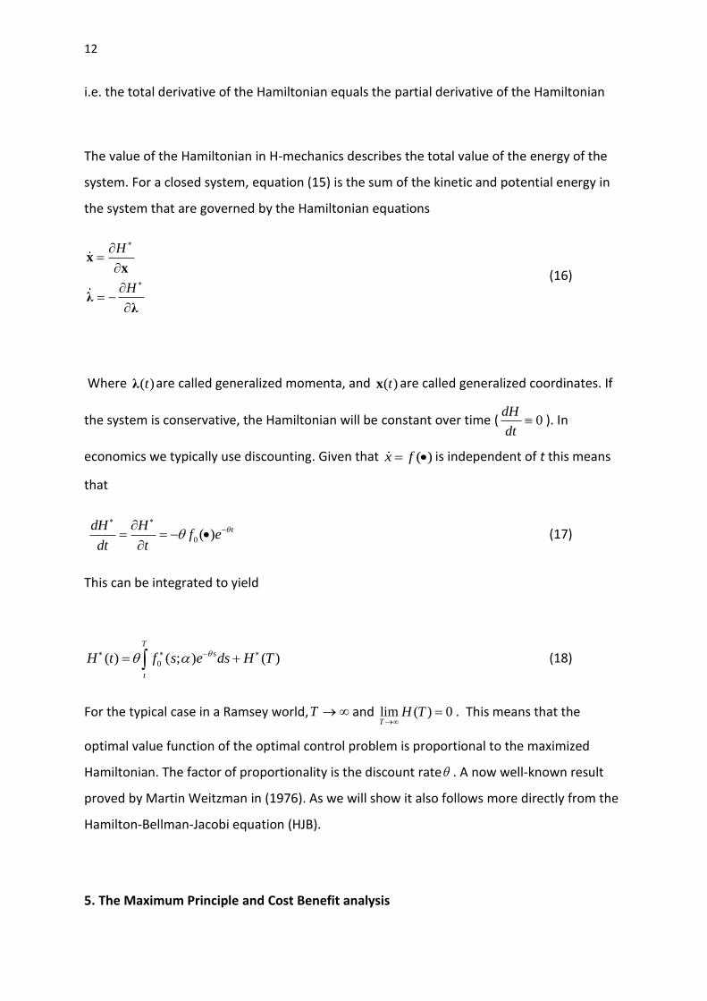
i.e. the total derivative of the Hamiltonian equals the partial derivative of the Hamiltonian

The value of the Hamiltonian in H-mechanics describes the total value of the energy of the

system. For a closed system, equation (15) is the sum of the kinetic and potential energy in

the system that are governed by the Hamiltonian equations

H

H

xx

λλ

(16)

Where ( )tλ are called generalized momenta, and ( )tx are called generalized coordinates. If

the system is conservative, the Hamiltonian will be constant over time ( 0dH

dt ). In

economics we typically use discounting. Given that ( )x f is independent of t this means

that

0( )

tdH Hf e

dt t

(17)

This can be integrated to yield

0( ) ( ; ) ( )

T

s

t

H t f s e ds H T

(18)

For the typical case in a Ramsey world,T and lim ( ) 0T

H T

. This means that the

optimal value function of the optimal control problem is proportional to the maximized

Hamiltonian. The factor of proportionality is the discount rate . A now well-known result

proved by Martin Weitzman in (1976). As we will show it also follows more directly from the

Hamilton-Bellman-Jacobi equation (HJB).

5. The Maximum Principle and Cost Benefit analysis

13

Cost Benefit analysis is certainly an economic technique that has been improved by envelope

results. The first time this was done is probably Hotelling’s discussion of Edgeworth’s

taxation paradox, where he uses that excess demand in general equilibrium is zero implying

that all the terms of first degree vanishes in the tax rates, to come up with his result.

Here we will show how cost benefit analysis is done in a dynamic context using envelope

properties.

Let us start by rewriting the optimal value function above in the following manner16

0

( , , ; )

{ [ ( , ), ( , ), ; ] ( , ) [ ( , ), ( , ); ] ( , )}

[ ( , ), ( , ), ( , ), ; ] ( ) ( ) ( ) ( ) ( ) ( )

t

T

s

t

T T

t t

V t T

f x s s s e s f s s s ds

H s s s s ds t t T T s s ds

x

c λ x c x

x c λ λ x λ x λ x

(19)

To obtain the third line partial integration has been used. We can now differentiate the

value function with respect to the lower integration level, the upper integration level and

the capital stock at time t, ( )

tt x x .

We start with the derivative of the lower integration level to get

( ) ( ) ( ) ( ) ( ) ( ) ( )V

H t t t t t t tt

λ x λ x λ x = ( )H t (20)

Since, ( )t

t x x is a constant ( ) 0t x . For similar reasons ( )V

H TT

. Finally it follows

Immediately from equation (19) that ( )t

Vt

λ

x. The latter vector (the adjoint vector) tells us

about the value of an extra unit of capital at time t (the shadow prices of the capital stocks

or state variables.

16 This trick is due to an idea by Leonard (1987). He is also worth an envelope theorem.

14

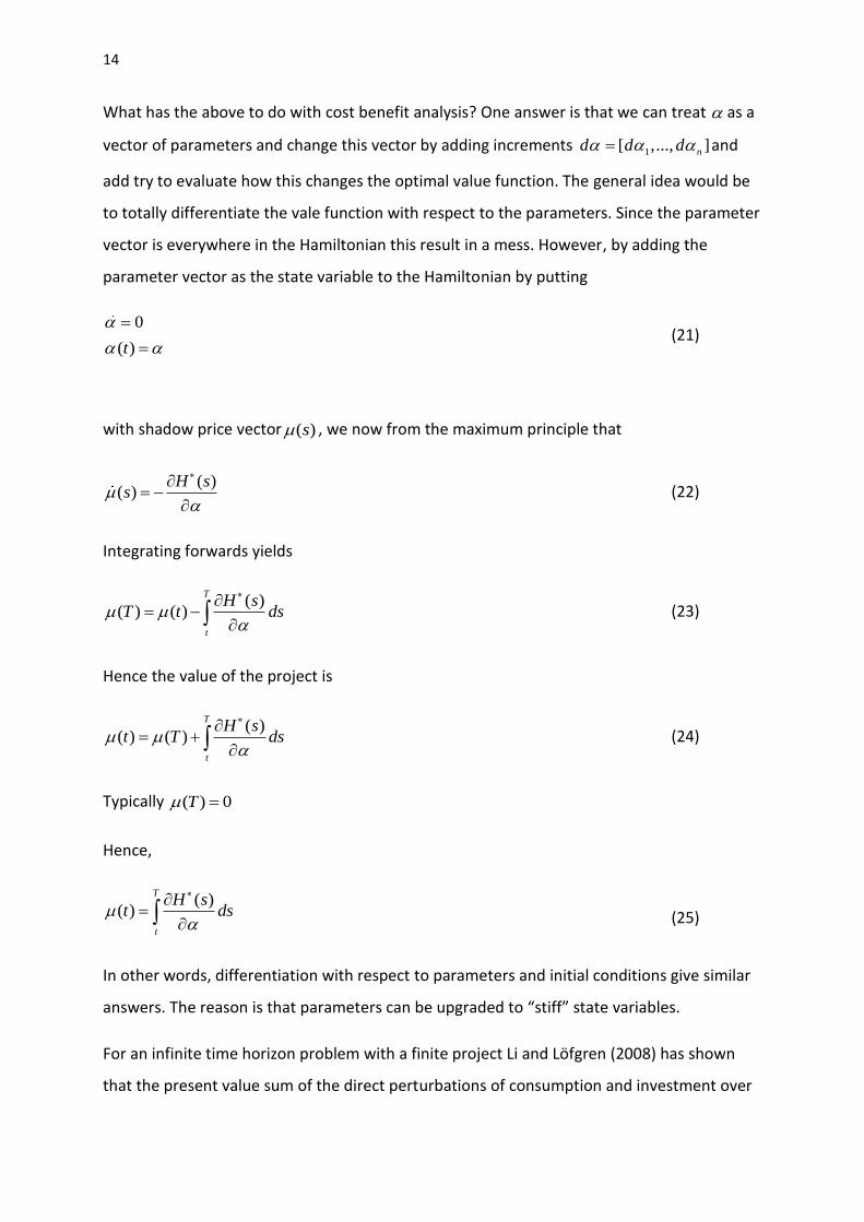
What has the above to do with cost benefit analysis? One answer is that we can treat as a

vector of parameters and change this vector by adding increments 1[ ,..., ]nd d d and

add try to evaluate how this changes the optimal value function. The general idea would be

to totally differentiate the vale function with respect to the parameters. Since the parameter

vector is everywhere in the Hamiltonian this result in a mess. However, by adding the

parameter vector as the state variable to the Hamiltonian by putting

0

( )t

(21)

with shadow price vector ( )s , we now from the maximum principle that

( )( )

H ss

(22)

Integrating forwards yields

( )( ) ( )

T

t

H sT t ds

(23)

Hence the value of the project is

( )( ) ( )

T

t

H st T ds

(24)

Typically ( ) 0T

Hence,

( )( )

T

t

H st ds

(25)

In other words, differentiation with respect to parameters and initial conditions give similar

answers. The reason is that parameters can be upgraded to “stiff” state variables.

For an infinite time horizon problem with a finite project Li and Löfgren (2008) has shown

that the present value sum of the direct perturbations of consumption and investment over

15

the finite project period will give us the value of the project. Note that the cost-benefit rule

both in equation (24) and the result in Li and Löfgren (2008) does not involve indirect

general equilibrium effects. The reason is that we obtain envelope properties along the

optimal path17. Li and Löfgren in addition show that the direct net effect during the project

period is enough to obtain a correct answer. To see this we start from a rather straight

forward cost-benefit rule and a related cost-benefit rule by Dixit et al. 1980.

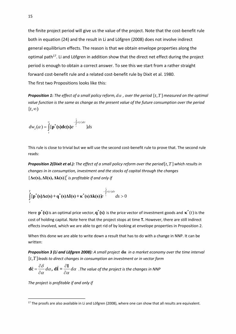
The first two Propositions looks like this:

Proposition 1: The effect of a small policy reform, d , over the period [ , ]t T measured on the optimal

value function is the same as change as the present value of the future consumption over the period

[ , )t

This rule is close to trivial but we will use the second cost-benefit rule to prove that. The second rule

reads:

Proposition 2(Dixit et al.): The effect of a small policy reform over the period[ , ]t T which results in

changes in in consumption, investment and the stocks of capital through the changes

[ ]T

tΔc(s), ΔI(s), Δk(s) is profitable if and only if

( )

[ ] 0

s

t

T r d

t

e ds

* * *

p (s)Δc(s) + q (s)ΔI(s) + κ (s)Δk(s)

Here *p (s) is an optimal price vector, *

q (s) is the price vector of investment goods and ( )t*

κ is the

cost of holding capital. Note here that the project stops at time T. However, there are still indirect

effects involved, which we are able to get rid of by looking at envelope properties in Proposition 2.

When this done we are able to write down a result that has to do with a change in NNP. It can be

written:

Proposition 3 (Li and Löfgren 2008): A small project dα in a market economy over the time interval

[ , ]t T leads to direct changes in consumption an investment or in vector form

d d

Idc , dI = .The value of the project is the changes in NNP

The project is profitable if and only if

17 The proofs are also available in Li and Löfgren (2008), where one can show that all results are equivalent.

( )

2( ) [ ]

s

t

r d

t

dw e ds

*

p (s)dc(s)

16

( )

[ ( ) (s) ( ) dI(s]e

T

t

T r d

t

s c s ds

*

p d q >0

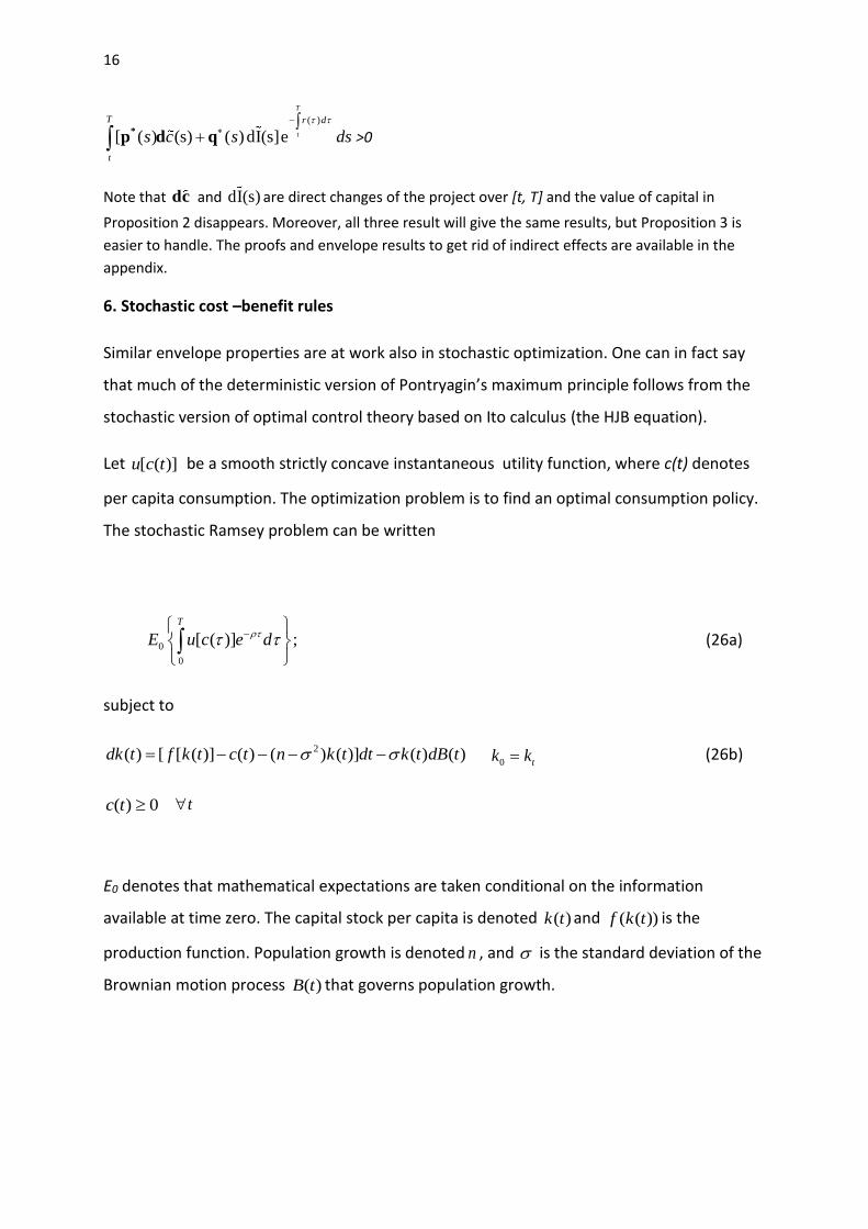
Note that dc and dI(s) are direct changes of the project over [t, T] and the value of capital in

Proposition 2 disappears. Moreover, all three result will give the same results, but Proposition 3 is

easier to handle. The proofs and envelope results to get rid of indirect effects are available in the

appendix.

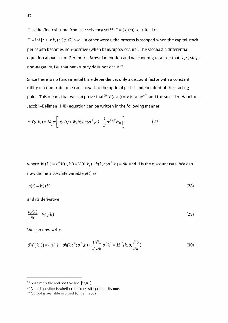
6. Stochastic cost –benefit rules

Similar envelope properties are at work also in stochastic optimization. One can in fact say

that much of the deterministic version of Pontryagin’s maximum principle follows from the

stochastic version of optimal control theory based on Ito calculus (the HJB equation).

Let [ ( )]u c t be a smooth strictly concave instantaneous utility function, where c(t) denotes

per capita consumption. The optimization problem is to find an optimal consumption policy.

The stochastic Ramsey problem can be written

0

0

[ ( )] ;

T

E u c e d

(26a)

subject to

2( ) [ [ ( )] ( ) ( ) ( )] ( ) ( )dk t f k t c t n k t dt k t dB t

0 tk k (26b)

0)( tc t

E0 denotes that mathematical expectations are taken conditional on the information

available at time zero. The capital stock per capita is denoted ( )k t and ( ( ))f k t is the

production function. Population growth is denoted n , and is the standard deviation of the

Brownian motion process ( )B t that governs population growth.

17

T is the first exit time from the solvency set18 { ( ); 0}G k k , i.e.

inf{ ; ( ) }T s k G . In other words, the process is stopped when the capital stock

per capita becomes non-positive (when bankruptcy occurs). The stochastic differential

equation above is not Geometric Brownian motion and we cannot guarantee that ( )k stays

non-negative, i.e. that bankruptcy does not occur19.

Since there is no fundamental time dependence, only a discount factor with a constant

utility discount rate, one can show that the optimal path is independent of the starting

point. This means that we can prove that20 t

tt ekVktV

),0(),( and the so called Hamilton-

Jacobi –Bellman (HJB) equation can be written in the following manner

2)

2 2

t k kkc

1W(t,k Max u(c(t) W h(k,c; ,n) k W

2

(27)

where ( ) ( , ) (0, )t

t t tW k e V t k V k

, 2

( , ; , )h k c n dk and is the discount rate. We can

now define a co-state variable p(t) as

( ) ( )kp t W k (28)

and its derivative

( )( )

kk

p tW k

t

(29)

We can now write

2 c* * 2 2

t

1 p pW k ) u(c ) ph(k,c ; ,n) k H (k, p, )

2 k k

(30)

18 G is simply the real positive line [0, ) 19 A hard question is whether it occurs with probability one. 20 A proof is available in Li and Löfgren (2009).

18

The function )(

cH can be interpreted as a “generalized” optimized Hamiltonian in current

value terms. Similar to Weitzman theorem ( H V ), the HJB equation shows that the

generalized current value Hamiltonian is directly proportional to the optimal value function.

Moreover, and also interesting, is that by putting 0 equation (30) collapses to

Weitzman’s theorem. In fact, also the co-state and state equations collapses to those of the

maximum principle21. One can say that most of the maximum principle follows as a special

case from stochastic optimal control.

Moreover, the cost benefit rule that was derived above looks the same, when you take

expectations of the stochastic co-state equation that represents the cost benefit project.

More precisely, it can be written:

( )( ) { }

t

Hp t E

d

(31)

Again envelope properties are involved. The reader is referred to a memoranda by Aronsson,

Löfgren and Nyström (2003) and Aronsson Löfgren and Backlund (2004) for technicalities.

Chapter 9 in the latter reference and Malliaris and Brock (1982) tell us more in detail how

the HJB-equation and the maximum principle fit together.

Conclusions

It is not easy to sum up the contents of the paper. My curiosity may have put me astray, and

the paper reminds me of a small smörgåsbord, which at least contains herring, salmon, fish

eggs, sausages, meatballs , ham, pate’ and almond potatoes. It is obvious that it does not

contain the comprehensive story of envelope theorems, but I have hopefully conveyed the

message on the importance of them for economic analysis. Optimization helps to produce

them. Another message is that they are easy to handle. As Eugene Silberberg (1974, 1978)

very wittedly has pointed out, the calculations can be carried out at the “back of an

envelope”. Finally, they are old and have been discovered by many.

21 See Malliaris and Brock (1982)

19

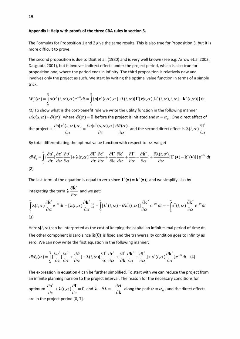
Appendix I: Help with proofs of the three CBA rules in section 5.

The Formulas for Proposition 1 and 2 give the same results. This is also true for Proposition 3, but it is

more difficult to prove.

The second proposition is due to Dixit et al. (1980) and is very well known (see e.g. Arrow et.al.2003;

Dasgupta 2001), but it involves indirect effects under the project period, which is also true for

proposition one, where the period ends in infinity. The third proposition is relatively new and

involves only the project as such. We start by writing the optimal value function in terms of a simple

trick.

0

0

( ) ( ( , ), ) { [ ( . ), ] ( , )[ [ , ), ( , ), , ] ( )]}dtt

o

W u t e dt u t t (t t t t,

c c λ I c k k

(1) To show what is the cost-benefit rule we write the utility function in the following manner

[ ( , ) ( )]u c s where ( ) 0 before the project is initiated and 0 . One direct effect of

the project is [ ( , ), ] [ ( , ), ] ( )u s u s

c

c c and the second direct effect is ( , )t

Iλ

By total differentiating the optimal value function with respect to we get

0

0

( , ){ [ ] ( , )[ ] [ ( ) ( )]}e

tu tdW t dt

c I c I k I k λλ I k

c c k

(2)

The last term of the equation is equal to zero since ( ) ( )] I k and we simplify also by

integrating the term

kλ and we get:

0

0 0 0

( , ) [ ( , ) ] [ ( , ) ( , )] e ( , )t t t

t e dt t t t dt t e dt

*k k k kλ λ λ λ s

(3)

Here , )t s( can be interpreted as the cost of keeping the capital an infinitesimal period of time dt.

The other component is zero since (0)k is fixed and the tranversality condition goes to infinity as

zero. We can now write the first equation in the following manner:

0

0

( ) { [ ] ( , )[ ] ( , ) }tu

dW t t e dt

c I c I k I kλ s

c c k (4)

The expression in equation 4 can be further simplified. To start with we can reduce the project from

an infinite planning horzion to the project interval. The reason for the necessary conditions for

optimum ( , ) 0u

tc c

Iλ and

H

λ λ

k along the path 0

, and the direct effects

are in the project period [0, T].

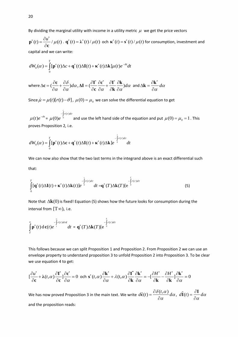
20

By dividing the marginal utility with income in a utility metric we get the price vectors

( ) / ( )u

t t

pc

. ( ) ( ) / ( )t t t q λ och ( ) ( ) / ( )t t t

κ s for consumption, investment and

capital and we can write:

0

0

( ) [ ( ) ( ) ( ) ( ) ] ( )

T

tdW t c t t t t e dt

p q I κ k

where ( ) , ( )d d

c I c I kc ΔI

c k and d

kk

Since ( )[ ( ) ]t r t , 0(0) we can solve the differential equation to get

( )t

t e = 0

( )

(0)

t

r d

e

and use the left hand side of the equation and put 0(0) 1 . This

proves Proposition 2, i.e.

0

( )

0

0

( ) [ ( ) ( ) ( ) ( ) ]

t

T r d

dW t t t t e dt

p c q I κ k

We can now also show that the two last terms in the integrand above is an exact differential such

that:

0 0

( ) ( )

0

[ ( ) ( ) ( ) ( )] ( ) ( )[e

t T

T r d r d

t t t t e dt T T

q I κ k q k (5)

Note that (0)k is fixed! Equation (5) shows how the future looks for consumption during the

interval from [T ), i.e.

( )

( ) d ( ) t

r d d

T

t t e dt

p c = 0

( )

( ) ( )[e

T

r d

T T

q k

This follows because we can split Proposition 1 and Proposition 2. From Proposition 2 we can use an

envelope property to understand proposition 3 to unfold Proposition 2 into Proposition 3. To be clear

we use equation 4 to get:

[ ( , ) ] 0u

t

I cλ

c c och ( , ) (t, ) [ ] 0

H Ht

*k I k k

sk k k

We has now proved Proposition 3 in the main text. We write ( , )

( ) ,t

d t d

c ( )d t d

II

and the proposition reads:

21

( )

[ ( ) (s) ( ) dI(s]e

T

t

T r d

t

s c s ds

*

p d q

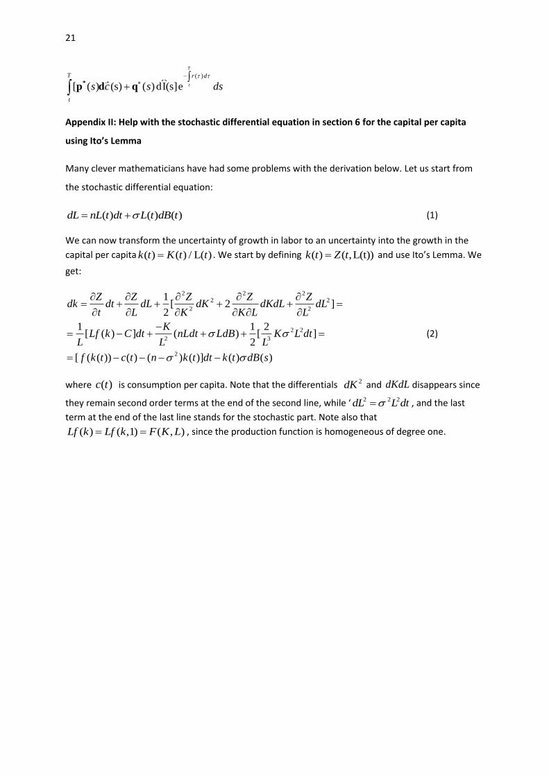
Appendix II: Help with the stochastic differential equation in section 6 for the capital per capita

using Ito’s Lemma

Many clever mathematicians have had some problems with the derivation below. Let us start from

the stochastic differential equation:

( ) ( ) ( )dL nL t dt L t dB t (1)

We can now transform the uncertainty of growth in labor to an uncertainty into the growth in the

capital per capita ( ) ( ) / L( )k t K t t . We start by defining ( ) ( ,L(t))k t Z t and use Ito’s Lemma. We

get:

2 2 22 2

2 2

2 2

2 3

2

1[ 2 ]

2

1 1 2[ ( ) ] ( ) [ ]

2

[ ( ( )) ( ) ( ) ( )] ( ) ( )

Z Z Z Z Zdk dt dL dK dKdL dL

t L K K L L

KLf k C dt nLdt LdB K L dt

L L L

f k t c t n k t dt k t dB s

(2)

where ( )c t is consumption per capita. Note that the differentials 2dK and dKdL disappears since

they remain second order terms at the end of the second line, while ‘ 2 2 2dL L dt , and the last

term at the end of the last line stands for the stochastic part. Note also that

( ) ( ,1) ( , )Lf k Lf k F K L , since the production function is homogeneous of degree one.

22

References

Aronsson, T., Löfgren K.G., and Backlund, K. (2004) Welfare Measurement in Imperfect

Markets: A growth Theoretical Approach. Cheltenham: Edward Elgar.

Aronsson, T. Löfgren K.G. and Nyström, K. (2003) Stochastic Cost Benefit Rules: A Back of the

Lottery Ticket Calculation Method, Umeå Economic Studies, No 606.

Arrow, K., Dasgupta, P. and Mäler, K.G. (20039 Evaluating Projects and Assessing Sustainable

Development in Imperfect Market, Environment and Resource Economics 26, 647-685.

Arrow, K., and Kurz, M. (1970) Public Investment and The Rate of Return, Washington DC:RFF

Auspitz,R. and Lieben R. (1889) Untersuchungen über die Theorie des Preises. Leipzig: Verlag

von Duncker & Humblot.

Bachlier, L (1900) Theorie de la Speculation, Annales l’Ecole Normale Superieure 17 , 21-86.

Benveniste, L.M. and Scheinkman, J.A.On the Differentiability of the Value Function in

Dynamic Models of Economics, Econometrica 47, 727-32.

Caputo, M.R.(1990a)Comparative Dynamics with Envelope Methods in Variational Calculus,

Review of Economic Studies 57, 689-97.

Caputo, M.R. (1990b)How to do Comparative Dynamics on the Back of an Envelope in

Optimal Control Theory, Journal of Economic Dynamics and Control, 14, 655-83.

Courant, R and John, F (1974) Introduction to Calculus and Analysis (volume2) New York:

John Wiley and Sons.

Darboux, J.G. (1894) Lecons sur la Theorie Generale des Surfaces, Band 2, Buch 5.

Dixit, A., Hammond, P. and Hoel,M (1980) On Hartwick’ s Rule for Regular Maximins Path of

Capital Accumulation and Resource Depletion, Review of Economic Studies 47, 551-556.

Edgeworth,F.Y.(1889)The Mathematical Method in Political Economy. (Review of

Untersuchungen über dieTheorie des Preises.) Nature 40, 242-44.

23

Einstein, A. (1956) Investigation on the Theory of Brownian Motion, New York: Dover

(contains his seminal paper from 1905)

Fisher, I. [(1882), 1925] Mathematical Investigations in the Theory of Value and Prices, New

Haven: Yale University Press (reprint of Fisher’s dissertation).

Harrod, R.F. (1931) The Law of Decreasing Costs, Economic Journal 41, 566-76.

Hotelling, H. (1932) Edgeworth Taxation Paradox and the Nature of Demand and Supply

Functions, Journal of Political Economy 39, 577-616.

Kneser, A. (1898) Ableitung hinreichender Bedingungen des Maximum oder Minimum

einfacher Integrale aus der Theorie der Zweiten Variation. Math.Annalen, Band 51.

König, D. Über eine Schlussweisse aus dem Endlichen ins Uendliche, Acta Sci. Math. Szeged #

(1927), 121-130.

La France, J.T. and Barney, L.D. (1991) The Envelope Theorem in Dynamic Optimization,

Journal of Dynamic and Control 15, 355-85.

Larson, P.B. (2008) Introduction to Zermelo’s 1913 and 1927b, mimeo Department of

Mathematics and Statistics, Miami University, Oxford Ohio.

Leonard, D. (1987) Co-state Variables Correctly Value Stocks at Each Instant of Time, Journal

of Economic Dynamics and Control 11, 117-22.

Li, C.Z. and Löfgren, K.G. (2008) Evaluating Project in a Dynamic Economy: Some New

Envelope Results, German Economic Review 9, 1-16.

Li, C.Z. and Löfgren, K.G.(2012) Genuine Saving under Stochastic Growth, Letters in Spatial

Science and Resources 5, 167-174.

Malanowski, K. (1984) On Differentiability with Respect to Parameter of Solutions to Convex

Optimal Control Problems Subject to State Space Constraints, Applied Mathematics and

Optimization 12, 231-45.

Malliaris A.G. and Brock W.A.(1991) Stochastic Methods in Economics and Finance,

Amsterdam: North Holland.

24

Niehans, J. (1990) A History of Economic Theory: Classic Contributions 1720-1980, Baltimore:

Johns Hopkins.

Oniki, H.(1971) Comparative Dynamics (Sensivity Analysis) in Optimal Control Theory, Journal

of Economic Theory 6, 265-83.

Ramsey, F.P.(1928) A Mathematical Theory of Saving, Economic Journal 38, 543-59.

Roy. R (1947) La Distribution Du Revenu Entre Les Divers Biens, Econometrica 15, 205-25.

Rudin, W (1976) Principles of Mathematical Analysis, Tokyo: McGraw- Hill.

Samuelson, P.A. (1947) Foundations of Economic Analysis, Cambridge: Harvard University

Press.

Schmidt, T. (2004) Really Pushing the Envelope: Early Use of the Envelope Theorem by

Auspitz and Lieben, History of Political Economy 36, 103-129.

Schneider, E. (1931) Kostentheoretisches zum Monopolproblem, Zeischrift für

Nationalökonomie 3.2, 185-211.

Seierstad, A. (1981) Derivatives and Subderivatives of the Optimal Value Function in Control

Theory, Institute of Economics memorandum Feb 26, University of Oslo.

Seierstad, A. (1982) Differentiability Properties of the Optimal Value Function in Control

Theory, Journal of Economic Dynamics and Control 4,303-10.

Seierstad, A.and Sydsaeter, K. (1987) Optimal Control Theory with Economic Applications,

Amsterdam: Norh Holland.

Shephard, R. (1953) Cost and Production Functions, Princeton: Princeton University Press.

Silberberg, E (1974) A Revision of the Comparative Static Terminology in Economics, or, How

to do Comparative Statics on the Back of an Envelope, Journal of Economic Theory 7, 169-72.

Siberberg, E. (1978) The Structure of Economics: A Mathematical Analysis, New York:

McGraw Hill

Viner, J (1931) Cost Curves and Supply Curves, Zeischrift für Nationalökonomie 3.1, 26-46.

25

Widder, D. V. (1961) Advanced Calculus, Englewood Cliffs: Prentice Hall.

Zermelo, E (1894) Untersuchungen zur Variations-Rechnung, Berlin (dissertation)

Zermerlo, E. (1913) Über eine Anwendung der Megenlehre auf die Theorie des Schachspiels,

Proc, Fifth Congress Mathematicians, (Cambridge 1912), Cambridge University Press 1913,

501-504.