A BRIEF LIST OF MATLAB COMMANDS

Some Basic Commands (Note command syntax is case-sensitive!)

matlab loads the program matlab into your workspace.

quit quits matlab, returning you to the operating system.

exit same as quit.

who lists all of the variables in your matlab workspace.

whos list the variables and describes their matrix size.

clear deletes all matrices from active workspace.

clear x deletes the matrix x from active workspace.

... the ellipsis defining a line continuation is three

successive periods.

save saves all the matrices defined in the current

session into the file, matlab.mat.

load loads contents of matlab.mat into current workspace.

save filename saves the contents of workspace into

filename.mat

save filename x y z

saves the matrices x, y and z into the file titled

filename.mat.

load filename loads the contents of filename into current

workspace; the file can be a binary (.mat) file

or an ASCII file.

! the ! preceding any unix command causes the unix

command to be executed from matlab.

Commands Useful in Plotting.

plot(x,y) creates an Cartesian plot of the vectors x & y.

plot(y) creates a plot of y vs. the numerical values of the

elements in the y-vector.

semilogx(x,y) plots log(x) vs y.

semilogy(x,y) plots x vs log(y)

loglog(x,y) plots log(x) vs log(y).

grid creates a grid on the graphics plot.

title('text') places a title at top of graphics plot.

xlabel('text') writes 'text' beneath the x-axis of a plot.

ylabel('text') writes 'text' beside the y-axis of a plot.

text(x,y,'text') writes 'text' at the location (x,y) .

text(x,y,'text','sc') writes 'text' at point x,y assuming

lower left corner is (0,0) and upper

right corner is (1,1).

gtext('text') writes text according to placement of mouse

hold on maintains the current plot in the graphics window

while executing subsequent plotting commands.

hold off turns OFF the 'hold on' option.

polar(theta,r) creates a polar plot of the vectors r & theta

where theta is in radians.

bar(x) creates a bar graph of the vector x. (Note also

the command stairs(y).)

bar(x,y) creates a bar-graph of the elements of the vector y,

locating the bars according to the vector elements

of 'x'. (Note also the command stairs(x,y).)

hist(x) creates a histogram. This differs from the bargraph

in that frequency is plotted on the vertical axis.

mesh(z) creates a surface in xyz space where z is a matrix

of the values of the function z(x,y). z can be

interpreted to be the height of the surface above

some xy reference plane.

surf(z) similar to mesh(z), only surface elements depict

the surface rather than a mesh grid.

contour(z) draws a contour map in xy space of the function

or surface z.

meshc(z) draws the surface z with a contour plot beneath it.

meshgrid [X,Y]=meshgrid(x,y) transforms the domain specified

by vectors x and y into arrays X and Y that can be

used in evaluating functions for 3D mesh/surf plots.

print sends the contents of graphics window to printer.

print filename -dps writes the contents of current

graphics to 'filename' in postscript format.

Equation Fitting

polyfit(x,y,n) returns the coefficients of the n-degree

polynomial for the vectors x and y. n must be at least 1

larger than the length of the vectors x and y. If n+1 =

length(x) the result is an interpolating polynomial. If

n+1 > length(x) the result is a least-squares polynomial

fit. The coefficients are stored in order with that of

the highest order term first and the lowest order last.

polyval(c,x) calculates the values of the polynomial whose

coefficients are stored in c, calculating for every

value of the vector x.

Data Analysis Commands

max(x) returns the maximum value of the elements in a

vector or if x is a matrix, returns a row vector

whose elements are the maximum values from each

respective column of the matrix.

min (x) returns the minimum of x (see max(x) for details).

mean(x) returns the mean value of the elements of a vector

or if x is a matrix, returns a row vector whose

elements are the mean value of the elements from

each column of the matrix.

median(x) same as mean(x), only returns the median value.

sum(x) returns the sum of the elements of a vector or if x

is a matrix, returns the sum of the elements from

each respective column of the matrix.

prod(x) same as sum(x), only returns the product of

elements.

std(x) returns the standard deviation of the elements of a

vector or if x is a matrix, a row vector whose

elements are the standard deviations of each

column of the matrix.

sort(x) sorts the values in the vector x or the columns of

a matrix and places them in ascending order. Note

that this command will destroy any association that

may exist between the elements in a row of matrix x.

hist(x) plots a histogram of the elements of vector, x. Ten

bins are scaled based on the max and min values.

hist(x,n) plots a histogram with 'n' bins scaled between the

max and min values of the elements.

hist((x(:,2)) plots a histogram of the elements of the 2nd

column from the matrix x.

fliplr(x) reverses the order of a vector. If x is a matrix,

this reverse the order of the columns in the matrix.

flipud(x) reverses the order of a matrix in the sense of

exchanging or reversing the order of the matrix

rows. This will not reverse a row vector!

reshape(A,m,n) reshapes the matrix A into an mxn matrix

from element (1,1) working column-wise.

SPECIAL MATRICES

zeros(n) creates an nxn matrix whose elements are zero.

zeros(m,n) creates a m-row, n-column matrix of zeros.

ones(n) creates a n x n square matrix whose elements are 1's

ones(m,n)' creates a mxn matrix whose elements are 1's.

ones(A) creates an m x n matrix of 1's, where m and n are

based on the size of an existing matrix, A.

zeros(A) creates an mxn matrix of 0's, where m and n are

based on the size of the existing matrix, A.

eye(n) creates the nxn identity matrix with 1's on the

diagonal.

Miscellaneous Commands

length(x) returns the number elements in a vector.

size(x) returns the size m(rows) and n(columns) of matrix x.

rand returns a random number between 0 and 1.

randn returns a random number selected from a normal

distribution with a mean of 0 and variance of 1.

rand(A) returns a matrix of size A of random numbers.

ALGEBRAIC OPERATIONS IN MATLAB

Scalar Calculations.

+ addition

- subtraction

* multiplication

/ right division (a/b means a ÷ b)

\ left division (a\b means b ÷ a)

^ exponentiation

The precedence or order of the calculations included in a single

line of code follows the below order:

Precedence Operation

1 parentheses

2 exponentiation, left to right

3 multiplication and division, left right

4 addition and subtraction, left right

MATRIX ALGEBRA

In matrix multiplication, the elements of the product, C, of

two matrices A*B is calculated from

Cij = ‘ (Aik * Bkj) {summation over the double index k}

To form this sum, the number of columns of the first or left matrix

(A) must be equal to the number of rows in the second or right

matrix (B). The resulting product, matrix C, has an order for which

the number of rows equals the number of rows of the first (left)

matrix (A) and the product (C) has a number of columns equal to the

number of columns in the second (right) matrix (B). It is clear

that A*B IS NOT NECESSARILY EQUAL TO B*A!

The PRODUCT OF A SCALAR AND A MATRIX is a matrix in which

every element of the matrix has been multiplied by the scalar.

ARRAY PRODUCTS

Sometimes it is desired to simply multiply or divide each

element of an matrix by the corresponding element of another

matrix. These are called 'array operations" in 'matlab'. Array or

element-by-element operations are executed when the operator is

preceded by a '.' (period). Thus

a .* b multiplies each element of a by the respective

element of b

a ./ b divides each element of a by the respective element

of b

a .\ b divides each element of b by the respective element

of a

a .^ b raise each element of a by the respective b element

TRANSPOSE OF A MATRIX

x' The transpose of a matrix is obtained by

interchanging the rows and columns. The 'matlab'

operator that creates the transpose is the single

quotation mark, '.

INNER PRODUCT OF TWO VECTORS

The inner product of two row vectors G1 and G2 is G1*G2'.

The inner product of two column vectors H and J is H'*J.

OUTER PRODUCT OF TWO VECTORS

If two row vectors exist, G1 and G2, the outer product is

simply

G1' * G2 {Note G1' is nx1 and G2 is 1xn}

and the result is a square matrix in contrast to the scalar result

for the inner product. DON'T CONFUSE THE OUTER PRODUCT WITH THE

VECTOR PRODUCT IN MECHANICS! If the two vectors are column vectors,

the outer product must be formed by the product of one vector times

the transpose of the second!

SOLUTION TO SIMULTANEOUS EQUATIONS

Using the Matrix Inverse

inv(a) returns the inverse of the matrix a.

If ax=b is a matrix equation and a is the

coefficient matrix, the solution x is x=inv(a)*b.

Using Back Substitution

a\b returns a column vector solution for the matrix

equation ax=b where a is a coefficient matrix.

b/a returns a row vector solution for the matrix

equation xa=b where a is a coefficient matrix.

Some basic commands you will need:

matlab loads the program matlab into your workspace

quit quits matlab, returning you to the operating system

exit same as quit

who lists all of the variables in your matlab workspace

whos list the variables and describes their matrix size

NOTE - When using the workstations, clicking on UP ARROW will

recall previous commands. If you make a mistake, the DELETE key OR

the backspace key may be used to correct the error; however, one of

these two keys may be inoperable on particular systems.

'matlab' uses variables that are defined to be matrices. A

matrix is a collection of numerical values that are organized into

a specific configuration of rows and columns. The number of rows

and columns can be any number, for example, 3 rows and 4 columns

define a 3 x 4 matrix which has 12 elements in total. A scalar is

represented by a 1 x 1 matrix in matlab. A vector of n dimensions

or elements can be represented by a n x 1 matrix, in which case it

is called a column vector, or a vector can be represented by a 1 x

n matrix, in which case it is called a row vector of n elements.

The matrix name can be any group of letters and numbers up to 19,

but always beginning with a letter. Thus 'x1' can be a variable

name, but '1x' is illegal. 'supercalafragilesticexpealladotious'

can be a variable name; however, only the first 19 characters will

be stored! Understand that 'matlab' is "case sensitive", that is,

it treats the name 'C' and 'c' as two different variables.

Similarly, 'MID' and 'Mid' are treated as two different variables.

Here are examples of matrices that could be defined in 'matlab'.

Note that the set of numerical values or elements of the matrix are

bounded by brackets ......[ ].

c = 5.66 or c = [5.66] c is a scalar or

a 1 x 1 matrix

x = [ 3.5, 33.22, 24.5 ] x is a row vector or

1 x 3 matrix

x1 = [ 2 x1 is column vector or

5 4 x 1 matrix

3

-1]

A = [ 1 2 4 A is a 4 x 3 matrix

2 -2 2

0 3 5

5 4 9 ]

An individual element of a matrix can be specified with the

notation A(i,j) or Ai,j for the generalized element, or by A(4,1)=5

for a specific element.

When 'matlab' prints a matrix on the monitor, it will be organized

according to the size specification of the matrix, with each row

appearing on a unique row of the monitor screen and with each

column aligned vertically and right-justified.

The numerical values that are assigned to the individual elements

of a matrix can be entered into the variable assignment in a number

of ways. The simplest way is by direct keyboard entry; however,

large data sets may be more conveniently entered through the use of

stored files or by generating the element values using matlab

expressions. First, we will look at the use of the keyboard for

direct entry.

KEYBOARD DEFINITION OR ENTRY FOR A MATRIX

A matrix can be defined by a number of matlab expressions. Examples

are listed below for a 1 x 3 row vector, x, whose elements are

x(1) = 2, x(2) = 4 and x(3) = -1.

x = [ 2 4 -1 ] or x=[2 4 -1] or x = [ 2,4,-1 ]

(A keystroke 'enter' follows each of the above matlab statements.)

Notice that brackets must be used to open and close the set of

numbers, and notice that commas or blanks may be used as delimiters

between the fields defining the elements of the matrix. Blanks used

around the = sign and the brackets are superfluous; however, they

sometimes make the statement more readable.

A 2x4 matrix, y, whose elements are y(1,1)=0, y(1,2) = y(1,3) = 2,

y(1,4) = 3, y(2,1) = 5, y(2,2) = -3, y(2,3) = 6 and y(2,4) = 4 can

be defined

y = [ 0 2 2 3

5 -3 6 4 ]

or

y = [ 0 2 2 3 ; 5 -3 6 4 ]

The semicolon ";" is used to differentiate the matrix rows when

they appear on a single line for data entry.

The elements of a matrix can be defined with algebraic expressions

placed at the appropriate location of the element. Thus

a = [ sin(pi/2) sqrt(2) 3+4 6/3 exp(2) ]

defines the matrix

a = [ 1.0000 1.4142 7.0000 2.0000 7.3891 ]

A matrix can be defined by augmenting previously defined matrices.

Recalling the matrix, x, defined earlier

x1 = [ x 5 8 ] creates the result

x1 = [ 2 4 -1 5 8 ]

The expression

x(5) = 8

creates

x = [ 2 4 -1 0 8 ]

Notice that the value "0" is substituted for x(4) which has not

been explicitly defined.

Recalling the definition of matrix, y, above, the expressions

c = [ 4 5 6 3 ]

z = [ y;c ]

creates

z = [ 0 2 2 3

5 -3 6 4

4 5 6 3 ]

Note that every time a matrix is defined and an 'enter' keystroke

is executed, matlab echoes back the result. TO CANCEL THIS ECHO,

THE MATLAB COMMAND LINE CAN INCLUDE A SEMICOLON AT THE END OF THE

LINE BEFORE THE KEYSTROKE 'ENTER'.

z = [ y ; c ] ;

LINE CONTINUATION

Occasionally, a line is so long that it can not be expressed in

the 80 spaces available on a line, in which case a line

continuation is needed. In matlab, the ellipsis defining a line

continuation is three successive periods, as in "...". Thus

4 + 5 + 3 ...

+ 1 + 10 + 2 ...

+ 5

gives the result

ans = 30

Notice that in this simple arithmetic operation, no matrix was

defined. When such an operation is executed in matlab, the result

is assigned to the matrix titled "ans". A subsequent operation

without an assignment to a specific matrix name will replace the

results in 'ans' by the result of the next operation. In the above,

'ans' is a 1x1 matrix, but it need not be so in general.

BEFORE YOU QUIT THIS SESSION !!!!!

If this is your first lesson using matlab, execute the matlab

commands 'who' and whos' before you 'quit'. Note that each of these

commands lists the matrices you have defined in this session on the

computer. The command 'whos' also tells you the properties of each

matrix, including the number of elements, the row and column size

(row x column) and whether the elements are complex or real.

IMPORTANT! If you execute the matlab command 'save' before you

quit, all of the matrices that have been defined will be saved in

a file titled matlab.mat stored in your workspace. Should you

desire to save specific matrices during any session, the command

'save' followed by the name of the matrix can be executed. More

detail on how to save and recall your matrices is discussed in

Lesson 2.

PRACTICE PROBLEMS

Determine the size and result for the following matrices.

Subsequently, carry out the operations on matlab that define the

matrices, and check your results using the 'whos' statement.

1. a = [1,0,0,0,0,1]

2. b = [2;4;6;10]

3. c = [5 3 5; 6 2 -3]

4. d= [3 4

5 7

9 10 ]

5. e = [3 5 10 0; 0 0 ...

0 3; 3 9 9 8 ]

6. t = [4 24 9]

q = [t 0 t]

7. x = [ 3 6 ]

y = [d;x]

z = [x;d]

8. r = [ c; x,5]

9. v = [ c(2,1); b ]

10. a(2,1) = -3 (NOTE: Recall matrix "a" was defined in (1)

above.)

New commands in this lesson:

save saves all the matrices defined in the current

session into the file, matlab.mat, located in

the directory from which you executed matlab.

load loads contents of matlab.mat into current workspace

save filename x y z

save the matrices x, y and z into the file titled

filename.mat.

load filename loads the contents of filename into current

workspace; the file can be a binary (.mat) file

or an ASCII file.

clear x erases the matrix 'x' from your workspace

clear erases ALL matrices from your workspace

NOTE - When using PROMATLAB on a workstation, files are stored in

the directory from which you invoked the 'matlab' command. When

using the workstation, create a matlab subdirectory titled 'matlab'

or some similar name. Thereafter, store all files and conduct all

matlab sessions in that subdirectory.

ASCII FILES

An ASCII file is a file containing characters in ASCII format, a

format that is independent of 'matlab' or any other executable

program. Using ASCII format, you can build a file using a screen

editor or a wordprocessing program, for example, that can be read

and understood by 'matlab'. The file can be read into 'matlab'

using the "load" command described above.

Using a text editor or using a wordprocessor that is capable of

writing a file in ASCII format, you simply prepare a matrix file

for which EACH ROW OF THE MATRIX IS A UNIQUE LINE IN THE FILE, with

the elements in the row separated by blanks. An example is the 3 x

3 matrix

2 3 6

3 -1 0

7 0 -2

If these elements are formatted as described above and stored in a

filename titled, for example, x.dat, the 3 x 3 matrix 'x' can be

loaded into 'matlab' by the command

load x.dat

Open the Text Editor window on your workstation. Build a 3x3

matrix in the editor that follows the format explained above.

Store this in your matlab directory using the command

save ~/matlab/x.dat

The suffix, .dat, is not necessary; however, it is strongly

recommended here to distinguish the file from other data files,

such as the .mat files which will be described below. Of course if

you define the file with the .dat or any other suffix, you must use

that suffix when downloading the file to 'matlab' with the 'load'

command. Remember, the file must be stored in the directory in

which you are executing matlab. In the above example, it is

assumed that this directory is titled 'matlab'.

Now go to a window in which matlab is opened. We desire to

load the matrix x into matlab. We might wonder if the file x.dat

is actually stored in our matlab directory. To review what files

are stored therein, the unix command 'ls' can be evoked in matlab

by preceding the command with an exclamation mark, ! . Type the

command

! ls

Matlab will list all of the files in your directory. You should

find one titled "x.dat".

Now, type the command

load x.dat

The 3x3 matrix defined above is now down-loaded into your working

space in matlab. To ensure that is so, check your variables by

typing 'who' or 'whos'.

FILES BUILT BY MATLAB....THE .mat FILE

If at any time during a matlab session you wish to store a matrix

that has been defined in the workspace, the command

save filename

will create a file in your directory that is titled filename.mat.

The file will be in binary format, understandable only by the

'matlab' program. Note that 'matlab' appends the .mat suffix and

this can be omitted by the user when describing the filename.

If the matrix 'x' has been defined in the workspace, it can be

stored in your directory in binary matlab format with the command

save x

The filename need not be the same as the matrix name. The file

named, for example, 'stuff' can be a file that contains the matrix

'x'. Any number of matrices can be stored under the filename. Thus

the command string

save stuff x y z

will store the matrices x, y and z in the file titled 'stuff'. The

file will automatically have the suffix .mat added to the

filename. If, during a session, you type the command 'save' with

no other string, all of the current matrices defined in your

workspace will be stored in the file 'matlab.mat'.

The load command when applied to .mat files follows the same

format as discussed above for ASCII files; however, you can omit

the file suffix '.mat' when loading .mat files to your workspace.

COLON OPERATOR

The colon operator ' : ' is understood by 'matlab' to perform

special and useful operations. If two integer numbers are separated

by a colon, 'matlab' will generate all of the integers between

these two integers.

a = 1:8

generates the row vector, a = [ 1 2 3 4 5 6 7 8 ].

If three numbers, integer or non-integer, are separated by two

colons, the middle number is interpreted to be a "range" and the

first and third are interpreted to be "limits". Thus

b = 0.0 : .2 : 1.0

generates the row vector b = [ 0.0 .2 .4 .6 .8 1.0 ]

The colon operator can be used to create a vector from a matrix.

Thus if

x = [ 2 6 8

0 1 7

-2 5 -6 ]

The command

y = x(:,1)

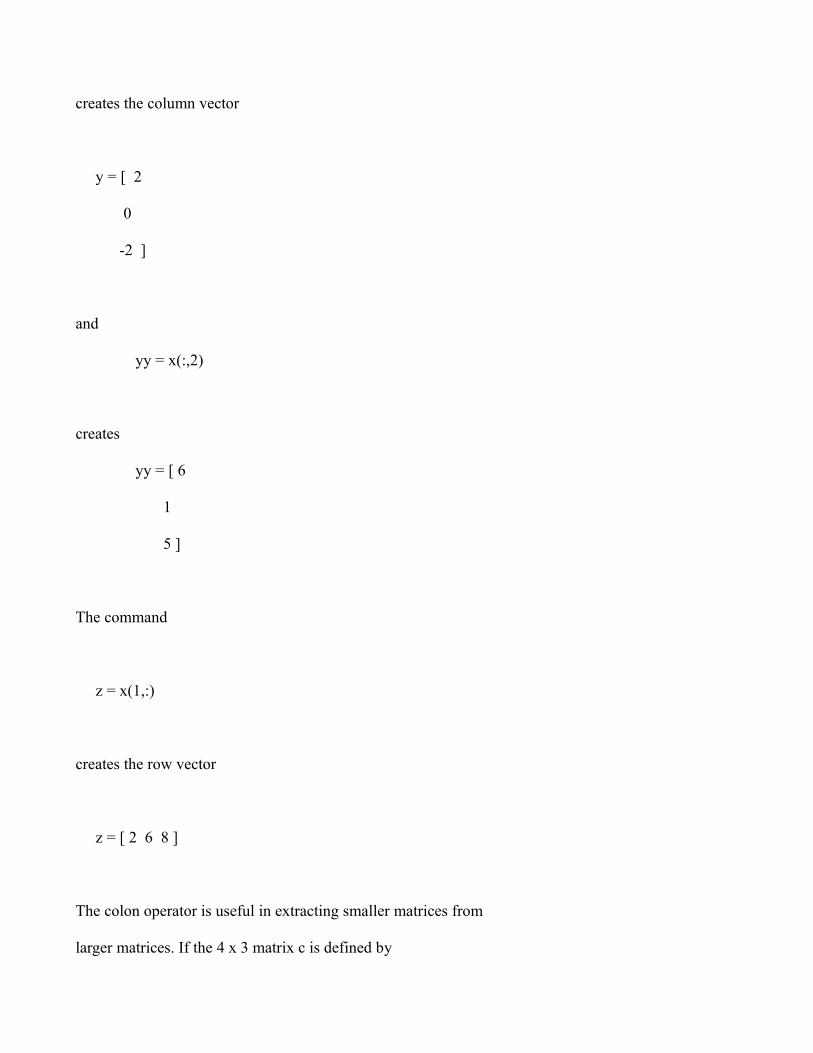
creates the column vector

y = [ 2

0

-2 ]

and

yy = x(:,2)

creates

yy = [ 6

1

5 ]

The command

z = x(1,:)

creates the row vector

z = [ 2 6 8 ]

The colon operator is useful in extracting smaller matrices from

larger matrices. If the 4 x 3 matrix c is defined by

c = [ -1 0 0

1 1 0

1 -1 0

0 0 2 ]

Then

d1 = c(:,2:3)

creates a matrix for which all elements of the rows from the 2nd

and third columns are used. The result is a 4 x 2 matrix

d1 = [ 0 0

1 0

-1 0

0 2 ]

The command

d2 = c(3:4,1:2)

creates a 2 x 2 matrix in which the rows are defined by the 3rd and

4th row of c and the columns are defined by the 1st and 2nd columns

of the matrix, c.

d2 = [ 1 -1

0 0 ]

USING THE CLEAR COMMANDS

Before quitting this session of 'matlab', note the use of the

commands 'clear' and 'clc'. Note that 'clc' simply clears the

screen, but does not clear or erase any matrices that have been

defined. The command 'clear' erase or removes matrices from your

workspace. Use this command with care. NOTE THE COMMAND 'CLEAR'

WITHOUT ANY MODIFYING STRING WILL ERASE ALL MATRICES IN YOUR

WORKSPACE.

PROBLEMS

Define the 5 x 4 matrix, g.

g = [ 0.6 1.5 2.3 -0.5

8.2 0.5 -0.1 -2.0

5.7 8.2 9.0 1.5

0.5 0.5 2.4 0.5

1.2 -2.3 -4.5 0.5 ]

Determine the content and size of the following matrices and check

your results for content and size using 'matlab'.

1. a = g(:,2)

2. b = g(4,:)

3. c = [10:15]

4. d = [4:9;1:6]

5. e = [-5,5]

6. f= [1.0:-.2:0.0]

7. t1 = g(4:5,1:3)

8. t2 = g(1:2:5,:)

New commands in this lesson:

plot(x,y) creates a Cartesian plot of the vectors x & y

plot(y) creates a plot of y vs. the numerical values of the

elements in the y-vector.

semilogx(x,y) plots log(x) vs y

semilogy(x,y) plots x vs log(y)

loglog(x,y) plots log(x) vs log(y)

grid creates a grid on the graphics plot

title('text') places a title at top of graphics plot

xlabel('text') writes 'text' beneath the x-axis of a plot

ylabel('text') writes 'text' beside the y-axis of a plot

text(x,y,'text') writes 'text' at the location (x,y)

text(x,y,'text','sc') writes 'text' at point x,y assuming

lower left corner is (0,0) and upper

right corner is (1,1).

polar(theta,r) creates a polar plot of the vectors r & theta

where theta is in radians.

bar(x) creates a bar graph of the vector x. (Note also

the command stairs(x).)

bar(x,y) creates a bar-graph of the elements of the vector y,

locating the bars according to the vector elements

of 'x'. (Note also the command stairs(x,y).)

CARTESIAN OR X-Y PLOTS

One of 'matlab' most powerful features is the ability to

create graphic plots. Here we introduce the elementary ideas for

simply presenting a graphic plot of two vectors. More complicated

and powerful ideas with graphics can be found in the 'matlab'

documentation.

A Cartesian or orthogonal x,y plot is based on plotting the

x,y data pairs from the specified vectors. Clearly, the vectors x

and y must have the same number of elements. Imagine that you wish

to plot the function ex for values of x from 0 to 2.

x = 0:.1:2;

y = exp(x);

plot(x,y)

NOTE: The use of selected functions such as exp() and sin() will be

used in these tutorials without explanation if they take on an

unambiguous meaning consistent with past experience. Here it is

observed that operating on a matrix with these functions simply

creates a matrix in which the elements are based on applying the

function to each corresponding element of the argument.

Of course the symbols x,y are arbitrary. If we wanted to plot

temperature on the ordinate and time on the abscissa, and vectors

for temperature and time were loaded in 'matlab', the command would

be

plot(time,temperature)

Notice that the command plot(x,y) opens a graphics window. If you

now execute the command 'grid', the graphics window is redrawn.

(Note you move the cursor to the command window before typing new

commands.) To avoid redrawing the window, you may use the line

continuation ellipsis. Consider

plot(x,y),...

grid,...

title('Exponential Function'),...

xlabel('x'),...

ylabel('exp(x)'),

text(.6,.4,' y = exp(x)','sc')

Note that if you make a mistake in typing a series of lines of

code, such as the above, the use of line continuation can be

frustrating. In a future lesson, we will learn how to create batch

files (called '.m' files) for executing a series of 'matlab'

commands. This approach gives you better opportunity to return to

the command string and edit errors that have been created.

Having defined the vectors x and y, construct semilog and log-

log plots using these or other vectors you may wish to create. Note

in particular what occurs when a logarithmic scale is selected for

a vector that has negative or zero elements. Here, the vector x has

a zero element (x(1)=0). The logarithm of zero or any negative

number is undefined and the x,y data pair for which a zero or

negative number occurs is discarded and a warning message provided.

Try the commands plot(x) and plot(y) to ensure you understand

how they differ from plot(x,y).

Notice that 'matlab' draws a straight line between the data-

pairs. If you desire to see a relatively smooth curve drawn for a

rapidly changing function, you must include a number of data

points. For example, consider the trigonometric function, sin(x1)

(x1 is selected as the argument here to distinguish it from the

vector 'x' that was defined earlier. )

Plot sin(x1) over the limits 0 <= x1 <= pi. First define x1

with 5 elements,

x1 = 0 : pi/4 : pi

y1 = sin(x1)

plot(x1,y1)

Now, repeat this after defining a new vector for x1 and y1 with 21

elements. (Note the use of the semicolon here to prevent the

printing and scrolling on the monitor screen of a vector or matrix

with a large number of elements!)

x1 = 0 : .05*pi : pi ;

y1 =sin(x1);

plot(x1,y1)

POLAR PLOTS

Polar plots are constructed much the same way as are Cartesian

x-y plots; however, the arguments are the angle 'theta' in radians

measured CCW from the horizontal (positive-x) axis, and the length

of the radius vector extended from the origin along this angle.

Polar plots do not allow the labeling of axes; however, notice that

the scale for the radius vector is presented along the vertical and

when the 'grid' command is used the angles-grid is presented in 15-

degree segments. The 'title' command and the 'text' commands are

functional with polar plots.

angle = 0:.1*pi:3*pi;

radius = exp(angle/20);

polar(angle,radius),...

title('An Example Polar Plot'),...

grid

Note that the angles may exceed one revolution of 2*pi.

BAR GRAPHS

To observe how 'matlab' creates a bargraph, return to the

vectors x,y that were defined earlier. Create bar and stair graphs

using these or other vectors you may define. Of course the 'title'

and 'text' commands can be used with bar and stair graphs.

bar(x,y) and bar(y)

stair (x,y) and stair(y)

MULTIPLE PLOTS

More than a single graph can be presented on one graphic plot.

One common way to accomplish this is hold the graphics window open

with the 'hold' command and execute a subsequent plotting command.

x1=0:.05*pi:pi;

y1=sin(x1);

plot(x1,y1)

hold

y2=cos(x1);

plot(x1,y2)

The "hold" command will remain active until you turn it off with

the command 'hold off'.

You can create multiple graphs by using multiple arguments.

In addition to the vectors x,y created earlier, create the vectors

a,b and plot both vector sets simultaneously as follows.

a = 1 : .1 : 3;

b = 10*exp(-a);

plot(x,y,a,b)

Multiple plots can be accomplished also by using matrices

rather than simple vectors in the argument. If the arguments of

the 'plot' command are matrices, the COLUMNS of y are plotted on

the ordinate against the COLUMNS of x on the abscissa. Note that x

and y must be of the same order! If y is a matrix and x is a

vector, the rows or columns of y are plotted against the elements

of x. In this instance, the number of rows OR columns in the matrix

must correspond to the number of elements in 'x'. The matrix 'x'

can be a row or a column vector!

Recall the row vectors 'x' and 'y' defined earlier. Augment

the row vector 'y' to create the 2-row matrix, yy.

yy=[y;exp(1.2*x)];

plot(x,yy)

PLOTTING DATA POINTS & OTHER FANCY STUFF

Matlab connects a straight line between the data pairs

described by the vectors used in the 'print' command. You may wish

to present data points and omit any connecting lines between these

points. Data points can be described by a variety of characters

( . , + , * , o and x .) The following command plots the x,y data

as a "curve" of connected straight lines and in addition places an

'o' character at each of the x1,y1 data pairs.

plot(x,y,x1,y1,'o')

Lines can be colored and they can be broken to make

distinctions among more than one line. Colored lines are effective

on the color monitor and color printers or plotters. Colors are

useless on the common printers used on this network. Colors are

denoted in 'matlab' by the symbols r(red), g(green), b(blue),

w(white) and i(invisible). The following command plots the x,y

data in red solid line and the r,s data in broken green line.

plot(x,y,'r',r,s,'--g')

PRINTING GRAPHIC PLOTS

Executing the 'print' command will send the contents of the

current graphics widow to the local printer.

You may wish to save in a graphics file, a plot you have

created. To do so, simply append to the 'print' command the name

of the file. The command

print filename

will store the contents of the graphics window in the file titled

'filename.ps' in a format called postscript. You need not include

the .ps suffix, as matlab will do this. When you list the files

in your matlab directory, it is convenient to identify any graphics

files by simply looking for the files with the .ps suffix. If

you desire to print one of these postscript files, you can

conveniently "drag and drop" the file from the file-manager window

into the printer icon.

Commands introduced in this lesson:

max(x) returns the maximum value of the elements in a

vector or if x is a matrix, returns a row vector

whose elements are the maximum values from each

respective column of the matrix.

min (x) returns the minimum of x (see max(x) for details).

mean(x) returns the mean value of the elements of a vector

or if x is a matrix, returns a row vector whose

elements are the mean value of the elements from

each column of the matrix.

median(x) same as mean(x), only returns the median value.

sum(x) returns the sum of the elements of a vector or if x

is a matrix, returns the sum of the elements from

each respective column of the matrix.

prod(x) same as sum(x), only returns the product of

elements.

std(x) returns the standard deviation of the elements of a

vector or if x is a matrix, a row vector whose

elements are the standard deviations of each

column of the matrix.

sort(x) sorts the values in the vector x or the columns of

a matrix and places them in ascending order. Note

that this command will destroy any association that

may exist between the elements in a row of matrix x.

hist(x) plots a histogram of the elements of vector, x. Ten

bins are scaled based on the max and min values.

hist(x,n) plots a histogram with 'n' bins scaled between the

max and min values of the elements.

hist((x(:,2)) plots a histogram of the elements of the 2nd

column from the matrix x.

The 'matlab' commands introduced in this lesson perform

simple statistical calculations that are mostly self-explanatory.

A simple series of examples are illustrated below. Note that

'matlab' treats each COLUMN OF A MATRIX as a unique set of "data",

however, vectors can be row or column format. Begin the exercise

by creating a 12x3 matrix that represents a time history of two

stochastic temperature measurements.

Load these data into a matrix called 'timtemp.dat' using an

editor to build an ASCII file.

Time(sec) Temp-T1(K) Temp-T2(K)

0.0 306 125

1.0 305 121

2.0 312 123

3.0 309 122

4.0 308 124

5.0 299 129

6.0 311 122

7.0 303 122

8.0 306 123

9.0 303 127

10.0 306 124

11.0 304 123

Execute the commands at the beginning of the lesson above and

observe the results. Note that when the argument is 'timtemp', a

matrix, the result is a 1x3 vector. For example, the command

M = max(timtemp)

gives

M = 11 312 129

If the argument is a single column from the matrix, the

command identifies the particular column desired. The command

M2 = max(timtemp(:,2))

gives

M2 = 312

If the variance of a set of data in a column of the matrix is

desired, the standard deviation is squared. The command

T1_var = (std(timtemp(:,2)))^2

gives

T1_var = 13.2727

If the standard deviation of the matrix of data is found using

STDDEV = std(timtemp)

gives

STDDEV = 3.6056 3.6432 2.3012

Note that the command

VAR = STDDEV^2

is not acceptable; however, the command

VAR = STDDEV.^2

is acceptable, creating the results,

VAR = 13.0000 13.2727 5.2955

USING m-FILES - SCRATCH and FUNCTION FILES

Sometimes it is convenient to write a number of lines of

'matlab' code before executing the commands. We have seen how this

can be accomplished using the line continuation ellipsis; however,

it was noted in this approach that any mistake in the code required

the entire string to be entered again. Using an m-file we can

write a number of lines of 'matlab' code and store it in a file

whose name we select with the suffix '.m' added. Subsequently the

command string or file content can be executed by invoking the name

of the file while in 'matlab'. This application is called a

SCRATCH FILE.

On occasion it is convenient to express a function in 'matlab'

rather than calculating or defining a particular matrix. The many

'matlab' stored functions such as sin(x) and log(x) are examples of

functions. We can write functions of our definition to evaluate

parameters of our particular interest. This application of m-files

is called FUNCTION FILES.

SCRATCH FILES

A scratch file must be prepared in a text editor in ASCII

format and stored in the directory from which you invoked the

command to download 'matlab'. The name can be any legitimate file

name with the '.m' suffix.

As an example, suppose we wish to prepare a x-y plot of the

function

y = e-x/10 sin(x) 0 x ø 10 .

To accomplish this using a scratch ".m-file", we will call the file

'explot.m'. Open the file in a text editor and type the code

below. (Note the use of the '%' in line 1 below to create a

comment. Any text or commands typed on a line after the'%' will be

treated as a comment and ignored in the executable code.)

% A scratch m-file to plot exp(-x/10)sin(x)

x = [ 0:.2:10 ];

y = exp(-x/10) .* sin(x);

plot(x,y),...

title('EXPONENTIAL DAMPED SINE FUNCTION'),...

xlabel('x'),...

ylabel('y'),...

text(.6,.7,'y = exp(-x/10)*sin(x)','sc')

Store this file under the name 'explot.m in your 'matlab'

directory. Now when you are in 'matlab', any time you type the

command 'explot' the x-y plot of the damped exponential sine

function will appear.

FUNCTION FILES

Suppose that you wish to have in your 'matlab' workspace a

function that calculates the sine of the angle when the argument is

in degrees. The matlab function sin(x) requires that x be in

radians. A function can be written that use the 'matlab' sin(x)

function, where x is in radians, to accomplish the objective of

calculating the sine of an argument expressed in degrees. Again,

as in the case of the scratch file, we must prepare the file in

ASCII format using a text editor, and we must add the suffix '.m'

to the file. HERE THE NAME OF THE FILE MUST BE THE NAME OF THE

FUNCTION.

The following code will accomplish our objective. Note that the

first line must always begin with the word "function" followed by

the name of the function expressed as " y = function-name". Here

the function name is "sind(x)". This is the name by which we will

call for the function once it is stored.

function y = sind(x)

% This function calculates the sine when the argument is degrees

% Note that array multiplication and division allows this to

% operate on scalars, vectors and matrices.

y = sin( x .* pi ./ 180 )

Again, note the rule in writing the function is to express in the

first line of the file the word 'function', followed by

y = function call,

here 'sind' with the function argument in parentheses, 'x' is the

function call. Thus,

function y=sind(x)

Now every time we type sind(x) in 'matlab', it will return the

value of the sine function calculated under the assumption that x

is in degrees. Of course any matrix or expression involving a

matrix can be written in the argument.

ALGEBRAIC OPERATIONS IN MATLAB

Scalar Calculations. The common arithmetic operators used in

spreadsheets and programming languages such as BASIC are used in

'matlab'. In addition a distinction is made between right and left

division. The arithmetic operators are

+ addition

- subtraction

* multiplication

/ right division (a/b means a ÷ b)

\ left division (a\b means b ÷ a)

^ exponentiation

When a single line of code includes more than one of these

operators the precedence or order of the calculations follows the

below order:

Precedence Operation

1 parentheses

2 exponentiation, left to right

3 multiplication and division, left right

4 addition and subtraction, left right

These rules are applied to scalar quantities (i.e., 1x1 matrices)

in the ordinary manner. (Below we will discover that nonscalar

matrices require additional rules for the application of these

operators!!) For example,

3*4 executed in 'matlab' gives

ans=12

4/5 executed in 'matlab' gives

ans=.8000

4\5 executed in 'matlab' gives

ans=1.2500

x = pi/2; y = sin(x) executed in 'matlab' gives

y = 1

z = 0; w = exp(4*z)/5 executed in 'matlab" gives

z= .2000

Note that many programmers will prefer to write the expression for

w above in the format

w = (exp(4*x))/5

which gives the same result and is sometimes less confusing when

the string of arithmetic operations is long. Using 'matlab', carry

out some simple arithmetic operations with scalars you define. In

doing so utilize the 'matlab' functions sqrt(x), abs(s), sin(x),

asin(x), atan(x), atan2(x), log(x), and log10(x) as well as exp(x).

Many other functions are available in 'matlab' and can be found in

the documentation.

Matrix Calculations. Because matrices are made up of a number

of elements and not a single number (except for the 1x1 scalar

matrix), the ordinary rules of commutative, associative and

distributive operations in arithmetic do not always follow.

Moreover, a number of important but common-sense rules will prevail

in matrix algebra and 'matlab' when dealing with nonscalar

quantities.

Addition and Subtraction of Matrices. Only matrices of the SAME

ORDER can be added or subtracted. When two matrices of the same

order are added or subtracted in matrix algebra, the individual

elements are added or subtracted. Thus the distributive rule

applies.

A + B = B + A and A - B = B - A

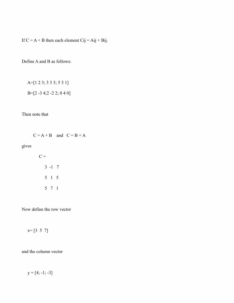
If C = A + B then each element Cij = Aij + Bij.

Define A and B as follows:

A=[1 2 3; 3 3 3; 5 3 1]

B=[2 -3 4;2 -2 2; 0 4 0]

Then note that

C = A + B and C = B + A

gives

C =

3 -1 7

5 1 5

5 7 1

Now define the row vector

x= [3 5 7]

and the column vector

y = [4; -1; -3]

Note that the operation

z = x + y

is not valid! It is not valid because the two matrices do not have

the same order. (x is a 1x3 matrix and y is a 3x1 matrix.) Adding

any number of 1x1 matrices or scalars is permissible and follows

the ordinary rules of arithmetic because the 1x1 matrix is a

scalar. Adding two vectors is permissible so long as each is a row

vector (1xn matrix) or column vector (nx1 matrix). Of course any

number of vectors can be added or subtracted, the result being the

arithmetic sum of the individual elements in the column or row

vectors. Square matrices can always be added or subtracted so long

as they are of the same order. A 4x4 square matrix can not be added

to a 3x3 square matrix, because they are not of the same order,

although both matrices are square.

Multiplication of Matrices. Matrix multiplication, though straight-

forward in definition, is more complex than arithmetic

multiplication because each matrix contains a number of elements.

Recall that with vector multiplication, the existence of a number

of elements in the vector resulted in two concepts of

multiplication, the scalar product and the vector product. Matrix

multiplication has its array of special rules as well.

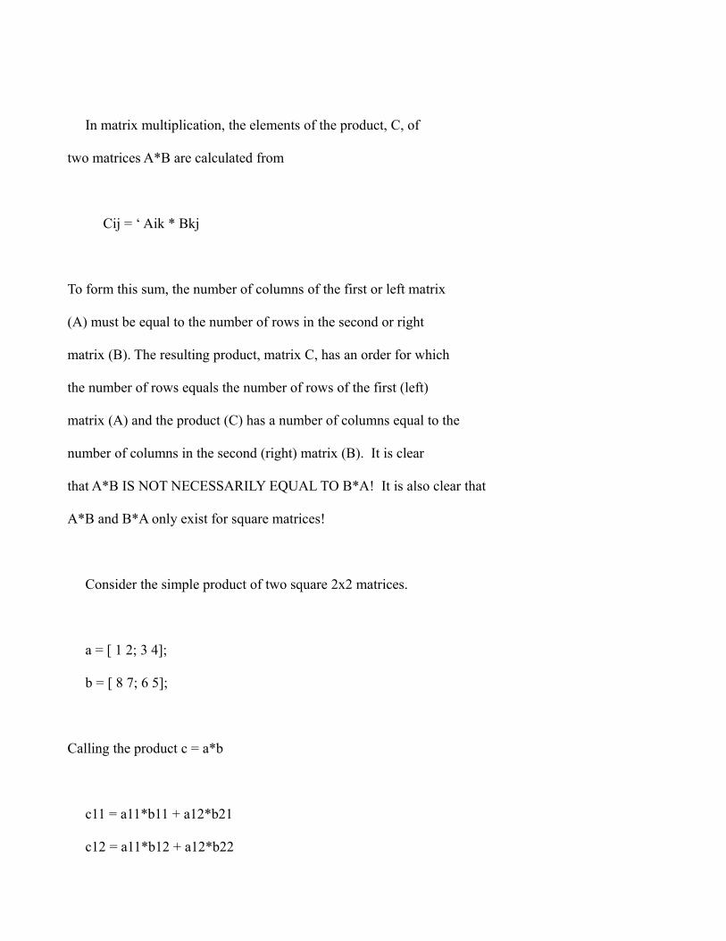
In matrix multiplication, the elements of the product, C, of

two matrices A*B are calculated from

Cij = ‘ Aik * Bkj

To form this sum, the number of columns of the first or left matrix

(A) must be equal to the number of rows in the second or right

matrix (B). The resulting product, matrix C, has an order for which

the number of rows equals the number of rows of the first (left)

matrix (A) and the product (C) has a number of columns equal to the

number of columns in the second (right) matrix (B). It is clear

that A*B IS NOT NECESSARILY EQUAL TO B*A! It is also clear that

A*B and B*A only exist for square matrices!

Consider the simple product of two square 2x2 matrices.

a = [ 1 2; 3 4];

b = [ 8 7; 6 5];

Calling the product c = a*b

c11 = a11*b11 + a12*b21

c12 = a11*b12 + a12*b22

c21 = a21*b11 + a22*b21

c22 = a21*b12 + a22*b22

Carry out the calculations by hand and verify the result using

'matlab'. Next, consider the following matrix product of a 3x2

matrix X and a 2x4 matrix Y.

X = [2 3 ; 4 -1 ; 0 7];

Y = [5 -6 7 2 ; 1 2 3 6];

First, note that the matrix product X*Y exists because X has the

same number of columns (2) as Y has rows (2). (Note that Y*X does

NOT exist!) If the product of X*Y is called C, the matrix C must

be a 3x4 matrix. Again, carry out the calculations by hand and

verify the result using 'matlab'.

Note that the PRODUCT OF A SCALAR AND A MATRIX is a matrix in

which every element of the matrix has been multiplied by the

scalar. Verify this by recalling the matrix X defined above, and

carry out the product 3*X on 'matlab'. (Note that this can be

written X*3 as well as 3*X, because quantity '3' is scalar.)

ARRAY PRODUCTS

Recall that addition and subtraction of matrices involved

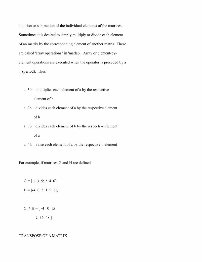
addition or subtraction of the individual elements of the matrices.

Sometimes it is desired to simply multiply or divide each element

of an matrix by the corresponding element of another matrix. These

are called 'array operations" in 'matlab'. Array or element-by-

element operations are executed when the operator is preceded by a

'.' (period). Thus

a .* b multiplies each element of a by the respective

element of b

a ./ b divides each element of a by the respective element

of b

a .\ b divides each element of b by the respective element

of a

a .^ b raise each element of a by the respective b element

For example, if matrices G and H are defined

G = [ 1 3 5; 2 4 6];

H = [-4 0 3; 1 9 8];

G .* H = [ -4 0 15

2 36 48 ]

TRANSPOSE OF A MATRIX

The transpose of a matrix is obtained by interchanging the

rows and columns. The 'matlab' operator that creates the transpose

is the single quotation mark, '. Recalling the matrix G

G' = [ 1 2

3 4

5 6 ]

Note that the transpose of a m x n matrix creates a n x m matrix.

One of the most useful operations involving the transpose is that

of creating a column vector from a row vector, or a row vector from

a column vector.

INNER (SCALAR) PRODUCT OF TWO VECTORS

The scalar or inner product of two row vectors, G1 and G2 is

found as follows. Create the row vectors for this example by

decomposing the matrix G defined above.

G1 = G(1,:)

G2 = G(2,:)

Then the inner product of the 1x3 row vector G1 and the 1x3 row

vector G2 is

G1 * G2' = 44

Verify this result by carrying out the operations on 'matlab'.

If the two vectors are each column vectors, then the inner

product must be formed by the matrix product of the transpose of a

column vector times a column vector, thus creating an operation in

which a 1 x n matrix is multiplied with a n x 1 matrix.

In summary, note that the inner product must always be the

product of a row vector times a column vector.

OUTER PRODUCT OF TWO VECTORS

If two row vectors exist, G1 and G2 as defined above, the

outer product is simply

G1' * G2 {Note G1' is 3x1 and G2 is 1x3}

and the result is a square matrix in contrast to the scalar result

for the inner product. DON'T CONFUSE THE OUTER PRODUCT WITH THE

VECTOR PRODUCT IN MECHANICS! If the two vectors are column

vectors, the outer product must be formed by the product of one

vector times the transpose of the second!

OTHER OPERATIONS ON MATRICES

As noted above, many functions that exist can be applied

directly to a matrix by simply allowing the function to operate on

each element of the matrix array. This is true for the

trigonometric functions and their inverse. It is true also for the

exponential function, ex, exp(), and the logarithmic functions,

log() and log10().

Exponential operations (using ^) on matrices are quite

different from their use with scalars. If W is a square matrix

W^2 implies W*W which is quite different from W.*W. Be certain of

your intent before raising a matrix to an exponential power. Of

course W^2 only exists if W is a square matrix.

SPECIAL MATRICES

A number of special functions exist in 'matlab' to create

special or unusual matrices. For example, matrices with element

values of zero or 1 are sometimes useful.

zeros(4)

creates a square matrix (4 x 4) whose elements are zero.

zeros(3,2)

creates a 3 row, 2 column matrix of zeros.

Similarly the commands ones(4) creates a 4 x 4 square matrix

whose elements are 1's and 'ones(3,2)' creates a 3x2 matrix whose

elements are 1's.

If a m x n matrix, say A, already exists, the command

'ones(A)' creates an m x n matrix of 1's. The command 'zeros(A)'

creates an mxn matrix of 0's. Note that these commands do not

alter the previously defined matrix A, which is only a basis for

the size of the matrix created by commands zeros() and ones().

The identity matrix is a square matrix with 1's on the

diagonal and 0's off the diagonal. Thus a 4x4 identity matrix, a,

is

a=[1 0 0 0

0 1 0 0

0 0 1 0

0 0 0 1]

This matrix can be created with the 'eye' function. Thus,

a = eye(4)

The 'eye' function will create non-square matrices. Thus

eye(3,2)

creates

1 0

0 1

0 0

and

eye(2,3)

creates

1 0 0

0 1 0

PRACTICE

1. The first four terms of the fourier series for the square wave

whose amplitude is 5 and whose period is 2ƒ is

y = (20/ƒ)[sinx + (1/3)sin3x + (1/5)sin5x + (1/7)sin7x)]

Calculate this series, term by term, and plot the results for each

partial sum.