arX

iv:q

uant

-ph/

9608

004v

1 5

Aug

199

6

A C++ library using quantum trajectories

to solve quantum master equations

Rudiger Schack∗(a,b)

and Todd A. Brun†(b)

(a)Department of Mathematics, Royal Holloway, University of London

Egham, Surrey TW20 0EX, England

(b)Department of Physics, Queen Mary and Westfield College

University of London, London E1 4NS, England

July 18, 1996

Abstract

Quantum trajectory methods can be used for a wide range of open quantum

systems to solve the master equation by unraveling the density operator evolution

into individual stochastic trajectories in Hilbert space. This C++ class library of-

fers a choice of integration algorithms for three important unravelings of the master

equation. Different physical systems are modeled by different Hamiltonians and en-

vironment operators. The program achieves flexibility and user friendliness, without

sacrificing execution speed, through the way it represents operators and states in

Hilbert space. Primary operators, implemented in the form of simple routines acting

on single degrees of freedom, can be used to build up arbitrarily complex operators

in product Hilbert spaces with arbitrary numbers of components. Standard alge-

braic notation is used to build operators and to perform arithmetic operations on

operators and states. States can be represented in a local moving basis, often lead-

ing to dramatic savings of computing resources. The state and operator classes are

very general and can be used independently of the quantum trajectory algorithms.

Only a rudimentary knowledge of C++ is required to use this package.

∗Email: r.schack@rhbnc.ac.uk†Email: t.brun@qmw.ac.uk

1

Program Summary

Title of program: Quantum trajectory class library

Program obtainable from: http://galisteo.ma.rhbnc.ac.uk/applied/QSD.html and the au-thors.

Licensing provisions : none

Operating systems under which the program has been tested : UNIX (Gnu g++), DOS(Turbo C++), VMS (DEC C++)

Programming language used : C++

Memory required to execute with typical data: 1MByte

Has the code been vectorized? : no

No. of lines in distributed program, including test data, etc.: 8000

Keywords: open quantum system, master equation, Hilbert space, quantum trajectories,unraveling, stochastic simulation, quantum computation, quantum optics, quantum statediffusion, quantum jumps, Monte Carlo wavefunction

Nature of physical problem:Open quantum systems, i.e., systems whose interaction with the environment can notbe neglected, occur in a variety of contexts. Examples are quantum optics, atomic andmolecular physics, and quantum computers. If the time evolution of the system is ap-proximately Markovian, it can be described by a master equation of Lindblad form [1],a first order differential equation for the density operator. Solving the master equationis the principal purpose of the program. Since the state and operator classes are verygeneral, they can be used in any physical problem involving Hilbert spaces with severaldegrees of freedom.

Method of solution:By analogy with the solution of a Fokker-Planck equation by numerical simulation of thecorresponding stochastic differential equation, a master equation can be solved by simu-lating the stochastic evolution of a vector in Hilbert space. The correspondence betweenmaster equation and stochastic equation is not unique: there are many ways to unravel

the master equation into stochastic quantum trajectories. The program implements threesuch unravelings, known as the “quantum state diffusion method (QSD)” [2], the “quan-tum jump method” [3–5], and the “orthogonal jump method”[6]. The phenomenon ofphase-space localization [7,8] is exploited numerically by representing quantum states ina local moving basis obtained by applying the coherent-state displacement operator to theusual harmonic-oscillator basis, often leading to dramatic savings of computing resources.

Unusual features of the program:It is worth emphasizing the effortless way in which operators and states in product Hilbertspaces are represented. Primary operators implemented in the form of simple routinesacting on single degrees of freedom can be used to build up arbitrarily complex operatorsin product Hilbert spaces with arbitrary numbers of components. Building operators, per-forming arithmetic operations on operators and states, and applying operators to states isdone using standard algebraic notation. This program structure has been made possible

2

by systematically implementing object-oriented programming concepts such as inheri-tance, concepts which are not (yet) widely used in computational physics. Encapsulationof program modules makes it easy to add new basic operators, alternative unravelings ofthe master equation, or different integration algorithms.

Typical running time:The running time depends on the complexity of the problem, the integration time, andthe number of trajectories required. A typical running time for a simple problem is a fewminutes. There is no upper limit.

References :[1] G. Lindblad, Commun. Math. Phys. 48, 119 (1976).[2] N. Gisin and I. C. Percival, J. Phys. A 25, 5677 (1992).[3] H. J. Carmichael, An Open Systems Approach to Quantum Optics (Springer, Berlin,1993).[4] J. Dalibard, Y. Castin, and K. Mølmer, Phys. Rev. Lett. 68, 580 (1992).[5] C. W. Gardiner, A. S. Parkins, and P. Zoller, Phys. Rev. A 46, 4363 (1992).[6] L. Diosi, Phys. Lett. A 114, 451 (1986).[7] T. Steimle, G. Alber, and I. C. Percival, J. Phys. A 28, L491 (1995).[8] R. Schack, T. A. Brun, and I. C. Percival, J. Phys. A 28, 5401 (1995).

Long Write-Up

1 Introduction

For many quantum systems of current interest it is no longer possible to neglect theinteractions with the environment. Those so-called open quantum systems occur in avariety of contexts including quantum optics, atomic and molecular physics, and quantumcomputers. Open quantum systems can often be described by a master equation [1], afirst-order differential equation for the density operator, in which the internal dynamicsof the system is represented by the system Hamiltonian H , which is a Hermitian Hilbert-space operator, and the interaction with the environment is represented by one or moreLindblad operators Lj which are not necessarily Hermitian.

By analogy with the solution of a Fokker-Planck equation by numerical simulationof the corresponding stochastic differential equation (or Langevin equation), a masterequation can be solved by simulating the stochastic evolution of a vector in Hilbert space.The correspondence between master equation and stochastic equation is not unique; thereare many ways to unravel the master equation into stochastic quantum trajectories [2, 3,4, 5, 6, 7].

The main challenge of this software project was to develop a general program flexibleenough to accommodate different integration algorithms and unravelings of the masterequation, as well as the vast range of possible physical systems. In particular, we wanted tomake it easy to add new algorithms and unravelings, and we wanted a program capableof dealing with arbitrary Hamiltonian and Lindblad operators in Hilbert spaces withan arbitrary number of degrees of freedom. This task turned out to be ideal for theapplication of object-oriented programming. We chose the C++ language both becauseof its wide availability and because it allowed us to use standard mathematical notationfor Hilbert-space operations by overloading algebraic operators like ‘+’ and ‘∗’.

3

The core of the program are the C++ classes State and Operator, which representstate vectors and operators in Hilbert space. Because of the object-oriented features ofC++, it is possible to hide the implementation details of these classes completely from theclasses dealing with the simulation of quantum trajectories. These implementation detailsneed not to be known either by a user of the program who wants to choose the quantumoperators defining the physical problem of interest or by a programmer who wants to adda new unraveling of the master equation to the software. A welcome side effect of thisencapsulation is that the State and Operator classes can be used independently of therest of the code. They should prove useful in many numerical schemes involving Hilbertspaces for systems with several degrees of freedom.

Many Hamiltonian and Lindblad operators can be written as sums of products ofsimple operators acting on a single degree of freedom. Here is an example of a Hamiltonianoperator coupling a two-level atom (with raising and lowering operators σ+ and σ−) toan electromagnetic field mode (with annihilation and creation operators a and a†):

H = g(

σ+a + σ−a†)

, (1)

where the parameter g is the coupling strength. In the following code segment, the atomicand field degrees of freedom are labeled 0 and 1, respectively. The Hamiltonian is definedin terms of the predefined primary operators SigmaPlus and AnnihilationOperator

using standard algebraic notation. The class AdaptiveStep is a stepper routine advancingthe quantum trajectory by a single time step.

double g = 0.5;

SigmaPlus Sp(0); // operates on the 1st degree of freedom

AnnihilationOperator A(1); // operates on the 2nd degree of freedom

Operator Sm = Sp.hc(); // Hermitian conjugate

Operator Ac = A.hc();

Operator H = g*( Sp*A + Sm*Ac ); // Hamiltonian

...

AdaptiveStep theStepper(..., H, ...); // ... denotes further arguments

The important feature illustrated by this example is that the stepper routine is passedan object of type Operator without any reference to details like the number of degrees offreedom. All the stepper needs to know is that operators can be added, multiplied, etc.,and that they can be applied to state vectors.

Internally, the primary operators SigmaPlus and AnnihilationOperator are repre-sented as simple loops acting on a single-degree-of-freedom state vector. An instance ofthe more general Operator class is represented by a stack that indicates which primaryoperators are used and the operations by which they are combined. For example, thesequence of steps executed by the program when the operator H defined above is appliedto a state |ψ〉 is summarized in the expression

H|ψ〉 = g(

σ+(a|ψ〉) + σ−(a†|ψ〉))

, (2)

in which the elementary steps are applying a primary operator to a state, adding twostates, and multiplying a state by a scalar. It is clear from this example that a differentgrouping of the terms in the expression for H could lead to inefficient code. This will bediscussed in Sec. 4.1.2.

4

2 Quantum trajectories

2.1 Master equations

An open quantum system cannot be described by a Hilbert-space vector |ψ〉 evolvingaccording to the Schrodinger equation; instead, the state must be described by a densityoperator ρ whose time evolution generally does not follow any simple law. Fortunately itturns out that for a large class of systems the time evolution of the density operator ρ isMarkovian to an excellent approximation, i.e., the rate of change of ρ at time t, dρ/dt,depends only on ρ(t), not on the value of ρ at any earlier time. It has been shown thatunder the Markov approximation the density operator of any open quantum system obeysa master equation of Lindblad form [1]

d

dtρ = − i

h[H, ρ] +

∑

j

(

Lj ρL†j −

1

2L†jLjρ−

1

2ρL†

jLj

)

, (3)

where H is the system Hamiltonian and the Lj are the Lindblad operators representingthe interaction with the environment.

In many cases, no analytical methods for the solution of the master equation areknown; one has to use numerical methods. But even a numerical solution of the masterequation can be very hard. If a state requires D basis vectors in Hilbert space to representit, the corresponding density operator will require D2 − 1 real numbers; this can oftenbe too large for even the most powerful machines to handle, particularly if the systeminvolves more than one degree of freedom.

This problem can be overcome by unraveling the density operator evolution into quan-

tum trajectories [2, 3, 4, 5, 6, 7]. Since quantum trajectories represent the system as astate vector rather than a density operator, they often have a numerical advantage oversolving the master equation directly, even though one has to average over many quantumtrajectories to recover the solution of the master equation. A single quantum trajectorycan give an excellent, albeit qualitative, picture of a single experimental run.

2.2 Unravelings

The three unravelings of the master equation currently implemented are given by thefollowing three nonlinear stochastic differential equation for a normalized state vector|ψ〉:(i) the quantum state diffusion (QSD) equation [3]

|dψ〉 = − i

hH |ψ〉dt+

∑

j

(

〈L†j〉ψLj −

1

2L†jLj −

1

2〈L†

j〉ψ〈Lj〉ψ)

|ψ〉dt

+∑

j

(

Lj − 〈Lj〉ψ)

|ψ〉dξj , (4)

(ii) the quantum jump equation [4, 5, 6]

|dψ〉 = − i

hH |ψ〉dt+

∑

j

(

1

2〈L†

jLj〉ψ − 1

2L†jLj

)

|ψ〉dt

+∑

j

Lj√

〈L†jLj〉ψ

− 1

|ψ〉dNj , (5)

5

and (iii) the orthogonal jump equation [2, 7]

|dψ〉 = − i

hH |ψ〉dt+

∑

j

(

〈L†j〉ψLj −

1

2L†jLj +

1

2〈L†

jLj〉ψ − 〈L†j〉ψ〈Lj〉ψ

)

|ψ〉dt

+∑

j

Lj − 〈Lj〉ψ√

〈L†jLj〉ψ − 〈L†

j〉ψ〈Lj〉ψ− 1

|ψ〉dNj . (6)

The first sum in each of these equations represents the deterministic drift of the statevector due to the environment, and the second sum the random fluctuations. Angularbrackets denote the quantum expectation 〈G〉ψ = 〈ψ|G|ψ〉 of the operator G in the state|ψ〉. The dξj are independent complex differential Gaussian random variables satisfyingthe conditions

Mdξj = Mdξidξj = 0 , Mdξ∗i dξj = δijdt , (7)

where M denotes the ensemble mean. The dNj are independent real discrete Poissonianrandom variables satisfying the conditions

dN2j = dNj , dNidNj = 0 , M|ψ〉dNj =

(

〈L†jLj〉ψ − λ〈L†

j〉ψ〈Lj〉ψ)

dt , (8)

where the “conditional mean” M|ψ〉 is defined as the mean over all trajectories for which|ψ(t)〉 = |ψ〉, and where λ = 0 for the quantum jump equation (5) and λ = 1 for theorthogonal jump equation (6).

The density operator is given by the mean over the projectors onto the quantum statesof the ensemble:

ρ = M|ψ〉〈ψ| . (9)

If the pure states of the ensemble satisfy one of the quantum trajectory equations (4),(5), or (6), then the density operator satisfies the master equation (3):

M|ψ(t)〉〈ψ(t)| = ρ(t), (10)

where we have assumed that initially the system is in a pure state |ψ0〉 at time t = 0.From this it is clear that the expectation value of an operator O is given by

Tr{Oρ} = M〈ψ|O|ψ〉 . (11)

3 Program Structure

Our C++ library can be divided roughly into three large parts:1. The State class and its associated friend functions. A State includes as member

data the number of degrees of freedom it represents, how many basis vectors are allocatedfor each degree of freedom, the physical type of each degree of freedom, and (of course)the complex amplitudes of each basis vector in the total Hilbert space. The memberfunctions include constructors for a number of common State types; arithmetic functionsenabling States to be added, subtracted, multiplied by scalars, and normalized; functionsrelating to the efficient use of memory, so that a State can be dynamically resized; andfunctions controlling the action of Operators on the State. There are also memberdata and functions relating to the moving basis algorithm, described below. States (andOperators) can be used like ordinary variables. In particular, when a locally definedState (or Operator) goes out of scope, all memory used by it is properly returned to the

6

system; the user of the program need not worry about memory allocation and deallocationas this is done automatically.

2. The Operator class. Operators are defined in terms of their actions on States.There is a small class of PrimaryOperators, whose actions on a single degree of free-dom are given by pre-defined functions. More complex Operators are defined in terms ofthese PrimaryOperators; they can be added, multiplied, multiplied by scalars or time-dependent functions, conjugated, or raised to powers. An Operator’s member data in-cludes a number of dynamically allocated stacks which indicate which PrimaryOperatorsare used, and the operations by which they are combined. Arithmetic operations onOperators are then defined by operations on these stacks.

3. The Trajectory class and associated classes. These encode the numerical algo-rithms for solving the quantum trajectory equations and generating output, with associ-ated integration routines, random number generators, and other utilities. Several differentintegration algorithms are currently included, including second- and fourth-order Runge-Kutta and Cash-Karp Runge-Kutta with adaptive time steps [8]. These algorithms areused to solve the deterministic part of the quantum trajectory equations (4), (5), and (6).The stochastic terms are solved using first-order Euler integration. The implementationof more sophisticated stochastic integration methods (see, e.g., [9]) is straightforward.Note that it is only in this part of the program that there is any reference at all to thedetails of quantum unravelings. The Operator and State classes are very general.

These three parts are roughly equal in size, but quite different in internal struc-ture. The State class is a single monolithic C++ class with associated functions; theOperator class is a parent class with numerous descendent classes representing the differ-ent PrimaryOperators. The numerical integration classes are independent of the detailsof State and Operator, and of each other. Because of the object-oriented nature ofC++, these three groups need know very little about each other’s internal workings.The following more detailed discussion is not exhaustive; a complete description of thecode can be found in the extensively commented #include files, particularly in State.h,

Operator.h, and Traject.h.

4 The State and Operator Classes

4.1 One degree of freedom

4.1.1 States

We represent a state |ψ〉 with a single degree of freedom by an array of N complexamplitudes cj in a given basis {|φj〉}:

|ψ〉 =N

∑

j=1

cj|φj〉 . (12)

The choice of basis vectors depends on the physical type of the system. For field modes,we use Fock states |n〉; for spins (s = 1/2), we use σz eigenstates | ↓〉 and | ↑〉; for N -level atoms, we use energy levels |j〉. Other types, e.g., molecules or higher spins, can beadded easily. Of course, a true field mode has an infinite-dimensional Hilbert space. TheState class represents fields by a finite number of basis states, which should be taken asa truncation of the true infinite expansion.

7

To represent a state then requires the physical type (currently FIELD, SPIN or ATOM),the number of basis vectors N , and an array of N complex amplitudes. The state classcontains constructors for many typical situations. For instance, the expression

State psi(2,SPIN);

defines psi to be the |↓〉 state of a spin (N = 2), and

Complex alpha(0.2,0.3); State psi(100,alpha,FIELD);

defines a coherent state |α〉 with α = 0.2 + 0.3i truncated to N = 100 basis states.Arithmetic operations for States are defined internally as operations on the complex

amplitudes. In the following code examples, the state |ψ3〉 = 0.5|ψ1〉 − |ψ2〉 is formedfrom the Fock states |ψ1〉 = |0〉 and |ψ2〉 = |3〉, added to |ψ1〉, and then renormalized;finally, the inner product z = 〈ψ2|ψ3〉 is evaluated. Here N = 10 basis states are morethan sufficient to represent all states without any truncation.

State psi1(10,0,FIELD);

State psi2(10,3,FIELD);

State psi3 = 0.5*psi1 - psi2;

psi1 += psi3;

psi3.normalize();

Complex z = psi2*psi3;

The expression psi1+=psi3 is superior to the alternative psi1=psi1+psi3 because itavoids the creation of temporary State objects, which is an important consideration inhigh-dimensional Hilbert spaces.

4.1.2 Operators

A general way of representing operators is as N×N complex matrices acting on vectors inN -dimensional Hilbert space. For large N , however, this can be very inefficient, as thesematrices become very large, and applying them to states requires O(N2) operations.Fortunately, most of the operators of interest in quantum systems are sparse, consistingof sums and products of a few primary operators. For FIELDs, such primary operatorsare annihilation and creation operators a and a† and position and momentum operatorsX and P ; for SPINs, the primary operators are the Pauli matrices σi; for ATOMs, we havethe transition operators |i〉〈j|.

In the program, these primary operators are implemented as simple classes, as illus-trated for the SPIN operator σ+ in the following code section.

class SigmaPlus: public PrimaryOperator {

public:

SigmaPlus() : PrimaryOperator(0,SPIN) {};

SigmaPlus(int freedom) : PrimaryOperator(freedom,SPIN) {};

virtual void applyTo(State&,int,double);

};

void SigmaPlus::applyTo(State& v, int hc, double) {

switch( hc ) {

case NO_HC:

v[1] = v[0]; v[0] = 0; break;

8

case HC:

v[0] = v[1]; v[1] = 0; break;

}

}

The SigmaPlus class is derived from the abstract class PrimaryOperator which serves asan interface to the different special classes like SigmaPlus. Apart from the two construc-tors, the class contains only the method applyTo. The three arguments of applyTo area single-degree of freedom State, an integer switch determining whether to apply σ+ orits Hermitian conjugate, and a double argument specifying the time for time-dependentoperators, which is not used here.

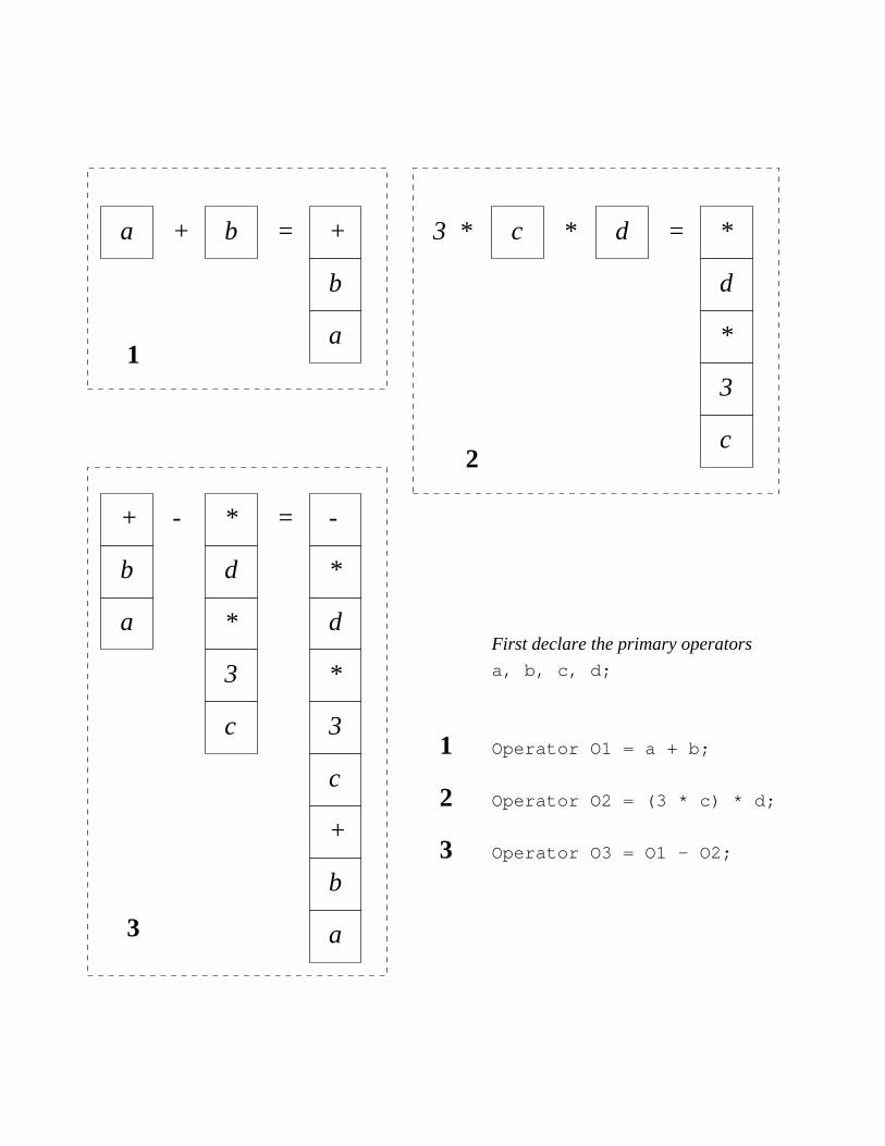
The program represents composite operators, i.e., sums and products of primary oper-ators, by stacks containing pointers to primary operators as illustrated in Fig. 1. Thosestacks are the principal member data of the Operator class, which is the parent class ofPrimaryOperator and therefore of all special classes derived from PrimaryOperator. Fora primary operator like SigmaPlus, the stack consists just of the pointer to *this, whichpoints to the primary operator itself. Figure 2 shows the hierarchy of operator classes.

The example stack in box 3 in Fig. 1 is generated by the code segment

Operator O1 = a + b;

Operator O2 = (3 * c) * d;

Operator O3 = 01 - 02;

where a, b, c, d are assumed to be primary operators defined earlier in the program.The example illustrates how addition, subtraction, and multiplication of Operators isimplemented in terms of operations on the stack. Further operations defined for Operatorsinclude Hermitian conjugation and raising to an integer power. The C++ inheritancemechanism ensures that all these operations are also defined for the derived primary-operator classes like SigmaPlus.

To apply an Operator to a State, the ‘*’ operator can be used as in the followingexample, where psi is a State and O3 is defined above:

State psi1 = O3 * psi;

Internally, this is implemented as a recursive evaluation of the stack. The order in whichthe primary operators are applied in the example can be inferred from the parentheses in

O3|ψ〉 =(

a + b− 3cd)

|ψ〉 =(

a|ψ〉 + b|ψ〉)

− c(

3(d|ψ〉))

. (13)

The program keeps the number of operations and the number of temporary States itcreates to a minimum. Some care has to be exercised, however, to avoid an inefficientevaluation order. E.g., in the code segment

double x=1.5;

SigmaPlus Sp;

State psi1 = 2.0*x*Sp*psi;

the state Sp*psi is first multiplied by 1.5, then by 2.0, whereas in

double x=1.5;

SigmaPlus Sp;

State psi1 = (2.0*x)*Sp*psi;

9

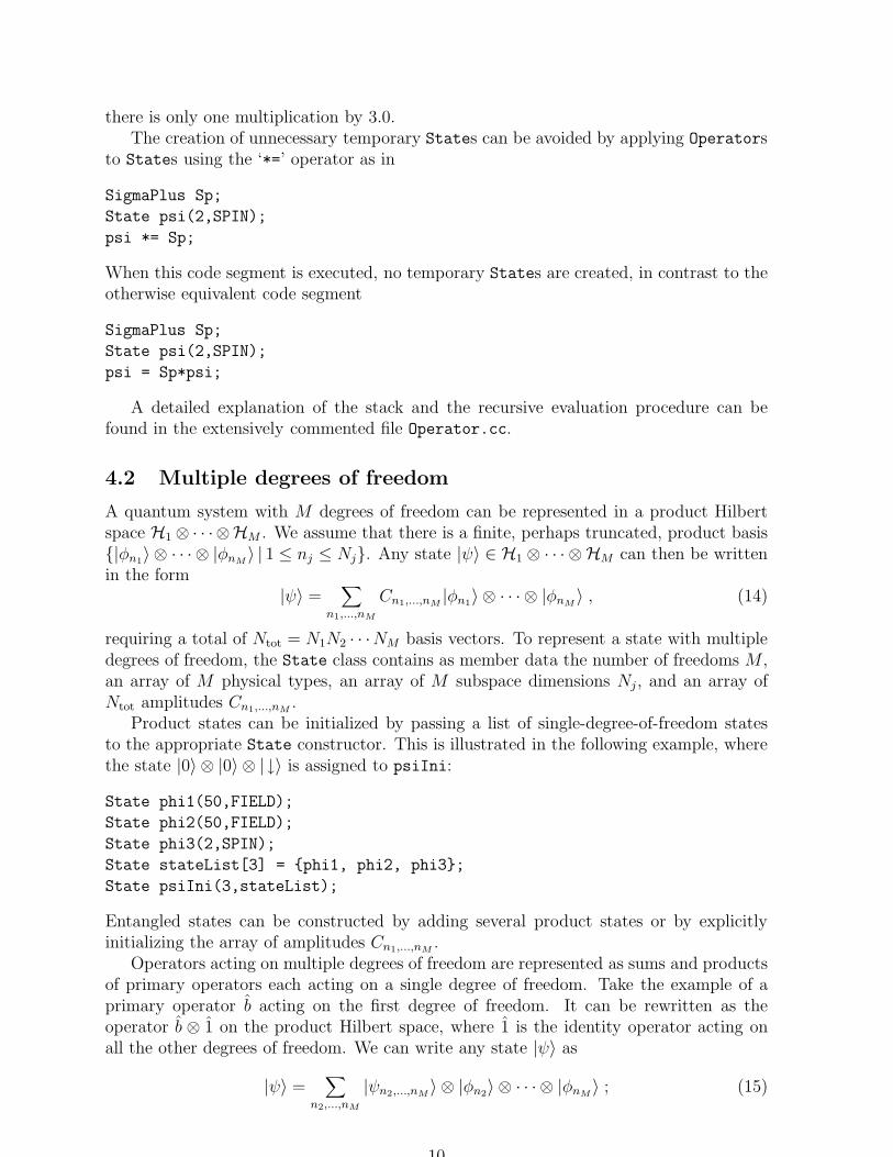
there is only one multiplication by 3.0.The creation of unnecessary temporary States can be avoided by applying Operators

to States using the ‘*=’ operator as in

SigmaPlus Sp;

State psi(2,SPIN);

psi *= Sp;

When this code segment is executed, no temporary States are created, in contrast to theotherwise equivalent code segment

SigmaPlus Sp;

State psi(2,SPIN);

psi = Sp*psi;

A detailed explanation of the stack and the recursive evaluation procedure can befound in the extensively commented file Operator.cc.

4.2 Multiple degrees of freedom

A quantum system with M degrees of freedom can be represented in a product Hilbertspace H1 ⊗ · · · ⊗HM . We assume that there is a finite, perhaps truncated, product basis{|φn1〉 ⊗ · · · ⊗ |φnM

〉 | 1 ≤ nj ≤ Nj}. Any state |ψ〉 ∈ H1 ⊗ · · · ⊗ HM can then be writtenin the form

|ψ〉 =∑

n1,...,nM

Cn1,...,nM|φn1〉 ⊗ · · · ⊗ |φnM

〉 , (14)

requiring a total of Ntot = N1N2 · · ·NM basis vectors. To represent a state with multipledegrees of freedom, the State class contains as member data the number of freedoms M ,an array of M physical types, an array of M subspace dimensions Nj , and an array ofNtot amplitudes Cn1,...,nM

.Product states can be initialized by passing a list of single-degree-of-freedom states

to the appropriate State constructor. This is illustrated in the following example, wherethe state |0〉 ⊗ |0〉 ⊗ |↓〉 is assigned to psiIni:

State phi1(50,FIELD);

State phi2(50,FIELD);

State phi3(2,SPIN);

State stateList[3] = {phi1, phi2, phi3};

State psiIni(3,stateList);

Entangled states can be constructed by adding several product states or by explicitlyinitializing the array of amplitudes Cn1,...,nM

.Operators acting on multiple degrees of freedom are represented as sums and products

of primary operators each acting on a single degree of freedom. Take the example of aprimary operator b acting on the first degree of freedom. It can be rewritten as theoperator b ⊗ 1 on the product Hilbert space, where 1 is the identity operator acting onall the other degrees of freedom. We can write any state |ψ〉 as

|ψ〉 =∑

n2,...,nM

|ψn2,...,nM〉 ⊗ |φn2〉 ⊗ · · · ⊗ |φnM

〉 ; (15)

10

the action of b⊗ 1 on |ψ〉 is therefore given by the action of b on the first degree of freedominside a hierarchy of loops over all the other degrees of freedom:

(

b⊗ 1)

|ψ〉 =∑

n2,...,nM

(

b|ψn2,...,nM〉)

⊗ |φn2〉 ⊗ · · · ⊗ |φnM〉 . (16)

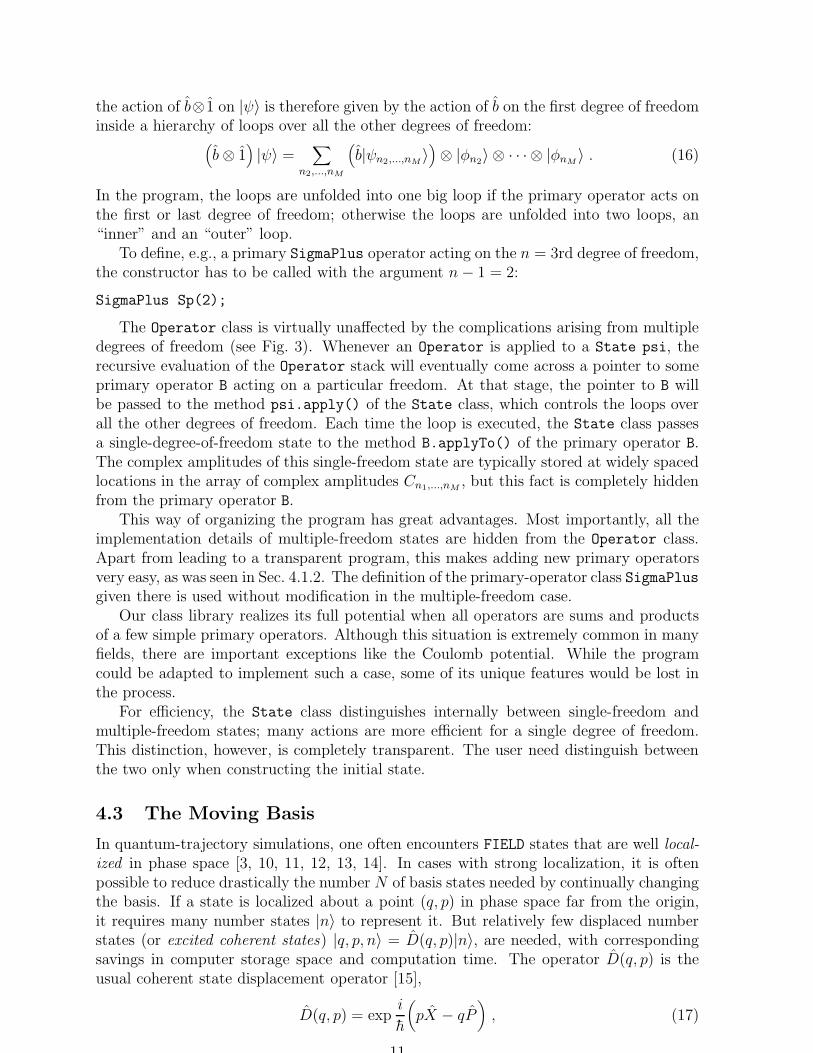
In the program, the loops are unfolded into one big loop if the primary operator acts onthe first or last degree of freedom; otherwise the loops are unfolded into two loops, an“inner” and an “outer” loop.

To define, e.g., a primary SigmaPlus operator acting on the n = 3rd degree of freedom,the constructor has to be called with the argument n− 1 = 2:

SigmaPlus Sp(2);

The Operator class is virtually unaffected by the complications arising from multipledegrees of freedom (see Fig. 3). Whenever an Operator is applied to a State psi, therecursive evaluation of the Operator stack will eventually come across a pointer to someprimary operator B acting on a particular freedom. At that stage, the pointer to B willbe passed to the method psi.apply() of the State class, which controls the loops overall the other degrees of freedom. Each time the loop is executed, the State class passesa single-degree-of-freedom state to the method B.applyTo() of the primary operator B.The complex amplitudes of this single-freedom state are typically stored at widely spacedlocations in the array of complex amplitudes Cn1,...,nM

, but this fact is completely hiddenfrom the primary operator B.

This way of organizing the program has great advantages. Most importantly, all theimplementation details of multiple-freedom states are hidden from the Operator class.Apart from leading to a transparent program, this makes adding new primary operatorsvery easy, as was seen in Sec. 4.1.2. The definition of the primary-operator class SigmaPlusgiven there is used without modification in the multiple-freedom case.

Our class library realizes its full potential when all operators are sums and productsof a few simple primary operators. Although this situation is extremely common in manyfields, there are important exceptions like the Coulomb potential. While the programcould be adapted to implement such a case, some of its unique features would be lost inthe process.

For efficiency, the State class distinguishes internally between single-freedom andmultiple-freedom states; many actions are more efficient for a single degree of freedom.This distinction, however, is completely transparent. The user need distinguish betweenthe two only when constructing the initial state.

4.3 The Moving Basis

In quantum-trajectory simulations, one often encounters FIELD states that are well local-

ized in phase space [3, 10, 11, 12, 13, 14]. In cases with strong localization, it is oftenpossible to reduce drastically the number N of basis states needed by continually changingthe basis. If a state is localized about a point (q, p) in phase space far from the origin,it requires many number states |n〉 to represent it. But relatively few displaced numberstates (or excited coherent states) |q, p, n〉 = D(q, p)|n〉, are needed, with correspondingsavings in computer storage space and computation time. The operator D(q, p) is theusual coherent state displacement operator [15],

D(q, p) = expi

h

(

pX − qP)

, (17)

11

where X and P are the position and momentum operators. The separation of the rep-resentation into a classical part (q, p) and a quantum part |q, p, n〉 is called the moving

basis [16] or, as in [13], the mixed representation. To represent a state of type FIELD inthe moving basis requires to store the complex center of coordinates α = (q + ip)/

√2 in

addition to the complex amplitudes. A multiple-freedom state in the moving basis withseveral freedoms of type FIELD requires an array of centers of coordinates.

Implementing the moving basis algorithm is straightforward. Suppose that at timet = t0 the state |ψ(t0)〉 is represented in the basis |q0, p0, n〉, centered at

(q0, p0) = (〈ψ(t0)|X|ψ(t0)〉, 〈ψ(t0)|P |ψ(t0)〉). (18)

Then after one discrete time step, the expectations in this basis shift to

(q1, p1) = (〈ψ(t0 + δt)|X|ψ(t0 + δt)〉, 〈ψ(t0 + δt)|P |ψ(t0 + δt)〉) 6= (q0, p0). (19)

The computational advantage of a small number of basis states is then retained by chang-ing the representation to the shifted basis |q1, p1, n〉 centered at q1 and p1. This shift inthe origin of the basis represents the elementary single step of the moving basis.

The components of |ψ(t0 + δt)〉 can be computed using the expressions given above.The computing time needed for the basis shift is of the same order of magnitude asfor computing a single discrete time step of one of the quantum trajectory equations.Shifting the basis once every discrete time step could therefore double the computingtime, depending on the complexity of the Hamiltonian and the number of degrees offreedom. On the other hand, the reduced number of basis vectors needed to representstates in the moving basis can lead to savings far bigger than a factor of 2.

In the example of second harmonic generation discussed in [16], two modes of theelectromagnetic field interact. Using the moving basis reduces the number of basis vectorsneeded by a factor of 100 in each mode. The total number of basis vectors needed is thusreduced by a factor of 10000, leading to reduction in computing time by a factor of roughly10000/2 = 5000. Furthermore, the fixed basis would exceed the memory capacity of mostcomputers.

The State class includes a variety of basis-changing methods. The most important isthe method

void moveCoords( const Complex& displacement, int theFreedom,

double shiftAccuracy );

which performs a relative shift of the center of coordinates α = (q+ ip)/√

2 by an amountgiven by the complex argument displacement. The integer argument theFreedom spec-ifies which degree of freedom is to be shifted—this degree of freedom must be of typeFIELD. The double argument shiftAccuracy gives the numerical accuracy with whichto make the shift. The physical state is unchanged by applying moveCoords(), but itis represented in a new basis. The method moveCoords() is used in the stochastic inte-gration algorithms of the Trajectory class described in Sec. 5. The primary operatorsof type FIELD defined in the files FieldOp.h and FieldOp.cc are implemented in such away that they can handle moving-basis states as well as ordinary states.

The quantum trajectory equations can contain both localizing and delocalizing terms.[3, 10, 11, 12, 13, 14]. Nonlinear terms in the Hamiltonian tend to spread the wave functionin phase space, whereas the Lindblad terms often cause it to localize. Accordingly, thewidth of the wave packets varies along a typical trajectory. We use this to reduce the

12

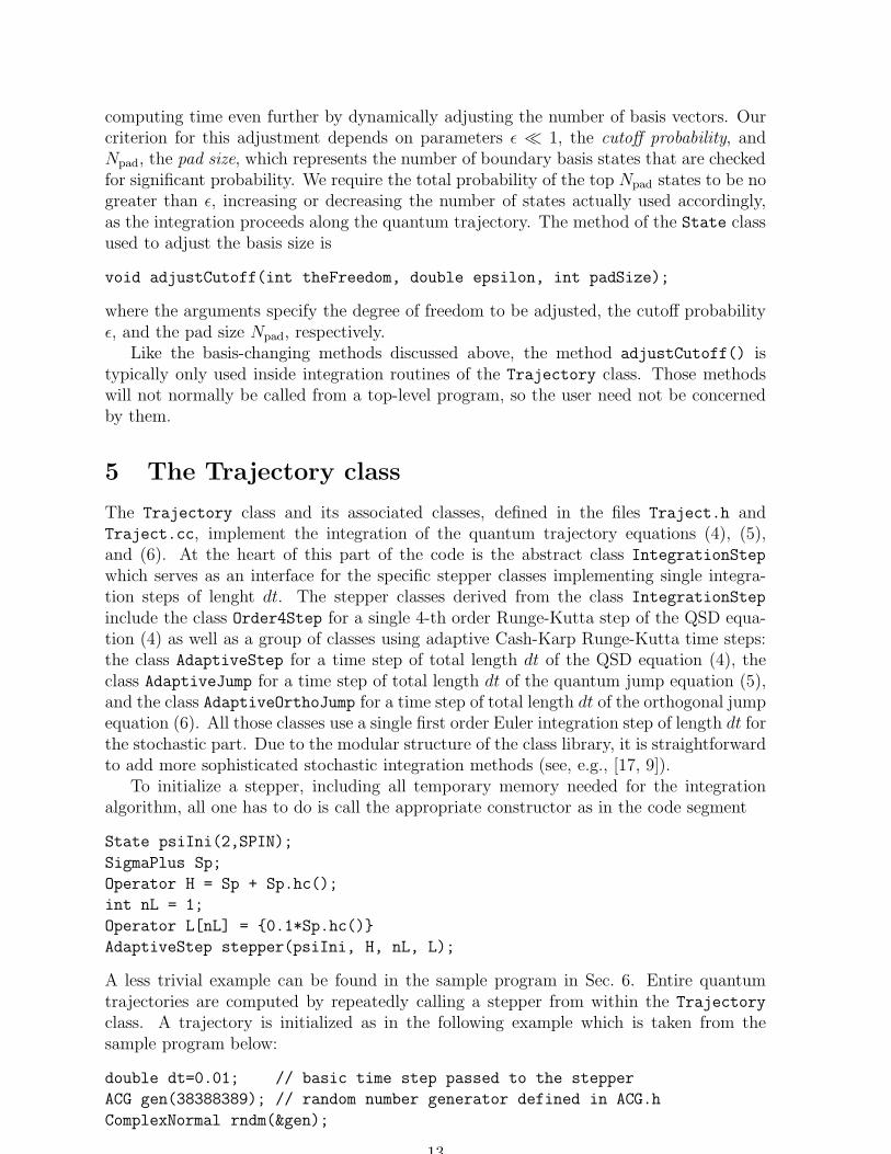
computing time even further by dynamically adjusting the number of basis vectors. Ourcriterion for this adjustment depends on parameters ǫ ≪ 1, the cutoff probability, andNpad, the pad size, which represents the number of boundary basis states that are checkedfor significant probability. We require the total probability of the top Npad states to be nogreater than ǫ, increasing or decreasing the number of states actually used accordingly,as the integration proceeds along the quantum trajectory. The method of the State classused to adjust the basis size is

void adjustCutoff(int theFreedom, double epsilon, int padSize);

where the arguments specify the degree of freedom to be adjusted, the cutoff probabilityǫ, and the pad size Npad, respectively.

Like the basis-changing methods discussed above, the method adjustCutoff() istypically only used inside integration routines of the Trajectory class. Those methodswill not normally be called from a top-level program, so the user need not be concernedby them.

5 The Trajectory class

The Trajectory class and its associated classes, defined in the files Traject.h andTraject.cc, implement the integration of the quantum trajectory equations (4), (5),and (6). At the heart of this part of the code is the abstract class IntegrationStep

which serves as an interface for the specific stepper classes implementing single integra-tion steps of lenght dt. The stepper classes derived from the class IntegrationStep

include the class Order4Step for a single 4-th order Runge-Kutta step of the QSD equa-tion (4) as well as a group of classes using adaptive Cash-Karp Runge-Kutta time steps:the class AdaptiveStep for a time step of total length dt of the QSD equation (4), theclass AdaptiveJump for a time step of total length dt of the quantum jump equation (5),and the class AdaptiveOrthoJump for a time step of total length dt of the orthogonal jumpequation (6). All those classes use a single first order Euler integration step of length dt forthe stochastic part. Due to the modular structure of the class library, it is straightforwardto add more sophisticated stochastic integration methods (see, e.g., [17, 9]).

To initialize a stepper, including all temporary memory needed for the integrationalgorithm, all one has to do is call the appropriate constructor as in the code segment

State psiIni(2,SPIN);

SigmaPlus Sp;

Operator H = Sp + Sp.hc();

int nL = 1;

Operator L[nL] = {0.1*Sp.hc()}

AdaptiveStep stepper(psiIni, H, nL, L);

A less trivial example can be found in the sample program in Sec. 6. Entire quantumtrajectories are computed by repeatedly calling a stepper from within the Trajectory

class. A trajectory is initialized as in the following example which is taken from thesample program below:

double dt=0.01; // basic time step passed to the stepper

ACG gen(38388389); // random number generator defined in ACG.h

ComplexNormal rndm(&gen);

13

// Gaussian random numbers defined in CmplxRan.h

Trajectory traj(psiIni, dt, stepper, &rndm);

The Trajectory class comprises two methods to launch the simulation, compute ex-pectation values of operators of interest, and produce output. The use of the methodplotExp(), designed to simulate a single trajectory, is explained in Sec. 6. The methodsumExp(), which is very similar to plotExp(), can be used to compute the mean expec-tation values of operators averaged over many trajectories.

6 Sample program and template

In this section, we illustrate the main features of the class library in a complete exampleprogram which can be used as a template. The example program computes expectationvalues for a single trajectory of the quantum state diffusion equation (4); to computemeans over many trajectories, one simply replaces the call to traj.plotExp() in thetemplate by a call to traj.sumExp(). The system has three degrees of freedom: twononlinearly coupled field modes described by annihilation operators a1 and a2, and aspin described by raising and lowering operators σ+ and σ−. The Hamiltonian in theinteraction picture is [18]

H = Ei(a†1 − a1) +χ

2i(a†21 a2 − a2

1a†2) + ωσ+σ− + ηi(a2σ+ − a†2σ−) , (20)

where E is the strength of an external pump field, χ is the strength of the nonlinearinteraction, ω is the detuning between the frequency of the field mode a2 and the spintransition frequency, and η is the strength of the coupling of the spin to the field modea2. The Lindblad operators

L1 =√

2γ1 a1 , L2 =√

2γ2 a2 , L3 =√

2κ σ− (21)

describe dissipation of the field modes and the spin with coefficients γ1, γ2, and κ, respec-tively.

The trajectory’s initial state is the product state |ψini〉 = |0〉⊗|0〉⊗|↓〉. The integrationstep-size is dt=0.01 and the total integration time is 500*dt = 5. The integration stepperAdaptiveStep implements a single time step of length dt of the QSD equation (4) usingthe Cash-Karp Runge-Kutta algorithm with adaptive time steps [8] for the deterministicpart and first-order Euler integration for the stochastic part.

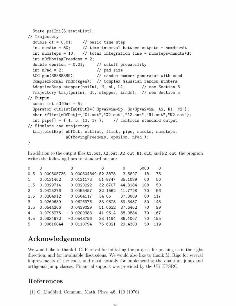
At times that are integer multiples of 50*dt = 0.5, the expectation values of theoperators specified in the array outlist are computed and written to the files specified inthe array flist. E.g., the first element of outlist is the operator X1 ≡ σ+a2σ−σ+. Attimes t = 0, 0.5, . . . , 5.0, the method plotExp computes the expectation values 〈X1〉 andvar(X1) ≡ 〈X1 − 〈X1〉〉 and writes t, Re(〈X1〉), Im(〈X1〉), Re(var(X1)), and Im(var(X1))to the file X1.out. In addition, each time a set of expectation values is computed, theprogram writes 7 numbers to standard output (see the sample output below): the timet, 4 expectation values determined by the integer array pipe, the number of basis statesused, and the number of adaptive steps taken. The integers in the array pipe correspondto the columns in the output files containing expectation values (i.e., columns 2 through5 of each output file). In the present example, expectation values are computed for the 5operators σ+a2σ−σ+, σ−σ+a2σ−, a2, n1, and n2, which are written to 5 output files withnumbered columns 1 through 20. According to the expression int pipe[]={1,5,13,17},

14

the expectation values written to standard output are Re(〈σ+a2σ−σ+〉), Re(〈σ−σ+a2σ−〉),Re(〈n1〉), and Re(〈n2〉).

The moving basis is used for both FIELD degrees of freedom. The basis size is dynam-ically adjusted with a cutoff probability ǫ = 0.01 and a pad size Npad = 2. The sampleoutput below shows how the basis size changes with time. Initially, 5000 = 50 ∗ 50 ∗ 2states are allocated, but at time t = 0.5, only 18 states are needed. Subsequently, thebasis size fluctuates around a typical size of 70 states.

Here is the complete program:

#include "Complex.h"

#include "ACG.h"

#include "CmplxRan.h"

#include "State.h"

#include "Operator.h"

#include "FieldOp.h"

#include "SpinOp.h"

#include "Traject.h"

int main()

{

// Primary Operators

AnnihilationOperator A1(0); // 1st freedom

NumberOperator N1(0);

AnnihilationOperator A2(1); // 2nd freedom

NumberOperator N2(1);

SigmaPlus Sp(2); // 3rd freedom

Operator Sm = Sp.hc(); // Hermitian conjugate

Operator Ac1 = A1.hc();

Operator Ac2 = A2.hc();

// Hamiltonian

double E = 20.0;

double chi = 0.4;

double omega = -0.7;

double eta = 0.001;

Complex I(0.0,1.0);

Operator H = (E*I)*(Ac1-A1)

+ (0.5*chi*I)*(Ac1*Ac1*A2 - A1*A1*Ac2)

+ omega*Sp*Sm + (eta*I)*(A2*Sp-Ac2*Sm);

// Lindblad operators

double gamma1 = 1.0;

double gamma2 = 1.0;

double kappa = 0.1;

const int nL = 3;

Operator L[nL]={sqrt(2*gamma1)*A1,sqrt(2*gamma2)*A2,sqrt(2*kappa)*Sm};

// Initial state

State phi1(50,FIELD); // see Section 4.2

State phi2(50,FIELD);

State phi3(2,SPIN);

State stateList[3] = {phi1,phi2,phi3};

15

State psiIni(3,stateList);

// Trajectory

double dt = 0.01; // basic time step

int numdts = 50; // time interval between outputs = numdts*dt

int numsteps = 10; // total integration time = numsteps*numdts*dt

int nOfMovingFreedoms = 2;

double epsilon = 0.01; // cutoff probability

int nPad = 2; // pad size

ACG gen(38388389); // random number generator with seed

ComplexNormal rndm(&gen); // Complex Gaussian random numbers

AdaptiveStep stepper(psiIni, H, nL, L); // see Section 5

Trajectory traj(psiIni, dt, stepper, &rndm); // see Section 5

// Output

const int nOfOut = 5;

Operator outlist[nOfOut]={ Sp*A2*Sm*Sp, Sm*Sp*A2*Sm, A2, N1, N2 };

char *flist[nOfOut]={"X1.out","X2.out","A2.out","N1.out","N2.out"};

int pipe[] = { 1, 5, 13, 17 }; // controls standard output

// Simulate one trajectory

traj.plotExp( nOfOut, outlist, flist, pipe, numdts, numsteps,

nOfMovingFreedoms, epsilon, nPad );

}

In addition to the output files X1.out, X2.out, A2.out, N1.out, and N2.out, the programwrites the following lines to standard output:

0 0 0 0 0 5000 0

0.5 0.000505736 0.000504849 52.3875 3.5807 18 75

1 0.0131402 0.0131173 51.8747 35.1089 60 50

1.5 0.0329714 0.0320222 32.8707 44.3184 108 50

2 0.0425276 0.0455457 32.1562 41.7798 70 56

2.5 0.0284912 0.0564117 34.85 37.8809 80 117

3 0.0260639 0.0626976 33.9828 39.3437 80 143

3.5 0.0544306 0.0439029 51.0632 37.6462 70 99

4 0.0796275 -0.0209383 41.9614 38.0884 70 167

4.5 0.0834672 -0.0543796 33.1194 36.1007 70 195

5 -0.00616844 0.0110794 76.6321 29.4303 50 119

Acknowledgements

We would like to thank I. C. Percival for initiating the project, for pushing us in the rightdirection, and for invaluable discussions. We would also like to thank M. Rigo for severalimprovements of the code, and most notably for implementing the quantum jump andorthgonal jump classes. Financial support was provided by the UK EPSRC.

References

[1] G. Lindblad, Commun. Math. Phys. 48, 119 (1976).

16

[2] L. Diosi, Phys. Lett. A 114, 451 (1986).

[3] N. Gisin and I. C. Percival, J. Phys. A 25, 5677 (1992).

[4] H. J. Carmichael, An Open Systems Approach to Quantum Optics (Springer, Berlin,1993).

[5] J. Dalibard, Y. Castin, and K. Mølmer, Phys. Rev. Lett. 68, 580 (1992).

[6] C. W. Gardiner, A. S. Parkins, and P. Zoller, Phys. Rev. A 46, 4363 (1992).

[7] J. K. Breslin, G. J. Milburn, and H. M. Wiseman, Phys. Rev. Lett. 74, 4827 (1995).

[8] W. H. Press, S. A. Teukolsky, W. T. Vetterling, and B. P. Flannery, Numerical

Recipes in C, 2nd ed. (Cambridge University Press, Cambridge, 1992).

[9] J. Steinbach, B. M. Garraway, and P. L. Knight, Phys. Rev. A 51, 3302 (1995).

[10] L. Diosi, Phys. Lett. A 132, 233 (1988).

[11] N. Gisin and I. C. Percival, J. Phys. A 26, 2245 (1993).

[12] I. C. Percival, J. Phys. A 27, 1003 (1994).

[13] T. Steimle, G. Alber, and I. C. Percival, J. Phys. A 28, L491 (1995).

[14] M. Holland, S. Marksteiner, P. Marte, and P. Zoller, Phys. Rev. Lett. 76, 3683 (1996).

[15] W. H. Louisell, Quantum Statistical Properties of Radiation (Wiley, New York, 1973).

[16] R. Schack, T. A. Brun, and I. C. Percival, J. Phys. A 28, 5401 (1995).

[17] P. E. Kloeden and E. Platen, Numerical Solution of Stochastic Differential Equations

(Springer, Berlin, 1992).

[18] R. Schack, T. A. Brun, and I. C. Percival, Phys. Rev. A 53, 2694 (1996).

17

Figure 1: These examples show how the internal stack representations of primary andcomposite Operators are combined in arithmetic operations. Notice that while arithmeticexpressions are parsed from left to right, the order in which Operators are applied toStates is from right to left.

Figure 2: In this diagram, the arrows point from parent classes to derived classes. Theclasses listed in each box are declared in the #include file given above the box. Arithmeticoperations are defined in the Operator class. The PrimaryOperator class serves as aninterface for the specific FIELD, SPIN, and ATOM operators. Adding operators of either anexisting or a new type is straightforward.

Figure 3: When a pointer to a primary operator acting on a particular freedom is encoun-tered during the evaluation of an Operator stack, control is passed to the State class,where within loops over the basis states of all the other degrees of freedom, the primaryoperator is applied to a succession of single-freedom states. This means that the Operatorclass and its derived classes do not need to distinguish between single and multiple free-dom states; all details concerning the multiple-freedom case are hidden within the State

class.

18

a b c d+ = 3 * * =

- = -

1

2

3

Operator O3 = O1 - O2;

Operator O1 = a + b;

First declare the primary operators

a, b, c, d;

1

2

3

+ *

*a

b

*+

d

3

c

b

a

d

*

3

c

*

d

*

3

c

+

b

Operator O2 = (3 * c) * d;

a

=, +, -, *, +=, -=, *=

hc(), pow()

applyTo()

PrimOp.h

FieldOp.h SpinOp.h

Operator

PrimaryOperator

AnnihilationOperator

NumberOperator

IdentityOperator

XOperator

POperator

SigmaX

SigmaY

SigmaZ

SigmaPlus

TransitionOperator

AtomOp.h

Operator.h

a = (x+ ip)=p2n = aya1p = i(ay � a)=p2x = (a+ ay)=p2 jiihjj�x�y�z�+

Operator

PrimaryOperator

applyTo()

apply()

Apply each primary operator to the state;

tranformed state returned.

Loop over all other degrees of freedom.

Pass succession of one-freedom states

to primary operator; transformed states

returned.

Act on single freedom states.

Stack points

act on particular

freedoms.

State

M degrees of freedom.

to primary

operators which