A CASE STUDY ON SUPPORT VECTOR MACHINES VERSUS

ARTIFICIAL NEURAL NETWORKS by

Wen-Chyi Lin

BS, Chung-Cheng Institute of Technology, 1998

Submitted to the Graduate Faculty of

School of Engineering in partial fulfillment

of the requirements for the degree of

Master of Science

University of Pittsburgh

2004

ii

UNIVERSITY OF PITTSBURGH

SCHOOL OF ENGINEERING

This thesis was presented

by

Wen-Chyi Lin

It was defended on

July 21, 2004

and approved by

J. Robert Boston, Professor, Department of Electrical Engineering

Luis F. Chaparro, Associate Professor, Department of Electrical Engineering

Thesis Advisor: Ching-Chung Li, Professor, Department of Electrical Engineering

iii

ABSTRACT

A CASE STUDY ON SUPPORT VECTOR MACHINES VERSUS ARTIFICIAL NEURAL NETWORKS

Wen-Chyi Lin, MS

University of Pittsburgh, 2004

The capability of artificial neural networks for pattern recognition of real world problems is

well known. In recent years, the support vector machine has been advocated for its structure risk

minimization leading to tolerance margins of decision boundaries. Structures and performances of

these pattern classifiers depend on the feature dimension and training data size. The objective of

this research is to compare these pattern recognition systems based on a case study. The particular

case considered is on classification of hypertensive and normotensive right ventricle (RV) shapes

obtained from Magnetic Resonance Image (MRI) sequences. In this case, the feature dimension is

reasonable, but the available training data set is small, however, the decision surface is highly

nonlinear.

For diagnosis of congenital heart defects, especially those associated with pressure and

volume overload problems, a reliable pattern classifier for determining right ventricle function is

needed. RV’s global and regional surface to volume ratios are assessed from an individual’s MRI

heart images. These are used as features for pattern classifiers. We considered first two linear

classification methods: the Fisher linear discriminant and the linear classifier trained by the

Ho-Kayshap algorithm. When the data are not linearly separable, artificial neural networks with

back-propagation training and radial basis function networks were then considered, providing

iv

nonlinear decision surfaces. Thirdly, a support vector machine was trained which gives tolerance

margins on both sides of the decision surface. We have found in this case study that the

back-propagation training of an artificial neural network depends heavily on the selection of initial

weights, even though randomized. The support vector machine where radial basis function kernels

are used is easily trained and provides decision tolerance margins, in spite of only small margins.

v

TABLE OF CONTENTS 1.0 INTRODUCTION………………………………………………………….……………….… 1

1.1 BACKGROUND AND MOTIVATION….……...….………………………………….. 1

1.2 STATEMENT OF THE PROBLEM…………………..…………………………….......4

1.3 OUTLINE………………………………………………...….………………….………....5

2.0 LINEAR DISCRIMINANT FUNCTIONS……………………..…………………..…..………6

2.1 INTRODUCTION…………………………………………………..………………......6

2.2 FISHER LINEAR DISCRIMINANTS..……………………………………………..……7

2.3 THE HO-KASHYAP TRAINING ALGORITHM……………………………….………11

2.4 SUMMARY…………………………………………………………………………….14

3.0 ARTIFICIAL NEURAL NETWORKS AND RADIAL BASIS FUNCTIONS…………….…15

3.1 ARTIFICIAL NEURAL NETWORKS………………………………………………….15

3.1.1 Back-Propagation Training….…………….…………………….………………...19

3.1.2 ANN Trained for Right Ventricle Shape Data……….……...…….....................…21

3.1.3 Jackknife Training and Error Estimation…....……………………………….....…24

3.2 RADIAL BASIS FUNCTION NETWORKS……………………..…….….……..…32

3.2.1 Training………………..………………………………….………………………35

3.2.2 RBF Jackknife Error Estimation………………………………………….…….…37

3.3 SUMMARY OF RESULTS………………………………………………….………...…38

4.0 SUPPORT VECTOR MACHINES………………………….………………………..………39

4.1 LINEAR SUPPORT VECTOR MACHINES………….………….…………………….39

4.1.1 Leave-One-Out Bound…………………………..………….…………………….42

4.1.2 Training a SVM………………………………….………….……………..……..43

4.2 LINEAR SOFT MARGIN CLASSIFIER FOR OVERLAPPING PATTERNS ….……44

vi

4.3 NONLINEAR SUPPORT VECTOR MACHINES……………………….……………..45

4.3.1 Inner-Product Kernel……………………………….……….……………………46

4.3.2 Construction of a SVM…………………………….………………….…………49

4.4 SUPPORT VECTOR MACHINES FOR RIGHT VENTRICLE SHAPE CLASSIFICATION……………………………………………………………………51

5.0 CONCLUSIONS AND FUTURE WORK…………………..………….…...…………..….58

APPENDIX A……………………………………………………………………….…………...60

APPENDIX B..…………………………………………………………………..………..…61

BIBLIOGRAPHY..……………………………………………….…....…..……..……………..…62

vii

LIST OF TABLES Table 2-1 Fisher’s Linear Discriminant Analysis Result of 5-Feature RV Shape Data……………11

Table 2-2 Results of the Ho-Kashyap Training Procedure.………………………………....…..12

Table 2-3 Weights, Bias and Errors of the Ho-Kayshap Training Procedure…………………….13 Table 3-1: Table 3-1 Initial Weights of the ANN Trained without Momentum by 23 RV

Shape Samples………………………………………………………………………………22

Table 3-2 Final Weights of the ANN Trained without Momentum by 23 RV Shape Samples.…...22

Table 3-3 Initial Weights of the ANN Trained with Momentum by 23 RV Shape Samples.………23

Table 3-4 Final Weights of the ANN Trained with Momentum by 23 RV Shape Samples.….…....24

Table 3-5 14 Training Subsets (Normal: 7 HTN: 7) and Trained Results at 30 epochs…..….……25

Table 3-6 Jackknife Training and Error Estimates (with Momentum).……………………..…..…26 Table 3-7 False Positive and Negative Rates of Jackknife Training and Error Estimates of the

ANN classification of RV Shape Data (using Learngdm in training)………………………26

Table 3-8 Jackknife Training and Error Estimates (without Momentum)…….…………..…..…28

Table 3-9 False Positive and Negative Rates of Jackknife Training and Error Estimates of the ANN classification of RV Shape Data (using Learngd in training)…..…………...….…..…28

Table 3-10 “Optimal” Training Subset Derived from Two Jackknife Error Estimations..…...….29

Table 3-11 ANN Initial Weights Trained by 11 Optimal Sample………………………….…..…29

Table 3-12 ANN Final Weights Trained by 11 Optimal Sample……………..………….…..…30

Table 3-13 Final Weights of RBF network..…………………………………………..….…..…36

Table 3-14 False Positive and Negative Rates of RBF Jackknife Error Estimates…................…37

Table 4-1 Specifications of Inner-Product Kernels………………………………………….…..…48

Table 4-2 Results of SVM with Gaussian Kernels………………………………………….…..…52

Table 4-3 Result of Leave-One-Out Testing.….…………………………………………….…..…56

Table 4-4 Results of SVM with Sigmoid Kernels………………….……………………….…..…57

viii

Table A-1 Sample Right Ventricle Shape Data Obtained from MRI Sequences with 11 Normal and 12 Hypertensive (HTN) Cases. Five Features Consist of Global and Four Regional Surface/Volum Ratios.………………………………………………………………...…60

ix

LIST OF FIGURES Figure 1-1 The Optimal Decision Surface that Separates Training Data of Two Classes with

the Maximal Margin………………………………………………………………….…..….3

Figure 1-2 Division of RV into 4 Different Regions……………………………………………..…4

Figure 2-1 Fisher Linear Discriminants Analysis Result of 5-Feature of RV Shape Data……...…10

Figure 3-1 Block Diagram of an Artificial Neuron……………………………………………...…16

Figure 3-2 A Feedforward Multilayed Artificial Neural Network………………………...…..…...17

Figure 3-3 An Abbreviated Sketch of the (5-3-1) ANN Indicating 5 Inputs, 3 Hidden Units and 1 Output Neuron.………………………………………………………………………..17

Figure 3-4 Learning Curve (with momentum) of ANN Trained by 23 Samples.……….................23

Figure 3-5 Learning Curve (with momentum) of ANN Trained by 11 Optimal Data.…………….30

Figure 3-6 Two dimensional plot of “Optimal” Training Samples (Bold) Given in Table 3-10….31

Figure 3-7 Block Diagram of a RBF Network………………………………….………………….33

Figure 3-8 Learning curve of the RBF Network. …………………………………………..…….36

Figure 4-1 Two out of Many Separating Lines: Upper, a Less Acceptable One with a Small

Margin, And Below, a Good One with a Large Margin…………………………………….41

Figure 4-2 Nonlinear Mapping from the Input Space to a High-Dimensional Feature Space..46

Figure 4-3 Block Diagram of a Nonlinear SVM for Training…………………………………….50

Figure 4-4 Block Diagram of the Trained SVM………………………..………………………….53

Figure 4-5 Decision Boundary in x1-x2 (Global S/V, 0-25%S/V) Plane with the Projection of Sample Patterns. ………………………………………………………………………….54

)(•ϕ

x

ACKNOWLEDGMENTS

I would like to thank my advisor, Professor C. C. Li for his guidance and encouragement

during this thesis. Also I would like to thank Professor J. R. Boston and Professor L. F. Chaparro,

my committee members, for their helpful reviews and comments, Dr. M. Kaygusuz (Pediatric

Cardiology, U. of Miami), Dr. R. Munoz and Dr. G. J. Boyle (Pediatric Cardiology, UPMC) for

their suggestions and for providing their experimental data used in this thesis. Finally, let me

give my gratitude to Ji-Ning Corporation, Taiwan, R.O.C for giving me a fellowship for my

graduate study.

1

1.0 INTRODUCTION

1.1 BACKGROUND AND MOTIVATION

The capability of artificial neural networks for pattern recognition of real world problems

is well known. With the increasing performance of modern computers and the urgent demand for

classifiers accuracy, recently the support vector machine has been advocated for its structure risk

minimization which gives tolerance margins of decision boundaries [1]. To compare these

pattern recognition systems, a classification problem of hypertensive and normotensive right

ventricle (RV) shapes obtained from Magnetic Resonance Image (MRI) sequences is considered

[2].

Discovery and understanding of the structures in data is crucial in constructing classifiers.

The separability of classes is a fundamental geometrical property and, therefore, attempting to

derive linear discriminants is a useful first step in the exploration. We considered first two linear

classification methods: the Fisher linear discriminant and the linear classifier trained by the

Ho-Kayshap algorithm.

Consider a two-class (ω1, ω2) problem, if the data samples {x} are linearly separable,

then there exists a weights vector w and a threshold b such that

y > 0, if x ∈ω1

, (1-1). y < 0, if x ∈ω2

bxy += tw

2

Fisher linear discriminant analysis [3] seeks directions of w that are most efficient for

discrimination. By calculating within-class scatter matrix SW, between-class scatter matrix SB,

and solving for a generalized eigenvalue problem, we will find the associated eigenvectors.

Projecting the data x onto the principal eigenvector, we can immediately tell from the results

whether the data are linearly separable or not. The Ho-Kashyap training algorithm [4] uses the

gradient descent procedure trying to find a weight vector w and a threshold b by minimizing the

criterion function

2=),( b-YwbwJ (1-2),

where

Y = (1-3),

and X1 and X2 are the training sample subsets of class 1 and class 2, respectively. If the samples

are linearly separable, there exists a w and a b > 0 such that

0>= bYw (1-4).

A decision hyperplane is given by

wtx + b = 0 (1-5).

When the data is not linearly separable, artificial neural networks with hidden units may

be trained. Learning the nonlinear decision surface is the key power provided by artificial neural

networks. Feedforward multilayered artificial neural networks with sigmoidal nonlinearity in

artificial neurons are the most commonly used networks along with the back-propagation

training. Alternatively, radial basis functions are used in the hidden layer of the network.

2

1

XX

－1－

1

2

1

3

To find an “optimal” decision surface which separates patterns of two classes, a support

vector machine (SVM) provides us a powerful tool to achieve this task. Using the kernel

mapping technique, a SVM can be trained to minimize the structural risk and to separate either

linearly or nonlinearly separable data. It gives tolerance margins on both sides of the decision

surface. The support vectors are those transformed training patterns that are closest to the

separating surface (Figure 1-1).

These different types of pattern classifiers have their separating characteristics and

different degrees of trainability depending on the nature of the problem, data dimensionality and

the available training data. This project undertakes a case study on classification of these pattern

classifiers.

Figure 1-1 The Optimal Decision Surface that Separates Training Data of Two Classes with the Maximal Margin.

×

x2

x1

Support vectors

× ×

× ×

×

× ○

○

○

○

○

○

○

Margin

Optimal Decision Surface

4

1.2 STATEMENT OF THE PROBLEM

The specific pattern classifier under consideration is a biomedical pattern recognition

problem. Consider that a 3 dimensional right ventricle is reconstructed from a cardiac MRI

sequence. The shape of the right ventricle contains the information pertaining to the normality or

the congenital heart defect. A quantitative classification of the RV shape has been suggested [2]

that utilizes measurement on surface-to-volume ratio. A RV is divided into four regions and each

is separated by 25% of the distance from the apex to the pulmonary valve as shown in Fig. 1-2.

The volume and surface area of each region are calculated to provide four regional

surface/volume (S/V) ratios, and the global surface/volume ratio of the whole RV is also

computed. They together provide five features to be used in pattern classification to detect

congenital heart defects, especially those associated with pressure and volume overload. Hence,

the hypertensive case is to be differential from the normotensive case, base on these five features.

II

III

IV

Figure 1-2 Division of RV into 4 Different Regions.

5

Training data are provided by Dr. Munoz and Dr. Kaygusuz, they were extracted from MRI

sequences of RV plastic casts. Their previous studies have shown that S/V ratio decreases in

general as RV becomes hypertensive. They trained an artificial neural network with two hidden

layers each having four neurons. Their result indicates that one of these patterns was incorrectly

classified. This is obviously a highly nonlinear separation problem.

In this thesis, we study the training of linear dicriminant functions, artificial neural

networks and SVMs, using these data as a case study. We hope to understand the RV data

structure, to reduce the number of the weights to be trained and to increase the classification

accuracy, in particular, to compare the performance of the trained feedforward artificial neural

network and that of the trained support vector machine.

1.3 OUTLINE

This thesis is composed of five chapters. The present chapter has introduced the

background and research objective for the case study on support vector machines versus artificial

neural networks. Chapter 2 deals with the problem of linear separability, both Fisher linear

discriminants analysis and the Ho-Kashyap training procedure are reviewed and experimented.

Chapter 3 discusses feedforward artificial neural networks as well as radial basis functions

network where sigmoidal and Gaussian functions are used respectively as nonlinear functions in

neural units. In each case, Jackknife training and error estimation are applied. Support vector

machines are trained with both sigmoidal and Gaussian kernel functions as discussed in Chapter

4. Experiment results are presented in each Chapter. In chapter 5, discussions and conclusions

are given, as well as the issues to be explored further.

6

2.0 LINEAR DISCRIMINANT FUNCTIONS

2.1 INTRODUCTION

The main goal of a classification problem is to find a classifier that can predict the label

of new unseen data correctly. In practice, the problem often begins with a finite training set

presumed to represent the expected input. Important information of the problem can be obtained

by learning from the training data. Separability of data is a fundamental geometrical property;

therefore, when we construct a classifier for linearly or nonlinearly separable data, it is useful to

explore linear discriminant functions as the first step.

Dimensionality of the data is one of the recurring problems we face when applying

statistical approaches to pattern recognition. Procedures that are analytically or computationally

accessible in low-dimensional spaces may become totally impractical in high-dimensions spaces.

The classical Fisher’s discriminant analysis is to examine separation of data in a high

dimensional space by projecting them into an appropriate line, the principal axis of the data.

In the next section, Fisher’s method is briefly reviewed. In Section 2.3, the Ho-Kashyap

training procedure is reviewed for the 2-class problem. If the sample patterns are linearly

separable, then any of the two methods will produce a linear classifier. However, if the sample

data are not linearly separable, then it indicates the nature of the possible non-linear separation of

the data. Section 2.4 gives a summary of the experimental results of these two methods when

applied to the RV shape data.

7

)(=~~1 21

T2 m-mw- mm

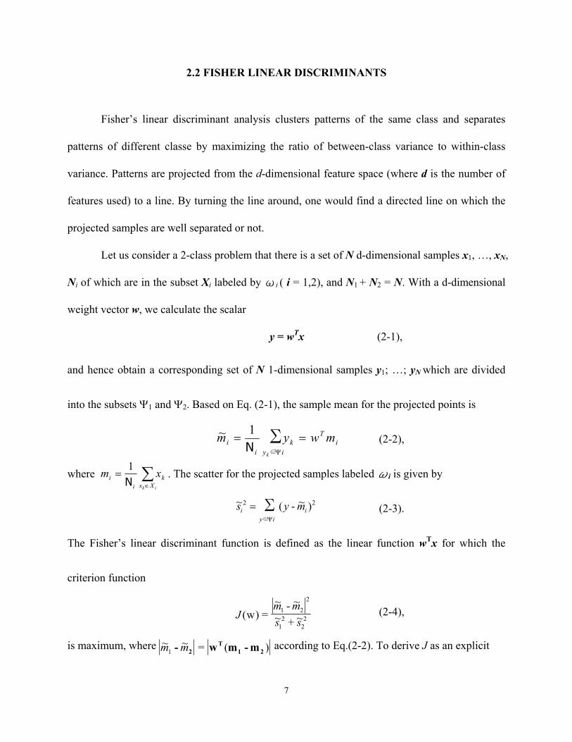
2.2 FISHER LINEAR DISCRIMINANTS

Fisher’s linear discriminant analysis clusters patterns of the same class and separates

patterns of different classe by maximizing the ratio of between-class variance to within-class

variance. Patterns are projected from the d-dimensional feature space (where d is the number of

features used) to a line. By turning the line around, one would find a directed line on which the

projected samples are well separated or not.

Let us consider a 2-class problem that there is a set of N d-dimensional samples x1, …, xN,

Ni of which are in the subset Xi labeled by ωi ( i = 1,2), and N1 + N2 = N. With a d-dimensional

weight vector w, we calculate the scalar

y = wTx (2-1),

and hence obtain a corresponding set of N 1-dimensional samples y1; …; yN which are divided

into the subsets Ψ1 and Ψ2. Based on Eq. (2-1), the sample mean for the projected points is

(2-2),

where . The scatter for the projected samples labeled ωi is given by

(2-3).

The Fisher’s linear discriminant function is defined as the linear function wTx for which the

criterion function

(2-4),

is maximum, where according to Eq.(2-2). To derive J as an explicit

∑∈

1~iy

iT

ki

ik

mwymΨ

==N

∑∈

=ik Xx

ki

i xmN1

2

∈

2 )~-(~ ∑ iiy

i mysΨ

=

22

21

2

21~+~

~-~=)(

ssmm

J w

8

function of w, we define the scatter matrices Si, the within-class scatter matrix SW and the

between-class scatter matrix SB as follows

(2-5),

SW = S1 + S2, (2-6),

and SB = (m1－m2)(m1－m2)T. (2-7).

Using Eq.(2-2), Eq.(2-3) and the definitions given above, we can obtain

22

21

~~ ss + = wT SWw (2-8),

and

2

21~~ mm - = wT SBw (2-9).

By substituting these expressions into Eq.(2-4), the criterion function J can be written as

J(w) = (2-10),

Maximizing J by taking 0w

=∂∂J leads to

Sww(wTSBw) = SBw(wTSww) (2-11).

Let λ= (wTSBw) (wTSww)-1 which is a scalar, then

λw = (Sw-1SB)w (2-12),

becomes an eigenvector problem. From Eq. (2-7), since

SBw = (m1－m2)(m1－m2)Tw = (m1－m2) k (2-13),

where k = (m1－m2)Tw is a scalar, SBw has the direction of (m1－m2),

T

Xxi

ik

S )m-x)(m-x( i∈

kik∑=

wwww

wT

BT

SS

9

λw = k Sw-1(m1－m2) (2-14).

The nonsingular SW gives the normalized solution of the weight vector w [7]

w = 1-wS (m1 － m2). (2-15).

Using the weight vector, all the sample patterns X’s are mapped onto a line y, forming two

subsets 1ϕ and 2ϕ with maximum interest distance and minimum intraset distance. To identify

a test pattern, compare the distance from the projected test pattern to each subsets iϕ , and the

test pattern is identified with the closest training subsets iϕ .

For the sample data set of right ventricle shapes given in Appendix A, which consist of

11 normal and 12 abnormal (hypertensive, HTN) patterns, five Surface/Volume features (global

S/V, 0-25%S/V, 25-50%S/V, 50%-75%S/V, and 75-100%S/V) form a 5-dimensional space.

Figure 2-1 and Table 2-1 show the Fisher linear discriminant analysis result where projection y

values are given. The computed weight vector, eigenvector, w is [0.1342 -0.0241 0.1931 0.9714

0.0230]T. Note that the two subsets are not completely separated, and pattern 1 (Normal-2) and

14 (HTN-12) cannot be correctly placed. In the next section, we will try to apply the

Ho-Kashyap algorithm to explore whether these two pattern classes can be linearly separated.

10

Figure 2-1 Fisher Linear Discriminant Analysis Result of 5-Feature of RV Shape Data.

A chosen reference

(－w0)

y

11

2.3 THE HO-KASHYAP TRAINING ALGORITHM

The Ho-Kashyap algorithm [4] combines the least mean squares errors and the gradient

descent procedures to train a weight vector w by minimizing the criterion function

2－=),( b YwbwJ (2-16),

where

Y = (2-17),

is the augmented pattern matrix, w is the augment weight vector with the threshold weight or

Normal HTN (abnormal) No. Projection y No. Projection y 1 5.0889 12 6.6827 2 7.3383 13 5.2614 3 9.9437 14 7.7649 4 8.2679 15 5.3735 5 8.4051 16 5.2193 6 7.0860 17 5.5820 7 8.5550 18 5.2666 8 8.7387 19 5.7094 9 7.9029 20 6.3509 10 8.9088 21 4.4162 11 7.2511 22 3.6836 23 5.9747

Table 2-1 Fisher’s Linear Discriminant Analysis Result of 5-Feature RV Shape Data.

2

1

XX

－1－

1

2

1

12

bias w0 as its first component, and b > 0. Let Y+ be the pseudo inverse of Y. The training

algorithm is stated as follows:

w(1) = Y+b(1), b(1) > 0 but otherwise arbitrary

e(k) = Yw(k)－b(k)

10),)()(()()1( <<++=+ ηη eebb kkkk

))()(()()1( kkkk eeYww ++=+ +η

This algorithm yields a solution vector w* for Yw* > 0 in finite number of steps, if the training

samples are linearly separable. If the training samples are not linearly separable, a non-positive

e(k) will occur in finite number if steps (components of e(k) are all non-positive with at least one

component to be negative); that indicates the nonlinear separability.

For the sample data set of right ventricle shapes given in Appendix A, and with η= 0.1

and b(1) given in Table 2-3, the algorithm terminates at iteration step 42 with an augmented

weight vector w = [ 0.1077 0.2980 0.2183 0.1615 0.1731 0.1800], and indicates that the sample

data are not linearly separable. Pattern No. 9 (Normal-13) and 22 (HTN-21) are incorrectly

placed as shown in Table 2-2.

Training Result by Applying the Ho-Kashyap procedure (Iterations:42)

Correct 1, 2, 3, 4, 5, 6, 7, 8, 10, 11, 12, 13, 14, 15, 16, 17, 18, 19, 20, 21, 23

Incorrect 9, 22

Table 2-2 Result of the Ho-Kashyap Training Procedure.

13

Initial w Final w No Initial b Final b Error e (1.0e-005 *)

0.5000 0.1077 1. 0.0158 5.6740 0.0000 0.5000 0.2980 2. 0.0164 7.6291 0.0000

0.5000 0.2183 3. 0.1901 12.4615 0.0000

0.5000 0.1615 4. 0.5869 9.9911 0.0000

0.5000 0.1731 5. 0.0576 9.0957 0.0000

0.5000 0.1800 6. 0.3676 9.3225 0.0000

Learning rate η 7. 0.6315 10.7204 0.0000

0.1 8. 0.7176 9.0691 0.0000

9. 0.6927 10.6469 -0.3839 10. 0.0841 12.2709 0.0000

11. 0.4544 9.1324 0.0000

12. 0.4418 7.5702 0.0000

13. 0.3533 6.2437 0.0000

14. 0.1536 8.8024 0.0000

15. 0.6756 6.2492 0.0000

16. 0.6992 6.8332 0.0000

17. 0.7275 7.0763 0.0000

18. 0.4784 6.5037 0.0000

19. 0.5548 6.1664 0.0000

20. 0.1210 7.1582 0.0000

21. 0.4508 6.3121 0.0000

22. 0.7159 3.6434 -0.6980

23. 0.8928 6.6628 0.0000

Table 2-3 Weights, Bias and Errors of the Ho-Kayshap Training Procedure.

14

2.4 SUMMARY

Both the Fisher’s linear discriminant analysis and the Ho-Kashyap training algorithm

indicate that the sample RV shape data are not linearly separable. Each experiment provides us

with a weight vector resulting in 2 classification errors of the training. One normal pattern falls

into the abnormal (HTN) region, and one HTN falls into the normal region. The condition of the

application of the Ho-Kayshap procedure clearly indicates the nonlinear separability of the data

which necessitates a nonlinear pattern classifier. We will study the use of artificial neural

networks and support vector machines on classifying right ventricle shape data.

15

3.0 ARTIFICIAL NEURAL NETWORKS AND RADIAL BASIS FUNCTIONS

n artificial neural network (ANN) is an information processing system that employs

certain characteristics of biological neural processors. It analyzes data by passing the data

through a number of neural units which are interconnected and highly distributed. A neural

network performs its processing by accepting inputs xi, which are then multiplied by a set of

weights wi. A neuron transforms the sum of the weighted inputs nonlinearly into an output value,

y, by using a nonlinear activation function or transfer function, T, as shown in Figure 3-1, where

T(s) is commonly represented by a sigmoidal function. A bias, w0, is added to the neuron, it is

then regarded as a weight, with a constant input of 1.

3.1 ARTIFICIAL NEURAL NETWORKS

We consider the feedforward multilayered perceptrons (MLPs), as shown in Figure 3-2,

that have been widely used in many applications. Hornik et al [5] proved that a three-layered

MLP with an unlimited number of neurons in the hidden layer can solve arbitrary nonlinear

mapping problems. However, the problem of training an MLP is NP-complete. As a result, we

often have a slow convergence problem when training an MLP. Moreover, the number of hidden

layers, neurons in a hidden layer, and connectivity between layers must be specified before

learning can begin.

16

Some statistical techniques have been recently borrowed for model selection [6] [7], but

most of them involve time-consuming procedures for practical use. Therefore, the network

architecture must be determined by trial and error. Practical methods for dynamic neural network

architecture generation have been sought [8] [9] to conquer the difficulty in determining the

architecture prior to training, However, these models do not specify in what sequence a hidden

neuron should be added to give the maximum effect in improving the training process since they

still suffer from serious interference during the training phase. Therefore, determination of a

neural network architecture and fast convergence in training still remain to be important research

topics in the neural network area.

x1

x2

xn

‧‧

‧

Figure 3-1 Block Diagram of an Artificial Neuron.

01∑ wxws n

n

nn +=

=‧

‧‧

w1

wn

Adjustableweights Inputs

T(s)

Output

y = T

w0

1

-1

Sigmoid T(s) = tanh(s+w0)

s

17

Figure 3-3 An Abbreviated Sketch of the (5-3-1) ANN Indicating 5 Inputs, 3 Hidden Units and 1 Output Neuron.

Figure 3-2 A Feedforward multilayed Artificial Neural Network.

…

x1

xi

Xd

…

hidden layer

…

zk

zc

w′ij

wjk yj tk

tc

…

Targets

Input layer output layer

w′01

w′0 j

w′n0

wk

wc

jth

kth …

18

For classifying right ventricle shape data, Kaygusuz et al [2] trained a (5-4-4-2) artificial

neural network with two hidden layers, each has four neurons, and two neurons in the output

layer. For the 5-dimension features, there were [5 x 4 + 4] + [4 x 4 + 4] + [4 x 2 + 2] = 54 weight

parameters to be trained, using 23 training patterns. There are too many weights in this model

and it is hard to evaluate its performance. We consider only a single hidden layer with three

hidden neurons and one output neuron in the output layer which suffices to implement the 2-class

(normal class and hypertensive (HTN) class) problem under consideration. Figure 3-3 shows an

abbreviated sketch of the (5-3-1) ANN indicating 5 inputs, 3 hidden units and 1 output neuron.

This represents a significant reduction in the number of parameters to be trained ([5 x 3 +3] + [3

x 1 + 1] = 22).

As shown in Figure 3-1 an input vector is presented to the input layer. In hidden layers

(only one is shown), each neuron computes the weighted sum of its inputs to form a net

activation signal we denoted as net. That is, the net activation is the inner product of the inputs

with the weights at the hidden unit. For simplicity, we augment both its input vector and weight

vector by appending another input of x0 = 1 and a bias, w0, respectively, so we write for the jth

neuron

(3-1),

where wij denotes the connection weight from the ith unit in the previous layer to the jth unit in

the current layer. The output of this jth neuron is a nonlinear function (e.g., sigmoidal function)

of its activation signal netj, that is,

∑∑==

=+=d

iijij

d

iijij wxwwxnet

0

Tj0

1

xw ≡

19

yj = f(netj) = )( xwf Tj∑ (3-2).

We assume that the same nonlinearity is used in all hidden neurons. Each output neuron

similarly computes its net activation signal based on the hidden neurons outputs in the hidden

layer and gives its output

zk = f(netk) = )( xwf Tj∑ (3-3),

This output nonlinearity may be a sign function or may even be a linear function. When there are

c output neurons, we can think of the network as computing c discriminant functions zk = gk(x),

(k = 1, 2, …, c) that can classify an input to one of c classes according to which discriminant

function is the largest. For our 2-class right ventricle shape problem, it is simpler to use a single

output neuron and label a pattern by the sign of the output z. 3.1.1 Back-Propagation Training

Connection weights {wij} in multiple layers of the feedforward network are to be trained

through the use of Q sample patterns of known classes. The back-propagation learning method

starts with sending a training pattern to the input layer, passing the signals through the network

and determining the output at the output layer. These c outputs zk are then compared to their

respective target values tk,. their difference is treated as an error ek = tk – zk. A criterion function

,e21

21)( 2

1

2∑=

==c

kkewE where e = [e1, e2, …, ec]T, ( or ∑

=

=Q

q

qewE1

2

21)( for a batch of Q

training samples in one epoch) is minimized with respect to various connection weigths, where t

and z are the target and the actual output vectors and e = t – z,

20

(3-4),

The back-propagation learning rule [10] is based on the gradient descent. The weight

vector w in each layer is initialized with random values, and then they are iteratively updated in a

direction that will reduce the error criterion E

)(w)(w)1(w kkk ∆+=+ (3-5 ),

(3-6),

or in component form

(3-7),

where η is the learning rate (0 < η < 1). The iteration k denotes the particular kth sample

pattern presentation (or the kth epoch pattern presentation in a batch mode).

Consider the weight vector in the lth layer, for the weight lijw , connecting to its jth

neuron from the ith neuron of the (l-1)th layer,

1−=∂

∂

∂∂

=∂∂ l

ilj

ij

j

jlij

yw

netnet

EwE δ (3-8),

where 1−liy denotes the output of the ith neuron in the (l-1) layer. For output neuron j

)(')( jjjj

qj netfzt

netE

−−=∂∂

=δ (3-9).

22

1

2 zt21)(

21e

21 ≡)( －－ztwE k

c

kk == ∑

=

w∂

∂w E－η=∆

pqpq w

J－w

∂

∂= η∆

21

and for hidden neuron j in layer l,

∑ +=∂∂

=k

jklkj

j

qj wnetf

netE 1)(' δδ (3-10).

3.1.2 ANN Trained for Right Ventricle Shape Data

For all 23 samples of right ventricle shape data, a simple 3-layer neural network with 3

hidden neurons and 1 output neuron was successfully trained. There are many variations to the

basic back-propagation training algorithm provided by Matlab [11]. Here we use Tansig as

transfer function and MSE as our performance function. Two learning functions are used when

training the ANN, one is Learngdm (with momentum) and the other is Learngd (without

momentum).

Learngdm, the gradient descent with momentum computes the weight change

ljw∆ (including Δw0) for a given neuron, with learning rate η and momentum constant α,

according to the algorithm:

)1()1()( −∆+∂∂

−−=∆ kEk ljl

j

lj w

ww αηα (3-11),

Learngd, the gradient descent without momentum computes the weight ljw∆ for a given

neuron with learning rate η, but without the momentum term (α= 0).

)(1 mEm ljw

)w(∂∂

−=+∆ η (3-12).

The initial weights were chosen at random (as shown in Table 3-1), and the learning rate ηwas

set at 0.01. The training without momentum took more than 1000 epochs to converge. The final

22

weight vectors and bias values are given in Table 3-2. Training with momentum (with α= 0.01)

was much faster, it took only 100 epochs (Initial weights are shown in Table 3-3). The learning

curve is shown in Figure 3-4. The trained weight vectors and bias values are given in Table 3-4.

ANN Initial Weights without Momentum

Initial learning rate η = 0.01 Iw{1,1}-Weight to layer 1 from input 1

[-0.077737 -0.050193 -0.13225 0.13963 -0.26674; 0.32237 0.10099 -0.1029 -0.2897 0.12837; -0.30984 -0.13526 -0.089258 -0.32776 -0.02444]

Iw{2,1}-Weight to output layer [1.3717 -0.10802 -0.25842]

b{1}-Bias to layer 1 [6.0289; -2.0764; 4.7147]

b{2}-Bias to layer 2 [0]

ANN Final Weights without Momentum

Initial learning rate η = 0.01 Iw{1,1}-Weight to layer 1 from input 1

[0.85477 0.43875 -0.18022 0.83995 0.14437; -0.16995 1.8856 -0.22309 0.6157 -1.2552; -2.7223 -0.57671 1.0751 -0.084569 0.35655]

Iw{2,1}-Weight to output layer [5.0162 -9.8906 -12.925]

b{1}-Bias to layer 1 [-4.9191; -1.1093; 14.9876]

b{2}-Bias to layer 2 [5.0975]

Table 3-1 Initial Weights of the ANN Trained without Momentum by 23 RV Shape Samples.

Table 3-2 Final Weights of the ANN Trained without Momentum by 23 RV Shape Samples.

23

ANN Initial Weights with Momentum

Initial learning rate η = 0.01, α = 0.01 Iw{1,1}-Weight to layer 1 from input 1

[0.40002 -0.0049052 -0.016354 -0.076307 0.2381; -0.20434 0.11711 -0.1547 0.13623 0.115; 0.096493 0.093209 0.12271 0.40942 -0.18571]

Iw{2,1}-Weight to output layer [-0.21634 0.99912 0.95653]

b{1}-Bias to layer 1 [-5.8869; -0.30297; -1.6229]

b{2}-Bias to layer 2 [0]

Table 3-3 Initial Weights of the ANN Trained with Momentum by 23 RV Shape Samples.

Figure 3-4 Learning Curve (with momentum) of ANN Trained by 23 Samples.

24

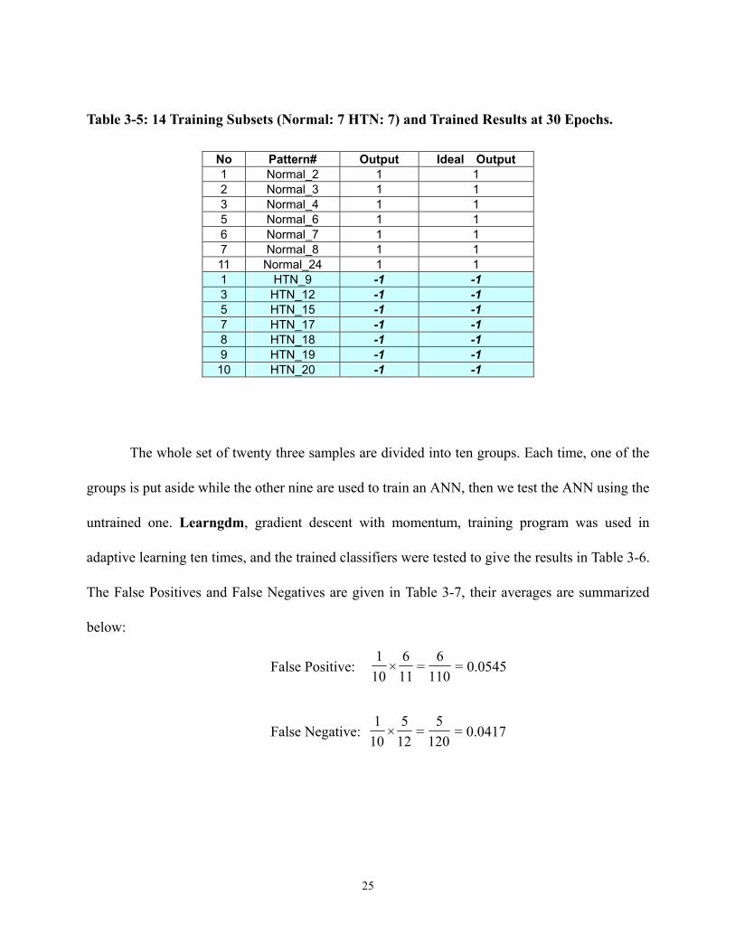
3.1.3 Jackknife Training and Error Estimation

Table 3-5 shows a subset of training data which we found can be used to successfully

train an ANN that correctly classifies the rest of the RV patterns. This was found by trial and

error using different combinations of subsets of RV patterns to train an ANN until no error was

found in the testing phase. Pattern Normal_2 and pattern HTN_15 were included because they

were misclassified by Fisher’s linear discriminant. Now they are correctly classified. This gives a

different satisfactory classifier. To gain a clear idea of the classification error rate, Jackknife

Error Estimation was analyzed.

ANN Final Weights with Momentum

Initial learning rate η = 0.01, α = 0.01 Iw{1,1}-Weight to layer 1 from input 1

[0.43221 -2.9578 9.1507 0.70229 -2.6536; -0.52917 0.36766 0.29635 0.40206 1.1181; 0.25125 1.2348 0.52256 0.111 0.45395]

Iw{2,1}-Weight to output layer [11.1691 12.949 -5.3405]

b{1}-Bias to layer 1 [3.5168; -12.5569; 4.815]

b{2}-Bias to layer 2 [-5.5975]

Table 3-4 Final Weights of the ANN Trained with Momentum by 23 RV Shape Samples.

25

The whole set of twenty three samples are divided into ten groups. Each time, one of the

groups is put aside while the other nine are used to train an ANN, then we test the ANN using the

untrained one. Learngdm, gradient descent with momentum, training program was used in

adaptive learning ten times, and the trained classifiers were tested to give the results in Table 3-6.

The False Positives and False Negatives are given in Table 3-7, their averages are summarized

below:

False Positive: 0545.0=110

6=

116

×101

False Negative: 0417.0=120

5=

125

×101

No Pattern# Output Ideal Output 1 Normal_2 1 1 2 Normal_3 1 1 3 Normal_4 1 1 5 Normal_6 1 1 6 Normal_7 1 1 7 Normal_8 1 1 11 Normal_24 1 1 1 HTN_9 -1 -1 3 HTN_12 -1 -1 5 HTN_15 -1 -1 7 HTN_17 -1 -1 8 HTN_18 -1 -1 9 HTN_19 -1 -1

10 HTN_20 -1 -1

Table 3-5: 14 Training Subsets (Normal: 7 HTN: 7) and Trained Results at 30 Epochs.

26

Jackknife Training and Error Estimates (with Momentum) Parts: 10 Hidden Neurons: 3 Output: 1 Features: 5

No Training data number Testing data set Training Test Results

Normal:1 HTN:-1 Normal HTN Total Normal HTN Total Wrong Epochs Correct Wrong

1 10 11 21 #2 #9 2 21 0 N#2 H#9 2 10 11 21 #3 #11 2 36 2 0 3 10 11 21 #4 #12 2 N#2 523 1 N#4 4 10 11 21 #5 #14 2 126 2 0 5 10 11 21 #6 #15 2 45 2 0 6 10 11 21 #7 #16 2 64 1 N#7 7 10 11 21 #8 #17 2 142 2 0 8 10 10 20 #10 #18#19 3 465 2 H#18

9 10 10 20 #13 #20#21 3 N#2

H#12 H#18

278 2 H#20

10 9 11 20 #23#24 #22 3 37 2 N#24

Times N: normal

H: HTN

Test

Result

Error

Rate Times

N: normal

H: HTN

Test

Result

Error

RateTimes

N: normal

H: HTN

Test

Result

Error

Rate

1 True N H 2 True N H 3 True N H

N(11) 10 1 1/11 N(11) 11 0 0 N(11) 9 2 2/11

H(12) 1 11 1/12

H(12) 0 12 0

H(12) 0 12 0

4 True N H 5 True N H 6 True N H

N(11) 11 0 0 N(11) 11 0 0 N(11) 10 1 1/11

H(12) 0 12 0

H(12) 0 12 0

H(12) 0 12 0

7 True N H 8 True N H 9 True N H

N(11) 11 0 0 N(11) 11 0 0 N(11) 10 1 1/11

H(12) 0 12 0

H(12) 1 11 1/12

H(12) 3 9 3/12

10 True N H

N(11) 11 0 1/11

H(12) 0 12 0

Table 3-7 False Positive and Negative Rates of Jackknife Training and Error Estimates of the ANN classification of RV Shape Data (using Learngdm in training).

Table 3-6 Jackknife Training and Error Estimates (with Momentum).

27

Next, we changed learngdm to learngd (the gradient descent without momentum) in

training and then went through the Jackknife error estimation again. The results are given in

Table 3-8 and Table 3-9. The average False Positive and average False Negative are

False Positive: 0454.0=110

5=

115

×101

False Negative: 0417.0=120

5=

125

×101

In this case, the False positive rate is slightly decreased; however, several patterns could not lead

to successful training or be classified correctly in testing.

Table 3-10 shows a supposed “optimal” training data. Such “difficult” patterns were picked

out in both cases, as marked by V in Table 3-10. These 11 samples were pooled together for

another training. The training without momentum was successful but the speed of convergence

was very slow. With the initial weights randomly chosen as given in Table 3-11, all RV patterns

were correctly classified; the resulting weight vectors and bias values are given in Table 3-12.

The training with momentum was faster, it took only 2840 epochs as shown in the learning curve

in Figure 3-5, however, misclassified one pattern in testing. Figure 3-6 shows the training

patterns in the x1-x2 (Global S/V vs. 0-25%S/V) plane. From the plot we can see that these

patterns are located close to the border of the two classes and are expected to be difficult to train.

We call this subset as “optimal” training subset. If we can successfully train an ANN with these

samples, we expect the testing performance would show the least error rate. This subset lies

inside the subset of 14 samples given in Table 3-5 but obtained other than trial-and-error.

28

Jackknife Training and Error Estimates (without Momentum) Parts: 10 Hidden Neurons: 3 Output: 1 Features: 5

No Training data number Testing data set Training Test Results Normal:1 HTN:-1

Normal HTN Total Normal HTN Total Wrong Epochs Correct Wrong

1 10 11 21 #2 #9 2 50000 0 N#2 H#9

2 10 11 21 #3 #11 2 50000 1 N#3

3 10 11 21 #4 #12 2 50000 0 N#4 H#12

4 10 11 21 #5 #14 2 50000 2 0 5 10 11 21 #6 #15 2 50000 2 0 6 10 11 21 #7 #16 2 50000 1 N#7 7 10 11 21 #8 #17 2 50000 2 0

8 10 10 20 #10 #18 #19 3 H#12 50000 2 H#19

9 10 10 20 #13 #20 #21 3 50000 3 0

10 9 11 20 #23 #24 #22 3 50000 2 N#24

H#22

Times N: normal

H: HTN

Test

Result

Error

Rate Times

N: normal

H: HTN

Test

Result

Error

RateTimes

N: normal

H: HTN

Test

Result

Error

Rate

1 True N H 2 True N H 3 True N H

N(11) 10 1 1/11 N(11) 10 1 1/11 N(11) 10 1 1/11

H(12) 1 11 1/12

H(12) 0 12 0

H(12) 1 11 1/12

4 True N H 5 True N H 6 True N H

N(11) 11 0 0 N(11) 11 0 0 N(11) 10 1 1/11

H(12) 0 12 0

H(12) 0 12 0

H(12) 0 12 0

7 True N H 8 True N H 9 True N H

N(11) 11 0 0 N(11) 11 0 0 N(11) 11 0 0

H(12) 0 12 0

H(12) 2 10 2/12

H(12) 0 12 0

10 True N H

N(11) 10 1 1/11

H(12) 1 11 1/12

Table 3-9 False Positive and Negative Rates of Jackknife Training and Error Estimates of the ANN classification of RV Shape Data (using Learngd in training).

Table 3-8 Jackknife Training and Error Estimates (without Momentum).

29

Normal No Training error#

# A. Momentum

B. Without

momentum

Optimal Training Data

Based on combination of

A&B 2 1 V V V 3 2 V V 4 3 V V V 5 4 6 5 7 6 V V V 8 7

10 8 13 9 23 10 24 11 V V V

HTN 9 1 V V V 11 2 12 3 V V V 14 4 15 5 16 6 17 7 18 8 V V 19 9 V V 20 10 V V 21 11 22 12 V V V

Total 9 9 11

ANN Initial Weights without Momentum

Initial learning rate η = 0.01 Iw{1,1}-Weight to layer 1 from input 1

[0.48063 -0.0054258 -0.017489 -0.12276 0.24704; -0.24552 0.12954 -0.16544 0.21916 0.11931; 0.11594 0.1031 0.13123 0.65863 -0.19268]

Iw{2,1}-Weight to output layer [-0.21634 0.99912 0.95653]

b{1}-Bias to layer 1 [-6.5624; -0.19483; -2.9812]

b{2}-Bias to layer 2 [0]

Table 3-10 “Optimal” Training Subset Derived from Two Jackknife Error Estimations.

Table 3-11 ANN Initial Weights Trained by 11 Optimal Sample.

30

ANN Final Weights without Momentum

Initial learning rate η = 0.01 Iw{1,1}-Weight to layer 1 from input 1

[-0.053048 -0.21676 1.2021 -0.40867 -0.70051; 0.17839 1.001 -0.51442 -0.69621 -0.092139; -0.054465 -0.25143 0.15553 -0.72695 -0.2211]

Iw{2,1}-Weight to output layer [1.7635 -1.3617 -1.9717]

b{1}-Bias to layer 1 [6.0173; -2.0344; 8.5413]

b{2}-Bias to layer 2 [1.38]

Table 3-12 ANN Final Weights Trained by 11 Optimal Sample.

Figure 3-5 Learning Curve (with momentum) of ANN Trained by 11 Optimal Data.

31

Figure 3-6 Two dimensional plot of “Optimal” Training Samples (Bold) Given in Table 3-10.

32

3.2 RADIAL BASIS FUNCTION NETWORKS

Radial basis function (RBF) network is one type of feedforward artificial neural network

where the interpolation nonlinear activation function in each neural unit is given by a symmetric

function of the form

(3-12).

The argument of the function is the Euclidean distance of the input vector x from a center vector

ci, which gives the name radial basis function. Two choices of the function f are

, i = 1,…, k (3-13),

, i = 1,…, k (3-14).

The Gaussian form (3-13) is more widely used. With a sufficiently large k, the decision function

g(x) can be approximated by a linear combination of k RBFs where each is located at a different

point in the space [12] [13] (3-15),

where y is the output vector of k RBFs. Note that g(x) is locally maximum when x = ci. The

center vector ci = c1i, …, cNi of the ith hidden neuron has N components to match the input

feature vector. The parameter σi in Equation (3-13) is used to control the spread of the radial

2

2

2=)( i

ix－－

exf σ

c

22

2

+=)(

ix－xf

cσ

σ

byw

bewxg

T

xx－k

ii

i

iT

i

+=

+==

c(c(22

)－)－

1∑)( σ

)c( i－xf

33

basis function so that its value decreases more slowly or more rapidly as x moves away from the

center vector ci, that is, as )c ii－x increases.

A radial basis function network contains the following: (a) an input layer of d branching

nodes, one for each feature component xi; (b) a hidden layer of M neurons where each neuron has

the radial basis function ym = fm(x) as its activation function centered at a cluster center in the

feature space; and (c) an output layer of J neurons that sum up the outputs yi from the hidden

neurons, that is, each output layer neurons with output zj uses a linear activation function

∑=

+=M

mjmmjj bywz

1 (3-16).

Figure 3.6 shows the block diagram of a general RBF network.

Figure 3-7 Block Diagram of a RBF Network.

Inputs

…

x1

x2

xd

…

Outputs

…

z1

zJ

c11

CNi

c1i

f1(*)

f2(*)

fM(*)

cN1

w11

wMJ

wM1

b1

bJ

t1

tJ

…

Targets

y1

y2

yM

34

In multilayer perceptrons, each hidden neuron reveals a linear combination of input

features, ii xw∑ , its output will be the same for all x lying on a hyperplane =ii xw∑ a constant.

On the other hand, in the RBF networks, the output of each RBF neuron is the same for all x’s

that are equally distant from its center ci and decreases exponentially (for Gaussians) with the

distance. In other words, the activation responses of the neurons are of a local nature in RBF

networks and of a global nature in multilayer perceptron networks. This difference makes great

consequences on both the speed of convergence in training and the performance of generalization.

Mainly, multilayer perceptrons learn slower than RBF networks. Simulation results have [14]

shown that, in order to achieve a performance similar to that of multilayer perceptrons, an RBF

network should be of much higher order. The reason is the locality of the RBF activation

functions, which makes it necessary to use a large number of centers to fill in the input space in

which g(x) is defined, and there is an exponential dependence between this number and the

dimension of the input space.

The training of a RBF network involves learning these sets of parameters: cm, 2mσ , (m =

1, 2, …, M), and connection weights wmj, (m = 1, 2, …, M, j = 1, 2, ,…, J), from hidden neurons

to output neurons. The number of RBF to be used must be heuristically determined first. Use a

set of Q training samples, xq, (q = 1, 2, …, Q), we define the total sum squared error E over all Q

samples,

2

1 1)( q

j

Q

q

J

j

qj ztE −=∑∑

= =

(3-17),

and use the steepest descent for iteratively adjusting those parameters [15]:

35

mjmjmj w

Ekwkw∂∂

−=+ 1)()1( η

d) ..., 2, 1, ( ,)()1( 2 =∂∂

−=+ icEkckcmi

mimi η (3-18).

2322 )()1(

mmm

Ekkσ

ησσ∂∂

−=+

3.2.1 Training

A specific choice for the initial centers was suggested [16] in some cases considering the

problem nature. These centers may be selected randomly from the training set which is presumed

to be distributed in a meaningful manner over the input feature space.

For the right ventricle shape classification, only one output neuron is needed for two

classes (normal and HTN), furthermore, it is not necessary to have a bias b0. For the small size of

the training set that we have, choosing the initial centers randomly from the training samples

often failed to succeed to give a satisfactory decision function. We performed an exhaustive

experimental study on the training and finally used 11 RBFs with the same spread σ. A total of

[5×11 + 11 + 1 = 67] parameters were trained. Using all 23 training samples, the successfully

trained network is given by the parameters listed in Table 3-13. The training convergence was

reached in 11 epochs (see Figure 3-7). The decision function is given by

2c-x

2111

1

i2)( σ−

=∑= ewxgi

m (3-19).

36

Table 3-13 Final Weights of RBF Network.

Final Weights of RBF network σ = 0.1, η1 = 1.6, η2 = 1, η3 = 1,

Iw{1,1}-Weight to layer 1 from input 1 [4.68 4.85 3.87 3.7 10.26; 6.18 11.17 4.92 5.81 8; 9.57 19.36 17.85 5.66 7.84; 7.62 18.08 9.73 5.83 6.02; 7.65 14.61 7.87 6.24 6.48; 7.04 13.49 6.88 5 12.19; 7.92 17.79 11.37 5.69 8.59; 7.58 13.38 6.08 6.86 8.95; 7.43 18.66 10.16 5.33 9.37; 8.96 20.9 12.85 5.65 10.42; 6.17 18.39 8.95 5.18 4.6]

Iw{2,1}-Weight to layer

[1 1 1 1 1 1 1 1 1 1 1]

Figure 3-8 Learning Curve of the RBF Network.

37

3.2.2 RBF Jackknife Error Estimation

Table 3-14 shows the Jackknife error analysis result of our RBF network. The False

Positive and False Negative are

False Positive: 0454.0=110

5=

115

×101

False Negative: 0417.0=120

5=

125

×101

These two values are about the same as that obtained from the ANN trained without momentum

except here the speed of convergence is much faster.

Times N: normal

H: HTN

Test

Result

Error

Rate Times

N: normal

H: HTN

Test

Result

Error

RateTimes

N: normal

H: HTN

Test

Result

Error

Rate

1 True N H 2 True N H 3 True N H

N(11) 10 1 1/11 N(11) 11 0 0 N(11) 11 0 0

H(12) 0 12 0

H(12) 1 12 1/12

H(12) 1 11 1/12

4 True N H 5 True N H 6 True N H

N(11) 10 1 1/11 N(11) 10 1 1/11 N(11) 11 0 0

H(12) 0 12 0

H(12) 0 12 0

H(12) 1 11 1/12

7 True N H 8 True N H 9 True N H

N(11) 11 0 0 N(11) 10 1 1/11 N(11) 10 1 1/11

H(12) 1 11 1/12

H(12) 0 11 0

H(12) 0 12 0

10 True N H

N(11) 11 0 0

H(12) 1 11 1/12

Table 3-14 False Positive and Negative Rates of RBF Jackknife Error Estimates.

38

3.3 SUMMARY OF RESULTS

Our experimental results show that the speed of convergence of the ANN (with sigmoidal

functions) is much slower than the RBF network. However, in our ANN, only 3 hidden neurons

are used versus 11 hidden neurons required in our RBF network for correct classification of all

the training samples. With the small size of our training set, data distribution is unclear, so the

RBF network needs more than triple hidden neurons. The number of parameters to be trained is

many more, hence the trained result would be less certain.

A sigmoidal neuron can respond over a large region in the input space, while a radial

basis neuron only responds to a relatively small region in the input space. Hence the larger is the

input space (in terms of the number of inputs and the range in which those inputs may vary),

more radial basis neurons are required. In the next chapter, we will discuss our study on training

support vector machines employing RBF neurons and sigmoidal neurons.

39

4.0 SUPPORT VECTOR MACHINES

The idea behind the support vector machines is to look at the RBF network as a mapping

machine, through the kernels, into a high dimensional feature space. Then a hyperplane linear

classifier is applied in this transformed space utilizing those patterns vectors that are closest to the

decision boundary. These are called support vectors corresponding to a set of data centers in the

input space. The hyperplane in this feature space (or the nonlinear decision surface in the original

space) will be optimized in giving the largest tolerance margin. The algorithm computes all the

unknown parameters automatically including the number of these centers. In the last decade,

significant advances have been made in support vector machine (SVM) research [17], both

theoretically using statistical learning theories [18], [19], and algorithmically based on

optimization techniques [20]. Since this is a relatively new design methodology for pattern

classification, we give a substantially detailed review in this section, and then present a case

study on right ventricle shape data.

4.1 LINEAR SUPPORT VECTOR MACHINES

Consider the 2-class problem and suppose that N training samples {xi} are given which

are linearly separable in the feature space. Let the class index be denoted by ti (i = 1, 2), where ti

=1 for patterns of class 1 and ti =2 for patterns of class 2. ti also represents the desired target

output, then, we denote the training samples by Niii tx 1=)},{( .

40

A linear separating plane is given by

g(x) = wTx +b = 0 (4-1),

where w is a weight vector and b is a bias which determines its location related to the origin of

the input space. For a given w and b, the margin of separation denoted by r is defined as the

separation between the hyperplane in Eq. (4-1) and the closest data point as shown in Fig. 4-1,

To find the optimal separating hyperplane with the largest margin is the goal of training a support

vector machine. We expect that the larger the margin is, the better the classifier will be. Let wo

and bo denote the optimal values of the weight vector and bias, respectively, the optimal

hyperplane is then given by g(x) = wo

Tx + bo = 0 (4-2).

The distance from a hyperplane to a pattern x is given by

owxg

r)(

= (4-3),

then, for all training patterns x,

0)( >=+= ooTo wrbxwxg (4-4),

we want to find the weight vector wo and bo that maximizes r. The solution can be arbitrarily

scaled, so we may put the constraint after an appropriate scaling as

1≥+ oiTo bxw for ti = +1

1≤+ －bxw oiTo for ti = -1

),54( ﹣

41

Figure 4-1 Two out of Many Separating Lines: Upper, a Less Acceptable One with a Small Margin, And Below, a Good One with a Large Margin.

Class 1, t = +1

Class 2, t = －1

Small margin x2

x1

Class 1, t = +1

Class 2, t = －1

Large margin

x2

x1

Decision boundaries

r

r

42

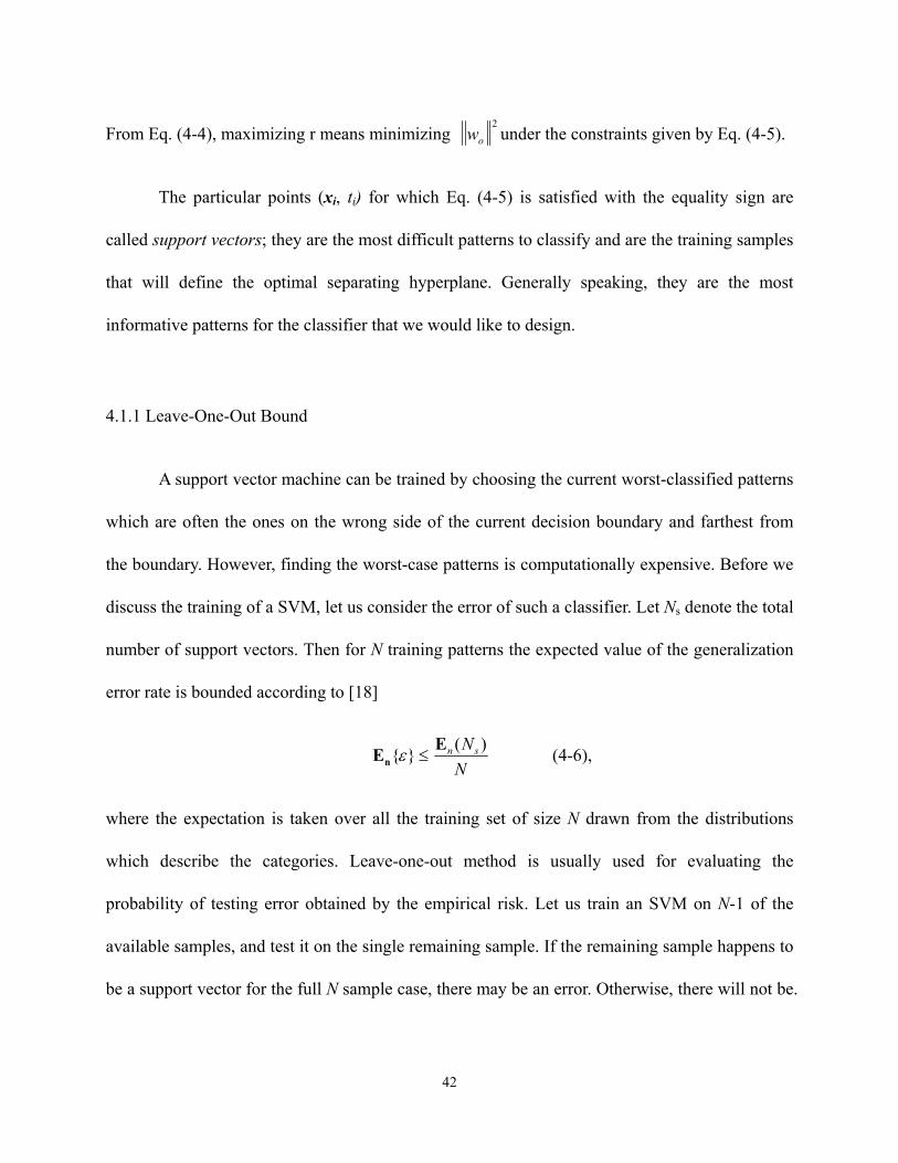
From Eq. (4-4), maximizing r means minimizing 2

ow under the constraints given by Eq. (4-5).

The particular points (xi, ti) for which Eq. (4-5) is satisfied with the equality sign are

called support vectors; they are the most difficult patterns to classify and are the training samples

that will define the optimal separating hyperplane. Generally speaking, they are the most

informative patterns for the classifier that we would like to design.

4.1.1 Leave-One-Out Bound

A support vector machine can be trained by choosing the current worst-classified patterns

which are often the ones on the wrong side of the current decision boundary and farthest from

the boundary. However, finding the worst-case patterns is computationally expensive. Before we

discuss the training of a SVM, let us consider the error of such a classifier. Let Ns denote the total

number of support vectors. Then for N training patterns the expected value of the generalization

error rate is bounded according to [18]

NNsn )(}{ EEn ≤ε (4-6),

where the expectation is taken over all the training set of size N drawn from the distributions

which describe the categories. Leave-one-out method is usually used for evaluating the

probability of testing error obtained by the empirical risk. Let us train an SVM on N-1 of the

available samples, and test it on the single remaining sample. If the remaining sample happens to

be a support vector for the full N sample case, there may be an error. Otherwise, there will not be.

43

If there exists a SVM that that will separates all the samples successfully, and the number of

support vectors is small, then the expected error rate given in Eq. (4-6) will be low.

Figure 4-1 compares the idea that a classifier with a smaller margin will have a higher

expected risk. The dashed separation line shown in the lower graph will promise a better

performance in generalization than the dashed decision surface having a smaller margin shown in

the upper graph.

4.1.2 Training a SVM

Return to the margin maximization (or 2ow minimization) problem discussed earlier, we

consider the cost function to be minimized:

www T

21)( =Ψ

We want to find an optimal hyperplane specified by (wo, bo) using the training sample set

Niii tx 1=)},{( .

Under the constraints in Eq. (4-5) which is equivalent to

1≥)+( bxwt iT

i for i = 1,2, …, N (4-7),

using Lagrange multipliers [21] we convert the constrained optimization problem into an

unconstrained minimization problem by constructing the cost function

－1])([－21),,(

1

bxwtwwbwJ iT

i

N

ii

T += ∑=

αα (4-8),

44

where auxiliary nonnegative variables αi ≥ 0 are called Lagrange multipliers. We seek to

minimize J(∙) with respect to the weight vector w and b, and maximize it with respect to αi ≥ 0.

The last term in Eq. (4-8) expresses the goal of classifying the training sample correctly. It can be

shown that using the Kuhn-Tucker construction that this optimization can be reformulated as

maximizing a dual form

jTijij

N

ji

N

i

N

ii xxttQ αααα ∑∑∑

===

=111 2

1－)( (4-9),

subject to the constraints

(1) 01

=∑=

i

N

iitα

(2) αi ≥ 0 for i = 1, 2, …, N

4.2 LINEAR SOFT MARGIN CLASSIFIER FOR OVERLAPPING PATTERNS

Now let us consider the case of sample patterns that not linearly separable. To find a

hyperplane with a maximal margin, we must allow some sample (or samples) to be unclassified,

i.e., on the wrong side of a decision boundary. In this case, we would like to find an optimal

hyperplane that minimizes the probability of classification error, averaged over the training set.

Thus, we will allow a soft margin, and those samples inside this margin are ignored. The width

of a soft margin will be controlled by a regularization or corresponding penalty parameter C that

determines the trade-off between the training error and the so called VC dimension of the model.

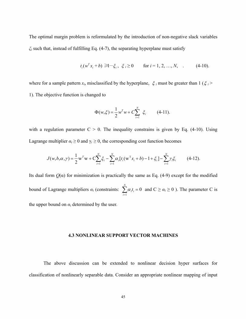
45

The optimal margin problem is reformulated by the introduction of non-negative slack variables

ξi such that, instead of fulfilling Eq. (4-7), the separating hyperplane must satisfy

iiT

i －bxwt ξ1≥)+( , ξ i ≥ 0 for i = 1, 2, …, N, . (4-10).

where for a sample pattern xi, misclassified by the hyperplane, ξ i must be greater than 1 (ξ i >

1). The objective function is changed to

∑=

+=ΦN

ii

T Cwww12

1),( ξξ (4-11).

with a regulation parameter C > 0. The inequality constrains is given by Eq. (4-10). Using

Lagrange multiplier αi ≥ 0 and γi ≥ 0, the corresponding cost function becomes

∑∑∑===

−+−+−+=N

iiiiii

N

ii

N

ii

T bxtbwJ1

T

11

]1)w([Cww21),,,( ξγξαξγα (4-12).

Its dual form Q(α) for minimization is practically the same as Eq. (4-9) except for the modified

bound of Lagrange multipliers αi (constraints: 01

=∑=

N

iiitα and C ≥ αi ≥ 0 ). The parameter C is

the upper bound on αi determined by the user.

4.3 NONLINEAR SUPPORT VECTOR MACHINES

The above discussion can be extended to nonlinear decision hyper surfaces for

classification of nonlinearly separable data. Consider an appropriate nonlinear mapping of input

46

vectors into a high-dimensional feature space illustrated in Fig. 4-2 such that an optimal

hyperplane can be constructed in this space. This will lead to a nonlinear support vector machine

giving optimal nonlinear hypersurface in the input space.

4.3.1 Inner-Product Kernel

Let { Mjj 1)x( =ϕ } denote a set of nonlinear transformations from the input space to the

feature space: M is the dimension of the new feature space. Given such a set of nonlinear

transformations, we may define a hyperplane acting as the decision surface as follows:

0)x(1

=+∑=

bw j

M

jjϕ (4-13),

Input (data) space

Feature space

ix

)( ixϕ

)(•ϕ

Figure 4-2 Nonlinear Mapping )(•ϕ from the Input Space to a High-Dimensional Feature Space.

47

where { } Mjjw 1= denotes a set of weights connecting the new feature space to the output space,

and b is the bias. Augmented by 1=)(0 xϕ for all x and w0 as the bias b, Eq. (4-13) becomes

0)x(0

=∑=

j

M

jjw ϕ (4-14),

Define the vector

φ(x) TM )]x(),...,x(),x([ 10 ϕϕϕ= (4-15),

and the augmented weight vector

TMwww ] ..., ,,[w 10= , (4-16),

then the decision surface is given by

Tw φ(x) = 0 (4-17).

We now seek the linear separability in the feature space φ(x). Let

i

N

iit∑

=

=1

w α φ(xi) (4-18),

where the feature vector )( ixϕ corresponds to the ith input sample xi. Substituting Eq. (4-18)

into (4-17) defines a decision surface computed in the feature space as:

i

N

ii t∑

=1α φT(xi) φ(x) = 0 (4-19).

48

The term φT(xi) φ(x) represents the inner product of two (M+1)-dimensional vectors induced in

the feature space by an input vector x and the ith training sample xi. Now, let M = N and the

inner-product kernel K(x, xi) be formed from all N training samples (φ(x) be a (N+1)×1 vector)

K(x, xi) = φT(x) φ(xi)

= )x()x(0

ijj

N

jϕϕ∑

=

for i = 1, 2, …, N (4-20),

The inner-product kernel is a symmetric function of its arguments, as shown by K(x, xi) = K(xi, x)

for all i. Now we can use the inner-product kernel K(x, xi) to construct the optimal hyperplane in

the new feature space without having to consider the feature space itself in explicit form. The

optimal hyperplane is now given by

i

N

iit∑

=1

α K(x, xi) = 0 (4-21).

Type of support vector

machine

Inner product kernel K(x, xi), i = 1,2, …, N Note

Radial basis function network 2

21

2 i－－

exx

σ The width σ2, common to all the kernels, is specified by the user.

Two-layer perceptron tanh(β0xTxi + β1)

Mercer’s theorem (see Appendix B)

is satisfied only for some values of

β0 and β1.

Table 4-1 Specifications of Inner-Product Kernels.

49

4.3.2 Construction of a SVM

We can use the expansion of the inner-product kernel K(x, x′) in (4-20) to construct a

decision surface that is nonlinear in the input space but linear in the new feature space.

Following Eq. (4-19) and replacing the inner-product jT xxi

by the inner-product kernel K(xi, xj)

= φT(xi) φ(xj). The dual form of the constrained optimization for a nonlinear support vector

machine is stated as follows [22]:

Given the training sample set Niii tx 1=)},{( , find the Lagrange multipliers N

ii 1=}{α that

maximizes the objective function

)x,x(21)(

111jijiji

N

j

N

ii

N

iKtt－Q αααα ∑∑∑

===

= (4-22),

subject to the constrains:

(1) 01

=∑=

ii

N

itα

(2) Ci ≤≤0 α for i = 1, 2, … , N

where C is a user-specified positive parameter and also the upper bond of iα , K(x, x′) can be

viewed as the ij-th element of a symmetric N-by-N matrix K as shown by

K = {K(xi, xj)} Nji 1),( = (4-23).

50

α1t1

α2t2

αNtN

Compute the optimum values of the Lagrange multipliers, iα (i = 1, 2, …, N). The weight

vector w, connecting the new feature space to the output space is computed by

∑=

=N

iiitw

1α φ(xi) (4-24).

The block diagram of a nonlinear SVM is shown in Fig. 4-3.

Hidden layer of N Inner-product kernels K(x, xj) =φ(x) φ(xj), j = 1, 2, …, N

Figure 4-3 Block Diagram of a Nonlinear SVM for Training.

K(x,x1)

K(x,x2)

K(x,xN)

Output

Bias b

Input layer of dimension d Use N training samples

x1

x2

xd

Input vector

x

Linear outputs

y

… …

w0

51

4.4 SUPPORT VECTOR MACHINES FOR RIGHT VENTRICLE SHAPE CLASSIFICATION

The method discussed above was applied to design SVM machines for classification of

right ventricle shape measurements into normotensive or hypertensive (HTN) class [23]. We

considered two kinds of kernel functions, Gaussian kernel, K(x, xi) = 2

21

2 i－－

exx

σ , and sigmoidal

kernels K(x, xi) = tanh(β0xTxi + β1), as listed in Table 4-1. All 23 sample patterns of 5 dimensions

({xi, ti = 1 | i = 1, 2, …, 11}, normal; { xi, ti = －1 | i = 12, 13, …, 23}, HTN), as given in

Appendix A, were used in training, so initially there are 23 units in the hidden layer of the SVM.

For the SVM using Gaussian kernels (with σ = 1 in all units), experiments were made

using different values of regularization parameter C. Note that Gaussian kernels do not

necessarily require a bias term in the decision function g(x), in this case, the equality constraint

01

=∑=

ii

N

itα (which is resulted from 0=

∂∂

bJ ) does not exit. The computed iα (i = 1, 2, …, 23)

under C = 100 are shown in Table 4-2. There are 8 support vectors, those are training patterns

for which 0 < iα < C as marked by V in the Table. All other patterns ( iα = 0) are outside the

margin strip. The set of support vectors (SV) are (x1, x2, x6, x11, with ti = 1) and (x12, x14, x20, x22,

with ti = －1). The decision function is given by

g(x) = α1K(x,x1) + α2K(x,x2) + α6K(x,x6) + α11K(x,x11)－α12K(x,x12)－α14K(x,x14)－α20K(x,x20)

－α22K(x,x22) (4-25),

52

where K(x, xi) = )x()x(

21

2 iT

i xx－

e−−

σ

The tolerance margin is r = w1 . Since the expression of φ(x) was not explicitly given,

weight vector ∑=

=N

iiit

1

w α φ(xi) was not computed. However, 2w was computed via

Kernel: Gaussian, σ= 1, C=100

No. αi SVM 1 7.9237 V 2 14.2993 V 3 0.0000 4 0.0000 5 0.0000 6 10.6449 V 7 0.0000 8 0.0000 9 0.0000 10 0.0000

Normal

11 3.1767 V 12 4.8679 V 13 0.0000 14 7.9043 V 15 0.0000 16 0.0000 17 0.0000 18 0.0000 19 0.0000 20 19.4704 V 21 0.0000 22 1.1980 V

HTN

23 0.0000

Table 4-2 Results of SVM with Gaussian Kernels.

53

α1t1

α2t2

αNtN

26).-(4 ),()]()(

)]([)]([www

j

T2

ijiij i

jjijT

iijSVj SVi

iii

iT

jjj

j

xxKttxxtt

xtxt

ααϕϕαα

ϕαϕα

∑∑∑ ∑

∑∑

==

==

∈ ∈

Using the determined support vectors gives 2w = 17.3712, hence, the tolerance margin is

2w

1r = = 0.23993.

Hence, we only need 8 hidden units, instead of 23, in the trained classifier as shown in Figure

4-4. The decision boundary in x1-x2 (Global S/V, 0-25%S/V) plane with the projection of

sample patterns are shown in Figure 4-5. A small margin is noticed in the graph.

Hidden layer of 8 Inner-product kernels K(x, xj) =φ(x) φ(xj), j = 1, 2, …, 8

Figure 4-4 Block Diagram of the Trained SVM.

K(x,x1)

K(x,x2)

K(x,x8)

Output

Bias b=0

Input layer of dimension d Use N testing samples

x1

x2

xd

Input vector

x

Linear outputs

y

… …

w0

54

Figure 4-5 Decision Boundary in x1-x2 (Global S/V, 0-25%S/V) Plane with the Projection of Sample Patterns.

HTN margin

Normal margin

Normal margin

Decision boundary

Global S/V

0-25

%S/

V

55

We performed the leave-one-out testing of this SVM by training on 22 samples and testing on the

left-out 1 sample, rotated 23 times. The results are given in Table 4-3. The training was

successful each time; there was 1 error in testing some time, whenever it was one of the support

vectors obtained in the full training (training all 23 samples). The average false positive and

average false negative are 0.01186 (=113

231× ) and 0.00725 (=

122

231× ); 3 samples are classified

correctly but with the margin strips.

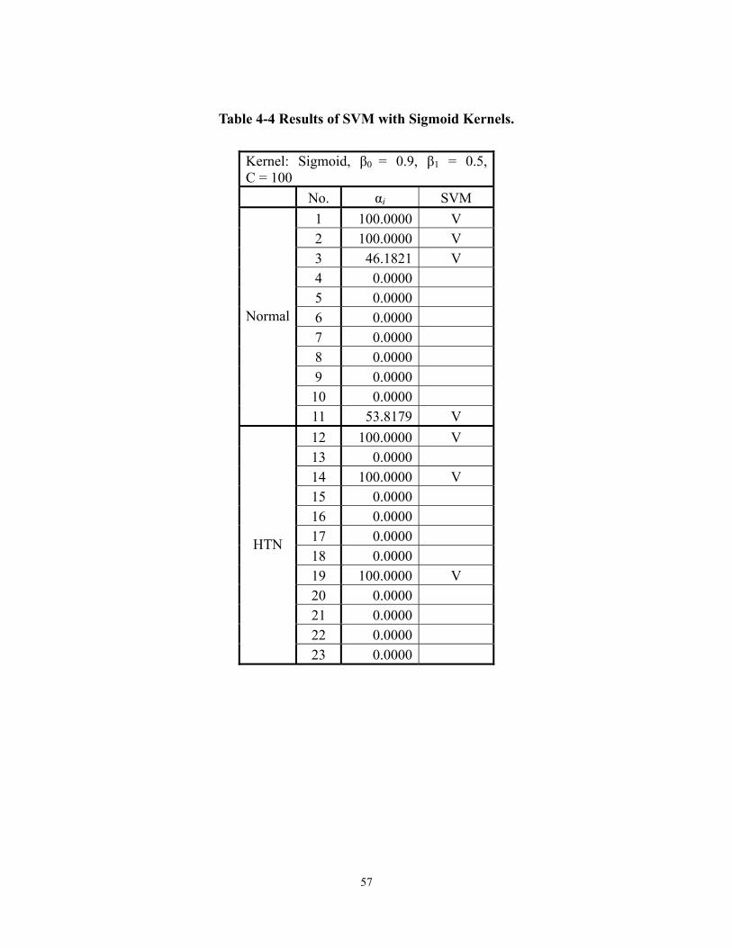
The other SVM used sigmoidal kernel with β0 = 0.9 and β1 = 0.5, the computed iα ’s

under C = 100 are listed in Table 4-4. There appears to have seven support vectors ( iα > 0), five

of which computed to iα = C = 100 (i = 1, 2, 3, 11, 12, 14, 19). Only two support vectors

corresponding to iα < C. For those samples xi having iα = C = 100, the corresponding slack

variables ξi may be greater than 0 or even 1; ξi can be computed from tig(xi) = 1－ξi. For ξi > 1,

the training sample must be misclassified; for 1 > ξi > 0, the sample was correctly classified but

close to the hyperplane with a distance less than the margin.

Compare the support vectors found in each SVM with the “optimal” training data found

by the Jackknife analysis of ANN (Table 3-10), it is not surprising that all the support vectors

(except pattern No. 14) of the SVM with sigmoidal kernels are members of that “optimal”

training data. Similarly, the support vectors of the SVM with Gaussian kernels also coincide with

that set except for pattern No. 14.

56

Testing Pattern no. (value) Times

Leave out (testing)

Pattern No. No. of SV

Error With margin strip value

Correctvalue

1. 1. 6 1(-2.3185) 2. 2. 9 2(-0.7958) 3. 3. 8 1.1846 4. 4. 8 2.8205 5. 5. 8 3.2176 6. 6. 9 6(-1.2802) 7. 7. 8 3.1304 8. 8. 8 3.1912 9. 9. 8 3.0087 10. 10. 8 2.4327 11. 11. 8 11 0.2091 12. 12. 8 12 -0.0935 13. 13. 8 -1.970814. 14. 8 14(1.6830) 15. 15. 8 -2.852516. 16. 8 -1.796217. 17. 8 -2.048718. 18. 8 -2.844319. 19. 8 -2.677920. 20. 8 20(0.1423) 21. 21. 8 -2.898322. 22. 7 22 -0.0437 23. 23. 8 -2.0673

Table 4-3 Result of Leave-One-Out Testing.

57

Kernel: Sigmoid, β0 = 0.9, β1 = 0.5, C = 100 No. αi SVM

1 100.0000 V 2 100.0000 V 3 46.1821 V 4 0.0000 5 0.0000 6 0.0000 7 0.0000 8 0.0000 9 0.0000 10 0.0000

Normal

11 53.8179 V 12 100.0000 V 13 0.0000 14 100.0000 V 15 0.0000 16 0.0000 17 0.0000 18 0.0000 19 100.0000 V 20 0.0000 21 0.0000 22 0.0000

HTN

23 0.0000

Table 4-4 Results of SVM with Sigmoid Kernels.

58

5.0 CONCLUSIONS AND FUTURE WORK

The case study conducted in this project is concerned with the classification of right

ventricle shape measurements obtained from MRI sequences, to either normal or hypertensive

classes. Pediatricians are interested in diagnosis on possible congenital heart defects, especially

those associated with pressure and volume overload problems. The samples are given in

5-dimensional data, and only a small sample set are available. To develop a suitable pattern

classifier, we went through first the Fisher linear discriminant and the linear classifier trained by

the Ho-Kayshap algorithm. The results showed that the sample data are nonlinearly separable.

We then focused on training of feedforward artificial neural networks using sigmoidal functions

and radial bias functions, considering the feature dimensions, small sample size and the limit on

the number of neurons to be used, we succeeded in training an ANN having only three hidden

neurons (with sigmoidal nonlinearity) and one output neuron, and a RBF network with 11

Gaussian basis functions, all with 100% classification capability. Jackknife training and error

estimation were performed in both cases. The issues attacked are the minimum number of units

needed and the associated minimum number of parameters to be trained in comparison to an

earlier study. In order to minimize the structural risk, we next considered support vector

machines and trained nonlinear classifiers with minimum number of hidden neurons giving

certain tolerance margins.

59

The artificial neural network using back-propagation training suffers from its slow

convergence. They may have larger testing (statistic) errors as compared to support vector

machines due to the Empirical Risk Minimization (ERM) approach employed by the former.

The RBF network converges with an amazing speed. Nevertheless, with the small amount of

available RV shape data for training, we were unable to reduce the number of hidden neurons

used in the RBF network.

Although the SVM uses as many kernels during the training as the number of training

samples when it maps nonlinearly the original data into new feature space, its support vectors

were quickly found and the optimal separating surface gave the best possible tolerance margin.

The resulting number of hidden neurons used is 8, more than that used in the ANN. It implies

the minimization of structure risk (SRM) and minimizing the number of neural units used,

through minimizing an upper bound on the generalization error as opposed to ERM which

minimizes the error on the training data. Our experimental results on the case study have shown

that although the ANN (sigmoidal) and SVM are comparable in performance, SVM has a

greater potential to generalize in statistical learning. We would like to gather more training data

to carry out further studies on the right ventricle shape classification. We also would like to

investigate the automatic segmentation of right ventricles from cardiac MRI sequences to

obtained real world data with the goal of developing a fully automatic pattern recognition

system.

60

APPENDIX A

Sample Shape Features (Surface/Volum Ratio)

# No. Global S/V 25% 50% 75% 100%

2 1 4.68 4.85 3.87 3.70 10.26 3 2 6.18 11.17 4.92 5.81 8. 4 3 9.57 19.36 17.85 5.66 7.84 5 4 7.62 18.08 9.73 5.83 6.02 6 5 7.65 14.61 7.87 6.24 6.48 7 6 7.04 13.49 6.88 5. 12.19 8 7 7.92 17.79 11.37 5.69 8.59 10 8 7.58 13.38 6.08 6.86 8.95 13 9 7.43 18.66 10.16 5.33 9.37 23 10 8.96 20.90 12.85 5.65 10.42

Normal

24 11 6.17 18.39 8.95 5.18 4.60 9 12 5.67 14.12 7.46 4.85 4.78 11 13 4.83 9.68 3.90 4.02 8.18 12 14 6.77 11.12 5.58 5.89 14.13 14 15 5.22 10.43 5.16 3.91 5.63 15 16 5.22 10.90 4.36 3.84 9.09 16 17 5.15 11.81 5.11 4.11 8.52 17 18 5.19 11.33 4.86 3.87 6.31 18 19 5.35 9.23 7.34 3.80 4.56 19 20 5.82 10.46 4.82 4.82 9.08 20 21 4.31 14.02 4.18 3.36 4.54 21 22 3.25 4.94 2.90 2.79 4.18

HTN

22 23 5.65 10.77 5.01 4.49 6.38

Table A-1 Sample Right Ventricle Shape Data Obtained from MRI Sequences with 11 Normal and 12 Hypertensive (HTN) Cases. Five Features Consist of Global and Four Regional Surface/Volum Ratios [2].

# is the sample number assigned in Reference [2].

61

APPENDIX B

Mercer’s Theorem

The expansion of Eq. (4-20) for the inner-product kernel K(x, xi) is an important special

case of Mercer’s theorem that arises in functional analysis [19]. Let K(x, x′) be a continuous

symmetric kernel that is defined in the closed interval a ≤ x ≤ b and likewise for x′. The kernel

K(x, x′) can be expanded in the series form

K(x, x′) = )x'()x(1

iii

i ϕϕλ∑∞

=

(4-22),

with positive coefficientsλi > 0 for all i. For this expansion to be valid and for it to converge

absolutely and uniformly, it is necessary and sufficient that the following condition

0≥')'()()',(∫∫ xxxxxxa

b

a

bddK ψψ

holds true for all )(•ψ for which

∞<)(2∫ xxa

bdψ

The functions are called eigenfunctions of the expansion and the numbersλi are

eigenvalues. The fact that all of the eigenvalues are postitive means that the kernel K(x, x′) is

positive definite. From the defining equation (4-13), we see that the support vector machine

includes a form of regularization in an implicit sense. In particular, the use of a kernel K(x, x′)

defined in accordance with Mercer’s theorem corresponds to the regularization with an operator

D such that the kernel K(x, x′) is the Green’s function of DD~ where D~ is the adjoint of D [24].

)(xiϕ

62

BIBLIOGRAPHY

[1] N. Cristianini and J. Shawe-Taylor. “An Introduction to Support Vector Machines”, Cambridge University Press, Cambridge, 2000.

[2] M. Kaygusuz, R. Munoz, P. M. Pattany and J. Fishman, “Artificial Neural Networks:

Comparing Hypertensive And Normotensive Three-Dimensional Right Ventricular Shapes Using MRI”, Preprint, 2003.

[3] R. A. Fisher. “The use of multiple measurements in taxonomic problem”, Annals of Eugenics,

7:179–188, 1936. [4] Y-C. Ho, and R. L. Kashyap, An Algorithm for Linear Inequalities and its Applications, IEEE

Trans, On Neural Networks, 3, pp. 51-61, 1965. [5] K. Hornik, M. Stinchcombe, and H. White, “Multilayer feedforward networks are universal

approximators”, Neural Networks, 2, 359–366, 1989. [6] B. D. Ripley, “Pattern Recognition and Neural Networks”, New York, Cambridge University

Press, 1996. [7] G. Wahba, “Generalization and regularization in nonlinear learning systems”, In M. A. Arbib,

editor, The Handbook of Brain Theory and Neural Networks, pp. 426–430, Cambridge, MIT Press, 1995.

[8] S. E. Fahlman and C. Lebiere, “The cascade-correlation learning architecture”, In D. S.

Touretsky, editor, Advances in Neural Information Processing Systems, pp. 524–532, San Mateo, CA, Morgan Kaufmann, 1990.

[9] R. S. Shadafan and M. Niranjan, “A dynamic neural network architecture by sequential

partitioning of the input space”, Neural Computation, 6:1202–1222, 1994. [10] Richard O. Duda, Peter E. Hart and David G. Stork , “Pattern Classification”, John Wiley &

Sons, Inc, pp. 117-121, 2001. [11] MATLAB, User’s Guide, The MathWorks, Inc., Natick, MA 01760, 1994-2002,

http://www.mathworks.com. [12] Broomhead D. S., Lowe D, “Multivariable functional interpolation and adaptive networks”,

Complex Systems, Vol. 2, pp. 321-355, 1988. [13] J. Moody, C. J. Darken “Fast learning in networks of locally tuned processing units”, Neural

Computation, Vol. 6(4), pp. 281-294, 1989. [14] E. J. Hartman, J.D. Keeler, Kowalski J. M. “Layered neural networks with Gaussian hidden

units as universal approximations”, Neural Computations, Vol. 2(2), pp. 210-215, 1990.

63

[15] S. Theodoridis, C.F.N. Cowan, C. Callender, C.M.S. Lee, “Schemes for equalization in communication channels with nonlinear impairments”, IEEE Proceedings on Communications, Vol. 61(3), pp. 268-278, 1995.

[16] Carl G. Looney, “Pattern Recognition Using Neural Networks: Theory and Algorithms for

Engineers and Scientists”, Oxford University Press, NY, 1997. [17] C. J. C. Burges. “A tutorial on support vector machines for pattern recognition”, Data

Mining and Knowledge Discovery, 2(2):121–167, 1998. [18] V. N. Vapnik, “Statistical Learning Theory”, John Wiley & Sons Inc., New York, 1998. [19] T. Evgeniou, M. Pontil, and T. Poggio, “Regularization networks and support vector

machines, Advances in Large Margin Classifiers”, pp. 171–203, Cambridge, MA, MIT Press, 2000.

[20] J. Nocedal and S. J. Wright, “Numerical Optimization”, Springer-Verlag, New York, 1999. [21] D. P. Bertsekas, “Nonlinear Programming”, Belmont, MA: Athena Scientific, 1995. [22] S. S. Haykin, “Neural Networks: A Comprehensive Foundation”, 2nd ed. Upper Saddle

River, NJ: Prentice Hall, 1999. [23] S. R. Gunn, “Support Vector Machines for Classification and Regression”, Technical Report,

Image Speech and Intelligent Systems Research Group, University of Southampton, 1997. [24] Smola, A. and B. Scholkopf, “A tutorial on support vector regression”, NeuroCOLT2

Technical Report NC2-TR-1998-030, 1998. http://www.neurocolt.com.