A CDMA-Based, Self-Organizing, Location-Aware MediaAccess Control Protocol

Bao Hua Liu, Nirupama Bulusu*, Huan Pham, Sanjay Jha

Network Research LaboratorySchool of Computer Science and Engineering

The University of New South Wales

National ICT Australia Ltd.*

Email:�mliu, nbulusu, huanp, sjha � @cse.unsw.edu.au

UNSW-CSE-TR-0401

January 11, 2004

1

Abstract

In this paper, we propose CSMAC, a novel CDMA-based, self-organizing, location-aware media ac-cess control (MAC) protocol for sensor networks. We argue that no single MAC protocol is suitable forall sensor network applications, which cover a broad range of application domains from wildlife track-ing to real-time battlefield surveillance. Previously proposed MAC protocols for sensor networks such asS-MAC [12] primarily prioritize energy-efficiency over latency. Our protocol design balances the con-siderations of energy-efficiency, latency, accuracy, and fault-tolerance in sensor networks. CSMAC usesCode Division Multiple Access to reduce channel interference and consequently message latency in thenetwork. It exploits location awareness to improve energy-efficiency by employing two special algorithmsin the network formation process — Turn Off Redundant Node (TORN) and Select Minimum Neighbor(SMN). ns-2 simulations show that in a 10-hop network topology, CSMAC can achieve upto 74% lowermean latency than SMAC, while consuming 41% lower mean energy per node.

2

1 Introduction

Continuing advances in Micro-Electro Mechanical Systems (MEMS) enable the construction of a widevariety of sensors/actuator devices. These sensors/actuators consist of one or more sensing units, embed-ded microprocessors and low power radios. Sensors are normally untethered and powered by batteries.They communicate over short distances using wireless media. Therefore, a large number of distributedsensors can autonomously organize themselves into a multi-hop wireless sensor network. Due to the broadrange of potential applications of such sensor networks, they have garnered much academic and industrialattention in recent years.

1.1 Motivation

Because the design of an effective media access control (MAC) protocol is one of the fundamental com-munication challenges in sensor networks, it has been previously addressed in [12, 3, 5, 4]. However,sensor network applications span a broad range of domains from wildlife tracking to real-time battle-field surveillance. In the wildlife context where sensor data is being collected for scientific research, thenetwork may be inherently delay-tolerant. Whereas in a battlefield application where sensor data maybe used to detect land mines, alert soldiers of the detection of enemy convoy vehicles etc., accurate andtimely delivery of sensed data may mean the difference between life and death. Therefore, we believe thatno single MAC protocol is suitable for all sensor network applications.

Previously proposed MAC protocols for sensor networks such as S-MAC [12] primarily prioritizeenergy-efficiency over latency. While it is true that in some cases latency is not a critical factor for someapplications (e.g., data collection for scientific research), many applications may have stringent latencyrequirements (e.g., battlefield, real-time monitoring of bush fires). In the battlefield, a delay of one secondsometimes means life or death. It is also unacceptable that the sensor network delayed an imminent bush-fire alert because several intermediate sensors are sleeping or waiting their turn to transmit. Latency isan application dependent criteria that cannot be ignored. Moreover, previous MAC protocols have notconsidered incorporating sensing accuracy requirements of the application to influence the formation ofthe network topology.

Our goals for the design of the MAC protocol are the following:

- Energy Efficiency: As sensor nodes are normally battery-powered, the MAC protocol must be energyefficient so as to maximize not only the lifetime of the individual node but also the lifetime of entiresystem.

- Low Latency: The observer is interested in knowing about the phenomena within a given delay.

- Sensing Accuracy: Obtaining accurate information is the primary objective of the observer, wheresensing accuracy is an application dependent factor. The network efficiency can be further improvedif network organization is based on sensing needs.

- Fault Tolerance: The sensor network must be fault-tolerant so that non-catastrophic failures arehidden from the application.

- Scalability: Sensor network applications often feature a large number of sensor nodes. Therefore,the MAC protocol must be scalable.

1.2 Design Rationale

It is challenging to design a media access control protocol suitable for low-latency and accurate deliveryof sensed information that is also fault-tolerant, scalable, and energy-efficient. We comment next on thekey features of our MAC protocol that enable it to achieve these goals:

1.2.1 Self-organizing and Adaptive

To be scalable and fault-tolerant, our media access control protocol is self-organizing and adaptive. Ratherthan relying on manual configuration, network formation and maintenance is based on nodes dynamicallydiscovering and selecting which neighbors to communicate with in order to form a connected multi-hopnetwork topology. Because nodes directly communicate with only a limited subset of their neighbors, italso scales well.

3

1.2.2 Location-Aware

To be energy-efficient, our MAC protocol exploits the location-awareness of sensor nodes during net-work formation in two algorithms — Turning off Redundant Node (TORN) and Select Minimum Neighbor(SMN).

Sensing accuracy is an application dependent criteria. Our Turning Off Redundant Node (TORN)algorithm tries to improve energy-efficiency while maintaining the application-desired sensing accuracy.There are some application scenarios where re-deployment of new nodes in a current sensor network isunlikely or impossible. Therefore, sensor nodes will be normally deployed with high redundancy. Someresearchers have proposed solutions to efficiently exploit redundancy at the network layer through in-network data processing. Our approach is to turn off all redundant nodes instead of using them. Redundantnodes not only generate unnecessary sensing data, but also need to transmit and process these data therebywasting limited battery power. Redundant nodes also cause interference to their neighbors. We believekeeping redundant nodes active will have negative impact on sensor network performance.

We propose a new concept called Sensing Resolution (SR). SR denotes the sensing precision and isan application level criteria. For example, assume two meter is enough for sensing resolution for a givenapplication. If two nodes are accidentally deployed within a distance less than two meters, keeping themboth active is unnecessary. In this case, our TORN algorithm forces one node to turn itself off completely.The inactive node provides fault tolerance to the active node when it fails. In this way, we can achieve anevenly deployed sensor network even when they are deployed unevenly. By completely turning off (withcompletely, we mean both the radio and sensing unit are turned off, only a very low power clock is runningto wake up the node sometime in the future) redundant nodes, the battery power of these redundant nodesare preserved for future use, prolonging the network lifetime as a whole.

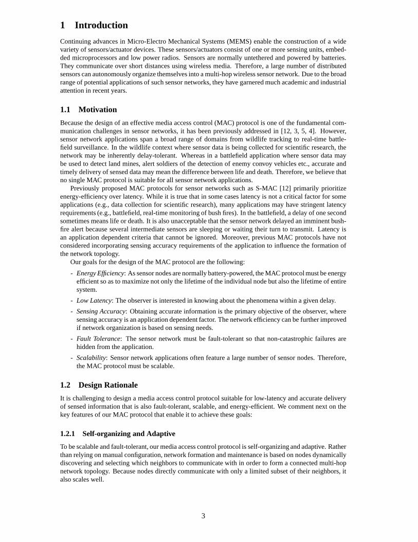
To prolong the lifetime of an individual node, we use Select Minimum Neighbor (SMN) algorithm tominimize the number of neighbors of a node and prohibit a node communicating directly with its furtheraway neighbors, even if they are within the radio range. As sensors are normally deployed in harshoutdoor environment, the path loss exponent for sensor ground-lying antenna, in 800-1000MHz band, isusually close to four [6]. This prompted us to ask a fundamental question in sensor network: Who is anode’s neighbor? Figure 1 shows three nodes that are randomly deployed in the sensing field. Is node C a

C

B

A

d2d3

d1

Figure 1: C is not selected as a neighbor of A

neighbor of node A? Remember radio propagation loss is directly proportional to the fourth exponent ofdistance. If the energy required for direct transmission from node A to node C is larger than the cumulativeenergy required for the multi-hop path from A to B to C, then node C is not selected as a neighbor of nodeA. Our SMN algorithm is based on this propagation loss analysis.

1.2.3 CDMA-Based

Because we use multi-hop instead of direct long-range communication for energy efficiency, we increasenetwork latency. To compensate for the latency sacrifice, we use CDMA spread spectrum approach toimprove latency performance. With CDMA, all nodes can transmit in the same frequency band simulta-neously. Channels are distinguished by pseudo noise code (PN code) rather than the time slot in TDMAand frequency band in FDMA.

Simple FDMA approach can not be used because it is very difficult for a node to decide when tosynchronize to which frequency. With TDMA, each node must wait for its turn (time slot) to transmit.TDMA also requires stringent time synchronization between a node and its neighbors. Comparatively,CDMA requires less stringent timing issues versus TDMA. CSMA is suitable for low traffic (less collision)scenarios as the media is shared by all sensor nodes. Because sensors are most likely to transmit datasimultaneously when an event occurs, CSMA is not a good choice with its backoff transmission approach.Collided packets must be discarded and energy is wasted. CSMA also suffers from hidden terminalproblem. Use of RTS, CTS and ACK control packets in CSMA causes significant overheads for shortsensor data packets.

4

By employing CDMA technique, our MAC protocol design is contentionless and the communicationsare peer to peer. Each node can transmit to its neighbors without using any control packet exchangesuch as IEEE 802.11 RTS, CTS, ACK, etc. Although these control packets are small, the data packetsin sensor networks are also small. Elimination of these control packets exchange will reduce the radioenergy consumption significantly.

Because CDMA increases the energy expended by the coding and decoding electronics, our protocolmust be based on low power CDMA modem technology. Chien et al [8] designed a low-power DSSS(Directed Sequence Spread Spectrum) modem architecture on an FPGA prototype that shows a powerdissipation of 33mW. When implemented using CMOS ASIC technology, the estimated power is lessthan 1mW. We believe with the advances in technology, the electronic power consumption will continueto decrease, and the ratio between the electronic power consumption and the radio amplifier power con-sumption will also decrease because the radio signal power is more distance dependent and less technologydependent.

Organization — The rest of this paper is organized as follows. Section 2 describes related work.Section 3 presents the technical background necessary for understanding our protocol design. Section 4elaborates the protocol design and network formation process. Section 5 provides simulations and analy-sis. Section 6 discusses several further improvements and research directions. We conclude our paper inSection 7.

2 Related Work

Media access control protocols for ad hoc sensor networks have been previously addressed [12, 3, 5, 4].These protocols can be broadly classified into contentionless and contention-oriented. ContentionlessMAC protocols for sensor networks are based on Frequency Division Multiple Access (FDMA) or TimeDivision Multiple Access (TDMA) approaches. Contention-oriented MAC protocols are adapted from theIEEE 802.11 standard.

SMACS (Self-Organizing Media Access Control for Sensor Networks) [5] is a distributed protocolwhich enables a collection of nodes to discover their neighbors and establish transmission/receptionschedules for communicating with them without the need for any local or global master nodes. Eachnode maintains a TDMA-like frame called superframe, in which the node schedules different time slots tocommunicate with its known neighbors. In SMACS, neighbor discovery and channel assignment phasesare combined so that by the time nodes hear from all their neighbors, they would have formed a connectednetwork. Although network wide time synchronization is not necessary, the communicating neighbors ina subnet still need to be time-synchronized. Power conservation is achieved by turning off the radio duringidle time slots. Unlike our protocol, network formation in SMACS is not location-aware. A node mayselect a neighbor that is further away from it instead of a near by neighbor. Because radio propagationloss is directly proportional to the fourth exponent of distance, it is not energy-efficient. Moreover, ifthe TDMA time slots of two neighbor nodes do not overlap, these two nodes will disengage from eachother. By using a TDMA approach, a node must wait its turn to transmit to a specific neighbor even if thechannel is idle. And this waiting time can accumulate along the multi-hop route from source to sink.

Woo and Culler [4] proposed a CSMA-based MAC protocol, designed especially to support the peri-odic and highly correlated traffic of some sensor network applications. They propose an adaptive trans-mission rate control (ARC) scheme, whose main goal is to achieve media access fairness by balancing therates of originating and route-through traffic. Because it is CSMA-based, this approach may suffer fromcontrol overheads and hidden terminal problems.

Shih et al[3] investigate the impact of non-ideal physical layer electronics on MAC protocol designfor sensor networks and proposed a centrally controlled MAC scheme. While a pure TDMA schemededicates the full bandwidth to a single sensor node, a pure FDMA scheme allocates minimum signalbandwidth per node. Pure TDMA is not always preferred due to the associated time synchronization cost.The hybrid TDMA/FDMA scheme they propose optimizes the power consumption of the transceiver andresults in lowering the overall power consumption of the system.

Inspired by PAMAS [9], SMAC (Sensor-MAC) [12] is based on IEEE 802.11 standard but improvesthe energy inefficiency of 802.11. SMAC identified several major sources of energy waste includingcollision, overhearing, control packet overhead, and idle listening. SMAC uses IEEE 802.11 CSMA/CAapproach to avoid collisions. To avoid overhearing, SMAC puts a node to sleep when a neighbor node istransmitting. A scheduled periodic sleep and listening pattern is used to decrease the idle listening energyconsumption. The main drawback of SMAC is high message delivery latency as SMAC is designed tosacrifice latency for energy savings. Actually, the assumption of SMAC design is that applications have

5

long idle periods and can tolerate latency in the order of network messaging time.LEACH (Low-Energy Adaptive Clustering Hierarchy) [10] is a cross-layer protocol design, encom-

passing MAC and network layers. It provides a combined TDMA/CDMA based MAC approach. Eachnode communicates with a dynamically elected cluster head directly (no multi-hop) using TDMA scheme.Cluster heads communicate with remote destination (sink) directly using a CDMA approach. In contrast,our MAC protocol relies exclusively on CDMA techniques to reduce overall network interference.

3 Background

This section presents the technical background for our protocol design, focusing on radio propagation andcode division multiple access (CDMA).

3.1 Radio Propagation

Neighbor selection for energy-efficient network formation in our MAC protocol is motivated by radiopropagation behavior. The mechanisms behind electromagnetic wave propagation are diverse, but cangenerally be attributed to reflection, diffraction, and scattering [19]. The free space propagation model isgiven by Friss equation as shown below:

��������� ��� ����� ������������ � � ��� (1)

where���

is the transmitted power,� � �����

is the received power which is a function of the transmitter-receiver (T-R) separation,

���is the transmitter antenna gain,

� �is the receiver antenna gain,

�is the T-R

separation distance in meters,�

is the system loss factor (�����

), and�

is the wavelength in meters.The above equation reveals that the radio propagation loss in free space is directly proportional to thesquare of distance. A single line-of-sight path between two sensors is seldom the only physical meansfor propagation. The two-ray ground reflection model considers both the direct path and a ground reflectpropagation path between transmitter and receiver. The received power at distance

�is predicted by

� � ������ ������� � � � �!��� � �"� � � ���# � (2)

where�$�

and� �

are the heights of transmit and receive antenna respectively. Above equation shows afaster power loss than free space equation 1. Sohrabi et al [6] have shown that for ground-lying antennas(which is normally the case for sensor nodes), in 800-1000 MHz frequency band, the average range ofpath loss exponent is between 2.2 to 5. This motivates that multi-hop communication should be usedinstead of direct communication between sensor nodes for energy efficiency.

The goal of our Select Minimum Neighbor (SMN) algorithm is to minimize the number of neighborsof a node and only allow a node to communicate directly with its limited neighbors only when there is noalternative multi-hop path that can provide a less energy consuming route. The SMN algorithm will bediscussed in Section 4.3.

3.2 Code Division Multiple Access

We use CDMA spread spectrum approach for the following reasons:

- With CDMA, all nodes can transmit in the same frequency bandwidth simultaneously.

- CDMA requires less stringent time synchronization compared to TDMA.1.

- CDMA is contentionless and therefore does not need RTS/CTS/ACK control packet exchange be-tween sensor nodes.

- Spreading spectrum implies the reduction of multi-path effects and good anti-jam performance.Data spreading results in greater immunity to radio frequency interference as compared to narrow-band signaling. And that is why IEEE 802.11b standard also employs DSSS (Direct SequenceSpread Spectrum) for better channel performance.

1CDMA does need synchronization of the locally generated code signal and received signal. This code synchronization is ac-complished at the receiver side.

6

- CDMA requires stringent power control, which is a positive feature for power saving purpose forsensors. The inherent static characteristic of sensor node makes the power control less complex thanCDMA cellular system.

- The generation of PN code is simple, several shift-registers are enough. The coded signal is simplymultiplication of base band signal and PN code with DS-CDMA.

- Because receiver use the same frequency to receive, the frequency synthesizer is simple.

- Coherent demodulation of spread spectrum signal is possible.

Although CDMA system increases the coding and decoding energy consumption, the spreading of base-band signals gives a much better channel relative to non-spreading signals. Spread spectrum (SS) systemcan use less transmission power to achieve the same bit-error-rate (BER) performance when compared toa non SS system.

3.2.1 Pseudo Noise Codes

CDMA uses pseudo-random noise code (PN code or PN sequence) to differentiate channels. A PN codeis a sequence of chips valued -1 and 1 (polar) or 0 and 1 (non-polar). Such bit-sequences have noise-likeproperties like spectral flatness and low cross and auto correlation values, and thus complicate jamming ordetection by non-target receivers [20]. In practice, the PN sequence selected must have both good cross-correlation and good auto-correlation because the receiver uses cross-correlation to separate the appro-priate signal from other interfering signals (those destined for other receivers), and uses auto-correlationto reject multi-path interference. Specific PN codes include Walsh codes, M-sequences, Gold codes andKasami codes. Codes can be orthogonal or non-orthogonal. Walsh code sets are orthogonal. They aregenerated by the Hadamard matrix expansion as shown below:

� ��� ����� � � �� � �� �

���� (3)

with the seed matrix

��� ��(4)

3.2.2 Processing Gain

The main parameter of a CDMA spread spectrum system is the processing gain, which is defined as theratio of spread data rate to the initial data rate:

� �� �

�� (5)

where � �is the transmission bandwidth, and �� is the bandwidth of the information (baseband) signal. For

example, IS-95 defines the original base band speech data rate of 9600 bps, after convolution coding (forFEC, forward error correction) and Walsh coding (spreading), the data rate is spreaded to 1.2288 Mbps.So the processing gain is

�� ����������������������� � !�"#���$� �%�&� � � � � . Processing gain determines thenumber of simultaneous transmissions that can be allowed in a system. CDMA signal experiences highlevels of interference as all other CDMA coded signals are treated as noise. The total interference alsoincludes background white noise and other spurious signals. When the signal is received, the correlatorsat the receiver use the processing gain to extract the desired signal out of the noise. For CDMA spreadspectrum systems it is advantageous to have a processing gain that is as high as possible to allow manysimultaneous transmissions. Fortunately, we are not expecting a sensor node to have as many neighborsas a CDMA cellular system.

Our Select Minimum Neighbor algorithm even minimizes the number of neighbors. A node onlycommunicates directly with its neighbors only when there is no other neighbor node that can providea multi-hop path with less energy consumption. This means that we may achieve similar channel char-acteristics (e.g., BER) with possibly lower processing gain. We will discuss Select Minimum Neighboralgorithm in Section 4.3.

7

3.2.3 Spread Spectrum Techniques

Different spread spectrum techniques exist: Direct-Sequence (DS), Frequency-Hopping (FH), Time-Hopping (TH) and Multi-Carrier CDMA (MC-CDMA). It is also possible to combine these techniques.

DS-CDMA is the most popular technique and easy to implement because the baseband signal is simplymultiplied with a PN sequence. The main problem with DS-CDMA is the so-called near-far problem.Suppose two nodes transmit with the same power, and the interfering transmitter is relatively much closerto the receiving node than the intended transmitter. In this case, the correlation in the receiver of thesignal received from the interfering transmitter may exceed that of the signal received from the intendedtransmitter (i.e., the correct code). As a result the intended data is hard to recover. The solution toovercoming the near-far problem is to use stringent power control so as to ensure that the received signalsalways have the same amount of power at the receiving node. Fortunately, sensor nodes are normallystatic instead of mobile, and the power control is much easier compared to the CDMA cellular systemwhere mobile stations are always moving. Furthermore, with our Turning Off Redundant Node and SelectMinimum Neighbor algorithms, we can achieve an evenly deployed sensor network such that a nodenormally does not have two neighbors that have very large difference in distance.

The disadvantage of FH-CDMA is that it hard to obtain a high processing gain compared to the DS-CDMA. FH-CDMA also require a very fast switching frequency synthesizer that is hard to build within asensor node.

Everything comes at a cost. The trade off of using CDMA spread spectrum approach is the increasedcomplexity design at the receiver side. CDMA uses multiple correlating receivers called rake receiver.The design of low power DSSS modem within a sensor node is an open research area [8].

4 The Protocol Design

In this section, we elaborate the network formation process in CSMAC. Our network formation processhas several phases as illustrated by Figure 2.

Nodes Startup

Time Sync

Location Broadcast TORN SMN Normal OperationChannel Setup

Figure 2: Network Formation Phases

We make the following assumptions in our protocol design:

- Each node starts up at almost same time.

- Nodes need not be synchronized at start up, but should be eventually synchronized before the be-ginning of location broadcast phase. The granularity of time synchronization required is low forour scheme (e.g., one second is enough). In this paper, we assume that each node in the networkcan be synchronized to a system clock. The timing reference can be provided by one or more GPSenabled nodes or use some technique such as the algorithm proposed by Lamport [15]. As CSMA isemployed during the network formation stage, the time frame of each phase should be long enoughto provide each node with an opportunity to transmit.

- We assume that each node can estimate its location. This location information can be relative to areference and does not need to be the absolute location. Sensors can also use either internal GPSreceiver or alternate location estimation approaches 2

4.1 Location Broadcast

In the location broadcast phase, each node uses a CSMA/CA based approach to broadcast its locationinformation to its radio range neighbors. As this is a broadcast, nodes cannot use RTS/CTS.

To reduce the probability of collision and make sure each node has an opportunity for a successfulbroadcast, we employ large contention window sizes and let each node transmit its location informationseveral times. By using CSMA/CA, we can not eliminate the hidden node problem shown in Figure 3.Because there is an obstacle between A and B, they can not detect each other. A and B may transmit at

2Please refer Bulusu [7] for a survey of location techniques for sensor networks.

8

A

B

C

D

Figure 3: Hidden Node Problem

the same time and the signals will collide at node C. Thus C can not record the location information of Aand B. As this is a broadcast and there is no negative acknowledgement message from C, both A and Bwill not become aware of the problem. But when C get the media to transmit, both A and B can hear themessage and record the location information of C in their memory. We will show how this hidden nodeproblem can be resolved during the TORN and Channel Setup phases later.

At the end of the location broadcast phase, each node should have a list with the locations of its radiorange neighbors. We call this list Redundant Neighbor List (RNL). We now describe the TORN and SMNalgorithms and then we discuss the channel allocation and network formation process. The backup processof inactive nodes will be presented last.

4.2 Turning Off Redundant Node (TORN)

Once a node has an RNL, it ranks all its neighbors according to the distance between itself and a neighbor.Before deciding who should be selected as its neighbor, the node first decides if there are any neighborswithin its redundant range. If sensor nodes are deployed with high redundancy, the probability of havingneighbors within redundant range is high.

We denote the sensing resolution as ��� (e.g., two meters). Any node within the circle with radius of��� will be treated as a redundant node. We assume redundancy relationship between two (or more) nodesis symmetric, e.g., if node A thinks node B is in its redundant range, node B also thinks node A is in itsredundant range.

Similarly, each node uses a CSMA/CA based approach to negotiate who should keep active and whoshould turn off. By doing this, a random timer is used to avoid collisions. The first node that get the mediato transmit can inform its redundant neighbor(s) to turn off by including the ID numbers of these nodes.When a node receives a message asking it to turn off, it will record the ID number of the node issuing theturn off request. It then converts to be a backup node to the issuing node. At the same time, other nodesthat receive the turn off message will remove the entries of those nodes requested to turn off.

For a node requested to turn off, it keeps alive until it gets the receiving frequency (more about thislater) of the node it is backing up until the Channel Setup phase. The inactive node then goes to sleep andwakes up only after some period of time to check the energy level of the active node and decide whetherit should take over the responsibility of the active node. We discuss backup process in subsection 4.5.

An example is given in Figure 4. We assume the radio range to be such that each node can reach everyother node within this small area. Suppose node B is within the sensing resolution (SR) range of nodeA and B is also within the SR range of node C. Note both A and C are within the SR range of node B.Suppose they have RNL as follows (the redundant nodes are in bold italic font):

- A RNL: B, C, D, M, H, E, O, . . .

- B RNL: A, C, D, H, G, E, M, . . .

- C RNL: B, H, A, E, G, F, D, . . .

If node A grabs the media to transmit first, it will transmit a turn off message including the ID number ofnode B. When node B receives this message, it turns itself into a backup node to node A and broadcaststhat it will become an inactive node. When node C receives this turning off message from A to B or thebroadcast message of B, C knows that B will become an inactive node and C will remove node B from itsRNL. If node B gets the media to transmit before A and C, it will transmit a turn off message includingthe ID numbers of both node A and node C. Node B can randomly select one node as its primary backupnode and the other as second. When other nodes receive this turning off message (such as D, H, etc.), theywill remove both A and B from their RNL. If we do not want a node to have too many backups, we canset the expire timer of a node based on the number of redundant neighbors. For example,

Timer = (Random delay) + (Constant delay) *(Number of redundant neighbors - 1)

9

If we set the Constant delay to be larger than the contention window size, a node that has moreredundant neighbors will be less likely to become an active node during TORN phase. We do this toprovide fairness. For example, if B becomes the active node, both A and C will turn off. While B has twobackups, M, D, E, and H do not have even one.

B C

D

E

G

H

J

K

O

N

M

L

A

P

Q

R

F

I

Figure 4: A TORN Example

The goal of TORN is to preserve the energy of redundant nodes for future use and prolong the lifetimeof the whole sensor network. In practical deployment, we can bundle two (or more) sensors together (ifthe deployment can not be planned) or deliberately put two (or more) sensors within the SR range (if thedeployment can be planned), our TORN algorithm will turn one (or more) redundant nodes into inactivenodes. These inactive nodes only turn on when those active nodes are near depletion of their energy orphysically damaged.

At the end of TORN phase, only active nodes are left in the network. The resulting neighbor list ineach active node is called non-redundant neighbor list (NNL). This NNL will be used in the SMN process,which we discuss in the next subsection.

Hidden Node Problem: Consider Figure 3. Assume B is within the SR range of C, but C does notknow B’s location. So C thinks it does not have a redundant neighbor and keeps silent during the TORNphase. But because B has the location information of C, it knows that C is its redundant node. WhenB grabs the media, it sends an RTS request including C’s ID number and its own ID number. When Creceives this RTS message, it replies with a CTS message including the ID numbers of both B and C. Bthen sends a turn off request to C with its (B) location information. C then knows that it has a redundantneighbor B, and perhaps due to a hidden node problem or collision, it did not record B’s location in itsRNL at location broadcast phase. C broadcasts a sleep message to inform its neighbors that it will becomean inactive node. When A receives this message, it removes C from its RNL.

4.3 Select Minimum Neighbor (SMN)

After the TORN stage, each active node has a list (NNL) of location information of its radio range neigh-bors. A node will not select all of them as neighbors. It only selects a node as its neighbor if there isno other neighbor that can provide a multi-hop path with lower power consumption. We designed analgorithm for a sensor node (we call it seed node) to select its neighbors. With the list (NNL) of activeneighbors, the seed node ranks them according to their distances to the seed. Then starting from the lastnode (furthermost) in NNL, each node will be tested against other neighbors in the NNL based on a spe-cific radio propagation model (e.g., two-ray ground) and an electronic energy dissipation model. If anyneighbors in the NNL can provide a multi-hop path from seed to the current tested node with less powerconsumption, the current tested node will not be selected as a neighbor and will be removed from NNL.The algorithm is shown below:

Select Minimum Neighbor Algorithm:

INPUT: A list of neighbor nodes with its locationinformation (ranked according to distanceto seed node)

OUPUT: A list contains minimum number of neighbors

BEGIN:VECTOR INPUT = List of neighbor nodesVECTOR OUTPUT = NULL;

10

NODE SEED = seed node;NODE CURRENT = NULL;NODE TEMP = NULL;BOOLEAN isNeighbor = TRUE;DOUBLE p1, p2, p3; // Transmission powerDOUBLE Tx_elec; // Tx electronic power consumptionDOUBLE Rx_elec; // Rx electronic power consumption

LOOP1:CURRENT = last node in INPUT vector;p1 = Tx power required from SEED to CURRENT;isNeighbor = TRUE;

IF (INPUT IS NOT NULL)LOOP2:TEMP = next node in INPUT;p2 = Tx power required from SEED to TEMP;p3 = Tx power required from TEMP to CURRENT;IF (p1 > p2 + p3 + Tx_elec + Rx_elec)THEN { isNeighbor = FALSE; BREAK LOOP2; }

END OF LOOP2

IF (isNeighbor IS TRUE)THEN {Add CURRENT to OUTPUT vector;}REMOVE CURRENT from INPUT vector;END OF LOOP1

RETURN OUTPUT;END

After the SMN phase, each active node only has a minimum set of neighbors and we call the resultingneighbor list minimum neighbor list (MNL). This MNL will be used in the Channel Setup process whereina peer-to-peer communication channel will be setup for each neighbor in MNL and the seed.

By using TORN and SMN, we want to achieve an evenly deployed sensor network that is energy-efficient without sacrificing the sensing accuracy. Figure 5 shows the point of view of an active sensornode after the TORN and SMN phases. � �

denotes the sensing resolution range and � � denotes the radiotransmission range. Node A has one redundant node and only selects five nodes as its neighbors althoughits radio can reach more nodes.

R2

R1

A

Figure 5: An Active Node’s Point of View after TORN and SMN phases.

4.4 Channel Allocation and Network Formation

At the end of SMN phase, each node only has minimum set of neighbors. The last step is to allow eachnode to setup connections to all it neighbors in the MNL.

4.4.1 Channel Allocation Pattern

Before we discuss the channel allocation process, we first specify the channel allocation pattern. If weneed to use orthogonal PN codes, we only have limited codes available. Assume we use 128 chip/bit

11

Walsh code sets, we only have� �&�

codes available instead of� � ���

. This will cause interference problemsif all nodes use the same frequency. As shown in Figure 6 (a), which illustrates A and B negotiating to usePN1 for communication from A to B. We can avoid both node A and node B using PN1 again with theirneighbors but we can not avoid node C and node D using the same code. The conditional probability of thisscenario is

� � ������ ��� � �� �� � ��� � � � � � �� � ��� � � ������ ��� � � � � � �� � ��� � � � ��� �&�

, which is not very low. Even if we use stringent power control, the interference may stillexist. We propose two approaches to resolve this problem, namely using spatial diversity andfrequency diversity.

By spatial diversity, we separate nodes using the same PN code spatially. We make eachnode negotiate with its neighbors using full transmission power so that each radio range neighborcan hear these messages. If node C and node D are within the radio range of node A or nodeB, C and D can hear the negotiations between A and B. Thus they know that PN1 was usedby other nodes located within their radio range. This way node C and node D will not selectPN1 for communication. When the network enters normal operation phase, each node will nolonger transmit at full power but only communicate with its minimum neighbor with much lowercalibrated transmission power.

A problem with this approach is that if the radio range can cover more than 64 (128 PN codescan only serve 64 node pairs) nodes, some nodes may not be able to get a PN code to use. Thisapproach has direct relation to the density of sensor network. The density can range from fewsensor nodes to hundred sensor nodes in a region, which can be less than 10m in diameter. Thedensity � is calculated as [7]:

�� ��������� ���� (6)

where�

is the scattered sensor nodes in region�

, and R is the radio transmission range. Gener-ally, �� ���� gives the number of nodes within the transmission radius of each node in region

�. To

make this approach functional, the density � must be less than half the available PN codes. Twomajor problems with this approach are: 1) Tx and Rx can not happen simultaneously becausethe transmitter power is so high that it will drown out any receive messages, 2) CDMA near-farproblem.

A B C DPN2

PN1 PN3

PN4

PN1

PN5

(a)

f1 f2 f3 f4

A

PN1

PN2

PN3

PN4

PN1

PN5

(b)B C D

Figure 6: Channel Allocation Patterns

In frequency diversity approach, we use FDMA plus CDMA as shown in Figure 6 (b). Eachnode uses a different frequency band to receive signals. As bandwidth is not a scare resource insensor networks, this may be a practical approach. For example, assume the sensor base bandsignal is 10Kbps and we use 128 chip/bit. The spreading bandwidth is 1.28MHz. If we use902-928 Industry, Scientific, and Medical (ISM) band, we can have about 20 frequency bands.This will give us �����! "�$#��%��&�'$# channels! If we use a higher frequency spectrum, such as2-3GHz, we can have more frequency channels. The probability of two nodes selecting both thesame frequency band and the same PN code is very low. By using frequency diversity, both theTx and Rx can happen simultaneously and the interference caused by competing transmissionsat a specific receiving node are also reduced.

In CDMA, all received signals are noises except the intended signal if the same frequency isused. Once this noise floor reaches a certain level, the intended signal is unable to be retrieved. If

12

the receiver of each node can use a different receiving frequency, those transmission signals fromnon-neighbors will not be able to penetrate the band pass filter at the front-end of the receiver.Thus those signals will not contribute to the noise floor. Assume a sensor node is receiving froma neighbor, those nodes that may contribute to the noise floor are the ones listed in its MNL.And those noise, if existed, are normally expected signals from its other neighbors. The problemwith this approach is that the transmitter is required to synthesized to different frequencies fortransmission to different neighbors and thus this approach is not suitable for broadcast (we arecurrently designing a more efficient broadcasting scheme with frequency diversity). We adoptedfrequency diversity in our design and simulation because of its better latency performance versusspatial diversity. We plan to incorporate spatial diversity in future research because it has betterbroadcast performance and simpler transceiver design, especially when ultra-wide-band (UWB)technology becomes available for sensor networks.

4.4.2 Channel Allocation Process

We now describe the channel allocation process. At this stage, each node no longer transmits atfull power. Each node estimates the transmission power required to reach its furthermost neigh-bor in its MNL and uses this power level for the negotiation process. This allows other nodesthat are far enough from this node to initiate another setup process simultaneously. Similarly,CSMA/CA is used by nodes to setup connections with each other. When a node grabs the media,it will hold the media until it finishes the channel allocation with all of its neighbors in the MNL.

Figure 4 illustrates this process. At the beginning of Channel Setup phase, each node sets arandom timer and begins to count down.

1. Assume node A’s random timer expires first, A sends a Request-to-Send (RTS) packet toits first neighbor in the MNL, in this case, C.

2. If C is not in another channel setup process with one of its other neighbors, say G, C willrespond with a Clear-to-Send (CTS) packet. Otherwise, C will not respond the request ofnode A.

3. If A does not receive the CTS packet from C in time, A knows that C is busy with anotherchannel setup process and will back-off its initiation. Other nodes that receive the RTS orCTS packet will hold active initiation for channel setup and only passively reply if needed.

4. Suppose C is not in another channel setup process, when A receives the CTS packet fromC, A will initiate a channel setup packet to C. We call this packet SYN packet. There aretwo possible cases for A:

(a) A is not connected with any other neighbor (in this case, the receiving frequency of Ais not fixed) and,

(b) A is connected with some other neighbors (in this case, the receiving frequency of Ais fixed).

In the first case, A will randomly select a frequency band as its receiving frequency and arandom PN code as its transmission PN code to node C. In the second case, the receivingfrequency of A is fixed and it only randomly selects a PN code to node C. A must guaranteethat this PN code has no conflict with PN codes employed by A for communicating with itsother neighbors. A then encapsulates its receiving frequency, a flag to indicate whether thisreceiving frequency is fixed, its transmitting PN code to C, and the ID number of A and Cinto a SYN packet and transmit to C.

5. When C receives this SYN packet, it will reply with a SYNACK or SYNNAK packet.There are also two possible cases for node C:

(a) C is not connected with any other neighbors (In this case, the receiving frequency of Cis not fixed) and,

13

(b) C is already connected with some other neighbors (In this case, the receiving frequencyof C is fixed).

In the first case, C will select a random receiving frequency and a random transmissionPN code that differs from the receiving frequency and PN code of A. In the second case,C first checks if there is any conflict of the transmission PN code and receiving frequencyof A (If receiving frequency flag of A is not set) with its own receiving frequency andthe PN codes employed with its other neighbors. If any conflict occurs, C will reply witha negative acknowledgment packet (SYNNAK) indicating that the transmission PN codeor receiving frequency of A is invalid. C then randomly selects its receiving frequencyand transmission PN code in the first case and only randomly select a transmission PNcode in the second case. The PN code selected by C must meet following criteria: 1)no conflict with the PN codes that it employed with its other neighbors, 2) if C and Ahappen to employ the same receiving frequency and both their receiving frequencies arefixed (this may happen when both A and C are attached to other neighbors before theirown channel setup process although this probability is low), C must guarantee that the PNcodes employed are different. C then encapsulates its validation of the transmission PNcode and receiving frequency of A, its own receiving frequency, a flag to indicate whetherits receiving frequency is fixed, its transmitting PN code to A, and the ID number of C andA into a SYNACK packet and transmits to A.

6. When A receives the SYNACK (or SYNNAK) packet from C, it first checks whether theacknowledgement is positive or negative. If the acknowledgement is negative, A will re-select the PN code or receiving frequency (if not fixed) and initiate a new SYN packet toC. If the acknowledgment is positive, A uses a similar validation process to validate thetransmission PN code and the receiving frequency of C. If any conflict occurs, A will replywith a negative acknowledgment (NAK) to C.

7. When C receives a NAK packet, C will re-select its PN code or receiving frequency andreply with a new SYNACK packet to A.

8. If no conflict occurs, A will reply with a positive acknowledgment (ACK) packet to C.

9. When C receives this ACK packet, it knows that the PN code and receiving frequencyallocation has succeeded.

10. After this, A and C may calculate the required transmission power to each other based onthe distance and possible channel characteristics (e.g., SNR, BER, RSSI, etc.). A and Cthen synthesize their receivers to their respective receiving frequencies and conduct a pilotrun that should be initiated by A. A and C may exchange several small packets to setuptheir transmission power to the correct level. When the pilot run finishes, the channel setupbetween A and C is finished. A and C then synthesize back to CSMA mode for furtherconnection setup process. A will repeat this process until it finishes the connections withall of its other neighbors. After that, A will broadcast a clear packet indicating that itfinished the connection setup and the media is now released. When other nodes receive aclear packet, they can initiate connection setup process with their neighbors if needed.

The packets exchanged between nodes during the connection setup are:

- RTS/CTS/Clear, control packets used to access the media;

- SYN, sent by the active node to initiate a channel setup process;

- SYNACK/SYNNAK, response to SYN packet, send by the passive node that is required tostart a channel setup process;

- ACK/NAK, acknowledgment to the SYNACK packet, either positive or negative.

Figure 7 shows three different scenarios in the channel setup process. where (a) represents thenormal operation, (b) shows the failed validation of PN code or receiving frequency of A, and(c) shows the failed validation of PN code or receiving frequency of C. After the channel setupphase, each node has the listed information stored in its memory:

14

A C A C A C

SYN

CTS

RTS

SYNNAK

SYN

SYNACK

ACK

RTS

CTS

SYN

SYNACK

ACK

RTS

CTS

SYN

SYNACK

NAK

SYNACK

ACK

(c)(b)(a)

Figure 7: (a) Normal Operation. (b) C disagrees with the PN code or Receiving Frequency of A. (c) Adisagrees with the PN code or Receiving Frequency of C.

Node Information:Rx Frequency -- the receiving frequency

of this node

Each Neighbor Information:ID -- the neighbor identity numberRx PN code -- from neighbor to this nodeTx PN code -- from this node to neighborTx frequency -- the receiving frequency

of neighborTx power level -- transmission power level

from this node to neighbor

4.5 Backup Process

In this subsection, we provide a brief description about the backup process (as we are workingon a detailed backup process at this stage). After the channel setup phase, an inactive nodeturns off completely and wakes up after some period of time. The inactive node then checks theenergy level of the active node that it is backing up and decides whether it should take over theresponsibilities of the active node. The checking period is based on the energy level of the activenode. E.g., at the beginning of the deployment of sensor network, the active node has full energylevel, the checking period can be long, such as once a day. When the energy level of the activenode drops to a certain level, the checking period should be decreased, such as once an hour.When the energy of the active node is near depletion, the backup node and active node negotiatewith each other and transfer the responsibility to the backup node.

4.6 Summary

We described a novel CDMA-based, self-organizing, location-aware MAC protocol for ad hocwireless sensor networks. Our network formation process comprises of several phases includingLocation Broadcast, Turn off Redundant Node (TORN), Select Minimum neighbor (SMN), Chan-nel Setup, and Normal Operation. The TORN scheme is employed to preserve the energies ofredundant nodes for future use while still keep sufficient sensing accuracy. The SMN algorithmis employed by a sensor node to select a minimal subset of communicating neighbors to conserveenergy. CDMA approach is used for efficient low latency performance by allowing simultaneoustransmissions.

We have not designed a sleep and wakeup scheme at this stage. Part of the reasons is that weare targeting the applications that have higher traffic and stringent latency requirements. Morediscussions about sleep and wakeup are presented in 6.4.

15

5 Simulations and Analysis

We implemented and simulated our protocol in Network Simulator (NS-2). All phases exceptTurning off Redundant Nodes (TORN) have been finished so far. These phases include locationbroadcast, select minimum neighbor (SMN), channel setup, and normal operation. DSSS (Di-rected Sequence Spread Spectrum) is simulated as a PN code attribute in packet header. Whenthe packet is received at a receiving node, this PN code is checked against PN codes the receiv-ing node is monitoring. If a match is found, the packet is passed to the next step for furtherprocessing. If no match is found, the packet is discarded. This procedure is used to simulate thede-spreading process. In this simulation, we call our protocol CSMAC (denote CDMA SensorMAC).

The goals of this simulation are to measure the energy efficiency and latency trade-offs inCSMAC. The idle energy consumption is not traced at this stage (the idle energy consumptionand sleep mode is further discussed in 6.4). Also, the energy consumed at the setup phase ofCSMAC is not traced. As a comparison, we also measured the performance of SMAC [12] asSMAC was also implemented in NS-2.

SMAC is similar to IEEE 802.11 but uses a periodic sleep to save idle energy consumptionand turns off nodes during data transmission by neighbors to save the energy consumed in over-hearing.

We adopted a simple energy dissipation model that is used in LEACH [11]. The modelis shown in Figure 8. This model separates the electronic energy consumption and amplifier

d

ElectronicTransmit

ElectronicReceiveTx Amplifier

k bit packet k bit packet

Figure 8: Radio energy dissipation model

energy consumption at the transmitter side. For comparison purposes, we used the same physicalparameters for both CSMAC and SMAC.

Data Rate: 10KbpsPropagation Model: TwoRayGroundAntenna Height: 0.1 meterAntenna Gain: 1System Loss: lRx Threshold: 1nWCarrier Sense Threshold: 0.1nWRx Elec Power: 20mWTx Elec Power: 20mWFull Radio Signal Power: 200mWISM Frequency Band: 902-928 MHz

More detailed physical parameters are not implemented at this stage. For example, the effi-ciency of the amplifier in general, is only about 30 � 40%. CDMA consumes more energy for itscoding and decoding. But on the contrary, CDMA provides a better channel, and as a result, canuse lower transmission power to achieve the same bit-error-rate (BER) performance. We plan toimplement these in our future simulations.

We use two simple topologies that were used by SMAC to do the measurements.

5.1 Measurement with Two-Hop Network Topology

CSMAC uses contentionless approach and the communications are peer-to-peer. Broadcastingmeans multi-unicast dependent on the number of neighbors (a more efficient broadcast imple-mentation is still under progress). This means CSMAC is not efficient with broadcast traffic but

16

on the contrary, is efficient with unicast traffic. We tested both (i) the pure broadcast traffic and(ii) the combined broadcast and unicast traffic with a simple topology shown in figure 9. The

1

3

Source 1

0Source 2

2

Sink 1

4

Sink 2

Figure 9: Two-hop network with two pairs of sources and sinks

routing protocol used in this simulation is DSDV (Destination Sequence Distance Vector) andapplication used is CBR (Constant Bit Rate) traffic. The radio signal power is set to 20mW. Thedistances between nodes are deliberately set to make sure nodes 0, 1, 3 can hear each other andnodes 2, 1, 4 can hear each other.

To test pure broadcast traffic, we simply did not generate the application traffic. DSDVrouting protocol uses broadcast to exchange routing information periodically with its neighbors.Figure 10 shows the average node energy consumption with pure broadcast traffic. The figureshows that CSMAC consumes 50% higher mean energy per node than SMAC. We then tested a

120 140 160 180 200 220 240 2600

20

40

60

80

100

120

140

160

180

200Average node energy consumption for broadcast

Time (s)

Ave

rage

nod

e en

ergy

con

sum

ptio

n (m

J)

CSMACSMAC

Figure 10: Average per node energy consumption for broadcast traffic

scenario with combined broadcast and unicast traffic. Two sources and two sinks are used. TheCBR traffic interval is set to 5 seconds. Figure 11 shows the average node energy consumptionwith combined broadcast and unicast traffic. Surprisingly, CSMAC consumes 27% less meanenergy per node because the CBR traffic (unicast) contributes to the major part of the energyconsumed. CSMAC also eliminates RTS, CTS, and ACK packet exchange that are essentials inSMAC. In addition, CSMAC achieves a 62% lower mean packet latency as shown in Figures 12and 13. In most cases, the latency using CSMAC is simply the accumulation of the multi-hop transmission time. The first packet latency is much higher than the others because at thebeginning, each node has to use ARP (Address Resolution Protocol) to resolve the MAC addressof next hop before it can forward the data packet. Following packets do not need ARP anymore.This is the same for both CSMAC and SMAC.

We also tested this topology with directed diffusion routing protocol. Directed diffusion is arouting protocol especially suitable for distributed sensor networks. Directed diffusion was im-plemented in NS-2 and a ping application is provided for testing purposes (for more information,please refer to NS-2 manual).

We used two different ping senders and ping receivers to simulate two sinks and two sources.The measurement time is from 131s to 851s. Totally 73 ping messages have been sent between

17

100 200 300 400 500 600 7000

200

400

600

800

1000

1200

1400

1600Average node energy consumption for unicast and broadcast traffic

Time (s)

Ave

rage

nod

e en

ergy

con

sum

ptio

n (m

J)

CSMACSMAC

Figure 11: Average per node energy consumption for both unicast and broadcast traffic

0 10 20 30 40 50 60 70 80 90 1000

200

400

600

800

1000

1200

1400Packet latency from node 0 to node 2

Packet number #

Late

ncy

(ms)

CSMACSMAC

Figure 12: Packet latency from node 0 to node 2

0 10 20 30 40 50 60 70 80 90 1000

200

400

600

800

1000

1200

1400Packet latency from node 3 to node 4

Packet number #

Late

ncy

(ms)

CSMACSMAC

Figure 13: Packet latency from node 3 to node 4

a source and sink pair. The ping message interval is set to 10 seconds. Figures 14 shows thatCSMAC consumes 34% lower mean energy per node compared to SMAC. Figures 15 and 16show the latency performance. CSMAC shows 59% lower mean message latency from node 0 tonode 2 and 72% lower mean message latency from node 3 to node 4 compares to SMAC.

18

100 200 300 400 500 600 700 800 9000

200

400

600

800

1000

1200

1400

1600

1800Average node energy consumption with directed diffusion traffic

Time (s)

Ave

rage

nod

e en

ergy

con

sum

ptio

n (m

J)

CSMACSMAC

Figure 14: Average node energy consumption with directed diffusion traffic

0 10 20 30 40 50 60 700

500

1000

1500Ping message latency from node 0 to node 2

Message number #

Late

ncy

(ms)

CSMACSMAC

Figure 15: Ping message latency from node 0 to node 2

0 10 20 30 40 50 60 700

500

1000

1500

2000

2500Ping message latency from node 3 to node 4

Message number #

Late

ncy

(ms)

CSMACSMAC

Figure 16: Ping message latency from node 3 to node 4

5.2 Measurement with Ten-Hop Network Topology

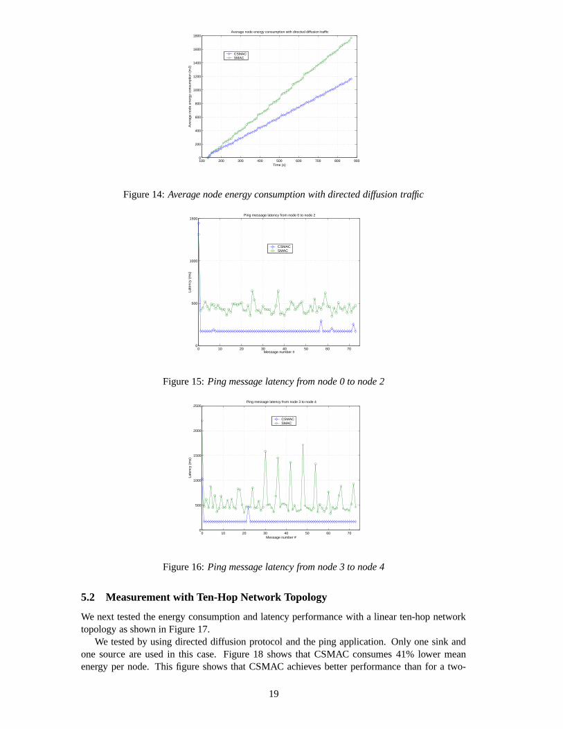
We next tested the energy consumption and latency performance with a linear ten-hop networktopology as shown in Figure 17.

We tested by using directed diffusion protocol and the ping application. Only one sink andone source are used in this case. Figure 18 shows that CSMAC consumes 41% lower meanenergy per node. This figure shows that CSMAC achieves better performance than for a two-

19

8 90 1 2 10

Source Sink

Figure 17: Ten-hop network with one source and one sink

hop topology because broadcast traffic is not severe in this linear topology. To simulate theCDMA may consume more power because of encoding and decoding process, we increase the

100 200 300 400 500 600 700 800 900 1000 11000

200

400

600

800

1000

1200

1400Average node energy consumption for 10 hop

Time (s)

Ave

rage

nod

e en

ereg

y co

nsum

ptio

n (m

J)

CSMACSMAC

Figure 18: Average node energy consumption for 10 hops

electronic power consumption to 40mW (both Rx and Tx). After this increase, CSMAC achievesthe similar average node energy consumption versus SMAC. This means that if the electronicenergy consumption for CDMA codec can achieve less than two times of normal non-CDMAelectronics, we can achieve the similar energy consumption in this linear topology (do not forgetthat CDMA can provide a much better channel!). But CSMAC achieves 74% lower mean latencyas shown in Figure 19.

0 1 2 3 4 5 6 7 8 9 10 110

0.5

1

1.5

2

2.5

3

3.5Average message latency

Number of hops

Ave

rage

Lat

ency

(s)

CSMACSMAC

Figure 19: Average message latency for 10 hops

5.3 Measurement of SMN with Random Topology

In this subsection, we tested our select minimum neighbor (SMN) algorithm with 20 randomlydeployed sensor nodes in a 50m 50m area. The initial radio signal power is set to 200mW,which equals the full radio signal power. This is to ensure that each node can reach all itsneighbors within its radio range. After the channel setup phase, the radio power is recalculatedaccording to the distance a node is from its neighbor.

20

Figure 20 shows the node connection pattern before SMN and Figure 21 shows the node con-nection pattern after SMN. From the diagrams we can see that after SMN, some nodes removedpart of ther neighbors to conserve energy. For example, nodes 6 and 8 are neighbors before SMNbut are not neighbors after SMN. This is the same for nodes 6 and 4, nodes 2 and 18, nodes 7and 19, nodes 10 and 14, etc.

0 5 10 15 20 25 30 35 40 45 500

5

10

15

20

25

30

35

40

45

50Connection pattern before SMN

X (m)

Y (

m)

15

0

19

13

7

10

12 14

3 11

4

186

2

8

5

16

9

1

17

Figure 20: Node connection pattern before using SMN

0 5 10 15 20 25 30 35 40 45 500

5

10

15

20

25

30

35

40

45

50

X (m)

Y (

m)

Connection pattern after SMN

15

0

19

13

7

10

12 14

3 11

4

18

6

2

8

5

16

9

1

17

Figure 21: Node connection pattern after using SMN

We tested the energy consumption and latency by using two pairs of sources and sinks withdirected diffusion ping application. One pair of source and sink is put on node 15 and node 0, theother is put on node 8 and node 10. The simulation time is from 241s to 551s. The ping messageinterval is 10 seconds. Totally 31 ping messages have been received at each sink.

Figure 22 shows the comparison of energy consumption with and without SMN. The diagramshows that 21% less mean energy is consumed with SMN. Figures 23 and 24 show the messagelatency comparison. From the diagram we can see that the latency from node 15 to node 0 doesnot have much difference. This is because the minimum number of hops from node 15 to node0 did not change after SMN. But for the message latency from node 8 to node 10, non-SMNachieves the better latency performance because non-SMN topology can provide a route withless number of hops compared to SMN topology. This reveals the trade-offs between the energyconsumption and latency performance.

21

200 250 300 350 400 450 500 550 6000

0.5

1

1.5

2

2.5Comparison of average node energy consumption with and without SMN

Time (s)

Ave

rage

nod

e en

ergy

con

sum

ptio

n (J

)

With SMNWithout SMN

Figure 22: Comparison of average energy consumption with and without SMN

0 5 10 15 20 25 300.4

0.6

0.8

1

1.2

1.4

1.6

1.8

2

2.2

2.4Comparison of ping message latency with and witout SMN

Message number #

Late

ncy

(s)

With SMNWithout SMN

Figure 23: Comparison of message latency with and without SMN from node 15 to node 0

0 5 10 15 20 25 300

1

2

3

4

5

6

7Comparison of ping message latency with and witout SMN

Message number #

Late

ncy

(s)

With SMNWithout SMN

Figure 24: Comparison of message latency with and without SMN from node 8 to node 10

6 Future Research

In this section, we comment on further improvements to our protocol. We are currently workingon some of them.

22

6.1 Broadcasting with Frequency Diversity

Broadcasting in our current design is implemented by multiple unicast to all neighbors, whichis not energy-efficient. An improved broadcast implementation is to employ two receivers in asensor node. One receiver synthesizes to a dedicated frequency band and is used for broadcasttraffic. This dedicated frequency band is common across all sensor nodes. A dedicated PN codecan be allocated by a sensor node for its broadcast data to all its neighbors. The detailed schemeis still under design.

6.2 Ultra-Wide-Band (UWB) with Spatial Diversity

We mentioned in section 4.4 that ultra-wide-band (UWB) is an attractive candidate techniquefor sensor networks. UWB employs baseband transmission and thus requires no intermediateor radio carrier frequencies. UWB has several advantages such as resilience to multi-path, lowtransmission power, and simple transceiver circuitry design. In general, UWB uses pulse positionmodulation (PPM). Because UWB employs baseband transmission without carrier frequencies,the frequency diversity we proposed in Section 4.4 can not be used and spatial diversity is thechoice with UWB. We believe this is an interesting and attractive direction and worth exhaustiveresearch efforts.

6.3 SMN Improvements

The SMN algorithm we described in Section 4.3 is only based on a specific radio propagationmodel (e.g. two-ray ground), which is not enough to reflect the real characteristics of a channel.In practice, the algorithm should also take into account other physical parameters such as SNR(Signal-to-Noise Ration), BER (Bit-Error-Rate), RSSI (Received Signal Strength Indicator), etc.And we believe the current version of SMN algorithm is not an optimized solution for neighborselection. For example, current SMN algorithm only checks one extra hop to a specific neighbor.While it is possible that a two-hop route may not save energy, three or more hops may. Anotherissue is that even though a multi-hop route can provide energy savings, it also increases thepacket latency. If the energy saved is not very significant, it may not be worthwhile to incura large latency overhead. Balancing the energy consumption and latency plus aforementionedphysical parameters (SNR, BER, RSSI) is an optimization problem. A more efficient SMNalgorithm is still under design.

6.4 Application-driven Duty Cycles

We have not designed a sleep and wakeup algorithm at this stage because we are targeting theapplications that have higher traffic and stringent latency requirements. Sleep mode saves energyconsumed by radios in idle time. Although this approach seemingly provides significant energygains, it is important to note that sensor nodes communicate using short data packets. The shorterthe packets, the more dominant the startup energy costs. If we blindly turn the radio off duringeach idle slot, over a period of time we might end up expending more energy than if the radiohad been left on [1]. This is especially so when traffic is higher (when an event occurs) or whenthe sensor network is required for real time information transfer to information consumers.

If the traffic is indeed low and applications can tolerate long latency, we can adopt somealternate sleep and wakeup schemes such as SMAC’s periodic sleep and wakeup approach. Guoet al [14] proposed a super low power radio called wake-up radio that can allow the receiverto power down during idle listening time. The wake-up radio serves as a small ear and keepsmonitoring the channel signal on a super low power. The monitoring power can be less than10 � �

. If a node needs to send a packet out, it simply wakes up. If a neighbor needs to send apacket to this node, it will send a short wakeup beacon using the wake-up radio channel. Upon

23

reception of this beacon the wakeup radio will trigger the power up of the normal radio to beready for reception.

Another approach to save idle energy is to allow sensors to sleep during non-duty cycles basedon opportunistic application dependent criteria (e.g., no monitoring during night time) rather thansimply turning sensors on and off based on redundant density criteria. For example, in the bushfire monitoring application, we only need sensors to be on duty during day time. The sensorscan sleep during night time as normally bush fires seldom occur without sunshine (exclude thedeliberate arsonist). If a sensor has an internal clock, the sensor can be set to sleep during nighttime and wakeup in the morning. We feel that turning sensors on and off based on applicationlevel criteria makes more sense than simply turning them off at the MAC layer.

A detailed back up scheme and responsibility transferring process is also essential for theintegrated design of our protocol. Further simulations with more detailed physical parametersand possible implementation in hardware is the next big step.

7 Concluding Remarks

No single MAC protocol is suitable for all sensor network applications. This paper proposed anovel CDMA-based, self-organizing, location-aware MAC protocol design suitable for applica-tion scenarios with higher traffic and stringent latency requirements. We also discussed severalfuture improvements and research directions.

Previously proposed MAC protocols for sensor networks have prioritized energy-efficiencyforemost, ignoring other requirements. By exploiting CDMA-based techniques, self-organizationand location-awareness in network formation (through TORN and SMN), our protocol designbalanced the performance requirements of sensor networks such as energy efficiency, low la-tency, sensing accuracy, and fault tolerance.

Preliminary NS-2 simulation based evaluations seem to suggest that a combination of location-awareness at MAC layer to improve energy-efficiency and CDMA-based techniques to reduceinterference and improve network capacity may actually provide greater energy-savings as wellas much better latency performance in a multi-hop network. We are currently investigating animplementation of our CDMA-based media access protocol to verify the results.

References

[1] Ian F. Akyildiz, Weilian Su, Yogesh Sankarasubramaniam, Erdal Cayirci, “A Survey on Sensor Networks”,IEEE Communications Magazine, August 2002, pp. 102-114.

[2] G. J. Pottie and W. J. Kaiser, “Wireless Integrated Network Sensors,” Commun. ACM, vol. 43, no. 5, May2000, pp. 551-58.

[3] E. Shih et al., “Physical Layer Driven Protocol and Algorithm Design for Energy-Efficient Wireless SensorNetworks,” Proc. ACM MobiCom ’01, Rome, Italy, July 2001, pp. 272-86.

[4] A. Woo, and D. Culler, “A Transmission Control Scheme for Media Access in Sensor Networks,” Proc. ACMMobiCom ’01, Rome, Italy, July 2001, pp.221-35.

[5] K. Sohrabi et al., “Protocols for Self-Organization of a Wireless Sensor Network,” IEEE Pers. Commun., Oct.2000, pp. 16-27.

[6] K. Sohrabi et al., “Near-Ground Wideband Channel Measurement,” IEEE Proc. VTC, New York, 1999

[7] N. Bulusu, “Self-Configuration Localization Systems,” PhD Dissertation, UCLA, 2002

[8] C. Chien, I. Elgorriaga, and C. McConaghy, “Low-Power Direct-Sequence Spread-Spectrum Modem Archi-tecture For Distributed Wireless Sensor Networks,” ISLPED 01, Huntington Beach, CA, Aug. 2001.

[9] S. Singh, C.S. Raghavendra, “PAMAS: Power Aware Multi-Access Protocol with Signalling for Ad Hoc Net-works”, ACM Computer Communication Review, Vol. 28, No. 3, pp. 5-26. July 1998.

[10] W. R. Heinzelman, A. Chandrakasan, and H. Balakrishnan, “Energy-Efficient Communication Protocol forWireless Microsensor Networks,” IEEE Proc. Hawaii Int’l. Conf. Sys. Sci., Jan. 2000, pp. 1-10.

[11] W. R. Heinzelman “Application-Specific Protocol Architecture for Wireless Networks”, PhD dissertation, MIT,June, 2000.

24

[12] W. Ye, J. Heidemann, D. Estrin, “An Energy-Efficient MAC Protocol for Wireless Sensor Networks”, IEEEProc. Infocom, June 2002, pp.1567-1576.

[13] S. Tilak, N. B. Abu-Ghazaleh, W. Heinzelman, “A Taxonomy of Wireless Micro-Sensor Network Models”,Mobile Computing and Communications Review, Vol.1, No. 2.

[14] C. Guo, L.C. Zhong, J.M. Rabaey “Low Power Distributed MAC for Ad Hoc Sensor Radio Networks”, IEEEProc. GlobeCom 2001, San Antonio, November 25-29, 2001

[15] L. Lamport. “Time, Clocks, and the Ordering of events in a Distributed System”, Communications of ACM,Vol. 21, Number 7, July 1978

[16] William C. Y. Lee, “Mobile Communications Design Fundamentals”, Second Edition, John Wiley and Sons,Inc, 1993

[17] R. Peterson, R. Ziemer, D. Borth “Introduction to Spread Spectrum Communication”, Prentice Hall, 1995

[18] A. J. Viterbi “CDMA Principles of Spread Spectrum Communication”, Addison Wesley, 1995

[19] T. S. Rappaport “Wireless Communications, Principles and Practice”, Second Edition, Prentice Hall, 2002

[20] Jack P.F. Glas “Non-Cellular Wireless Communication Systems,”, PhD Thesis, Electrical Engineering, DelftUniversity of Technology, 1996

25