a center of excellence in earth sciences and engineeringm · analyses and codes: the flow-3d®...

A center of excellence in earth sciences and engineeringm

October 29, 2007 Contract No. NRC-02-07-006 Account No. 20.14002.01.121

Geosciences and Engineering Division 6220 Culebra Road San Antonio, Texas, U.S.A. 78238-5166 (210) 522-5160 F ~ x (210) 522-5155

WM-00011

ATTN: Document Control Desk U.S. Nuclear Regulatory Commission Dr. James Rubenstone Division of High-Level Waste Repository Safety Office of Nuclear Material Safety and Safeguards 11 545 Rockville Pike, MS EBB-2-BO2 Washington, DC 20555

Subject: Intermediate Milestone: FLOW-3D YMUZZ Version 1 .O Users Manual (IM 06002.01.262.770)

Dear Dr. Rubenstone:

This letter transmits a final report titled, “FLOW-3D YMUZZ Version 1 .O Users Manual.” All Nuclear Regulatory Commission (NRC) staff comments have been addressed. The previous draft report of the subject deliverable (IM 06002.01.262.770) was reviewed and accepted by NRC (Ticket CNWRA 2007 212). We have removed the draft designation from each page and are transmitting the report in final form.

Please call me at (210) 522-6418 or Dr. K. Das at (210) 522-4269 if you have any questions about the report.

d*gJ

Robert enhard, Ph.D. Manager, Hydrology

RL:jvs Enclosures cc: DHLWRS D. DeMarco S. Kim B. Meehan L. Kokajko J. Davis A. Mohseni T. McCartin B. Hill

M.Shah J. Guttrnann S. Whaley E. Peters K. Stablein M. Wong D. Brooks R. Fedors J. Pohle P. Justus

GEDKNWRA Letter onlv: W. Patrick GED Directors and B. Sagar Managers C. Manepally L. Gutierrez K. Das

SwRl Record Copy B, IQS

Washington Office Twinbrook Metro Plaza #210 12300 Twinbrook Parkway Rockville, Maryland 20852-1606

of 1

Robert Lenhard

From: Randall Fedors [[email protected]] Sent: To: cc: Subject: Ticket CNWRA 2007-180 is closed, phase 2

Friday, October 26, 2007 12:03 PM Deborah DeMarco; Sunny Kim; [email protected] Kaushik Das; Robert Lenhard; Jack Guttmann; Tanya Parwani-Jaimes

7cket CNWRA 2007-212 is closed, phase 2

-he report titled "FLOW-3D YMUZ2 Version 1 Users Guide" was revised to address minor NRC comments. -his version of the report will not be made public because CNWRA designated the report as "Draft."

-he next phase in this closed ticket is for CNWRA to provide a version of the file with the word "Draft" emoved from each page.

-Randy Fedors 122 Project Officer

0/26/2007

mailto:[email protected]

FLOW-3D YMUZ2 VERSION 1.0 USERS MANUAL

Prepared for

U.S. Nuclear Regulatory CommissionContract NRC–02–02–012

Prepared by

K. Das1

S. Green2

C. Manepally1

1Center for Nuclear Waste Regulatory AnalysesSan Antonio, Texas

2Southwest Research Institute®

San Antonio, Texas

October 2007

ii

ABSTRACT

Estimating the performance of a potential high-level nuclear waste repository at YuccaMountain, Nevada, requires an in-depth knowledge of the surrounding conditions inside the driftthat stores the waste packages. The in-drift environment is influenced by complex processeslike multimode heat transfer, phase change, air flow, and moisture transport caused by thedissipation of decay heat from the radioactive waste and availability of liquid water in the driftwall. Numerical simulation of this coupled flow and heat transfer process requires a robust multicomponent flow solver that accurately represents the in-drift flow. The general purposecomputational fluid dynamics code FLOW-3D® is a widely used and validated tool in theengineering community. It has been used successfully to study various engineered and naturalsystems including single phase free convection flows. The standard flow solver FLOW-3DVersion 9.0, however, does not have the capability to model radiation heat transfer or moisturetransport that is required to simulate the in-drift environment in the repository. A number ofcustomized subroutines were required to build two new modules for simulating the radiationheat transfer and moisture transport. The FLOW-3D solver with this enhanced capability tomodel multimode heat transfer with radiation and moisture transport is named FLOW-3DYMUZ2 Version 1.0. Understanding moisture transport and condensation is necessary toestimate the quantity and chemistry of water that may lead to localized corrosion of theengineered barrier system. The solver has been validated for a number of benchmark problemsand was used to perform simulations for in-drift heat transfer and multiphase flows. This UsersManual describes the Moisture Transport and Radiation Modules and the relevant input files,parameters necessary to use these modules, example problems, and installation procedures. The manual also delineates the theory used to model the radiation and moisture transportprocesses followed by brief guidelines to program the modules using standard FORTRAN 77language.

iii

CONTENTS

Section Page

ABSTRACT . . . . . . . . . . . . . . . . . . . . . . . . . . . . . . . . . . . . . . . . . . . . . . . . . . . . . . . . . . . . . . . . iiFIGURES . . . . . . . . . . . . . . . . . . . . . . . . . . . . . . . . . . . . . . . . . . . . . . . . . . . . . . . . . . . . . . . . . . vTABLES . . . . . . . . . . . . . . . . . . . . . . . . . . . . . . . . . . . . . . . . . . . . . . . . . . . . . . . . . . . . . . . . . . . viACKNOWLEDGMENTS . . . . . . . . . . . . . . . . . . . . . . . . . . . . . . . . . . . . . . . . . . . . . . . . . . . . . . vii

1 INTRODUCTION . . . . . . . . . . . . . . . . . . . . . . . . . . . . . . . . . . . . . . . . . . . . . . . . . . . . 1-1

1.1 Overview of FLOW-3D® Simulation Package . . . . . . . . . . . . . . . . . . . . . . . . 1-21.2 Moisture Transport Module . . . . . . . . . . . . . . . . . . . . . . . . . . . . . . . . . . . . . . . 1-3

1.2.1 Assumptions of the Moisture Transport Module . . . . . . . . . . . . . . . . . 1-31.2.2 Limitations of the Moisture Transport Module . . . . . . . . . . . . . . . . . . . 1-3

1.3 Radiation Module . . . . . . . . . . . . . . . . . . . . . . . . . . . . . . . . . . . . . . . . . . . . . . 1-41.3.1 Assumptions of the Radiation Module . . . . . . . . . . . . . . . . . . . . . . . . . 1-41.3.2 Limitations of the Radiation Module . . . . . . . . . . . . . . . . . . . . . . . . . . . 1-4

2 INSTALLATION AND EXECUTION . . . . . . . . . . . . . . . . . . . . . . . . . . . . . . . . . . . . . . 2-1

2.1 Hardware Requirements and Operating System for FLOW-3D YMUZ2 . . . . . . . . . . . . . . . . . . . . . . . . . . . . . . . . . . . . . . . . . . . . . . 2-1

2.2 Software Requirements for FLOW-3D YMUZ2 . . . . . . . . . . . . . . . . . . . . . . . . 2-12.3 Microsoft Windows® Installation Procedure . . . . . . . . . . . . . . . . . . . . . . . . . . . 2-12.4 Code Execution . . . . . . . . . . . . . . . . . . . . . . . . . . . . . . . . . . . . . . . . . . . . . . . . 2-2

3 INPUT REQUIREMENTS . . . . . . . . . . . . . . . . . . . . . . . . . . . . . . . . . . . . . . . . . . . . . . 3-1

3.1 Input Requirements for Standard FLOW-3D . . . . . . . . . . . . . . . . . . . . . . . . . 3-13.2 Input Requirements for FLOW-3D YMUZ2 . . . . . . . . . . . . . . . . . . . . . . . . . . . 3-1

3.2.1 Input Requirements for the Moisture Transfer Module in FLOW-3D YMUZ2 . . . . . . . . . . . . . . . . . . . . . . . . . . . . . . . . . . . . . . . . . . . . . . . . 3-23.2.1.1 Computational Parameters (XPUT) . . . . . . . . . . . . . . . . . . . . 3-43.2.1.2 Fluid Properties (PROPS) . . . . . . . . . . . . . . . . . . . . . . . . . . . 3-53.2.1.3 User-Defined Scalars (SCALAR) . . . . . . . . . . . . . . . . . . . . . . 3-5

3.2.1.3.1 Scalar-1 . . . . . . . . . . . . . . . . . . . . . . . . . . . . . . . . . 3-6 3.2.1.3.2 Scalar-2 . . . . . . . . . . . . . . . . . . . . . . . . . . . . . . . . . 3-7 3.2.1.3.3 Scalar-3 . . . . . . . . . . . . . . . . . . . . . . . . . . . . . . . . . 3-7 3.2.1.3.4 Scalar-4 . . . . . . . . . . . . . . . . . . . . . . . . . . . . . . . . . 3-8 3.2.1.3.5 Scalar-5 . . . . . . . . . . . . . . . . . . . . . . . . . . . . . . . . . 3-9 3.2.1.3.6 Scalar-6 . . . . . . . . . . . . . . . . . . . . . . . . . . . . . . . . . 3-9 3.2.1.3.7 Scalar-7 . . . . . . . . . . . . . . . . . . . . . . . . . . . . . . . . 3-10 3.2.1.3.8 Scalar-8 . . . . . . . . . . . . . . . . . . . . . . . . . . . . . . . . 3-11

3.2.1.4 Flow Field Initialization (FL) . . . . . . . . . . . . . . . . . . . . . . . . . 3-11

iv

CONTENTS (continued)Section Page

3.2.1.5 Temperature Field Initialization (TEMP) . . . . . . . . . . . . . . . . 3-123.2.1.6 User-Defined Parameters (USRDAT) . . . . . . . . . . . . . . . . . . 3-13

3.2.2 Input Requirements for Radiation Module in FLOW-3D YMUZ2 . . . 3-143.2.2.1 Computational Parameters (XPUT) . . . . . . . . . . . . . . . . . . . . 3-143.2.2.2 User-Defined Parameters (USRDAT) . . . . . . . . . . . . . . . . . . 3-15

3.3 Output from FLOW-3D YMUZ2 . . . . . . . . . . . . . . . . . . . . . . . . . . . . . . . . . . . 3-153.3.1 Output of Moisture Transport Module . . . . . . . . . . . . . . . . . . . . . . . . 3-173.3.2 Output of Radiation Module . . . . . . . . . . . . . . . . . . . . . . . . . . . . . . . 3-17

4 SAMPLE PROBLEM . . . . . . . . . . . . . . . . . . . . . . . . . . . . . . . . . . . . . . . . . . . . . . . . . . 4-14.1 Problem Description . . . . . . . . . . . . . . . . . . . . . . . . . . . . . . . . . . . . . . . . . . . . 4-14.2 Test Cases . . . . . . . . . . . . . . . . . . . . . . . . . . . . . . . . . . . . . . . . . . . . . . . . . . . 4-14.3 Input File for Convection With Moisture Transport and Radiation . . . . . . . . . 4-34.4 Results . . . . . . . . . . . . . . . . . . . . . . . . . . . . . . . . . . . . . . . . . . . . . . . . . . . . . . 4-6

5 REFERENCES . . . . . . . . . . . . . . . . . . . . . . . . . . . . . . . . . . . . . . . . . . . . . . . . . . . . . . 5-1

APPENDIX A THEORETICAL BASIS OF MOISTURE TRANSPORT AND RADIATION MODULES

APPENDIX B PROGRAMMING GUIDE

APPENDIX C ADDITIONAL SAMPLE INPUT FILES

v

FIGURES

Figure Page

3-1 Schematic for an Arrangement of Solid Bodies With Radiating Surfaces . . . . . . . . 3-15

4-1 Schematic for Convection, Radiation, and Mass Transfer in a Two-DimensionalEnclosure . . . . . . . . . . . . . . . . . . . . . . . . . . . . . . . . . . . . . . . . . . . . . . . . . . . . . . . . . . 4-2

4-2 FLOW-3D YMUZ2 Predictions for Temperature and Flow for CombinedConvection, Radiation, and Moisture Transport . . . . . . . . . . . . . . . . . . . . . . . . . . . . . 4-7

vi

TABLES

Table Page

2-1 Directory Contents of the Installation CD for FLOW-3D YMUZ2 . . . . . . . . . . . . . . . . 2-3

3-1 Input Namelist Blocks for FLOW-3D and FLOW-3D YMUZ2 . . . . . . . . . . . . . . . . . . . 3-23-2 Computational Parameters for the Moisture Transport Module . . . . . . . . . . . . . . . . . 3-43-3 Fluid Properties for the Moisture Transport Module . . . . . . . . . . . . . . . . . . . . . . . . . . 3-53-4 General Scalar Parameters for the Moisture Transport Module . . . . . . . . . . . . . . . . . 3-63-5 Parameters for Scalar-1 in the Moisture Transport Module . . . . . . . . . . . . . . . . . . . . 3-63-6 Parameters for Scalar-2 in the Moisture Transport Module . . . . . . . . . . . . . . . . . . . . 3-73-7 Parameters for Scalar-3 in the Moisture Transport Module . . . . . . . . . . . . . . . . . . . . 3-83-8 Parameters for Scalar-4 in the Moisture Transport Module . . . . . . . . . . . . . . . . . . . . 3-83-9 Parameters for Scalar-5 in the Moisture Transport Module . . . . . . . . . . . . . . . . . . . . 3-93-10 Parameters for Scalar-6 in the Moisture Transport Module . . . . . . . . . . . . . . . . . . . 3-103-11 Parameters for Scalar-7 in the Moisture Transport Module . . . . . . . . . . . . . . . . . . . 3-103-12 Parameters for Scalar-8 in the Moisture Transport Module . . . . . . . . . . . . . . . . . . . 3-113-13 Initialization Parameters for the Moisture Transport Module . . . . . . . . . . . . . . . . . . 3-123-14 Temperature Field Initialization for the Moisture Transport Module . . . . . . . . . . . . . 3-133-15 User-Defined Parameters for the Moisture Transport Module . . . . . . . . . . . . . . . . . 3-133-16 Computational Parameters for the Radiation Module . . . . . . . . . . . . . . . . . . . . . . . . 3-143-17 User-Defined Parameters for the Radiation Module . . . . . . . . . . . . . . . . . . . . . . . . . 3-16

4-1 Fluid and Wall Properties for the Combined Heat and Moisture Transport Problemin an Enclosure . . . . . . . . . . . . . . . . . . . . . . . . . . . . . . . . . . . . . . . . . . . . . . . . . . . . . . 4-2

4-2 Moisture Transport Model Parameters Used in the Combined Heat and MoistureTransport Problem in an Enclosure . . . . . . . . . . . . . . . . . . . . . . . . . . . . . . . . . . . . . . 4-3

4-3 FLOW-3D YMUZ2 Results for 2-D Enclosure Heat and Mass Transfer Problem . . . 4-8

vii

ACKNOWLEDGMENTS

This Users Manual documents work performed by the Center for Nuclear Waste RegulatoryAnalyses (CNWRA) for the U.S. Nuclear Regulatory Commission (NRC) under Contract No.NRC–02–02–012. The activities reported here were performed on behalf of the NRC Office ofNuclear Material Safety and Safeguards, Division of High-Level Waste Repository Safety. Thismanual is an independent product of the CNWRA and does not necessarily reflect the view orregulatory position of the NRC.

The authors acknowledge the technical review of D. Basu, the editorial review of L. Mulverhill,the programmatic review of G. Wittmeyer, and the assistance of J. Simpson in preparing thisreport.

QUALITY OF DATA, ANALYSES, AND CODE DEVELOPMENT

DATA: No data is presented in this report.

ANALYSES AND CODES: The FLOW-3D® Version 9.0 (Flow Sciences, Inc. 2005) fluiddynamics simulation code was used to develop the code FLOW-3D YMUZ2 under the softwaredevelopment procedures described in Geosciences and Engineering Division TechnicalOperating Procedure TOP–018. This controlled FLOW-3D YMUZ2 Version 1.0 is the initialrelease of this software. Information on development of this code is available in ScientificNotebook #536E and the companion Software Development plan. FLOW-3D Version 9.0 willbe referred to simply as FLOW-3D, and FLOW-3D YMUZ2 Version 1.0 will be referred to asFLOW-3D YMUZ2.

REFERENCE:

Flow Sciences, Inc., “FLOW-3D User Manual.” Version 9.0. Santa Fe, New Mexico: FlowSciences, Inc. 2005.

1Computational fluid dynamics (CFD) is referenced frequently throughout this report; consequently, the acronym CFDwill be used.

1-1

1 INTRODUCTION

The in-drift thermal environment may affect long-term performance of the potential repository atYucca Mountain, Nevada. The in-drift physical processes are characterized by complex heattransfer, phase change, and moisture redistribution processes. The decay heat of theradioactive waste inside the drift results in high waste package temperatures leading tomultimode heat transfer, including conduction, convection, and radiation. This also causes aredistribution of liquid water (seepage) that could be present inside the drift. Liquid waterevaporates at hotter locations, is carried in the vapor phase by convective air flow, andcondenses at cooler locations, which is known as the cold trap process.

In-drift convection may significantly affect the gradients for temperature, relative humidity, andmoisture redistribution. These conditions, in turn, affect the chemistry of water contacting thedrip shield and waste package, corrosion of the engineered barrier system, and transport ofradionuclides through the invert to the unsaturated zone below the drifts. Hence, identifying thesource, distribution, and magnitude of water potentially contacting the engineered barriersystem is important for assessing the repository performance.

Validated computational fluid dynamics (CFD)1 solvers provide a useful tool for simulating thein-drift convection and thermal processes. FLOW-3D® Version 9.0 (Flow Sciences, Inc., 2005)is a general purpose CFD simulation software package founded on the algorithms for simulatingfluid flow that were developed at Los Alamos National Laboratory in the 1960s and 1970s. Ithas been widely used to solve technical problems ranging from basic hydraulics to micro-electro-mechanical devices. The standard version of FLOW-3D, however, does not havethe capability to model radiative heat transfer or in-drift moisture redistribution processes. Additionally, the estimated range of waste package temperatures warrants inclusion of (BechtelSAIC Company, LLC; 2005, Manepally, et. al., 2004) radiation as an important component ofheat transfer. At the same time, the presence of liquid water on the drift wall will cause phasechange and moisture transport that will affect both the temperature field and the distribution ofmoisture.

A robust and accurate flow simulation of the potential repository drift should account for thesephysical processes. To effectively use the standard FLOW-3D package for the numericalsimulation of in-drift thermal and transport processes, new modules were developed toincorporate radiative heat transfer and moisture transport processes to specifically simulate theYucca Mountain in-drift convection and heat transfer problem. The modified version of theFLOW-3D simulation package with these modules is called FLOW-3D YMUZ2 Version 1.0.

The modified flow solver could be used as a tool to independently assess the approaches DOEis currently considering for calculating in-drift heat transfer and moisture redistribution in itsperformance assessment model. It could also be used to support, verify, and assess the near-field environment computations in the Total-system Performance Assessment (TPA) code. TheFLOW-3D YMUZ2 flow solver could also be used to carry out parametric studies to develop insights for the uncertainties in the near-field environment and in-drift physical processes.

1-2

This document details the Moisture Transport and Radiation Modules in FLOW-3D YMUZ2. The installation and execution procedure for FLOW-3D YMUZ2 is described in Chapter 2. Chapter 3 discusses the input parameters required for these modules, and Chapter 4 illustratesthe use of FLOW-3D YMUZ2 through an example problem. The mathematical foundation of theFLOW-3D code modifications for including moisture transport and radiation heat transfer ispresented in Appendix A. The coding methodology for implementing the mathematical modelsinto the overall FLOW-3D program logic flow is described in Appendix B. Appendix C providessample input files for a number of test cases.

1.1 Overview of the FLOW-3D Simulation Package

The governing equations for the standard version of FLOW-3D solver are the three-dimensionalincompressible Navier-Stokes equations (Flow Sciences, Inc., 2005). FLOW-3D uses anordered grid scheme that is oriented along a Cartesian or a polar cylindrical coordinate system. Fluid flow and heat transfer boundary conditions are applied at the six orthogonal mesh limitsurfaces. The code uses the Fractional Area/Volume Obstacle Representation (FAVOR)™method developed by Flow Sciences, Inc., to incorporate solid surfaces into the mesh structureand the computing equations. Three-dimensional solid objects are modeled as collections ofblocked volumes and surfaces, to retain the advantages of solving the different equations on anorthogonal, structured grid.

Several spatial and temporal discretization schemes are available in FLOW-3D, and most of theterms in the Navier-Stokes equations are evaluated explicitly. The governing equations areapproximated using a finite volume approach in an Eulerian framework describing theconservation of mass, momentum, and energy in a fluid. The code is capable of simulatingtwo-fluid problems that include combinations of incompressible, compressible flow, laminar,and turbulent flows. The code has many auxiliary models for simulating non-Newtonian fluids,noninertial reference frames, porous media flows, casting processes surface tension effects,and thermo-elastic behavior. Several turbulence models are already available in FLOW-3Dincluding the conventional k-, model, the Renormalization Group (RNG), k-, model. In general,all k-, models use two transport equations. The RNG k-, model is an improvement over thestandard k-, approach because it has an analytical expression for the turbulent Prandtl number,and it includes low Reynolds effects through an effective viscosity formulation. The standardversion of FLOW-3D includes large eddy simulation (LES) for turbulence. In addition, it has anumber of models to represent non-Newtonian fluid viscosity.

The code includes the Boussinesq approach to modeling buoyant fluids in an otherwiseincompressible flow regime. The Boussinesq approximation neglects the effect of fluid densitydependence on the pressure of the air phase, but includes the density dependence ontemperature. This approach will be used extensively to represent in-drift air flow and heattransfer processes at Yucca Mountain.

Standard FLOW-3D has the option of customizing the solver to meet the unique requirements ofa simulation. Solver customization could be done by modifying the source subroutines providedwith the standard distribution. It is also possible to create new subroutines and link them withthe solver. Both these techniques were used to develop the customized Moisture Transport andRadiation Modules of FLOW-3D YMUZ2.

1-3

1.2 Moisture Transport Module

The simulation of moisture transport in FLOW-3D requires that evaporation and condensationprocesses be modeled under high-humidity conditions. The key assumptions for the MoistureTransport Module are discussed in Section 1.2.1, and the limitations of this module aredescribed in Section 1.2.2. The equations associated with the Moisture Transport Module alongwith formulations for energy equations and density evaluations are described in Appendix A. The method adopted to program this formulation is described in Appendix B.

1.2.1 Assumptions of the Moisture Transport Module

The assumptions used to represent high-humidity conditions in the Moisture Transportmodel are

• Air and water vapor are assumed to act as ideal gases with temperature-dependentdensity. This allows the use of the ideal gas equation of state to compute the mixturedensity as a function of temperature and composition for simulating the buoyancy effectson the fluid.

• A Boussinesq-like assumption is used where the density is assumed to be constant inthe energy equation.

• Water can enter and exit the flow domain only at walls specified as sources or sinks.

• Walls not specified as sources or sinks can have condensate formation on them. Thiscondensed water is available for reevaporation.

• The walls act as the source or sink of energy for the evaporation andcondensation processes.

• Condensed “fog” acts as a mist that diffuses and advects like water vapor. When therelative humidity is limited to 100 percent, water can condense in the bulk of the flowdomain. This water is not allowed to coalesce and “rain” out.

1.2.2 Limitations of the Moisture Transport Module

There are some limitations regarding the applicability of the Moisture Transport Module.

• The Moisture Transport Module has been formulated and tested only for high-humidityconditions near the wall. Its applicability for near wall low-humidity conditions has notbeen assessed.

• The water vapor and air phases are linked through an energy equation, as discussed inAppendix A, Section A1.3. The phase momentum equations are not solved separately.If the secondary phase has a high volume ratio, this assumption may lead to substantialdeviation from the actual process.

• The liquid water in condensed form is treated as a continuous media and interdropletinteractions like breakup and coalescence are not considered. Hence, for processes like

1-4

sprayers and atomizers, where droplet—droplet interaction is significant, this modulemay only provide approximate results.

1.3 Radiation Module

The estimated waste package temperatures are expected to be above boiling for long durations(Bechtel SAIC LLC., 2005, Manepally et. al. 2004) because of emplaced high-level radioactivewaste. At this temperature, thermal radiation significantly affects the overall heat transferprocess, and inclusion of radiation is necessary to accurately estimate the in-drift convectionand heat transfer. The radiation heat transfer pattern encountered in the drift is similar to theradiative exchange between surfaces in an enclosure with radiation frequency in the infraredrange of the electromagnetic spectrum. A number of well-established techniques areavailable to solve radiation problems in an enclosure. The FLOW-3D YMUZ2 adopts thestandard technique to solve radiation exchange between gray diffuse surfaces using a netradiation method.

1.3.1 Assumptions of the Radiation Module

The assumptions for the Radiation Module in FLOW-3D YMUZ2 are the following.

• All surfaces are diffuse and gray. The spectral characteristics of the surfaces areignored by assuming that the surface emissivity is uniform and at a constant value. Each surface can, however, have a different value of emissivity.

• The gas is transparent to radiation and does not take part in the radiative heattransfer process.

1.3.2 Limitations of the Radiation Module

The limitations of the Radiation Module are the following

• The radiation module assumes the fluid to be nonparticipating in the radiative process.This is a reasonable assumption for the in-drift heat transfer in the repository. However,if the user intends to use it in other situations where the fluid media is not transparent toradiation, this module will tend to overpredict surface temperature and underpredict fluidtemperature.

• The radiative heat transfer formulation assumes an enclosed surface with uniformradiosity. The user should use proper judgment when using this module for problemsthat do not have enclosed surfaces.

The Moisture Transport and Radiation Modules have been validated for natural convection flows(Green, 2006). The intended use of FLOW-3D YMUZ2 is for simulating the in-drift convectionand heat transfer processes at Yucca Mountain. Users should use caution and judgment if theyintend to apply these modules to other problems.

2-1

2 INSTALLATION AND EXECUTION

This chapter describes the installation and execution procedure of FLOW-3D YMUZ2 inMicrosoft® Windows XP® (Microsoft Corp., 2002a) operating system based on standardinstallation of FLOW-3D.

2.1 Hardware Requirements and Operating System for FLOW-3D YMUZ2

The standard FLOW-3D program is designed to be run on computers running the Windows orLinux/UNIX operating systems as described in the FLOW-3D manual (Flow Sciences, Inc.,2005). The hardware requirements for FLOW-3D YMUZ2 are similar to FLOW-3D.

2.2 Software Requirements for FLOW-3D YMUZ2

FLOW-3D can be installed to operate in a WINDOWS or Linux/UNIX environment. The choiceof operating system is made at the time the software is installed. It is understood that users ofFLOW-3D YMUZ2 will have the standard version installed on the platform of their choice. Intended users of FLOW-3D YMUZ2 should have the administrative privileges to modify theinstallation directory of FLOW-3D.

The software described here was developed in accordance with the guidelines provided byFLOW-3D for modifying existing code modifications and adding new subroutines (Green, 2006). Pertinent guidelines are included in the description of each subroutine in the following sections. The software was written for use on a Windows XP platform using Compaq Visual FORTRANVersion 6.6c in accordance with the FLOW-3D guidelines. FLOW-3D YMUZ2 is compatiblewith platforms and compilers that are supported by standard FLOW-3D with only twoexceptions. First, an array that uses dynamic memory allocation was added. The declarationsfor dynamic memory allocation are compiler specific. Second, some features of the OPENstatements used to handle the radiation heat transfer output file are also compiler specific. These features will require modification based on the choice of compiler and platform. Othercode modifications could be necessary if the software is implemented on other platforms or withother compilers. The FLOW-3D YMUZ2 solver was extensively tested and validated on theWindows operating system with Compaq Visual FORTRAN Version 6.6c.

2.3 Microsoft Windows® Installation Procedure

The building procedure for FLOW-3D YMUZ2 is analogous to building any customized routine inthe standard version of FLOW-3D. It requires a basic understanding of the installation directorystructure of standard FLOW-3D. The directory structure is detailed in Flow Sciences, Inc.,(2005). Standard installation of FLOW-3D Version 9.0 provides both single and doubleprecision object files and modules for customization purposes. The Moisture Transport andRadiation Modules use the double precision object files for building the customized FLOW-3DYMUZ2 solver to maintain a high degree of accuracy.

2-2

The contents of the installation CD for the Moisture Transport and Radiation Modules shouldhave the directory structure described in Table 2-1.

The custom modules were written with Compaq Visual FORTRAN Version 6.6C and were linkedto the FLOW-3D object files provided with the standard installation. The installation processincludes the following steps:

(1) Install FLOW-3D Version 9.0 standard release.

(2) Copy/Overwrite the directories as follows:a. From QA_Control\prehyd\hydr3d to FLOW3D\prehyd\hydr3db. From QA_Control\prehyd\prep3d to FLOW3D\prehyd\prep3dc. From QA_Control\source\comdeck to FLOW3D\source\comdeckd. From QA_Control\source\utility to FLOW3D\source\utilitye. From QA_Control\source\prep3d to FLOW3D\source\prep3df. From QA_Control\source\hydr3d to FLOW3D\source\hydr3d

(3) Initiate the Compaq Visual FORTRAN development environment.

(4) Open the workspace: FLOW3D\prehyd\hydr3d\hydr3d_rad.

(5) Build PREP3D.

(6) Build HYDR3D.

(7) Copy the executables as follows:a. From FLOW3D\prehyd\hydr3d\release\hydr3d.exeto FLOW3D\double\hydr3d\release\hydr3d.exeb. From FLOW3D\prehyd\prep3d\release\prep3d.exeto FLOW3D\double\prepr3d\release\prep3d.exe

(8) The flow solver FLOW-3D YMUZ2 is now ready for operation.

Users can simulate some of the validation tests (Green, 2006) to ensure the solver has installed correctly. An example problem is described in Chapter 4.

2.4 Code Execution

FLOW-3D YMUZ2 is executed in the same way as the standard version. Users have the optionof using either the graphical user interface or the standard console. The detailed executionmethod is described in the FLOW-3D Version 9.0 Users Manual (Flow Sciences, Inc., 2005). The user should use the special input directives and keywords necessary to invoke the MoistureTransport and the Radiation Module. These special input keywords are described in Chapter 3.

2-3

Table 2-1. Directory Contents of the Installation CD for FLOW-3D YMUZ2

Directory FilesQA_Control\prehyd\hydr3d hydr3d.dsp

hydr3d.dswhydr3d.ncbhydr3d.opthydr3d.plg

hydr3d_rad.dswhydr3d_rad.opt

QA_Control\rehyd\prep3d prep3d.dspprep3d.dswprep3d.ncbprep3d.optprep3d.plg

QA_Control\source\comdeck cbusr.fpcg_rad_module.f

usrdat.fQA_Control\source\utility e1cal_stg.f

rhocal_stg.FQA_Control\source\prep3d prusrd_stg.F QA_Control\source\hydr3d matinv_stg.f

pcg_init_calc.fqsadd_rad_pcg.f

rad_init_calc.frusrd_stg.Fteval_stg.f

1Graphical user interface (GUI) is referenced throughout this report; consequently, the acronym GUI will be used.

3-1

3 INPUT REQUIREMENTS

This section describes the input entries required for FLOW-3D YMUZ2. The Moisture Transportand Radiation Modules of FLOW-3D YMUZ2 can either be used independently or together. FLOW-3D YMUZ2 requires a basic input file, prepin.*, used in the standard FLOW-3D packageas a starting point. This basic input file could be developed using the FLOW-3D graphical userinterface (GUI)1 or any available text editor. Subsequently, this input file has to be modified toinclude parameters related to the Moisture Transport and Radiation Modules of FLOW-3DYMUZ2. A very brief description of the FLOW-3D input specification is provided in Section 3.1to help users start building the basic prepin file. Section 3.2 describes the input parameters forFLOW-3D YMUZ2 in detail. FLOW-3D YMUZ2 requires the user to be familiar with standardFLOW-3D Version 9.0. and have a degree of familiarity and understanding of the standardFLOW-3D. A brief description of the standard FLOW-3D input block will be provided with thesame nomenclature and input blocks used for FLOW-3D YMUZ2 input.

3.1 Input Requirements for Standard FLOW-3D

The FLOW-3D preprocessor reads the problem definition from the project file, prepin.*, whichcontains a title for the simulation and a series of namelist blocks that define the problem setupand initial conditions. Most of the input keywords are specified through the standard GUI;however, some keyword specification cannot be done using the GUI and has to be typed usinga text editor. The namelist blocks are separated into logical divisions, (e.g., boundary conditiondata is specified in namelist BCDATA and fluid properties are defined in namelist PROPS). Thenamelist blocks are summarized in the order required by the project file. Some of these blocksare optional. The namelist blocks are usually preceded by a couple of title lines. A briefdescription of the namelist blocks is provided in Table 3-1.

It can be seen that among the optional input blocks in standard FLOW-3D, the SCALAR andUSRDAT namelist are required for FLOW-3D YMUZ2 as the customization makes extensiveuse of scalars.

3.2 Input Requirements for FLOW-3D YMUZ2

This section describes the keywords used for specifying inputs in FLOW-3D YMUZ2 that shouldbe used in addition to the standard input parameters. Unlike the standard version, FLOW-3DYMUZ2 inputs cannot be specified using the GUI. The user has the option of using anystandard text editor or a text editor supplied as an addendum with the GUI. The inputrequirement for Moisture Transport and Radiation Modules is discussed in two separatesubsections. The input keywords for each module are listed and described under the namelistblocks of standard FLOW-3D.

3-2

3.2.1 Input Requirements for the Moisture Transfer Module in FLOW-3D YMUZ2

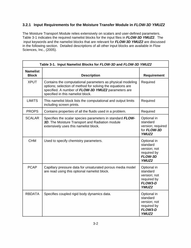
The Moisture Transport Module relies extensively on scalars and user-defined parameters. Table 3-1 indicates the required namelist blocks for the input files in FLOW-3D YMUZ2. The input keywords and the namelist blocks that are relevant for FLOW-3D YMUZ2 are discussedin the following section. Detailed descriptions of all other input blocks are available in FlowSciences, Inc., (2005).

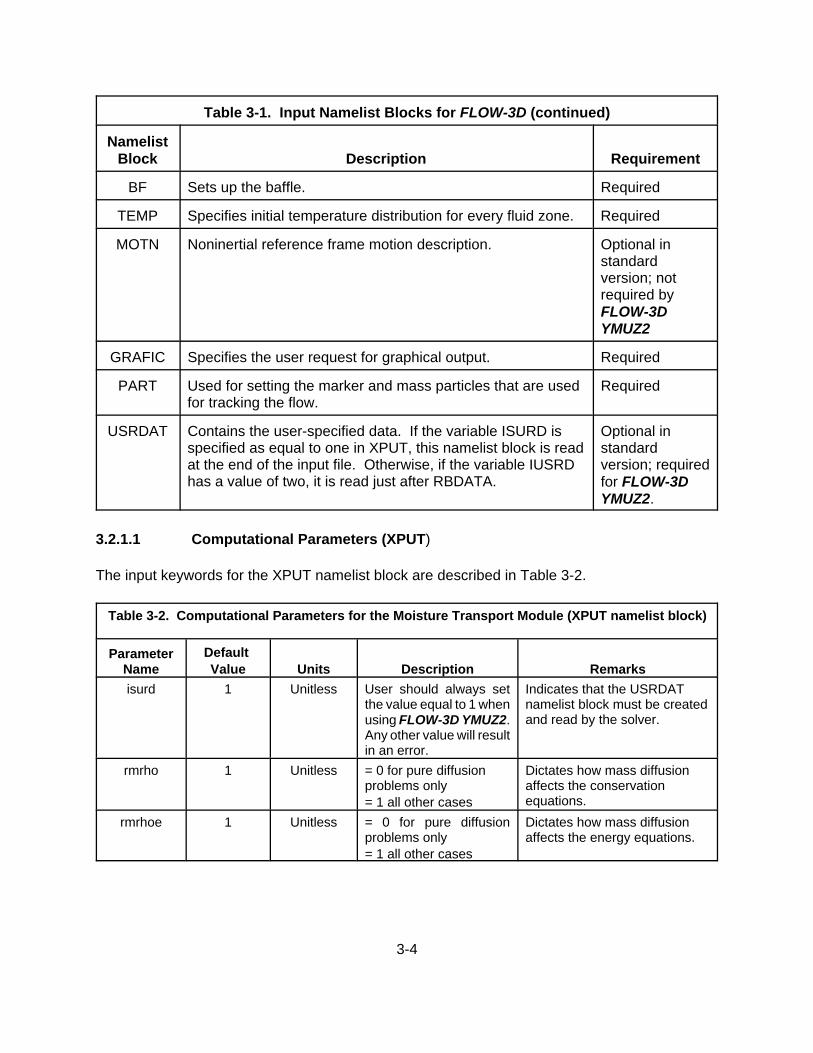
Table 3-1. Input Namelist Blocks for FLOW-3D and FLOW-3D YMUZ2

NamelistBlock Description Requirement

XPUT Contains the computational parameters as physical modelingoptions; selection of method for solving the equations arespecified. A number of FLOW-3D YMUZ2 parameters arespecified in this namelist block.

Required

LIMITS This namelist block lists the computational and output limitsincluding screen prints.

Required

PROPS Contains properties of all the fluids used in a problem. Required

SCALAR Specifies the scalar species parameters in standard FLOW-3D. The Moisture Transport and Radiation moduleextensively uses this namelist block.

Optional instandardversion; requiredfor FLOW-3DYMUZ2

CHM Used to specify chemistry parameters. Optional instandardversion; notrequired byFLOW-3DYMUZ2

PCAP Capillary pressure data for unsaturated porous media modelare read using this optional namelist block.

Optional instandardversion; notrequired byFLOW3-DYMUZ2

RBDATA Specifies coupled rigid body dynamics data. Optional instandardversion; notrequired byFLOW3-DYMUZ2

3-3

Table 3-1. Input Namelist Blocks for FLOW-3D and FLOW-3D YMUZ2 (continued)

Namelist Block Description Requirement

BCDATA Lists the boundary condition data. Needs to be specified foreach mesh block separately.

Required

MESH Specifies the mesh data. The computational domain couldcomprise multiple mesh blocks. The mesh data needs to bespecified for each unit.

Required

OBS Specifies the obstructions or geometries involved in theproblem.

Required

FL Specifies the fluid initial conditions for the problem. Therecould be multiple fluid zones in a problem, and each zoneneeds to be initialized separately.

Required

3-4

Table 3-1. Input Namelist Blocks for FLOW-3D (continued)

NamelistBlock Description Requirement

BF Sets up the baffle. Required

TEMP Specifies initial temperature distribution for every fluid zone. Required

MOTN Noninertial reference frame motion description. Optional instandardversion; notrequired byFLOW-3DYMUZ2

GRAFIC Specifies the user request for graphical output. Required

PART Used for setting the marker and mass particles that are usedfor tracking the flow.

Required

USRDAT Contains the user-specified data. If the variable ISURD isspecified as equal to one in XPUT, this namelist block is readat the end of the input file. Otherwise, if the variable IUSRDhas a value of two, it is read just after RBDATA.

Optional instandardversion; requiredfor FLOW-3DYMUZ2.

3.2.1.1 Computational Parameters (XPUT)

The input keywords for the XPUT namelist block are described in Table 3-2.

Table 3-2. Computational Parameters for the Moisture Transport Module (XPUT namelist block)

ParameterName

Default Value Units Description Remarks

isurd 1 Unitless User should always setthe value equal to 1 whenusing FLOW-3D YMUZ2.Any other value will resultin an error.

Indicates that the USRDATnamelist block must be createdand read by the solver.

rmrho 1 Unitless = 0 for pure diffusionproblems only= 1 all other cases

Dictates how mass diffusionaffects the conservationequations.

rmrhoe 1 Unitless = 0 for pure diffusionproblems only= 1 all other cases

Dictates how mass diffusionaffects the energy equations.

3-5

3.2.1.2 Fluid Properties (PROPS)

The input keywords for the PROPS namelist block describing the fluid properties are describedin Table 3-3.

Table 3-3. Fluid Properties for the Moisture Transport Module (PROPS namelist block)

ParameterName Default Value Units Description Remarksrhof 0.8463

[0.062]kg/m3

[lb/ft3]Nominal mixture densityfor energy equation

If the simulation showsthat the mixturetemperature is notconsistent with thespecified nominaldensity, a betterestimation may berequired. The defaultmay be changed basedon the requirement.

mu1 2.3543 ×10-5

[4.2 × 10-7]N-s/m2

[lbf-s/ft2]Nominal mixture dynamicviscosity

If the simulation showsthat the mixturetemperature is notconsistent with thespecified nominalviscosity, a betterestimation may berequired. The defaultmay be changed basedon the requirement.

thc1 0.03484[0.02]

W/m-K[BTU/hr-ft-°F]

Nominal mixture thermalconductivity

If the simulation showsthat the mixturetemperature is notconsistent with thespecified nominalthermal conductivity, abetter estimation may berequired. The defaultmay be changed basedon the requirement.

cv1 717 at 20 °C[0.172 at

68°F]

J/kg-K [BTU/lb-°F]

Constant volume- specificheat for dry air

This is a function of dryair temperature. Thedefault may be changedbased on therequirement.

3.2.1.3 User- Defined Scalars (SCALAR)

A SCALAR variable in FLOW-3D is a physical scalar quantity that is used to perform a numberof functions ranging from storing a variable to solving for a flow parameter associated with theprincipal flow. A number of scalars, known as active scalars, are used by the solver for models

3-6

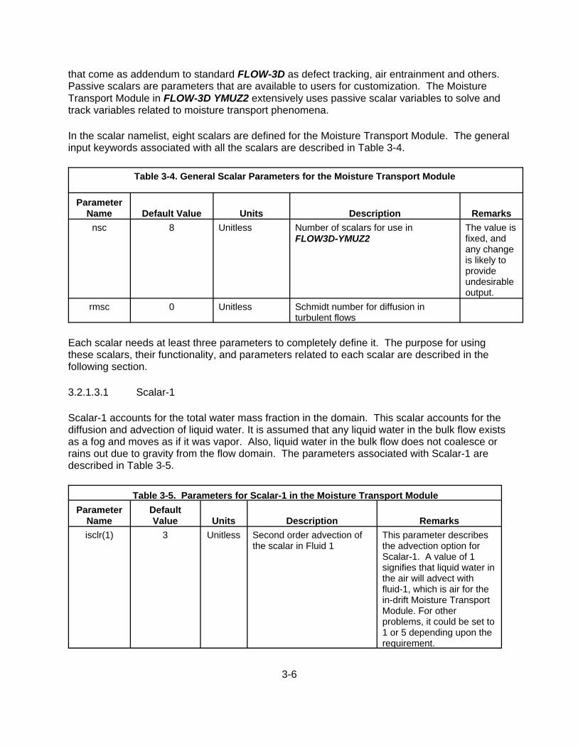
that come as addendum to standard FLOW-3D as defect tracking, air entrainment and others. Passive scalars are parameters that are available to users for customization. The MoistureTransport Module in FLOW-3D YMUZ2 extensively uses passive scalar variables to solve andtrack variables related to moisture transport phenomena.

In the scalar namelist, eight scalars are defined for the Moisture Transport Module. The generalinput keywords associated with all the scalars are described in Table 3-4.

Table 3-4. General Scalar Parameters for the Moisture Transport Module

ParameterName Default Value Units Description Remarks

nsc 8 Unitless Number of scalars for use inFLOW3D-YMUZ2

The value isfixed, andany changeis likely toprovideundesirableoutput.

rmsc 0 Unitless Schmidt number for diffusion inturbulent flows

Each scalar needs at least three parameters to completely define it. The purpose for usingthese scalars, their functionality, and parameters related to each scalar are described in thefollowing section.

3.2.1.3.1 Scalar-1

Scalar-1 accounts for the total water mass fraction in the domain. This scalar accounts for thediffusion and advection of liquid water. It is assumed that any liquid water in the bulk flow existsas a fog and moves as if it was vapor. Also, liquid water in the bulk flow does not coalesce orrains out due to gravity from the flow domain. The parameters associated with Scalar-1 aredescribed in Table 3-5.

Table 3-5. Parameters for Scalar-1 in the Moisture Transport ModuleParameter

NameDefaultValue Units Description Remarks

isclr(1) 3 Unitless Second order advection ofthe scalar in Fluid 1

This parameter describesthe advection option forScalar-1. A value of 1signifies that liquid water inthe air will advect withfluid-1, which is air for thein-drift Moisture TransportModule. For otherproblems, it could be set to1 or 5 depending upon therequirement.

3-7

Table 3-5. Parameters for Scalar-1 in the Moisture Transport Module (continued)Parameter


cmsc(1) 0.26 × 10!4

[0.17 × 10!4]kg/m-s[lb/ft-s]

Molecular diffusioncoefficient for Scalar-1

The default value is thediffusion coefficient ofliquid water in Fluid-1. Fluid-1 is air for studiesrelated to FLOW-3DYMUZ2.

scltit(1) Tot.Water Unitless Title of Scalar-1 The string input should bebetween the quotationmarks.

3.2.1.3.2 Scalar-2

Scalar-2 accounts for the mass flux at the wall. This scalar is used for extracting a field variablefor postprocessing. This variable holds the current water mass flux at each wall surface cell forrecording to the output data file so that the user can view/process the information. For example,total evaporation rate or condensation rate at a wall can be computed from data extracted fromFLOW-3D YMUZ2 and transferred to a spreadsheet. The scalar is only defined in the boundarysurfaces that have an interface with a solid wall. The input keywords associated with Scalar-2are discussed in Table 3-6.

Table 3-6. Parameters for Scalar-2 in the Moisture Transport Module Parameter


isclr(2) 0 Unitless No advection of the scalar This scalar is for extractingfield variable, liquid waterflux that is required for postprocessing. It is not used inthe solver. This parametervalue should not bechanged.

cmsc(2) 0 kg/m-s[lb/ft-s]


The molecular diffusionvalue is set to zero as thisscalar is only for accountinga field variable. Thisparameter value should notbe changed.

scltit(2) "Liq.Flux" Unitless Title of Scalar-2 The string input should bebetween the quotationmarks.

3.2.1.3.3 Scalar-3

Scalar-3 accounts for the relative humidity in the domain. This variable holds the current valueof relative humidity at all flow domains and boundary cells. This value is intended for

3-8

visualization of the humidity during a simulation and is extracted from the flow field. The inputkeywords associated with Scalar-3 are discussed in Table 3-7.


NameDefaultValue

Units Description Remarks

isclr(3) 0 Unitless No advection of the scalar This scalar is for extractingfield variable relativehumidity required for postprocessing; it is not used inthe solver. This parametervalue should not bechanged.

cmsc(3) 0[0]

kg/m-s[lb/ft-s]



scltit(3) "Rel.Hum" Unitless Title of Scalar-3 The string input should bebetween the quotationmarks.

3.2.1.3.4 Scalar-4

Scalar-4 accounts for the net water mass transferred at the wall, and like Scalar-2 and Scalar-3,it is also used to store variables for visualization. This variable accounts for the total mass ofwater that has changed phase at a wall. Initial transient values are also stored in this scalar. As a result, the initial values of Scalar-4 will tend to show nonphysical oscillations. To use thisvariable, it is suggested that a user perform a restart once the start-up transients are purged outand the flow stabilizes. The input keywords associated with Scalar-4 are discussed in Table 3-8.



isclr(4) 0 Unitless No advection of the scalar This scalar is for extractingfield variable total mass ofwater changing phase at thewall. It is not used in thesolver. This parametervalue should not bechanged.

3-9

Table 3-8. Parameters for Scalar-4 in the Moisture Transport Module (continued)Parameter


cmsc(4) 0 kg/m-s [lb/ft-s]

Molecular diffusion coefficientfor Scalar-4


scltit(4) '"Net.Liq" Unitless Title of Scalar-4 The string input should bebetween the quotationmarks.

3.2.1.3.5 Scalar-5

Scalar-5 saves the water vapor mass fraction in each cell of the computational domain and doesnot computationally interact with the solver. The initial value of water vapor mass fraction(i.e., Scalar-5) should be specified at the beginning of the simulation.

Table 3-9. Parameters for Scalar-5 in the Moisture Transport Module

ParameterName

DefaultValue Units Description Remarks

isclr(5) 0 Unitless No advection of the scalar This scalar accounts for thewater vapor mass fraction inthe domain. It is not used inthe solver. This parametervalue should not bechanged.

cmsc(5) 0[0]

kg/m-s [lb/ft-s]



scltit(5) "Vap.Wat" Unitless Title of Scalar-5 The string input should bebetween the quotationmarks.

3.2.1.3.6 Scalar-6

Scalar-6 is similar in nature to Scalar-5, but it stores liquid water mass fraction in thecomputational domain. It is also meant for accounting a field variable and post processing. Scalar-6 needs to be initialized, which will provide the solver with a value of liquid water massfraction at every grid point at the beginning of the solution.

3-10


ParameterName


isclr(6) 0 Unitless No advection of the scalar This scalar accounts for theliquid water mass fraction inthe domain. It is not used inthe solver. This parametervalue should not bechanged.

cmsc(6) 0 kg/m-s[lb/ft-s]



scltit(6) "Liq.Wat" Unitless Title of Scalar-7 The string input should bebetween the quotationmarks.

3.2.1.3.7 Scalar-7

Scalar-7 keeps track of the wall phase change calculation iterations and can be used fordebugging and troubleshooting. This scalar is defined only for wall surface cells. This variablecounts the number of iterations required to have a converged solution of vapor concentrationand wall temperature at each wall surface cell. This scalar is also useful for troubleshooting andcan be used to set the relaxation factor vaprlx.


ParameterName


isclr(7) 0 Unitless No advection of the scalar It keeps track of the numberof iterations required tohave a converged solutionof wall temperature andvapor concentration at thesurface. This parametervalue should not bechanged.

cmsc(7) 0 kg/m-s [lb/ft-s]



scltit(7) "Itr.Wall" Unitless Title of Scalar-7 The string input should bebetween the quotationmarks.

3-11

3.2.1.3.8 Scalar-8

Scalar-8 keeps track of the number of iterations required to adjust the bulk flow relativehumidity. It is similar in nature to Scalar-7 as it is also used for debugging and troubleshooting. The main function of Scalar-8 is to hold the current number of iterations required to have aconverged solution of vapor concentration and fluid temperature at each flow domain cell tosatisfy the energy– humidity constraint. Like Scalar-7, this variable is also useful fortroubleshooting and can be used to set the relaxation factor vaprlx.


ParameterName


isclr(8) 0 Unitless No advection of the scalar It keeps track of thenumber of iterationsrequired to have aconverged solution of fluidtemperature and vaporconcentration in the flowdomain. This parametervalue should not bechanged.

cmsc(8) 0[0]

kg/m-s[lb/ft-s]



scltit(8) "Itr.Mesh" Unitless Title of Scalar-8 The string input should bebetween the quotationmarks.

3.2.1.4 Flow Field Initialization (FL)

In the standard version of FLOW-3D, initialization of pressure is not mandatory. It is, however,a requirement for FLOW-3D YMUZ2 as a number of flow parameters are calculated based onthe initial pressure values. In addition, a number of user-defined scalars have to be initialized. It is possible to specify spatially varying initial values for these parameters as described in thestandard FLOW-3D Users Manual (Flow Sciences, Inc., 2005). Table 3-13 describes the inputkeywords related to the namelist block FL.

3-12

Table 3-13. Initialization Parameters for the Moisture Transport Module

ParameterName


presi 99379[2075.57]

Pa[lbf/ft2]

Initial uniform pressurein the flow domain

This parameter must be specified forFLOW-3D YMUZ2. The regularFLOW-3D solver can simulate flowwithout any initial uniform pressurespecification but initial uniformpressure must be specified inFLOW-3D YMUZ2 to calculatemixture parameters. The simulationwill provide an erroneous resultwithout an initial pressurespecification.

sclri(1) 0.022 Unitless Initial value of total watermass fraction in the flowdomain (Scalar-1)

Default value is for 100% relativehumidity at a pressure of 99.379 kPa[2075.57 lbf/ft2] and a temperature of299.7 K [79.79 °F].

sclri(5) 0.022 Unitless Initial value of watervapor mass fraction inthe flow domain (Scalar-5)

Default value is for 100% relativehumidity at a pressure of 99.379 kPa[2075.57 lbf/ft2] and a temperature of299.7 K [79.79 °F].

sclri(6) 0 Unitless Initial value of liquidwater mass fraction inthe flow domain (Scalar-6)

Default value is for 100% relativehumidity at a pressure of 99.379kPa [2075.57 lbf/ft2] and atemperature of 299.7 K [79.79 °F].

3.2.1.5 Temperature Field Initialization (TEMP)

The input parameters for the namelist block TEMP are described in Table 3-14.

Table 3-14. Temperature Field Initialization for the Moisture Transport Module

ParameterName


ntmp 1 Unitless Number of zones createdto specify initialtemperature. Each zonecould start with a distincttemperature.

This parameter depends upon thenumber of zones created tospecify initial temperatures. Thetypical value would be 1 for mostof the in-drift heat transfer simulations.

3-13

Table 3-14. Temperature Field Initialization for the Moisture Transport Module (continued)

ParameterName


tempi 299.7[79.79]

K[°F]

Initial uniformtemperature in thedomain

If multiple initial temperaturezones are created, each of themneeds to be initialized with thekeyword TREG.

3.2.1.6 User- Defined Parameters (USRDAT)

User-defined parameters used in FLOW-3D YMUZ2 are described in Table 3-15.

Table 3-15. User-Defined Parameters for the Moisture Transport Module

ParameterName

Default ValueUnits Description Remarks

istwtf_stg "tw" Unitless "tw" for wall source"tf" for fluid source

This string input parameterdefines the source of energyrequired for the phasechange.

imoist_stg(n) -n Unitless This parameterdefines obstacles thatcan condense andevaporate withoutlimit. These areessentially saturatedporous surfaces. Thisis an array input andshould be defined forevery condensing orevaporating surfaces.

This parameter needs to bespecified for any surface thatparticipates in thecondensation-evaporationprocess.

ilqonly_stg(n) -n Unitless This parameterdefines obstacles thatcan condense withoutlimit. These surfacescan also reevaporatethe condensed wateras long as it isavailable.

This parameter needs to bespecified for any surface thatparticipates in thecondensation-evaporationprocess.

isvap_stg 1 Unitless Defines scalar indexfor waterconcentration.

The default value should notbe changed.

isliq_stg 2 Unitless Defines scalar indexfor liquid flux.


isrh_stg 3 Unitless Defines scalar indexfor relative humidity.


istlq_stg 4 Unitless Defines scalar indexfor total liquidaccumulation.


3-14

Table 3-15. User Defined Parameters for the Moisture Transport Module (continued)Parameter

Name Default Value Units Description Remarksisywv_stg 5 Unitless Defines scalar index

for liquid water (mist).The default value should notbe changed.

hvvap_stg 2304900[990.96]

J/kg[BTU/lb]

Energy of vaporizationof water.

Parameter value depends onthe specific range oftemperature in the simulation.

cvvap_stg 1370 [0.3272] J/kg-K [BTU/lb-°F]

Constant volumespecific heat for watervapor.


cvliq_stg 4186 [1]

J/kg-K [BTU/lb-°F]

Constant volumespecific heat for liquidwater.


rvap_stg 416[0.01]

J/kg-K [BTU/lb-°F]

Gas constant for watervapor.


rgas_stg 289 [6.9×10-2] J/kg-K [BTU/lb-°F]

Gas constant for air. Parameter value depends onthe specific range oftemperature in the simulation.

vaprlx_stg 0.8 Unitless Relaxation factor forphase changeiterations.

Parameter value depends onstability and other numericalconsiderations.

rhlim_stg "y" Unitless y (Limit relativehumidity to 100%)n (Do not limit relativehumidity)

"y" option sets a limit ofrelative humidity to 100%,and any excess water vaporwill condense and advect asfog beyond saturation limit."n" option will allowsupersaturation of air.

3.2.2 Input Requirements for Radiation Module in FLOW-3D YMUZ2

The Radiation Module of FLOW-3D YMUZ2 requires a number of input keywords that aredescribed in this section. Some of the keywords are common to the Moisture Transport Module. The Radiation module could, however, be used independent of the Moisture Transport Module.

3.2.2.1 Computational Parameters (XPUT)The radiation module input parameters for the namelist block XPUT are provided in Table 3-16.

Table 3-16. Computational Parameters for the Radiation ModuleParameter


isurd 1 Unitless User should always set thevalue equal to 1 when usingFLOW-3D YMUZ2. Any othervalue will result in an error.

Indicates that the USRDATnamelist block must becreated and read by thesolver.

3-15

3.2.2.2 User- Defined Parameters (USRDAT)

Almost all the user-defined parameters in the Radiation Module deal with the geometry andorientation of the solid objects and surfaces participating in the radiation heat transfer process. A generalized schematic is shown in Figure 3-1 to explain the input keywords related to theuser- defined parameters in the Radiation Module. The schematic shows a number of solidobjects placed side by side. These objects can have any arbitrary orientation in space. Figure3-1 has line orientation relevant to Yucca Mountain disposal plans currently considered by DOE. Each object is identified with an index "m" and contains a number of radiating surfaces identifiedwith an index "n". It is not necessary for every surface of an object to participate in radiation. Only those surfaces that take part in radiation are identified with the index "n". For example,only surface n = 4 participates in the radiation heat transfer on the object m = 2. None of thesurfaces in object m = 4 take part in the radiation heat transfer process. It is also possible tosubdivide a continuous surface with some subdivisions participating in radiation while othersstay inert. Table 3-17 provides the input parameters for the namelist block USRDAT.

3.3 Output from FLOW-3D YMUZ2

The FLOW-3D GUI is used to graphically display the computational domain, geometricalparameters, and flow field variables. Values such as temperature, pressure, water vaporconcentration, and relative humidity can be presented in contour plots. The use of the standardflow visualization GUI tool has certain limitations with respect to the Moisture Transport andRadiation Modules. The standard visualization tool cannot compute the heat transfer due tophase change or radiation. The user needs to perform some additional calculations to extractand visualize these parameters. In the case of the Radiation Module, a special file is created torecord the radiation-specific input parameters and to record the values of the radiation heattransfer rates from each radiation surface. These heat transfer rates can be used to computequantities such as total heat transfer rate.

Figure 3-1. Schematic for an Arrangement of Solid Bodies With Radiating Surfaces

3-16

Table 3-17. User-Defined Parameters for the Radiation Module

ParameterName


srsrf_stg 1 Unitless Number of radiatingsurfaces

This parameter is only usedwhen the code calculatesthe configuration factors.

eps_stg(n) 0.9 Unitless Emissivity of surfacenumber "n"

If the emissivity of surface n= 1 is 0.9 and that ofsurface n = 2 is 0.9, theneps_stg (1) = 0.9 andeps_stg (2) = 0.95.

rad_stg(1,n) Unitless The obstacle number thathas surface “n”

As shown in Figure 3-1,object m = 3 containssurface n = 5; hence.rad_stg (1,5) = 3.

rad_stg(2,n) m Lower x-limit of cells onradiation surface "n"

For surface 5 rad_stg, (2,5)will be the minimum xcoordinate value of thesurface.

rad_stg(3,n) m Upper x-limit of cells onradiation surface "n"

For surface 5 rad_stg, (2,5)will be the maximum xcoordinate value of thesurface.

rad_stg(4,n) m Lower y-limit of cells onradiation surface "n"

For surface 5 rad_stg, (2,5)will be the minimum ycoordinate value of thesurface.

rad_stg(5,n) m Upper y-limit of cells onradiation surface "n"

For surface 5 rad_stg, (2,5)will be the maximum ycoordinate value of thesurface.

rad_stg(6,n) m Lower z-limit of cells onradiation surface "n"

For surface 5 rad_stg, (2,5)will be the minimum zcoordinate value of thesurface.

rad_stg(7,n) m Upper z-limit of cells onradiation surface "n"

For surface 5 rad_stg (2,5)will be the maximum zcoordinate value of thesurface.

iusrcf_stg 0 Unitless = 0 for configuration factors are computed by the code= 1 for configuration factors are specified by the user

Provides user a choice ofeither reading theconfiguration factors thatwere calculated externallyand provided as input orcalculate it within FLOW-3D YMUZ2.

3-17

Table 3-17. User Defined Parameters for the Radiation Module (continued)

ParameterName


cf_stg(i,j) Unitless User-specified value ofradiation configurationfactor, Fn-m

This option is onlyfunctional if iusrcf_stg = 0These configuration factorscould be calculatedexternally and supplied asan input. If the viewconfiguration factorbetween surfaces 3 and 4is 0.2 then cf_stg (3,4) =0.2.

3.3.1 Output from the Moisture Transport Module

All of the scalar variables defined in the "$Scalar" namelist block can be viewed as contour plotsin the FLOW-3D graphics package. These values can also be extracted into text files forpostprocessing. To compute the energy transfer via mass transfer, the user must extract thefollowing values for the surfaces in question:

• Fluid temperature• Wall temperature• Heat transfer coefficient• Liquid flux (variable specific to Moisture Transport Module)

Conductive and convective heat flux at each cell are computed by the FLOW-3D YMUZ2postprocessor. The energy transfer via phase change has to be computed externally such asby Microsoft® Excel® ( Microsoft Corporation, 2002b) using the values listed previously obtainedfrom the FLOW-3D YMUZ2 solutions from the total energy values at each cell.

3.3.2 Output from the Radiation Module

Subroutines rad_init and rad_calc were modified to record the pertinent output information fromthe Radiation Module. These modifications are given in the file check_rad.* where * stands forthe problem being executed as is the case with the other problem-specific FLOW-3D files. Theconfiguration factor matrix terms and the time history of the radiation heat transfer rates of thesurfaces that are activated for radiation information are recorded in this file.

4-1

4 SAMPLE PROBLEM

This section provides an example for the use of the Moisture Transport and Radiation Modules. This sample problem is identical to one of the test cases described in Green (2006). It isintended for demonstration purposes, not for testing all code capabilities.

4.1 Problem Description

The objective of this test is to estimate the heat transfer rate due to conduction, convection, andradiation along with the mass transport rate due to phase change in a heated enclosure. Thevertical walls of the enclosure participate in the radiative heat transfer and provide the source ofwater. The horizontal surfaces are treated as adiabatic hydrophobic walls.

A two-dimensional enclosure measuring 0.1 × 0.1 m [0.32 × 0.32 ft] is depicted in Figure 4-1. The left vertical wall is 0.025 m [8.2 × 10!2 ft] thick and has an internal heat generation rate suchthat the heat flux at the inner surface is 200 W/m2 [63.4 BTU/hr-ft2]. The outer surface of thiswall is adiabatic. The right vertical wall is 0.025 m [8.2 ×10!2 ft] thick, and its outer surface isheld constant at 300 K [80.3 °F]. The emissivity of both the left and right walls is 0.9. Thevertical walls provide for the evaporation and condensation of water as needed under the localtemperature and concentration conditions in the flow. The upper and lower walls are adiabaticand do not exchange heat with the vertical walls. These walls are assumed to be transparent toradiation and, therefore, do not interact with the other walls via this mode. These walls arefurthermore assumed to not be a source or a sink for water. The only interaction of these wallsin the problem is to bound the flow and provide for viscous drag. The acceleration due togravity is assumed to be only 0.001 × g (g is the gravitational constant) so that the flow field forthese geometric and thermal conditions will be laminar.

The objective here is to compare the effects of the radiation and moisture transport processesto accurately model a turbulent flow scenario. The fluid and wall properties used in thissimulation are listed in Table 4-1.

The density value listed above is used as the nominal density in the conservation of energyequation. The incompressible ideal gas model is used for this test case for the temperature-and concentration-dependent density that is used for the momentum equation. The MoistureTransport Module parameters used in this study are described in Table 4-2.

4.2 Test Cases

The following four cases will be investigated:

(1) Convection only(2) Convection with radiation(3) Convection with moisture transport(4) Convection, radiation, and moisture transport.

4-2

Figure 4-1. Schematic for Convection, Radiation, and Mass Transfer in aTwo-Dimensional Enclosure

[1 m = 3.28 ft; 1 W/m3 = 9.66 × 10-2 BTU/hr/ft3; °F = 1.8 × T K - 459.67]

Table 4-1. Fluid and Wall Properties for the Combined Heat and Moisture TransportProblem in an Enclosure

Property ValueViscosity (:) 2 ×10-5 Pa-sec [4.16 ×10-7 lbf-s/ft2]

Fluid thermal conductivity (kair) 0.026 W/m-K [0.015 BTU/hr-ft-°F]Air/Vapor diffusivity (D) 2.6 ×10-5 m2/sec [26.5 ×10-5 ft2/sec]

Nominal Density (D) 1.169 kg/m3 [0.073 lb/ft3]Wall thermal conductivity (kw) 1 W/m-K [0.58 BTU/hr-ft-°F]

4-3

rmrhoe=1., remark='Density diffusion term coefficient', rmrho=1., remark='Energy diffusion term coefficient', remark=' RMRHO, RMRHOE REQUIRED FOR VAPOR TRANPORT MODEL ', iusrd=1,

Table 4-2. Moisture Transport Module Parameters Used in the Combined Heat andMoisture Transport Problem in an Enclosure

Property ValueHeat of vaporization of water (ufg) 2,304,900 J/kg [990.94 BTU/lb]

Water vapor-specific heat (Cvv) 1370 J/kg-K [0.33 BTU/lb-°F]Liquid water-specific heat (Cvl ) 2.6 × 0-5 m2/sec [26.5 ×10-5 ft2/sec] Water vapor gas constant (Rv) 416 J/kg-K [1 ×10-2 BTU/lb-°F]

Air gas constant (Ra) 289 J/kg-K [6.9 ×10-2 BTU/lb-°F]

The input file for Case 4, which simulates the enclosure for convection, radiation, and moisturetransport, is provided here. Input parameters that are specific to the Moisture Transport andRadiation Modules are highlighted and enclosed in boxes. The input file for the other three testcases is provided in Appendix C. Users can use these input files to test the installation ofFLOW-3D YMUZ2.

4.3 Input File for Convection With Moisture Transport and Radiation

Heat transfer in 2-D Sq. Box w/ natural convection, radiation, moisture Ra ~ 6000 for natural convection only Box is 0.1 m x 0.1 m long, Adiabatic at top and bottom, 20 W generated in left wall, 300 K at outer face of right wall. Both walls have k=1 w/(m*K), rcobs=1000*joule/(m^3*K) Moisture at left and right walls if modeled Radiation at left and right walls if modeled

$xput remark='units are SI', itb=0, remark='Sharp interface not required', ifvis=0, remark='Laminar', ifenrg=2, remark='Solve energy eq., first order', ifrho=1, remark='Temp. dependent density', gz=-9.8e-03, remark='Gravity', ipdis=1, remark='Hydrostatic prfessure distribution in z-direction', ihtc=2, remark='Evaluate heat transfer with solid conduction', iwsh=1, remark='Wall shear active', delt=1.e-4, remark='', twfin=4000., remark='',

$end

$limits

$end

$props

4-4

thc1=0.026, remark='Bulk nominal thermal conductivity for energy equation', thexf1=0.003226, remark='Approximate thermal expansion coefficient', tstar = 300., remark='Reference temperature for thermal expansion coefficient', remark='THEXF1, TSTAR not needed for vapor tranport model', remark='but are used in some parts of code to set up simulation',

nsc=8, isclr(1)=3, cmsc(1)=0.26e-04, scltit(1)='Tot.Water', rmsc=0., isclr(2)=0, cmsc(2)=0., scltit(2)='Liq.Flux', isclr(3)=0, cmsc(3)=0., scltit(3)='Rel.Hum', isclr(4)=0, cmsc(4)=0., scltit(4)='Net.Liq', isclr(5)=0, cmsc(5)=0., scltit(5)='Vap.Wat', isclr(6)=0, cmsc(6)=0., scltit(6)='Liq.Wat', isclr(7)=0, cmsc(7)=0., scltit(7)='Itr.Wall', isclr(8)=0, cmsc(8)=0., scltit(8)='Itr.Mesh',

units='si',

rhof=1.1687, remark='Bulk nominal density at 310 K for energy equation', mu1=2.e-05, remark='Bulk nominal dynamic viscosity density for momentum equation', cv1=717., remark='Const. Vol. Specific heat of dry air',

$end

$scalar remark='Water vapor scalars not used for this problem but need to be defined to use the ', remark=' radiation and water transport modules together', remark='Scalar 1 is the diffusing/advecting water', remark='Scalar 2 (non-diffusing) is for storing the surface phase change flux values', remark='Scalar 3 (non-diffusing) is for storing the relative humidity values', remark='Scalar 4 (non-diffusing) is for storing the net surface liquid accumulation', remark='Scalar 5 (non-diffusing) is for storing the vapor water concentration', remark='Scalar 6 (non-diffusing) is for storing the liquid water (mist) concentration', remark='Scalar 7 (non-diffusing) is for storing the calculation iterations for the', remark=' wall mass flux', remark='Scalar 8 (non-diffusing) is for storing the calculation iterations for the', remark=' mist phase change in the fluid interior', remark='Scalars 7 and 8 are helpful in tuning the value of vaprlx if necessary',

$end

$bcdata wl=1, remark='Symmetry at left to make all the heat go into the inner face', wr=2, remark='Constant temperature wall at right', tbc(2)=300., wf=1, wbk=1, remark=' Symmetry at front and back', wb=2, remark=' Insulated wall', wt=2, remark=' Insulated wall', $end

$mesh px(1) =-0.025, py(1) =0.0, pz(1) = 0.0, px(2) = 0.0, py(2) =1., pz(2) = 0.1, px(3) = 0.1, px(4) = 0.125, nxcell(1)=5, nxcell(2)=20,

4-5

remark=' No vapor in fluid', sclri(1)=0.0, sclri(5)=0.0, sclri(6)=0.0, presi=101325.,

ntmp=1, tempi=300., presi=101325.,

nxcell(3)=5, nxcelt= 30, nycelt=1, nzcelt=30, $end

$obs avrck=-3.1, nobs = 2, tobs(1)=0., tobs(2)=1000., remark='Obstacle 1. Left channel wall. Total heat output 50W', xl(1)=-0.025, xh(1)=0., kobs(1)= 1., rcobs(1)=10000., twobs(1,1)=300., pobs(1,1)=20., pobs(2,1)=20., remark='Obstacle 2. Right channel wall. Conduction to constant temp', xl(2)=0.1, xh(2)=0.125, kobs(2)= 1., rcobs(2)=10000., twobs(1,2)=300., $end

$fl

$end

$bf

$end

$temp

$end

$motn

$end

4-6

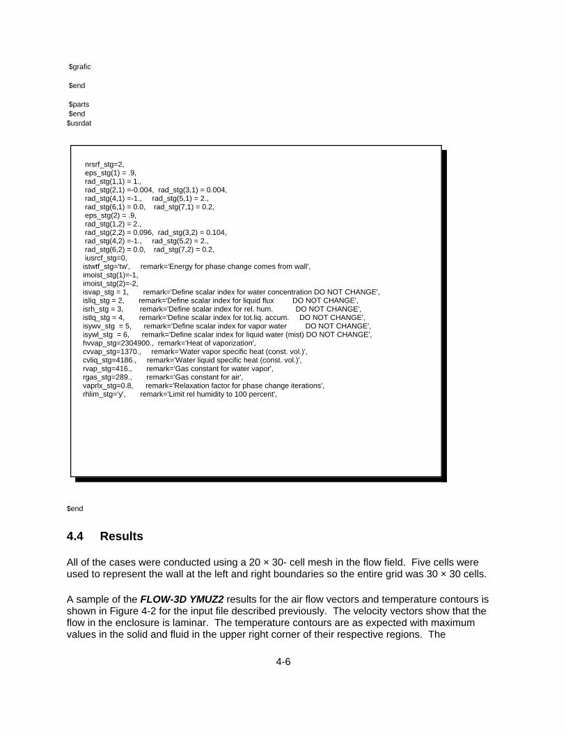
nrsrf_stg=2, eps_stg(1) = .9, rad_stg(1,1) = 1., rad_stg(2,1) =-0.004, rad_stg(3,1) = 0.004, rad_stg(4,1) =-1., rad_stg(5,1) = 2., rad_stg(6,1) = 0.0, rad_stg(7,1) = 0.2, eps_stg(2) = .9, rad_stg(1,2) = 2., rad_stg(2,2) = 0.096, rad_stg(3,2) = 0.104, rad_stg(4,2) =-1., rad_stg(5,2) = 2., rad_stg(6,2) = 0.0, rad_stg(7,2) = 0.2, iusrcf_stg=0, istwtf_stg='tw', remark='Energy for phase change comes from wall', imoist_stg(1)=-1, imoist_stg(2)=-2, isvap_stg = 1, remark='Define scalar index for water concentration DO NOT CHANGE', isliq_stg = 2, remark='Define scalar index for liquid flux DO NOT CHANGE', isrh_stg = 3, remark='Define scalar index for rel. hum. DO NOT CHANGE', istlq_stg = 4, remark='Define scalar index for tot.liq. accum. DO NOT CHANGE', isywv_stg = 5, remark='Define scalar index for vapor water DO NOT CHANGE', isywl_stg = 6, remark='Define scalar index for liquid water (mist) DO NOT CHANGE', hvvap_stg=2304900., remark='Heat of vaporization', cvvap_stg=1370., remark='Water vapor specific heat (const. vol.)', cvliq_stg=4186., remark='Water liquid specific heat (const. vol.)', rvap_stg=416., remark='Gas constant for water vapor', rgas_stg=289., remark='Gas constant for air', vaprlx_stg=0.8, remark='Relaxation factor for phase change iterations', rhlim_stg='y', remark='Limit rel humidity to 100 percent',

$grafic

$end

$parts $end$usrdat

$end

4.4 Results

All of the cases were conducted using a 20 × 30- cell mesh in the flow field. Five cells wereused to represent the wall at the left and right boundaries so the entire grid was 30 × 30 cells.

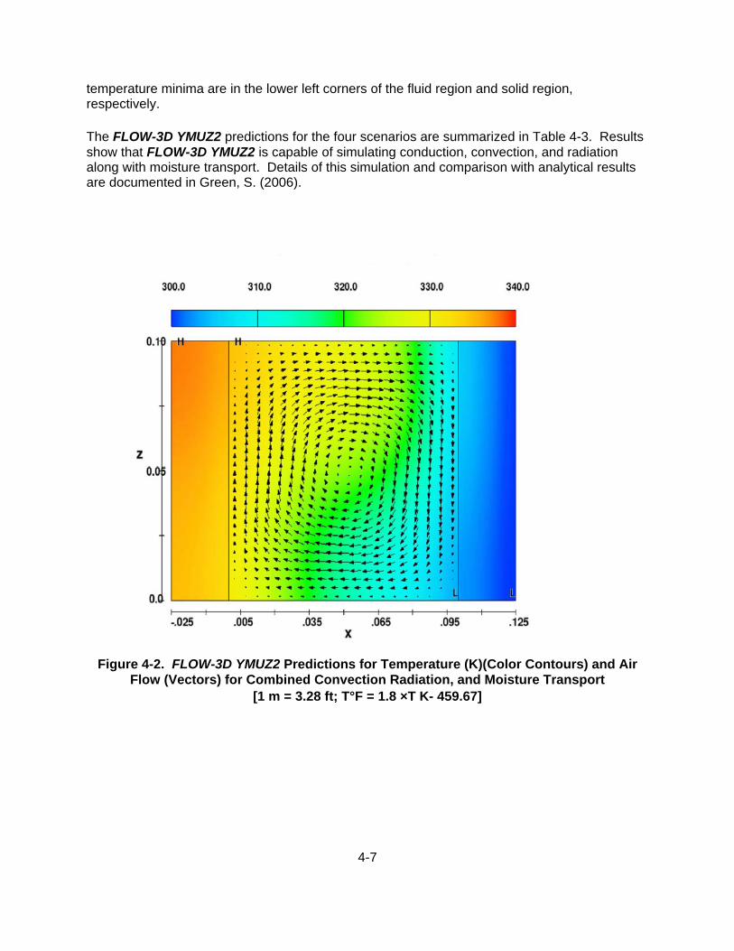
A sample of the FLOW-3D YMUZ2 results for the air flow vectors and temperature contours isshown in Figure 4-2 for the input file described previously. The velocity vectors show that theflow in the enclosure is laminar. The temperature contours are as expected with maximumvalues in the solid and fluid in the upper right corner of their respective regions. The

4-7

temperature minima are in the lower left corners of the fluid region and solid region,respectively.

The FLOW-3D YMUZ2 predictions for the four scenarios are summarized in Table 4-3. Resultsshow that FLOW-3D YMUZ2 is capable of simulating conduction, convection, and radiationalong with moisture transport. Details of this simulation and comparison with analytical resultsare documented in Green, S. (2006).

Figure 4-2. FLOW-3D YMUZ2 Predictions for Temperature (K)(Color Contours) and AirFlow (Vectors) for Combined Convection Radiation, and Moisture Transport

[1 m = 3.28 ft; T°F = 1.8 ×T K- 459.67]

4-8

Table 4-3. FLOW-3D YMUZ2 Results for 2-D Enclosure Heat and MassTransfer Problem

Scenario

Th, HotSurface

TemperatureAverage(K)*

Tc, ColdSurface

TemperatureAverage(K)*

Heat Transfer Rate

MassTransfer(kg/m-s)‡

Convection (W/m)† Radiation

(W/m)†

PhaseChange(W/m)†

Total(W/m)†

ConvectionOnly

646.2 304.5 20 n/a n/a 20 n/a

Convection +Radiation

362.7 304.5 2.3 17.7 n/a 20 n/a

Convection +MoistureTransport

340.9 304.5 1.8 n/a 18.2 20 7.9 × 10!6

Convection +Radiation +

MoistureTransport

333.8 304.5 1.3 7.9 11 20.2 4.8 × 10!6

*° F = 1.8 × T K-459.67†W/m = 1.04 BTU/hr-ft‡kg/m-s = 0.67 lb/ft-s

5-1

5 REFERENCES

Bechtel SAIC Company, LLC. “Multiscale Thermohydrologic Model.” ANL–EBS–MD– 000049.Rev.03. Las Vegas, Nevada: Bechtel SAIC Company, LLC. 2005.

Flow Sciences, Inc., “FLOW-3D User Manual.” Version 9.0. Santa Fe, New Mexico: FlowSciences, Inc., 2005.

Green, S. “Software Validation Test Results for FLOW-3D Version 9.0.” San Antonio, Texas: CNWRA. 2006.

Manepally, C., A. Sun, R. Fedors, and D. Farrell. “Drift-Scale Thermohydrological ProcessModeling—In-Drift Heat Transfer and Drift Degradation.” CNWRA 2004-05. San Antonio, Texas:CNWRA. 2004.

Microsoft Corporation. “Microsoft® Windows XP® 2002.Service Pack.” Redmond, Washington:Microsoft Corporation. 2002a.

Microsoft Corporation. “Microsoft® Excel® 2002.5P3.” Redmond, Washington: MicrosoftCorporation. 2002b.

APPENDIX A

A–1

THEORETICAL BASIS OF THE MOISTURE TRANSPORT AND RADIATIONMODULES

Appendix A presents the theoretical basis for the Moisture Transport and Radiation Module.This discussion includes the evaluation techniques for different flow variables in the FLOW-3DYMUZ2 solver, proof of concept calculations, and solution schemes.

A1 MOISTURE TRANSPORT MODULE

The theory used to represent processes associated with the moisture transport in FLOW-3DYMUZ2 is described in this section. The equations for estimating the fluid density are discussedin Section A1.1 followed by the methodology to estimate the total energy in Section A1.2. Section A1.3 describes the method to calculate temperature. The governing equations for themass transfer and heat transfer rates associated with the Moisture Transport Modules arepresented in Section A1.4.

A1.1 Density Evaluation

The bulk density of the air/vapor mixture is obtained from engineering psychometrics (e.g.,ASHRAE, 1977) with the modification that allows for some water to be condensed as a mist in themixture. The species diffusion equation solved in FLOW-3D YMUZ2 is in terms of the mass fractionof the air and water. Hence, the density property in FLOW-3D YMUZ2 must be defined in termsof the mass fractions of these constituents.

The bulk density is defined as

ρ = =+ +m

Vm m m

Vtot a wv wl

(A–1)

where

mtot = total mass of all species in sample volume [kg]ma = mass of air [kg]mwv = mass of water vapor [kg]mwl = mass of water mist [kg]V = sample volume [m3]

A–2

mP VR T

P VR T

PVR T

xaa g

a

a

a aag= ≈ =

mP VR T

P VR T

PVR T

xwvwv g

v

wv

v vwvg= ≈ =

The mass of air is computed from the ideal gas equation of state along with the approximationthat the gas-only volume nearly equals the total volume

(A–2)

where

Pa = partial pressure of air [Pa]P = total static pressure [Pa]Ra = ideal gas constant for air = 287 J/kg-K [6.85 × 10-2 BTU/lb-°F]xag = mole fraction of air in the gas/vapor portion of the volumeVg = volume of gas only in control volume [m3]T = temperature [K]

Likewise, the mass of water vapor is

(A–3)

where

Pwv = partial pressure of water vapor [C"]Rv = ideal gas constant for water vapor {462 J/(kg-K) [0.11 BTU/lb/°F]}xwvg = mole fraction of air in the gas/vapor portion of the volume

The mass fractions of the vapor water and liquid water are computed as part of the humiditycalculations and are known inputs to the density evaluation algorithm. The mass fractions ofwater vapor and air in the gas phase can now be defined using Eqs. (A–4a) and (A–4b),respectively

( )cc

c cc

c 1 cwvgwv

wv a

wv

wv w

=+

=+ −

(A–4a)

and

c 1 cag wvg= − (A–4b)

where

ca = mass fraction of aircw = mass fraction of watercwv = mass fraction of water vaporcag = mass fraction of air vapor in gascwvg = mass fraction of water vapor in gas

A–3

xc

MM

1 c 1MM

wvg

wvga

w

wvga

w

=− −

⎛⎝⎜

⎞⎠⎟

ρ ρ= + +⎡

⎣⎢

⎤

⎦⎥ = +

⎛⎝⎜

⎞⎠⎟ +

1V

PVR T

xPVR T

x c mPT

xR

xR

ca

agw

wvg wl totag

a

wvg

wwl

( )ρ =−

+⎛⎝⎜

⎞⎠⎟

PT 1 c

xR

xR

wl

ag

a

wvg

w

e c C T c C T c ha va wv vv wl vap= + −

The respective mole fractions for water vapor and air in only the gas space can now be definedusing Eqs. (A–5a) and (A–5b), respectively

(A–5a)

and

x 1 xag wvg= − (A–5b)

where

Ma = molecular weight of airMw = molecular weight of water

Substituting Eq. (A–2) – Eq. (A–5b) in Eq. (A–1) gives

(A–6)

which can be reduced to

(A–7)

Eqs. (A–7) and (A–6) serve as the basis for evaluating the bulk density in the Moisture TransportModule. The inputs to this function are the local pressure, temperature, water vapor mass fraction,and liquid water (as mist) mass fraction.

A1.2 Air/Water Vapor Energy

The energy of an air/water mixture is evaluated following the basic procedures of standard FLOW-3D Version 9.0 (Flow Sciences, Inc., 2005). In this case, the mass-specific energy (e.g., J/kg) is a function of the local temperature and constituent concentrations

(A–8)

where

cwl = mass fraction of liquid water (as mist)T = temperature (K)

A–4

( )ρ ρI enom=

( )T

Ic h

c C c Cnom

wl vap

a va wv vv=

+

+

ρρ

( )ρ∂∂

∂∂

∂∂

∂∂

ρ ct

cx

cy

cz

D c mw w w wva w source

/ / /+ + +⎛⎝⎜

⎞⎠⎟= ∇ ⋅ + &

&msource/ / /

Cva = specific heat of air at constant volume (J/kg-K)Cvv = specific heat of water vapor at constant volume (J/kg-K)hvap = energy of vaporization of water (J/kg)

A1.3 Temperature Evaluation Method

The conservation of energy equation used in FLOW-3D is based on the volume-specific energydefined as the product of the nominal fluid density and the mass-specific energy

(A–9)where

(DI) — volume-specific energyDnom — constant nominal density provided by the user in the problem setupe — mass-specific energy for the air/water mixture

The (DI) product is the conserved quantity, and the temperature is calculated from thisparameter for use in various property functions and output files. Consequently, the temperatureevaluation function in FLOW-3D must be modified when using the Moisture Transport Model inwhich the mass-specific energy is different from the standard FLOW-3D installation. The mass-specific energy equation, Eq. (A–8), can be rearranged as

(A–10)

A1.4 Air/Water Vapor Energy

The Moisture Transport Module will be based on the well-established approach of theconservation of mass of multiple chemical species in nonreacting mixtures (Bird, et al., 1960). Aconservation equation for the transport of water vapor can be written as

(A–11)

where

D — bulk density of the air/water mixture (kg/m3)

u,v,w — vector components of bulk fluid flow (m/s)

x,y,z — coordinate directions (m)

Dva — diffusion coefficient for air/vapor (m2/s)

— volume specific rate of vapor generation (kg/m3-s)

A–5

The FLOW-3D software solves this equation in conjunction with the equations for theconservation of mass and momentum of the air/vapor mixture. The Moisture Transport Moduledoes not directly specify the source term in Eq. (A–11) for the mass transfer rate at walls. Rather, the module essentially provides the boundary conditions for Eq. (A–11) at wall surfaces. The methodology is described next.

A1.4.1 Phase Change at Walls

The scenario for mass transfer at a wall is shown in Figure A–1.

Figure A–1. Phase Change Process at Walls

The conservation of energy is applied to the solid wall and the liquid film on the wall over asingle timestep in the calculation. Evaporation or condensation will take place as necessary tosatisfy the energy change of the solid material. Any heat transfer to or from the air/vapormixture takes place via conduction/convection at the wall; the air/vapor mixture next to the walldoes not exchange energy directly with the water that is undergoing the phase change.

A–6

me e

tm hs

s,2 s,1w vap

−=

Δ&

ρs s ss,2 s,1

w vapC VT T

tm h

−=

Δ&

( )&m D Adcdx

D c cAVw,d va w va w,sat w

w2

f= ≈ −ρ ρ

Based on these assumptions, the conservation of energy can be expressed as

(A–12)

where

ms — mass of solid wall inside the control volume (kg)— mass flow rate of water evaporating/condensing (kg/s)&mw

es,1 — mass-specific energy of solid at the beginning of the timestep (J/kg)es,2 — mass-specific energy of solid at the end of the timestep (J/kg)Ds — solid material density (kg/m3)Cs — solid material specific heat (J/(kg-k)Vs — solid material volume (m3)hvap — heat of vaporization (J/kg))t — timestep (s)Ts,1 — wall temperature at beginning of timestepTs,2 — wall temperature at end of timestep

There are two unknowns in Eq. (A–12); namely, Ts,2 and . The mass flow rate of water&mwcould be obtained in two different ways: (1) It can be estimated from the diffusion flux of water vapor from the wall into the control

volume adjacent to the wall. The diffusion flow of vapor is estimated from anapproximation to the Fickian diffusion law (Bird, et al., 1960)

(A–13)

where

— mass flow via diffusion (kg/s)&mw,d

cw,sat — mass fraction of water vapor at saturation cw — current mass fraction of water vaporAw — wall surface area inside the cell (m2)Vf — volume of fluid in the cell (m3)Dva — diffusion coefficient for air/vapor (m2/s)D — bulk density of mixture (kg/m3 )

(2) could also be quantified as the mass flow of water that will create a saturated&mw

air/vapor mixture in the control volume at the corresponding fluid temperature. The masstransfer rate is estimated from the change in water content required to bring the vaporconcentration to the saturation value. Based on the law of conservation of mass, the flow

A–7

( )&m c cV

tw,s sat w,sat wf= −ρ ρ

Δ

( ) ( ) ( )ρ ρ ρI I c C T c C T c h2 1 nom a,1 va 1 wv,1 vv 1 wl,1 vap= = + −

rate required to saturate the air/vapor mixture adjacent to the wall in a singlecomputational timestep is estimated as

(A–14)

where

— mass flow required to saturate grid cell (kg/s)& ,mw s

D sat — bulk density at saturation condition (kg/m3 )cw,sat — mass fraction of water at saturation condition (kg/m3 )D — current bulk density of mixture (kg/m3 )cw — current mass concentration of water vapor (kg/m3 )Vf — fluid volume in the grid cell (m3))t — timestep(s)

The phase change rates from Eq. (A–13) and (A–14) are compared. The minimum of the twovalues is used in Eq. (A–12) to solve for Ts,2 and &mw

This process allows for the source terms of water mass into and out of the flow domain to becomputed for use in the species diffusion equation. This process also provides for thesource/sink of energy at the surfaces of solid obstacles through the adjustment of the obstacletemperature in conjunction with the water phase change at the surface.

A1.5.2 Phase Change in Open Volume

During a simulation, the transport of energy, mass, and the diffusion of the water may create asituation in which the relative humidity becomes greater than 100 percent in the grid cells awayfrom the walls. If this occurs, the local temperature and relative portions of water vapor andwater mist must be altered to satisfy this constraint. To accomplish the vapor-liquid massadjustment, it is assumed that the total energy of a control volume (i.e., a FLOW-3D grid cell) isfixed, where the volume specific energy (DI) remains constant over time. This quantity can beexpressed as

(A–15)

where

(D3) — volume-specific energy (J/m3)D nom — constant nominal density provided by the user in the problem setup (kg/m3 )ca — mass fraction of aircwv — mass fraction of water vaporcwl — mass fraction of liquid waterT — temperature (K)Cva — constant volume-specific heat of air (J/kg-K)Cvv — constant volume-specific heat of water vapor (J/kg-K)hvap — energy of vaporization of water (J/kg)

A–8

( )δε

εε

δ σnm

mn m

m

mm 1

Nm

mnm n m

m 1

N

n4F

1 QA

F T−−⎛

⎝⎜

⎞⎠⎟ = −−

=−

=∑ ∑

The Subscript "1" refers to the conditions before the adjustment of the water vapor and waterliquid mass fraction, and Subscript "2" refers to the conditions after the adjustment during thesolver advancement in time. State "2" is one in which the vapor is at the saturation pressure atT. The State "1" is assumed to be when the vapor mass fraction is greater than allowed by thewater vapor saturation pressure at temperature T. If there is no liquid water and thetemperature is greater than the dewpoint, no adjustment is necessary. The temperature andconcentrations in State 2 must be solved iteratively. A modified Newton-Raphson technique forsolving Eq. (A–15) was found to be robust and was used in the Moisture Transport module.

A2 RADIATION MODULE

This section describes the theory used to model radiative heat transfer in FLOW-3D YMUZ2. The first subsection will detail the governing equations, and the next section will describe themethod to determine the view factors.

A2.1 Governing Equations for Radiation Module

Siegel and Howell (1992) show that the heat transfer by radiation between gray, diffusesurfaces in an enclosure with a nonparticipating medium with uniform surface radiosity is givenby Eq. A–16, quantifying the heat transfer rate between the surface "n" and all otherparticipating surfaces.

(A–16)

where

m, n — index of the irradiating surfacesF — Stefan-Boltzmann constant {5.67 × 10-8 w/(m2-K4) [1.714 × 10-9 BTU/hr-ft2-°R4]}*nm — Kronecker delta,m — surface emissivityFn-m — configuration factor for surface ‘"n" viewing surface ‘"m"Qm — heat transfer rate from surface via radiation (W)Am — surface area (m2)Tn — temperature of surface (K)N — number of surfaces active for radiation

The computation of radiation heat transfer involves manipulation of coefficient matricesproduced from the heat flux and temperature terms in Eq. (A–16). That is, the heat flux at anindividual surface is directly dependent on the temperatures and orientation of the othersurfaces involved in radiative heat transfer. FLOW-3D YMUZ2 discretizes surfaces into manyelements or cells. Defining each of these discrete elements as a single surface in Eq. (A–16)will lead to large coefficient matrices that are computationally expensive to invert andmanipulate. To avoid this computational burden, radiation surface elements are defined asgroups of the individual surfaces that result from the discretization process. Grouping ofsurfaces results in moderate matrix size that is easy to handle. However, discretization and

A–9

q G HT/ / 1r= −

qQA

/ / m

m=

G F1

n,mnm

mn m

m

m= −

−⎛⎝⎜

⎞⎠⎟−

δε

εε

( )H Fn,n nm n m= − −δ σ

grouping of radiating surfaces are geometry- and problem- specific and require substantial userinput and judgment.

The surface discretization procedure and matrix formation method adopts the following method. A cell is a small but finite volume of space defined by the FLOW-3D grid discretization scheme. FLOW-3D uses the term "obstacle" to refer to solid objects that are in the flow domain. Aradiation surface is a group of cells comprising a user-defined obstacle surface or a part of anobstacle surface. The temperature, Tm, is taken to be the average temperature over all the cellscomprising the radiation surface m. For incorporating radiation effects into FLOW-3D, it isassumed that the surface temperatures are known from previous calculations at the current timestep. Eq. (A–16) can be rearranged into the matrix equation representing a system of Nequations with N unknowns, where N is the number of radiation surfaces

(A–17)where

q" — vector of N unknown heat fluxesTr — vector of N known surface temperatures raised to the fourth powerG — N × N matrix of heat flux coefficients H — N × N matrix of temperature coefficients

The elements of the heat flux vector are

(A–18)

The elements of the coefficient matrices are

(A–19)

(A–20)

A–10

( )T Tr m

4

m=

ΔΔ

T T qtAC Vm m m

/ / m

m m m= +

ρ

The mth element of the Tr vector is simply given by

(A–21)

Once the surface heat fluxes are known, they are incorporated into the overall solutionprocedure to simulate the effects of radiation heat transfer at a surface. There is no method ofdirectly incorporating the radiation heat transfer rates into the overall energy equations that arebeing solved for the solid and fluid materials. Instead, the surface element temperatures areadjusted prior to the next time step of the calculations. The temperature adjustment is definedas follows

(A–22)

where

)t — time step (s)

Am — area of surface m (m2)

Dm — density of material in surface m (kg/m3 )

Cm — specific heat of material m (J/kg-K)

Vm — effective volume of the surface m (m3)

The volume, Vm, corresponds to a thin layer of material at the surface represented by a portionor a single grid cell at each discretized node on the surface. The temperature adjustment, )Tm,is applied to all of the individual cells on the radiation surface.

A2.2 Configuration Factors

FLOW-3D YMUZ2 computes radiation configuration factors for the user-specified radiation surfacesby integrating the configuration factor basis equation using the surface geometry definitions withinFLOW-3D.

Consider the differential areas, dAm and dAn, on two differential surfaces in three-dimensionalspace in Figure A–2.

The configuration factors could be calculated using Eq. A–23 (Siegel and Howell, (1992).

F1A

cos cosS

dA dAn mn

n m2

AAm n

mn

− = ∫∫θ θπ

(A–23)

A–11

cosn Sn Sn

n nm

n nm

θ =⋅

r r

r r

cosn Sn Sm

m mn

m mn

θ =⋅

r r

r r

Figure A-2. Configuration Factor Definition for 3-D Surfaces

where

(A–24)

(A–25)

— distance between differential elements on the surfaces (m)rSnm

— unit normal vector for element dAnrnn

— unit normal vector for element dAmrnm

— vector from element dAn to dAm

rSnm

A–12

v v v vn

A A

Ae

A A

Ae

A A

Ae

r r

i, j,kx

bk bk

i, j,ky

t t

i, j,kz

i, j,k i 1, j,k i, j,k i, j,k i, j,k ii,k,k 1=−

+−

+−

− −

— vector from element dAm to dAn

rSmn

The elemental areas, dAm and dAn, are equated to individual FLOW-3D grid cells on eachsurface, and the integration is carried out by adding across all the cells comprising radiationsurfaces. The standard FLOW-3D obstacle is used to compute all the geometry and vectorparameters required for surface configuration calculation. FLOW-3D uses Cartesian geometryfor its obstacle definitions. In this framework, the surface normal vector components aregiven by

(A–26)

where

= projection of obstacle area in cell (i,j,k) in a plane normal to the x-axisAri, j,k

= projection of obstacle area in cell (i,j,k) in a plane normal to the y-axisAbki, j,k

= projection of obstacle area in cell (i,j,k) in a plane normal to the z-axisAti, j,k

= obstacle area in cell (i,j,k) Ai, j,k

= unit vectors in the three coordinate directionsv v ve ,e ,ex y z

FLOW-3D uses the nomenclature of "right" or "r" to mean in the positive x-direction, "back" or"bk" to mean in the positive y-direction, and "top" or "t" to mean in the positive z-direction. Theelement-to-element vector is computed as

( ) ( )[ ] ( ) ( )[ ] ( ) ( )[ ]v v v vS x x e y y e z z enm i, j,k m i, j,k n x i, j,k m i, j,k n y i, j,k m i, j,k n z= − ⋅ + − ⋅ + − ⋅

(A–27)

The appropriate vector component and magnitude values are substituted in Eqs. (A–23), Eqs. (A–24), and Eqs. (A–25) to compute the kernel of the double integral. The calculationprocedure for the integral kernel includes checks to ensure that the surface elements canactually "see" each other. First, if either of the two cosine terms is less than zero, then thesurfaces cannot see each other and the kernel is set to zero for that particular pair of surfacecells. Second, if there is an obstacle blocking the view, then the kernel is also zeroed out forthat particular pair of cells. This is determined by tracing a ray along the path of the ray. If anycell along this path has more than half its volume occupied by an obstacle, the kernel is zeroedout. The kernel computations are repeated and summed over the lists of cells in each surface‘n’ and ‘m’ to compute the integral. For two-dimensional problems, the configuration integral isdifferent than is shown in Eq. (A–23). Consider the configuration of two infinite differential stripsin Figure A–3. The configuration factor between these two differential strips is given by

A–13

dF12

cos cos12

cos cosS

dLdn dm m nm n

m− = =θ θθ θ

F1L

cos cos2S

dL dLn m,2Dm

m n

LLm n

mn

− = ∫∫θ θ

FCA

cos cos2S

dL dLn mF2D

m

m n

LLm n

mn

− = ∫∫θ θ

FAA

Fn mm

nm n− −=

(A–28)

where

S = .vSnm

Eq. (A–27) can be integrated to yield the required two-dimensional configuration factor

(A–29)

In FLOW-3D, the out-of-plane dimension in two-dimensional problems is given a finite value. Using this, a single expression can be used to compute both the integrals in Eqs. (A–22) and Eq. (A–28)

(A–30)

where

CF2D = 1 for three-dimensional problems

)x-1 for two-dimensional in y-z plane

)y-1 for two-dimensional in x-z plane

)z-1 for two-dimensional in x-y plane

)x, )y, or )z = out of plane thickness for the respective Two-Dimensional problem setup

D = BS2 for three-dimensional problems

= 2S for two-dimensional problems

The reciprocity relation is used to eliminate the need for integrating over all the surfaces

(A–31)

Eq. (A–29) is the operational equation that is programmed into the software for radiationconfiguration factors.

A–14

Figure A–3. Configuration Factors Definitions for 2-D Surfaces

REFERENCES

American Society of Heating Refrigerating and Air Conditioning Engineers (ASHRAE),"ASHRAE Handbook-Fundamentals," Atlanta, Georgia: American Society of HeatingRefrigerating and Air Conditioning Engineers. 1977.

Bird, R.B., W.E. Stewart, and E.N. Lightfoot. Transport Phenomena. New York City, New York: John Wiley & Sons. 1960.

Flow Sciences, Inc., “FLOW-3D User Manual.” Version 9.0. Santa Fe, New Mexico: FlowSciences, Inc., 2005.

Siegel, R. and J.R. Howell. Thermal Radiation Heat Transfer. 3rd Edition. Washington, DC: Hemisphere Publishing Corporation. 1992.

APPENDIX B

B–2

PROGRAMMING GUIDE

To fully implement the Moisture Transport Module, some existing subroutines in FLOW-3D weremodified. The new and modified subroutines are described in this appendix. The codingmethodology, the description of the modified and newly introduced variables, and subroutinesare described. It is intended for programmers who want to access the source code of the FLOW-3D YMUZ2 solver and may want to modify and add features in the future.

The approach and methodology for the new software and the software modifications aresummarized below.

• The preprocessor routines are modified to accommodate the necessary user specificationsfor simulating moisture transport and radiation heat transfer processes.

• The density and energy property subroutines are modified to include the effects of variablemoisture content and condensed water on these properties of the fluid mixture.

• The evaporation and condensation rates of water are computed as source terms in thechemical species diffusion equation.

• The energy associated with moisture transport and thermal radiation are computed assource terms in the thermal energy equation.

B1 SOFTWARE IMPLEMENTATION OVERVIEW

This software was developed with Compaq Visual FORTRAN 6.6c. It is expected that thissoftware is compatible with all platforms and compilers with which FLOW-3D can be used withtwo exceptions. First, there is one new array added here (see subroutine NBR_INIT) that usesdynamic memory allocation. The declarations for dynamic memory allocation arecompilerspecific. Second, some features of the OPEN statements used to handle the radiationheat transfer output file (see subroutine RAD_CALC) are compiler specific. These lines of codewill require alteration for use on other platforms or compilers. There could be other alterationsnecessary if the software is implemented on other platforms or with other compilers.

B2 MAJOR VARIABLES

Major variables used in the programming are described in Table B–1.

B–3

Table B–1. Major Variables Used in FLOW-3D YMUZ2

Variable Subroutines Standard/New Descriptionijk All Standard Grid cell index and subscript

kajk All Standard List of cells with a fluid/solid interface

kvjk All Standard List of cells with a partial or full solid volume

vf All Standard Fluid volume fraction of each cell

nbrobs pcg_init, pcg_calcrad_init, rad_calc

New Defines the direction of a cell containing asolid material with respect to the cell indicatedby the subscript

sclr all Standard Holds fluid composition and auxiliary quantities

rhof all Standard Nominal fluid density for energy equation

rhoe all Standard Fluid volume-specific energy

cv1 e1cal, teval, Standard Air-specific heat

hvvap_stg e1cal, teval,pcg_calc

New Energy of vaporization of water

cvvap_stg e1cal,teval,pcg_calc

New Water vapor-specific heat

npsrf_stg pcg_init, pcg_calc New Number of surfaces active for phase change

imoist_stg pcg_init, pcg_calc New Identifier for obstacles that are infinitesources/sinks of water

ilqonly_stg pcg_init, pcg_calc New Identifier for obstacles that can condensewater and reevaporate only what hascondensed

kajk_pcg pcg_init, pcg_calc New List of subscripts in the moisture surface areaarray, waobs_pcg, and moisture surface cellindex array, ijk_pcg

waobs_pcg pcg_init, pcg_calc New Surface area of cells that have moisturesurfaces

ijk_pcg pcg_init, pcg_calc New FLOW-3D ijk index for moisture surface cells

wvobs_pcg pcg_init, pcg_calc New Solid volume of moisture surface cells

itw_pcg pcg_init, pcg_calc New FLOW-3D index for the cell with the solidassociated with this moisture surface cell

B–4

Table B–1. Major Variables used in FLOW-3D YMUZ2 (continued)

Variable Subroutines Standard/New Descriptionsclr All Standard Stores the values of the species

concentrations also stores bookkeeping values

isvap_stg pcg_init, pcg_calc New Total water concentration computed byspecies diffusion, global value

isliq_stg pcg_init, pcg_calc New Moisture Transport mass flux at moisturesurface cellsBookkeeping only, local value only

isrh_stg pcg_init, pcg_calc New Relative humidityBookkeeping only, local value only

istlq_stg pcg_init, pcg_calc New Total mass transfer from start of simulationGlobal value

swv_stg pcg_init, pcg_calc New Water vapor concentrationComputed from total water and saturationvalue

iswl_stg pcg_init, pcg_calc New Liquid water as mist; computed from totalwater and vapor, global value

tn All Standard Fluid temperature

tw All Standard Solid temperature

nrsrf_stg rad_init, rad_calc New Number of radiation surfaces

radl_rad rad_init, rad_calc New Radiation heat flux coefficient matrix and itsinverse

rad_stgrad_init, rad_calc New Information array for identifying radiation

surfaces from obstacle cells surfaces

rcobs_rad rad_init, rad_calc New Density-specific heat product for radiationsurfaces

kajk_rad

rad_init, rad_calc New List of subscripts in the radiation area array,waobs_rad, and radiation surface cell indexarray, ijk_rad

waobs_radrad_init, rad_calc New Surface area of in cells that are part of

radiation surfaces.

ijk_rad rad_init, rad_calc New FLOW-3D ijk index for radiation surface cells

B–5

Table B–1. Major Variables used in FLOW-3D YMUZ2 (continued)

Variable Subroutines Standard/New Description

sa_rad rad_init, rad_calc New Area of radiation surface

sv_rad rad_init, rad_calc New Solid volume of radiation surface

cf_stg rad_init, rad_calc New Radiation configuration factors

eps_stg rad_init, rad_calc New Radiation surface emissivity

qflx_rad rad_init, rad_calc New Radiation heat flux

radr_rad rad_init, rad_calc New Right side of radiation heat flux equation

B3 SOFTWARE DESCRIPTION

B3.1 Modified FLOW-3D Subroutines

The standard FLOW-3D code allows the user to change some of the existing subroutines andadd entire new subroutines for special models or simulation algorithms. The software describedhere falls in both categories. The modified subroutines are those involving property evaluationsfor high-humidity air/water mixtures and the preprocessor subroutine for communicating user-provided input specifications to the customized software. The subroutines that fall into thiscategory are described in Table B–2.

Table B–2. Modified Subroutines in FLOW-3D YMUZ2

Original FileName

New File Name Function Comment

e1cal.f e1cal_stg.f Calculates fluid mass-specific energy This subroutine wasmodified to make thefluid energy a functionof temperature andcomposition

rhocal.f rhocal_stg.f Calculates fluid density This subroutinerequired modification tomake the fluid density afunction of temperatureand composition

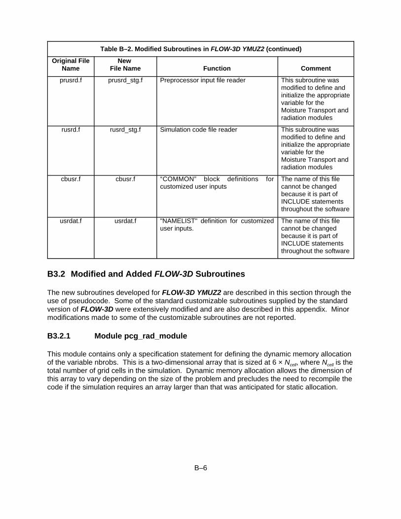
B–6

Table B–2. Modified Subroutines in FLOW-3D YMUZ2 (continued)

Original FileName

New File Name Function Comment

prusrd.f prusrd_stg.f Preprocessor input file reader This subroutine wasmodified to define andinitialize the appropriatevariable for theMoisture Transport andradiation modules

rusrd.f rusrd_stg.f Simulation code file reader This subroutine wasmodified to define andinitialize the appropriatevariable for theMoisture Transport andradiation modules

cbusr.f cbusr.f ?COMMON” block definitions forcustomized user inputs

The name of this filecannot be changedbecause it is part ofINCLUDE statementsthroughout the software

usrdat.f usrdat.f "NAMELIST" definition for customizeduser inputs.

The name of this filecannot be changedbecause it is part ofINCLUDE statementsthroughout the software

B3.2 Modified and Added FLOW-3D Subroutines

The new subroutines developed for FLOW-3D YMUZ2 are described in this section through theuse of pseudocode. Some of the standard customizable subroutines supplied by the standardversion of FLOW-3D were extensively modified and are also described in this appendix. Minormodifications made to some of the customizable subroutines are not reported.

B3.2.1 Module pcg_rad_module

This module contains only a specification statement for defining the dynamic memory allocationof the variable nbrobs. This is a two-dimensional array that is sized at 6 × Ncell, where Ncell is thetotal number of grid cells in the simulation. Dynamic memory allocation allows the dimension ofthis array to vary depending on the size of the problem and precludes the need to recompile thecode if the simulation requires an array larger than that was anticipated for static allocation.

B–7

B3.2.2 Subroutine nbr_init

This subroutine initializes and defines the array nbrobs. This subroutine is contained in the fileqsadd_pcg_rad.f.

! nbr_init pseudocodesubroutine nbr_init ! No arguments requirednbr_siz=size(vf) ! Get the total number of grid cells fr om the vf

! arrayAllocate the size of nbrobs to (6,nbr_siz) ! Set the size of nbrobs to the problem sizeInitialize nbrobs(m,ijk) = 0For nob = 1 to nobs

mincel=kvjk(nob) ! Get the range of cells with solid volume in themmaxcel ! for this obstacleijk=ijkvob(m)for m = mincel to maxcel

ijk = ijkvob(ijk) ! Get the cell index for this obstacle cell locationNeighbor cell indexes from mijk, pijkSet nbrobs(1,ipjk), nbrobs(2, imjk)….. ! Assign nbrobs for the neighbor cells nbrobs(2,ijpk), nbrobs(3,ijmk), ! Left direction of the cell to the right, etc.nbrobs(5,ijkp), nbrobs(6,ijkm) = nob

End loop for m = mincel to maxcelEnd loop for nob = 1 to nobsreturn

B3.2.3 Subroutine Teval

This subroutine computes the temperature corresponding to fluid volume-specific energy andfluid composition. The underlying theory for this subroutine is described in Appendix–A(Section A1.3). The code used here must be the reverse of the code used to compute the fluidenergy in subroutine e1cal so that there is a one-to-one correspondence between energy andtemperature for a specific combination of air concentration, water vapor concentration, andliquid water concentration. The teval object module contained in the standard FLOW-3D environment must be removed so that the object module created by compiling the code listedhere replaces the standard version. This subroutine is in the file named teval_stg.f todistinguish it from the standard version and as a reminder that a substitute version isbeing used.

function teval(ijk) ! Cell index ijk is the required argumentif (isvap .le. 0) stop ! If moisture model is not in use stop executionywv = sclr(ijk,isywv_stg) ! Get the vapor and liquid concentration ywl = sclr(ijk,isywl_stg) ! from the scalar arrayya = 1. – ywv – ywl ! Compute the air concentrationrhomix = rhof ! Use the nominal density defined for energy

! calc’steval = rhoe(ijk)/rhomix + ywl*hvvap_stg ! Temperature corresponding to this energy andteval = teval/(ya*cv1+ywv*cvvap_stg) ! compositionreturn

B–8

B3.2.4 Subroutine qsadd

This subroutine is the interface between the standard FLOW-3D code and the software for theMoisture Transport and Radiation Modules and is based on the sample code provided in thestandard FLOW-3D installation. This subroutine provides for the initialization requirements ofthese modules and calls the modules during FLOW-3D execution. This subroutine is in the filenamed qsadd_pcg_rad.f to distinguish it from the standard version.

subroutine qsadd ! No arguments are requiredif (nrsrf_stg and isvap_stg <= 0) return ! Return if phase change

and radiation are not activeif (cycle <=0) then ! Call initialization routines for first cycle

call nbr_init ! Initialize the nbrobs arrayif (nrsrf_stg .gt. 0) call rad_init ! Initialization for radiation calculationsif (isvap_stg .gt. 0) call pcg_init ! Initialization for Moisture Transport calculations

endifif (nrsrf_stg .gt. 0) call rad_calc ! Perform radiation calculationsif (isvap_stg .gt. 0) call pcg_calc ! Perform Moisture Transport calculationsreturn

B3.2.5 Subroutine pcg_init

There are several information items that are extracted from the FLOW-3D data arrays andstored. These procedures need to be performed only once at the start of the code executionand are separated from the Moisture Transport Module to make the execution more efficient. This subroutine provides for the initialization requirements of the Moisture Transport Moduleand is in the file named pcg_init_calc.f.

subroutine pcg_init ! No arguments are requiredmpcg=0 ! Initialize the surface cell indexnpsrf_stg=0 ! and surface counterDo 2000 nob =1 to nobs ! Loop over all the obstaclesif (imoist_stg(nob),ilqonly(nob) .ne. –nob) goto 2000 ! Skip if this obstacle is not ! moisture-active

npsrf_stg=npsrf_stg+1 ! Increment the surface counterrcobs_pcg(npsrf_stg) = rcobs(nob) ! Set the rho-c product for this surfaceimlpcg(stg(npsrf_stg) = ‘m’ or ‘l’ ! Define surface as infinite source/sinkif (ilqonly(nob) .eq. –nob) imlpcg_stg=’l’ ! or limited-liquidmincel=kajk(nob,nbl) ! Get the range of cells on the cell surfacemaxcel=kajk(nob+1,nbl)-1 ! surface ID array for this obstaclemmm=0 ! Initialize counter for moisture surface cellsfor m=mincel to maxcel ! Loop over all cells for this obstacle surface

ijk-ijkobs(m) ! Get the ijk index for this obstacle surf cellcall inijk ! Get the individual i,j,k

! get the neighbor indexes, imjk, ipjk, etcif (vf(ijk) .le. 1e-6)

skip to end of do m loop ! Skip if this cell is fully blocked by obstaclecompute vcell, vwall ! Total cell volume and solid-only volumemmm = mmm + 1 ! Increment the moisture surfacecell indexmpcg = mpcg + 1 ! Increment the moisture cell index limitif (mmm=1) kajk_pcg(npsrf_stg) = mpcg ! Assign limits for the moisture cell index

B–9

kajk_pcg(npsrf_stg+1) =- mpcg+1 ! ID array. kajk_pcg is analogous to kajkwaobs_pcg(mpcg) = waobs(m) ! Obstacle surface area formoisture surface cellsijk_pcg(mpcg) = ijk ! FLOW-3D cell index for this moisture surface

! cellijktw = ijk ! Assume this cell actually has the surface inside

! itIf this cell is fully open find fully ! Find the cell that has the wall obstacle and getclosed neighbor ! s index. This is used to get right wall temp laterijktw = index of neighbor that is fully closedvwall = solid volume of correct neighborwvobs_pcg(mpcg)=vwall ! Store the solid volume associated with this

! surfaceitw_pcg(mpcg) = ijktw ! FLOW-3D index for solid for with this surfaceEnd loop for m=mincel to maxcel

End Do 2000return

B3.2.6 Subroutine pcg_calc

This subroutine calculates the mass transfer at the wall and adjusts the wall surface celltemperatures to account for the heat of vaporization effects on the heat transfer in the walls. The basic theory for this process is described in Appendix A in Section A.1.4.1. The masstransfer at walls is effectively the source term in the species diffusion equation. The adjustmentof wall surface temperature is done here because there is no way for the user to directly assignthe heat source terms in the solid energy equation in FLOW-3D. The pcg_calc subroutine is inthe file named pcg_init_calc.f.

subroutine pcg_calc ! No arguments are requiredsclr(ijk,iii)=0for iii=isliq_stg, isrh_stg, uslq_stg, 7, 8 ! Initialize the bookkeeping scalars to zerofor ipsrf = 1 to npsrf_stg ! Loop over all moisture surfaces

Get mincel,maxcel from kajk_pcg ! Moisture surface cell ID limit this surfaceijk = ijk_pcg(m), ijktw-itw_pcg(m) ! FLOW-3D indexes this fluid and wall cell

call inijk ! Decode the i,j,k from Index ijkcompute imjk, ipjk, etc….. ! Get the neighbor cell indexesskip the rest of m loop if cell is fully blocked ! Trap possible error conditionvcell = fluid volume in cellvwall = wvobs_pcg(m) ! Get the solid volume and surface area for thissa = waobs_pcg(m) ! cell on this moisture surfaceif (tw(ijktw).le. 0) stop with error message ! If wall temp is non-existent, this is errortfinal=teval(ijk), tinit=tfinal ! Initialize cell temp according current energytwalli = tw(ijktw), twallf=twalli ! Initialize the wall temp to current valueyvacti=sclr(ijk,isvap_stg) ! Get current water mass fraction from previous sol’nnitr_moist=0 ! Initialize counter for wall calculationsIterate until temp is converged or count=25 ! Loop for finding wall temp and water mass fluxtnk = twallf or tfinal ! Set the temp for humidity properties accordinglycompute sat. mass fraction at fluid or wall tempcompute rhosat from mass

B–10

fractions and temps ! Bulk density at saturation compute delmmax Mass! required to bring entire cell to saturation

compute delmdif ! Mass entering cell if diffusion from wall is limitingdelm=min(delmmax,delmdif) ! Choose lower mass flowcompute new wall temp or fluid tempCheck if we’re out of condensed waterIf not converged on new temp, loop again for max of 25 iterationsdelmrat=delm/rho(ijk)/vcell ! New water mass as fractionsclr(ijk,isvap_stg)=(yvacti+delmrat)/(1+delmrat) ! New value of total water fractionsclr(ijk,isliq_stg)=sclr(ijk,isliq_stg)-delm/delt/sa ! Sum mass flux to get values from all wall neighborssclr(ijk,istlq_stg)=sclr(ijk,istlq_stg)-delm ! Total liquid accumulationUpdate the FLOW-3D arrays for wall temp or fluid temp End loop for m=mincel to maxce

End loop for ipsrf = 1 to npsrf_stgLoop over all real cells in flow domain that are not fully blockedyw=sclr(ijk,isvap_stg)nitr_moist2 = 0if (yw .le. yvsat .or. rhlim_stg .eq. ‘n’) skip calculations for RH shiftIterate until converged on new saturation temp for max of 25 iterationsnitr_moist2 = nitr_moist2 + 1ed0 = rhoe(ijk)/rhof ! Get the current value of mass-specific energyGet yvsat, saturation and mass fractioned1 = current value of energy ! The energy derivative depends on whetherd1edt = derivative of energy w.r.t. temp ! there is liquid presenttfinal=tfsave+vaprlx*(ed0-ed1)/de1dt ! Newton-Raphson equationIf not converged on new temp, loop again for max of 25 iterationsUpdate vapor, liquid fractions, cell temp ! Get new conditions that satisfy constant energy

End loop over all real cells in flow domain that are not fully blockedreturn

B3.2.7 Subroutine rad_init

There are several information items that are extracted from the FLOW-3D data arrays andstored for radiation surface areas and volumes. These procedures need to be performed onlyonce at the start of the code execution and are separated from the main part to make the codemore efficient. This subroutine also computes the radiation configuration factors and forms andthen inverts the heat flux coefficient matrix for use in computing the radiation heat fluxes. Theunderlying theory for this process is described in Appendix A, Section A.2.2. This subroutine isin the file named rad_init_calc.f.

subroutine rad_initLoop to set radl_rad(k_r,j_r) = 0 ! Initialize the heat flux coefficients

mrad = 0 ! Initialize the radiation cell indexFor irsrf = 1 to nrsrf_stg ! Transfer geometry limits to local variables

xl_srf = rad_stg(2,irsrf) ! for this loopxh_srf = rad_stg(3,irsrf)

etc. . . . . For all geometry limitsa_rad = 0 ! Initialize radiation surface areav_rad = 0 ! and volume for summing

B–11

For nob = 1 to nobs ! Loop over all obstacles to find the one if (rad_stg(1,irsrf) .eq. nob) then ! for this radiation surfacercobs_rad(irsrf)=rcobs(nob)mincel=kajk(nob,nbl) ! Get the range of cells for all the surface maxcel-kajk(nob+1,nbl) ! cells for this obstacle. kajk is a FLOW3Dmmm=0 ! Initialize radiation surface cell indexFor m=mincel to maxcel ! Loop over all FLOW3D cellsif (cell within geometry limits) then ! that make up the surface of this obstacle

vwall= compute obstacle volume if cell is empty, search the neighborcells for the obstacle volumemmm = mmm+1 ! Increment the radiation cell countersmrad = mrad + 1if (mmm=1) kajk_rad(irsrf)=mrad ! Set the min and max cellkajk_rad(irsrf+1)=mrad+1 ! indexes for this radiation surfacewaobs_rad(mrad) = waobs(m) ! Get the surface area for this cella_rad = a_rad+waobs(m) ! Sum to get the total surface area v_rad = v_rad + vwall ! Sum to get the total solid volume

! of surface cellsijk_rad(mrad)=ijktw ! Save the index for this rad

surface cellendifEnd loop for m=mincel to maxcel

End loop for nob=1 to nobssa_rad(irsrf) = a_rad ! Save the total area and volume sv_rad(irsrf) = v_rad ! radiation surface

End loop for irsrf=1 to nrsrfCompute the configuration factors

Find the minimum grid cell spacing for defining the ray tracing stepFor n=1 to nrsrf ! Loop through all the surfaces

cf_stg(n,n) ! Assume surface cannot see itselfmin_ns = kajk_rad(n) ! Get max and min indexes for max_ns = kajk_rad(n+1)-1 ! cells in radiation surface ‘n’For m= n+1 to nrsrf ! Loop over surfaces m>n

min_ms = kajk_rad(m) ! Get max and min indexes for max_ms = kajk_rad(m+1)-1 ! cells in radiation surface ‘m’sum = 0 ! Initialize the CF integral

For nn= min_ns to max_ns ! Loop over all cells in surface ‘n’ijk_m=ijk_rad(nn)

compute all local FLOW-3D indexes ! Get the cell surface area vector ! components

compute the dAn vector and magnitude ! and magnitude for element in ‘n’For mm=man_ms to max_ms ! Loop over all cells in surface ‘m’ijk_n=ijk_rad(nn)compute all local FLOW-3D indexes ! Get the cell surface area vector componentscompute the dAm vector and magnitude ! and magnitude for element in ‘n’

compute the vector Smncompute ns_ray, steps for ray tracingrqay = 1For nss=1 to ns_ray ! Trace along Smn to check for blockageif cell volume fraction <10-6, ray=0 ! Set factor to zero if blockedEnd loop for nss = 1 to ns_raycostnn = from dot product of dAn and Smncostmm = from dot product of dAm and Snm

B–12

denom=pi*Smn for 3-D ! Find the correct denominator for 2D or 3Ddenom = 2*Smn for 2-D problemsum=sum+ ray*costnn*costmm/denom ! Sum this contribution into the integralEnd of loop for mm=min_ms to max_msEnd of loop for nn=min_ns to max_nscf2d = 1 for 3-D ! Find the correct factor for 2-D or 3-Dcf2d = 1.delx or 1/dely or 1/delz for 2-D cf_stg(n,m) = cf2d*sum/sa_rad(n) ! compute the CF for n-mcf_stg(m,n) = cf_stg(n,m)*sa_rad(n)/sa_rad(m) ! Use reciprocity for CF of m-n

End of loop for m=n+1 to nrsrfEnd of loop for n=1 to nrsrfFor n=1 to nrsrf

For m=1 to nrsrf` ! Compute all the heat fluxCoefficientskdelta=0if (m=n) kdelta = 1radl_rad(m,n) = kdelta/eps_stg(m)-cf_stg(n,m)

*(1-eps_syg(m))/eps_stg(m)End of loop for m=1 to nrsrf

End of loop for n=1 to nrsrfcall matinv(radl_rad) ! Invert the matrix for calculations laterrecord the emissivities and configuration factors for reviewend of subroutine rad_init

B3.2.8 Subroutine matinv

This subroutine performs a matrix inversion by modified Gaussian elimination. This is astandard numerical technique and will not be described by pseudocode here. This subroutine iscalled only by rad_init.

B3.2.9 Subroutine rad_calcThis subroutine computes the radiation heat transfer rate from each radiation-active surface. The routine multiplies the inverted heat flux coefficient by the temperature array to computeradiation heat flux at each surface cell. The mathematical formulation of this subroutine isdescribed in Appendix A, Section A.2.1. The heat fluxes are used to adjust the surface celltemperatures to simulate the effects of the radiation heat flux as if it is a source or sink in theconduction energy equation for the affected cells. This subroutine is called only by qsadd.

subroutine rad_calcFor irsrf = 1 to nrsrf ! Find the average temp radiation surfaces

ta_rad=0mincel=kajk_rad(irsrf) ! Min and max cell indexes for this surfacemaxcel=kajk_rad(irsrf+1)-1for m=mincel to maxcelijk=ijk_rad(m) ! FLOW-3D ijk index for this cellcompute the local neighbor indexexta_rad=ta_rad+tw(ijk)*waobs_rad(m) ! Use area-weighted averageEnd loop for m=mincel to maxceltr_rad(irsrf)=ta_rad/sa_rad(irsrf)

end loop for irsrf=1 to nrsrf

For n=1 to nrsrf ! Compute the T^4 terms in the equationsradr_rad(n)=0 ! This is the RHS of model equation

B–13

for m=1 to nrsrf ! The H*T termskdelta=0if (m=n) kdelta = 1radr_rad(n) = radr(n)+(kdelta-cf_stg(n,m))*tr_rad(m)**4

end loop for m=1 to nrsrfend loop for n=1 to nrsrf

for n=1 to nrsrf !Compute the radiation heat fluxesqflx_rad(n)=0for m=1 to nrsrfqflx_rad(n)=qflx(n)-radl_rad(n,m)*radr(m) !Heat flux is positive away from surfaceend loop for m=1 to nrsrf

end loop for n=1 to nrsrf

prt_rad = 0 ! Record the heat fluxes forif (t .ge. tnext) then ! processing later

prt_rad=1tnext = tnext + pltdt ! Save on the FLOW-3D pltdt intervalwrite t, qflx_rad

for n=1 to nrsrf !Compute the delta-T for surfaces that are not fixed tempdtmp_rad=0if (rcobs_rad(n) .gt. 0) then

dtmp_rad = qflx_rad(n)*sa_rad(n)*delt/rcobs_rad(n)/sv_rad(n)

mincel=kajk_rad(n)maxcel=kajk_rad(n+1)-1 ! Apply the delta-T to all obstacle cells in this surfacefor m=mincel to maxcel

ijktw=ijk_rad(m)tw(ijktw) = tw(ijktw) + dtmp_rad

end loop for m=mincel to maxcelend loop for n=1 to nrsrf

end subroutine rad-calc

APPENDIX C

C–1

ADDITIONAL SAMPLE INPUT FILES

Appendix C represents the input files for the two-dimensional enclosed heat and mass trnsferproblem discussed in Chapter 4. This problem was investigated for four cases. The input filesfor the following cases are provided in this appendix. (1) Convection only(2) Convection with radiation(3) Convection with moisture transport

The input file has combined convection and radiation heat transfer with moisture transport andhas already been discussed in Section 4.2.4.

C1 INPUT FILE FOR CONVECTION-ONLY PROBLEM

Heat transfer in 2-D Sq. Box w/ natural convection, NO radiation, NO moisture Ra ~ 6000 for natural convection only Box is 0.1 m x 0.1 m long, Adiabatic at top and bottom, 20 W generated in left wall, 300 K at outer face of right wall. Both walls have k=1 w/(m*K), rcobs=1000*joule/(m^3*K) Moisture at left and right walls if modeled Radiation at left and right walls if modeled $xput

remark='units are SI',itb=0, remark='Sharp interface not required',ifvis=0, remark='Laminar',ifenrg=2, remark='Solve energy eq., first order',ifrho=1, remark='Temp. dependent density',gz=-9.8e-03, remark='Gravity',ipdis=1, remark='Hydrostatic prfessure distribution in z-direction',ihtc=2, remark='Evaluate heat transfer with solid conduction',iwsh=1, remark='Wall shear active',delt=1.e-4, remark='',twfin=4000., remark='',rmrhoe=0., remark='Density diffusion term coefficient',rmrho=0., remark='Energy diffusion term coefficient', remark=' RMRHO, RMRHOE = 1 REQUIRED FOR VAPOR TRANSPORT MODEL ', iusrd=1,

$end

$limits $end

$propsunits='si', rhof=1.1687, remark='Bulk nominal density at 310 K for energy equation', mu1=2.e-05, remark='Bulk nominal dynamic viscosity density for momentum equation', cv1=717., remark='Const. Vol. Specific heat of dry air', thc1=0.026, remark='Bulk nominal thermal conductivity for energy equation', thexf1=0.003226, remark='Approximate thermal expansion coefficient',

C–2

tstar = 300., remark='Reference temperature for thermal expansion coefficient', remark='THEXF1, TSTAR not needed for vapor tranport model', remark='but are used in some parts of code to set up simualtion',

$end

$scalar remark='Water vapor scalars not used for this problem but need to be defined to use the ', remark=' radiation and water transport modules together', remark='Scalar 1 is the diffusing/advecting water', remark='Scalar 2 (non-diffusing) is for storing the surface phase change flux values', remark='Scalar 3 (non-diffusing) is for storing the relative humidity values', remark='Scalar 4 (non-diffusing) is for storing the net surface liquid accumulation', remark='Scalar 5 (non-diffusing) is for storing the vapor water concentration', remark='Scalar 6 (non-diffusing) is for storing the liquid water (mist) concentration', remark='Scalar 7 (non-diffusing) is for storing the calculation iterations for the', remark=' wall mass flux', remark='Scalar 8 (non-diffusing) is for storing the calculation iterations for the', remark=' mist phase change in the fluid interior', remark='Scalars 7 and 8 are helpful in tuning the value of vaprlx if necessary', nsc=8, isclr(1)=3, cmsc(1)=0.26e-04, scltit(1)='Tot.Water', rmsc=0., isclr(2)=0, cmsc(2)=0., scltit(2)='Liq.Flux', isclr(3)=0, cmsc(3)=0., scltit(3)='Rel.Hum', isclr(4)=0, cmsc(4)=0., scltit(4)='Net.Liq', isclr(5)=0, cmsc(5)=0., scltit(5)='Vap.Wat', isclr(6)=0, cmsc(6)=0., scltit(6)='Liq.Wat', isclr(7)=0, cmsc(7)=0., scltit(7)='Itr.Wall', isclr(8)=0, cmsc(8)=0., scltit(8)='Itr.Mesh', $end

$bcdata wl=1, remark='Symmetry at left to make all the heat go into the inner face', wr=2, remark='Constant temperature wall at right', tbc(2)=300., wf=1, wbk=1, remark=' Symmetry at front and back', wb=2, remark=' Insulated wall', wt=2, remark=' Insulated wall',

$end

$mesh px(1) =-0.025, py(1) =0.0, pz(1) = 0.0, px(2) = 0.0, py(2) =1., pz(2) = 0.1, px(3) = 0.1, px(4) = 0.125, nxcell(1)=5, nxcell(2)=20, nxcell(3)=5, nxcelt= 30, nycelt=1, nzcelt=30,

$end

$obs avrck=-3.1, nobs = 2, tobs(1)=0., tobs(2)=1000., remark='Obstacle 1. Left channel wall. Total heat output 50W',

C–3

xl(1)=-0.025, xh(1)=0., kobs(1)= 1., rcobs(1)=10000., twobs(1,1)=300., pobs(1,1)=20., pobs(2,1)=20., remark='Obstacle 2. Right channel wall. Conduction to constant temp', xl(2)=0.1, xh(2)=0.125, kobs(2)= 1., rcobs(2)=10000., twobs(1,2)=300., $end

$fl remark=' No vapor in fluid', sclri(1)=0.0, sclri(5)=0.0, sclri(6)=0.0, presi=101325.,

$end

$bf $end $temp ntmp=1, tempi=300., $end $motn $end $grafic $end $parts $end $usrdat

istwtf_stg='tw', remark='Energy for phase change comes from wall', isvap_stg = 1, remark='Define scalar index for water concentration DO NOT CHANGE', isliq_stg = 2, remark='Define scalar index for liquid flux DO NOT CHANGE', isrh_stg = 3, remark='Define scalar index for rel. hum. DO NOT CHANGE', istlq_stg = 4, remark='Define scalar index for tot.liq. accum. DO NOT CHANGE', isywv_stg = 5, remark='Define scalar index for vapor water DO NOT CHANGE', isywl_stg = 6, remark='Define scalar index for liquid water (mist) DO NOT CHANGE', hvvap_stg=2304900., remark='Heat of vaporization', cvvap_stg=1370., remark='Water vapor specific heat (const. vol.)', cvliq_stg=4186., remark='Water liquid specific heat (const. vol.)', rvap_stg=416., remark='Gas constant for water vapor', rgas_stg=289., remark='Gas constant for air', vaprlx_stg=0.8, remark='Relaxation factor for phase change iterations', rhlim_stg='y', remark='Limit rel humidity to 100 percent',

$end

C2 INPUT FILE FOR CONVECTION WITH RADIATION

Heat transfer in 2-D Sq. Box w/ natural convection, radiation, NO moisture Ra ~ 6000 for natural convection only Box is 0.1 m x 0.1 m long, Adiabatic at top and bottom, 20 W generated in left wall, 300 K at outer face of right wall.

C–4

Both walls have k=1 w/(m*K), rcobs=1000*joule/(m^3*K) Moisture at left and right walls if modeled Radiation at left and right walls if modeled

$xput remark='units are SI', itb=0, remark='Sharp interface not required', ifvis=0, remark='Laminar', ifenrg=2, remark='Solve energy eq., first order', ifrho=1, remark='Temp. dependent density', gz=-9.8e-03, remark='Gravity', ipdis=1, remark='Hydrostatic prfessure distribution in z-direction', ihtc=2, remark='Evaluate heat transfer with solid conduction', iwsh=1, remark='Wall shear active', delt=1.e-4, remark='', twfin=4000., remark='', rmrhoe=0., remark='Density diffusion term coefficient', rmrho=0., remark='Energy diffusion term coefficient', remark=' RMRHO, RMRHOE = 1 REQUIRED FOR VAPOR TRANSPORT MODEL ', iusrd=1, $end

$limits $end

$props units='si', rhof=1.1687, remark='Bulk nominal density at 310 K for energy equation', mu1=2.e-05, remark='Bulk nominal dynamic viscosity density for momentum equation', cv1=717., remark='Const. Vol. Specific heat of dry air', thc1=0.026, remark='Bulk nominal thermal conductivity for energy equation', thexf1=0.003226, remark='Approximate thermal expansion coefficient', tstar = 300., remark='Reference temperature for thermal expansion coefficient', remark='THEXF1, TSTAR not needed for vapor transport model', remark='but are used in some parts of code to set up simulation', $end

$scalar remark='Water vapor scalars not used for this problem but need to be defined to use the ', remark=' radiation and water transport modules together', remark='Scalar 1 is the diffusing/advecting water', remark='Scalar 2 (non-diffusing) is for storing the surface phase change flux values', remark='Scalar 3 (non-diffusing) is for storing the relative humidity values', remark='Scalar 4 (non-diffusing) is for storing the net surface liquid accumulation', remark='Scalar 5 (non-diffusing) is for storing the vapor water concentration', remark='Scalar 6 (non-diffusing) is for storing the liquid water (mist) concentration', remark='Scalar 7 (non-diffusing) is for storing the calculation iterations for the', remark=' wall mass flux', remark='Scalar 8 (non-diffusing) is for storing the calculation iterations for the', remark=' mist pahse change in the fluid interior', remark='Scalars 7 and 8 are helpful in tuning the value of vaprlx if necessary', nsc=8, isclr(1)=3, cmsc(1)=0.26e-04, scltit(1)='Tot.Water', rmsc=0., isclr(2)=0, cmsc(2)=0., scltit(2)='Liq.Flux', isclr(3)=0, cmsc(3)=0., scltit(3)='Rel.Hum',

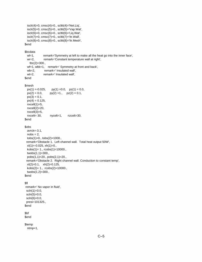
C–5

isclr(4)=0, cmsc(4)=0., scltit(4)='Net.Liq', isclr(5)=0, cmsc(5)=0., scltit(5)='Vap.Wat', isclr(6)=0, cmsc(6)=0., scltit(6)='Liq.Wat', isclr(7)=0, cmsc(7)=0., scltit(7)='Itr.Wall', isclr(8)=0, cmsc(8)=0., scltit(8)='Itr.Mesh', $end


$mesh px(1) =-0.025, py(1) =0.0, pz(1) = 0.0, px(2) = 0.0, py(2) =1., pz(2) = 0.1, px(3) = 0.1, px(4) = 0.125, nxcell(1)=5, nxcell(2)=20, nxcell(3)=5, nxcelt= 30, nycelt=1, nzcelt=30, $end


$fl remark=' No vapor in fluid', sclri(1)=0.0, sclri(5)=0.0, sclri(6)=0.0, presi=101325., $end

$bf $end

$temp ntmp=1,

C–6

tempi=300., $end

$motn $end

$grafic $end

$parts $end

$usrdat

nrsrf_stg=2,

eps_stg(1) = .9, rad_stg(1,1) = 1., rad_stg(2,1) =-0.004, rad_stg(3,1) = 0.004, rad_stg(4,1) =-1., rad_stg(5,1) = 2., rad_stg(6,1) = 0.0, rad_stg(7,1) = 0.2,

eps_stg(2) = .9, rad_stg(1,2) = 2., rad_stg(2,2) = 0.096, rad_stg(3,2) = 0.104, rad_stg(4,2) =-1., rad_stg(5,2) = 2., rad_stg(6,2) = 0.0, rad_stg(7,2) = 0.2,

iusrcf_stg=0,

istwtf_stg='tw', remark='Energy for phase change comes from wall',

isvap_stg = 1, remark='Define scalar index for water concentration DO NOT CHANGE', isliq_stg = 2, remark='Define scalar index for liquid flux DO NOT CHANGE', isrh_stg = 3, remark='Define scalar index for rel. hum. DO NOT CHANGE', istlq_stg = 4, remark='Define scalar index for tot.liq. accum. DO NOT CHANGE', isywv_stg = 5, remark='Define scalar index for vapor water DO NOT CHANGE', isywl_stg = 6, remark='Define scalar index for liquid water (mist) DO NOT CHANGE', hvvap_stg=2304900., remark='Heat of vaporization', cvvap_stg=1370., remark='Water vapor specific heat (const. vol.)', cvliq_stg=4186., remark='Water liquid specific heat (const. vol.)', rvap_stg=416., remark='Gas constant for water vapor', rgas_stg=289., remark='Gas constant for air', vaprlx_stg=0.8, remark='Relaxation factor for phase change iterations', rhlim_stg='y', remark='Limit rel humidity to 100 percent',

$end

C3 INPUT FILE FOR CONVECTION WITH MOISTURE TRANSPORT

Heat transfer in 2-D Sq. Box w/ natural convection, NO radiation, moisture Ra ~ 6000 for natural convection only Box is 0.1 m x 0.1 m long, Adiabatic at top and bottom,

C–7

20 W generated in left wall, 300 K at outer face of right wall. Both walls have k=1 w/(m*K), rcobs=1000*joule/(m^3*K) Moisture at left and right walls if modeled Radiation at left and right walls if modeled

$xput remark='units are SI', itb=0, remark='Sharp interface not required', ifvis=0, remark='Laminar', ifenrg=2, remark='Solve energy eq., first order', ifrho=1, remark='Temp. dependent density', gz=-9.8e-03, remark='Gravity', ipdis=1, remark='Hydrostatic prfessure distribution in z-direction', ihtc=2, remark='Evaluate heat transfer with solid conduction', iwsh=1, remark='Wall shear active', delt=1.e-4, remark='', twfin=4000., remark='', rmrhoe=1., remark='Density diffusion term coefficient', rmrho=1., remark='Energy diffusion term coefficient', remark=' RMRHO, RMRHOE REQUIRED FOR VAPOR TRANSPORT MODEL ', iusrd=1, $end

$limits $end

$props units='si', rhof=1.1687, remark='Bulk nominal density at 310 K for energy equation', mu1=2.e-05, remark='Bulk nominal dynamic viscosity density for momentum equation', cv1=717., remark='Const. Vol. Specific heat of dry air', thc1=0.026, remark='Bulk nominal thermal conductivity for energy equation', thexf1=0.003226, remark='Approximate thermal expansion coefficient', tstar = 300., remark='Reference temperature for thermal expansion coefficient', remark='THEXF1, TSTAR not needed for vapor transport model', remark='but are used in some parts of code to set up simulation', $end

$scalar remark='Water vapor scalars not used for this problem but need to be defined to use the ', remark=' radiation and water transport modules together', remark='Scalar 1 is the diffusing/advecting water', remark='Scalar 2 (non-diffusing) is for storing the surface phase change flux values', remark='Scalar 3 (non-diffusing) is for storing the relative humidity values', remark='Scalar 4 (non-diffusing) is for storing the net surface liquid accumulation', remark='Scalar 5 (non-diffusing) is for storing the vapor water concentration', remark='Scalar 6 (non-diffusing) is for storing the liquid water (mist) concentration', remark='Scalar 7 (non-diffusing) is for storing the calculation iterations for the', remark=' wall mass flux', remark='Scalar 8 (non-diffusing) is for storing the calculation iterations for the', remark=' mist pahse change in the fluid interior', remark='Scalars 7 and 8 are helpful in tuning the value of vaprlx if necessary', nsc=8, isclr(1)=3, cmsc(1)=0.26e-04, scltit(1)='Tot.Water', rmsc=0.,

C–8

isclr(2)=0, cmsc(2)=0., scltit(2)='Liq.Flux', isclr(3)=0, cmsc(3)=0., scltit(3)='Rel.Hum', isclr(4)=0, cmsc(4)=0., scltit(4)='Net.Liq', isclr(5)=0, cmsc(5)=0., scltit(5)='Vap.Wat', isclr(6)=0, cmsc(6)=0., scltit(6)='Liq.Wat', isclr(7)=0, cmsc(7)=0., scltit(7)='Itr.Wall', isclr(8)=0, cmsc(8)=0., scltit(8)='Itr.Mesh', $end


$mesh px(1) =-0.025, py(1) =0.0, pz(1) = 0.0, px(2) = 0.0, py(2) =1., pz(2) = 0.1, px(3) = 0.1, px(4) = 0.125, nxcell(1)=5, nxcell(2)=20, nxcell(3)=5, nxcelt= 30, nycelt=1, nzcelt=30, $end


$fl remark=' No vapor in fluid', sclri(1)=0.0, sclri(5)=0.0, sclri(6)=0.0, presi=101325., $end

$bf $end

C–9

$temp ntmp=1, tempi=300., $end

$motn $end

$grafic $end

$parts $end

$usrdat

istwtf_stg='tw', remark='Energy for phase change comes from wall', imoist_stg(1)=-1, imoist_stg(2)=-2, isvap_stg = 1, remark='Define scalar index for water concentration DO NOT CHANGE', isliq_stg = 2, remark='Define scalar index for liquid flux DO NOT CHANGE', isrh_stg = 3, remark='Define scalar index for rel. hum. DO NOT CHANGE', istlq_stg = 4, remark='Define scalar index for tot.liq. accum. DO NOT CHANGE', isywv_stg = 5, remark='Define scalar index for vapor water DO NOT CHANGE', isywl_stg = 6, remark='Define scalar index for liquid water (mist) DO NOT CHANGE', hvvap_stg=2304900., remark='Heat of vaporization', cvvap_stg=1370., remark='Water vapor specific heat (const. vol.)', cvliq_stg=4186., remark='Water liquid specific heat (const. vol.)', rvap_stg=416., remark='Gas constant for water vapor', rgas_stg=289., remark='Gas constant for air', vaprlx_stg=0.8, remark='Relaxation factor for phase change iterations', rhlim_stg='y', remark='Limit rel humidity to 100 percent',

$end

a center of excellence in earth sciences and engineeringm · analyses and codes: the flow-3d®...

Documents