a central limit theorem for punctuated equilibrium
TRANSCRIPT

Full Terms & Conditions of access and use can be found athttps://www.tandfonline.com/action/journalInformation?journalCode=lstm20
Stochastic Models
ISSN: 1532-6349 (Print) 1532-4214 (Online) Journal homepage: https://www.tandfonline.com/loi/lstm20
A Central Limit Theorem for punctuatedequilibrium
K. Bartoszek
To cite this article: K. Bartoszek (2020): A Central Limit Theorem for punctuated equilibrium,Stochastic Models, DOI: 10.1080/15326349.2020.1752242
To link to this article: https://doi.org/10.1080/15326349.2020.1752242
© 2020 The Author(s). Published withlicense by Taylor & Francis Group, LLC
Published online: 05 May 2020.
Submit your article to this journal
Article views: 142
View related articles
View Crossmark data
A Central Limit Theorem for punctuated equilibrium
K. Bartoszek
Department of Computer and Information Science, Link€oping University, Link€oping, Sweden
ABSTRACTCurrent evolutionary biology models usually assume that aphenotype undergoes gradual change. This is in stark contrastto biological intuition, which indicates that change can alsobe punctuated—the phenotype can jump. Such a jump couldespecially occur at speciation, i.e., dramatic change occurs thatdrives the species apart. Here we derive a Central LimitTheorem for punctuated equilibrium. We show that, if adapta-tion is fast, for weak convergence to normality to hold, thevariability in the occurrence of change has to disappearwith time.
ARTICLE HISTORYReceived 5 January 2017Accepted 2 April 2020
KEYWORDSBranching diffusion process;conditioned branchingprocess; Central LimitTheorem; L�evy process;punctuated equilibrium;Yule–Ornstein–Uhlenbeckwith jumps process
AMS SUBJECTCLASSIFICATION60F05; 60J70; 60J85;62P10; 92B99
1. Introduction
A long–standing debate in evolutionary biology is whether changes takeplace at times of speciation (punctuated equilibrium Eldredge andGould[28], Gould and Eldredge[32] or gradually over time (phyletic gradual-ism, see references in Eldredge and Gould[28]. Phyletic gradualism is in linewith Darwin’s original envisioning of evolution (Eldredge and Gould[28]).On the other hand, the theory of punctuated equilibrium was an answer towhat fossil data was indicating (Eldredge and Gould[28], Gould andEldredge[31,32]). A complete unbroken fossil series was rarely observed,rather distinct forms separated by long periods of stability (Eldredge andGould[28]). Darwin saw “the fossil record more as an embarrassment thanas an aid to his theory” (Eldredge and Gould[28]) in the discussions withFalconer at the birth of the theory of evolution. Evolution with jumps wasproposed under the name “quantum evolution” (Simpson[50]) to the scien-tific community. However, only later (Eldredge and Gould[28]) was punctu-ated equilibrium re–introduced into contemporary mainstream
CONTACT K. Bartoszek [email protected], [email protected] Department of Computer andInformation Science, Link€oping University, 581 83 Link€oping, Sweden.� 2020 The Author(s). Published with license by Taylor & Francis Group, LLCThis is an Open Access article distributed under the terms of the Creative Commons Attribution License (http://creativecommons.org/licenses/by/4.0/), which permits unrestricted use, distribution, and reproduction in any medium, providedthe original work is properly cited.
STOCHASTIC MODELShttps://doi.org/10.1080/15326349.2020.1752242

evolutionary theory. Mathematical modeling of punctuated evolution onphylogenetic trees seems to be still in its infancy (but see Bokma[19,21,22],Mattila and Bokma[37], Mooers and Schluter[42], Mooers et al.[43]). Themain reason is that we do not seem to have sufficient understanding of thestochastic properties of these models. An attempt was made in this direc-tion (Bartoszek[10])—to derive the tips’ mean, variance, covariance andinterspecies correlation for a branching Ornstein–Uhlenbeck (OU) processwith jumps at speciation, alongside a way of quantitatively assessing theeffect of both types of evolution. Very recently Bastide et al.[15] consideredthe problem from a statistical point of view and proposed anExpectation–Maximization algorithm for a phylogenetic Brownian motionwith jumps model and an OU with jumps in the drift function model. Thiswork is very important to indicate as it includes estimation software for apunctuated equilibrium model, something not readily available earlier.Bitseki Penda et al.[18] also recently looked into estimation procedures forbifurcating Markov chains.Combining jumps with an OU process is attractive from a biological
point of view. It is consistent with the original motivation behind punctu-ated equilibrium. At branching, dramatic events occur that drive speciesapart. But then stasis between these jumps does not mean that no changetakes place, rather that during it “fluctuations of little or no accumulatedconsequence” occur (Gould and Eldredge[32]). The OU process fits into thisidea because if the adaptation rate is large enough, then the process reachesstationarity very quickly and oscillates around the optimal state. This thencan be interpreted as stasis between the jumps—the small fluctuations.Mayr[38] supports this sort of reasoning by hypothesizing that “The furtherremoved in time a species from the original speciation event that originatedit, the more its genotype will have become stabilized and the more it islikely to resist change.” It should perhaps be noted at this point, that aReviewer pointed out that the modeling approach presented in this work isnot the same as the “classical view of punctuated equilibrium”. One wouldexpect the jump to take place in the direction of the optimum trait value.However, here at speciation the jump is allowed to take place in any direc-tion, also away from the optimum. Then, after the jump, a relaxationperiod occurs and the trait is allowed to evolve back to the optimum. Sucha view on the jumps is similar to e.g. Bokma’s[19,21] modeling approach,however, there the Brownian motion (BM) process was considered so nooptimum parameter was present. All the presented here results, concernthe balance between the relaxation phenomena and the jumps’ magnitudesand chances of occurring. One way of maybe thinking about jumps goingagainst the optimum, is that at the speciation event a short–lived (as after-words evolution goes again in the direction of the previous optimum),
2 K. BARTOSZEK

random environmental niche appeared that allowed part of the species’population to break–off and form a new species. However, to make thisany more formal one would have to link it with models for the environ-ment, fitness and trait dependent speciation, which is beyond the scope ofthis paper.In this work we build up on previous results (Bartoszek[10], Bartoszek and
Sagitov[12]) and study in detail the asymptotic behavior of the average of thetip values of a branching OU process, with jumps at speciation points, evolv-ing on a pure birth tree. To the best of our knowledge the work here is oneof the first to consider the effect of jumps on a branching OU process in aphylogenetic context (but also look at Bastide et al.[15]). It is possible thatsome of the results could be special subcases of general results on branchingMarkov processes (e.g. Abraham and Delmas[1], Bansaye et al.[8], Cloez andHairer[24], Marguet[36], Ren et al.[46–48]). However, these studies use a veryheavy functional analysis apparatus, which unlike the direct one here, couldbe difficult for the applied reader. Bansaye et al.[8], Guyon[33], Bitseki Pendaet al.[17]’s works are worth pointing out as they connect their results onbifurcating Markov processes with biological settings where branching phe-nomena are applicable, e.g., cell growth.In the work here we can observe the (well known) competition between
the tree’s speciation and OU’s adaptation (drift) rates, resulting in a phasetransition when the latter is half the former (the same as in the no jumpscase Adamczak and Miło�s[2,3], An�e et al.[4], Bartoszek and Sagitov[12]). Weshow here that if variability in jump occurrences disappears with time orthe model is in the critical regime (plus a bound assumption on the jumps’magnitude and chances of occurring), then the contemporary sample meanwill be asymptotically normally distributed. Otherwise the weak limit canbe characterized as a “normal distribution with a random variance”. Suchprobabilistic characterizations are important as tools for punctuated phylo-genetic models are starting to be developed (e.g., Bastide et al.[15]). This ispartially due to an uncertainty of what is estimable, especially whether thecontribution of gradual and punctuated change may be disentangled (butBokma[22] indicates that they should be distinguishable). Large sample sizedistributional approximations will allow for choosing seeds for numericalmaximum likelihood procedures and sanity checks if the results of numer-ical procedures make sense. For example in the one–dimensional OU caseit is known that (for a Yule tree) the sample average is a consistent estima-tor of the long term mean and the sample variance of the OU process’ sta-tionary variance (Bartoszek and Sagitov[12]). In the BM (Yule tree) case onecan have a consistent estimator of the diffusion coefficient.[13] Hence, fromthese sample statistics one can construct starting values for numerical esti-mation procedures (as e.g. mvSLOUCH does now[14]).
STOCHASTIC MODELS 3
Often a key ingredient in studying branching Markov processes is a“Many–to–One” formula—the law of the trait of an uniformly sampledindividual in an “average” population (e.g. Marguet[36]). The approach inthis paper is that on the one hand we condition on the population size, n,but then to obtain the law (and its limit) of the contemporary population,we consider moments of uniformly sampled species and the covariancebetween a uniformly sampled pair of species.The strategy to study the limit behavior is to first condition on a realiza-
tion of the Yule tree and jump pattern (on which branches after speciationdid the jump take place). This is, as conditional on the phylogeny andjump locations, the collection of the contemporary tips’ trait values willhave a multivariate normal distribution, and hence their sample averagewill be normally distributed. We are able to represent (under the aboveconditioning) the variance of the sample average in terms of transforma-tions of the number of speciation events on randomly selected lineage, timeto coalescent of randomly selected pair of tips and the number of commonspeciation events for a randomly selected pair of tips. We consider the con-ditional (on the tree and jump pattern) expectation of these transforma-tions and then look at the rate of decay to 0 of the variances of theseconditional expectations. If this rate of decay is fast enough, then they willconverge to a constant and the normality of an appropriately scaled averageof tips species will be retained in the limit. Very briefly this rate of decaydepends on how the product of the probability and variance of the jumpbehaves along the nodes of the tree. We do not necessarily assume (as pre-viously by Bartoszek[10]) that the jumps are homogeneous on thewhole tree.First, in Section 2 we provide a series of formal definitions that
introduce key random variables associated with the phylogeny that arenecessary for this study. Afterwords, in Section 3 we introduce the con-sidered probabilistic model and the concepts from Section 2 in a moreintuitive manner. Then, in Section 4 we present the main results.Section 5 is devoted to a series of technical convergence lemmata thatcharacterize the speed of decay of the effect of jumps on the varianceand covariance of tip species. Finally, in Section 6 we calculate the firsttwo moments of a scaled sample average, introduce a particular randomvariable related to the model and put this together with the previousconvergence lemmata to prove the Central Limit Theorems (CLTs) ofthis paper. It should be acknowledged at this point that in the originalarXiv preprint of this paper the convergence to normality results werestated in an incomplete manner. In particular the limiting normality inthe critical regime was not described correctly. The current character-ization was noticed during the collaboration with Torkel Erhardsson[11]
4 K. BARTOSZEK
and more details on the previous mischaracterization can be found inRemark 4.7.
2. Notation
We first introduce two separate labellings for the tip and internal nodes ofthe tree. Let the origin of the tree have label “0”. Next we label from “1” to“n – 1” the internal nodes of the tree in their temporal order of appear-ance. The root is “1”, the node corresponding to the second speciationevent is “2” and so on. We label the tips of the tree from “1” to “n” in anarbitrary fashion. This double usage of the numbers “1” to “n – 1” doesnot generate any confusion as it will always be clear whether one refers toa tip or internal node.
Definition 2.1.
NTipðtÞ ¼ set of tip nodes at time tf g
Definition 2.2.
UðnÞ ¼ inf t � 0 : jNTipðtÞj ¼ n� �
,
where jAj denotes the cardinality of set A.
Definition 2.3. For i 2 NTipðUðnÞÞ,!ði, nÞ : number of nodes on the path from the root
ðinternal node 1, including itÞ to tip node i
Definition 2.4. For i 2 NTipðUðnÞÞ, define the finite sequence of length
!ði, nÞ as
Iði, nÞ ¼ Iði, nÞj : Iði, nÞj is a node on the root to tip node i path and�Iði, nÞj < Iði, nÞk for 1 � j < k � !ði, nÞ
�!ði, nÞ
j¼1
Definition 2.5. For i 2 NTipðUðnÞÞ and r 2 1, :::, n� 1f g, let 1ði, nÞr be a bin-ary random variable such that
1ði, nÞr ¼ 1 iff r 2 Iði, nÞ,
where the 2 should be understood in the natural way that there exists a
position j in the sequence Iði, nÞ s.t. Iði, nÞj ¼ r:
STOCHASTIC MODELS 5
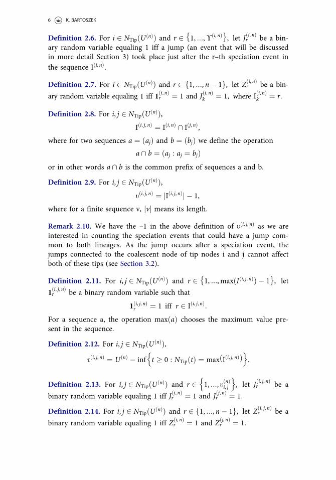
Definition 2.6. For i 2 NTipðUðnÞÞ and r 2 1, :::,!ði, nÞ� �, let Jði, nÞr be a bin-
ary random variable equaling 1 iff a jump (an event that will be discussedin more detail Section 3) took place just after the r–th speciation event inthe sequence Iði, nÞ:
Definition 2.7. For i 2 NTipðUðnÞÞ and r 2 1, :::, n� 1f g, let Zði, nÞr be a bin-
ary random variable equaling 1 iff 1ði, nÞr ¼ 1 and Jði, nÞk ¼ 1, where Iði, nÞk ¼ r:
Definition 2.8. For i, j 2 NTipðUðnÞÞ,Iði, j, nÞ ¼ Iði, nÞ \ Iðj, nÞ,
where for two sequences a ¼ ðajÞ and b ¼ ðbjÞ we define the operation
a \ b ¼ ðaj : aj ¼ bjÞor in other words a \ b is the common prefix of sequences a and b.
Definition 2.9. For i, j 2 NTipðUðnÞÞ,tði, j, nÞ ¼ jIði, j, nÞj � 1,
where for a finite sequence v, jvj means its length.
Remark 2.10. We have the –1 in the above definition of tði, j, nÞ as we areinterested in counting the speciation events that could have a jump com-mon to both lineages. As the jump occurs after a speciation event, thejumps connected to the coalescent node of tip nodes i and j cannot affectboth of these tips (see Section 3.2).
Definition 2.11. For i, j 2 NTipðUðnÞÞ and r 2 1, :::, maxðIði, j, nÞÞ � 1� �
, let
1ði, j, nÞr be a binary random variable such that
1ði, j, nÞr ¼ 1 iff r 2 Iði, j, nÞ:
For a sequence a, the operation maxðaÞ chooses the maximum value pre-sent in the sequence.
Definition 2.12. For i, j 2 NTipðUðnÞÞ,sði, j, nÞ ¼ UðnÞ � inf t � 0 : NTipðtÞ ¼ max Iði, j, nÞð Þ
n o:
Definition 2.13. For i, j 2 NTipðUðnÞÞ and r 2 1, :::, tðnÞi, j
n o, let Jði, j, nÞr be a
binary random variable equaling 1 iff Jði, nÞr ¼ 1 and Jðj, nÞr ¼ 1:
Definition 2.14. For i, j 2 NTipðUðnÞÞ and r 2 1, :::, n� 1f g, let Zði, j, nÞr be a
binary random variable equaling 1 iff Zði, nÞr ¼ 1 and Zðj, nÞ
r ¼ 1:
6 K. BARTOSZEK
Definition 2.15. Let R be uniformly distributed on 1, :::, nf g and (R, K) beuniformly distributed on the set of ordered pairs drawn from 1, :::, nf g(i.e., Prob R,Kð Þ ¼ r, kð Þ� � ¼ n
2
� �1
, for 1 � r < k � n)
s nð Þ ¼ s R,K, nð Þ, ! nð Þ ¼ ! R, nð Þ, t nð Þ ¼ t R,K, nð Þ, I nð Þ ¼ I R, nð Þ,
~Inð Þ ¼ I R,K, nð Þ, 1i ¼ 1 R, nð Þ
i , ~1i ¼1 R,K, nð Þi , Ji ¼ J R, nð Þ
i , ~J i ¼ J R,K, nð Þi ,
Zi ¼ Z R, nð Þi , ~Zi ¼ Z R,K, nð Þ
i :
Some of the variables defined in Defn. 2.15 are illustrated in Figures 1, 5and further described in the captions. It might be also useful to refer toBartoszek[10], especially Figure A.8, therein.
Remark 2.16. For the sequences I nð Þ, I r, nð Þ, I R, nð Þ,~Inð Þ, I r, k, nð Þ, I R,K, nð Þ the i–th
element is naturally indicated as I nð Þi , I
r, nð Þi , I R, nð Þ
i , ~Inð Þi , I r, k, nð Þ
i , I R,K, nð Þi
respectively.
Remark 2.17. We drop the n in the superscript for the random variables
1i, ~1i, Ji, ~J i, Zi and ~Zi as their distribution will not depend on n (seeLemma 3.1 Section 3). In fact, in principle, there will be no need to distin-guish between the version with and without the tilde. However, such a dis-tinction will make it more clear to what one is referring to in thesubsequent derivations in this work.
3. A model for punctuated stabilizing selection
3.1. Phenotype model
Stochastic differential equations (SDEs) are today the standard language tomodel continuous traits evolving on a phylogenetic tree. The generalframework is that of a diffusion process
dX tð Þ ¼ l t,X tð Þð Þdt þ radBt: (1)
The trait, X tð Þ 2 R, follows Eq. (1) along each branch of the tree (withpossibly branch specific parameters). At speciation times this processdivides into two processes evolving independently from that point. A work-horse of contemporary phylogenetic comparative methods (PCMs) is theOU process
dX tð Þ ¼ �a X tð Þ � hð Þdt þ radBt, (2)
where sometimes the parameters a, h, ra are allowed to vary over the tree(see e.g. Bartoszek et al.[14], Beaulieu et al.[16], Butler and King[23],
STOCHASTIC MODELS 7
Hansen[34], Mitov et al.[40,41]). Without loss of generality, for the purposeof the results here, we could have taken h¼ 0. However, we choose toretain the parameter for consistency with previous literature. In this workwe keep all the parameters (a, h, ra) identical over the whole tree.The probabilistic properties (e.g. de Saporta and Yao[7]) and statistical
procedures (e.g., Azaïs et al.[6]) for processes with jumps have of coursebeen developed. In the phylogenetic context there have been a few attemptsto go beyond the diffusion framework into L�evy process, including Laplacemotion, (Bartoszek[9], Duchen et al.[26], Landis et al.[35]) and jumps at spe-ciation points (Bartoszek[10], Bastide et al.[15], Bokma[20,21]). We follow inthe spirit of the latter and consider that just after a branching point, with aprobability p, independently on each daughter lineage, a jump can occur. Itis worth underlining here a key difference of this model from the one con-sidered by Bastide et al.[15]. Here after speciation each daughter lineagemay with probability p jump (independently of the other). In Bastideet al.[15]’s model, in the OU case, the jump is not in the trait value but inthe drift function, h of Eq. (2). We assume that the jump random variable,added to the trait’s value, is normally distributed with mean 0 and variancer2c < 1: In other words, if at time t there is a speciation event, then just
after it, independently for each daughter lineage, the trait process X tþð Þwill be
X tþð Þ ¼ 1� Zð ÞX t�ð Þ þ Z X t�ð Þ þ fð Þ, (3)
where X t�=þð Þ means the value of X(t) respectively just before and after timet, Z is a binary random variable with probability p of being 1 (i.e., jumpoccurs) and f � N 0,r2c
� �: The parameters p and r2c can, in particular, differ
between speciation events. Taking p¼ 0 or r2c ¼ 0 we recover the YOU with-out jumps model and results (described by Bartoszek and Sagitov[12]).
3.2. The branching phenotype
In this work we consider a fundamental model of phylogenetic tree growth— the conditioned on number of tip species pure birth process (Yule tree).We first make the notation from Section 2 more intuitive, illustrating italso in Figures 1 and 5 (see also Bartoszek[10], Bartoszek and Sagitov[12],Sagitov and Bartoszek[49]). We consider a tree that has n tip species. LetU nð Þ be the tree height, s nð Þ the time from today (backwards) to the coales-
cent of a pair of randomly chosen tip species, s nð Þij the time to coalescent of
tips i, j, ! nð Þ the number of speciation events on a random lineage, t nð Þ thenumber of common speciation events for a random pair of tips minus one
and t nð Þij the number of common speciation events for tips i, j minus one.
8 K. BARTOSZEK
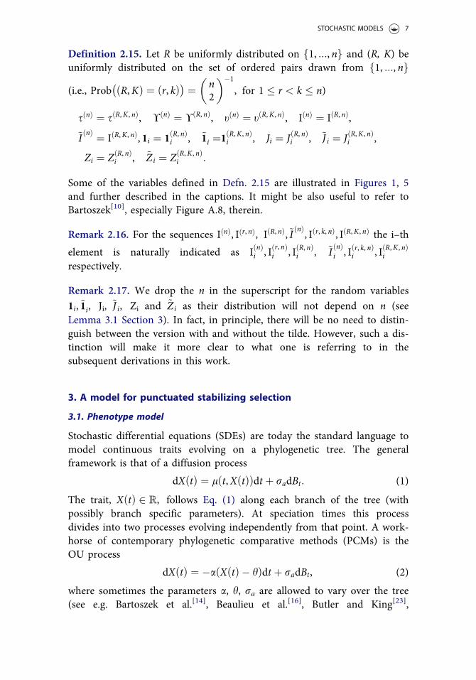
The jumps take place after the speciation event so any jump associatedwith the speciation event that split the two lineages, e.g., in Figure 1 speci-ation event 2 for the pair of lineages A and B, cannot be common to the
the two lineages. Hence, in the caption Figure 1, we have t nð ÞAB ¼ 1, see also
Remark 2.10.Furthermore, let I nð Þ be the sequence of nodes on a randomly chosen lin-
eage and J nð Þ be a binary sequence indicating if a jump took place aftereach respective node in the I nð Þ sequence. Finally, let Tk be the timebetween speciation events k and kþ 1, pk and r2c, k be respectively the prob-ability and variance of the jump just after the k–th speciation event oneach daughter lineage. It is worth recalling that both daughter lineages mayjump independently of each other. It is also worth reminding the readerthat previously (Bartoszek[10]) the jumps were homogeneous over the tree,in this manuscript we allow their properties to vary with the nodes ofthe tree.
Figure 1. A pure–birth tree with the various time components marked on it. If we “randomlysample” node “A”, then !ðnÞ ¼ 3 and the indexes of the speciation events on this random lin-
eage are IðnÞ3 ¼ 4, IðnÞ2 ¼ 2 and IðnÞ1 ¼ 1: Notice that IðnÞ1 ¼ 1 always. The between speciationtimes on this lineage are T1, T2, T3 þ T4 and T5. If we “randomly sample” the pair of extant spe-cies “A” and “B”, then tðnÞ ¼ 1 and the two nodes coalesced at time sðnÞ ¼ T3 þ T4 þ T5: Therandom index of their joint speciation event is ~I1 ¼ 1: See also Figure 5 and Bartoszek’s[10]
Figure A.8. for a more detailed discussion on relevant notation. The internal node labellings0–4 are marked on the tree. The OUj process evolves along the branches of the tree and weonly observe the trait values at the n tips. For given tip, say “A” the value of the trait process
will be denoted XðnÞA : Of course here n¼ 5.
STOCHASTIC MODELS 9
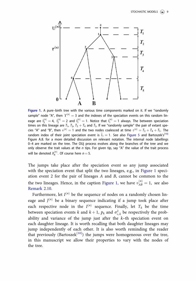
The following simple, yet very powerful, lemma comes from the uni-formity of the choice of pair to coalesce at the i–th speciation event in thebackward description of the Yule process. The proof can be found inBartoszek[10] on p. 45 (by no means do I claim this well known result asmy own).
Lemma 3.1. Consider for a Yule tree the indicator random variables 1i thatthe i–th (counting from the root) speciation event lies on a randomly selectedlineage and ~1i that the i–th speciation event lies on the path from the originto the most recent common ancestor of a randomly selected pair of tips.Then for all i 2 1, :::, n� 1f g
E ~1i �
¼ E 1i½ � ¼ Prob 1i ¼ 1ð Þ ¼ 2iþ 1
:
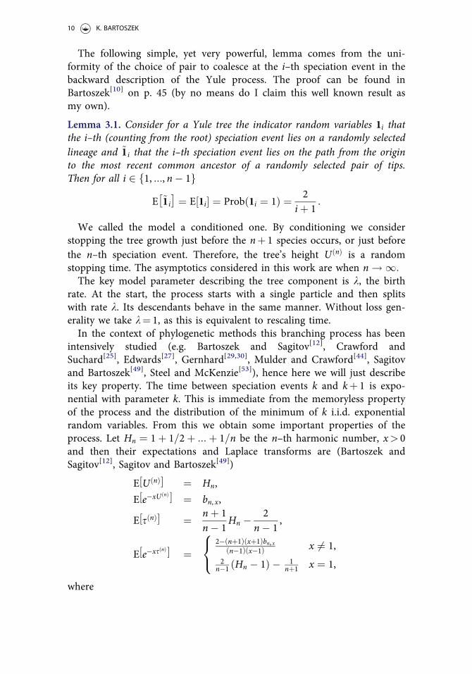
We called the model a conditioned one. By conditioning we considerstopping the tree growth just before the nþ 1 species occurs, or just beforethe n–th speciation event. Therefore, the tree’s height U nð Þ is a randomstopping time. The asymptotics considered in this work are when n ! 1:The key model parameter describing the tree component is k, the birth
rate. At the start, the process starts with a single particle and then splitswith rate k. Its descendants behave in the same manner. Without loss gen-erality we take k¼ 1, as this is equivalent to rescaling time.In the context of phylogenetic methods this branching process has been
intensively studied (e.g. Bartoszek and Sagitov[12], Crawford andSuchard[25], Edwards[27], Gernhard[29,30], Mulder and Crawford[44], Sagitovand Bartoszek[49], Steel and McKenzie[53]), hence here we will just describeits key property. The time between speciation events k and kþ 1 is expo-nential with parameter k. This is immediate from the memoryless propertyof the process and the distribution of the minimum of k i.i.d. exponentialrandom variables. From this we obtain some important properties of theprocess. Let Hn ¼ 1þ 1=2þ :::þ 1=n be the n–th harmonic number, x> 0and then their expectations and Laplace transforms are (Bartoszek andSagitov[12], Sagitov and Bartoszek[49])
E U nð Þ½ � ¼ Hn,
E e�xU nð Þ½ � ¼ bn, x,
E s nð Þ½ � ¼ nþ 1n� 1
Hn � 2n� 1
,
E e�xs nð Þ½ � ¼2� nþ1ð Þ xþ1ð Þbn, x
n�1ð Þ x�1ð Þ x 6¼ 1,2
n�1 Hn � 1ð Þ � 1nþ1 x ¼ 1,
8<:
where
10 K. BARTOSZEK
bn, x ¼ 1xþ 1
� � � nnþ x
¼ C nþ 1ð ÞC xþ 1ð ÞC nþ xþ 1ð Þ � C xþ 1ð Þn�x,
C �ð Þ being the gamma function.Now let Yn be the r–algebra that contains information on the Yule tree
and jump pattern. By this we mean that conditional on Yn we know exactlyhow the tree looks like (esp. the interspeciation times Ti) and we know atwhat parts of the tree (at which lineage(s) just after which speciation events)did jumps take place. The motivation behind such conditioning is that condi-tional on Yn the contemporary tips sample is a multivariate normal one.When one does not condition on Yn the normality does not hold—the ran-domness in the tree and presence/absence of jumps distorts normality.Bartoszek[10] previously studied the branching Ornstein–Uhlenbeck with
jumps (OUj) model and it was shown (but, therein for constant pk and r2c, kand therefore there was no need to condition on the jump pattern) that,conditional on the tree height and number of tip species the mean andvariance of the trait value of tip species r (out of the n contemporary),
X nð Þr � X nð Þ
r U nð Þð Þ (see also Figure 1), are
E X nð Þr jYn
h i¼ hþ e�aU nð Þ
X0 � hð Þ
Var X nð Þr jYn
h i¼ r2a
2a1� e�2aU nð Þ� �
þX! r, nð Þ
i¼1
r2c, I
r, nð Þi
Jr, nð Þi e
�2a Tnþ:::þTIr, nð Þi
þ1
� �,
(4)
! r, nð Þ, I r, nð Þ and J r, nð Þ are realizations of the random variables ! nð Þ, I nð Þ andJ nð Þ when lineage r is picked. A key difference that the phylogeny brings in,is that the tip measurements are correlated through the tree structure. Onecan easily show that conditional on Yn, the covariance between traits
belonging to tip species r and k, X nð Þr and X nð Þ
k is
Cov X nð Þr ,X nð Þ
k jYn
h i¼ r2a
2ae�2as r, k, nð Þ � e�2aU nð Þ� �
þXt r, k, nð Þ
i¼1
r2c, I r, k, nð Þ
i
J r, k, nð Þi e
�2a s r, k, nð Þþ:::þTIr, k, nð Þi
þ1
� �, (5)
where J r, k, nð Þ, I r, k, nð Þ correspond to the realization of random variablesJ nð Þ, I nð Þ, but reduced to the common part of lineages r and k, while
t r, k, nð Þ, s r, k, nð Þ correspond to realizations of t nð Þ, s nð Þ when the pair (r, k) ispicked. We will call, the considered model the Yule–Ornstein–Uhlenbeckwith jumps (YOUj) process.
STOCHASTIC MODELS 11
Remark 3.2. Keeping the parameter h constant on the tree is not as simpli-fying as it might seem. Varying h models have been considered since theintroduction of the OU process to phylogenetic methods (Hansen[34]).However, it can very often happen that the h parameter is constant overwhole clades, as these species share a common optimum due to some com-mon discrete characteristic. Therefore, understanding the model’s behaviorwith a constant h is a crucial first step. Furthermore, if constant h cladesare apart far enough one could think of them as independent samples andattempt to construct a test (based on normality of the species’ averages) ifjumps have a significant effect (compare Thms. 4.1 and 4.6). For this onewould have to make the very difficult to biologically justify assumption ofconstant model parameters between clades. Though, one can imagine spe-cial situations where the levels of h are connected to a discrete characteris-tic common to many clades, e.g., fresh water or seawater. On the otherhand CLTs and other asymptotical results for changing model parametersand different levels of h are an exciting future research direction.
Remark 3.3. It should be noted that the phylogeny could be introducedusing a formal branching process approach and the offspring’s’ generatingfunction (e.g. Ch. III.3, Athreya and Ney[5]). Then, the branching traitmodel can be described (jointly with the tree) as a “Markov process in thespace of integer–valued measures on R” (Adamczak and Miło�s[3]).However, in this work here we do not use any of the machinery from thatdirection and so we refrain from defining the setup in that language so asto avoid adding yet another layer of notation. On the other hand, the wayof defining the model used here is constructive—in the sense that it can bedirectly coded in a simulation procedure.
3.3. Martingale formulation
Our main aim is to study the asymptotic behavior of the sample averageand it actually turns out to be easier to work with scaled trait values, for each
r 2 1, :::, nf g, Y nð Þr ¼ X nð Þ
r � h� �
=ffiffiffiffiffiffiffiffiffiffiffiffir2a=2a
p: Denoting d ¼ X0 � hð Þ= ffiffiffiffiffiffiffiffiffiffiffiffi
r2a=2ap
we have
E Y nð Þ½ � ¼ dbn, a: (6)
The initial condition of course will be Y0 ¼ d:
Remark 3.4. We remark, that here it becomes evident that the specificvalue of h, will not play any role in obtaining the presented here results.What only matters is the initial displacement from h, but even this will not
12 K. BARTOSZEK
contribute in any way to the rate of convergence, only as a scaling constantfor the expectation of �Yn (see Proof of Thm. 4.1).Just as was done by Bartoszek and Sagitov[12] we may construct a mar-
tingale related to the average
�Yn ¼ 1n
Xni¼1
Y nð Þi :
It is worth pointing out that �Yn is observed just before the n–th speciationevent. An alternative formulation would be to observe it just after then� 1ð Þ–st speciation event. Then (cf. Lemma 10 of Bartoszek andSagitov[12], we define
Hn :¼ nþ 1ð Þe a�1ð ÞU nð Þ �Yn, n � 0:
This is a martingale with respect to Fn, the r–algebra containing informationon the Yule n–tree and the phenotype’s evolution, i.e., Fn ¼ r Yn,Y1, :::,Ynð Þ:
4. Asymptotic regimes — main results
Branching Ornstein–Uhlenbeck models commonly have three asymptoticregimes (Adamczak and Miło�s[2,3], An�e et al.[4], Bartoszek[10], Bartoszek andSagitov[12], Ren et al.[46,47]). The dependency between the adaptation rate aand branching rate k¼ 1 governs in which regime the process is. If a > 1=2,then the contemporary sample is similar to an i.i.d. sample, in the criticalcase, a ¼ 1=2, we can, after appropriate rescaling, still recover the “near” i.i.d.behavior and if 0 < a < 1=2, then the process has “long memory” (“localcorrelations dominate over the OU’s ergodic properties”, Adamczak andMiło�s[2,3]). In the context considered here by “near” and “similar” to i.i.d. wemean that the resulting CLTs resemble those of an i.i.d. sample. For examplethe limit distribution of the normalized sample average in the a > 0:5 YOUregime [Thm. 1 in 12] is N 0, 2aþ 1ð Þ= 2a� 1ð Þ� �
and taking a ! 1 weobtain the classical N 0, 1ð Þ limit (as intuition could suggest with instantan-eous adaptation). In the YOUj setup the same three asymptotic regimes canbe observed, even though Adamczak and Miło�s[2,3], Ren et al.[46,47] assumethat the tree is observed at a given time point, t, with nt being random. Inwhat follows here, the constant C may change between (in)equalities. It mayin particular depend on a. We illustrate the below Theorems in Figure 2.We consider the process �Yn ¼ �Xn � hð Þ= ffiffiffiffiffiffiffiffiffiffiffiffi
r2a=2ap
which is the normal-ized sample mean of the YOUj process with �Y 0 ¼ d: The next twoTheorems consider its, depending on a, asymptotic with n behavior.
Theorem 4.1. Assume that the jump probabilities and jump variances areconstant equaling p and r2c < 1 respectively.
STOCHASTIC MODELS 13
(I) If 0:5 < a and 0 < p < 1, then the conditional variance of the scaledsample mean r2n :¼ nVar �YnjYn
�converges in P to a finite mean and
variance random variable r21. The scaled sample mean,ffiffiffin
p�Yn converges
weakly to random variable whose characteristic function can be expressedin terms of the Laplace transform of r21
8x2R limn!1/ ffiffi
np
�Ynxð Þ ¼ L r21
� �x2=2� �
:
(II) If 0:5 ¼ a, thenffiffiffiffiffiffiffiffiffiffiffiffiffiffiffiffiffin= ln nð Þp
�Yn is asymptotically normally distributedwith mean 0 and variance 2þ 4pr2c=r
2a. In particular the conditional
variance of the scaled sample mean r2n :¼ n ln �1nVar �YnjYn
�converges
in L2 (and hence in P) to the constant 2þ 4pr2c=r2a:
(III) If 0 < a < 0:5, then na�Yn converges almost surely and in L2 to a randomvariable Ya, d with finite first two moments.
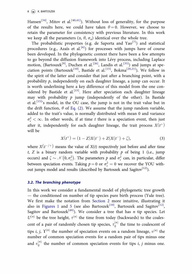
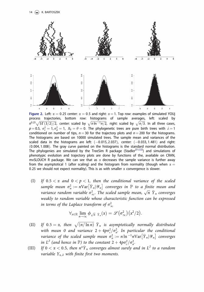
Figure 2. Left: a ¼ 0:25 center: a ¼ 0:5 and right: a¼ 1. Top row: examples of simulated YOUjprocess trajectories, bottom row: histograms of sample averages, left: scaled byn0:25
ffiffiffiffiffiffiffiffiffiffiffiffiffiffiffiffiffiffiffiffiffi5Cð3=2Þ=2p
, center: scaled byffiffiffiffiffiffiffiffiffiffiffiffiffiffiffiffiffiffiffin ln�1n=2
p, right: scaled by
ffiffiffiffiffiffiffiffin=3
p: In all three cases,
p¼ 0.5, r2c ¼ 1,r2a ¼ 1, X0 ¼ h ¼ 0: The phylogenetic trees are pure birth trees with k¼ 1conditioned on number of tips, n¼ 30 for the trajectory plots and n¼ 200 for the histograms.The histograms are based on 10000 simulated trees. The sample mean and variances of thescaled data in the histograms are left: ð�0:015, 2:037Þ, center: ð�0:033, 1:481Þ and right:ð0:004, 1:008Þ: The gray curve painted on the histograms is the standard normal distribution.The phylogenies are simulated by the TreeSim R package (Stadler[51,52]) and simulations ofphenotypic evolution and trajectory plots are done by functions of the, available on CRAN,mvSLOUCH R package. We can see that as a decreases the sample variance is further awayfrom the asymptotical 1 (after scaling) and the histogram from normality (though when a ¼0:25 we should not expect normality). This is as with smaller a convergence is slower.
14 K. BARTOSZEK
Remark 4.2. For the a.s. and L2 convergence to hold in Part 3, it sufficesthat the sequence of jump variances is bounded. Of course, the first twomoments will differ if the jump variance is not constant.
Remark 4.3. After this remark we will define the concept of a sequenceconverging to 0 with density 1. Should the reader find it easier, they mayforget that the sequence converges with density 1, but think of thesequence simply converging to 0. The condition of convergence with dens-ity 1 is a technicality that through ergodic theory allows us to slightlyweaken the assumptions of the theorem that gives a normal limit.
Definition 4.4. A subset E N of positive integers is said to have density0 (e.g., Petersen[45]) if
limn!1
1n
Xn�1
k¼0
vE kð Þ ¼ 0,
where vE �ð Þ is the indicator function of the set E.
Definition 4.5. A sequence an converges to 0 with density 1 if there existsa subset E N of density 0 such that
limn!1, n 62E
an ¼ 0:
Theorem 4.6. Assume that the sequence r4c, kpk� �
is bounded. Then, depend-ing on a the process �Yn has the following asymptotic with n behavior.
(I) If 0:5 < a, r4c, kpk 1� pkð Þ goes to 0 with density 1 and the sequencesr2c, k� �
, pkf g are such that the sequences of expectations
EX! nð Þ
k¼1
r2c, I nð Þ
k
Jke�2a Tnþ:::þT
Inð Þk
þ1
� �24
35! r2!
nEXt nð Þ
k¼1
r2c,~I
nð Þk
~Jke�2a s nð Þþ:::þT
~Inð Þk
þ1
� �24
35! r2t
converge, then the processffiffiffin
p�Yn is asymptotically normally distributed
with mean 0 and variance 2aþ 1ð Þ= 2a� 1ð Þ þ r2! þ r2t� �
= r2a= 2að Þ� �:
(II) If 0:5 ¼ a, and the sequences r2c, k� �
, pkf g are such that the sequence ofexpectations
n ln �1nð ÞEXt nð Þ
k¼1
r2c,~I
nð Þk
~Jke� s nð Þþ:::þT
~Inð Þk
þ1
� �24
35! r2t
STOCHASTIC MODELS 15
converges, thenffiffiffiffiffiffiffiffiffiffiffiffiffiffiffiffiffin= ln nð Þp
�Yn is asymptotically normally distributed withmean 0 and variance 2þ r2t=r
2a:
It is worth pointing out that Thm. 4.6 covers the extreme cases p¼ 0 and p¼ 1.The convergence conditions on the expectations look rather daunting, howeverthey will simplify very compactly if r2c, k and pk are constant or r4c, kpk ! 0 (withdensity 1). These we discuss after the proof of the theorem, when we also men-tion why the assumptions on these expectations are necessary.
Remark 4.7. In the original arXiv preprint of this paper it was stated thatconvergence to normality in the a � 0:5 regimes will only take place if r4c, kpkis bounded and goes to 0 with density 1. Normality in the a ¼ 0:5 and pk ¼1 regimes was noticed thanks to the collaboration with Torkel Erhardsson[11]
and then, the results and proofs in this manuscript were adjusted.
Remark 4.8. The assumption r4c, kpk 1� pkð Þ ! 0 with density 1 is an essen-tial one for the limit to be a normal distribution, when a > 0:5: This is vis-ible from the proof of Lemma 5.5. In fact, this is the key difference thatthe jumps bring in—if their magnitude or their uncertainty in occurrenceis too large, then they will disrupt the weak convergence.One possible way of achieving the above condition is to keep r2c, k constant
and allow pk ! 0, the chance of jumping becomes smaller relative to thenumber of species. Alternatively, r2c, k ! 0, which could mean that with moreand more species—smaller and smaller jumps occur at speciation. Actually,one could intuitively think of this as biologically more realistic. We are in theYule, no extinction, case so with time there will be more and more species(species here can be understood, if it helps intuition as non–mixing, for somereason, populations). If they all live in some spatially confined area, then asthe number of species grows there could be more and more competition. Ifone considers a trait that is related to what is competed for, then smaller andsmaller differences in phenotype could drive the species apart. Specializationoccurs and tinier and tinier niches are filled. This reasoning of course furtherassumes that the number of individuals grows with the number of species.Furthermore, under the considered YOUj model the long time mean, h, is thesame for all species, so even though there is an initial displacement (into adifferent niche) with time the trait will try to revert to its optimum. Hence,the above is not aiming for making any authoritative biological statements,nor provide an interpretation of the whole YOUj model. Rather, it has as itsgoal of giving some intuition on jump variance decreasing to 0 with time/number of species.
Remark 4.9. In Thm. 4.6 we do not consider the “fast branching/slowadaptation”, 0 < a < 0:5 regime. By assuming r4c, kpk ! 0 with density 1, it
16 K. BARTOSZEK
is possible to make the influence of the jumps disappear asymptotically,just like in the a � 0:5 case, see Example 6.6. However, no further insights,than those in Thm. 4.1 will be readily available, similarly as Bartoszek andSagitov[12] note for the YOU without jumps model. This is as the usedhere methods, do not seem to easily extend to the 0 < a < 0:5 situation,beyond what is presented in this manuscript.
5. A series of technical lemmata
We will now prove a series of technical lemmata describing the asymptoticsof driving components of the considered YOUj process. For two sequencesan, bn the notation an � bn will mean that an=bn ! C 6¼ 0 with n and an �1þ o 1ð Þð Þbn: Notice that always when an � bn is used a defined orundefined constant C is present within bn. The key property is that theasymptotic behavior with n does not change after the � sign. The generalapproach to proving these lemmata is related to that in the proof ofBartoszek and Sagitov’s[12] Lemma 11. What changes here is that we needto take into account the effects of the jumps [which were not considered in12]. However, we noticed that there is an error in the proof of Bartoszekand Sagitov’s[12] Lemma 11. Hence, below for the convenience of thereader, we do not only cite the lemma but also provide the whole correctedproof. In Remark 5.2, following the proof, we briefly point the problem inthe original wrong proof and explain why it does not influence the rest ofBartoszek and Sagitov’s[12] results.
Lemma 5.1. (Lemma 11 of Bartoszek and Sagitov[12])
Var E e�2as nð Þ jYn
h ih i¼
O n�4að Þ 0 < a < 0:75,
O n�3 ln nð Þ a ¼ 0:75,
O n�3ð Þ 0:75 < a:
8><>: (7)
Proof. For a given realization of the Yule n-tree we denote by s nð Þ1 and s nð Þ
2
two versions of s nð Þ that are independent conditional on Yn: In other
words s nð Þ1 and s nð Þ
2 correspond to two independent choices of pairs of tipsout of n available. Conditional on Yn all heights in the tree are known—
the randomness is only in the choice out of then2
� pairs or equivalently
sampling out of the set of n – 1 coalescent heights. We have,
E E e�2as nð Þ jYn
h i� �2 �¼ E E e�2a s nð Þ
1 þs nð Þ2ð ÞjYn
h ih i¼ E e�2a s nð Þ
1 þs nð Þ2ð Þ �
:
Let pn, k be the probability that two randomly chosen tips coalesced at thek–th speciation event. We know that (cf. Stadler[51]’s proof of her Theorem
STOCHASTIC MODELS 17
4.1, using m for our n or Bartoszek and Sagitov’s[12] Lemma 1 for a moregeneral statement)
pn, k ¼ 2nþ 1n� 1
1kþ 1ð Þ kþ 2ð Þ :
Writing
fa k, nð Þ :¼ kþ 1aþ kþ 1
� � � naþ n
¼ C nþ 1ð ÞC aþ kþ 1ð ÞC kþ 1ð ÞC aþ nþ 1ð Þ
and as the times between speciation events are independent and exponen-tially distributed we obtain
E E e�2as nð Þ jYn
h i� �2 �¼Xn�1
k¼1
f4a k, nð Þp2n, k
þ 2Xn�1
k1¼1
Xn�1
k2¼k1þ1
f2a k1, k2ð Þf4a k2, nð Þpn, k1pn, k2 :
On the other hand,
E e�2as nð Þ �� �2 ¼ Xn�1
k1¼1
f2a k1, nð Þpn, k1
0@
1A Xn�1
k2¼1
f2a k2, nð Þpn, k2
0@
1A:
Taking the difference between the last two expressions we find
Var E e�2as nð Þ jYn
h ih i¼Xk
f4a k, nð Þ � f2a k, nð Þ2� �
p2n, k
þ 2Xn�1
k1¼1
Xn�1
k2¼k1þ1
f2a k1, k2ð Þ f4a k2, nð Þ � f2a k2, nð Þ2� �
pn, k1pn, k2 :
Noticing that we are dealing with a telescoping sum and hence using therelation
a1 � � � an � b1 � � � bn ¼Xni¼1
b1 � � � bi�1 ai � bið Þaiþ1 � � � an (8)
we see that it suffices to study the asymptotics of,
Xn�1
k¼1
An, kp2n, k and
Xn�1
k1¼1
Xn�1
k2¼k1þ1
f2a k1, k2ð ÞAn, k2pn, k1pn, k2 ,
where
An, k :¼Xnj¼kþ1
f2a k, jð Þ2 4a2
j jþ 4að Þ
!f4a j, nð Þ:
18 K. BARTOSZEK
To consider these two asymptotic relations we observe that for large n
An, k � 4a2bn, 4ab2k, 2a
Xnj¼kþ1
b2j, 2abj, 4a
1j 4aþ jð Þ � C
bn, 4ab2k, 2a
Xnj¼kþ1
j�2 � Cbn, 4ab2k, 2a
k�1:
Now since pn, k ¼ 2 nþ1ð Þn�1ð Þ kþ2ð Þ kþ1ð Þ , it follows
Xn�1
k¼1
An, kp2n, k � Cbn, 4a
Xn�1
k¼1
1k5b2k, 2a
� Cn�4aXnk¼1
k4a�5
� C
n�4a 0 < a < 1
n�4 ln n a ¼ 1
n�4 1 < a
8><>:
and
Xn�1
k1¼1
Xn�1
k2¼k1þ1
f2a k1, k2ð ÞAn, k2pn, k1pn, k2 � Cbn, 4aXn�1
k1¼1
Xn�1
k2¼k1þ1
1bk1, 2abk2, 2a
1k21k
32
� Cn�4aXn�1
k1¼1
k2a�21
Xn�1
k2¼k1þ1
k2a�32 � C
n�4aXn�1
k1¼1
k4a�41 0 < a < 1
n�4Xnk2¼2
k�12
Xk2k1¼1
1 a ¼ 1
n�4aXnk2¼2
k4a�42 1 < a
8>>>>>>>>><>>>>>>>>>:
� C
n�4a 0 < a < 0:75n�3 ln n a ¼ 0:75n�3 0:75 < a < 1
n�4Xnk2¼2
1 a ¼ 1
n�3 1 < a
� C
n�4a 0 < a < 0:75n�3 ln n a ¼ 0:75n�3 0:75 < a < 1n�3 a ¼ 1n�3 1 < a:
8>>>><>>>>:
8>>>>>>><>>>>>>>:
Summarizing
Xn�1
k1¼1
Xn�1
k2¼k1þ1
f2a k1, k2ð ÞAn, k2pn, k1pn, k2 � Cn�4a 0 < a < 0:75n�3 ln n a ¼ 0:75n�3 0:75 < a < 1:
8<:
Remark 5.2. Bartoszek and Sagitov[12] wrongly stated in their Lemma 11
that Var E e�2as nð Þ jYn
h ih i¼ O n�3ð Þ for all a > 0: From the above we can
see that this holds only for a > 3=4: This does not however changeBartoszek and Sagitov’s[12] main results. If one inspects the proof ofTheorem 1 therein, then one can see that for a > 0:5 it is required that
STOCHASTIC MODELS 19
Var E e�2as nð Þ jYn
h ih i¼ O n� 2þ�ð Þð Þ, where � > 0: This by Lemma 5.1 holds.
Bartoszek and Sagitov’s[12] Thm. 2 does not depend on the rate of conver-
gence, only that n2Var E e�2as nð Þ jYn
h ih i! 0 with n. This remains true, just
with a different rate.
Let I nð Þ be the sequence of speciation events on a random lineage andJið Þ be the jump pattern (binary sequence 1 jump took place, 0 did nottake place just after speciation event i) on a randomly selected lineage.
Lemma 5.3. For random variables ! nð Þ, I nð Þ, Jið Þ! nð Þi¼1
� �derived from the same
random lineage and a fixed jump probability p we have
Var EX! nð Þ
i¼1
Jie�2a Tnþ:::þT
Inð Þi
þ1
� �jYn
24
35
24
35 � pC
n�4a 0 < a < 0:25n�1 ln n a ¼ 0:25n�1 0:25 < a:
8<:
(9)
Proof. We introduce the random variables
W nð Þ:¼X! nð Þ
i¼1
Jie�2a Tnþ:::þT
Inð Þi
þ1
� �
and
/i :¼ Zie
�2a Tnþ:::þTiþ1ð ÞE 1ijYn½ �,where Zi is the binary random variable if a jump took place at the i–th spe-ciation event of the tree for our considered random lineage. Obviously
E W nð Þ jYn
h i¼Xn�1
i¼1
/i :
Immediately (for i< j)
E /i
� ¼ 2piþ 1
bn, 2abi, 2a
,
E /i/
j
h i¼ 4p2
iþ 1ð Þ jþ 1ð Þbn, 4abj, 4a
bj, 2abi, 2a
,
E /i2
� ¼ pbn, 4abi, 4a
E E 1ijYn½ �ð Þ2 �
:
We illustrate the random objects defined above in Figure 5. The term
E E 1ijYn½ �ð Þ2 �
can be expressed as E 1 1ð Þi 1 2ð Þ
i
h i(same as with
E E e�2as nð Þ jYn
h i� �2 �in Lemma 5.1), where 1 1ð Þ
i and 1 2ð Þi are two copies of
20 K. BARTOSZEK
1i that are independent given Yn, i.e., for a given tree we sample two line-ages and ask if the i–th speciation event is on both of them. This will occurif these lineages coalesced at a speciation event k � i: Therefore,
E 1 1ð Þi 1 2ð Þ
i
h i¼ 2
iþ 1
Xn�1
k¼iþ1
pk, n þ pi, n ¼ nþ 1n� 1
2iþ 1
Xn�1
k¼iþ1
2kþ 1ð Þ kþ 2ð Þ þ
1iþ 2
!
¼ nþ 1n� 1
2iþ 1
2iþ 2
� 2nþ 1
þ 1iþ 2
� ¼ nþ 1
n� 16
iþ 1ð Þ iþ 2ð Þ �2
n� 12
iþ 1:
Together with the above
E /i2
� ¼ pbn, 4abi, 4a
nþ 1n� 1
6iþ 1ð Þ iþ 2ð Þ �
1n� 1
4iþ 1
� :
Now
VarXn�1
i¼1
/i
" #¼Xn�1
i¼1
E /i2
�� E /i
�� �2� �þ 2Xn�1
i¼1
Xn�1
j¼iþ1
E /i /
j
h i� E /
i
�E /
j
h i� �
¼Xn�1
i¼1
pbn, 4abi, 4a
nþ 1n� 1
6iþ 1ð Þ iþ 2ð Þ �
1n� 1
4iþ 1
� � 4p2
iþ 1ð Þ2bn, 2abi, 2a
� 2 !
þ 2Xn�1
i¼1
Xn�1
j¼iþ1
4p2
iþ 1ð Þ jþ 1ð Þbn, 4abj, 4a
bj, 2abi, 2a
� 4p2
iþ 1ð Þ jþ 1ð Þbn, 2abi, 2a
bn, 2abj, 2a
!
� 2pXn�1
i¼1
1
iþ 1ð Þ2 3bn, 4abi, 4a
� 2pbn, 2abi, 2a
� 2 !
�I
þ 4p n� 1ð Þ�1Xn�1
i¼1
bn, 4abi, 4a
3
iþ 1ð Þ2 �1
iþ 1
� �II
þ 8p2Xn�1
i¼1
Xn�1
j¼iþ1
1iþ 1ð Þ jþ 1ð Þ
bj, 2abi, 2a
bn, 4abj, 4a
� bn, 2abj, 2a
!20@
1A
0@
1A: �III
(10)
We notice that we are dealing with a telescoping sum, we take advantageof Eq. (8) again and consider the three parts in turn.�I
Xn�1
i¼1
1
iþ 1ð Þ2 3bn, 4abi, 4a
� 2pbn, 2abi, 2a
� 2 !
¼Xn�1
i¼1
1
iþ 1ð Þ2bn�1, 2a
bi, 2a
� 2 3nnþ 4a
� 2pn2
nþ 2að Þ2 !
þ3Xn�1
k¼iþ1
bk�1, 2a
bi, 2a
� 2 kkþ 4a
� k2
kþ 2að Þ2 !
bn, 4abk, 4a
!
STOCHASTIC MODELS 21
¼Xn�1
i¼1
1
iþ 1ð Þ2bn�1, 2a
bi, 2a
� 2 n2
nþ 2að Þ23� 2pð Þnþ 3� 2pð Þ4aþ n�112a2
nþ 4a
þ3Xn�1
k¼iþ1
bk�1, 2a
bi, 2a
� 2 k2
kþ 2að Þ24a2
k kþ 4að Þbn, 4abk, 4a
!
� C 3� 2pð Þn�4aXni¼1
i4a�2 þ 12a2n�4aXni¼1
i4a�3
!
� C
n�4a 0 < a < 0:25
n�1 ln n a ¼ 0:25
n�1 0:25 < a:
8><>:
�IIn�1Xn�1
i¼1
bn, 4abi, 4a
3
iþ 1ð Þ2 �1
iþ 1
� � C 3n�4a�1
Xni¼1
i4a�2 � n�4a�1Xni¼1
i4a�1
!
� �Cn�1
�IIIXn�1
i¼1
Xn�1
j¼iþ1
1iþ 1ð Þ jþ 1ð Þ
bj, 2abi, 2a
bn, 4abj, 4a
� bn, 2abj, 2a
!20@
1A
0@
1A
¼Xn�1
i¼1
Xn�1
j¼iþ1
1iþ 1ð Þ jþ 1ð Þ f2a i, jð ÞAn, j
� Cn�4aXni¼1
Xnj¼iþ1
i�1þ2aj�2þ2a � C
n�4a 0 < a < 0:25
n�1 ln n a ¼ 0:25
n�1 0:25 < a:
8><>:
(11)
Putting these together we obtain
VarXn�1
i¼1
/i
" #� pC
n�4a 0 < a < 0:25n�1 ln n a ¼ 0:25n�1 0:25 < a:
8<:
On the other hand the variance is bounded from below by III. Its asymp-totic behavior is tight as the calculations there are accurate up to a constant(independent of p). This is further illustrated by graphs in Figure 3. w
Corollary 5.4. Let pk and r2c, k be respectively the jump probability and vari-ance at the k–th speciation event, such that the sequence r4c, kpk is bounded.We have
22 K. BARTOSZEK
n ln �1nVarXn�1
i¼1
r2c, i/i
" #! 0 for a ¼ 0:25,
nVarXn�1
i¼1
r2c, i/i
" #! 0 for 0:25 < a:
iff r4c, kpk ! 0 with density 1.
Proof. We consider the case, a > 0:25: Notice that in the proof of Lemma
5.3 VarPn�1
i¼1 /i
h i� pn�4aPn�1
i¼1 i4a�2: If the jump probability and variance
are not constant, but as in the Corollary, then
VarXn�1
i¼1
r2c, i/i
" #� n�4a
Xn�1
i¼1
pir4c, ii
4a�2 þXn�1
i¼1
pir2c, ii
4a�2
!:
Notice that if pir4c, i ! 0 with density 1, then so will pir2c, i:The Corollary is a consequence of a more general ergodic property, simi-
lar to Petersen’s[45] Lemma 6.2 (p. 65). Namely take u> 0 and if a boundedsequence ai ! 0 with density 1, then
n�uXn�1
i¼1
aiiu�1 ! 0:
To show this say the sequence ai is bounded by A, let E N be the set of nat-ural numbers such that ai ! 0 if i 2 Ec and define En ¼ E [ 1, :::, nf g: Then
n�uXn�1
i¼1
aiiu�1 ¼ n�u
Xn�1
i2En�1
i¼1
aiiu�1 þ n�u
Xn�1
i 62En�1
i¼1
aiiu�1:
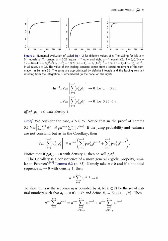
Figure 3. Numerical evaluation of scaled Eq. (10) for different values of a. The scaling for left: a ¼0:1 equals n�4a, center: a ¼ 0:25 equals n�1 log n and right a¼ 1 equals ð2pð3� 2pÞ=ð4a�1Þ � 4p=ð4aÞ þ 32p2a2ð1=ð8a2Þ þ 1=ð2að2a� 1ÞÞ � 1=ð4a2Þ�1 � 1=ðð2a� 1Þð4a� 1ÞÞÞÞn�1:In all cases, p¼ 0.5. The value of the leading constant comes from a careful treatment of the sum-mation in Lemma 5.3. The sums are approximated by definite integrals and the leading constantresulting from the integration is remembered (in the panel on the right).
STOCHASTIC MODELS 23
Denoting by jEij the cardinality of a set Ei, the former sum is bounded
above by A jEn�1jn , which, by assumption, tends to 0 as n ! 1: For the lat-
ter sum, given � > 0, if we choose N1 such that janj < �=2 for all n > N1
and N2 such that N1=nð Þu < �= 2Að Þ for all n > N2, then for all n > N ¼max N1,N2f g, one has that
n�uXn�1
i 62En�1
i¼1
aiiu�1 ¼ n�u
XN1
i 62En�1
i¼1
aiiu�1 þ n�u
Xn�1
i62En�1
i¼N1þ1
aiiu�1,
and now one has that the former sum is bounded above by An�uN1Nu�11 <
�=2 and the latter by n�unu�1 n� N1ð Þ �=2ð Þ < �=2: This proves the result.On the other hand if ai does not go to 0 with density 1,
then lim supn n�uPn�1
i¼1 aiiu�1 > 0:When a ¼ 0:25 we obtain the Corollary using the same ergodic argu-
mentation for
ln �1nXn�1
i¼1
pir4c, ii
�1 þXn�1
i¼1
pir2c, ii
�1
!:
w
Let ~Inð Þ
be the sequence of speciation events on the lineage from the originof the tree to the most recent common ancestor of a pair of randomly
selected tips and ~J i� �
be the jump pattern (binary sequence 1 jump tookplace, 0 did not take place just after speciation event i) on the lineage fromthe origin of the tree to the most recent common ancestor of a pair of ran-domly selected tips.
Lemma 5.5. For random variables t nð Þ,~Inð Þ, ~J i� �t nð Þ
i¼1
� �derived from the same
random pair of lineages and a fixed jump probability 0 < p < 1
Var EXt nð Þ
i¼1
~J ie�2a s nð Þþ:::þT
~Inð Þi
þ1
� �jYn
24
35
24
35
� p 1� pð ÞCn�4a 0 < a < 0:5,
n�2 ln n a ¼ 0:5,
n�2 0:5 < a:
8><>:
(12)
Proof. We introduce the notation
W nð Þ :¼Xt nð Þ
i¼1
~J ie�2a s nð Þþ:::þT
~Inð Þi
þ1
� �
and by definition we have
24 K. BARTOSZEK
Var EXt nð Þ
i¼1
~J ie�2a s nð Þþ:::þT
~Inð Þi
� �jYn
24
35
24
35 ¼ E E W nð ÞjYn
�� �2h i� E W nð Þ½ �ð Þ2:
We introduce the random variable
/i ¼ ~Zi~1ie�2a Tn þ :::þ Tiþ1ð Þ,
where ~Zi is the binary random variable if a jump took place just after thei–th speciation event of the tree for our considered lineage and obviously(for i1 < i2)
E /i½ � ¼ 2piþ 1
bn, 2a=bi, 2a,
E /2i
� ¼ 2piþ 1
bn, 4a=bi, 4a,
E /i1/i2
� ¼ 4p2
i1 þ 1ð Þ i2 þ 1ð Þbn, 4abi2, 4a
bi2, 2abi1, 2a
:
We illustrate the random objects defined above in Figure 5. We can write
similarly (but not exactly the same) as for W nð Þ
W nð Þ ¼Xk�1
i¼1
/i:
As usual (just as for s nð Þ1 , s nð Þ
2 in Lemma 5.1) let s nð Þ1 , t nð Þ
1 ,W nð Þ1
� �and
s nð Þ2 , t nð Þ
2 ,W nð Þ2
� �be two conditionally on Yn independent copies of
s nð Þ, t nð Þ,W nð Þ� �and now
E E W nð ÞjYn
�� �2h i¼ E E W nð Þ
1 jYn
h iE W nð Þ
2 jYn
h ih i¼ E E W nð Þ
1 W nð Þ2 jYn
h ih i¼ E W nð Þ
1 W nð Þ2
h i:
Writing out a product of two sums, for k1 < k2, as
Xk1�1
i1¼1
ai1
0@
1A Xk2�1
i2¼1
ai2
0@
1A ¼
Xk1�1
i¼1
ai
!2
þXk1�1
i1¼1
ai1
0@
1A Xk2�1
i2¼k1
ai2
0@
1A
¼Xk1�1
i¼1
a2i
!þ 2
Xk1�1
i1¼1
Xk1�1
i2¼i1þ1
ai1ai2
0@
1A
þXk1�1
i1¼1
ai1
0@
1A Xk2�1
i2¼k1
ai2
0@
1A
STOCHASTIC MODELS 25
and using the law of total probability to condition on the speciation eventat which the two nodes coalesced, we have
Var E W nð ÞjYn
� �¼ E W nð Þ
1 W nð Þ2
h i� E W nð Þ½ �ð Þ2
�I �II
¼Xn�1
k¼1
p2k, nXk�1
i¼1
E /2i
�� E /i½ �2� �
þ 2Xk�1
i1¼1
Xk�1
i2¼i1þ1
E /i1/i2
�� E /i1
�E /i2
�� �0@
1A
þ 2Xn�1
k1¼1
Xn�1
k2¼k1þ1
pk1, npk2, nXk1�1
i¼1
E /2i
�� E /i½ �2� � �III
þ2Xk1�1
i1¼1
Xk1�1
i2¼i1þ1
E /i1/i2
�� E /i1
�E /i2
�� �þXk1�1
i1¼1
Xk2�1
i2¼k1
E /i1/i2
�� E /i1
�E /i2
�� �1A:
�IV �V(13)
To aid intuition, we point out that cases I and II correspond to the casewhen the two pairs of tips coalesce at the same node k while cases III–Vwhen at different nodes, k1 < k2. We first observe
E /2i
�� E /i½ �2 ¼ 2piþ 1
bn, 4abi, 4a
� 2piþ 1
bn, 2abi, 2a
� 2 !
¼ 2piþ 1
iþ 1ð Þ2iþ 1þ 2að Þ2
iþ 1ð Þ þ 4a� 1ð Þ þ iþ 1ð Þ�14a a� 1ð Þiþ 1þ 4að Þ
bn, 4abiþ4a
þ4a2bn, 4ab2i, 2a
Xn�1
j¼iþ2
b2j, 2abj, 4a
1j jþ 4að Þ þ
bn, 2abi, 2a
� 2 n 1� 2pð Þ þ 4a 1� 2pð Þ þ n�14a2
nþ 4a
1A
and
E /i1/i2
�� E /i1
�E /i2
� ¼ 4p2
i1 þ 1ð Þ i2 þ 1ð Þbn, 4abi2, 4a
bi2, 2abi1, 2a
� bn, 2abi1, 2a
� bn, 2abi2, 2a
� �
¼ 4p2
i1 þ 1ð Þ i2 þ 1ð Þbn, 4abi2, 2abi1, 2ab
2i2, 2a
Xnj¼i2þ1
b2j, 2abj, 4a
4a2
j jþ 4að Þ
0@
1A:
(14)
Using the above, we consider each of the five components in thissum separately.
26 K. BARTOSZEK
�IXn�1
k¼1
p2k, nXk�1
i¼1
E /2i
�� E /i½ �2� �
� pCn�4aXni¼1
i4a�1 þ 4a� 1ð Þi4a�2 þ 4a a� 1ð Þi4a�3 þ 4a2i4a�2�
þ 1� 2pð Þi4a�1�Xnk¼iþ1
k�4
� pC
n�4a 0 < a < 0:75
n�3 ln n a ¼ 0:75
n�3 0:75 < a
8><>:
�IIXn�1
k¼1
p2k, nXk�1
i1¼1
Xk�1
i2¼i1þ1
E /i1/i2
�� E /i1
�E /i2
�� �
� p2Cn�4aXnk¼1
k�4Xki1¼1
i2a�11
Xki2¼i1þ1
i2a�22
� Cp2
n�4aXni1¼1
i4a�21
Xnk¼i1þ1
k�4 0 < a < 0:5
n�2Xnk¼1
k�4Xki2¼2
1 a ¼ 0:5
n�4aXni1¼1
i4a�21
Xnk¼i1þ1
k�4 0:5 < a
� Cp2n�4a 0 < a < 1
n�4 ln n a ¼ 1
n�4 1 < a
8><>:
8>>>>>>>>>><>>>>>>>>>>:
�IIIXn�1
k1¼1
Xn�1
k2¼k1þ1
pk1, npk2, nXk1�1
i¼1
E /2i
�� E /i½ �2� �
� pCn�4aXni¼1
i4a�1 þ 4a� 1ð Þi4a�2 þ 4a a� 1ð Þi4a�3 þ 4a2i4a�2�
þ 1� 2pð Þi4a�1� Xnk1¼iþ1
k�31
� p 1� pð ÞCn�4a 0 < a < 0:5
n�2 ln n a ¼ 0:5
n�2 0:5 < a
8><>:
STOCHASTIC MODELS 27
�IVXn�1
k1¼1
Xn�1
k2¼k1þ1
pk1, npk2, nXk1�1
i1¼1
Xk1�1
i2¼i1þ1
E /i1/i2
�� E /i1
�E /i2
�� �
� p2Cn�4aXnk1¼1
Xnk2¼k1þ1
k�21 k�2
2
Xk1i1¼1
Xk1i2¼i1þ1
i2a�11 i2a�2
2
� �
� p2C
n�4a 0 < a < 0:75
n�3 ln n a ¼ 0:75
n�3 0:75 < a
8><>:
�VXn�1
k1¼1
Xn�1
k2¼k1þ1
pk1, npk2, nXk1�1
i1¼1
Xk2�1
i2¼k1
E /i1/i2
�� E /i1
�E /i2
�� �
� p2Cn�4aXnk1¼1
Xnk2¼k1þ1
k�21 k�2
2
Xk1i1¼1
Xk2i2¼k1
i2a�11 i2a�2
2
� �
� p2Cn�4a
Xni1¼1
i2a�11
Xnk1¼i1þ1
k�21
Xni2¼k1
i2a�22
Xnk2¼i2þ1
k�22
!a 62 0:5, 1f g
Xnk1¼1
k�11
Xnk2¼k1þ1
k�22 Hk2
!a ¼ 0:5
12
Xn1¼k1<k2
k�12 a ¼ 1
8>>>>>>>>>>><>>>>>>>>>>>:
� p2C
n�2 a ¼ 0:5
n�4aXni1¼1
i2a�11
Xnk1¼i1þ1
k�2a�41 a 2 0, 1ð Þ n 0:5f g
n�3 a ¼ 1
n�4aXni1¼1
i2a�11
Xnk1¼i1þ1
k2a�41 1 < a
8>>>>>>>><>>>>>>>>:
� p2Cn�4a 0 < a � 0:75
n�3 ln n a ¼ 0:75
n�3 0:75 � a:
8><>:
Putting I–V together we obtain
Var E W nð ÞjYn
� �� p 1� pð ÞC
n�4a 0 < a < 0:5n�2 ln n a ¼ 0:5n�2 0:5 < a:
8<:
28 K. BARTOSZEK
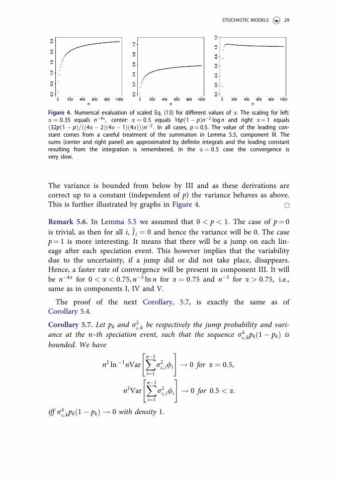
The variance is bounded from below by III and as these derivations arecorrect up to a constant (independent of p) the variance behaves as above.This is further illustrated by graphs in Figure 4. w
Remark 5.6. In Lemma 5.5 we assumed that 0 < p < 1: The case of p¼ 0is trivial, as then for all i, ~J i ¼ 0 and hence the variance will be 0. The casep¼ 1 is more interesting. It means that there will be a jump on each lin-eage after each speciation event. This however implies that the variabilitydue to the uncertainty, if a jump did or did not take place, disappears.Hence, a faster rate of convergence will be present in component III. It willbe n�4a for 0 < a < 0:75, n�3 ln n for a ¼ 0:75 and n�3 for a > 0:75, i.e.,same as in components I, IV and V.
The proof of the next Corollary, 5.7, is exactly the same as ofCorollary 5.4.
Corollary 5.7. Let pk and r2c, k be respectively the jump probability and vari-ance at the n–th speciation event, such that the sequence r4c, kpk 1� pkð Þ isbounded. We have
n2 ln �1nVarXn�1
i¼1
r2c, i/i
" #! 0 for a ¼ 0:5,
n2VarXn�1
i¼1
r2c, i/i
" #! 0 for 0:5 < a:
iff r4c, kpk 1� pkð Þ ! 0 with density 1.
Figure 4. Numerical evaluation of scaled Eq. (13) for different values of a. The scaling for left:a ¼ 0:35 equals n�4a, center: a ¼ 0:5 equals 16pð1� pÞn�2 log n and right a¼ 1 equalsð32pð1� pÞ=ðð4a� 2Þð4a� 1Þð4aÞÞÞn�2: In all cases, p¼ 0.5. The value of the leading con-stant comes from a careful treatment of the summation in Lemma 5.5, component III. Thesums (center and right panel) are approximated by definite integrals and the leading constantresulting from the integration is remembered. In the a ¼ 0:5 case the convergence isvery slow.
STOCHASTIC MODELS 29
Lemma 5.8. For random variables U nð Þ,W nð Þ and a fixed jump probability p
Cov e�2aU nð Þ, E W nð ÞjYn
�h i� pC
n�4a a < 0:5n�2 ln n a ¼ 0:5n� 2aþ1ð Þ 0:5 < a
:
8<: (15)
Proof. We introduce the random variable
�/i ¼ ~Zi~1ie�4a Tn þ :::þ Tiþ1ð Þ � 2a Ti þ :::þ T1ð Þ
and obviously
E �/i
�¼ 2p
iþ 1bn, 4a=bi, 4að Þbi, 2a:
Writing out
Cov e�2aU nð Þ, E W nð ÞjYn
�h i¼ E e�2aU nð Þ
W nð Þ �
� E e�2aU nð Þ �� �E W nð Þ½ �ð Þ
¼Xn�1
k¼1
pk, nXk�1
i¼1
E �/i
�� bn, 2aE /i½ �
� � !
¼Xn�1
k¼1
pk, nXk�1
i¼1
2piþ 1
bn, 4abi, 2abi, 4a
� b2n, 2abi, 2a
! !
¼Xn�1
k¼1
pk, nXk�1
i¼1
2piþ 1
bi, 2abn, 4abi, 4a
� bn, 2abi, 2a
� 2 !0
@1A
¼ see Eq: 11ð Þ
¼ 2pbn, 4aXn�1
k¼1
pk, nXk�1
i¼1
1iþ 1
1bi, 2a
Xnj¼iþ1
b2j, 2abj, 4a
4a2
j jþ 4að Þ
0@
1A
� Cpn�4aXni¼1
i2a�1Xn�1
k¼iþ1
k�2
� Cpn�4aXni¼1
i2a�2 � pCn�4a a < 0:5n�2 ln n a ¼ 0:5n�2a�1 0:5 < a
:
8><>:
(16)
Lemma 5.9. For random variables s nð Þ,W nð Þ and a fixed jump probability p
Cov E e�2as nð Þ jYn
h i, E W nð ÞjYn
�h i� 0 (17)
Proof. We introduce the random variable for i< k
/k, i ¼ ~Zi~1ie�4a Tn þ :::þ Tkþ1ð Þ � 2a Tk þ :::þ Tið Þ
and obviously
30 K. BARTOSZEK
/k, i ¼ 2piþ 1
bn, 4abk, 4a
bk, 2abi, 2a
:
As in the proofs of previous lemmata we denote by s nð Þ1 and W nð Þ
2 realiza-
tions of s nð Þ and W nð Þ that are conditionally independent given Yn: In other
words, given a particular Yule tree s nð Þ1 and W nð Þ
2 will correspond to twoindependent choices of pairs of tip species. In the below derivations k1 will
correspond to the node where the random pair, connected to s nð Þ1 , coa-
lesced and k2 will correspond to the node where the random pair W nð Þ2 coa-
lesced. Notice that the conditional expectation of e�2as nð Þgiven that the
coalescent took place at node k1 is bn, 2a=bk1, 2a: Writing out
Cov E e�2as nð Þ jYn
h ih i, E W nð ÞjYn
�¼ E e�2as nð Þ
1 W nð Þ2
h i� E e�2as nð Þ �� �
E W nð Þ½ �ð Þ
¼Xn�1
k¼1
p2k, nXk�1
i¼1
E /k, i
�� bn, 2abk, 2a
E /i½ �� !
�I
þXnk1¼2
Xk1�1
k2¼1
pk1, npk2, nXk2�1
i¼1
E /k1, i
�� bn, 2abk1, 2a
E /i½ �� !
�II
þXn�1
k1¼1
Xnk2¼k1þ1
pk1, npk2, nXk1i¼1
E /k1, i
�� bn, 2abk1, 2a
E /i½ �� !
�III
þXn�1
k1¼1
Xnk2¼k1þ1
pk1, npk2, nXk2�1
i¼k1þ1
E /i, k1
�� bn, 2abk1, 2a
E /i½ �� 0
@1A �IV
¼Xn�1
k¼1
p2k, nXk�1
i¼1
2piþ 1
bn, 4abk, 4a
bk, 2abi, 2a
� bn, 2abk, 2a
bn, 2abi, 2a
� !
þXnk1¼2
Xk1�1
k2¼1
pk1, npk2, nXk2�1
i¼1
2piþ 1
bn, 4abk1, 4a
bk1, 2abi, 2a
� bn, 2abk1, 2a
bn, 2abi, 2a
� !
þXn�1
k1¼1
Xnk2¼k1þ1
pk1, npk2, nXk1i¼1
2piþ 1
bn, 4abk1, 4a
bk1, 2abi, 2a
� bn, 2abk1, 2a
bn, 2abi, 2a
� !
þXn�1
k1¼1
Xnk2¼k1þ1
pk1, npk2, nXk2�1
i¼k1þ1
2piþ 1
bn, 4abi, 4a
bi, 2abk1, 2a
� bn, 2abk1, 2a
bn, 2abi, 2a
� 0@
1A:
We may recognize that, after bounding iþ 1ð Þ�1 from below by appropri-
ately k�1, k1 þ 1ð Þ�1 or k�12 , under the sums over i we will have a
STOCHASTIC MODELS 31
difference corresponding to a telescoping sum, i.e., Eq. (8). This impliesthat the whole covariance must be positive. Notice the similarity to thesums present in Eqs. (11) and (16).We also give intuition how all the individual sums arose. Component 5 cor-
responds to the case where both randomly sampled pairs coalesce at the samenode. Component 5 corresponds to the situation where the random pair oftips associated with s nð Þ coalesced later (further away from the origin of the
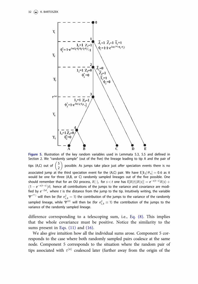
Figure 5. Illustration of the key random variables used in Lemmata 5.3, 5.5 and defined inSection 2. We “randomly sample” (out of the five) the lineage leading to tip A and the pair of
tips (A,C) out of52
� possible. As jumps take place just after speciation events there is no
associated jump at the third speciation event for the (A,C) pair. We have E½13jYn� ¼ 0:6 as itwould be one for three (A,B, or C) randomly sampled lineages out of the five possible. Oneshould remember that for an OU process, Xð�Þ, for s< t one has E½XðtÞjXðsÞ� ¼ e�aðt�sÞXðsÞ þð1� e�aðt�sÞÞh, hence all contributions of the jumps to the variance and covariance are modi-fied by e�2at , where t is the distance from the jump to the tip. Intuitively writing, the variable
WðnÞÞ will then be (for r2c, k ¼ 1) the contribution of the jumps to the variance of the randomly
sampled lineage, while WðnÞ will then be (for r2c, k � 1) the contribution of the jumps to thevariance of the randomly sampled lineage.
32 K. BARTOSZEK
tree), than the random pair associated with t nð Þ: Components 5 and 5 corres-pond to the opposite situation. In particular component 5 is when the “i”node on the path from the origin to node “t nð Þ“is earlier than or at the samenode as the coalescent associated with s nð Þ and component 5 when later. w
Remark 5.10. Notice that the proof of Lemma 5.9 can easily be continued,in the same fashion as the proofs of Lemmata 5.1–5.8 to find the rate of
the decay to 0 of Cov E e�2as nð Þ jYn
h i, E W nð ÞjYn
�h i: However, in order not
to further lengthen the technicalities we remain at showing the sign of thecovariance, as we require only this property.
6. Proof of the Central Limit Theorems 4.1 and 4.6
To avoid unnecessary notation it will be always assumed that under a given
summation sign the random variables ! nð Þ, I nð Þ, Jið Þ! nð Þi¼1
� �are derived from
the same random lineage and also t nð Þ,~Inð Þ, ~J i� �t nð Þ
i¼1
� �are derived from the
same random pair of lineages
Lemma 6.1. Conditional on Yn the first two moments of the scaled sampleaverage are
E �YnjYn
� ¼ de�aU nð Þ
E �Y 2njYn
h i¼ n�1 � 1� d2ð Þe�2aU nð Þ þ 1� n�1ð ÞE e�2as nð Þ jYn
h i
þ n�1 r2a= 2að Þ� ��1EX! nð Þ
k¼1
r2c, I nð Þ
k
Jke�2a Tnþ:::þT
Inð Þk
þ1
� ������Yn
24
35
þ 1� n�1ð Þ r2a= 2að Þ� ��1EXt nð Þ
k¼1
r2c,~I
nð Þk
~Jke�2a s nð Þþ:::þT~Ikþ1
� �����Yn
24
35,
Var �YnjYn
� ¼ n�1 � e�2aU nð Þ þ 1� n�1ð ÞE e�2as nð Þ jYn
h i
þ n�1 r2a= 2að Þ� ��1EX! nð Þ
k¼1
r2c, I nð Þ
k
Jke�2a Tnþ:::þTIkþ1ð Þ
����Yn
24
35
þ 1� n�1ð Þ r2a= 2að Þ� ��1EXt nð Þ
k¼1
r2c,~I
nð Þk
~Jke�2a s nð Þþ:::þT
~Inð Þk
þ1
� ������Yn
24
35:
STOCHASTIC MODELS 33
Proof. The first equality is immediate. The variance follows from
Var Y1 þ :::þ YnjYn½ �
¼ n 1� e�2aU nð Þ� �þ r2a= 2að Þ� ��1Xn
i¼1
X! i, nð Þ
k¼1
r2c, I i, nð Þ
k
J i, nð Þk e
�2a Tnþ:::þTIi, nð Þk
� �
þ 2Xni¼1
Xnj¼iþ1
e�2as i, j, nð Þ � e�2aU nð Þ� �
þ r2a= 2að Þ� ��1Xt i, j, nð Þ
k¼1
r2c, I
i, j, nð Þk
Ji, j, nð Þk e
�2a s i, j, nð Þþ:::þTIi, j, nð Þk
� �!
¼ n� n2e�2aU nð Þ þ n n� 1ð ÞE e�2as nð Þ jYn
h i
þ n r2a= 2að Þ� ��1EX! nð Þ
k¼1
r2c, I nð Þ
k
Jke�2a Tnþ:::þT
Inð Þk
þ1
� ������Yn
24
35
þ n n� 1ð Þ r2a= 2að Þ� ��1EXt nð Þ
k¼1
r2c,~I
nð Þk
~Jke�2a s nð Þþ:::þT
Inð Þk
� ������Yn
24
35:
This immediately entails the second moment. w
Before stating the next lemma we remind the reader of a key, for thismanuscript, result presented in Bartoszek’s[10] Appendix A.2 (top of secondcolumn, p. 55) in the case of p constant
E W nð Þ½ � ¼ p1a
2� 2aþ1ð Þ 2an�2aþ2ð Þbn, 2an�1ð Þ 2a�1ð Þ
� �a 6¼ 0:5
4n�1 Hn � 5n�1
2 nþ1ð Þ� �
a ¼ 0:5:
8><>: (18)
Lemma 6.2. Assume that the jump probability is constant, equaling0 < p < 1, at every speciation event. Let
an að Þ ¼n2a 0 < a < 0:5,n ln �1n 0:5 ¼ a,n 0:5 < a
8<:
and then for all a > 0 and n greater than some n að ÞWn :¼ an að ÞE W nð ÞjYn
�,
converges a.s. and in L1 to a random variable W1 with expectation
E W1½ � ¼2p 2aþ1ð ÞC 2aþ1ð Þ
1�2að Þ 0 < a < 0:5,
4p 0:5 ¼ a,
2p= a 2a� 1ð Þð Þ 0:5 < a:
8>><>>:
34 K. BARTOSZEK
In particular for a ¼ 0:5 (and also p¼ 1, see Remark 6.3) W1 is a constantand the convergence is a.s. and L2.
Proof. for a > 0:5 We know that E Wn½ � < CE for some constant CE, asE Wn½ � ! 2p= a 2a� 1ð Þð Þ by Eq. (20). Furthermore, by Lemma 5.5Var Wn½ � < CV , for some constant CV. Looking in detail, one can see fromEq. (20), that E Wn½ � will (from n large enough) converge monotonically toits limit. It will be decreasing with n for a > 1 and increasing for 0:5 <
a � 1: If one considers the asymptotic behavior, then the leading term willbe 4p= a 2a� 1ð Þð Þ 1þ 1= n� 1ð Þ� �
1� aC 2aþ 2ð Þn�2aþ1� �
: Direct calcula-tions show that for a > 1 it will be decreasing, as it behaves as4p= a 2a� 1ð Þð Þ 1þ 1= n� 1ð Þ� �
, for a¼ 1 it will be increasing as it behaves
as 4p 1� 5n�1ð Þ, while for for 0:5 < a < 1 it will be increasing as itbehaves as 4p= a 2a� 1ð Þð Þ 1� aC 2aþ 2ð Þn�2aþ1
� �:
Therefore, if one studies the proof of the downcrossing inequality andsubmartingale convergence theorem (e.g. Thm. 1.71, Cor. 1.72, p. 44,Medvegyev[39]) one will notice that only the monotonicity (which in theclassical submartingale convergence theorem is a consequence of thesequence being a submartingale) and boundedness of the expectations ofthe sequence of positive random variables are required for the almost sureconvergence. All of the above is met in our case for Wn.Hence, by the above Wn ! W1 a.s. for some random variable W1 and
as all expectations are finite, and the variance is uniformly bounded wehave E W1½ � < 1: This entails E Wn½ � ! E W1½ � ¼ 2p= a 2a� 1ð Þð Þ: Also wehave uniform integrability of Wnf g and hence L1 convergence.Proof for a ¼ 0:5 By Lemma 5.5 we know that Var E WnjYn½ �½ � behaves
as n�2 ln n: Therefore, Var Wn½ � ¼ a2n 0:5ð Þ � Var E WnjYn½ �r½ � � C n2 ln �2nð Þn�2 ln nð Þ ¼ C ln �1n ! 0: Therefore, Wn converges a.s. and in L2 to aconstant W1 ¼ 4p:Proof for 0 < a < 0:5 is the same as the proof for a > 0:5, except that
now the leading terms in the asymptotic behavior of E Wn½ � will bep 2aC 2aþ 2ð Þ þ 2n2a�1� �
= a 1� 2að Þð Þ: This causes the sequence ofexpectations to be increasing (from n large enough) and we may arguesimilar as when a > 0:5: From Eq. (20) we obtain E Wn½ � !2p 2aþ 1ð ÞC 2aþ 1ð Þ= 1� 2að Þ and Var Wn½ � is bounded by a constant byLemma 5.5. w
Remark 6.3. If p¼ 0, we are in the trivial case of no jumps. When p¼ 1, ina > 0:5 regime we will have Wn converging a.s. and in L2 to a constant,denoted above as E W1½ �, by the same argument that takes place for a ¼0:5, i.e., as the rate of decay to 0 of Var E WnjYn½ �½ � is faster than n�2: In
STOCHASTIC MODELS 35
the a < 0:5 regime the argumentation presented above holds for p¼ 1 andno convergence to a constant can be deduced, as Lemma 5.5 does not pro-vide a different rate of decay of Var E WnjYn½ �½ �:
Remark 6.4. It is worth noticing that Wn has a very interesting recursive
structure. Denote by W nþ1ð Þij the value that W nþ1ð Þ would take if the ran-
domly chosen pair of species would be tips i and j and by W nð Þi the value
that W nð Þwould take if tip i is sampled.
Wnþ1 ¼ nþ 1ð Þ 2nþ 1ð Þn
Xni¼1
Xnþ1
j¼iþ1
W nþ1ð Þij
¼ e�2aTnþ1n� 1n
Wn þ 2n
Xni¼1
niX! i, nð Þ
k¼1
J i, nð Þk e
�2a Tnþ:::þTIi, nð Þk
þ1
� �0@
þ 2n
Xni¼1
niXnj 6¼i
Xt i, j, nð Þ
k¼1
Ji, j, nð Þk e
�2a s i, j, nð Þþ:::þTIi, j, nð Þk
þ1
� �1A
¼ e�2aTnþ1n� 1n
Wn þ 2n
Xni¼1
niW nð Þi þ 2
n
Xni¼1
niXnj 6¼i
W nð Þij
!,
where ni is a binary random variable indicating whether it is the i–th lin-eage that split (see Figure 6). It is worth emphasizing that the sum definingWnþ1 splits according to whether one picks both members of the pair ofspecies splitting in the last speciation event or only one of them.Obviously the distribution of the vector n1, :::, nnð Þ is uniform on the
n–element set 1, 0, :::, 0ð Þ, :::, 0, :::, 0, 1ð Þ� �: In particular note
E Wnþ1jYn½ � ¼ nþ 1nþ 1þ 2a
n� 1n
Wn þ 2n2
EXni¼1
W nð Þi jYn
" #þ 2n2
EXni¼1
Xnj6¼i
W nð Þij jYn
" #0@
1A
¼ nþ 1nþ 1þ 2a
n� 1n
Wn þ 2nE W nð Þ jYn
h iþ 2n n� 1ð Þ
n2E W nð ÞjYn
��
¼ nþ 1nþ 1þ 2a
n� 1n
Wn þ 2nE W nð Þ jYn
h iþ 2 n� 1ð Þ
n2Wn
�
¼ nþ 1nþ 1þ 2a
n� 1ð Þ nþ 2ð Þn2
Wn þ 2nE W nð Þ jYn
h i�
¼ n� 1ð Þ nþ 1ð Þ nþ 2ð Þn2 nþ 1þ 2að Þ Wn þ 2 nþ 1ð Þ
n nþ 1þ 2að ÞE W nð Þ jYn
h i:
36 K. BARTOSZEK
Furthermore, Wn shows resemblance to a martingale as the coefficientn�1ð Þ nþ1ð Þ nþ2ð Þn2 nþ1þ2að Þ converges to 1 monotonically, depending on a from above or
below, while 2 nþ1ð Þn nþ1þ2að ÞE W nð Þ jYn
h i!P, L
2
0:
Proof of Theorem 4.1, Part 1, a > 0:5We will show convergence in probability of the conditional mean and vari-ance
ln :¼ ffiffiffin
pE �YnjYn
� !P 0 n ! 1r2n :¼ nVar �YnjYn
� !P r21 n ! 1,
for a finite mean and variance random variable r21: Then, due to the con-ditional normality of �Yn this will give the convergence of characteristicfunctions and the desired weak convergence, i.e.,
E eixffiffin
p ��Yn½ � ¼ E eilnx�r2nx2=2½ � ! E e�r21x2=2½ �:
Using Lemma 6.1 and that the Laplace transform of the average coales-cent time [Lemma 3 in 12] is
E e�2as nð Þij
h i¼ 2� nþ 1ð Þ 2aþ 1ð Þbn, 2a
n� 1ð Þ 2a� 1ð Þ ¼ 22a� 1
n�1 þ O n�2að Þ (19)
we can calculate
E ln½ � ¼ dE e�aU nð Þ �¼ dbn, a ¼ O n�að Þ,
Var ln½ � ¼ n E l2n �� E ln½ �� �2� �
¼ d2n E e�2aU nð Þ �� E e�aU nð Þ �� �2� �
¼ d2n bn, 2a � b2n, a� �
¼ d2anbn, 2aXnj¼1
b2j, abj, 2a
1j jþ 2að Þ ¼ O n�2aþ1ð Þ:
Therefore we have ln ! 0 in L2 and hence in P:
Remembering that r2c, k was assumed constant, equaling r2c , Lemma 6.1states that
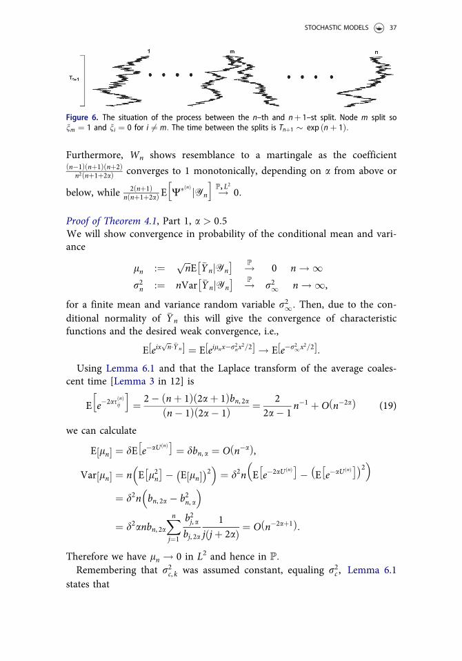
Figure 6. The situation of the process between the n–th and nþ 1–st split. Node m split sonm ¼ 1 and ni ¼ 0 for i 6¼ m: The time between the splits is Tnþ1 � exp ðnþ 1Þ:
STOCHASTIC MODELS 37
r2n ¼ 1� ne�2aU nð Þ þ n 1� n�1ð ÞE e�2as nð Þ jYn
h iþ r2a= 2að Þ� ��1
r2cE W nð Þ jYn
h iþ n 1� n�1ð Þ r2a= 2að Þ� ��1
r2cE W nð ÞjYn
�Remembering that pk was assumed constant, equaling p, we know that
1. nE e�2as nð Þ½ � ! 2= 2a� 1ð Þ (Eq. (4) in Lemma 3, Bartoszek and Sagitov[12]),
2. n2Var E e�2as nð Þ jYn
h ih i! 0 (Lemma 5.1),
3. E W nð Þ �! 2p= 2að Þ (Appendix A.2, p. 54 just above Figure A.8.,
Bartoszek[10]),
4. 4. Var E W nð Þ jYn
h ih i! 0 (Lemma 5.3),
5. 5. nE W nð ÞjYn
�!P W1 (Lemmata 5.5, 6.2).
Hence, we have nE e�2as nð Þ jYn
h i!P, L
2
2= 2a� 1ð Þ and E W nð Þ jYn
h i!P, L
2
2p= 2að Þ:Putting these individual components together we obtain
r2n!P
1þ 22a� 1
þ 2pr2cr2a
þ r2cW1r2a= 2að Þ ¼: r21:
By Lemma 6.2
E r21 � ¼ 1þ 2
2a� 1þ 2pr2c
r2aþ 4pr2c
2a� 1ð Þr2a:
Proof of Part 2, a ¼ 0:5We again show convergence in probability of the conditional mean and
variance
ln :¼ffiffiffiffiffiffiffiffiffiffiffiffiffiffiffiffiffiffiffin ln �1nð Þp
E �YnjYn
� !P 0 n ! 1r2n :¼ n ln �1nð ÞVar �YnjYn
� !P 2þ 4pr2c=r2a n ! 1:
As all the steps are the same as in Part 1 we just explicitly write the keypart concerning
r2n ¼ ln �1nð Þ 1� ne�U nð Þ� �þ n ln �1nð Þ 1� n�1ð ÞE e�s nð Þ jYn
h iþ r2c=r
2a
� �ln �1nð ÞE W nð Þ jYn
h iþ n ln �1nð Þ 1� n�1ð Þ r2c=r
2a
� �E W nð ÞjYn
�As before pk � p and we know that
1. n ln �1nð ÞE e�s nð Þ½ � ! 2 (Eq. (4) in Lemma 3, Bartoszek and Sagitov[12]),
2. n2 ln �2nð ÞVar e�s nð Þ jYn
h i! 0 (Lemma 5.1),
38 K. BARTOSZEK
3. ln �1nð ÞE W nð Þ �! 0 (Appendix A.2, p. 54 just above Figure A.8.,
Bartoszek[10]),
4. ln �2nð ÞVar E W nð Þ jYn
h ih i! 0 (Lemma 5.3),
5. n ln �1nð ÞE W nð Þ½ � ! 4p (Eq. 20), n2 ln �2nð ÞVar E W nð ÞjYn
� �! 0
(Lemma 5.5).
Putting these individual components together we obtain the L2 convergenceand hence
r2n!P
2þ 4pr2c=r2a:
Proof of Part 3, 0 < a < 0:5
We notice that the martingale (with respect to Fn) Hn ¼nþ 1ð Þe a�1ð ÞU nð Þ �Yn has uniformly bounded second moments. Namely byLemma 6.1, a modification of Lemma 5.8, Cauchy–Schwarz, bounding
E W nð Þ� �2h iby a constant and remembering that in this case r2c is constant
E H2n
� ¼ nþ 1ð Þ2E e2 a�1ð ÞU nð ÞE �Y 2
njYn
h ih i� Cn2 n�1E e�2 1�að ÞU nð Þ �
þ E e�2 1�að ÞU nð Þ�2as nð Þ ��þn�1 r2a= 2að Þ� ��1
E e�2 1�að ÞU nð ÞW nð Þ �
þ r2a= 2að Þ� ��1E e�2 1�að ÞU nð Þ
W nð Þ ��
� Cn2 n�1n�2 1�að Þ þ n�2 1�að Þn�2a þ n�1n�2 1�að Þ þ n�2� �
� C n�1þ2a þ 1þ n�1þ2a þ 1ð Þ ! C < 1:
To deal with E e�2 1�að ÞU nð ÞW nð Þ½ � one slightly modifies the proof of Lemma
5.8. Namely instead of considering the random variable �/i, consider
~Zi~1i exp � 2 Tn þ :::þ Tiþ1ð Þ þ 2 1� að Þ Ti þ :::þ T1ð Þ� �� �and then doing similar calculations one will obtain a decay of order n�2: Itis also worth pointing out that using Bartoszek and Sagitov’s[12] Lemma 3
for a more detailed consideration of E e�2 1�að ÞU nð Þ�2as nð Þ½ �, would not resultin a different rate of decay, than what Cauchy–Schwarz provides, i.e., n�2:
Hence, supn E H2n
�< 1 and by the martingale convergence theorem,
Hn ! H1 a.s. and in L2. We obtain na�Yn ! V a�1ð ÞH1 a.s. and in L2,
where V xð Þ is the a.s. and L2 limit of V xð Þn ¼ b�1
n, xe�xU nð Þ
(cf. Lemma 9 ofBartoszek and Sagitov[12]). Notice that for the convergence to hold in the0 < a < 0:5 regime, it is not required that r2c, k is constant, only bounded.
We may also obtain directly the first two moments of na�Yn (however, forthese formulae to hold, r2c, k has to be constant)
STOCHASTIC MODELS 39
naE �Yn½ � ¼ dnabn, a ! dC 1þ að Þn2aE �Y 2
n
h i¼ n2a�1 � 1� d2ð Þn2abn, 2a þ n2a 1� n�1ð ÞE e�2as nð Þ �þ n2a�1r2c r2a= 2að Þ� ��1
E W nð Þ �þ n2ar2c r2a= 2að Þ� ��1
E W nð Þ½ �
! � 1� d2ð ÞC 2aþ 1ð Þ þ 1þ 2a1� 2a
C 1þ 2að Þ 1þ 2pr2c r2a= 2að Þ� ��1� �
:
Proof of Theorem 4.6, Part 1, a > 0:5
From the proof of Part 1, Theorem 4.1 we know that ln ! 0 in probabil-ity. Then, by the assumptions of the theorem on the expectations
E r2n � ¼ n n�1 � E e�2aU nð Þ �
þ 1� n�1ð ÞE e�2as nð Þ ��
þn�1 r2a= 2að Þ� ��1EX! nð Þ
k¼1
r2c, I nð Þ
k
Jke�2a Tnþ:::þT
Inð Þk
þ1
� �24
35
þ 1� n�1ð Þ r2a= 2að Þ� ��1EXt nð Þ
k¼1
r2c,~I
nð Þk
~Jke�2a s nð Þþ:::þT
~Inð Þk
þ1
� �24
351A
! 2aþ 12a� 1
þ r2! þ r2t� �
= r2a= 2að Þ� �:
Furthermore, Lemma 5.3 (the sequence r4c, kpk is bounded by assumption)
and Corollary 5.7 (r4c, kpk 1� pkð Þ ! 0 with density 1 by assumption) imply
Var r2n � ¼ n2Var Var �YnjYn
� � ¼ n�2Var Var Y1 þ :::þ YnjYn½ �½ �� Cðn2Var e�2aU nð Þ �
þ n� 1ð Þ2Var E e�2as nð Þ jYn
h ih i
þ r2a= 2að Þ� ��2Var E
X! nð Þ
k¼1
r2c, I nð Þ
k
Jke�2a Tnþ:::þT
Inð Þk
þ1
� ������Yn
24
35
24
35
þ n� 1ð Þ2 r2a= 2að Þ� ��2Var E
Xt nð Þ
k¼1
r2c,~I
nð Þk
~Jke�2a s nð Þþ:::þT
~Inð Þk
þ1
� ������Yn
24
35
24
351A
! 0:
Therefore we obtain that r2n ! 2aþ 1ð Þ= 2a� 1ð Þ þ r2! þ r2t� �
= r2a= 2að Þ� �in probability and by convergence of characteristic functions
E eixffiffin
p ��Yn½ � ¼ E eilnx�r2nx2=2½ � ! E e� 2aþ1ð Þ= 2a�1ð Þþ r2!þr2tð Þ= r2a= 2að Þð Þ� �
x2=2h i
we obtain the asymptotic normality. Notice that on the other hand usingthe Cauchy–Schwarz inequality, Lemmata 5.8 and 5.9 we obtain
40 K. BARTOSZEK
Var r2n � � n2Var e�2aU nð Þ �
þ n� 1ð Þ2 r2a= 2að Þ� ��2Var E
Xt nð Þ
k¼1
r2c,~I
nð Þk
~Jke�2a s nð Þþ:::þT
~Inð Þk
þ1
� ������Yn
24
35
24
35þ bn að Þ,
where bn að Þ is some sequence decaying to 0 with a rate depending on a.Assume now that pk 1� pkð Þr4c, k does not converge 0 with density 1. Then,by Corollary 5.7 we will have
lim supn!1
Var EXt nð Þ
k¼1
r2c,~I
nð Þk
~Jke�2a s nð Þþ:::þT
~Inð Þk
þ1
� ������Yn
24
35
24
35 > 0
implying lim supn!1 Var r2n �
> 0 and hence, the convergence of the char-acteristic functions as above does not hold. Therefore, the convergencepk 1� pkð Þr4c, k ! 0 with density 1 is a necessary assumption for the asymp-totic normality.Proof of Part 2, a ¼ 0:5 This is proved in the same way as Part 1. Due
to the boundedness of r4c, kpk (implying r2c, kpk is bounded)
ln �1nð ÞEX! nð Þ
k¼1
r2c, I nð Þ
k
Jke� Tnþ:::þT
Inð Þk
þ1
� �24
35! 0
and as before
ln �2nð ÞVar EX! nð Þ
k¼1
r2c, I nð Þ
k
Jke� Tnþ:::þT
Inð Þk
þ1
� ������Yn
24
35
24
35! 0:
Then, due to the assumption on the expectation we have that r2n !2þ r2t=r
2a as due to the boundedness of r4c, kpk by Lemma 5.5
n2 ln �2nð ÞVar EXt nð Þ
k¼1
r2c,~I
nð Þk
~Jke� s nð Þþ:::þT
~Inð Þk
þ1
� ������Yn
24
35
24
35! 0:
Remark 6.5. The boundedness assumption for r4c, kpk (a � 0:5), togetherwith the convergence to 0 with density 1 of r4c, kpk 1� pkð Þ (for a > 0:5)
allows for controlling Var r2n �! 0: The boundedness assumption would
still allow for showing that E r2n �
is bounded but would not suffice for con-vergence. For example, consider pk � 1 constant and r2c, k ¼ 1 for k oddand 2 for k even. Then, for a > 0:5 we would have in probability
STOCHASTIC MODELS 41
lim infn!1 r2n ¼ 1þ 2
2a� 1þ 2r2a
þ 42a� 1ð Þr2a
and
lim supn!1
r2n ¼ 1þ 22a� 1
þ 4r2a
þ 8
2a� 1ð Þr2a:
It does seem that for a > 0:5 the assumption that r4c, kpk is boundedcould be relaxed. However, it would essentially require that one explicitlyassumes that the sequences r2c, k
� �, pkf g are such that the sequences of the
variances of the conditional expectations converge to 0 (as was needed forthe sequences of the expectations).
Example 6.6. Assume that r4c, kpk ! 0 with density 1. Then, by the sameergodic argument as in Corollary 5.4 and following the steps in the proofof Thm. 4.6 we obtain that for a > 0:5 we have
EX! nð Þ
k¼1
r2c, I nð Þ
k
Jke�2a Tnþ:::þT
Inð Þk
þ1
� �24
35! 0
nEXt nð Þ
k¼1
r2c,~I
nð Þk
~Jke�2a s nð Þþ:::þT
~Inð Þk
þ1
� �24
35! 0
resulting in r2n!P
2aþ 1ð Þ= 2a� 1ð Þ and for a ¼ 0:5 we have also
n ln �1nð ÞEXt nð Þ
k¼1
r2c,~I
nð Þk
~Jke� s nð Þþ:::þT
~Inð Þk
þ1
� �24
35! 0
resulting in r2n!P
2: Hence, to recover[12]’s CLTs one needs the strongerassumption of r4c, kpk ! 0 with density 1.
Acknowledgements
I would like to acknowledge Olle Nerman for his suggestion on adding jumps to thebranching OU process, Wojciech Bartoszek for helpful suggestions concerning ergodicarguments, Venelin Mitov and Tanja Stadler for many discussions. I would like to thankanonymous reviewers who found a number of errors and whose comments immenselyimproved the manuscript. I am especially grateful for pointing out a number of flaws inthe original proof of Corollary 5.4 and suggesting a significantly more elegant way of prov-ing it. I am also grateful to Torkel Erhardsson and our collaboration[11] which allowed fora correct formulation of Thms. 4.1 and 4.6.
42 K. BARTOSZEK
Funding
A significant part of this work was done at the Department of Mathematics, UppsalaUniversity, Sweden, during my postdoc which was supported by the Knut and AliceWallenberg Foundation. Currently I am supported by the Swedish Research Council(Vetenskapsrådet) grant no. 2017–04951.
ORCID
K. Bartoszek http://orcid.org/0000-0002-5816-4345
References
[1] R.; Abraham, J.-F.; Delmas, A. Continuum–Tree–Valued Markov Process. Ann.Probab. 2012, 40, 1167–1211. DOI: 10.1214/11-AOP644.
[2] Adamczak, R.; Miło�s, P. U–Statistics of Ornstein–Uhlenbeck Branching ParticleSystem. J. Theor. Probab. 2014, 27, 1071–1111. DOI: 10.1007/s10959-013-0503-2.
[3] Adamczak, R.; Miło�s, P. CLT for Ornstein–Uhlenbeck Branching Particle System.Elect. J. Probab. 2015, 20, 1–35. DOI: 10.1214/EJP.v20-4233.
[4] An�e, C.; Ho, L. S. T.; Roch, S. Phase Transition on the Convergence Rate ofParameter Estimation under an Ornstein–Uhlenbeck Diffusion on a Tree. J. Math.Biol. 2017, 74, 355–385. DOI: 10.1007/s00285-016-1029-x.
[5] Athreya, K. B.; Ney, P. E. Branching Processes. Dover Publications: New York, 2004.[6] Azaïs, R.; Dufour, F.; G�egout-Petit, A. Non–Parametric Estimation of the
Conditional Distribution of the Interjumping Times for Piecewise–DeterministicMarkov Processes. Scand. J. Statist. 2014, 41, 950–969. DOI: 10.1111/sjos.12076.
[7] de Saporta, B.; Yao, J.-F. Tail of a Linear Diffusion with Markov Switching. Ann.Appl. Probab. 2005, 15, 992–1018. DOI: 10.1214/105051604000000828.
[8] Bansaye, V.; Delmas, J.-F.; Marsalle, L.; Tran, V. C. Limit Theorems for MarkovProcesses Indexed by Continuous Time Galton–Watson Trees. Ann. Appl. Probab.2011, 21, 2263–2314. DOI: 10.1214/10-AAP757.
[9] Bartoszek, K. The Laplace Motion in Phylogenetic Comparative Methods. InProceedings of the Eighteenth National Conference on Applications of Mathematics inBiology and Medicine, Krynica Morska, 2012; pp 25–30.
[10] Bartoszek, K. Quantifying the Effects of Anagenetic and Cladogenetic Evolution.Math. Biosci 2014, 254, 42–57. DOI: 10.1016/j.mbs.2014.06.002.
[11] Bartoszek, K.; Erhardsson, T. Normal Approximation for Mixtures of NormalDistributions and the Evolution of Phenotypic Traits. ArXiv e-prints, 2019, ArXiV1912.03561. https://arxiv.org/abs/1912.03561.
[12] Bartoszek, K.; Sagitov, S. Phylogenetic Confidence Intervals for the Optimal TraitValue. J. Appl. Probab. 2015a, 52, 1115–1132. DOI: 10.1017/S0021900200113117.
[13] Bartoszek, K.; Sagitov, S. A Consistent Estimator of the Evolutionary Rate. J. Theor.Biol 2015b, 371, 69–78. DOI: 10.1016/j.jtbi.2015.01.019.
[14] Bartoszek, K.; Pienaar, J.; Mostad, P.; Andersson, S.; Hansen, T. F. A PhylogeneticComparative Method for Studying Multivariate Adaptation. J. Theor. Biol. 2012,314, 204–215. DOI: 10.1016/j.jtbi.2012.08.005.
STOCHASTIC MODELS 43
[15] Bastide, P.; Mariadassou, M.; Robin, S. Detection of Adaptive Shifts on Phylogeniesby using shifted stoch Astic Processes on a Tree. J. R. Statist. Soc. B 2017, 79,1067–1093.
[16] Beaulieu, J. M.; Jhwueng, D.-C.; Boettiger, C.; O’Meara, B. C. Modeling StabilizingSelection: Expanding the Ornstein–Uhlenbeck Model of Adaptive Evolution.Evolution 2012, 66, 2369–2389. DOI: 10.1111/j.1558-5646.2012.01619.x.
[17] Bitseki Penda, S. V.; Djellout, H.; Guillin, A. Deviation Inequalities, ModerateDeviations and Some Limit Theorems for Bifurcating Markov Chains withApplication. Ann. Appl. Probab. 2014, 24, 235–291. DOI: 10.1214/13-AAP921.
[18] Bitseki Penda, S. V.; Hoffmann, M.; Olivier, A. Adaptive Estimation for BifurcatingMarkov Chains. Bernoulli 2017, 23, 3598–3637. DOI: 10.3150/16-BEJ859.
[19] Bokma, F. Detection of Punctuated Equilibrium from Molecular Phylogenies. J.Evol. Biol. 2002, 15, 1048–1056. DOI: 10.1046/j.1420-9101.2002.00458.x.
[20] Bokma, F. Testing for Equal Rates of Cladogenesis in Diverse Taxa. Evolution 2003,57, 2469–2474. DOI: 10.1554/03-293.
[21] Bokma, F. Detection of “Punctuated Equilibrium” by Bayesian Estimation ofSpeciation and Extinction Rates, Ancestral Character States, and Rates of Anageneticand Cladogenetic Evolution on a Molecular Phylogeny. Evolution 2008, 62,2718–2726. DOI: 10.1111/j.1558-5646.2008.00492.x.
[22] Bokma, F. Time, Species and Seperating Their Effects on Trait Variance in Clades.Syst. Biol. 2010, 59, 602–607. DOI: 10.1093/sysbio/syq029.
[23] Butler, M. A.; King, A. A. Phylogenetic Comparative Analysis: A ModellingApproach for Adaptive Evolution. Am. Nat. 2004, 164, 683–695. DOI: 10.1086/426002.
[24] Cloez, B.; Hairer, M. Exponential Ergodicity for Markov Processes with RandomSwitching. Bernoulli 2015, 21, 505–1018. DOI: 10.3150/13-BEJ577.
[25] Crawford, F. W.; Suchard, M. A. Diversity, Disparity, and Evolutionary RateEstimation for Unresolved Yule Trees. Syst. Biol. 2013, 62, 439–455. DOI: 10.1093/sysbio/syt010.
[26] Duchen, P.; Leuenberger, C.; Szil�agyi, S. M.; Harmon, L.; Eastman, J.; Schweizer, M.;Wegmann, D. Inference of Evolutionary Jumps in Large Phylogenies Using L�evyProcesses. Syst. Biol. 2016, 66, 950–963. DOI: 10.1093/sysbio/syx028.
[27] Edwards, A. W. F. Estimation of the Branch Points of a Branching DiffusionProcess. J. Roy. Stat. Soc. B 1970, 32, 155–174. DOI: 10.1111/j.2517-6161.1970.tb00828.x.
[28] Eldredge, N.; Gould, S. J. Punctuated Equilibria: An Alternative to PhyleticGradualism. In Models in Paleobiology; Schopf, T. J. M., Thomas, J. M., Eds;Freeman Cooper: San Francisco, 1972; pp 82–115.
[29] Gernhard, T. The Conditioned Reconstructed Process. J. Theor. Biol. 2008, 253,769–778. DOI: 10.1016/j.jtbi.2008.04.005.
[30] Gernhard, T. New Analytic Results for Speciation Times in Neutral Models. Bull.Math. Biol. 2008, 70, 1082–1097. DOI: 10.1007/s11538-007-9291-0.
[31] Gould, S. J.; Eldredge, N. Punctuated Equilibria: The Tempo and Mode of EvolutionReconsidered. Paleobiology 1977, 3, 115–151. DOI: 10.1017/S0094837300005224.
[32] Gould, S. J.; Eldredge, N. Punctuated Equilibrium Comes of Age. Nature 1993, 366,223–227. DOI: 10.1038/366223a0.
[33] Guyon, J. Limit Theorems for Bifurcating Markov Chains. Application to theDetection of Cellular Aging. Ann. Appl. Probab. 2007, 17, 1538–1569. DOI: 10.1214/105051607000000195.
44 K. BARTOSZEK
[34] Hansen, T. F. Stabilizing Selection and the Comparative Analysis of Adaptation.Evolution 1997, 51, 1341–1351. DOI: 10.2307/2411186.
[35] Landis, M. J.; Schraiber, J. G.; Liang, M. Phylogenetic Analysis Using L�evyProcesses: finding Jumps in the Evolution of Continuous Traits. Syst. Biol. 2013, 62,193–204. DOI: 10.1093/sysbio/sys086.
[36] Marguet, A. Uniform Sampling in a Structured Branching Population. Bernoulli2019, 25, 2649–2695. DOI: 10.3150/18-BEJ1066.
[37] Mattila, T. M.; Bokma, F. Extant Mammal Body Masses Suggest PunctuatedEquilibrium. Proc. R Soc. B 2008, 275, 2195–2199. DOI: 10.1098/rspb.2008.0354.
[38] Mayr, E. Speciation and Macroevolution. Evolution 1982, 36, 1119–1132. DOI: 10.2307/2408147.
[39] Medvegyev, P. Stochastic Integration Theory. Oxford University Press: Oxford, 2007.[40] Mitov, V.; Bartoszek, K.; Stadler, T. Automatic Generation of Evolutionary
Hypotheses Using Mixed Gaussian Phylogenetic Models. Proc. Natl. Acad. Sci. USA.2019, 116, 16921–16926. DOI: 10.1073/pnas.1813823116.
[41] Mitov, V.; Bartoszek, K.; Asimomitis, G.; Stadler, T. Fast Likelihood Calculation forMultivariate Gaussian Phylogenetic Models with Shifts. Theor. Pop. Biol. 2020, 131,66–78. DOI: 10.1016/j.tpb.2019.11.005.
[42] Mooers, A. Ø.; Schluter, D. Fitting Macroevolutionary Models to Phylogenies: AnExample Using Vertebrate Body Sizes. Contrib. Zool. 1998, 68, 3–18. DOI: 10.1163/18759866-06801001.
[43] Mooers, A. Ø.; Vamosi, S. M.; Schluter, D. Using Phylogenies to TestMacroevolutionary Hypotheses of Trait Evolution in Cranes (Gruinae). Am. Nat.1999, 154, 249–259. DOI: 10.1086/303226.
[44] Mulder, W. H.; Crawford, F. W. On the Distribution of Interspecies Correlation forMarkov Models of Character Evolution on Yule Trees. J. Theor. Biol. 2015, 364,275–283. DOI: 10.1016/j.jtbi.2014.09.016.
[45] Petersen, K. Ergodic Theory. Cambridge University Press: Cambridge, 1983.[46] Ren, Y.-X.; Song, R.; Zhang, R. Central Limit Theorems for Supercritical Branching
Markov Processes. J. Func. Anal. 2014, 266, 1716–1756. DOI: 10.1016/j.jfa.2013.10.015.[47] Ren, Y.-X.; Song, R.; Zhang, R. Central Limit Theorems for Supercritical
Superprocesses. Stoch. Proc. Appl. 2015, 125, 428–457. DOI: 10.1016/j.spa.2014.09.014.[48] Ren, Y.-X.; Song, R.; Zhang, R. Central Limit Theorems for Supercritical Branching
Nonsymmetric Markov Processes. Ann. Probab. 2017, 45, 564–623. DOI: 10.1214/14-AOP987.
[49] Sagitov, S.; Bartoszek, K. Interspecies Correlation for Neutrally Evolving Traits. J.Theor. Biol. 2012, 309, 11–19. DOI: 10.1016/j.jtbi.2012.06.008.
[50] Simpson, G. G. Tempo and Mode in Evolution. Columbia University Press: NewYork, 1947.
[51] Stadler, T. On Incomplete Sampling under Birth-Death Models and Connections tothe Sampling-Based Coalescent. J. Theor. Biol 2009, 261, 58–68. DOI: 10.1016/j.jtbi.2009.07.018.
[52] Stadler, T. Simulating Trees with a Fixed Number of Extant Species. Syst. Biol 2011,60, 676–684. DOI: 10.1093/sysbio/syr029.
[53] Steel, M.; McKenzie, A. Properties of Phylogenetic Trees Generated by Yule–TypeSpeciation Models. Math. Biosci 2001, 170, 91–112. DOI: 10.1016/S0025-5564(00)00061-4.
STOCHASTIC MODELS 45