a century of numerical weather prediction: the view...
TRANSCRIPT
UL 18th March, 2005
A Century ofNumerical Weather Prediction:
The View from Limerick
Peter [email protected]
Meteorology & Climate Centre, University College Dublin
SeminarDept. of Mathematics & Statistics
University of Limerick

The Pre-history of Numerical
Weather Prediction
(circa 1900)
Vilhelm Bjerknes, Max Margules and Lewis Fry Richardson
2

Vilhelm Bjerknes (1862–1951)
Vilhelm Bjerknes on the quay at Bergen, painted by Rolf Groven, 1983
3

Vilhelm Bjerknes (1862–1951)
• Born in March, 1862.• Matriculated in 1880.• Fritjøf Nansen was a fellow-student.• Paris, 1989–90.
Studied under Poincare.• Bonn, 1890–92.
Worked with Heinrich Hertz.Vilhelm Bjerknes
• Worked in Stockholm, 1983–1907.• 1898: Circulation theorems published• 1904: Meteorological Manifesto• Christiania (Oslo), 1907–1912.• Leipzig, 1913–1917.• Bergen, 1917–1926.• 1919: Frontal Cyclone Model.
• Oslo, 1926 — 1951. Retired 1937. Died, April 9,1951.
4

Bjerknes’ 1904 ManifestoTo establish a science of meteorology, with the aim of pre-dicting future states of the atmosphere from the presentstate.“If it is true . . . that atmospheric states develop according to physi-
cal law, then . . . the conditions for the rational solution of forecasting
problems are:
5

Bjerknes’ 1904 ManifestoTo establish a science of meteorology, with the aim of pre-dicting future states of the atmosphere from the presentstate.“If it is true . . . that atmospheric states develop according to physi-
cal law, then . . . the conditions for the rational solution of forecasting
problems are:
1. An accurate knowledge of the state of the atmosphereat the initial time.
2. An accurate knowledge of the physical laws according towhich one state . . . develops from another.”
Step (1) is Diagnostic.Step (2) is Prognostic.
5

Graphical v. Numerical Approachx
Bjerknes ruled out analytical solution of the mathematicalequations, due to their nonlinearity and complexity:
“For the solution of the problem in thisform, graphical or mixed graphical andnumerical methods are appropriate, whichmethods must be derived either from thepartial differential equations or from thedynamical-physical principles which arethe basis of these equations.”
6

The First Reading from
The Book of Limerick
7

The First Reading from
The Book of Limerick
Bill Bjerknes defined, with conviction,The science of weather prediction:
7

The First Reading from
The Book of Limerick
Bill Bjerknes defined, with conviction,The science of weather prediction:
By chart diagnosis,And graphic prognosis,
7

The First Reading from
The Book of Limerick
Bill Bjerknes defined, with conviction,The science of weather prediction:
By chart diagnosis,And graphic prognosis,
The forecast is rendered non-fiction.
7

The Impossibility of ForecastingIn 1904, Max Margules contributed a short paper for theFestschrift published to mark the sixtieth birthday of hisformer teacher, the renowned physicist Ludwig Boltzmann.
Uber die Beziehung zwischen Barometerschwankungen
und Kontinuitatsgleichung. Boltzmann-Festschrift, Leipzig.
Margules considered the possibility of predicting pressurechanges by means of the continuity equation.
8

The Impossibility of ForecastingIn 1904, Max Margules contributed a short paper for theFestschrift published to mark the sixtieth birthday of hisformer teacher, the renowned physicist Ludwig Boltzmann.
Uber die Beziehung zwischen Barometerschwankungen
und Kontinuitatsgleichung. Boltzmann-Festschrift, Leipzig.
Margules considered the possibility of predicting pressurechanges by means of the continuity equation.
He showed that, to obtain an accurate estimate of the pres-sure tendency, the winds would have to be known to a pre-cision quite beyond the practical limit.
He concluded that any attempt to forecast synoptic changesby this means was doomed to failure.
A translation of Margules’ 1904 paper, together with a short introduction, has been
published as a Historical Note by Met Eireann.
8

The Vienna SchoolMany outstanding scientists were active in meteorologicalstudies in Austria in the period 1890–1925, and great progresswas made in dynamic and synoptic meteorology and in cli-matology during this time.
Julius Hann Josef Pernter
Wilhelm Trabert Felix Exner
Wilhelm Schmidt Heinrich Ficker
Albert Defant Max Margules
9

Max Margules (1856–1920)
Photograph from the archives of Zentralanstalt fur
Meteorologie und Geodynamik, Wien.
Margules was born in thetown of Brody, in westernUkraine, in 1856.
He studied mathematics andphysics at Vienna University,and among his teachers wasLudwig Boltzmann.
In 1882 he joined the Mete-orological Institute as an As-sistant, and continued to workthere for 24 years.
10

Some of Margules’ AchievementsMargules studied the diurnal and semi-diurnal variations inatmospheric pressure due to solar radiative forcing.
He derived two species of solutions of the Laplace tidalequations, which he called Wellen erster Art and Wellenzweiter Art
This was the first identification of the distinct types of wavesnow known as inertia-gravity waves and rotational waves.
? ? ?
11

Some of Margules’ AchievementsMargules studied the diurnal and semi-diurnal variations inatmospheric pressure due to solar radiative forcing.
He derived two species of solutions of the Laplace tidalequations, which he called Wellen erster Art and Wellenzweiter Art
This was the first identification of the distinct types of wavesnow known as inertia-gravity waves and rotational waves.
? ? ?
Margules showed that the available potential energy associ-ated with horizontal temperature contrasts within a midlat-itude cyclone was sufficient to explain the observed winds.
This work suggested that there were sloping frontal surfacesassociated with mid-latitude depressions, and foreshadowedthe frontal theory which emerged about a decade later.
11
A Meteorological TragedyMargules was an introverted and lonely man, who nevermarried and worked in isolation, not collaborating withother scientists.
He was disappointed and disillusioned at the lack of recog-nition of his work and retired from the Meteorological In-stitute in 1906, aged only fifty, on a modest pension.
12

A Meteorological TragedyMargules was an introverted and lonely man, who nevermarried and worked in isolation, not collaborating withother scientists.
He was disappointed and disillusioned at the lack of recog-nition of his work and retired from the Meteorological In-stitute in 1906, aged only fifty, on a modest pension.
Its value was severely eroded during the First World War sothat his 400 crowns per month was worth about one Euro,insufficient for more than the most meagre survival.
His colleagues tried their best to help him, making repeatedoffers of help which Margules resolutely resisted.
He died of starvation in 1920.
12

A Layer of Incompressible FluidThe physical principle of mass conservation is expressedmathematically in terms of the continuity equation
∂ρ
∂t+∇·ρV = 0
? ? ?
13

A Layer of Incompressible FluidThe physical principle of mass conservation is expressedmathematically in terms of the continuity equation
∂ρ
∂t+∇·ρV = 0
? ? ?
Under hydrostatic balance the pressure at a point is deter-mined by the weight of air above it.
13

A Layer of Incompressible FluidThe physical principle of mass conservation is expressedmathematically in terms of the continuity equation
∂ρ
∂t+∇·ρV = 0
? ? ?
Under hydrostatic balance the pressure at a point is deter-mined by the weight of air above it.
We can replace the atmosphere by an incompressible fluidlayer of finite depth. We take the density to be numericallyequal to one (i.e., ρ = 1kgm−3, comparable to air).
Then, if the depth is ten kilometres (or h = 104 m), thepressure is p = ρgh = 1× 10× 104 = 105 Pa = 1 atm.
In other words, this ten-kilometre layer of incompressiblefluid of unit density gives rise to a surface pressure similarto that of the compressible atmosphere.
13
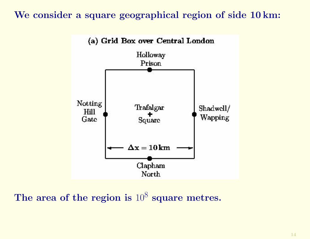
We consider a square geographical region of side 10 km:
The area of the region is 108 square metres.
14

The column of fluid above this square forms a cube whosevolume is the area multiplied by the depth:
V = 108 × 104 = 1012 m3
The total mass of fluid contained in the cube (in kg) has thesame numerical value as the volume:
M = 1012 kg = 1000 megatonnes15

Convergence and DivergenceHow does the pressure at a point change?
16
Convergence and DivergenceHow does the pressure at a point change?Since pressure is due to the weight of fluid above the pointin question, the only way it can change is through fluxesof air into or out of the column above the point.
Nett inward and outward fluxes are respectively calledconvergence and divergence.
16

Convergence and DivergenceHow does the pressure at a point change?Since pressure is due to the weight of fluid above the pointin question, the only way it can change is through fluxesof air into or out of the column above the point.
Nett inward and outward fluxes are respectively calledconvergence and divergence.
A difficulty arises because the nett convergence or diver-gence is a small difference between two large numbers.
? ? ?
Suppose that the movement of air is from west to east, sothat no air flows through the north or south faces of ourcubic column.
Assume for now that the wind speed has a uniform value often metres per second.
16

17
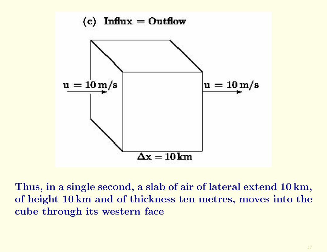
Thus, in a single second, a slab of air of lateral extend 10 km,of height 10 km and of thickness ten metres, moves into thecube through its western face
17

The slab of air moving into the cube has volume
Vin = 109 m3
Its mass has the same numerical value (since ρ = 1):
Min = 109 kg
So the mass of the cube would increase by 109 kg, or onemegatonne per second if there were only inward flux.
18

The slab of air moving into the cube has volume
Vin = 109 m3
Its mass has the same numerical value (since ρ = 1):
Min = 109 kg
So the mass of the cube would increase by 109 kg, or onemegatonne per second if there were only inward flux.
However, there is a corresponding flux of air outward throughthe eastern face of the cube, with precisely the same value.
So, the nett flux is zero:
(Flux)in = (Flux)out
The total mass of air in the cube is unchanged, and thesurface pressure remains constant.
18

Now suppose that the flow speed inward through the west-ern face of the cube is slightly greater, let us say 1% greater:
uin = 10.1 ms−1 , uout = 10.0 ms−1
19

Now suppose that the flow speed inward through the west-ern face of the cube is slightly greater, let us say 1% greater:
uin = 10.1 ms−1 , uout = 10.0 ms−1
There is thus more fluid flowing into the cube than out.There is a nett convergence of mass into the cube.
19
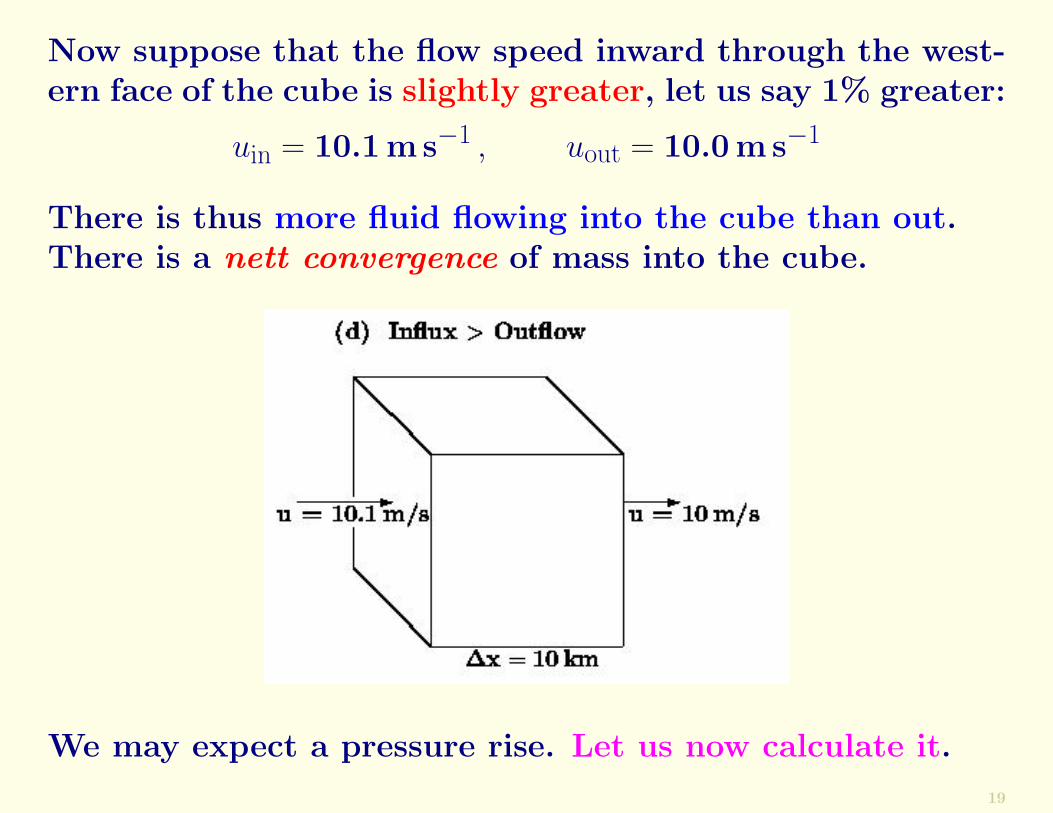
Now suppose that the flow speed inward through the west-ern face of the cube is slightly greater, let us say 1% greater:
uin = 10.1 ms−1 , uout = 10.0 ms−1
There is thus more fluid flowing into the cube than out.There is a nett convergence of mass into the cube.
We may expect a pressure rise. Let us now calculate it.
19

The additional inward flux of mass is 1% of the total inwardflux:
∆(Flux)in = 0.01× 109 = 107 kg s−1
Initially, the total mass of the cube was M = 1012 kg, so thefractional increase in mass in one second is
∆M
M=
107
1012= 10−5
20

The additional inward flux of mass is 1% of the total inwardflux:
∆(Flux)in = 0.01× 109 = 107 kg s−1
Initially, the total mass of the cube was M = 1012 kg, so thefractional increase in mass in one second is
∆M
M=
107
1012= 10−5
Pressure is proportional to mass. Therefore, the fractionalincrease in pressure is precisely the same.
To get the rate of increase in pressure, we multiply the
total pressure by this ratio:
dp
dt=
∆M
M× p = 10−5 × 105 = 1Pa s−1
The rate of pressure increase is one Pascal per second.
20

A pressure tendency of 1Pa s−1 may not sound impressivebut, if sustained over a long period of time, it is dramatic.
21
A pressure tendency of 1Pa s−1 may not sound impressivebut, if sustained over a long period of time, it is dramatic.
We recall that there are 86,400 seconds in a day. For sim-plicity, we define a “day” to be 105 s (∼28 hours).
21
A pressure tendency of 1Pa s−1 may not sound impressivebut, if sustained over a long period of time, it is dramatic.
We recall that there are 86,400 seconds in a day. For sim-plicity, we define a “day” to be 105 s (∼28 hours).
The pressure change in a “day” will then be the tendency(dp/dt) multiplied by the number of seconds in a “day”:
∆p = (1Pa s−1)× (105 s) = 105 Pa
Thus, the pressure will increase by 105 Pascals in a day.
21

A pressure tendency of 1Pa s−1 may not sound impressivebut, if sustained over a long period of time, it is dramatic.
We recall that there are 86,400 seconds in a day. For sim-plicity, we define a “day” to be 105 s (∼28 hours).
The pressure change in a “day” will then be the tendency(dp/dt) multiplied by the number of seconds in a “day”:
∆p = (1Pa s−1)× (105 s) = 105 Pa
Thus, the pressure will increase by 105 Pascals in a day.
But this is the same as its initial value, so:
The pressure increases by 100% in a day!
21

A pressure tendency of 1Pa s−1 may not sound impressivebut, if sustained over a long period of time, it is dramatic.
We recall that there are 86,400 seconds in a day. For sim-plicity, we define a “day” to be 105 s (∼28 hours).
The pressure change in a “day” will then be the tendency(dp/dt) multiplied by the number of seconds in a “day”:
∆p = (1Pa s−1)× (105 s) = 105 Pa
Thus, the pressure will increase by 105 Pascals in a day.
But this is the same as its initial value, so:
The pressure increases by 100% in a day!And this is due to a difference in wind speed so small thatwe cannot even measure it (∆u = 0.1ms−1).
21

An even more paradoxical conclusion is reached if we con-sider the speed at the western face to be 1% less than theoutflow speed at the eastern face.
The above reasoning would suggest a decrease of pressureby 100% in a day, resulting in a total vacuum and leavingthe citizens of London quite breathless.
? ? ?
22

An even more paradoxical conclusion is reached if we con-sider the speed at the western face to be 1% less than theoutflow speed at the eastern face.
The above reasoning would suggest a decrease of pressureby 100% in a day, resulting in a total vacuum and leavingthe citizens of London quite breathless.
? ? ?
Of course, there is a blunder in the reasoning: as the massin the ‘cube’ decreases, its volume must decrease in propor-tion, since the density is constant.
The fluid depth, which we took to be constant, must de-crease.
? ? ?
Margules concluded that any attempt to forecast the weatherwas “immoral and damaging to the characterof a meteorologist” (Fortak, 2001).
22

The Second Reading from
The Book of Limerick
23
The Second Reading from
The Book of Limerick
Said Margules, with trepidation,“There’s hazards with mass conservation:
23

The Second Reading from
The Book of Limerick
Said Margules, with trepidation,“There’s hazards with mass conservation:
Gross errors you’ll seeIn dee-pee-dee-tee,
23

The Second Reading from
The Book of Limerick
Said Margules, with trepidation,“There’s hazards with mass conservation:
Gross errors you’ll seeIn dee-pee-dee-tee,
Arising from blind computation”.
23

Gravity WavesWhile the calculated pressure tendency is arithmeticallycorrect, the resulting pressure change over a day is meteo-rologically preposterous. Why?
? ? ?
24

Gravity WavesWhile the calculated pressure tendency is arithmeticallycorrect, the resulting pressure change over a day is meteo-rologically preposterous. Why?
? ? ?
We have extrapolated the instantaneous pressure change,assuming it to remain constant over a long time period.
An increase of pressure within the cube causes an immediateoutward pressure gradient which opposes further change.
Indeed, the result of this negative feedback is for over-compensation, and a cycle of pressure oscillations ensues.
24

These oscillations are known as gravity waves, and they ra-diate outwards with high speed from a localised disturbance,dispersing it over a wider area.
As soon as an imbalance arises in the atmosphere, thesegravity waves act in such a way as to restore balance.
25

These oscillations are known as gravity waves, and they ra-diate outwards with high speed from a localised disturbance,dispersing it over a wider area.
As soon as an imbalance arises in the atmosphere, thesegravity waves act in such a way as to restore balance.
Since they are of high frequency, they result in pressurechanges which are large but which oscillate rapidly in time:
The instantaneous rate of change is not a re-liable indicator of the long-term change.
The computational time step has to be short enough to allowthe adjustment process to take place.
Then, gravity-wave oscillations may be present, but theyneed not spoil the forecast.
25

Gravity-wave oscillations may be effectively removed by aminor adjustment of the initial data ; this process is calledinitialization.
Modern numerical forecasts are made using the continuityequation, but initialization controls excessive gravity wavenoise and a small time step ensures that the calculationsremain stable.
? ? ?
26

Gravity-wave oscillations may be effectively removed by aminor adjustment of the initial data ; this process is calledinitialization.
Modern numerical forecasts are made using the continuityequation, but initialization controls excessive gravity wavenoise and a small time step ensures that the calculationsremain stable.
? ? ?
Bjerknes ruled out analytical solution of the mathematicalequations, due to their nonlinearity and complexity.
However, there was a scientist more bold — or foolhardy— than Bjerknes, who actually tried to calculate futureweather. This was Lewis Fry Richardson
26
Richardson’s ForecastDuring the First World War, Lewis Fry Richardson carriedout a manual calculation of the change in pressure over Cen-tral Europe (Richardson, 1922).
His initial data were based on a series of synoptic chartspublished in Leipzig by Vilhelm Bjerknes.
Using Bjerknes’ charts, he extracted the relevant values ona discrete grid, and computed the rate of change of pressurefor a region in Southern Germany.
27

Richardson’s ForecastDuring the First World War, Lewis Fry Richardson carriedout a manual calculation of the change in pressure over Cen-tral Europe (Richardson, 1922).
His initial data were based on a series of synoptic chartspublished in Leipzig by Vilhelm Bjerknes.
Using Bjerknes’ charts, he extracted the relevant values ona discrete grid, and computed the rate of change of pressurefor a region in Southern Germany.
To do this, he used the continuity equation, employing pre-cisely the method which Margules had shown more than tenyears earlier to be seriously problematical.
As is well known, the resulting “prediction” of pressurechange was completely unrealistic.
27
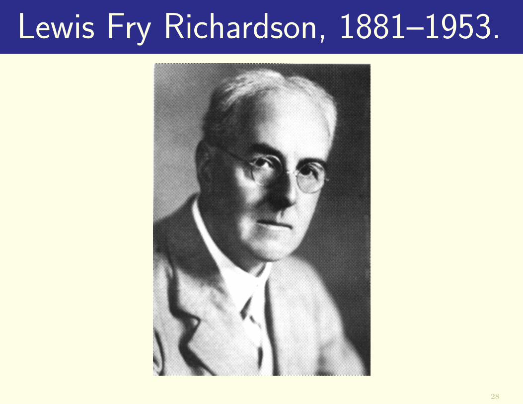
Lewis Fry Richardson, 1881–1953.
28

• Born, 11 October, 1881, Newcastle-upon-Tyne
• Family background: well-known quaker family
• 1900–1904: Kings College, Cambridge
• 1913–1916: Met. Office. Superintendent,Eskdalemuir Observatory
• Resigned from Met Office in May, 1916.Joined Friends’ Ambulance Unit.
• 1919: Re-employed by Met. Office
• 1920: M.O. linked to the Air Ministry.LFR Resigned, on grounds of concience
• 1922: Weather Prediction by Numerical Process
• 1926: Break with Meteorology.Worked on Psychometric Studies.Later on Mathematical causes of Warfare
• 1940: Resigned to pursue “peace studies”
• Died, September, 1953.
Richardson contributed to Meteorology, Numerical Analysis, Fractals,
Psychology and Conflict Resolution.29
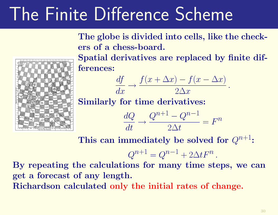
The Finite Difference SchemeThe globe is divided into cells, like the check-ers of a chess-board.Spatial derivatives are replaced by finite dif-ferences:
df
dx→ f (x + ∆x)− f (x−∆x)
2∆x.
Similarly for time derivatives:
dQ
dt→ Qn+1 −Qn−1
2∆t= Fn
This can immediately be solved for Qn+1:
Qn+1 = Qn−1 + 2∆tFn .By repeating the calculations for many time steps, we canget a forecast of any length.Richardson calculated only the initial rates of change.
30

The Leipzig Charts for 0700 UTC, May 20, 1910
Bjerknes’ sea level pressureanalysis.
Bjerknes’ 500 hPa heightanalysis.
Some of the initial data for Richardson’s “forecast”.31
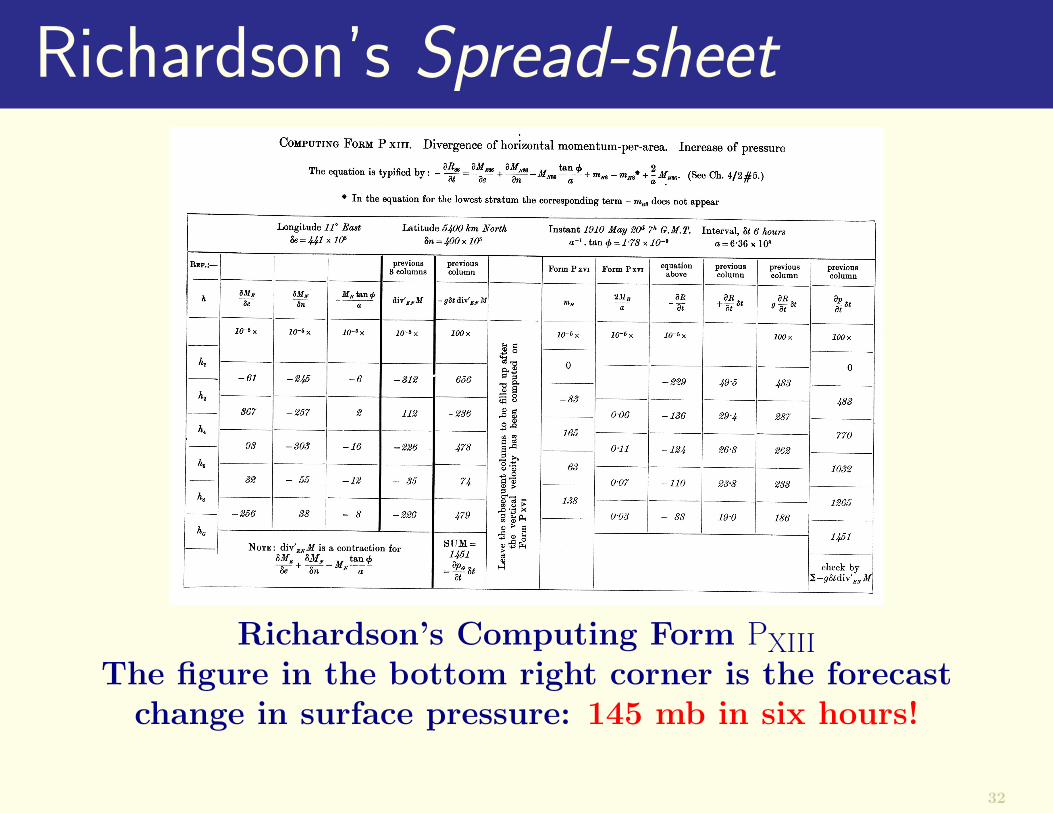
Richardson’s Spread-sheet
Richardson’s Computing Form PXIIIThe figure in the bottom right corner is the forecast
change in surface pressure: 145 mb in six hours!
32
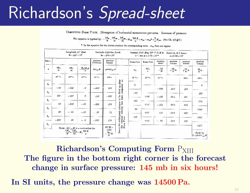
Richardson’s Spread-sheet
Richardson’s Computing Form PXIIIThe figure in the bottom right corner is the forecast
change in surface pressure: 145 mb in six hours!
In SI units, the pressure change was 14500Pa.32
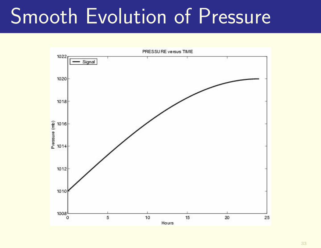
Smooth Evolution of Pressurex
33

Noisy Evolution of Pressurex
34

Tendency of a Smooth Signalx
35

Tendency of a Noisy Signalx
36

The Third Reading from
The Book of Limerick
37

The Third Reading from
The Book of Limerick
Young Richardson wanted to knowHow quickly the pressure would grow.
37

The Third Reading from
The Book of Limerick
Young Richardson wanted to knowHow quickly the pressure would grow.
But, what a surprise, ’cosThe six-hourly rise was,
37

The Third Reading from
The Book of Limerick
Young Richardson wanted to knowHow quickly the pressure would grow.
But, what a surprise, ’cosThe six-hourly rise was,
In Pascals, One Four Five Oh Oh!
37

Richardson’s Forecast Factory (A. Lannerback).Dagens Nyheter, Stockholm. Reproduced from L. Bengtsson, ECMWF, 1984
38

Richardson’s Forecast Factory (A. Lannerback).Dagens Nyheter, Stockholm. Reproduced from L. Bengtsson, ECMWF, 1984
64,000 Computers: The first Massively Parallel Processor38

Advances 1920–1950
�Dynamic Meteorology
� Rossby Waves
� Quasi-geostrophic Theory
� Baroclinic Instability
�Numerical Analysis
� CFL Criterion
�Atmopsheric Observations
� Radiosonde
�Electronic Computing
� ENIAC39

The ENIAC
40

Electronic Computer Project, 1946(under direction of John von Neumann)Von Neumann’s idea:Weather forecasting was a scientific problem par excellencefor solution using a large computer.
The objective of the project was to study the problem ofpredicting the weather by simulating the dynamics of theatmosphere using a digital electronic computer.
A Proposal for funding listed three “possibilities”:
1. Entirely new methods of weather prediction by calcula-tion will have been made possible;
2. A new rational basis will have been secured for the plan-ning of physical measurements and field observations;
3. The first step towards influencing the weather by rationalhuman intervention will have been made.
41

The ENIAC
The ENIAC (Electronic Nu-merical Integrator and Com-puter) was the first multi-purpose programmable elec-tronic digital computer.It had:
• 18,000 vacuum tubes
• 70,000 resistors
• 10,000 capacitors
• 6,000 switches
Power Consumption: 140 kWatts
42

The ENIAC: Technical Details.ENIAC was a decimal machine. No high-level language.Assembly language. Fixed-point arithmetic: −1 < x < +1.10 registers, that is,Ten words of high-speed memory.Function Tables:624 6-digit words of “ROM”, set onten-pole rotary switches.“Peripheral Memory”:Punch-cards.Speed: FP multiply: 2ms(say, 500 Flops).Access to Function Tables: 1ms.Access to Punch-card equipment:You can imagine!
43

Jule Charney found the solution to the noise problem: hederived the the Quasi-geostrophic equations.
The Q-geostrophic equations are a Filtered System.
They have solutions corresponding to “weather waves” butno solutions corresponding to “noise waves”.
? ? ?
44

Jule Charney found the solution to the noise problem: hederived the the Quasi-geostrophic equations.
The Q-geostrophic equations are a Filtered System.
They have solutions corresponding to “weather waves” butno solutions corresponding to “noise waves”.
? ? ?
Evolution of the Project:
• Plan A: Integrate the Primitive Equations
Problems similar to Richardson’s would arise
• Plan B: Integrate baroclinic Q-G System
Too computationally demanding
• Plan C: Solve barotropic vorticity equation
Very satisfactory initial results
44

The Fourth Reading from
The Book of Limerick
45

The Fourth Reading from
The Book of Limerick
Jule Charney was quite philosophic:“The system called Q-geostrophic,
45

The Fourth Reading from
The Book of Limerick
Jule Charney was quite philosophic:“The system called Q-geostrophic,
With filtered equationsSans fast oscillations,
45

The Fourth Reading from
The Book of Limerick
Jule Charney was quite philosophic:“The system called Q-geostrophic,
With filtered equationsSans fast oscillations,
Will obviate trends catastrophic”.
45

Charney, Fjørtoft, von Neumann
46

Charney, et al., Tellus, 1950.[Absolute
Vorticity
]=
[Relative
Vorticity
]+
[Planetary
Vorticity
]η = ζ + f .
The atmosphere is treated as a single layer, and the flow isassumed to be nondivergent. Absolute vorticity is conservedfollowing the flow.
d(ζ + f )
dt= 0.
This equation looks deceptively simple. But it is nonlinear:
∂ζ
∂t+ V · ∇(ζ + f ) = 0 .
Or, in more detail:
∂
∂t∇2ψ +
{∂ψ
∂x
∂∇2ψ
∂y− ∂ψ
∂y
∂∇2ψ
∂x
}+ β
∂ψ
∂x= 0 ,
47

Solution method for BPVE∂ζ
∂t= −J(ψ, ζ + f )
1. Compute Jacobian
2. Step forward (Leapfrog scheme)
3. Solve Poisson equation for ψ (Fourier expansion)
4. Go to (1).
• Timestep : ∆t = 1 hour (2 and 3 hours also tried)
• Gridstep : ∆x = 750 km (approximately)
• Gridsize : 18 x 15 = 270 points
• Elapsed time for 24 hour forecast: About 24 hours.
Forecast involved punching about 25,000 cards. Most of theelapsed time was spent handling these.
48

ENIAC Algorithm
49

ENIAC: First Computer Forecast
50

Richardson’s reaction
�“Allow me to congratulate you and yourcollaborators on the remarkable progresswhich has been made in Princeton.
�“This is . . . an enormous scientific ad-vance on the single, and quite wrong,result in which Richardson (1922) ended.”
51

The Fifth Reading from
The Book of Limerick
52

The Fifth Reading from
The Book of Limerick
Old Richardson’s fabulous notionOf forecasting turbulent motion
52

The Fifth Reading from
The Book of Limerick
Old Richardson’s fabulous notionOf forecasting turbulent motion
Seemed totally off-the-track,
52

The Fifth Reading from
The Book of Limerick
Old Richardson’s fabulous notionOf forecasting turbulent motion
Seemed totally off-the-track,But then came the ENIAC,
To model the air and the ocean.
52

NWP OperationsThe Joint Numerical Weather Prediction (JNWP) Unit was
established on July 1, 1954:
�Air Weather Service of US Air Force
�The US Weather Bureau
�The Naval Weather Service.
Operational numerical forecasting began on 15 May, 1955,using a three-level quasi-geostrophic model.
53
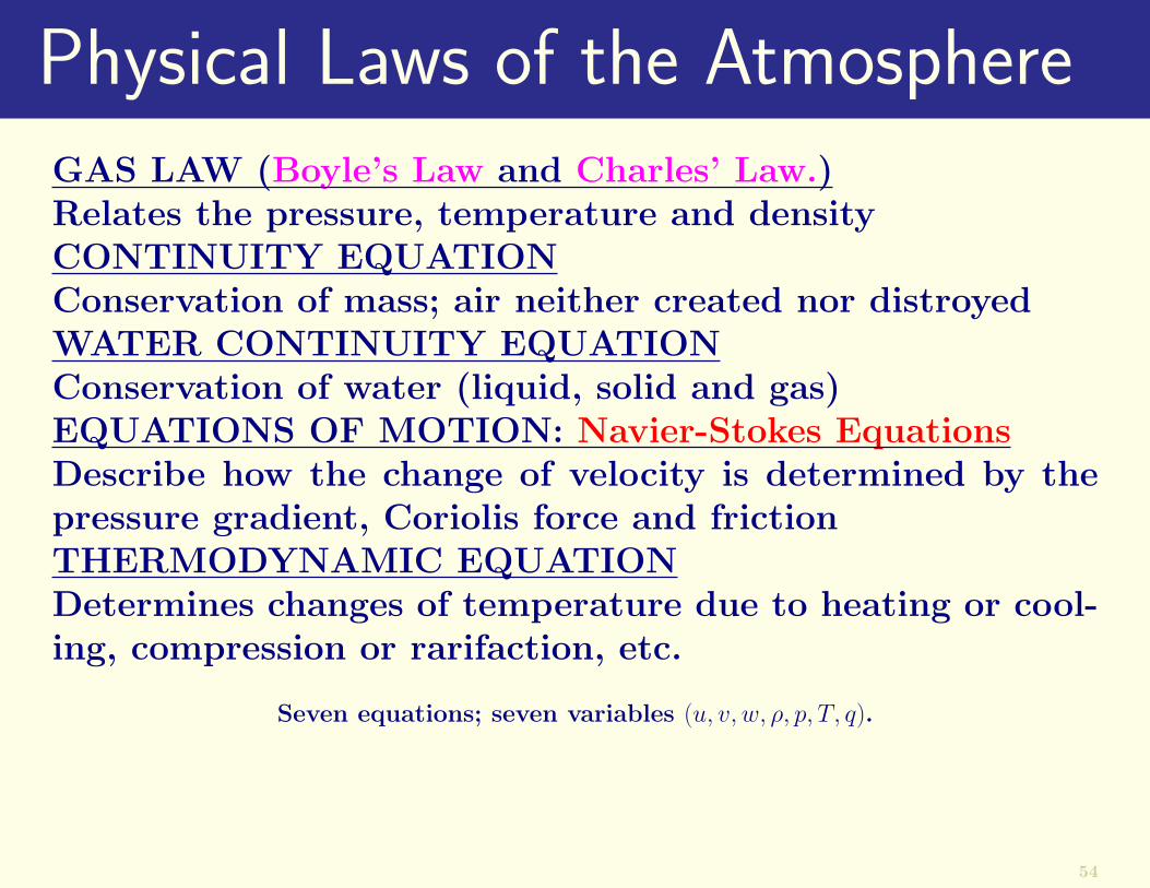
Physical Laws of the AtmosphereGAS LAW (Boyle’s Law and Charles’ Law.)Relates the pressure, temperature and densityCONTINUITY EQUATIONConservation of mass; air neither created nor distroyedWATER CONTINUITY EQUATIONConservation of water (liquid, solid and gas)EQUATIONS OF MOTION: Navier-Stokes EquationsDescribe how the change of velocity is determined by thepressure gradient, Coriolis force and frictionTHERMODYNAMIC EQUATIONDetermines changes of temperature due to heating or cool-ing, compression or rarifaction, etc.
Seven equations; seven variables (u, v, w, ρ, p, T, q).
54

The Primitive Equations
du
dt−
(f +
u tanφ
a
)v +
1
ρ
∂p
∂x+ Fx = 0
dv
dt+
(f +
u tanφ
a
)u +
1
ρ
∂p
∂y+ Fy = 0
p = RρT∂p
∂y+ gρ = 0
dT
dt+ (γ − 1)T∇ ·V =
Q
cp∂ρ
∂t+∇ · ρV = 0
∂ρw∂t
+∇ · ρwV = [Sources− Sinks]
Seven equations; seven variables (u, v, w, p, T, ρ, ρw).
55

Scientific Weather Forecasting in a Nut-Shell
• The atmosphere is a physical system
• Its behaviour is governed by the laws of physics
• These laws are expressed quantitatively in the form ofmathematical equations
• Using observations, we can specify the atmospheric stateat a given initial time: “Today’s Weather”
• Using the equations, we can calculate how this state willchange over time: “Tomorrow’s Weather”
56

Scientific Weather Forecasting in a Nut-Shell
• The atmosphere is a physical system
• Its behaviour is governed by the laws of physics
• These laws are expressed quantitatively in the form ofmathematical equations
• Using observations, we can specify the atmospheric stateat a given initial time: “Today’s Weather”
• Using the equations, we can calculate how this state willchange over time: “Tomorrow’s Weather”
• The equations are very complicated (non-linear) and apowerful computer is required to do the calculations
• The accuracy decreases as the range increases; there isan inherent limit of predictibility.
56

Progress in numerical weather prediction overthe past fifty years has been quite dramatic.
Forecast skill continues to increase.
57

Progress in numerical weather prediction overthe past fifty years has been quite dramatic.
Forecast skill continues to increase.
However, there is a limit . . .57
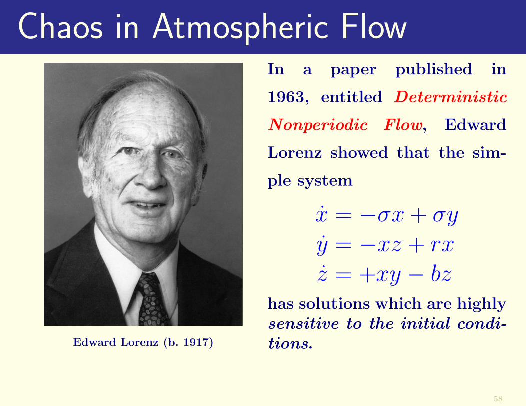
Chaos in Atmospheric Flow
Edward Lorenz (b. 1917)
In a paper published in
1963, entitled Deterministic
Nonperiodic Flow, Edward
Lorenz showed that the sim-
ple system
x = −σx + σyy = −xz + rxz = +xy − bz
has solutions which are highlysensitive to the initial condi-tions.
58
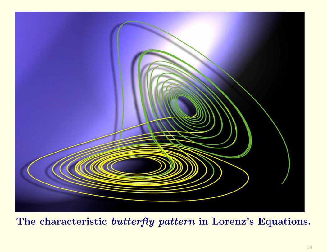
The characteristic butterfly pattern in Lorenz’s Equations.
59

Lorenz’s work demonstrated the practical impossibility ofmaking accurate, detailed long-range weather forecasts.
This problem can be traced back to Poincare, but it wasLorenz who formulated it in precise, quantitative terms.
60
Lorenz’s work demonstrated the practical impossibility ofmaking accurate, detailed long-range weather forecasts.
This problem can be traced back to Poincare, but it wasLorenz who formulated it in precise, quantitative terms.
In his 1963 paper he wrote:
“. . . one flap of a sea-gull’s wings may foreverchange the future course of the weather.”
Within a few years, he had changed species:
“Predictability:does the flap of a butterfly’s wings inBrazil set off a tornado in Texas?”
[Title of a lecture at an AAAS conference in Washington.]
60

The Sixth Reading from
The Book of Limerick
61

The Sixth Reading from
The Book of Limerick
Lorenz demonstrated, with skill,The chaos of heat-wave and chill:
61

The Sixth Reading from
The Book of Limerick
Lorenz demonstrated, with skill,The chaos of heat-wave and chill:
Tornadoes in TexasAre formed by the flexes
Of butterflies’ wings in Brazil.
61

Flow-dependent PredictabilityWeather forecasts lose skill because of the growth of er-rors in the initial conditions (initial uncertainties) and be-cause numerical models describe the atmosphere only ap-proximately (model uncertainties).
62

Flow-dependent PredictabilityWeather forecasts lose skill because of the growth of er-rors in the initial conditions (initial uncertainties) and be-cause numerical models describe the atmosphere only ap-proximately (model uncertainties).
As a further complication, predictability is flow-dependent.
The Lorenz model illustrates variations in predictability for different initial conditions.
62

63

Spaghetti plots for ensembles from two starting times.
64

Ensemble ForecastingIn recognition of the chaotic nature of the atmosphere, focushas now shifted to predicting the probability of alternativeweather events rather than a single outcome.
65

Ensemble ForecastingIn recognition of the chaotic nature of the atmosphere, focushas now shifted to predicting the probability of alternativeweather events rather than a single outcome.
The mechanism is the Ensemble Prediction System (EPS)and the world leader in this area is the European Centre forMedium-range Weather Forecasts (ECMWF).
65
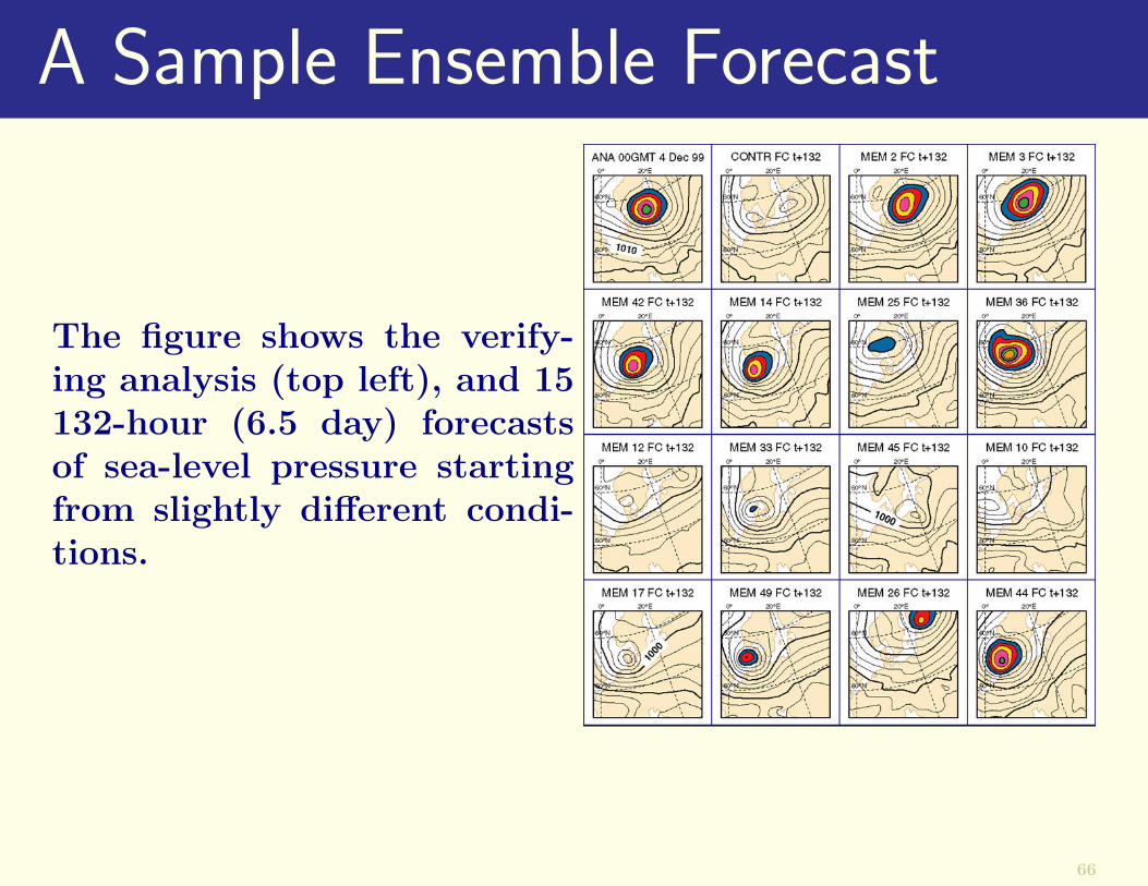
A Sample Ensemble Forecast
The figure shows the verify-ing analysis (top left), and 15132-hour (6.5 day) forecastsof sea-level pressure startingfrom slightly different condi-tions.
66

Ensemble of fifty forecasts from ECMWF.
These products are produced routinely and used operationally in the member states.
67
The Seventh (and last) Reading
from The Book of Limerick
68

The Seventh (and last) Reading
from The Book of Limerick
If errors still bother you, Tough!Uncertainty is The Right Stuff.
68

The Seventh (and last) Reading
from The Book of Limerick
If errors still bother you, Tough!Uncertainty is The Right Stuff.
It’s anyone’s guess,So use E-P-S,
From E-C-M-Double-you-uhf.
68

Thank you
69