a cognitive fault diagnosis system for sensor networks · santi: un sistema di monitoraggio...
TRANSCRIPT

POLITECNICO DI MILANODIPARTIMENTO DI ELETTRONICA, INFORMAZIONE E BIOINGEGNERIA
DOTTORATO DI RICERCA IN INGEGNERIA DELL’INFORMAZIONE
A COGNITIVE FAULT DETECTION AND
DIAGNOSIS SYSTEM FOR SENSOR NETWORKS
Doctoral Dissertation of:Francesco Trovò
Supervisor:Prof. Manuel RoveriCo-supervisor:Prof. Cesare AlippiTutor:Prof. Francesco AmigoniThe Chair of the Doctoral Program:Prof. Carlo Ettore Fiorini
2014 – Cycle XXVII


Abstract
COGNITIVE fault detection and diagnosis systems represent a novelclass of systems, which are able to detect and diagnose faults bycharacterizing the functional relationships existing among datas-
treams and by learning the nominal conditions and the fault dictionary dur-ing the operational life directly from incoming data. These abilities makethe use of these systems particularly suitable for the field of sensor net-works, where no a priori information is generally available about the mon-itored process and the possibly occurring faults. Moreover, these sensornetworks generally work in harsh environmental conditions, thus the oc-currence of faults, degradation effects and ageing effects in their units andsensors are likely to happen. It is of paramount importance to detect anddiagnose such anomalous working conditions of sensor networks.
This dissertation introduces a novel Cognitive Fault Detection and Di-agnosis System for sensor networks, able to characterize the nominal stateof the process by relying on a fault-free dataset, detect and diagnose faultsas soon as they appear and learn in an on-line manner the set of possi-ble faults. To the best of our knowledge, we propose the first completeCognitive Fault Detection and Diagnosis System where the cognitive ap-proach is applied to all its phases: detection, isolation and identification.The proposed system is based on a theoretically grounded statistical frame-work, able to characterize the functional relationships existing among theacquired datastreams by relying on their modeling in the space of the pa-rameters. As a basis for the detection and diagnosis phases, the proposedsystem is able to learn a dependency graph, which models the functional
I

relationships existing among the acquired data. The detection phase is per-formed by analysing the variation of these functional relationships, througha Hidden Markov Model statistical modeling of the nominal state in the pa-rameter space of linear discrete time dynamic systems approximating mod-els. By considering a logic partition of the learned dependency graph, theproposed system is able to isolate the possible occurring faults, through theanalysis of the statistical behaviour of multiple relationships. The identifi-cation phase is performed by means of a novel evolving clustering-labelingalgorithm specifically designed for this task, which is also capable of learn-ing the fault dictionary in an on-line manner.
The proposed Cognitive Fault Detection and Diagnosis System has beenvalidated in a wide experimental campaign on both synthetic data and tworeal-world challenging and valuable applications: an environmental mon-itoring application for rock collapse and landslide forecasting system anda water network distribution monitoring system. The experimental results,compared with state of the art methods in the field, provided evidence forthe better detection and diagnostic abilities of the proposed Cognitive FaultDetection and Diagnosis System.
II

Sommario
ISistemi cognitivi per la rilevamento e la diagnosi di guasti sono una nuo-va classe di sistemi, che rilevano e diagnosticano guasti grazie alla ca-ratterizzazione delle relazioni funzionali esistenti tra le stream di dati:
essi apprendono le condizioni nominali e il dizionario dei guasti durante laloro vita operativa direttamente dai dati raccolti. Queste caratteristiche ren-dono l’utilizzo di questi sistemi particolarmente adatto allo scenario dellereti di sensori, dove solitamente non sono disponibili informazioni a priorirelative al processo monitorato e ai guasti che possono presentarsi. Inoltre,le reti di sensori operano in condizioni ambientali sfavorevoli, il che implicache guasti, effetti dovuti all’usura e effetti di invecchiamento si presentinodi frequente nelle loro unità o nei sensori.
Questa tesi di dottorato introduce un nuovo Sistema di Rilevamento e diDiagnosi di Guasti Cognitivo per reti di sensori, capace di caratterizzare lostato nominale del processo basandosi su di un set di dati privo di guasti,di rilevare e diagnosticare guasti non appena essi si presentano e di appren-dere on-line l’insieme dei possibili guasti. Proponiamo il primo Sistema diRilevamento e di Diagnosi di Guasti Cognitivo in cui l’approccio cognitivoè stato utilizzato in tutte le sue fasi: rilevamento, isolamento ed identifica-zione. Il sistema proposto è basato su un solido approccio statistico, checaratterizza le relazioni funzionali esistenti tra le stream di dati grazie allaloro modellizzazione nello spazio dei parametri dei sistemi dinamici linearia tempo discreto che le approssimano. Alla base delle fasi di rilevamen-to e diagnosi, il sistema proposto apprende un grafo delle dipendenze, chemodellizza le relazioni funzionali esistenti tra le stream di dati. La fase di
III

rilevamento dei guasti si basa sull’analisi della variazione delle relazionifunzionali considerate nella fase precedente, che viene rilevata grazie allamodellizzazione statistica dello stato nominale fornita dagli Hidden Mar-kov Model. Grazie alla partizione logica del grafo delle dipendenze edall’analisi statistica del comportamento di tutte le relazioni funzionali con-siderate, il sistema proposto riesce inoltre ad isolare il guasto. La fase diidentificazione del guasto viene svolta da un innovativo algoritmo di clu-stering evolutivo, il quale è in grado di apprendere on-line il dizionario deiguasti.
Il Sistema di Rilevamento e di Diagnosi di Guasti Cognitivo proposto èstato validato in un’estesa campagna sperimentale, che ha considerato siadati sintetici, sia dati generati da due applicazioni particolarmente interes-santi: un sistema di monitoraggio ambientale per la predizione di frane edun sistema di monitoraggio di una rete di distribuzione idrica. I risultatisperimentali ottenuti dal Sistema di Rilevamento e di Diagnosi di GuastiCognitivo proposto sono stati confrontati con quelli dei metodi nello sta-to dell’arte nel campo considerato e hanno dimostrato di ottenere miglioriperformance in termini di rilevamento e di diagnosi dei guasti.
IV

Contents
1 Introduction 11.1 Detection and Diagnosis of Faults in Sensor Networks . . . 3
1.1.1 Fault Detection . . . . . . . . . . . . . . . . . . . . 71.1.2 Fault Diagnosis . . . . . . . . . . . . . . . . . . . . 11
1.2 Cognitive Fault Detection and Diagnosis Systems . . . . . . 111.3 Original Contribution . . . . . . . . . . . . . . . . . . . . . 161.4 Dissertation Structure . . . . . . . . . . . . . . . . . . . . . 17
2 Problem Formulation 192.1 Sensor Network Measurements . . . . . . . . . . . . . . . . 192.2 Fault Modeling . . . . . . . . . . . . . . . . . . . . . . . . 212.3 Modeling the Faulty System . . . . . . . . . . . . . . . . . 232.4 Examples of Faults . . . . . . . . . . . . . . . . . . . . . . 262.5 Purposes of Fault Detection and Diagnosis . . . . . . . . . . 30
3 The Proposed Cognitive Fault Detection and Diagnosis System 333.1 General Architecture . . . . . . . . . . . . . . . . . . . . . 353.2 Dependency Graph . . . . . . . . . . . . . . . . . . . . . . 363.3 Modeling Functional Relationships Between Pairs of Sensors 383.4 Feature in the Parameter Space . . . . . . . . . . . . . . . . 423.5 The Phases of the Proposed Cognitive Fault Detection and
Diagnosis System (CFDDS) . . . . . . . . . . . . . . . . . 433.5.1 Graph Learning . . . . . . . . . . . . . . . . . . . . 433.5.2 Detection . . . . . . . . . . . . . . . . . . . . . . . . 44
V

Contents
3.5.3 Isolation . . . . . . . . . . . . . . . . . . . . . . . . 443.5.4 Identification . . . . . . . . . . . . . . . . . . . . . . 44
4 Dependency Graph Learning 474.1 Modeling the Relationship Between a Couple of Datastreams 484.2 Creating the Granger-based Dependency Graph . . . . . . . 51
5 Fault Detection 555.1 Fault Detection in the Parameter Space . . . . . . . . . . . 565.2 Mahalanobis-based Detection . . . . . . . . . . . . . . . . 575.3 Hidden Markov Model Change Detection Test . . . . . . . . 615.4 Ensemble Approach to Hidden Markov Model-Change De-
tection Test (HMM-CDT) . . . . . . . . . . . . . . . . . . 64
6 Fault Isolation 716.1 Cognitive Fault Isolation . . . . . . . . . . . . . . . . . . . 716.2 Fault Isolation Phase . . . . . . . . . . . . . . . . . . . . . 75
7 Fault Identification 797.1 Modeling the Nominal State . . . . . . . . . . . . . . . . . 807.2 On-line Modeling the Fault Dictionary . . . . . . . . . . . . 877.3 Dealing with Incipient Faults . . . . . . . . . . . . . . . . . 91
8 CFDDS Implementation 93
9 Experimental Results 979.1 The Considered Datasets . . . . . . . . . . . . . . . . . . . 97
9.1.1 Application D1: Synthetic Datasets . . . . . . . . . . 979.1.2 Application D2: Rialba Dataset . . . . . . . . . . . . 999.1.3 Application D3: Barcelona Water Distribution Net-
work System Dataset . . . . . . . . . . . . . . . . . 1009.2 Dependency Graph Learning . . . . . . . . . . . . . . . . . 100
9.2.1 Application D1: Synthetic Dataset . . . . . . . . . . 1029.2.2 Application D2: Rialba Dataset . . . . . . . . . . . . 107
9.3 Detection Phase . . . . . . . . . . . . . . . . . . . . . . . . 1089.3.1 Application D1: Synthetic Dataset . . . . . . . . . . 1099.3.2 Application D2: Rialba Dataset . . . . . . . . . . . . 113
9.4 Isolation Phase . . . . . . . . . . . . . . . . . . . . . . . . 1149.4.1 Application D3: Barcelona Water Distribution Net-
work System Dataset . . . . . . . . . . . . . . . . . 1169.5 Identification Phase . . . . . . . . . . . . . . . . . . . . . . 120
9.5.1 Application D1: Synthetic Dataset . . . . . . . . . . 123
VI

Contents
9.5.2 Application D2: Rialba Dataset . . . . . . . . . . . . 1309.5.3 Application D3: Barcelona Water Distribution Net-
work System Dataset . . . . . . . . . . . . . . . . . 1319.6 General Remarks . . . . . . . . . . . . . . . . . . . . . . . 133
10 Concluding Remarks 13510.1 Future Perspectives . . . . . . . . . . . . . . . . . . . . . . 137
Bibliography 143
Glossary 149
VII


CHAPTER1Introduction
Sensor networks represent an important and valuable technological solutionto monitor and acquire data from an environment, a critical infrastructureor a cyber-physical system. These data are generally used as input for anapplication, which is able to take a decision or react to the change in the in-spected system. Examples of these applications based on sensor networks,are those inspecting an environmental phenomenon (e.g., a river, a rockwall or a coral reef) protecting critical infrastructures or those monitoringthe behaviour of a water distribution network.
Sensor networks are composed by a set of sensing units, each of whichis composed by a set of sensors, a processing board and a data transferapparatus. Each unit is deployed in a different location in the area influ-enced by the inspected phenomenon and contains multiple sensors, eachof which gathers meaningful information about it. The measurements pro-vided by the sensors are homogeneous or heterogeneous, in the sense thatthey are measuring the same physical quantity or different but related phys-ical quantities. The processing boards are responsible for the processing ofthe acquired data and management of the units (e.g., they manage the sen-sors sampling synchronization and/or analog to digital conversion of thereceived signals). Finally, the data transferring apparatus sends acquired
1

Chapter 1. Introduction
data to a central processing station, where the data are stored and elabo-rated. During the operational life of this infrastructure, the sensor networkcontinuously inspects the system status, by sending measurements to thecentral processing station, where the application runs. In fact, based onmeasurements coming from the sensor network, applications can be de-signed to take decisions (e.g., in the case a deviation from the usual work-ing conditions is registered, an alarm is raised) and contextually react tothe change (e.g., for critical infrastructures, alert the population about theexpected threat).
In this scenario, a model for the inspected phenomenon is usually un-known and the assumption of process stationarity may not hold, even thoughthese assumptions would generally improve the decision abilities of theaforementioned applications. Thus, information coming from the sensornetwork is critical to monitor the underlying process, to check the status ofthe system and react according to its behaviour. For instance, even if themodeling of the processes affecting a rock wall is generally not feasible, aconstant monitoring action of cracks width and rock inclination measure-ments may predict if a collapse is likely to happen.
Sensor networks usually work in harsh real-working conditions, whichmay induce permanent or transient faults, thermal drifts or ageing affectsaffecting both the embedded electronic boards which manage the sensorsand the sensors themselves. In fact, both the electro-mechanical compo-nents and the embedded electronics of the sensors are affected by physi-cal degradation (due to e.g., humidity, dust, chemicals and electromagneticradiations), which may induce a gradual deviation of the measured valuefrom the real one. Moreover, problems may arise on the processing boards,which may convert data coming from sensors (e.g., from analog to digi-tal) in a incorrect way. Finally, a correct behaviour of the communicationapparatus is crucial for the collection of the measurements, since a degra-dation of the information carried by the transferred data may occur duringthe transmission phase, both if the channels are physical, e.g., if the cablesare not properly maintained, or if they are wireless, e.g., if an unexpectedperturbation influences the data transmission frequencies.
It is of paramount importance to promptly detect and diagnose faultsoccurring in a specific unit, since they could affect the application layer,which operates based on the assumption that information provided by thesensor network is not corrupted. If the application does not take into ac-count the possibility of a fault (i.e., it is not robust to faults), it may take anincorrect decision, e.g., not alert the population when a threat is present orvice versa. Moreover, the corruption of a single unit could spread through-
2
1.1. Detection and Diagnosis of Faults in Sensor Networks
out the entire network (domino or cascade effect), which could eventuallycompromise the effectiveness of the monitoring action, even in the part ofthe network which is working properly.
Moreover, in the sensor network scenario the unexpected deviation fromnominal conditions may be caused either by a fault or by a change in theinspected process. It is crucial to distinguish between these two situations:in the former case, direct maintenance should be performed, while the lat-ter one requires a reaction to an environmental change, specifically chosenbased on the considered application scenario. Thus, the objective of thisdissertation is twofold: at first, to be able to understand when the sensornetwork is changing and, after that, to distinguish between the change inthe environment and a fault affecting a sensing unit.
1.1 Detection and Diagnosis of Faults in Sensor Networks
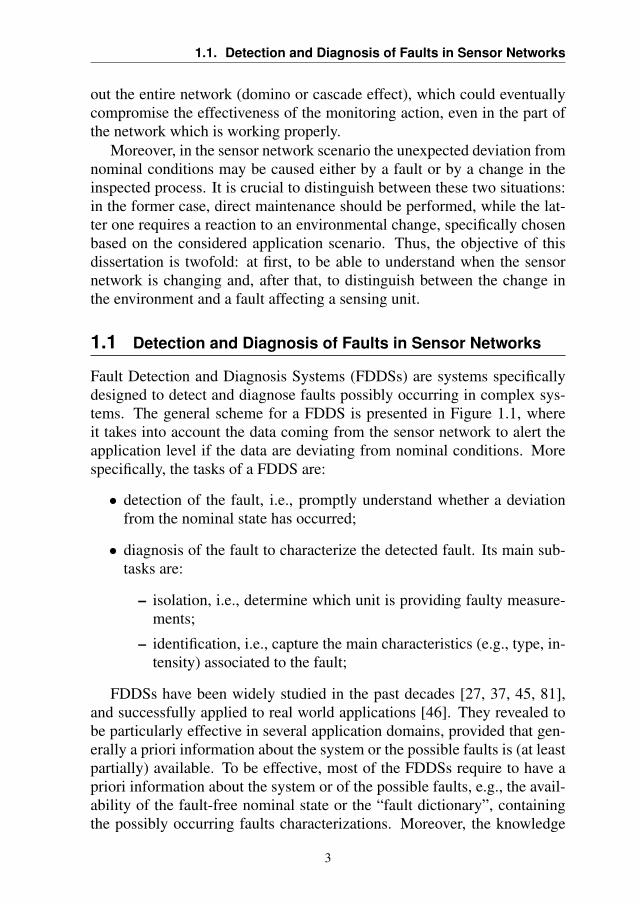
Fault Detection and Diagnosis Systems (FDDSs) are systems specificallydesigned to detect and diagnose faults possibly occurring in complex sys-tems. The general scheme for a FDDS is presented in Figure 1.1, whereit takes into account the data coming from the sensor network to alert theapplication level if the data are deviating from nominal conditions. Morespecifically, the tasks of a FDDS are:
• detection of the fault, i.e., promptly understand whether a deviationfrom the nominal state has occurred;
• diagnosis of the fault to characterize the detected fault. Its main sub-tasks are:
– isolation, i.e., determine which unit is providing faulty measure-ments;
– identification, i.e., capture the main characteristics (e.g., type, in-tensity) associated to the fault;
FDDSs have been widely studied in the past decades [27, 37, 45, 81],and successfully applied to real world applications [46]. They revealed tobe particularly effective in several application domains, provided that gen-erally a priori information about the system or the possible faults is (at leastpartially) available. To be effective, most of the FDDSs require to have apriori information about the system or of the possible faults, e.g., the avail-ability of the fault-free nominal state or the “fault dictionary”, containingthe possibly occurring faults characterizations. Moreover, the knowledge
3

Chapter 1. Introduction
Process/Phenomenon
Sensor Network
Fault detectionand diagnosis
Application
decision/reaction
Figure 1.1: General scheme of a monitoring system: it is able to inspect a process ora phenomenon with a sensor network. Data are gathered by sensors and transferredto an application which is able to take decision/reaction based on those data. A faultdetection and diagnosis system is critical to avoid that malfunctioning of the sensornetwork might induce an incorrect behaviour of the application.
4

1.1. Detection and Diagnosis of Faults in Sensor Networks
of the noise level (or the assumption of its absence) allows to have math-ematical models of dynamic processes by theoretical/physical modeling orby relying on system identification techniques. The knowledge of the faultdictionary and the noise level is hardly available in the sensor networksscenario, thus most of the traditional methods are not directly applicable inreal world sensor network applications.
5
Chapter 1. Introduction
FAU
LTD
ET
EC
TIO
NM
ET
HO
DS
data
-driv
ensi
gnal
-bas
ed
corr
elat
ion
spec
trum
anal
ysis
wav
elet
anal
ysis
mod
el-b
ased
para
m.
estim
atio
nne
ural
netw
orks
stat
eob
serv
ers
stat
ees
timat
ion
pari
tyeq
uatio
ns
Figu
re1.
2:Fa
ultd
etec
tion
taxo
nom
y
FAU
LTD
IAG
NO
SIS
ME
TH
OD
S
clas
sific
atio
nm
etho
ds
patte
rnre
cogn
ition
deci
sion
tabl
es
stat
istic
alcl
assi
ficat
ion
baye
scl
assi
fier
deci
sion
tree
appr
oxim
atio
nm
etho
ds
poly
nom
ial
clas
sifie
r
dens
ity-b
ased
met
hods
geom
etri
cal
clas
sifie
r
artifi
cal
inte
llige
nce
met
hods
fuzz
ycl
assi
fiers
neur
alne
tcl
assi
fier
infe
renc
em
etho
ds
bina
ryre
ason
ing
pred
icat
elo
gic
appr
oxim
ate
reas
onin
g
fuzz
ylo
gic
neur
alne
twor
ks
Figu
re1.
3:Fa
ultd
iagn
osis
taxo
nom
y
6

1.1. Detection and Diagnosis of Faults in Sensor Networks
Process ObservedBehaviour
NominalBehaviour
Comparison Detection
Figure 1.4: Generic fault detection scheme: the Process is characterized through its Nom-inal Behaviour. The Observed Behaviour is compared with the nominal one and, if adiscrepancy is assessed, the system detects a change
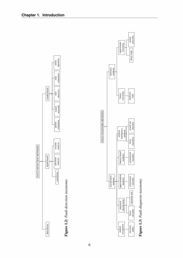
A taxonomy of the methods present in the literature of fault detectionand diagnosis systems, inspired by the one presented in [45], is provided inFigures 1.2 and 1.3, respectively.
1.1.1 Fault Detection
A general scheme for fault detection is depicted in Figure 1.4. This schemeis based on the knowledge of the nominal behaviour of the actual system,which is compared against the observed process behaviour. Usually, thecomparison is performed by inspecting features that reflect the discrepancybetween the two aforementioned behaviours. Different kinds of featurescan be encompassed. If we only have information about the characteristicvalue or behaviour of the chosen features in nominal conditions, limit ortrend checking is the most simple and frequently used method for changedetection. The measured values or trends (i.e., first derivatives) are mon-itored and checked to verify whether they exceed certain lower and up-per thresholds. If we consider a known distribution as the model for fea-tures, it is possible to check for some meaningful statistics by estimatingthe moments of the distribution (e.g., mean, variance, kurtosis). In thiscase, Change Detection Tests (CDTs) [21] can be considered to check forchanges in the distribution. This could be performed in an off-line way,through statistical tests, or by relying on sequential techniques, such ascontrol charts, which are able to verify whether a change in the data distri-bution has happened in an on-line manner. Most of the off-line and on-linetests present in literature require that the distribution of the data is fixed orknown. Finally, more complex methods for accounting for uncertainty inthe system are the ones which are based on the use of adaptive or fuzzythresholds.
The features considered in the change detection methods have different
7

Chapter 1. Introduction
Process Sensors Y
ε (Noise)
FeatureGeneration
ChangeDetection
NominalBehaviour
Features-Data-Trend
Change Fault
Figure 1.5: Data-driven scheme for fault detection in the sensor network scenario.
nature, which are based on the different models we may consider for thesignal generated from the process: the approaches are data-driven, signal-based and model-based, as described in Figure 1.2. They differ in the mod-eling approach used for the signal considered for fault detection. While thedata-driven approach does not assume any model for the incoming data, thesignal-based one makes use of the characteristics of the signal to provide adetection result. Finally, the model-based approach relies on the modelingof the process generating the data to detect changes. All the aforemen-tioned methods rely on one of the change detection techniques previouslydescribed to assess if a discrepancy between the expected and observedbehavior is present.
The first class of modeling approaches for fault detection is the data-driven one, which is based on the direct analysis of the provided measure-ments. This approach does not require the assumption of a specific modelfor the data generation procedure. Its generic scheme is presented in Fig-ure 1.5. The features which are monitored for fault detection purposes arethe measured variables or trends present in the data.
When a signal model for the data generation process is provided, faultdetection schemes as in Figure 1.6 can be adopted. If we consider the sig-nal as a stochastic process, we can consider as features statistics like sampleestimated moments (mean, variance or kurtosis) or autocorrelation. Thesestatistics can be used in the change detection framework on the hypothe-sis that the signal distribution is known and fixed over time. Otherwise, if
8

1.1. Detection and Diagnosis of Faults in Sensor Networks
Process Sensors Y
ε (Noise)
SignalModel
FeatureGeneration
ChangeDetection
NominalBehaviour
Signal-based faultdetection-Correlation function-Fourier analysis-Wavelet analysisFeatures-Exceeded threshold-Amplitudes-Frequencies
Change Fault
Figure 1.6: Signal-based scheme for fault detection in the sensor network scenario.
the signal presents periodic behaviours, techniques like bandpass filtering,Fourier analysis, correlation analysis and cepstrum analysis may be used toextract features. These techniques coupled with the aforementioned limitchecking methods can be used to detect changes in the signal. If the sta-tionarity assumption does not hold, short-time Fourier transform or wavelettransform could be performed to take into account local characteristics ofthe signal.
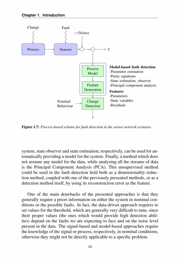
The third class of approaches to fault detection takes into account morethan one stream of data at a time to model the relationship between inputand output of a process, as depicted in Figure 1.7. Model-based meth-ods exploit the relationships existing among a set of measured variables toextract information about possible changes caused by faults. These meth-ods are based on different model identification techniques, both for linearand non-linear processes, like Least Square (LS) method, polynomial ap-proximators, Artificial Neural Networks (ANNs) and semi-physical mod-els. A widely known model-based method is the parity equations one: inthis paradigm the model behaviour in nominal conditions is compared withthe model during the operational life. This discrepancy, called residual, ischecked for consistency to provide a detection. In the case the process ischaracterized by a linear continuous and discrete-time state-space dynamic
9
Chapter 1. Introduction
Process Sensors Y
ε (Noise)
ProcessModel
FeatureGeneration
ChangeDetection
NominalBehaviour
Model-based fault detection-Parameter estimation-Parity equations-State estimation, observer-Principal component analysis
Features-Parameters-State variables-Residuals
Change Fault
Figure 1.7: Process-based scheme for fault detection in the sensor network scenario.
system, state observer and state estimation, respectively, can be used for au-tomatically providing a model for the system. Finally, a method which doesnot assume any model for the data, while analyzing all the streams of datais the Principal Component Analysis (PCA). This unsupervised methodcould be used in the fault detection field both as a dimensionality reduc-tion method, coupled with one of the previously presented methods, or as adetection method itself, by using its reconstruction error as the feature.
One of the main drawbacks of the presented approaches is that theygenerally require a priori information on either the system in nominal con-ditions or the possible faults. In fact, the data-driven approach requires toset values for the threshold, which are generally very difficult to tune, sincetheir proper values (the ones which would provide high detection abili-ties) depend on the faults we are expecting to face and on the noise levelpresent in the data. The signal-based and model-based approaches requirethe knowledge of the signal or process, respectively, in nominal conditions,otherwise they might not be directly applicable to a specific problem.
10
1.2. Cognitive Fault Detection and Diagnosis Systems
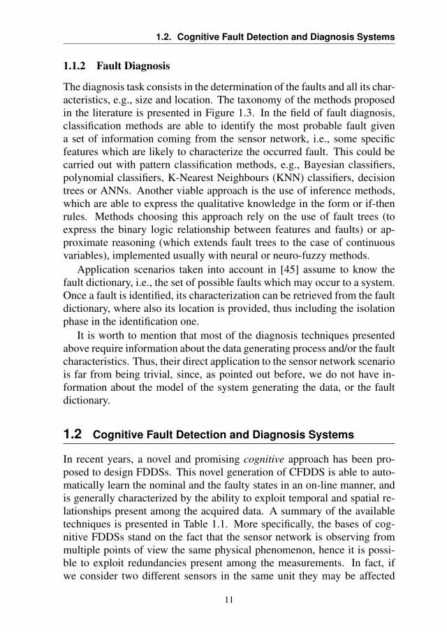
1.1.2 Fault Diagnosis
The diagnosis task consists in the determination of the faults and all its char-acteristics, e.g., size and location. The taxonomy of the methods proposedin the literature is presented in Figure 1.3. In the field of fault diagnosis,classification methods are able to identify the most probable fault givena set of information coming from the sensor network, i.e., some specificfeatures which are likely to characterize the occurred fault. This could becarried out with pattern classification methods, e.g., Bayesian classifiers,polynomial classifiers, K-Nearest Neighbours (KNN) classifiers, decisiontrees or ANNs. Another viable approach is the use of inference methods,which are able to express the qualitative knowledge in the form or if-thenrules. Methods choosing this approach rely on the use of fault trees (toexpress the binary logic relationship between features and faults) or ap-proximate reasoning (which extends fault trees to the case of continuousvariables), implemented usually with neural or neuro-fuzzy methods.
Application scenarios taken into account in [45] assume to know thefault dictionary, i.e., the set of possible faults which may occur to a system.Once a fault is identified, its characterization can be retrieved from the faultdictionary, where also its location is provided, thus including the isolationphase in the identification one.
It is worth to mention that most of the diagnosis techniques presentedabove require information about the data generating process and/or the faultcharacteristics. Thus, their direct application to the sensor network scenariois far from being trivial, since, as pointed out before, we do not have in-formation about the model of the system generating the data, or the faultdictionary.
1.2 Cognitive Fault Detection and Diagnosis Systems
In recent years, a novel and promising cognitive approach has been pro-posed to design FDDSs. This novel generation of CFDDS is able to auto-matically learn the nominal and the faulty states in an on-line manner, andis generally characterized by the ability to exploit temporal and spatial re-lationships present among the acquired data. A summary of the availabletechniques is presented in Table 1.1. More specifically, the bases of cog-nitive FDDSs stand on the fact that the sensor network is observing frommultiple points of view the same physical phenomenon, hence it is possi-ble to exploit redundancies present among the measurements. In fact, ifwe consider two different sensors in the same unit they may be affected
11

Chapter 1. Introduction
by a parasitic effect (e.g., dependence from temperature), thus providingtemporal redundant data. Similarly, if we consider two sensors in differentunits providing homogeneous measurements we are able to infer if the phe-nomenon is affecting both the locations in the same way, i.e., if a spatialredundancy or causality is present. The learned relationships among sensormeasurements are used to detect whether the data are deviating from thenominal behaviour and, possibly, diagnose the causes of this deviation.
12

1.2. Cognitive Fault Detection and Diagnosis Systems
Tabl
e1.
1:R
elev
anta
ppro
ache
sin
Cog
nitiv
eF
DD
S
Cha
ract
eris
tics
Taxo
nom
yPa
per
Nom
inal
Stat
eFa
ultD
ictio
nary
App
licat
ion
Det
ectio
nD
iagn
osis
[36]
Giv
enL
earn
edD
ynam
icsy
stem
sPa
rity
Equ
atio
nsN
eura
lNet
wor
ks[3
0]G
iven
(bou
nded
erro
r)L
earn
edD
ynam
icsy
stem
sSt
ate
estim
ator
N.a
.[8
0]G
iven
(bou
nded
erro
r)L
earn
edD
ynam
icsy
stem
sSt
ate
estim
ator
Ada
ptiv
efil
teri
ng[8
8]L
earn
edG
iven
Che
mic
alpr
oces
sN
eura
lNet
wor
ksN
eura
lNet
wor
ksC
lass
ifier
s[4
3]L
earn
edG
iven
Tran
sfor
mer
N.a
.N
eura
lNet
wor
ksC
lass
ifier
s[8
6]G
iven
On-
line
Ele
ctri
cM
otor
sN
.a.
Neu
ralN
etw
orks
Cla
ssifi
ers
[90]
Lea
rned
Giv
enSt
irre
dta
nkre
acto
rN
.a.
Neu
ro-F
uzzy
logi
c[6
1]L
earn
edG
iven
Bal
lbea
ring
sN
.a.
Neu
ro-F
uzzy
logi
c[7
7]L
earn
edG
iven
Indu
ctio
nM
otor
sN
.a.
Neu
ro-F
uzzy
logi
c[4
4]L
earn
edG
iven
Tran
sfor
mer
sN
.a.
Fuzz
ylo
gic
[64]
Lea
rned
Giv
enTr
ansf
orm
ers
N.a
.N
euro
-Fuz
zylo
gic
[57]
Lea
rned
Giv
enM
arin
epr
opul
sion
engi
neN
.a.
Neu
ro-F
uzzy
logi
c[4
9]L
earn
edG
iven
Gea
rbox
esN
eura
lNet
wor
ksN
.a.
[3]
Lea
rned
Giv
enC
ircu
ittr
ansm
issi
onN
.a.
AIM
etho
ds[2
6]L
earn
edL
earn
edD
ynam
icsy
stem
sM
odel
-Bas
edIn
fere
nce
met
hod
[8]
Lea
rned
Lea
rned
Dyn
amic
syst
ems
Dat
a-dr
iven
Infe
renc
em
etho
d
13
Chapter 1. Introduction
Cognitive approaches generally rely on Machine Learning (ML) tech-niques to configure the nominal state and characterize the faulty ones with-out requiring any a-priori information about the fault signature or of thefault time profile. The ancestors of this approach can be found in workspublished starting from the nineties. Most of these papers focus on specificapplications or provide algorithms which confine the cognitive approach toa specific phase. The idea behind cognitive FDDSs is suggested in [45],while most of the systematic research relying on this paradigm has beendeveloped in the last 2-3 years.
Most of existing cognitive FDDSs apply the learning mechanism onlyto a single aspect of the system [30, 36, 80], thus they still require at least toknow partial information about the analysed process. In more detail, [36]proposes a learning procedure for unanticipated fault accommodation, un-der the assumption that the process model is given. [30] presents a learningmethodology for incipient failure detection based on nonlinear on-line ap-proximators, which aims at both inspecting variations in the system due tofaults and provides information about the detected faults in an on-line man-ner. [80] extends the approach presented in [30], by coupling the on-lineapproximators with a learning procedure for the accommodation of schemeparameters.
There is a large literature addressing the design of cognitive FDDSsfor specific applications based on neural networks [43, 86, 88] and fuzzylogic [3, 44, 49, 57, 61, 64, 77, 90], with cognitive mechanisms mostly ap-plied during the training phase of the FDDS. For instance, [88] presents asupervised method for fault classification, which relies on the learning of aRadial Basis Function (RBF) network for chemical process modeling andfault detection, while a second neural network is used for fault identification(classification) task. [43] describes a FDDS specifically designed for faultidentification in power transformers based on genetic algorithms for train-ing a neural network. In [86], the authors propose an intelligent FDDS forelectric motors based on Adaptive Resonance Theory and Kohonen NeuralNetwork (ART-KNN): new faults can be included in the dictionary thanksto the design of a case-based reasoning system, where faults are reportedby experts and automatically included in the system. [90] suggests a faultidentification technique based on the joint use of fuzzy logic and feedfor-ward neural networks, where the fuzzyfication logic is mainly based ona priori knowledge of the considered application, i.e., a stirred tank reac-tor. [61] proposes a classification method for faults occurring in ball bear-ing, which considers a wavelet analysis on the accelerometer measured sig-nals, whose results are feed to an Adaptive Network-based Fuzzy Inference
14
1.2. Cognitive Fault Detection and Diagnosis Systems
System (ANFIS) able to adapt to newly received signals. [77] presents anapproach for classification of faults affecting induction motors which re-lies on a combination of unsupervised and supervised learning to clusterand classify faulty patterns for the value of the current. [44] extends theusual dissolved gas analysis for transformer with an evolving programmingfuzzy-based approach for identifying incipient faults, presenting a geneticapproach to train the fuzzy rules used for classification. On the same appli-cation, in [64] a system based on subtractive clustering, as a basis for fuzzyrules creation and optimization, is proposed. In [57], a fault identificationsystem is proposed for the specific field of propeller-shaft marine propul-sion engine: a neuro-fuzzy system trained with genetic algorithms allowsto distinguish among a predefined set of faults. In [49], a fault detectionalgorithm for inspecting the frequency spectrum of vibration signals com-ing from gearboxes is presented. This method uses function fuzzy c-meansalgorithm to cluster spectra and detect if a fault is likely to arise. Finally,the problem of fault identification in circuit transmission is solved in [3] byusing fuzzy adaptive neural network, which are able to automatically learnthe fuzzy rules associated with a specified set of faults.
We would like to remark that, the solutions designed for specific appli-cations we mentioned above require supervised information on the faults,i.e., to know the fault dictionary. As mentioned before, the cognitive aspectof these methods is confined in the training phase, thus the characterizationof the nominal state is automatic, but information about the fault signatureis needed. Differently, [45] suggests the use of an unsupervised “clustering-labeling” method to automatically assign observations either to the nominalor the faulty classes, thus considering the possibility to improve the faultdictionary during the FDDS operational life. Unfortunately, no technicaldetails about the implementation of the solution are given.
Two works [8, 26], fully relying on the concept of cognitive, have beendeveloped in parallel with the work described in this dissertation. In [26]they propose a method for detection and identification of faults for genericunknown dynamic discrete-time systems, by relying on an approach basedon the analysis of the provided datastream in the functional space. Therequirement for training such FDDSs is a dataset composed entirely byfault-free instances of the dynamic system inspected by the sensor network.In [8] the fault detection problem is entailed by the use of Hidden MarkovModels (HMMs), which are able to model in a statistical way the nom-inal state of the system. Thanks to this characterization, they develop aHMM-CDT able to detect faults by inspecting the discrepancy of the faultydata from the nominal model learned by the HMM. More details about this
15

Chapter 1. Introduction
method will be provided in the sequel of this dissertation.
1.3 Original Contribution
In this dissertation we propose a new CFDDS meant to operate on sensornetworks. The proposed system is able to characterize the nominal condi-tions of the system, by relying on fault-free data coming from the sensornetwork. At first, the proposed system learns the dependency graph exist-ing among datastreams, to select only relevant functional relationships. Theanalysed relationships are able to capture the temporal and spatial redun-dancies present in the data. Based on them, the proposed CFDDS is ableto perform fault detection, isolation and identification, without requiring apriori information on either the inspected process or the faulty states.
To model the relationships constituting the causal dependency graph ofthe sensor network we rely on the concept of Granger causality, which al-lows to consider only those relationships providing meaningful informa-tion for fault detection and diagnosis. After learning the network depen-dency structure, fault detection and diagnosis is carried out in the spaceof estimated parameter vectors of Linear Time Invariant (LTI) models ap-proximating the functional relationships included in the dependency graph.Deviations from the learned nominal concept are detected by means of adecrease of the loglikelihood provided by the HMM modeling, which ishere considered to characterize the statistical pattern of the parameter vec-tors estimated on fault-free data (nominal state). Following the detectionphase, an isolation mechanism based on the logic partition of the depen-dency graph is able to distinguish between faults (whose location is alsoinferred) and change in the environment. Finally, in the case a fault hasoccurred, an identification procedure is executed to characterize and dis-criminate among different faults. The identification phase is performed bymeans of a newly developed evolving clustering-labeling technique in thespace of the parameter vectors. This framework was specifically designedfor fault diagnosis purposes and is able to learn the fault dictionary in anon-line manner.
The innovative aspects of this cognitive framework for fault detectionand diagnosis are:
• the design of a CFDDS completely based on the cognitive approach,relying on computational intelligence techniques, which is able tocover all the phases of fault detection and diagnosis in the sensor net-work scenario;
16

1.4. Dissertation Structure
• the development of a set of integrated techniques, coming from statis-tics and machine learning fields, which rely on a theoretically soundframework developed by the system identification field;
• the ability to characterize the temporal and spatial relationship exist-ing among data with the dependency graph, learned with the use of astatistical framework;
• the ability to characterize the nominal state of the system inspected bythe sensor network through learning mechanisms based on the cogni-tive approach;
• the ability to learn the fault dictionary during the operational life ofthe system, without requiring a priori information about the possiblefaults.
To validate the abilities of the proposed method we considered two realworld applications of environmental monitoring systems: the rock landslideand collapse forecasting system of the Rialba Towers in Northern Italy andthe Barcelona Water Network Distribution System (BWNDS). We took intoaccount these two relevant applications since, despite the lack of informa-tion about the data-generating process and their complexity, the cognitiveapproach is able to effectively address the problem of fault detection anddiagnosis.
1.4 Dissertation Structure
The dissertation is structured as follows: in Chapter 2 the mathematicalframework used in the sequel is presented, including the model of the con-sidered data-generating processes, the fault models and their influences onthe original process, as well as the purposes of the proposed framework.In Chapter 3, a general overview of the proposed system is presented, withparticular emphasis on the model approximation techniques adopted andon the theoretical results they rely on. Chapters 4 to 7 detail the graphlearning, the detection, isolation and identification phases adopted by theproposed CFDDS, respectively. Chapter 8 provides a brief overview of theimplementation of the developed techniques, while Chapter 9 describes thewide experimental campaign conducted to validate the performance of theproposed framework. Finally, in Chapter 10, some concluding remarks aredrawn, as well as future perspectives in the field.
17


CHAPTER2Problem Formulation
In this chapter, we provide a framework to formally describe data comingfrom a sensor network inspecting a process, whose model is unknown be-cause of the lack of information or because its modeling is too complex. To-wards this goal, in Section 2.1 we describe the model of the data generatingprocess we consider. A specification of the considered faults affecting thesensor network is provided in Section 2.2. Subsequently, in Section 2.3, wepresent the model of the sensor network during the faulty state. Then, someexamples of faults are presented in Section 2.4. Finally, the formulationof the problem of fault detection and diagnosis in the presented modelingframework is detailed in Section 2.5.
2.1 Sensor Network Measurements
We consider a time-invariant dynamic system P whose model descriptionis unavailable. A sensor network acquiring data from P is composed by aset of n ∈ N sensors:
S = s1, . . . , sn, (2.1)
where each sensor si acquires scalar measurements coming from P . Selec-tion of the most appropriate deployment positions for the sensors is outside
19

Chapter 2. Problem Formulation
the scope of this dissertation. The interested reader can refer to [33, 52,56, 71] for a comprehensive investigation of the placement problem. Theassumption of considering sensors providing scalar measurements may beovercome in a straightforward way. In fact, for a generic sensor si′ provid-ing d-variate measurements included in a network S ′, we can replace theoriginal sensor network with an equivalent one:
S ′ ← S ′ \ si′ ∪ s′1, . . . , s′d, (2.2)
where s′i are sensors providing as scalar measurement the i-th dimension ofthe measurement provided by si′ . This transformation allows us to considerin the sequel only scalar measurements coming from sensors.
We would like to point out that the sensors may observe both heteroge-neous or homogeneous physical quantities, e.g., sensors may provide tem-perature in different locations of the network (homogeneous measurements)or temperature and wind speed in the same one (heterogeneous measure-ments). All the sensors which are deployed in the same position belongsto a unit uj of the network or, more formally the network sensors can bepartitioned by a set of m ∈ N units:
U = u1, . . . , um, (2.3)
where each unit ui is a set of sensors ui ⊆ S and S =⋃i ui, ui ∩ uj =
∅, i 6= j.In the sequel we consider, for the sake of simplicity, sensor networks
where each unit is composed of a single sensor (m = n or ui = si ∀i)and where each sensor provides scalar measurements. Extensions to theCFDDS proposed in the following chapters are trivial.
We consider a sensor network that, through a suitable synchronizationalgorithm1, is able to provide at each time instant t ∈ N the measurementscolumn vector:
X(t) =
x1(t)...
xn(t)
∈ Rn, (2.4)
where xi(t) ∈ R is the scalar measurement acquired at time t by sensor si.By considering the entire monitoring period of the sensor network we
can define the datastream acquired by sensor si as:
xi = xi(t)t∈N (2.5)1The problem of measurements synchronization is out of the scope of this dissertation. The interested reader
can refer to [12].
20
2.2. Fault Modeling
and the multivariate vector containing datastreams xi as
X =
x1
...xn
. (2.6)
As final remark we would like to point out that in this dissertation we donot take into account continuous time dynamic processes, nor state-spaceformulations. In fact, for many applications of particular interest in thesensor networks field (e.g., environmental monitoring) we are interested inthe analysis of the discrete-time input-output relationships existing amongdatastreams [60].
2.2 Fault Modeling
In general, the behavior of the system under faulty conditions is not knowna priori, however, fault modeling is crucial in the design and analysis offault diagnosis schemes, since it allows to fully characterize a posteriorithe possible deviations occurring to the system. This section presents theoverall fault modeling framework that will be used during this dissertation.
Definition 2.2.1. A fault F (·) is defined as an unpermitted deviation ofat least one characteristic property or parameter of the system from theacceptable/usual/standard conditions. Formally, a fault F : N → R isrepresented as:
F (t) =ν∗∑ν=1
Bν(t; t(ν)i , t
(ν)f )φν(t), (2.7)
where:
• ν∗ is the number of time intervals where fault is present;
• Bν(t; t(ν)i , t
(ν)f ) ∈ [0, 1] denotes the time profile of the fault that occurs
at time instant t(ν)i and disappears at time instant t(ν)
f , with t(ν)f <
t(ν+1)i ;
• t(ν)i ∈ N and t(ν)
f ∈ N are the occurrence and disappearance time of
the fault in the ν-th time interval, respectively, with t(ν)i < t
(ν)f ;
• φν(t) ∈ R is the fault signature within the ν-th time interval at timeinstant t.
21

Chapter 2. Problem Formulation
The ν-th time profile Bν : N× N× N→ [0, 1] is described by:
Bν(t; ti, tf ) = β(ν)i (t− t(ν)
i )− β(ν)f (t− t(ν)
f ) (2.8)
where βi : Z → [0, 1] is the evolution mode of the fault occurrence fromtime t(ν)
i and βf : Z → [0, 1] is the evolution mode of disappearance fromtime t(ν)
f ,βi(t) = βf (t) = 0 ∀t < 0 (2.9)
andβ
(ν)i (t− t(ν)
i ) ≥ β(ν)f (t− t(ν)
f ) ∀t ∈ N. (2.10)
According to the time duration, a fault F can be characterized as [37,45]:
• intermittent (ν∗ > 1)
F (t) =ν∗∑ν=1
Bν(t; t
(ν)i , t
(ν)f
)φν (t) , (2.11)
• transient (ν∗ = 1, ∃ t ≤ ∞ s.t. βf (t) = 1 ∀t > t):
F (t) = B (t; ti, tf )φ(t), (2.12)
• permanent (ν∗ = 1, βf (t) = 0 ∀t ∈ N):
F (t) = B (t; ti, tf )φ(t), (2.13)
The time profile Bν (and thus the corresponding fault F ) can be charac-terized based on the evolution mode as:
• abrupt:
β(ν)k (t) =
0 t ≤ 0
1 t > 0(2.14)
• incipient:
β(ν)k (t) =
0 t ≤ 0
1− e−rkt t > 0(2.15)
where k ∈ i, f and ri and rf are the evolution rate of occurrenceand disappearance, respectively.
The fault signature φ(t) is usually a generic time varying scalar function.Here for modeling purposes, we specify some common faults:
22

2.3. Modeling the Faulty System
• constant:φ(t) = φ, φ ∈ R; (2.16)
• drift (linear):φ(t) = Rt, R ∈ R (2.17)
• precision degradation:φ(t) ∼ D(t), (2.18)
whereD(t) is a distribution of a stochastic process, such that E[D(t)] =0.
A graphical representation of the fault models is shown in Figure 2.1. Inthe case of intermittent faults, only the abrupt evolution mode of occurrenceand disappearance is depicted. In the general case, for each time interval offault presence, the evolution mode may be either abrupt or incipient.
In this dissertation, the assumption that data are continuously recorded,without any hole, is considered. Otherwise, while modeling faults weshould take into account the possibility that for some time period [ti; tf ]data are not coming from the sensor network, which is usually addressedas missing data fault. If it is the case and the period is relatively short, it ispossible to adopt reconstruction techniques as described in [13, 14, 69]. Ifthe fault period is too long such techniques are not viable anymore, sincetheir reconstruction error may explode with the progressing of time.
2.3 Modeling the Faulty System
Once the model for a fault F is specified, we need to determine how it af-fects the measurements coming from the sensor network S. A monitoringsystem subject to a fault F is presented in Figure 2.2. Under healthy condi-tions, the output of the sensor network at time t is the measurement columnvector X(t). The faults are usually represented either by external signalsor as parameter deviations and are induced in an additive and/or multiplica-tive way. The output of the sensor network at time t under faulty conditionsXF (t) is described by the following equations:
XF (t) = [In + Γ(t)]X(t) + Φ(t) (2.19)
where In is the identity matrix of order n, Γ(t) ∈ Rn×n is the multiplicativematrix at time t and Φ(t) ∈ Rn is the additive column vector at time t,modeling the effects of faults on the system. Γ(t) is a diagonal matrix suchthat each diagonal element [Γ(t)]ii = γii(t) is a fault γii(t) = Fi(t) with
23

Chapter 2. Problem Formulation
Fault signatureOffset Drift Precision Degradation
Inte
rmitt
ent
Abr
uptA
brup
t
F (t)
t
F (t)
t
F (t)
t
Tran
sien
t Abr
uptA
brup
t
F (t)
t
F (t)
t
F (t)
t
Abr
upt
Inci
pien
t F (t)
t
F (t)
t
F (t)
t
Inci
pien
tAbr
upt
F (t)
t
F (t)
t
F (t)
t
Inci
pien
tIn
cipi
ent F (t)
t
F (t)
t
F (t)
t
Perm
anen
t Abr
upt
F (t)
t
F (t)
t
F (t)
t
Inci
pien
t
F (t)
t
F (t)
t
F (t)
t
Figure 2.1: Specification of the faults considered in this dissertation. For the sake ofconcision we depicted only abrupt intermittent faults.
24

2.3. Modeling the Faulty System
Process/Phenomenon
Sensor Network
Fault Detectionand Diagno-sis System
Application
decision/reaction
Fault
X
XF (t)
F
Figure 2.2: Fault monitoring system: when a fault F occurs, the measurements providedby the sensor network XF are not describing the behaviour of the underlying sys-tem/phenomenon, given by X , i.e., XF 6= X . FDDSs are required to detect if thisdeviation from nominal condition occurs and to gather information about its causes.
25

Chapter 2. Problem Formulation
specific time profile and signature. The same applies to all the elements inΦ(t), i.e., [Φ(t)]j = φj(t) = Fj(t).
On the basis of the above definition we can define two different classesof faults affecting a system: additive and multiplicative.
Definition 2.3.1. An additive fault at time t affecting a sensor network pro-viding X(t) is defined by Γ(t) = 0 (null matrix of order n) and φ(t) 6= 0,i.e.,
XF (t) = X(t) + Φ(t). (2.20)
Definition 2.3.2. A multiplicative fault at time t affecting a sensor networkproviding X(t) is defined by Γ(t) 6= 0 and φ(t) = 0, i.e.,
XF (t) = [In + Γ(t)]X(t). (2.21)
There exist also some kind of faults which cannot be categorized intothe two definitions presented above. For instance, a commonly occurringfault is the stuck-at, which results in the freezing of the measurement ofa sensor on a single value over time, can be modeled as Γ(t) = −In andΦ(t) = C, C ∈ Rn, i.e., resulting in:
XF (t) = C. (2.22)
2.4 Examples of Faults
In the sequel, we present some examples of faults affecting a system: eachfault is coupled with a real one occurring in a sensor network designed toforecast rock landslides and collapses deployed at the Towers of Rialba, inNorthern Italy.
Additive Permanent Fault Here we want to model an additive permanentfault which occurs in a sensor network composed of n = 3 univariate sen-sors S = s1, s2, s3. The fault is influencing only the data coming fromthe third sensor s3, occurs at time ti with an abrupt profile and has an un-known profile µ(t). This fault models the introduction of a dynamic signalin the nominal behaviour of the sensor, which could be due to an externalcause. By following the modeling we presented in Section 2.2 we have:
26

2.4. Examples of Faults
Figure 2.3: Fault affecting the mounting of units on the rock face; only one of the signalsis affected.
Multiplicative Γ(t) =
0 0 0
0 0 0
0 0 0
;
Additive Φ(t) =
0
0
F (t)
;
Fault F (t) = B(t; ti, tf )φ(t);
Time signature B(t; ti, tf ) = βi(t− ti)− 0 =
0, t ≤ 0
1, t > ti;
Profile φ(t) = µ(t).
By observing the data acquired by an accelerometer, shown in Fig-ure 2.3, one may observe that the fault occurring at time ti = 7 has thetime profile and signature described above. The anomalous behaviour ofthe signal in the figure is classified as a fault since it is strange that an accel-eration coming from the inside affects only one of the axes whereas, apartfrom very particular situations, all axes should be affected. The rationale
27
Chapter 2. Problem Formulation
Figure 2.4: Thermal drift affecting a MEMS tiltmeter. The reading should be constant butthe thermal parasitic effects affect the measurements.
behind the generation of this accelerometer signature is currently unknown,however, we give the following most likely interpretation: the fault appearsto be associated with a movement of the nogs and screws system fixingthe monitoring unit to the rock. The movement is probably induced by thefreezing of the water present in the inner part of the drilled hole which, inturn, pushes the unit outside.
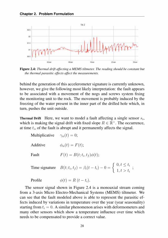
Thermal Drift Here, we want to model a fault affecting a single sensor si,which is making the signal drift with fixed slope R ∈ R+. The occurrence,at time ti, of the fault is abrupt and it permanently affects the signal.
Multiplicative γii(t) = 0;
Additive φii(t) = F (t);
Fault F (t) = B(t; ti, tf )φ(t);
Time signature B(t; ti, tf ) = βi(t− ti)− 0 =
0, t ≤ ti
1, t > ti;
Profile φ(t) = R (t− ti).
The sensor signal shown in Figure 2.4 is a monoaxial stream comingfrom a 3-axis Micro Electro-Mechanical Systems (MEMS) tiltmeter. Wecan see that the fault modeled above is able to represent the parasitic ef-fects induced by variations in temperature over the year (year seasonality)starting from ti = 0. A similar phenomenon arises with deformometers andmany other sensors which show a temperature influence over time whichneeds to be compensated to provide a correct value.
28

2.4. Examples of Faults
Figure 2.5: A low-probability intermittent fault at software level
Intermittent faults Finally we model an intermittent fault composed by v∗ =2 time intervals. Both the portions of the fault occur and disappear in anabrupt way and has a fixed magnitude θ ∈ R. Its modeling in the proposedframework is:
Multiplicative γii(t) = 0;
Additive φi(t) = F (t);
Fault F (t) =∑2
ν=1Bν(t; t(ν)i , t
(ν)f )φν(t− t(ν)
i );
Time signature Bν(t; t(ν)i , t
(ν)f ) =
1, t
(ν)i ≤ t ≤ t
(ν)f
0, otherwise;
Profile φ1(t) = φ2(t) = θ.
This fault has a real counterpart in the one shown in Figure 2.5: the firsttime interval of the fault appears at t(1)
i = 8.00 July 28 and disappears att(1)f = 16.00 July 28 and the second one appears at t(2)
i = 0.00 July 29
29
Chapter 2. Problem Formulation
and disappears at t(2)f = 12.00 July 29. After an analysis of the system
performed by an expert, it was assessed that the real fault was induced by asoftware bug which impacted on the data saved in the DataBase (DB).
2.5 Purposes of Fault Detection and Diagnosis
Once the model for the data coming from the sensor network S and for thepossibly occurring faults F is defined, we want to define the task which aFDDS should perform in this scenario. Suppose that a given fault F (t),with specific time profile B(t; ti, tf ) and signature φ(t), occurs in the sen-sor network S = s1, . . . , sn. Clearly it will influence the data comingfrom the sensor network, which will be XF (t), with either additive φi(t) ormultiplicative γii(t) component2. At first, we need to understand whether achange in the behaviour of S has occurred, usually by relying on the datas-tream X coming from the sensor network itself. The fault detection taskmay be formalized as follows:
Definition 2.5.1. The fault detection task on the sensor network S for thefaulty data F consists in identifying as soon as possible the occurrence ofa fault. t′ ∈ N is the time instant at which the fault F is detected.
We have a positive detection if ti < t′ < tf . The performance of afault detection system may be evaluated on the basis of how long it takes todetect that a change has occurred, i.e., we want to minimize t′−ti (detectiondelay), as well as not to provide false positive detection (t′ < ti) or falsenegative (t′ →∞).
Before trying to gather more information about the nature of the fault,we need to understand if the change detected in the previous phase is dueto a change in the underlying system P or if it is due to a malfunction inone of the sensors. If a fault is detected, we want to isolate the sensor (orthe unit of the network) where it has occurred. Thus the isolation task canbe formalized as:
Definition 2.5.2. The fault isolation task on the sensor network S for thefault F is meant to determine the sensor si s.t.:
∃t ≥ ti | γii(t) 6= 0 ∨ φi(t) 6= 0, (2.23)
where ti is the time of appearance of the fault, i.e., the one which is influ-enced by the multiplicative or additive fault, respectively.
2For sake of concision we here consider a fault occurring to a single sensor si and during a single time intervalν∗ = 1
30

2.5. Purposes of Fault Detection and Diagnosis
We here considered the formulation of the task in its more conservativeformulation, since it may suffice to specify the location of the fault in termsof unit. In fact, if the fault is isolated in a sensor si, there exists a singleunit uj s.t. si ∈ uj .
At last once we detected and isolated the fault, we would like to havemore information about the characteristics it presents. Thus the identifica-tion task is defined as:
Definition 2.5.3. The fault identification task on the sensor network S forthe fault F is to determine the fault Fh ∈ D, where D is a predeterminedfault dictionary, s.t. F = Fh, where the equality is in term of time profileand signature, i.e., to be able to classify which fault has occurred choosingfrom a fixed set of faults.
Clearly this task requires the knowledge or the definition of a fixed set offaults. In the considered CFDDS this is not the case, thus the identificationtask may be extended with the fault dictionary learning task:
Definition 2.5.4. The fault identification task on the sensor network S forthe fault F is to determine a set of faults D possibly occurring to the sensornetwork S and, after that, to determine the fault Fh ∈ D s.t. F = Fh.
31

CHAPTER3The Proposed Cognitive Fault Detection
and Diagnosis System
In the sensor network scenario, the modeling of a process P is a hard task,since a priori information about nominal conditions or the faults signaturesis generally not available. In this situation these models can be inferredfrom measurements Xprovided by the sensor network S. By relying onthese data, the proposed CFDDS is able to characterize the nominal condi-tions and learn the structure of the system inspected by the sensor networkand to perform detection and diagnosis. In the approach we consideredin this dissertation, the detection procedure is analogous with the one de-scribed before, while the diagnosis phase specifically addresses to the sen-sor network scenario. At first, the identification here refers to the abilityto distinguish between two possible causes for the change of the nominalconditions:
• fault in a sensor: the measurements provided by a sensor are nolonger reliable, due to a malfunction of the sensor itself or in its pro-cessing board or in the channel where data are transmitted. The pro-cess P inspected by the network does not deviate from its nominalstate;
33

Chapter 3. The Proposed Cognitive Fault Detection and Diagnosis System
• change in the inspected system: the measurements coming from thesensor network do not follow the behaviour they had in nominal con-ditions. This change is due to the fact that the process P is now in analternative state.
These causes trigger completely different countermeasures. For instance,in the environmental monitoring for critical infrastructure applications wepresented before, when a fault in the sensor is detected, a maintenance ac-tion should be performed. Otherwise, in the case of a change in the process,which here corresponds to a change in the environment, an alarm should beraised, since it might mean that a threat might affect the critical infrastruc-ture (i.e., a rock collapse has happened or is about to happen).
In the case a fault has been identified, further efforts have to be consid-ered in the isolation phase. In fact, once the nature of the change has beendiscriminated, the information about the location, i.e., the sensor si, wherethe fault took place, should be inferred. Finally, once the location of thefault is correctly identified, a characterization of the fault should be given,e.g., to be able to identify recurring faults.
The proposed CFDDS is based on the analysis of the functional rela-tionships existing among acquired sensor measurements. Thanks to a novelalgorithm able to learn both the dependency structure present among thedatastreams and the functional constraints present between couples of sen-sors, the proposed CFDDS is able to perform fault detection and diagnosis.In fact, the change in a functional relationship allow us to detect if a change(in the environment or caused by a fault) has happened, while the analysisof the dependency structure is used to isolate the fault in a specific sensor ofthe network. Finally, if the fault is detected and isolated, the system is ableto build in an on-line manner the fault dictionary and identify the occurredfault by comparing it with the ones contained in the fault dictionary.
In relation to the detection topology described in Figure 1.2 the proposedCFDDS could be categorized as a data-driven approach, since the approx-imating models are estimated directly from data, without considering anysignal- or process-based technique. By taking into account the diagnosistaxonomy presented in Figure 1.3, the isolation phase is more likely to beconsidered as an inference method, while the identification one can be in-serted in the statistical classification category.
The overall architecture of the proposed CFDDS is presented in Sec-tion 3.1. After that, the definition of the dependency graph and the theoret-ical justification for the proposed methodology are provided in Section 3.2and Section 3.3, respectively. Then, the approach of fault diagnosis in theparameter space, considered in the proposed CFDDS is detailed in Sec-
34
3.1. General Architecture
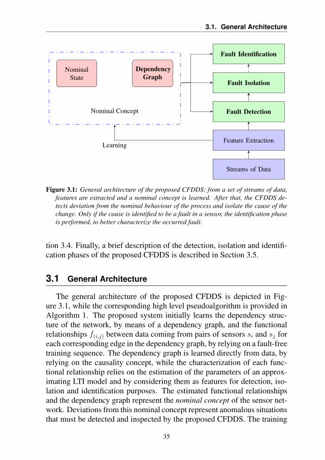
Streams of Data
Feature Extraction
Fault Detection
Fault Isolation
Fault Identification
Nominal Concept
DependencyGraph
NominalState
Learning
Figure 3.1: General architecture of the proposed CFDDS: from a set of streams of data,features are extracted and a nominal concept is learned. After that, the CFDDS de-tects deviation from the nominal behaviour of the process and isolate the cause of thechange. Only if the cause is identified to be a fault in a sensor, the identification phaseis performed, to better characterize the occurred fault.
tion 3.4. Finally, a brief description of the detection, isolation and identifi-cation phases of the proposed CFDDS is described in Section 3.5.
3.1 General Architecture
The general architecture of the proposed CFDDS is depicted in Fig-ure 3.1, while the corresponding high level pseudoalgorithm is provided inAlgorithm 1. The proposed system initially learns the dependency struc-ture of the network, by means of a dependency graph, and the functionalrelationships f(i,j) between data coming from pairs of sensors si and sj foreach corresponding edge in the dependency graph, by relying on a fault-freetraining sequence. The dependency graph is learned directly from data, byrelying on the causality concept, while the characterization of each func-tional relationship relies on the estimation of the parameters of an approx-imating LTI model and by considering them as features for detection, iso-lation and identification purposes. The estimated functional relationshipsand the dependency graph represent the nominal concept of the sensor net-work. Deviations from this nominal concept represent anomalous situationsthat must be detected and inspected by the proposed CFDDS. The training
35
Chapter 3. The Proposed Cognitive Fault Detection and Diagnosis System
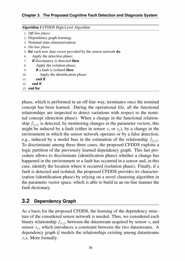
Algorithm 1 CFDDS High Level Algorithm
1: Off-line phase2: Dependency graph learning;3: Nominal state characterization;4: On-line phase5: for each new data vector provided by the sensor network do6: Apply the detection phase;7: if discrepancy is detected then8: Apply the isolation phase;9: if a fault is isolated then
10: Apply the identification phase;11: end if12: end if13: end for
phase, which is performed in an off-line way, terminates once the nominalconcept has been learned. During the operational life, all the functionalrelationships are inspected to detect variations with respect to the nomi-nal concept (detection phase). When a change in the functional relation-ship f(i,j) is detected, by monitoring changes in the parameter vectors, thismight be induced by a fault (either in sensor si or sj), by a change in theenvironment in which the sensor network operates or by a false detection,e.g., induced by a model bias in the estimation of the relationship f(i,j).To discriminate among these three cases, the proposed CFDDS exploits alogic partition of the previously learned dependency graph. This last pro-cedure allows to discriminate (identification phase) whether a change hashappened in the environment or a fault has occurred in a sensor and, in thiscase, identify the location where it occurred (isolation phase). Finally, if afault is detected and isolated, the proposed CFDDS provides its character-ization (identification phase) by relying on a novel clustering algorithm inthe parameter vector space, which is able to build in an on-line manner thefault dictionary.
3.2 Dependency Graph
As a basis for the proposed CFDDS, the learning of the dependency struc-ture of the considered sensor network is needed. Thus, we considered eachbinary relationship f(i,j) between the datastream acquired by sensor si andsensor sj , which introduces a constraint between the two datastreams. Adependency graph G models the relationships existing among datastreamsxis. More formally:
36

3.2. Dependency Graph
Definition 3.2.1. Given a sensor network S, a dependency graph G over Sis defined as:
G = (V,E), (3.1)
where V = s1, . . . , sn is the set of network sensors and E is a setof directed edges connecting sensors, such that the directed edge eij =(sj, si), eij ∈ E represents the relationship f(i,j) between datastreams xiand xj , provided by si and sj , respectively.
s1 s2
s3
s4s5s6
f(2,1)
f(3,1)
f(3,2)
f(4,1)f(4,2)
f(4,3)
f(5,1)
f(5,3)
f(6,1)
f(6,2)f(6,3)
Figure 3.2: Example of dependency graph for a network with n = 6 sensors. V =s1, . . . , s6 and E = e21, e31, e32, e41, e42, e43, e51, e53, e61, e62, e63. For eacheij ∈ E there is a non-trivial functional relationship f(i,j) between data measured bysensors si and sj .
An example of a dependency graph for a sensor network is shown inFigure 3.2. In the figure, it is possible to see that the sensor s1 has functionalrelationships with all the other ones, thus the values assumed by s2, . . . , s6
at a given time instant t influence the value acquired by sensor s1 at timet+ 1. The same does not apply to sensor s5, which is not influenced by anyother sensor, but it influences s1 and s3, i.e., functional relationships f(5,1)
and f(5,3) exist. Finally, for instance, the functional relationship f(5,4) is notincluded in G, since it does not exist or is too weak. In fact, the variationof the value measured by the sensor s5 does not influence the one in s4 andvice versa.
We would like to point out that the dependency graph G does not coin-cide with the network topology, but might be influenced by it. In fact, itis more likely that two sensors near each other have a stronger functionaldependency than far sensors. Nonetheless, depending on the specific appli-cation also distant sensors could be related as well, for instance the oceantemperature of water in the Mexican gulf influences the one on the coasts
37

Chapter 3. The Proposed Cognitive Fault Detection and Diagnosis System
of Northern Europe due to the Gulf Stream, thus a strong functional rela-tionship exists, even though those locations are topologically distant.
3.3 Modeling Functional Relationships Between Pairs of Sen-sors
Given the dependency graph of the sensor network G, a modeling tech-nique to analyse each single relationship between a couple of sensors f(i,j)
is needed. We emphasize that the theoretical results presented here are alsovalid for the case of a generic Multiple Input Single Output (MISO) func-tional relationship.
In the following, a functional relationship f(i,j) between the datastreamprovided by sensors si and sj is approximated through a LTI predictivemodel belonging to a familyM parametrised in θ ∈ DM, DM ⊂ Rp be-ing a compact C1 manifold. MISO linear predictive models [60], ExtremeLearning Machines (ELMs) [42], Reservoir Networks (RNs) [47, 74] arevaluable instances for M. A complete characterization of the propertiesneeded for the considered space is provided in the sequel. In this disserta-tion we opt to present the modeling methodology as a generic linear one-step-ahead predictive model in the form:
xj(t|θ) = f(i,j) (t, θ, xj(t− 1), . . . , xj(t− τj), xi(t), . . . , xi(t− τi + 1)) ,(3.2)
where f(i,j) : N × Rp × Rτj × Rτi → R is the approximating functionin predictive form [59], e.g., Auto Regressive eXogenous (ARX), AutoRegressive Moving Average eXogenous (ARMAX) model, t ∈ N is theconsidered time instant, xi(t), xj(t) ∈ R are the model input and output attime t, respectively, and τi and τj are the orders of the input and output,respectively. Given a training sequence (xi(t), xj(t))Nt=1 of length N anda quadratic loss function, we define the structural risk [59] to be:
WN(θ) =1
N
N∑t=1
E(xi,xj)
[ε2(t, θ)
], (3.3)
where E(xi,xj)[·] is the expected value over the space of the datastreams xiand xj of length N , and the empirical risk as:
VN(θ) =1
N
N∑t=1
ε2(t, θ), (3.4)
38

3.3. Modeling Functional Relationships Between Pairs of Sensors
where ε(t, θ) = xj(t)− xj(t|θ) is the prediction error at time t. The optimalparameter θo ∈ DM is defined as
θo = arg minθ∈DM
[lim
N→+∞WN(θ)
]. (3.5)
An estimate θ ∈ DM of θo can be obtained by minimizing the empiricalrisk:
θ = arg minθ∈DM
VN(θ). (3.6)
It has been showed that the parameter vector θ is characterized by a spe-cific asymptotic distribution. More formally, the following theorem holds:
Theorem 3.3.1 (Ljung [58, 59]). Consider a process P , a model spaceMparametrized by θ ∈ D(M), where D(M) is a compact C1 differentiablemanifold in Rp, a function l(·, ·, ·) : N × Rp × R → R+ and a structuralrisk function WN . Under the hypotheses that:
1. ∃C ∈ R+,∃λ ∈ R+, λ ≤ 1,∃δ ∈ R+, δ > 0 s.t. ∀t, ∀s s.t. t ≥s,∃x0
is(t),∃x0js(t) random vectors generated by [xi(0), . . . , xi(t)] and
[xj(0), . . . , xj(t)] respectively, independent from [xi(0), . . . , xi(s)] and[xj(0), . . . , xj(s)] s.t.:
E(xi,xj)
[|xj(t)− x0
js(t)|4+δ]< Cλt−s (3.7)
E(xi,xj)
[||xi(t)− x0
is(t)||4+δ]< Cλt−s (3.8)
where ||·|| is an appropriately defined norm and u0t (t) = 0, y0
t (t) = 0;
2. ∃C ∈ R, ∃λ ∈ R+, λ ≤ 1, ∀θ ∈ DM (thus ∀f ∈M)
|f(θ, xti1, xt−1j1 )− f(θ, xti2, x
t−1j2 )| (3.9)
≤ C
t∑s=0
λt−s [||xi1(s)− xi2(s)||+ |xj1(s)− xj2(s)|] ,
|f(θ, 0t, 0t−1)| ≤ C, (3.10)
where xt = (x(1), . . . , x(t) is a sequence drawn from the datastreamdistribution, || · || is a properly defined norm and 0t = (0, . . . , 0), i.e.,a particular Lipschitz continuity condition [76] suited for the spacewe are considering;
3. ∀f(θ, ·) ∈ M(θ), f(θ, ·) is three times differentiable w.r.t. θ ∈ DMand these derivatives satisfy the conditions of Point 2;
39

Chapter 3. The Proposed Cognitive Fault Detection and Diagnosis System
4. ∃C ∈ R+,∀θ ∈ DM, ∀t ∈ N s.t.:∥∥∥∥ ∂k∂θk l(t, θ, ε)∥∥∥∥ ≤ C||ε||2 k = 1, 2, 3 (3.11)∥∥∥∥ ∂k∂θk ∂∂εl(t, θ, ε)∥∥∥∥ ≤ C||ε|| k = 0, 1, 2 (3.12)∥∥∥∥ ∂k∂θk ∂2
∂ε2l(t, θ, ε)
∥∥∥∥ ≤ C k = 0, 1 (3.13)∥∥∥∥ ∂3
∂ε3l(t, θ, ε)
∥∥∥∥ ≤ C (3.14)
where || · || is a properly defined matrix norm;
5. ∃δ ∈ R+, ∃N0 ∈ R+ s.t. ∀θ ∈ DM, N ≥ N0:
W ′′N(θ) > δIp, (3.15)
where W ′′N is the Hessian matrix of the structural risk
WN(θ) =1
N
N∑t=1
E(xi,xj) [l(t, θ, ε(t, θ))] (3.16)
w.r.t. θ and Ip is the identity matrix of order p;
6. ∃δ ∈ R+ s.t. ΣN > δIp, UN > δIp where ΣN ∈ Rp×p is defined asfollows:
ΣN = [W ′′N(θo)]
−1UN [W ′′
N(θo)]−1, (3.17)
where UN ∈ Rp×p:
UN = NE(xi,xj)
[V ′N(θo)V ′N(θo)T
](3.18)
where it is required that the matrix ΣN is semidefinite positive, in or-der to be a proper covariance matrix;
then an estimated parameter vector θ estimated by minimizing the empiricalrisk:
VN(θ) =1
N
N∑t=1
l(t, θ, ε(t, θ)), (3.19)
on a sequence (xi(t), xj(t))Nt=1 satisfies
limN→∞
θ → θo w.p. 1 (3.20)
40

3.3. Modeling Functional Relationships Between Pairs of Sensors
and
limN→∞
√NΣ
− 12
N (θ − θo) ∼ N (0, Ip). (3.21)
The above result assures that, given a sufficiently large dataset, com-posed by N samples, the estimated parameter vector θ follows a multivari-ate Gaussian distribution with mean θo and covariance matrix ΣN . Interest-ingly, the results presented above contemplate the situation where P /∈ Mi.e., a model bias ||M(θo)−P|| 6= 0 is present. This justifies the use of LTImodels even when the dynamic system under investigation is non-linear.According to Equation (3.21), estimated parameters θs follow a multivari-ate Gaussian distribution both approximating linear and nonlinear systems,provided that a sufficiently large dataset is available. We emphasize that, inwhat follows, we are not interested in providing a high approximation ac-curacy, since LTI models are not used for prediction purposes (where non-linearities in the system might induce a high prediction error) but for faultdiagnosis. Parameter vectors are the features to be used for fault diagnosisand, since a change in the probability density function of the parameter/fea-tures is associated with structural changes in the process generating the data(and non-linearity does not introduce structural changes), we can design aCFDDS that relies on an analysis in the parameter space.
Although the nonlinearity aspect is contemplated by the theory, we mightexperience numerical problems in correspondence with an ill conditionedHessian W ′′
N , e.g., following highly correlated inputs. However, we mustcomment that if W ′′
N degenerates in rank then, given the linearity assump-tion for the considered approximation model, we should simply removethe linear dependent variables. In the case we wish to keep them for the(small) innovation they provide, a Levenberg-Marquardt (LM) correctionW ′′N + δIp (δ being a small positive scalar) should be introduced to grant a
definite positive Hessian.Extension to scenarios where the data generating process P is described
by a finite set of non-overlapping processes P1, . . . ,Pψ is immediate,as long as one knows the states of the system. Clearly this extension re-quires to have a priori information about the data generating process, forinstance on the seasonality of the system inspected by the sensor network.Moreover, here we considered as model the MISO models, but an exten-sion to Multiple Input Multiple Output (MIMO) and Single Input MultipleOutput (SIMO) is trivial, e.g., by considering a set of the aforementionedfunctional relationships.
41
Chapter 3. The Proposed Cognitive Fault Detection and Diagnosis System
3.4 Feature in the Parameter Space
From the theoretical results delineated in Section 3.3 parameter vectors es-timated from fault-free data are distributed according to a Gaussian distri-bution, provided that N is large enough (even though the system is non-linear). According to Equation (3.21), the nominal state of a system canbe described by parameter vectors estimated from data coming from theprocess, thus sampled from the same Gaussian distribution (each sampledpoint is a model).
Given the process P and the sensor network providing the multivariatedatastream X , let us define ZN,t ∈ Rn×N as a finite sequence from timet−N + 1 to t extracted from X . More formally:
ZN,t := [X(t−N + 1), . . . ,X(t)] , (3.22)
where N ∈ N is the length of the sequence extracted from the datastreamand t ≥ N, t ∈ N is the time instant the sequence of data considered ends.Moreover, if we want to consider only data coming from a specific coupleof sensors (si, sj) we define Z(ij)
N,t ∈ R2×N as:
Z(ij)N,t =
[xi(t−N + 1) . . . xi(t)
xj(t−N + 1) . . . xj(t)
], (3.23)
i.e., the sequence of samples coming from sensors si and sj , starting fromtime t−N + 1 and ending at time t.
For each couple of sensors si and sj , the proposed CFDDS relies onan initial fault-free training sequence Z(ij)
M,M , i.e., the acquired samples ac-quired from time t = 1 up to t = M , to characterize the nominal stateof the process. For fault diagnosis purposes the training set Z(ij)
M,M is win-dowed into non-overlapping batches Z(ij)
N,t of length N , each of which isused to provide a parameter vector estimate θq, q = t
N. The outcome is the
sequence of L = MN
1, L ∈ R+ parameter vectors:
Θ(ij)L,M =
(θ
(ij)1 , . . . , θ
(ij)L
), (3.24)
where the parameter vector θ(ij)q is estimated by minimizing the empirical
risk on the dataset Z(ij)N,qN , as described in Section 3.3.
1Without loss of generality we assume M is a multiple of N
42

3.5. The Phases of the Proposed CFDDS
We also considered estimate parameter vectors computed on overlap-ping batches of the training set Z(ij)
M,M . The obtained sequence is:
Θ′(ij)L,M =
(θ(ij)q
)Lq=1
(3.25)
where L = M −N + 1 and the parameter vector θ(ij)q is estimated by min-
imizing the empirical risk on the dataset Z(ij)N,N+q−1. Without loss of gen-
erality, we assume a step of one sample between two overlapping batches;larger steps could be considered as well (e.g., to reduce the computationalcomplexity of the following computations).
The twofold method for the estimation of the parameter vectors is dueto the fact that the former one is able to provide a clear statistical char-acterization for the parameter vector sequence distribution, since they arei.i.d., which can be used during the identification phase, while the latterlacks of this characterization but provides a parameter vector for each sam-ple coming from the sensor network, which is more suited for the detectionphase, since it provides a more fine grained characterization of the processbehaviour.
3.5 The Phases of the Proposed CFDDS
In the sequel, details about the phases considered in the proposed CFDDSare provided. They corresponds to the blocks with bold names in Figure 3.1and will be treated in detail in Chapters 4 to 7.
3.5.1 Graph Learning
The proposed CFDDS makes use of the concept of Granger causality toinfer the existing causal dependencies among datastreams [15]. Thanksto a statistical test performed directly on the training set ZM,M , we areable to assess the causal dependencies between couples of datastreams. Ifthe presence of the functional dependency f(i,j) is assessed, i.e., if the testprovides enough statistical confidence for the considered causality, an edgeis considered in the edge set E of the dependency graph G = (V,E). Thegraph G is not able to provide any diagnostic information per se, but it isused in the following phases: the detection and identification phases areperformed only on functional relationships in E, while the isolation phaseis based on the logic partition of the dependency graph. The dependencygraph learning procedure is detailed in Chapter 4.
43
Chapter 3. The Proposed Cognitive Fault Detection and Diagnosis System
3.5.2 Detection
The detection phase is performed on all the binary functional relationshipspresent in the dependency graph G. Each functional relationship the nom-inal concept is characterized by the sequence of parameter vectors Θ′L,M ,estimated on overlapping batches of data coming from a fault-free train-ing sequence ZM,M . The statistical behaviour of the parameter vectors se-quence is modeled by means of an approach based on HMMs [72]. Byrelying on this characterization, it is possible to evaluate the statistical com-patibility of a sequence of newly estimated parameter vectors Θ′k,t at time tby computing the loglikelihoods. A detection happens when the loglikeli-hood of the HMM decreases below an automatically determined threshold.The detailed description of the proposed cognitive fault detection phase isprovided in Chapter 5.
3.5.3 Isolation
The isolation phase is performed by relying on the learned dependencygraph of the sensor network G. Once a change has been detected, a cogni-tive level, which exploits a logical partition of the dependency graph G, isactivated. This mechanism is able to distinguish among a fault, a changein the environment and the presence of model bias [8, 12]. When a faultaffects a sensor, the relationships that are connected to that sensor willperceive a change (by means of a loglikelihood decrease). When there ischange in the environment, all the relationships in E are affected. Finally,when there is model bias in the considered relationship, none of the otherrelationships in E perceives a change. Furthermore, if the change is asso-ciated with a fault, the isolation phase is also able to provide informationabout its location, in terms of the affected unit. We would like to point outthat, even during this phase, the characterization of the nominal concept ofthe inspected system relying on HMM learned during the detection phaseis considered, but for isolation purposes. The isolation logic is formalizedand described in Chapter 6.
3.5.4 Identification
Once the fault is detected and isolated, the proposed CFDDS algorithm isable to provide a characterization of the occurred fault [10, 11]. This phaseis performed by means of a novel evolving clustering algorithm. Duringthe training phase, a characterization of the nominal state of the systemis performed by means of a clustering of the parameter vectors sequenceΘL,M , which are estimated on non-overlapping batches of data coming
44

3.5. The Phases of the Proposed CFDDS
from ZM,M . The theoretical results presented above allow to specificallydesign statistics to check if newly estimated vectors belongs to the nominalstate, according to the asymptotic distribution of the parameter vectors inthe parameter space. As soon as the presence of a fault is assessed in theprevious phases (detection and isolation) of the proposed CFDDS, it is iden-tified by associating it to one of the clusters present in the fault dictionary.This dictionary, which is initially empty, is automatically populated duringthe operational life of the proposed CFDDS. A new cluster representing afault is created only if enough confidence on the existence of a new faultis gathered (i.e., by performing a Kolmogorov-Smirnov (KS) multivariatetest on the expected and empirical distributions). The clustering mechanismconsidered for the identification phase is described in Chapter 7.
45


CHAPTER4Dependency Graph Learning
Since the dependency graph is at the basis of the fault detection, isolationand identification phases of the proposed CFDDS, the ability to learn it cor-rectly is fundamental to guarantee the fault detection and diagnosis perfor-mance. In particular, the ability to correctly learn the dependency graph iscrucial, since it allows the proposed CFDDS to rely only on the relevant re-lationships (i.e., those relationships that really exist among streams of data).This allows the proposed CFDDS to increase its performance for two mainreasons. At first, if we keep not relevant relationships in the dependencygraph, false positives in detection might increase, since all relationshipsare inspected in parallel. Second, if a relationship providing informationis not included in the dependency graph, we cannot use it in the isolationand identification phases to distinguish between the occurrence of a fault, achange in the environment or a model bias.
In this section, we describe the dependency graph learning phase ofthe proposed CFDDS, which is based on a statistical framework based onGranger causality. We recall that the dependency graph G = (V,E) is as-sociated to the functional relationships existing among data and not to thetopology of the network. The aim of the dependency graph learning phase,described in Figure 4.1, is to automatically select those relationships pre-
47

Chapter 4. Dependency Graph Learning
ZM,M
Feature extraction
Fault Detection
Fault Isolation
Fault Identification
Nominal Concept
GrangerG = (V,E)
NominalState
Learning
Learning
Figure 4.1: Dependency graph learning phase of the proposed CFDDS: by relying on afault-free dataset ZM,M and the concept of Granger causality, we select only thoserelationships which are relevant to the fault detection and diagnosis phases.
senting causal dependency given a fault-free set of measurements ZM,M
coming from the sensor network and a predefined level of confidence αgregulating the probability of including not relevant relationships in E. Inparticular, in Section 4.1 we describe the technique for assessing the causaldependency of a single relationship, while in Section 4.2 we extend thislearning mechanism to the entire dependency graph G.
4.1 Modeling the Relationship Between a Couple of Datas-treams
The level of dependency between datastreams xi and xj associated withrelationship f(i,j) has been analysed also in other FDDSs. For instance,in [8] the figure of merit used to select functional relationships is the linearcorrelation index between two datastreams: when the peak of the crosscor-relation is above a suitably tuned threshold ρmin, the relationship is consid-ered to be relevant and worth to be included in E. The main drawbacks ofthe aforementioned approach are the lack of a clear characterization of theuser-defined threshold ρmin (it is difficult to set it at design time), the capa-bility to assess relationships only between couples of datastreams (a rela-tionship involving more than two datastreams cannot be evaluated throughcross-correlation) and the fact that results are heavily dependent on noise,
48
4.1. Modeling the Relationship Between a Couple of Datastreams
as pointed out in [72].In the proposed CFDDS the method chosen to model the dependency be-
tween two datastreams relies on causal dependency as defined by Grangerin [38]:
Definition 4.1.1 (Granger Causality). Consider a bivariate discrete-timestochastic vector (xi, xj). We say that xi is Granger causing xj if the pres-ence of xi allows for better prediction performance of xj at time t.
Interestingly, approaches based on the Granger causality has been suc-cessfully applied to different application fields like economic [4] and medi-cal applications (e.g., functional Magnetic Resonance Imaging (fMRI) data [32]and ElectroEncephaloGraphy (EEG) analyses [20, 41]). To the best of outknowledge, the Granger causality have never been considered before forfault detection/diagnosis purposes in the existing literature.
Definition 4.1.1 is quite general and relies on the comparison betweentwo different reconstruction abilities: with and without xi as additionalsource of information. In the sensor network scenario, a more specific def-inition of Granger causality can be considered [19]:
Definition 4.1.2 (Multivariate Conditioned Granger Causality). Considera multivariate discrete-time stochastic vector X , we say that xi ∈ X isGranger causing xj ∈ X, j 6= i, conditioned to X \ xi, xj, if we arebetter able to predict xj by using X instead of using X \ xi.
Starting from the last definition, it is possible to derive a statistical testable to assess the multivariate conditioned Granger causality between twodatastreams. To assess if xi Granger causes xj , we need to model the rela-tionship existing among all datastreams provided by the sensor network asa linear Vector AutoRegressive (VAR) model [18, 39]. More specifically,following the Definition 4.1.2, we want to assess the influence of xi in theprediction of xj . To achieve this goal we consider two different versions ofthe VAR model:M(j)
f (full model), i.e., the one that considers all the avail-able datastreams X to predict xj , andM(ij)
r (reduced model), i.e., the oneconsidering as predictors only X \ xi. More formally, the two predictivemodels assume forms:
M(j)f : xj(t) =
τ∑k=1
n∑h=1
ahjkxh(t− k), (4.1)
M(ij)r : xj(t) =
τ∑k=1
n∑h=1,h6=i
a′hjkxh(t− k), (4.2)
49

Chapter 4. Dependency Graph Learning
where ahjk ∈ R and a′hjk ∈ R are the regression coefficients modeling thelinear relationship between measurements coming from sensors sh and sjat the k-th time lag for modelM(j)
f andM(ij)r , respectively, and τ ∈ N is
the order of the model1.It is possible to show that the problem of assessing the multivariate con-
ditional Granger causality can be formulated as a loglikelihood ratio testbetween the full model M(j)
f and the reduced model M(ij)r [50], where
the null hypothesis is that xi is not Granger causing xj conditioned toX \ xi, xj. More specifically, given a training sequence ZM,M , we esti-mate parameters ahjk ∈ R and a′hjk ∈ R by mean of a LS procedure appliedto ZM,M . The loglikelihood ratio test is based on the computation of the teststatistic:
Fij =pf − pr
M − pf − 1
SSR(ij)r − SSR(j)
f
SSR(j)f
∼ F (pf − pr,M − pf − 1) (4.3)
where pf = nτ is the number of parameters of the full modelM(j)f , pr =
(n − 1)τ is the number of parameters of the reduced one M(ij)r , F (pf −
pr,M − pf − 1) is the Fisher distribution with pf − pr and M − pf − 1
degrees of freedom, SSR(j)f and SSR(ij)
r are the sum of squared residualon ZM,M of the modelM(j)
f andM(ij)r , respectively. In the test, the critical
region of level αg for the statistic is:
Rαgij = F ∈ R+|F ≥ Fαg(pf − pr,M − pf − 1), (4.4)
where Fαg(pf − pr,M − pf − 1) is the quantile of order 1 − αg of theFisher’s distribution with pf−pr andM−pf−1 degrees of freedom. Whenthere is statistical evidence for rejecting the null hypothesis with confidence1−αg (i.e., Fij ∈ Rαg
ij ), we say thatFxi→xj |z, i.e., the datastream xi Grangercauses xj conditioned to z = X\xi, xj, since the datastream xi improvesthe prediction of xj . Thus, αg represents the probability to infer that theuse of xi does not improve the prediction of xj when it actually does (typeI error): the more one chooses low values for αg, the more the chance thata relationship is included in the learned dependency graph when it does notexists in the real one decreases.
It is worth noting that, in principle, to evaluate the contribution in pre-diction abilities of datastream xi to stream xj , one could inspect the exoge-nous coefficients corresponding to xi in the full modelM(j)
f , i.e., aijk ∀k ∈1Albeit VAR models are linear models, it is possible to show that, under mild assumptions about the data-
generating process (e.g., stationarity of the covariance), they are general enough to model several nonlinearmultivariate time series [16].
50

4.2. Creating the Granger-based Dependency Graph
1, . . . , τ. When these coefficients are statistically null (meaning thatstream xi does not provide improvement in the prediction of stream xj),there is no causal dependency of datastreams xj from xi. On the contrary,when at least one of the coefficients differs from zero, a causal depen-dency relation between the two datastreams exists. Interestingly, it is shownin [50] that the problem of identifying a causal dependency between datas-treams xi and xj , formulated in Equation (4.4), is equivalent to a hypothesistest which assesses if at least one of the coefficients aijk, k ∈ 1, . . . , τ isstatistically different from zero, i.e.:
H0 : aijk = 0 ∀k vs. H1 ∃k | aijk 6= 0. (4.5)
4.2 Creating the Granger-based Dependency Graph
Following the definition of Granger causality and the statistical test de-scribed above, it is possible to derive a statistical framework to learn thedependency graph for the whole sensor network. A detailed description ofthe proposed statistical framework is provided in Algorithm 2.
Algorithm 2 Granger-Based Dependency Graph Learning Algorithm
1: Input: faulty-free dataset ZM,M , confidence level αg2: Output: dependency graph G3: Set an empty dependency graph G = (V,E), with V = s1, . . . sn and E = ∅4: for j ∈ 1, . . . , n do5: Estimate coefficients aijk of VAR modelM(j)
f in Equation (4.1) from data ZM,M ;6: for i ∈ 1, . . . , n do7: if i 6= j then8: Estimate coefficients a′ijk of VAR model M(ij)
r in Equation (4.2) from dataZM,M ;
9: Compute Fij as in Equation (4.3);10: if Fij ≥ F αg
n(n−1)(pf − pr,M − pf − 1) then
11: E ← E ∪ eij;12: end if13: end if14: end for15: end for16: return G;
At first, we consider a training set ZM,M of fault-free data coming fromthe sensor network and a user defined confidence level αg ∈ (0, 1) for theloglikelihood ratio test. A graph G = (V,E) with V = s1, . . . , sn andE = ∅ is initially considered. By considering a couple of sensors si and sj
51
Chapter 4. Dependency Graph Learning
and the dataset ZM,M , we are able to compute the test statistics Fij , as inEquation (4.3). When:
Fij ≥ F αgn(n−1)
(pf − pr,M − pf − 1), (4.6)
we have statistical evidence (with confidence αgn(n−1)
) that xi Granger causesxj , conditioned on all the other streams of data, and we add eij = (si, sj)to the edge set E. We repeat the test for each couple of datastreams tobuild the dependency graph. Note that we used a confidence level αg
n(n−1)to
obtain an overall confidence level of αg, thanks to the Bonferroni correctionfor multiple hypothesis [50]. The correction is here used since n(n − 1)hypothesis tests are performed at the same time and it assures to have anoverall type I error of αg.
We emphasize that both the performance and the complexity of the de-tection and isolation phases of the proposed CFDDS are highly influencedby the learned Granger-based dependency graph. In fact, the detectionphase will be performed on each edge eij ∈ E, while the isolation phaserelies on G to be able to distinguish among model bias, change in the envi-ronment and fault and, if this third option occurs, isolate it.
An example of the dependency graph learning phase is presented in Fig-ure 4.2. To determine the dependency graph, a fault-free dataset ZM,M isrequired. Starting from an completely disconnected graph (in the upperright part of the figure), the Granger-based statistical test considered is ableto determine which are the most relevant functional relationships existingamong datastreams. The confidence on the overall procedure is given bysetting αg.
52
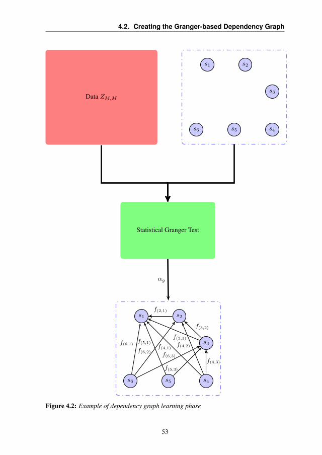
4.2. Creating the Granger-based Dependency Graph
s1 s2
s3
s4s5s6
Data ZM,M
Statistical Granger Test
s2s1
s3
s4s5s6
f(2,1)
f(3,1)
f(3,2)
f(4,1)f(4,2)
f(4,3)
f(5,1)
f(5,3)
f(6,1)
f(6,2)f(6,3)
αg
Figure 4.2: Example of dependency graph learning phase
53

CHAPTER5Fault Detection
In this chapter, we want to inspect the variation of the behaviour in therelationships f(i,j) such that eij ∈ E to understand if a deviation from thenominal concept occurred (detection phase). We suppose to have learneda dependency graph G = (V,E), which describes the causal relationshipsexisting among datastreams, as described in Chapter 4. In order to detectchanges in the behaviour of the data coming from the sensor network, weconsider all the binary relationships f(i,j) in parallel. Here we want to learna characterization of each functional relationship in nominal conditions andbe able to detect discrepancies from it.
In this chapter the detection phase of the proposed CFDDS is provided:at first, the general approach in the parameter space is delineated in Sec-tion 5.1, then the description of a Mahalanobis-based change detectionmethod is presented in Section 5.2. A description of HMM-CDT, intro-duced in [7] and further developed in [72], is given in Section 5.3, whilethe proposed Ensemble approach to Hidden Markov Model-Change Detec-tion Test (EHMM-CDT) is detailed in Section 5.4.
55

Chapter 5. Fault Detection
Process Sensors Y
ε (Noise)
LTI Model
Parametersθ
ChangeDetection
NominalbehaviourZM,M
Change Fault
Figure 5.1: Proposed scheme for fault detection: we do not have a priori information onthe process, the sensors or the noise ε.
5.1 Fault Detection in the Parameter Space
The detection phase of the proposed CFDDS is based on the analysis of thestatistical behaviour the estimated parameter vectors presented in Chap-ter 2. Let us consider a generic functional relationship between a coupleof streams f(i,j) s.t. eij ∈ E. By relying on a fault-free training datasetZ
(i,j)M,M , it is possible to compute a parameter vectors sequence Θ
(ij)L,M or
Θ′(ij)L,M , which characterizes the nominal conditions of the system. After
that, we want to inspect newly estimated parameter vectors of the functionalrelationships f(i,j) selected during the graph learning phase and detect vari-ations in their behaviour.
The general approach considered in this dissertation is presented in Fig-ure 5.1. Since in the sensor network scenario the generating data pro-cess is unknown, as well as the noise characterization, we can not rely ontraditional approaches (signal-based or model-based, as described in Sec-tion 1.1.1). The approach considered in the proposed CFDDS relies onthe approximation the relationship existing among datastreams with a LTImodel, which is able to capture the functional relationship f(i,j) deviation
56

5.2. Mahalanobis-based Detection
Z(ij)M,M
Θ(ij)L,M
Region Rαs
Fault Isolation
Fault Identification
Nominal Concept
DependencyGraph
Distribution(θ,SN )
Learning
Figure 5.2: Mahalanobis-based detection phase of the proposed CFDDS: by relying on afault-free dataset Z(ij)
M,M , the parameter vector sequence Θ(ij)L,M is extracted. They are
used to learn the nominal state by means of a Gaussian distribution in the parameterspace and a region Rαs for the parameter vectors not belonging to the nominal state.
from nominal behaviour. By considering as feature for fault detection thevariations of the LTI estimated parameters θs, we are able to detect changesin the behaviour of the data from the one we recorded in nominal condi-tions. The discrepancy from the nominal behaviour can be assessed only ifa correct characterization of the nominal concept is performed beforehand:here we perform a characterization in the parameter space by relying ona fault-free dataset ZM,M . Two different methods based on this paradigmare presented in the following: the former one exploits the asymptotic dis-tribution of the parameters, while the latter one is able to characterize thesequence of the parameter vectors through a HMM modeling approach.
5.2 Mahalanobis-based Detection
Thanks to Equation (3.21), the parameter vectors in Θ(ij)L,M are distributed
as a multivariate Gaussian distribution, which is fully characterized by itsmean θo and covariance matrix ΣN . Thus, in the parameter space it is pos-sible to define a region where with probability 1−αs the parameter vectorsestimated from data coming from nominal state can be drawn, by relyingon the Mahalanobis distance [63]. This approach has been considered inthe past, for instance, for quality control charts [50].
57

Chapter 5. Fault Detection
Algorithm 3 Mahalanobis-Based Change Detection Algorithm
1: Data: Training set Z(ij)M,M , Confidence level αs;
2: Results: Detection time T ;3: Estimate the sequence Θ
(ij)L,M from Z
(ij)M,M ;
4: Compute θ and SN ;5: while a new parameter vector θ(ij)
t is available at time t do6: if θt /∈ Rαs then7: return T ← t;8: end if9: end while
10: return T ← ∅;
The general architecture of the detection phase based on this distance ispresented in Figure 5.2 and an algorithm describing the procedure to applythe Mahalanobis-based detection method is provided in Algorithm 3. Themean θ ∈ Rp and covariance SN ∈ Rp×p can be estimated by using Θ
(ij)L,M
and constitute the definition of nominal cluster used in the sequel of thedissertation. More formally:
Definition 5.2.1. Given a parameter vectors sequence Θ(ij)L,M estimated on
a dataset Z(i,j)M,M coming from a single process P , a Gaussian cluster Υ,
induced by the sequence Θ(ij)L,M , is a tuple (θ, SN , υ) (υ ∈ N), where:
θ =1
υ
∑θ∈Θ
(ij)L,M
θ, (5.1)
SN =1
υ − 1
∑θ∈Θ
(ij)L,M
(θ − θ)(θ − θ)T , (5.2)
υ = |Θ(ij)L,M |, (5.3)
and | · | is the cardinality operator.
A Gaussian cluster induces a topology on the parameter space, identifiedby the Mahalanobis distance [63], defined as:
Definition 5.2.2. Given a parameter vector θ(ij)t ∈ Rp and a Gaussian
cluster Υ = (θ, SN , υ), the Mahalanobis distance m(θ(ij)t ,Υ) between the
vector θ(ij)t and the cluster Υ is defined as:
m(θ(ij)t ,Υ) = (θ − θ(ij)
t )TS−1N (θ − θ(ij)
t ). (5.4)
58

5.2. Mahalanobis-based Detection
θ1
θ2
αs = 0.05
Figure 5.3: Example of Mahalanobis-based detection in 2 dimension (θ1, θ2): the param-eter vectors estimated on the training set (black circles) defines the nominal state; anarea of probability 1 − αs = 0.95 is defined by the ellipse. The detection phase isable to discriminate between points belonging to the nominal state region Rαs (greenasterisks) and those not belonging to it (red pluses), with confidence 1− αs.
Since theoretical results presented in Section 3.3 allow us to assume theGaussian distribution of the estimated parameter vectors, a neighbourhoodcentered in θ can be induced by containing those θ(ij)
t s belonging to thenominal state with probability 1− αs [50], where αs is a given confidencelevel. More specifically, the neighbourhoodRαs , containing parameter vec-tors which belong to the nominal cluster, is defined as:
Rαs =
θ | υ(υ − p)
p(υ2 − 1)m(θ,Υ) ≤ Fαs(p, υ − p)
, (5.5)
where Fαs(p, υ−p) is the quantile of order 1−αs of the Fisher’s distributionwith parameters p and υ − p.
For instance, in Figure 5.3, an example of the detection phase in a twodimensional parameter vector space θ = (θ1, θ2) is provided. The nom-inal state is characterized by the black circles, estimated on the trainingset Z(i,j)
M,M : the knowledge of the statistical distribution allows us to definea region Rαs where a newly estimated parameter vector should fall withprobability 1−αs = 0.95 (inside the black ellipse). New parameter vectorsare considered belonging to the nominal state if they fall inside the ellipse
59

Chapter 5. Fault Detection
S1
S2
S3
θ ∼ D(S1)
θ ∼ D(S2)
θ ∼ D(S3)
a11
a12
a13
a21
a22
a23a31
a32
a33
Figure 5.4: Example of HMM: it has three hidden states S1, S2, S3 with transition matrixA = [aij ] and each states Si has emission θ, distributed as D(Si).
(green asterisks), while a change is detected when a parameter vector fallsoutside Rαs (red pluses).
The proposed Mahalanobis-based detection is potentially a powerful andversatile method for detection, since it relies on a grounded theoretical baseand requires only to set a confidence value αs (which has a specific sta-tistical meaning). Nonetheless, it is potentially a slow method, since themethod operates on non overlapping windows and a detection could hap-pen only every N time instants. In the following we rely on a differentmodeling of the nominal concept based on the estimation of parameter vec-tors on overlapping batches, i.e., by estimating Θ
′(ij)L,M on Z(i,j)
M,M instead ofΘ
(ij)L,M , to reduce the detection delay of this approach. Another drawback of
the aforementioned method is that it provides a structural amount of falsepositive detections over time. In fact, the use of a statistical test impliesto have the probability of αs structural false positives (type I error) at eachtime instant. By repeating the test multiple time in an on-line manner, thisprobability increases, for instance, after k time instant the methods has theprobability of a false positive detection of 1 − (1 − αs)k, whose limit fork →∞ is 1.
60

5.3. Hidden Markov Model Change Detection Test
Z(ij)M,M
Θ′(ij)L,M
HMM-CDT
Fault Isolation
Fault Identification
Nominal Concept
DependencyGraphHMM H
Learning
Figure 5.5: HMM-CDT detection phase: by relying on a fault-free dataset Z(ij)M,M , the
parameter vectors sequence Θ′(ij)L,M is extracted. It is used to learn the nominal state by
means of a HMM, which is used for discrepancy detection in the proposed HMM-CDT.
5.3 Hidden Markov Model Change Detection Test
The idea underlying the HMM-CDT is to analyse the statistical behaviourof the sequence of parameter vectors Θ
′(ij)L,t , estimated from X , over time
by means of a HMM modeling. A HMM is a statistical Markov model, inwhich the system being modeled is assumed to be a Markov process whosestates are neither known, nor observed. An example of a HMM with threehidden states (S1, S2, S3) is presented in Figure 5.4. While in traditionalMarkov chains, the state is observed and therefore the state transition prob-abilities aij are the only parameters to be estimated, in a HMM each state Siis not directly visible, but only the output θ, emitted from one of the stateswith a given distributionD(Si), is visible. Therefore, a sequence of outputsgenerated by a HMM provides information about the state sequence andcan be used to learn the HMM parameters, i.e., number of states, transitionmatrix and emitting distributions. HMMs have been successfully appliedto temporal pattern recognition problems such as speech recognition [70]and biology [55].
The HMM modeling approach applied to θ(ij)t s allow us to continuously
inspect the relationship behaviour: when the statistical pattern of the esti-mated parameters does not follow what was learned during an initial train-
61

Chapter 5. Fault Detection
ing phase, a change in the relationship is detected. The general scheme ofthe HMM-based detection phase is presented in Figure 5.5. The use of aHMM ruled by a Gaussian Mixture Model (GMM) over a parameter vectorssequence Θ
′(ij)L,t is the natural solution to model a functional relationship in
the parameter space, since it is capable of modeling a Gaussian distributionand even take care of the possible seasonality or periodicity effects presentin the data coming from a sensor network. More formally, a HMM [34] canbe defined as a tupleH = (S,A, π), where:
• S = S1, . . . , Ss, s ∈ N is the indexed set of the states, each of whichhas an emission distribution D(Si), defined by a GMM
• A ∈ Rs×s, A = [aij],∑s
i=1 aij = 1 ∀j ∈ 1, . . . , s is the transitionmatrix, i.e., aij is the transition probability from state i to state j;
• π ∈ [0, 1]s, with∑s
i=1 πi = 1, is the initial distribution probabilityover S.
Algorithm 4 HMM-CDT Algorithm
1: Data: Training set Z(ij)M,M , Validation set Z(ij)
O,M+O, CD;2: Results: Detection time T ;3: Estimate the sequence Θ
′(ij)L,M from Z
(ij)M,M ;
4: Estimate HMM H by using Θ′(ij)L,M ;
5: Estimate the sequence Θ′(ij)O,O+M from Z
(ij)O,M+O;
6: for h ∈ M + k, . . . , O do7: Compute l(H,Θ′(ij)k,h ) as in Equation (5.6);8: end for9: Compute T as in Equation (5.7)
10: while a new sample [xi(t), xj(t)] is available at time t do11: Estimate θ(ij)
t by using Z(ij)N,t ;
12: Built the sequence Θ′(ij)k,t = (θ
(ij)t−k+1, . . . , θ
(ij)t );
13: Compute l(H,Θ′(ij)k,t ) as in Equation (5.6);
14: if l(H,Θ′(ij)k,t ) ≤ T then15: return T ← t;16: end if17: end while18: return T ← ∅;
The HMM-CDT method is described in Algorithm 4. The HMM-CDTrelies on an initial parameter vector sequence Θ
′(ij)L,M , estimated on over-
lapping batches of N data extracted from the fault-free training set Z(i,j)M,M ,
62

5.3. Hidden Markov Model Change Detection Test
where L = M − N + 1. The parameter sequence Θ′(ij)L,M is used to train
a HMM H, aiming at capturing the statistical behaviour of the estimatedparameter vectors sequence Θ
′(ij)L,M in nominal conditions. Then, during the
operational phase, the statistical affinity between the estimated parametervectors θ(ij)
t and H is assessed by looking at the HMM loglikelihood asfollows:
Definition 5.3.1. Given a parameter vector sequence Θ′(ij)k,t = (θ
(ij)t−k+1, . . . , θ
(ij)t )
and a HMM H the loglikelihood is defined as:
l(H,Θ′(ij)k,t ) = log Pr(θ(ij)t−k+1|H) +
t−1∑h=t−k+1
log Pr(θ(ij)h+1|H, θ
(ij)h ). (5.6)
where Pr(A|H, B) is the probability associated to the parameter vectorA given as model the HMM H and the previously seen parameter vectorsspecified in B.
The loglikelihood provides an estimate on how well the sequence Θ′(ij)k,t
follows H, thus it can be used to detect changes in the relationship char-acterizing the nominal state of the system. In fact, if the relationship doesnot change over time, the value of the loglikelihood l(H,Θ′(ij)k,t ) is compa-rable with the one computed during the training phase. Otherwise, in casel(H,Θ′(ij)k,t ) falls below an automatically defined threshold T , a change isdetected, since Θ
′(ij)k,t is no more compatible with the statistical model char-
acterized by H. More specifically, by relying on a validation set Z(ij)O,M+O,
we compute a threshold T :
T = l − CD[l − min
h∈M+k,...,Ol(H,Θ′(ij)k,h )
](5.7)
where
l =
∑Oh=M+k l(H,Θ
′(ij)k,h )
O(5.8)
and CD > 1 is a user-defined coefficient factor, regulating the trade-off be-tween the false positive detection rate and the promptness in the detectionachieved by the HMM-CDT. High values for the parameterCD correspondsto low false positive rate and an high delay in the time of detection, whilelow values provide a prompter detection but an higher amount of false pos-itive detections.
63
Chapter 5. Fault Detection
During the operational life of the system, when the loglikelihood de-creases below T , a change in the statical behaviour of P is detected by theHMM-CDT. In more details, as soon as a new sample [xi(t), xj(t)] , t >
M + O is available, the algorithm estimates a new parameter vector θ(ij)t
on Z(ij)t,N . The likelihood for the HMM characterizing the nominal state, i.e.,
l(H,Θ′(ij)k,h ), is computed and is compared with the threshold T to assess if achange is detected. In case of a change, an alarm is raised and the detectiontime T = t is returned, otherwise the algorithm keeps on monitoring datacoming from the inspected process P .
5.4 Ensemble Approach to HMM-CDT
One of the key aspects of the HMM-CDT presented above is the estimationof a HMM on Θ
′(ij)L,M , which aims at properly characterizing the nominal
state. The state-of-the art training algorithm for HMMs is the Baum-Welch(BW) algorithm [22], which aims at finding the maximum likelihood esti-mates of the HMM parameters, given Θ
′(ij)L,M . Nonetheless, the BW algo-
rithm does not provide any theoretical guarantee about the convergence tothe global maximum of the likelihood function [31]. In fact, the BW al-gorithm requires a random initialization of the HMM parameters for theoptimization procedure, which could lead the algorithm to get stuck to alocal maximum. Thus, different estimated parameters for the HMM can beobtained by repeating the training phase with different randomly initializedparameters on the same training sequence Z(i,j)
M,M . Hence, a viable solutionto weaken the effect of the initialization procedure on the HMM-CDT isto repeat the use of BW algorithm and select the HMM guaranteeing thelargest likelihood on a validation set. Unfortunately, as pointed out in [62],this solution may lead to overfit the training sequence Θ
′(ij)L,M (and this is
particularly evident for reduced training sets), leading to false positive de-tections (false alarms) during the operational life of the system.
In the framework of the proposed CFDDS, we extend the solution pro-posed in Section 5.3 by suggesting an Ensemble approach to Hidden MarkovModel-Change Detection Test (EHMM-CDT) based on a set E = H1, . . . ,HQ,Q ∈ N of HMMs, where Q is the ensemble cardinality. Interestingly, thepossibility to combine different models to improve the generalization abil-ity of a single model has been widely studied in the literature (mainly in theregression and classification scenarios) and effectively applied to differentapplication fields [54, 68, 91]. Recently, ensembles of models have beenalso successfully considered in time series prediction [82, 89] and on-line
64

5.4. Ensemble Approach to HMM-CDT
Z(ij)M,M
Θ′(ij)L,M
EHMM-CDT
Fault Isolation
Fault Identification
Nominal Concept
DependencyGraph
ensembleof HMM E
Learning
Figure 5.6: Detection phase of the proposed CFDDS: by relying on a fault-free datasetZ
(ij)M,M , the parameter vector sequence Θ
′(ij)L,M is extracted. It is used to learn the nomi-
nal state by means of an ensemble of HMM, which are used for discrepancy detectionin the proposed EHMM-CDT.
missing data reconstruction [9]. Moreover, an ensemble of HMMs withina Bayesian framework for parameter estimation has been derived in [62],while an algorithm for training HMMs in the ensemble framework is pre-sented in [29].
The general scheme of the proposed detection phase is described in Fig-ure 5.6. The main point of the proposed solution is that the HMMsHq ∈ Eare trained on the same training set Z(ij)
M,M with different initialization pointsof the BW algorithm. This ensemble approach allows to weaken the influ-ence of the initial conditions of the HMM training algorithm, providinga better generalization ability and, consequently, better detection perfor-mance.
The proposed EHMM-CDT is detailed in Algorithm 5. To characterizethe nominal state we rely on a training set Z(ij)
M,M , which is assumed to bechange-free. We estimate the parameter vectors sequence Θ
′(ij)L,M on overlap-
ping windows of N data Z(ij)N,t . We build the ensemble E = H1, . . . ,HQ
by repeating e times the training of a HMM on Θ′(i,j)L,M , with random initial
conditions for the BW algorithm. Note that, since Z(ij)M,M is assumed to be
change-free, the ensemble E aims at modeling the statical behaviour of P
65

Chapter 5. Fault Detection
Algorithm 5 EHMM-CDT algorithm
1: Data: Training set Z(ij)M,M , Validation set Z(ij)
O,M+O, Aggregation method A, CD;2: Results: Detection time T ;3: Estimate the sequence Θ
′(i,j)L,M from Z
(ij)M,M ;
4: for q ∈ 1, . . . , Q do5: Estimate HMMHq using Θ
′(i,j)L,M by considering a random initialization point;
6: end for7: Built the ensemble E = H1, . . . ,HQ;8: Estimate the sequence Θ
′(i,j)M,M+O from Z
(ij)O,M+O;
9: for h ∈ M + k, . . . , O do10: for q ∈ 1, . . . , Q do11: Compute l(Hq,Θ′(i,j)k,h ) as in Equation (5.6);12: end for13: Compute A(h) = A(l(H1,Θ
′(i,j)k,h ), . . . , l(HQ,Θ′(i,j)k,h ));
14: end for15: Compute T as in Equation (5.11);16: while a new couple [xi(t), xj(t)] is available at time t do17: Estimate θ(i,j)
t by using Z(ij)N,t ;
18: Built the sequence Θ′(i,j)k,t ;
19: for q ∈ 1, . . . , Q do20: Compute l(Hq,Θ′(i,j)k,t ) as in Equation (5.6);21: end for22: Compute A(t) = A(l(H1,Θ
′(i,j)k,t ), . . . , l(HQ,Θ′(i,j)k,t ));
23: if A(t) ≤ T then24: return T ← t;25: end if26: end while27: return T ← ∅;
in nominal conditions.
One of the key aspects of ensemble methods is the definition of the ag-gregation mechanism A, that, in this case, specifies how to aggregate theloglikelihoods of the ensemble elements Hq ∈ E to provide the ensembleoutput. In this dissertation, we considered two different aggregation mech-
66

5.4. Ensemble Approach to HMM-CDT
anisms, i.e., A ∈ Amean,Amin:
A(t) = Amean(l(H1,Θ′(i,j)k,t ), . . . , l(HQ,Θ
′(i,j)k,t ))) =
Q∑q=1
l(Hq,Θ′(i,j)k,t )
Q
(5.9)
A(t) = Amin(l(H1,Θ′(i,j)k,t ), . . . , l(HQ,Θ
′(i,j)k,t ))) = min
q∈1,...,Ql(Hq,Θ
′(i,j)k,t ),
(5.10)
whereAmean computes the average value of the loglikelihoods of the HMMsbelonging to the ensemble E , whileAmin takes into account their minimum.The last step of the EHMM-CDT training phase is the computation of thethreshold T on a validation set Z(ij)
O,O+M . Similarly to what presented inSection 5.3, T is computed as follows:
T = l − CD[l − min
h∈M+k,...,OA(h)
](5.11)
where l =∑Oh=M+k A(h)
O.
An example of the proposed approach with Q = 5 is proposed in Fig-ure 5.7. At first the characterization of the process nominal conditions is ob-tained through the estimation of the ensemble of HMMs E = H1, . . . ,H5,trained on the same couple of datastreams (xi, xj). Each HMM providesa value for the loglikelihood on newly samples coming from the streams(xi, xj). Loglikelihood values are used in an aggregation mechanism A toassess if a change has occurred.
While ensemble approaches are generally able to increase the general-ization ability of a single model, they are characterized by an increasedcomputational complexity, that in this case scales linearly with the numberof HMMs Q. Two comments arise:
• the most time consuming part of the EHMM-CDT refers to the HMMstraining (the loglikelihood computation is much lighter than training).Interestingly, the training phase is performed only once during theinitial configuration of the proposed CFDDS, while during the oper-ational life only the likelihoods are computed. In addition, in sce-narios where networked embedded systems are operating, the train-ing of HMMs could be performed in a centralized high-powerful unit,leaving only the computation of likelihoods directly at the low-powerdistributed units of the network;
67

Chapter 5. Fault Detection
xi
xj
H1
H2
H3
H4
H5
A(H1, . . . ,H5) Detection result
l(H1)
l(H2)
l(H3)
l(H4)
l(H5)
Figure 5.7: Example of EHMM-CDT with Q = 5. The loglikelihood computed on eachelement of the ensemble of HMM l(Hq) provides information about the discrepancy ofthe process from nominal conditions. The detection decision occurs after the loglikeli-hoods are aggregated through a suitable aggregation mechanism A.
68

5.4. Ensemble Approach to HMM-CDT
• in scenarios where the fault detection ability is a relevant activity, theincrease in the complexity induced by the ensemble approach is wellcompensated if we are able to decrease false and missed alarms anddetection delays.
As a final remark we would like to point out that the extension of theproposed EHMM-CDT to multiple functional relationships is trivial (thedetection occurs when at least one change is detected in a functional rela-tionship). Moreover, its extension to MIMO models is possible, but is notsuggested here, since it does not allow to perform the isolation phase asproposed in Chapter 6.
69

CHAPTER6Fault Isolation
Once we are aware of the fact that the data provided by the sensor net-work are deviating from the nominal behaviour, by relying on the detectiontechnique presented in Chapter 5, the following step is to infer if this dis-crepancy is due to a change of the environment in which the network isoperating, to a fault in a specific sensor or to a model bias. To distinguishamong these situations we have to consider both the dependency graph Gand the HMM modeling used in the previous phases. The isolation phase ofthe proposed CFDDS, presented in Figure 6.1, is based on a logic partitionof the dependency graph edge set and the evaluation of the loglikelihoodprovided by the ensemble E on each of the partitions. In Section 6.1, wedescribe the overall cognitive isolation logic, while in Section 6.2 we de-scribe in detail the proposed isolation phase.
6.1 Cognitive Fault Isolation
We here consider the dependency graph G = (V,E) learned during the de-pendency graph learning phase (Chapter 4) and the result of the detectionprovided by the detection phase (Chapter 5), i.e., detection of a change ona specific functional relationship f(i,j). From now on, we assume that the
71
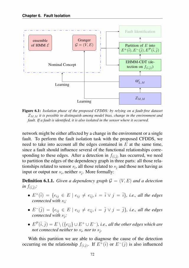
Chapter 6. Fault Isolation
ZM,M
Θ′L,M
EHMM-CDT (de-tection on f(i,j))
Partition of E intoE+(i), E−(j), EP (i, j)
Fault Identification
Nominal Concept
GrangerG = (V,E)
ensembleof HMM E
Learning
Learning
Figure 6.1: Isolation phase of the proposed CFDDS: by relying on a fault-free datasetZM,M it is possible to distinguish among model bias, change in the environment andfault. If a fault is identified, it is also isolated in the sensor where it occurred.
network might be either affected by a change in the environment or a singlefault. To perform the fault isolation task with the proposed CFDDS, weneed to take into account all the edges contained in E at the same time,since a fault should influence several of the functional relationships corre-sponding to these edges. After a detection in f(i,j) has occurred, we needto partition the edges of the dependency graph in three parts: all those rela-tionships related to sensor si, all those related to sj and those not having asinput or output nor si, neither sj . More formally:
Definition 6.1.1. Given a dependency graph G = (V,E) and a detectionin f(i,j):
• E+(i) = eij ∈ E | eij 6= eij, i = i ∨ j = i, i.e., all the edgesconnected with si;
• E−(j) = eij ∈ E | eij 6= eij, i = j ∨ j = j, i.e., all the edgesconnected with sj;
• EP (i, j) = E \ (eij ∪E+ ∪E−), i.e., all the other edges which arenot connected neither to si, nor to sj .
With this partition we are able to diagnose the cause of the detectionoccurring on the relationship f(i,j). If E+(i) or E−(j) is also influenced
72
6.1. Cognitive Fault Isolation
by the change, we may infer that a fault has happened on sensor si or sj ,respectively. In the case EP (i, j) is also influenced by the change, we arefacing a change in the environment inspected by the network, while if noother relationship is influenced by the detected change we infer that thecause is an incomplete characterization of the nominal state (model bias).
Finally, we define two properties of the fault affecting sensors includedin the dependency graph G. In fact, depending on its topology, a fault canbe isolated on a specific subset of nodes. Formally:
Definition 6.1.2. Given a dependency graph G = (V,E), a fault F oc-curring in the sensor sh ∈ V is detectable if and only if ∃eij ∈ E s.t.i = h ∨ j = h.
Definition 6.1.3. Given a dependency graph G = (V,E), a fault F occur-ring in the sensor sh ∈ V is isolable if and only if K = eij ∈ E s.t.i = h ∨ j = h, |K| > 1.
It is clear that isolability implies detectability, since isolability impliesto have more than one edge connected to a specific sensor sh, while de-tectability requires the existence of at least one of these edges.
In Figure 6.2a, it is possible to see how faults in s4 cannot be detectedby the proposed CFDDS, since no relationship including the sensor is con-sidered in the dependency graph. In the situation where a sensor is com-pletely disconnected in the dependency graph, techniques considering a sin-gle node could be considered [21], in parallel with the proposed CFDDS. Inthis case (a fault is not detectable in the sensor), it is possible to analyze thedatastream provided by the sensor for detection purposes with traditionalCDTs methods and rely on the proposed isolation methodology to spot if achange in the environment has occurred.
The situation in Figure 6.2b may lead to a detection if a fault occursin the sensor s5, but this does not allow to isolate it with the proposedisolation logic. In this case an enhanced version of the dependency graphcould be considered (Figure 6.2c), including, in this case, f(5,2) and f(5,1).This inclusion is based on the fact that if the two relationships f(5,3) andf(3,2) are considered, then also f(5,2) exists (maybe with less significance),and it could be used to spot faults in s5 during the isolation phase. Thesame applies to f(5,1).
An example of the execution of the partitioning of the dependency graphG, on the basis of a detection, is presented in Figure 6.3. A posteriori of adetection in the relationship f(3,2) (red solid edge), the isolation algorithmpartitions the dependency graph into three sets:
73

Chapter 6. Fault Isolation
s1 s2
s3
s4s5s6
(a) Since there are no selected relationshipsincluding the sensor s4, faults in thissensor cannot be detected with the pro-posed methodology (non-detectable)
s1 s2
s3
s4s5s6
(b) Since there is a single selected rela-tionships including the sensor s5, faultsin this sensor can be detected (by therelationship f(5,3)) cannot be isolatedwith the proposed methodology (non-isolable)
s1 s2
s3
s4s5s6
(c) This enhanced version of the dependencygraph allows to isolate faults also in s5
Figure 6.2: Examples of dependency graphs with non detectable and non isolable sensors
74
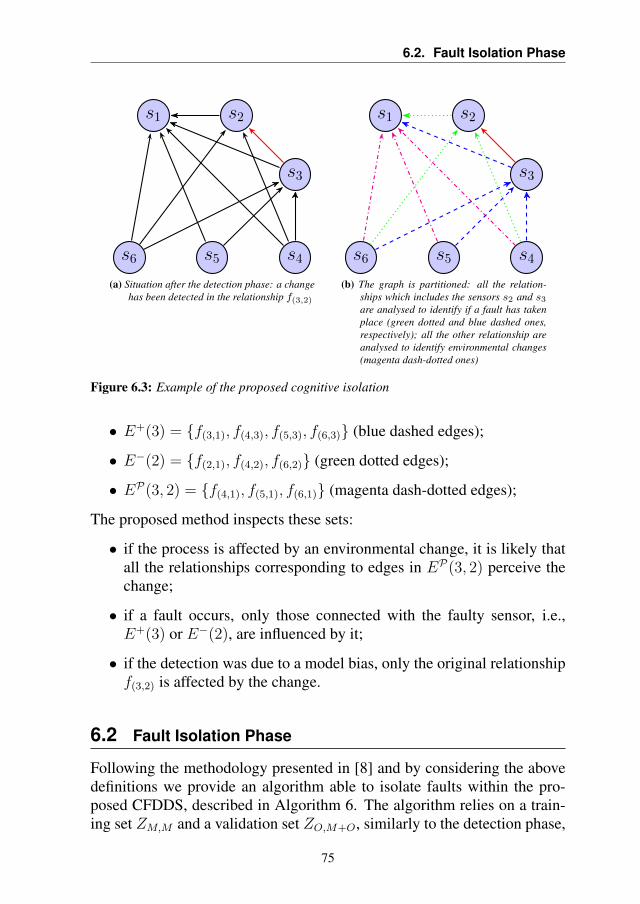
6.2. Fault Isolation Phase
s1 s2
s3
s4s5s6
(a) Situation after the detection phase: a changehas been detected in the relationship f(3,2)
s1 s2
s3
s4s5s6
(b) The graph is partitioned: all the relation-ships which includes the sensors s2 and s3are analysed to identify if a fault has takenplace (green dotted and blue dashed ones,respectively); all the other relationship areanalysed to identify environmental changes(magenta dash-dotted ones)
Figure 6.3: Example of the proposed cognitive isolation
• E+(3) = f(3,1), f(4,3), f(5,3), f(6,3) (blue dashed edges);
• E−(2) = f(2,1), f(4,2), f(6,2) (green dotted edges);
• EP(3, 2) = f(4,1), f(5,1), f(6,1) (magenta dash-dotted edges);
The proposed method inspects these sets:
• if the process is affected by an environmental change, it is likely thatall the relationships corresponding to edges in EP(3, 2) perceive thechange;
• if a fault occurs, only those connected with the faulty sensor, i.e.,E+(3) or E−(2), are influenced by it;
• if the detection was due to a model bias, only the original relationshipf(3,2) is affected by the change.
6.2 Fault Isolation Phase
Following the methodology presented in [8] and by considering the abovedefinitions we provide an algorithm able to isolate faults within the pro-posed CFDDS, described in Algorithm 6. The algorithm relies on a train-ing set ZM,M and a validation set ZO,M+O, similarly to the detection phase,
75
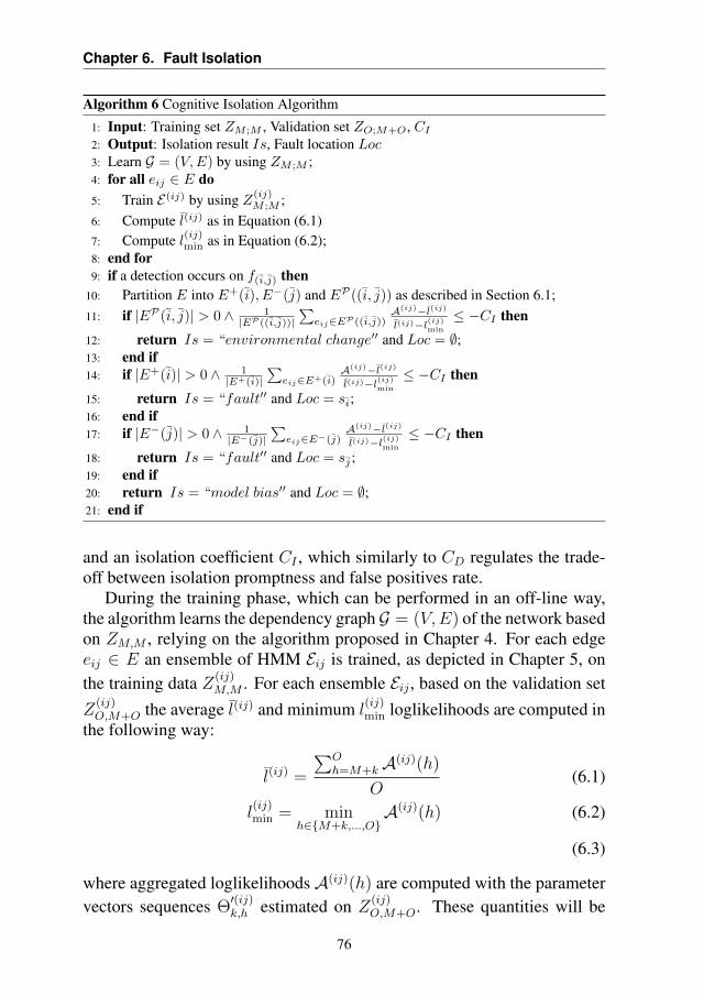
Chapter 6. Fault Isolation
Algorithm 6 Cognitive Isolation Algorithm
1: Input: Training set ZM ;M , Validation set ZO;M+O, CI2: Output: Isolation result Is, Fault location Loc3: Learn G = (V,E) by using ZM ;M ;4: for all eij ∈ E do5: Train E(ij) by using Z(ij)
M ;M ;6: Compute l(ij) as in Equation (6.1)7: Compute l(ij)min as in Equation (6.2);8: end for9: if a detection occurs on f(i,j) then
10: Partition E into E+(i), E−(j) and EP((i, j)) as described in Section 6.1;11: if |EP (i, j)| > 0 ∧ 1
|EP((i,j))|∑eij∈EP((i,j))
A(ij)−l(ij)
l(ij)−l(ij)min
≤ −CI then
12: return Is = “environmental change′′ and Loc = ∅;13: end if14: if |E+(i)| > 0 ∧ 1
|E+ (i)|∑eij∈E+ (i)
A(ij)−l(ij)
l(ij)−l(ij)min
≤ −CI then
15: return Is = “fault′′ and Loc = si;16: end if17: if |E−(j)| > 0 ∧ 1
|E−(j)|∑eij∈E−(j)
A(ij)−l(ij)
l(ij)−l(ij)min
≤ −CI then
18: return Is = “fault′′ and Loc = sj ;19: end if20: return Is = “model bias′′ and Loc = ∅;21: end if
and an isolation coefficient CI , which similarly to CD regulates the trade-off between isolation promptness and false positives rate.
During the training phase, which can be performed in an off-line way,the algorithm learns the dependency graph G = (V,E) of the network basedon ZM,M , relying on the algorithm proposed in Chapter 4. For each edgeeij ∈ E an ensemble of HMM Eij is trained, as depicted in Chapter 5, onthe training data Z(ij)
M,M . For each ensemble Eij , based on the validation setZ
(ij)O,M+O the average l(ij) and minimum l
(ij)min loglikelihoods are computed in
the following way:
l(ij) =
∑Oh=M+kA(ij)(h)
O(6.1)
l(ij)min = min
h∈M+k,...,OA(ij)(h) (6.2)
(6.3)
where aggregated loglikelihoodsA(ij)(h) are computed with the parametervectors sequences Θ
′(ij)k,h estimated on Z
(ij)O,M+O. These quantities will be
76
6.2. Fault Isolation Phase
used, as before, to evaluate the discrepancy of newly estimated parametervectors from the ensemble of HMM Eij characterizing the nominal state.
As soon as a detection occurs at time t on a specific functional relation-ship f(i,j), the algorithm partitions the dependency graph intoE+(i), E−(j)
and EP (i, j) and computes aggregated loglikelihoods A(ij)(t) for all eij ∈E. For each E ∈ E+(i), E−(j), EP (i, j), if it is not empty, we evaluatethe following expression:
1
|E|
∑eij∈E
A(ij) − l(ij)
l(ij) − l(ij)min
≤ −CI (6.4)
where | · | is the cardinality operator, CI < CD and CD is the coefficientfactor defined in Section 5.3.
At first, we apply the expression in Equation (6.4) to the partitionEP (i, j),to evaluate if a change in the environment has occurred. Otherwise, withthe similar procedure applied to E+(i) and E−(j), we try to isolate faultsin si and sj , respectively. If none of the above options are assessed, weconsider the detected change due to a model bias in the relationship f(i,j).
If an environmental change or a fault has been detected and isolated,the sensor network should be reconfigured, by training again the proposedCFDDS and by inspecting the damaged unit, respectively. Obviously, if theresult of the proposed isolation algorithm is Is = “modelbias′′, we need toestimate again the relationship which was affected by the change.
We would like to point out that the coefficient CI regulates how muchthe loglikelihood has to decrease before we consider it meaningful: an highvalue for CI will require a high loglikelihood drop to isolate a fault.
77

CHAPTER7Fault Identification
In this chapter we present the identification phase of the proposed CFDDS.On the basis of the techniques presented in the previous chapters, we sup-pose to have successfully detected a fault through the technique presentedin Chapter 5 and isolated it in a sensor si through the technique presentedin Chapter 6. After that, we would like to characterize the fault, for in-stance to understand if the fault already affected the system in the past or ifit presents new characteristics. The general scheme for the proposed iden-tification phase is presented in Figure 7.1. In this chapter, we consider afault-free dataset Z(ij)
M,M coming from a single data generating process Pand that faults affecting the system are of the abrupt type (see Section 2.2on fault modeling for details).
In Section 7.1 we propose the overall procedure adopted by the pro-posed CFDDS for fault identification, which is based on a newly developedevolving clustering technique. In Section 7.2 we detail the procedure forthe fault dictionary learning. Moreover, in Section 7.3 we discuss possibleextensions of the proposed framework to the case of incipient faults.
79
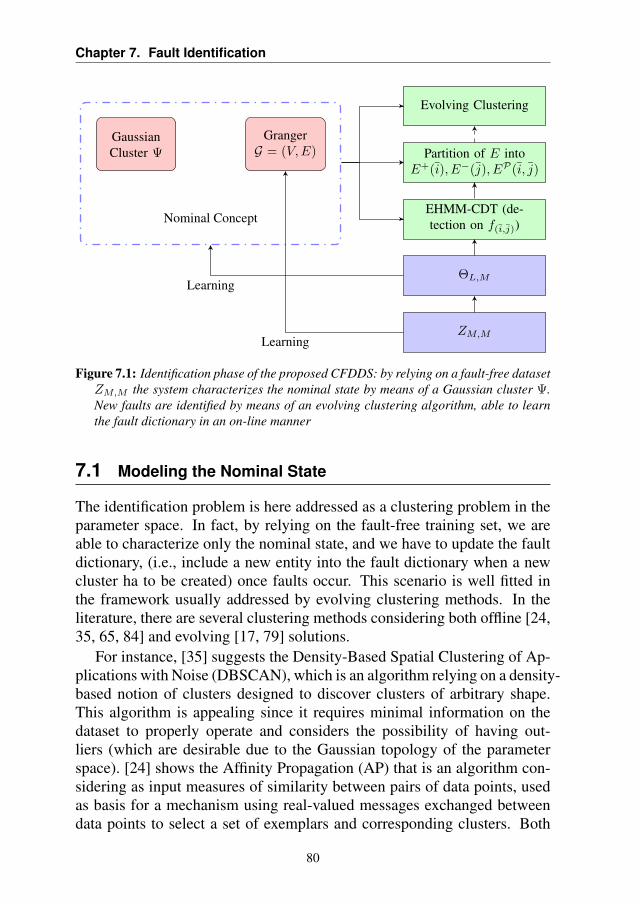
Chapter 7. Fault Identification
ZM,M
ΘL,M
EHMM-CDT (de-tection on f(i,j))
Partition of E intoE+(i), E−(j), EP (i, j)
Evolving Clustering
Nominal Concept
GrangerG = (V,E)
GaussianCluster Ψ
Learning
Learning
Figure 7.1: Identification phase of the proposed CFDDS: by relying on a fault-free datasetZM,M the system characterizes the nominal state by means of a Gaussian cluster Ψ.New faults are identified by means of an evolving clustering algorithm, able to learnthe fault dictionary in an on-line manner
7.1 Modeling the Nominal State
The identification problem is here addressed as a clustering problem in theparameter space. In fact, by relying on the fault-free training set, we areable to characterize only the nominal state, and we have to update the faultdictionary, (i.e., include a new entity into the fault dictionary when a newcluster ha to be created) once faults occur. This scenario is well fitted inthe framework usually addressed by evolving clustering methods. In theliterature, there are several clustering methods considering both offline [24,35, 65, 84] and evolving [17, 79] solutions.
For instance, [35] suggests the Density-Based Spatial Clustering of Ap-plications with Noise (DBSCAN), which is an algorithm relying on a density-based notion of clusters designed to discover clusters of arbitrary shape.This algorithm is appealing since it requires minimal information on thedataset to properly operate and considers the possibility of having out-liers (which are desirable due to the Gaussian topology of the parameterspace). [24] shows the Affinity Propagation (AP) that is an algorithm con-sidering as input measures of similarity between pairs of data points, usedas basis for a mechanism using real-valued messages exchanged betweendata points to select a set of exemplars and corresponding clusters. Both
80

7.1. Modeling the Nominal State
the algorithms presented above are not developed in an on-line framework.Their use in an on-line scenario would require a huge computational effort,since as soon as a new parameter vector is available they would requireto consider the whole dataset again. Differently, Evolving Cluster Method(ECM), described in [79], manages clusters with evolving strategies: it re-quires the setting of a parameterDthr, which is strictly related to the numberof clusters the algorithm will create during the operational life. None of theaforementioned methods is able to guarantee:
• a logic differentiation among clusters (i.e., those corresponding tonominal and fault states), inducing a different management on dif-ferent sets of cluster;
• the use of a Gaussian topology, required by the parameter space topol-ogy;
• an evolving mechanism able to manage newly estimated parametervectors.
Thus, we proposed a newly developed evolving clustering algorithm for theidentification phase, which takes advantage of temporal and spatial depen-dencies of the estimated parameters. For more details on alternative ap-proach to cognitive fault identification, other than clustering, the interestedreader can refer to Section 1.2.
For the identification phase, the proposed CFDDS relies on an initialtraining phase to characterize the nominal state Ψ by exploiting a fault-freetraining sequence Z(ij)
M,M . The dataset is windowed into non-overlappingbatches of length N , each of which is used to provide a parameter vectorestimate θ(ij)
t . The outcome is the sequence Θ(ij)L,M (L = M/N ).
The proposed algorithm is given in Algorithm 7. From results delineatedin Chapter 3 parameter vectors in Θ
(ij)L,M are distributed according to a Gaus-
sian distribution, provided that N is large enough, even though the systemis non-linear. Here we rely on a slightly different definition of cluster thandefinition 5.2.1. In this chapter we consider the following:
Definition 7.1.1. Given a parameter vectors sequence Θ(ij)L,M = θ(ij)
1 , . . . , θ(ij)L ,
where θ(ij)h is estimated on a dataset Z(i,j)
N,hN (non-overlapping batches),coming from a single process P , a Gaussian cluster Υ, induced by the
81

Chapter 7. Fault Identification
Algorithm 7 Evolving Clustering-Based Identification Algorithm
1: Data: Training set Z(ij)M,M ; αs, αm, ηt;
2: Results: Nominal cluster Ψ, Fault dictionary Φ;3: Compute mean θΨ and covariance matrix SΨ for the nominal state cluster4: Set nΨ = L and tΨ = L5: Set Φ = ∅ (φ = 0) and O = ∅6: while A new θ
(ij)t is available do
7: if Equation (7.6) holds Ψ then8: Associate θ(ij)
t to Ψ9: if |tΨ − t| ≤ ηt then
10: Update Ψ as in Equations (7.9) to (7.11)11: end if12: tΨ∗ ← t13: else14: if φ > 0 and Equation (7.6) holds for at least one Φr ∈ Φ then15: Select Φ∗ minimizing Equation (7.7)16: Associate θ(ij)
t to Φ∗
17: if |tΦ∗ − t| ≤ ηt then18: Update Φ∗ as in Equations (7.9) to (7.11)19: for θ
(ij)h ∈ O do
20: if Equation (7.6) holds for Φ∗ then21: Remove θ(ij)
h from outlier set O22: Associate θ(ij)
h to Φ∗
23: if |tΦ∗ − h| ≤ ηt then24: Update Φ∗ as in Equations (7.9) to (7.11)25: end if26: end if27: end for28: for Φr ∈ Φ,Φ 6= Φ∗ do29: if Equations (7.12) and (7.13) hold for Φ∗, Φr then30: Merge Φ∗, Φr as in Equations (7.14) to (7.17)31: end if32: end for33: end if34: tΦ∗ ← t35: else36: Insert θt in O37: Create O according to Algorithm 838: if O 6= ∅ then39: φ← φ+ 1
40: Create Φφ using θ(ij)k ∈ O
41: end if42: end if43: end if44: end while
82

7.1. Modeling the Nominal State
sequence Θ(ij)L,M , is a tuple (θΥ, SΥ, nΥ, tΥ), where:
θΥ =1
υ
∑θ∈Θ
(ij)L,M
θ, (7.1)
SΥ =1
υ − 1
∑θ∈Θ
(ij)L,M
(θ − θ)(θ − θ)T , (7.2)
nΥ = |Θ(ij)L,M | = υ, (7.3)
tΥ = L, (7.4)
and | · | is the cardinality operator.
Thanks to Equation (3.21) the nominal state Ψ can be described as aGaussian cluster composed by estimated parameter vectors, whose meanvector θΨ and covariance matrix SΨ can be estimated on Θ
(ij)L,M (Line 3).
For diagnosis purposes we assign to the nominal state the number nΨ ofparameter vectors used to estimate θΨ and SΨ and the last time instant tΨfor which a θ(ij)
t was associated to the nominal state Ψ. At the end of thetraining phase nΨ = L and tΨ = L (Line 4).
During the operational life, the proposed CFDDS estimates parametervectors from incoming non-overlapping N -sample data windows. The cor-responding estimated parameter vector θ(ij)
t is then either associated to thenominal state Ψ or to a generic r-th faulty one Φr present in the faultdictionary Φ = Φ1, . . . ,Φφ (φ represents the current number of faultyclasses in the fault dictionary). If the assignment cannot be granted accord-ing to a given confidence level, the estimated parameter vector θ(ij)
t is cur-rently considered an outlier and moved to an outlier set O. Similarly, other“housekeeping” operations are executed on the existing structures (outlierand faulty sets), e.g., leading to the merge of two faulty states, wheneverappropriate.
An example of the execution of the identification phase is provided inFigure 7.2. At the beginning, both the fault dictionary and the outlier setare empty (Figure 7.2a). They are populated during the operational lifeof the system, as data come in. The outlier set O is regularly inspectedto determine whether a new faulty state Φφ+1 needs to be generated byrelying on parameter vectors included in it (Figure 7.2b). If a parametervector cannot be associated to either the nominal state or one of the faultystates according to the given confidence level, it is considered an outlierand moved to the outlier set O (e.g., see the asterisks near the ellipse in theupper-right side of Figure 7.2d).
83

Chapter 7. Fault Identification
θ1
θ2
(a) The nominal state (crosses) is characterized dur-ing the training phase
θ1
θ2
(b) The number of outliers (asterisks) is increasingbut no faults are identified yet
θ1
θ2
(c) As soon as enough confidence is gathered for thepresence of a new faulty state, a new cluster iscreated (circles) and instances added to it
θ1
θ2
(d) When a different fault is identified (dots), it isadded to the fault dictionary.
Figure 7.2: Example of the identification phase in the proposed CFDDS
84

7.1. Modeling the Nominal State
Here, we assume that a fault affecting the optimal parameter θo (definedas in Section 3.3) abruptly moves the process from a stationary state to anew stationary one (abrupt fault). A faulty state Φr is hence characterizedby a mean vector θΦr and a covariance matrix SΦr , which can be estimatedfrom parameter vectors θ(ij)
h ∈ Φr. The proposed CFDDS stores the num-ber nΦr of vectors used to estimate θΦr and SΦr and the latest time instanttΦr where θ(ij)
h was associated to Φr.The distance between an estimated parameter vector θ(ij)
t and a clusterΥ can be computed by means of the Mahalanobis distance (as defined inSection 5.2):
m(θ(ij)t ,Υ) = (θΥ − θ(ij)
t )TS−1Υ (θΥ − θ(ij)
t ), (7.5)
where Υ ∈ Ψ,Φ1, . . . ,Φφ. Since Ψ and Φr ∈ Φ are Gaussian clusters,a neighbourhood centered in θΥ can be induced by containing those θ(ij)
t sbelonging to Υ with probability 1−αs [50], where αs is a given confidencelevel. More specifically, the spatial neighbourhood Rαs of a cluster Υ isdefines as:
Rαs =
θ | nΥ(nΥ − p)
p(n2Υ − 1)
m(θ,Υ) ≤ Fαs(p, nΥ − p)
(7.6)
holds, where Fαs(p, nΥ − p) is the quantile of order 1− αs of the Fisher’sdistribution with parameters p and nΥ − p. Similarly, a neighbourhoodis assigned to each cluster Υ ∈ Ψ,Φ1, . . . ,Φφ and constitutes the coreof the fault identification phase of the proposed CFDDS (Lines 7 and 14).The proposed CFDDS also contemplates the case of θ(ij)
t satisfying Equa-tion (7.6) for multiple clusters. In this case, θ(ij)
t is associated to the clusterΥ∗ (either nominal or faulty, Line 15):
Υ∗ = minΥ∈Ψ,Φ1,...,Φφ
nΥ(nΥ − p)p(n2
Υ − 1)m(θ
(ij)t ,Υ). (7.7)
In other words θ(ij)t is assigned to the nearest cluster, provided that con-
fidence 1 − αs is attained. Once Υ∗ has been determined, we set tΥ∗ = t(Lines 12 and 34). If θ(ij)
t cannot be associated either to Ψ, or to Φ1, . . . ,Φφ,it is considered to be an outlier and inserted in O (Line 36).
The algorithm, after taking into account the “spatial” locality betweenparameter vectors, analyses the “temporal” one, by evaluating to whichextent θ(ij)
t has been associated to Υ∗ (Lines 9 and 17), i.e.,
|tΥ∗ − t| ≤ ηt, (7.8)
85

Chapter 7. Fault Identification
where ηt ∈ N is a temporal threshold (when ηt = 1, the proposed CFDDSverifies if two consecutive time vectors θ(ij)
t and θ(ij)t−1 have been assigned to
the same cluster). This operation is important since we expect models builtover time to be temporally dependent.
If θ(ij)t satisfies both the spatial (Equation (7.6)) and the temporal (Equa-
tion (7.8)) membership conditions for a specific cluster Υ∗, it is inserted inthere and Υ∗ statistics are updated as follows (Lines 10 and 18):
θΥ∗ ←nΥ∗
nΥ∗ + 1θΥ∗ +
1
nΥ∗ + 1θ
(ij)t (7.9)
SΥ∗ ←nΥ∗ − 1
nΥ∗SΥ∗ +
nΥ∗ + 1
n2Υ∗
(θ(ij)t − θΥ∗)(θ
(ij)t − θΥ∗)
T (7.10)
nΥ∗ ← nΥ∗ + 1. (7.11)
The aforementioned procedure might update cluster Υr so that it partlyoverlaps with another one Υk. The proposed algorithm handles this sit-uation with a cluster merging procedure (Lines 28 to 30). The union ofclusters Υr and Υk is performed when the following two conditions arejointly satisfied,nΥr(nΥknΥr − nΥk − p+ 1)
(nΥk + 1)(nΥr − 1)pm(θΥr ,Υk) ≤ Fαm
2(p, nΥknΥr − nΥk − p+ 1)
(7.12)nΥk(nΥrnΥk − nΥr − p+ 1)
(nΥr + 1)(nΥk − 1)pm(θΥk ,Υr) ≤ Fαm
2(p, nΥrnΥk − nΥr − p+ 1),
(7.13)
i.e., if the cluster means θΥr and θΥk have probability greater than 1 − αmto belong to Υk and Υr, respectively. In Equations (7.12) and (7.13),Fαm
2(p, nΥknΥr − nΥk − p + 1) is the quantile of order 1 − αm/2 of the
Fisher’s distribution quantile with parameters p and nΥknΥr − nΥk − p +1. Approximated results for the confidence αm follow from the Bonfer-roni correction for multiple tests. If the above conditions are satisfied, theCFDDS merges the two clusters Υr and Υk to generate cluster Υ′ definedas:
θΥ′ ←nΥr
nΥr + nΥk
θΥr +nΥk
nΥr + nΥk
θΥk ; (7.14)
SΥ′ ← SΥr + SΥk +nΥrnΥk
nΥr + nΥk
(θΥr − θΥk)(θΥr − θΥk)T ; (7.15)
nΥ′ ← nΥr + nΥk ; (7.16)tΥ′ ← maxtΥr , tΥk. (7.17)
86

7.2. On-line Modeling the Fault Dictionary
The exact computation of the update for the covariance matrix is performedas in [66].
After a cluster update or the merge of two clusters, the proposed CFDDSchecks if parameter vectors in the outlier setO can now be associated eitherto the nominal state or to one of the faulty ones (Lines 19 to 24).
7.2 On-line Modeling the Fault Dictionary
We addressed so far the procedure allowing the insertion of the parametervectors into the nominal and faulty clusters and the merging of two faultyclusters. The remaining θ
(ij)t are collected into the outlier set O, where
further inspection is performed during the operational life of the system, toverify whether a new faulty state must be created or not.
With reference to Algorithm 8, a new cluster needs to be created depend-ing on the outcome of the KS test (Line 4). The test compares the empiricalCumulative Distribution Function (CDF) of all the θ(ij)
h s estimated by theproposed CFDDS during both the training and the operational phases andthe CDF induced by considering the estimated nominal state Ψ and faultystates Φ1, . . . ,Φφ. If the distribution of the θ(ij)
h s is no more coherentwith the current set of clusters, a new cluster must be created and a newfaulty class inserted in Φ. More in detail, the test is designed as:
H0 : F = FΓ vs. H1 : F 6= FΓ (7.18)
where F is the empirical CDF of all the θs and FΓ is the distribution inducedby Gaussian clusters Γ = Ψ,Φ1 . . .Φφ. The KS test statistics takes intoaccount the maximum distance between the two CDFs
Dp = max0≤α≤1
|F (Bα)− FΓ(Bα)|, (7.19)
where Bα is the region in the parameter space such that FΓ(Bα) = α(see [73] for further details). As stated in [73], Dp has the same distributionof the one-dimensional KS distribution, so, for the KS test, we can compareit with the asymptotic form of the KS distribution K [53, 78]. Given a con-fidence level αc, the critical region of the KS test (i.e., for rejecting the nullhypothesis H0) is composed by all Dp:
Dp > Kαc (7.20)
whereKαc is the quantile of order 1−αc of the one-dimensionalK distribu-tion. The proposed statistical test suffers from the curse of dimensionality,
87

Chapter 7. Fault Identification
i.e., it needs an exponentially increasing number of samples to be effec-tive as the parameter vectors dimension p increases. Therefore, if needed,we suggest to apply a dimensionality reduction method to the parametervectors θ(ij)
h ∈ O, e.g., based on PCA [50] or Random Projection (RP)method [23].
Once the KS test provides enough confidence to claim that a new clus-ter must be generated from the outlier set (i.e., hypothesis H0 is rejected),suitable instances are removed from O and the new cluster is created. Weassume the availability of a supervisor that is able to label new faulty clus-ters, e.g., by providing the type of encountered fault. This allows us forcreating online the fault dictionary. On the contrary, when the hypothesisH0 is not rejected, Algorithm 8 returns an empty set (Line 32).
It is worth noting that the Mahalanobis distance cannot be considered tomeasure the proximities between couples of parameter vectors in O, sincethe distribution of elements in the outlier set is unknown (i.e., we cannotassume that θ(ij)
h s ∈ O are Gaussian distributed as they are not). To addressthis issue we defined the spatial-temporal norm on θ(ij)
h , θ(ij)k ∈ O, inspired
by the metric suggested in [92]:
||θ(ij)h − θ(ij)
k ||2λ = λ
||θ(ij)h − θ(ij)
k ||2
2p+ (1− λ)
|h− k|t
(7.21)
where || · || is the euclidean norm, t is the last batch of data consideredand λ ∈ [0, 1] is a penalty factor balancing the spatial locality and thetemporal one. A normalization procedure is required so that both the spatialand temporal components of the norm are constrained to the [0, 1] interval.The proposed CFDDS adopts the online normalization procedure describedin [48].
To select parameter vectors for the new cluster, we apply to the outlierset O the Mountain Method (MM) [83, 85, 87], which identifies the densitycenter for the θ(ij)
h s, θ(ij)h ∈ O (Lines 7 to 12). Finally, this algorithm
estimates the density as:
ΩRMM(ck, θ(ij)h ; r) = exp
(−||θ
(ij)h − ck||2λ
2r2
)(7.22)
where ck ∈ Rp is a center and r is an influence radius parameter. Thealgorithm iteratively approximates:
c∗ = maxc
∑θ(ij)h ∈O
ΩRMM(c, θ(ij)h , r). (7.23)
88

7.2. On-line Modeling the Fault Dictionary
The potential function ΩRMM is robust to outliers (see [87] for a formalproof) and, since it decreases slowly when ||θ(ij)
h − ck||λ < r and fast if||θ(ij)
h − ck||λ > r, it defines a neighbourhood around each class centerck. For the purpose of the cluster creation a center will be initialized foreach parameter vector θ(ij)
h ∈ O. As described in [85], ηi of Algorithm 8represents both a tolerance threshold for the convergence of the iterativeprocedure to identify the cluster center and the maximum error of the opti-mization procedure. As one might imagine the method is rather sensitive tor, which highly influences the clustering results. Here, we suggested threedifferent heuristics to identify a suitable value for the radius r:
• power estimate using correlation [87];
• median distance criterion [83];
• maximum edge length of minimum spanning tree under the normaldistribution hypothesis [67].
At the end of the mountain method each parameter vector is associatedwith a set Os (Lines 14 to 15) and O, the set characterized by the largestcardinality, is selected as a new candidate cluster.
To identify the cluster shape of O (we do not have a priori informationabout the covariance matrix of the novel cluster), a Minimum CovarianceDeterminant search method [40] is executed (Lines 16 to 29), i.e., a sub-set of elements O ⊆ O is selected s.t. the determinant of the parametercovariance is minimal. This method can be applied when the number ofsamples in O ≥ p. When this condition is satisfied (Line 16), a new clusteris created: the mean and the covariance of the parameter vectors in O arecomputed, nΦφ+1
= |O|, tΦφ+1= maxθh∈O h and the algorithm returns O
(Line 27). Otherwise, when O < p, the algorithm returns the empty set ∅(Line 29).
Note that the algorithm requires at least nΥ = p + 1 parameter vectorsto create a cluster. More parameter vectors would allow a better character-ization of the cluster itself since the variance of the estimation of the meanand the covariance matrix scales asymptotically as 1
nΥ. Moreover, as time
passes, more and more parameter vectors are inserted into the outlier set.To reduce as much as possible the creation of false faulty classes we shouldconsider an oblivion coefficient on the parameter vectors in the outlier set ormechanisms to discard the oldest ones (e.g., by setting a maximum value onthe cardinality of the outlier set and keeping the new ones). The algorithmcan be easily modified to take into account this case.
89

Chapter 7. Fault Identification
Algorithm 8 Faulty Cluster Creation Algorithm
Data: Outlier set O; Clustering Γ; αc, ηi;Results: Faulty cluster O;Compute Dp according to Equation (7.20)if Dp > Kαc then
Set ch = θ(ij)h , ∀θ(ij)
h ∈ O and err ≥ ηiCompute rwhile err ≥ ηi do
for k s.t, θ(ij)k ∈ O do
ck ← ck
ck ←
∑θ(ij)h ∈O ΩRMM (ck, θ
(ij)h ; r)θ
(ij)h∑
θ(ij)h ∈O ΩRMM (ck, θ
(ij)h ; r)
end forerr = max
k||ck − ck||λ
end whileAssociate all centers ck, ch s.t. ||ck − ch||λ ≤ 2ηi to a set, creating the setsO1, . . . , OSLet O = arg maxs∈1,...,S |Os|, i.e., the set with the largest cardinalityif |O| ≥ p then
Choose randomly h = |O|+p+12 elements in O to define O
Set S∗ =∑θ(ij)h ∈O
(θ(ij)h −c∗)(θ(ij)h −c∗)T
h−1
while O 6= O′ doO′ ← Ofor θ(ij)
h ∈ O dod(θ
(ij)h ) = (θ
(ij)h − c∗)(S∗)−1(θ
(ij)h − c∗)T
end forO ← arg minO′⊆O,|O′|=h
∑θ(ij)h ∈O′ d(θ
(ij)h )
S∗ ←∑θ(ij)h ∈O
(θ(ij)h −c∗)(θ(ij)h −c∗)T
h−1
end whilereturn O
elsereturn O = ∅
end ifelse
return O = ∅end if
90

7.3. Dealing with Incipient Faults
7.3 Dealing with Incipient Faults
One of the main assumption of the proposed identification phase is thatfaults abruptly moves the process from a stationary state to a new stationaryone (abrupt faults). This is due to the fact that only stationary states induce aGaussian topology in the parameter space (see Section 3.3 for more details),while there are no theoretical results for different kind of faults. Thus, if theassumption that only abrupt faults occur does not hold, situation differentfrom those previously described may appear in the parameter space, whereparameter vectors are not identically distributed anymore. Some examples,where the faults have incipient development are presented in Figure 7.3.
In particular, Figure 7.3a presents the situation where the fault has anincipient development and, after that, it stabilizes into a stationary state(incipient permanent fault). In this case, the identification phase of theproposed CFDDS is still able to deal with this situation, provided that astrong evidence for the creation of the cluster is provided. For instance, wecould impose a stronger condition for the cluster creation procedure, likerequiring to have at least p >> p+1 to allow the formation of a new cluster.
When the fault induces a set of continuously drifting parameter vectors,as in Figure 7.3b, the ability to characterize a fault in the parameter spaceseem to be not viable anymore. Moreover, in this case the analysis shouldbe carried on the trajectory the parameter vectors are following, for instanceby relying on joint information on its temporal and spatial evolution (speedand acceleration in the parameter space).
When the process slowly drifts in the parameter space from a station-ary state to another, as in Figure 7.3c, it may happen that the nominal andthe faulty clusters significantly overlap. If we are expecting such a phe-nomenon, a conservative solution is to fix the nominal state at the end ofthe training phase (i.e., we do not update its estimated mean θΨ and covari-ance matrix SΨ if a new parameter vector belonging to the nominal state isspotted). With this approach we avoid to include parameter vectors belong-ing to a fault into the nominal cluster.
91

Chapter 7. Fault Identification
θ1
θ2
(a) The transition phase (for instance,given by an incipient fault) is fastand the fault stabilizes in a station-ary state
θ1
θ2
(b) The fault is rapidly changing (for in-stance, a continuous drift) and theevolving algorithm is not able tocharacterize it. Its parameter vec-tors form a trajectory in the param-eter space)
θ1
θ2
(c) Slowly drifting fault, which overlapswith the nominal state
Figure 7.3: Example of different incipient faults in the parameter vectors space
92

CHAPTER8CFDDS Implementation
In this chapter, we report a brief overview of the main functions imple-menting the previously described phases of the proposed CFDDS, whichare considered in Chapter 9 to validate the proposed framework. The codedeveloped within this dissertation is available at [2].
Two external toolboxes were considered within the libraries developed:one for the estimation of the HMM and one for the multivariate grangercausality toolbox [18]. The library implementing the proposed CFDDS isstructured as follows:
• data generation procedures (data_gen directory)
• parameter vectors estimation (model_estimation directory)
• graph learning phase(cogn_net directory)
• detection and isolation phases (cogn_hmm directory)
• identification phase (cogn_fds directory)
93

Chapter 8. CFDDS Implementation
Data Generation
opts_generation: generates the options for the input, output andfault generation procedures. It needs as input two structures describing thestructure of the signal to be simulated and the fault signature.
input_generation: generates an input for a discrete time dynamicprocess. The function allows to generate data from a cosinusoidal func-tion with additive noise, from a Gaussian random walk process or from auniform distribution over [−1, 1].
signal_generation: generates the output of a discrete time dy-namic process, given the exogenous input and specifics about the dynamicmodel to take into account. It is possible to choose among a linear ARXmodel, a pendulum and a Van der Pol oscillator [51].
fault_generation: injects faults in a given signal. It allows toinsert structured (with dynamic φ(t) = f(x, y)) faults, as well as non struc-tured ones (φ(t) = φ, φ ∈ R).
Parameter Estimation
idarmax: estimates the orders of a given model family (e.g., ARX),based on a given dataset. It allows to consider a specific range of ordersand to choose the criterion used for the selection (e.g., Akaike InformationCriterion (AIC), Mean Square Error (MSE) on a validation set).
model_creation: estimates model parameter vectors from an input-output dataset (x(t), y(t))Nt=1 given the orders of the linear dynamic sys-tem to consider.
Graph Learning
sel_rel: learns the dependency graph from a fault-free dataset, bychoosing among different methods (e,g,. correlation analysis and Granger-based statistical test).
granger: implements the Granger-based test for assessing the multi-variate Granger causality in a multivariate dataset.
Detection Phase
train_hmm_fds: estimate the parameters of a HMM or an ensembleof HMMs relying on a given training dataset. It requires also to specify thebinary relationships which should be considered, i.e., it requires to have a
94

dependency graph in order to decide which set of relationships to take intoaccount.
test_hmm_fds: given a model trained with train_hmm_fds anda stream of data, it computes the loglikelihood for each trained HMM andfor each relationship considered during training.
plot_lls: given a model tested with test_hmm_fds it is able toplot the computed loglikelihood for the data provided during the testingphase.
hmm_fds_detection: given a HMM model and an aggregation method,it is able to compute the detection result for a single functional relationship.
detection_net: aggregates the results provided by hmm_fds_detectionand checks the consistency of the previously provided results.
Isolation Phase
fds_isolation: is able to perform the isolation phase of the pro-posed CFDDS, given the loglikelihoods provided by HMMs on differentfunctional relationships.
Identification Phase init_clu: initializes an empty clustering structure,able to store both the cluster representing the nominal state of the systemand the ones representing the faulty states.
clust_train: populates the nominal cluster and updates its statis-tics.
clust_evol: core of the evolving algorithm described in Algorithm 7.Given an estimated parameter vector, it is able to automatically decide toassign it to the nominal state, to a faulty one or to the outlier set, as wellas to create new cluster, merge the old ones if necessary and update theirstatistics.
95

CHAPTER9Experimental Results
In this chapter, we analyse the performance of the proposed CFDDS ona synthetically generated dataset, a real benchmark coming from sensornetworks designed to perform an environmental monitoring task and a sim-ulated one based on data coming from a sensor network inspecting a wa-ter distribution system. We here considered each phase of the proposedCFDDS one at a time, to evaluate separately the advantages each phase isproviding to the overall framework. The chapter is structured as follows: atfirst an overview of the considered datasets is presented in Section 9.1. Af-ter that the phases of the proposed CFDDS are tested on the aforementioneddatasets in Sections 9.2 to 9.5. Finally, general remarks on the describedexperimental campaign are provided in Section 9.6.
9.1 The Considered Datasets
9.1.1 Application D1: Synthetic Datasets
Here, we consider datastreams coming from a synthetically generated sen-sor network with randomly generated relationships among datastreams. Togenerate these data, a directed acyclic graph, representing the dependency
97

Chapter 9. Experimental Results
graph of the existing functional relationships (with a fixed amount of nodesand a fixed number of edges) is generated. After that, for all those sen-sors without any incoming edge, we generate samples by relying on thefollowing autoregressive process:
xi(t) = φxi(t− 1) + ψ(t) (9.1)
where φ = 0.4, ψ(t) ∼ N (0, 0.1), η(t) is an uncorrelated white noises.t. η(t) ∼ N (0, σ2) and σ is the standard deviation of the noise. Then,by considering a topological order of the graph1, datastreams are generatedeither through linear L or sinusoidal S models as:
L : xj(t) = θTj z + η(t); (9.2)
S : xj(t) = sin(θTj z
)+ η(t), (9.3)
where:
z =[xj(t− 1), xj(t− 2), xi1j(t− 1), xi1j(t− 2),
. . . , xinj(t− 1), xinj(t− 2)]
(9.4)
z ∈ R2(1+nj) is the vector of the autoregressive (xj(t − 1), xj(t − 2)) andexogenous (xi1j(t − 1), . . . , xinj(t − 2)), i1j, . . . inj components, is theset of the indexes of those sensors s∗ s.t. exists an edge (s∗, sj) in thegraph, i.e., the indexes of the sensors s∗ with an edge from s∗ to sj , andθj ∈ R2(1+nj) is a randomly generated vector.
s1 s2
s3
s4s5s6
Figure 9.1: Example of generation of the dependency graph for a network with n = 6sensors.
1Any of the possible topological orders provides the same results for what it concerns the generation of thedatastreams.
98

9.1. The Considered Datasets
For instance in the graph of Figure 9.1, we generate at first the datas-treams x6, x5 or x4 from Equation (9.1) (in any order). After that, by fol-lowing the topologic order of the graph, we generate x3 from either Equa-tion (9.2) or Equation (9.3) by considering as input streams x6, x5 and x4.By using the same model chosen to generate x3, we generate x2 (using asinput x6, x4 and x3) and x1 (using as input all the other streams).
9.1.2 Application D2: Rialba Dataset
In this application data are gathered from a rock collapse and landslideforecasting system, [5, 6] deployed at the Towers of Rialba site, in North-ern Italy. The sensor network deployment area is inspecting a limestone-conglomerate rock divided by a system of fractures. The towers are closeto the main civil infrastructures connecting Lecco and Sondrio provinces(speedway, railway, gas, and electric distribution networks). The monitor-ing system consists of three sensing and processing units and a base sta-tion and has been active since July 7th, 2010. The base station relies on aUniversal Mobile Telecommunications System (UMTS) modem for remotedata and commands communication with the Intelligent Embedded Systemlab.
This dataset is available at [1]. The sampling period of the provideddata is 5 minutes. We would like to point out that this scenario representsa particularly challenging application of the techniques developed withinthis dissertation, since it is hard to infer a precise analytical model of theobserved phenomenon.
0.5 1 1.5 2 2.5 3 3.5
x 104
0.21
0.215
0.22
0.225
0.23
0.235
0.24
0.245
Clinometer 2
Clinometer 1
Sample
Figure 9.2: The measurements acquired from two clinometers of the monitoring systemdeployed at the Towers of Rialba.
An example of the data coming from this application are presented in
99

Chapter 9. Experimental Results
Figure 9.2, in particular here we show the measurements coming from twoclinometers deployed in two different units of the sensor network.
9.1.3 Application D3: Barcelona Water Distribution Network SystemDataset
Figure 9.3: Scheme for the BWNDS
The second testbed refers to data generated from the BWNDS simulator[25], whose scheme is provided in Figure 9.3. By relying on a networkof 17 tanks, 26 pumps, 35 valves, 9 external sources of the BWNDS, thissimulator allows to artificially inject faults in a specific flow sensor of thenetwork, by specifying the fault signature, the fault magnitude and the faulttime-horizon. This simulator has been developed in MATLAB/SIMULINKenvironment, using a model calibrated and validated with real data provid-ing a good degree of representativeness of the actual network behaviour.
9.2 Dependency Graph Learning
The aim of this section is to evaluate the performance of the proposeddependency graph learning phase using both data synthetically generated(Application D1) and coming from a real-world sensor network for rockcollapse and landslide forecasting (Application D2). In particular, two dif-ferent objectives have been considered and evaluated:
• the ability to correctly identify the meaningful relationships existingamong the acquired datastreams;
• the fault detection performance of the HMM-CDT relying on the learnedGranger-based dependency graph.
100

9.2. Dependency Graph Learning
Figures of Merit With respect to the ability to identify the correct relation-ships in acquired datastreams, we consider the following figures of merit:
• Recall R = |Er∩E||Er| : fraction of correctly selected functional relation-
ships that are present in the learned dependency graph;
• Precision P = |Er∩E||E| : fraction of functional relationships in the learned
dependency graphed that are correctly selected,
where Er is the set of truly existing relationships among acquired data and| · | is the cardinality operator.
Differently, for the evaluation of the fault detection performance, weconsider the following figures of merit:
• False Positive rate (FP ): fraction of experiments in which the detec-tion of the change happened before the change occurred;
• False Negative rate (FN ): fraction of experiments where no changewas detected in the relationship affected by the fault (or environmentalchange);
• Detection Delay (DD): number of samples necessary to detect a change,if no false positive detection occurred.
Comparison To compare the performance of the proposed dependency graphlearning phase, we considered the correlation analysis adopted in [8]. Morespecifically we considered the maximum (w.r.t. different time lags) of thecrosscorrelation between couples of datastream and we consider the rela-tionship only if its value was higher than the chosen threshold ρ, 0 < ρ < 1.In particular, we considered three different values of the crosscorrelationthreshold: high crosscorrelation (i.e., ρhigh = 0.9), low crosscorrelation(ρlow = 0.02) and best crosscorrelation (ρbest defined as the highest value ofcrosscorrelation that allows to consider all the truly existing relationshipsin the dependency graph). Obviously, the best crosscorrelation thresholdcannot be a priori set (since it requires the knowledge of the true relation-ships present within the network) and, hence, it represents the correct valuefor the threshold. We verified a posteriori that the high and low values ofthe threshold have been properly set, since they actually were higher andlower than the value considered for the best one ρbest, respectively.
Parameters Configuration The confidence on the Granger-based test is set toαg = 0.05. The parameters of the HMM-CDT have been assigned as fol-lows: N = 100, k = 10, the best configuration for the HMMs was selected
101

Chapter 9. Experimental Results
by considering s ∈ 3, . . . , 6 hidden states and the number of GMMs isin 1, 2, 4, 8, 16, 32. The orders of the Single Input Single Output (SISO)ARX models are chosen through a model selection procedure based on themean square error on a validation set.
9.2.1 Application D1: Synthetic Dataset
Experimental Setting Here, we consider a sequence of 7145 samples gener-ated from S or L with n = 6, |E| = 6 and the first M = 4085 used forthe training and validation phase, while the remaining ones constitute thetest set for the detection phase. In the experiments regarding the ability tocorrectly identify the meaningful relationships existing in acquired datas-treams, we considered 20 equally spaced noise levels σ ∈ [0.05∆i, . . . ,∆i],where ∆i = maxt xi(t)−mint xi(t). Differently, in the experiments on thefault detection performance, an additive constant abrupt fault:
A(2) φi(t) =
0.2∆i t > t
0 otherwise
has been injected at time instant t = 5309 on each sensor one at a time (tomodel a sensor fault) and on all the sensors at the same time (to model achange in the environment2). Results are averaged over the different faultsand repeated over 100 runs.
Results The experimental results on the ability to correctly identify themeaningful relationships are presented in Figures 9.4 to 9.7. As expected,the choice of the threshold value for the crosscorrelation analysis is critical.In fact, it is possible to see that the choice of a low correlation threshold ρlowimplies the selection of |E| ≈ 30 relationships, leading to a recall R ≈ 1.As expected, the drawback of this solution is the fact that the precisionP ≈ 0.4, thus the method is considering several non-relevant relationships.Conversely, the main drawback of the high correlation threshold ρhigh is thefact that relevant relationships might not be included into the dependencygraph. More specifically, when σ > 0.1, the correlation analysis methoddoes not select any relationship. As expected, by analysing Figure 9.8, wecan see that the best correlation value ρbest decreases as noise increases.Thus, one should rely on a priori information about the noise level to beable to set the proper threshold for the correlation analysis. Conversely, the
2Here, we consider the simplifying assumption that the injected change propagates instantly though the sensornetwork.
102
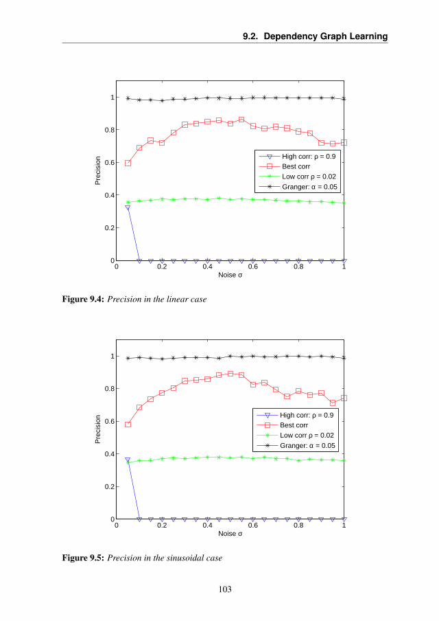
9.2. Dependency Graph Learning
0 0.2 0.4 0.6 0.8 10
0.2
0.4
0.6
0.8
1P
reci
sion
Noise σ
High corr: ρ = 0.9Best corr
Low corr ρ = 0.02
Granger: α = 0.05
Figure 9.4: Precision in the linear case
0 0.2 0.4 0.6 0.8 10
0.2
0.4
0.6
0.8
1
Pre
cisi
on
Noise σ
High corr: ρ = 0.9Best corr
Low corr ρ = 0.02
Granger: α = 0.05
Figure 9.5: Precision in the sinusoidal case
103

Chapter 9. Experimental Results
0 0.2 0.4 0.6 0.8 10
0.2
0.4
0.6
0.8
1
Rec
all
Noise σ
High corr: ρ = 0.9Best corr
Low corr ρ = 0.02
Granger: α = 0.05
Figure 9.6: Recall in the linear case
0 0.2 0.4 0.6 0.8 10
0.2
0.4
0.6
0.8
1
Rec
all
Noise σ
High corr: ρ = 0.9Best corr
Low corr ρ = 0.02
Granger: α = 0.05
Figure 9.7: Recall in the sinusoidal case
104

9.2. Dependency Graph Learning
0.1 0.2 0.3 0.4 0.5 0.6 0.7 0.8 0.9 10
0.2
0.4
0.6
0.8
Noise σ
Bes
t cor
rela
tion
0.1 0.2 0.3 0.4 0.5 0.6 0.7 0.8 0.9 10
0.2
0.4
0.6
0.8
Noise σ
Bes
t cor
rela
tion
Figure 9.8: Box-plot for the best correlation: the linear L (top) and sinusoidal S (bottom)cases
proposed dependency graph learning phase based on Granger causality isable to maintain acceptable values for both precision and recall (P ≈ 1,equal to the one obtained by choosing ρlow, and R > 0.7) without any apriori information about the noise level.
Results about fault detection are shown in Table 9.1. We consideredthree different noise levels σ ∈ 0.05, 0.1, 0.3 and three different valuesof the parameter C for the HMM-CDT, to allow a fair comparison amongthe proposed Granger-based framework (identified from now on with G),the crosscorrelation algorithm with ρlow and the crosscorrelation algorithmwith ρbest (the one with ρhigh is not considered here). More specifically,Cgran is the smallest parameter that allows to have FP = 0 for the HMM-CDT based on the Granger-based dependency graph. Similarly Cbest andClow are the ones allowing to have FP = 0 for the HMM-CDT based oncorrelation analysis graph, by using ρbest and ρlow, respectively, as thresh-olds for the crosscorrelation. By looking at the experiments on the lin-ear function L with σ = 0.05, we can see that, with Cgran, the Granger-based solution provides DD and FN similar to the ones obtained withρbest (DD = 49.7 and FN = 0.113 for G, DD = 49.2 and FN = 0.079for ρbest), and G provides a lower FP (FP = 0 for G and FP = 0.41 forρbest) without requiring any a priori information about the network or thenoise level.
By comparing the proposed Granger-based framework with correlation
105

Chapter 9. Experimental Results
Table 9.1: Detection results for Application D1
Lin
earf
unct
ionL
σ = 0.05 σ = 0.1 σ = 0.3Cgran = 4.5 Cgran = 4.9 Cgran = 4.8
ρbest ρlow G ρbest ρlow G ρbest ρlow G|E| 10.1 16.3 6.0 8.3 16.0 6.1 7.3 15.9 6.0DD 49.2 65.0 49.7 87.4 93.6 85.7 130.3 131.9 132.1FN 0.079 0.044 0.113 0.126 0.064 0.181 0.307 0.104 0.354FP 0.410 0.650 0.000 0.280 0.610 0.000 0.120 0.620 0.000
Cbest = 5.2 Cbest = 5.2 Cbest = 5.0|E| 10.1 16.3 6.0 8.3 16.0 6.1 7.3 15.9 6.0DD 56.7 62.0 56.9 88.5 103.2 92.1 124.8 127.6 133.0FN 0.117 0.061 0.129 0.180 0.080 0.206 0.351 0.129 0.359FP 0.000 0.390 0.030 0.000 0.460 0.020 0.000 0.530 0.020
Clow = 6.0 Clow = 6.3 Clow = 6.2|E| 10.1 16.3 6.0 8.3 16.0 6.1 7.3 15.9 6.0DD 63.1 63.4 62.3 109.6 110.7 112.3 149.0 134.8 156.1FN 0.139 0.093 0.154 0.217 0.140 0.247 0.434 0.259 0.450FP 0.000 0.000 0.020 0.000 0.000 0.000 0.000 0.000 0.000
Sinu
soid
alfu
nctio
nS
σ = 0.05 σ = 0.1 σ = 0.3Cgran = 5.1 Cgran = 5.1 Cgran = 4.6
ρbest ρlow G ρbest ρlow G ρbest ρlow G|E| 10.0 16.1 6.0 9.0 16.0 6.0 7.4 15.8 5.9DD 47.5 51.5 49.0 84.3 84.5 82.2 112.0 127.0 14.9FN 0.081 0.043 0.121 0.111 0.047 0.177 0.256 0.076 0.317FP 0.350 0.610 0.000 0.360 0.660 0.000 0.200 0.670 0.000
Cbest = 5.7 Cbest = 5.7 Cbest = 5.0|E| 10.0 16.1 6.0 9.0 16.0 6.0 7.4 15.8 5.9DD 53.8 60.2 55.2 83.7 86.5 90.1 115.0 127.8 123.3FN 0.110 0.057 0.136 0.179 0.076 0.200 0.311 0.114 0.346FP 0.000 0.360 0.030 0.000 0.410 0.030 0.000 0.500 0.000
Clow = 6.7(2.3) Clow = 6.5(4.0) Clow = 6.4(2.2)|E| 10.0 16.1 6.0 9.0 16.0 6.0 7.4 15.8 5.9DD 61.5 61.3 63.5 89.9 91.7 95.0 143.9 129.5 152.2FN 0.127 0.103 0.156 0.203 0.131 0.236 0.383 0.239 0.421FP 0.000 0.000 0.000 0.000 0.000 0.020 0.000 0.000 0.000
106
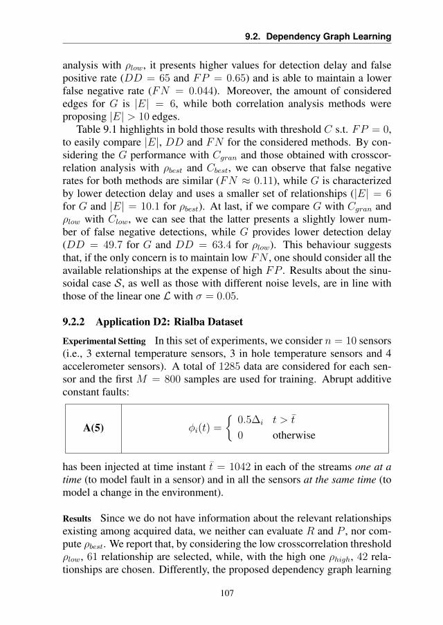
9.2. Dependency Graph Learning
analysis with ρlow, it presents higher values for detection delay and falsepositive rate (DD = 65 and FP = 0.65) and is able to maintain a lowerfalse negative rate (FN = 0.044). Moreover, the amount of considerededges for G is |E| = 6, while both correlation analysis methods wereproposing |E| > 10 edges.
Table 9.1 highlights in bold those results with threshold C s.t. FP = 0,to easily compare |E|, DD and FN for the considered methods. By con-sidering the G performance with Cgran and those obtained with crosscor-relation analysis with ρbest and Cbest, we can observe that false negativerates for both methods are similar (FN ≈ 0.11), while G is characterizedby lower detection delay and uses a smaller set of relationships (|E| = 6for G and |E| = 10.1 for ρbest). At last, if we compare G with Cgran andρlow with Clow, we can see that the latter presents a slightly lower num-ber of false negative detections, while G provides lower detection delay(DD = 49.7 for G and DD = 63.4 for ρlow). This behaviour suggeststhat, if the only concern is to maintain low FN , one should consider all theavailable relationships at the expense of high FP . Results about the sinu-soidal case S, as well as those with different noise levels, are in line withthose of the linear one L with σ = 0.05.
9.2.2 Application D2: Rialba Dataset
Experimental Setting In this set of experiments, we consider n = 10 sensors(i.e., 3 external temperature sensors, 3 in hole temperature sensors and 4accelerometer sensors). A total of 1285 data are considered for each sen-sor and the first M = 800 samples are used for training. Abrupt additiveconstant faults:
A(5) φi(t) =
0.5∆i t > t
0 otherwise
has been injected at time instant t = 1042 in each of the streams one at atime (to model fault in a sensor) and in all the sensors at the same time (tomodel a change in the environment).
Results Since we do not have information about the relevant relationshipsexisting among acquired data, we neither can evaluate R and P , nor com-pute ρbest. We report that, by considering the low crosscorrelation thresholdρlow, 61 relationship are selected, while, with the high one ρhigh, 42 rela-tionships are chosen. Differently, the proposed dependency graph learning
107

Chapter 9. Experimental Results
phase selects 19 relationships. Interestingly, 12 over 19 of those relation-ships are in common with the high crosscorrelation selection and 15 are incommon with the low crosscorrelation one.
Table 9.2: Detection results for Application D2: the numeric values are detection delaysDD for different dependency graph learning algorithms, while FP and FN standsfor false positive and false negative detections, respectively.
Cgran = 1.271 Chigh = Clow = 3.141DD DD
Faulty sensor G ρhigh ρlow G ρhigh ρlows1 1 FP FP 2 2 2s2 1 FP FP 7 7 3s3 1 FP FP 7 1 1s4 1 FP FP 2 2 1s5 2 FP FP FN 8 8s6 2 FP FP 6 3 3s7 1 FP FP 2 2 1s8 2 FP FP 55 55 9s9 2 FP FP 5 5 5s10 1 FP FP 3 1 1All 1 FP FP 1 1 1
Results for the detection phase are provided in Table 9.2. The HMM-CDT parameter C is here set to Cgran = 1.271 and Chigh = Clow = 3.141,which are the smallest values s.t. FP = 0 by considering the Granger andcorrelation analysis approaches, respectively. The Granger-based methodis able to maintain a DD generally better than the one provided by the cor-relation analysis. Is it also possible to see that in the case of fault located insensor s5 the Granger-based framework does not provide a detection (FN ),supporting the idea that one should select a high number of relationships tomaintain a low FN , at the expense of an increase in the FP .
9.3 Detection Phase
To evaluate the detection performance of the proposed proposed CFDDSbased on the EHMM-CDT algorithm we considered the synthetic (Appli-cation D1) and a real data scenario (Application D2). Here the specificaim is the to test the proposed CFDDS to assess its detection promptnessand accuracy, in terms of false positive, false negative rates and detectiondelays.
108
9.3. Detection Phase
Figures of Merit To evaluate the detection ability of what proposed, the fol-lowing figures of merit have been considered:
• False Positive rate (FP ): fraction of the experiments where the methoddetected a change before it actually appears;
• False Negative rate (FN ): fraction of the experiments where the methoddid not detected a change;
• Detection Delay (DD): the number of samples necessary to detect achange.
Comparison The detection phase of the proposed CFDDS is compared withthe HMM-CDT, where a single HMM was considered (the one with largestloglikelihood on a validation set among those considered for the ensemble).
Parameters Configuration As regards the model family M, we consideredSISO LTI ARX models, whose orders are chosen through a model selec-tion procedure, i.e., minimizing the mean square one-step-ahead predictionerror on a validation set. The HMMs are configured by considering batchesof N = 100 samples, parameter vector sequences of length k = 10 andexploring the space of HMMs with s ∈ 3, . . . , 6 hidden states and with1, 2, 4, 8, 16, 32 Gaussian distributions in each GMM. The cardinality ofthe ensemble was set to Q = 30. Finally, the parameter vectors estimationis performed with the LS method.
9.3.1 Application D1: Synthetic Dataset
Experimental Setting The data for the synthetic application have been gener-ated from S with n = 2 sensors, where θ2 ∈ [0, 1]33, σ ∈ 0.01∆2, 0.05∆2,where ∆2 = maxt x2(t)−mint x2(t). Each experiment lasts 6125 samples,where M = 3268 are used for training, O = 817 for validation and 2040for testing. Results are averaged over 1000 independent runs.
To assess the detection abilities of the detection phase for the proposeCFDDS, we injected five different kinds of abrupt permanent faults startingat time instant t = 5105:
3In this set of experiments we considered only one exogenous input, i.e., the coefficient of x1(t−2) is alwayszero.
109

Chapter 9. Experimental Results
A(1) φ2(t) =
0.1∆2 t > t
0 otherwise
A(2) φ2(t) =
0.2∆2 t > t
0 otherwise
A(3) φ2(t) =
0.3∆2 t > t
0 otherwise
M(3) ψ22(t) =
0.3 t > t
0 otherwise
S
ψ22(t) =
−1 t > t
0 otherwise
φ22(t) =
x2(t) t > t
0 otherwise
Results Figure 9.9 shows the experimental results in the case of the syn-thetic scenario (Application D1) and σ = 0.05∆2. Curves are obtainedby considering values of C ∈ [1, 5.1], since 5.1 is the largest value of Cfor which FN ≤ 0.1 for all the faulty scenarios. Interestingly, in all theconsidered scenarios the ensemble approach is able to improve the detec-tion ability (in terms of both FP and DD) of the single HMM-CDT. Thesecurves show that the performance of EHMM-CDT cannot be achieved bythe HMM-CDT by simply tuning the parameter C. In addition, in the faultyscenario M(3) where FNs are present, the proposed EHMM-CDT behavesbetter than HMM-CDT even with respect to this figure of merit (see legendof Figure 9.9d).
110

9.3. Detection Phase
30 40 50 60 700
0.05
0.1
0.15
0.2
0.25
0.3
0.35
0.4
Detection delay
Fal
se p
ositi
ve
HMM−CDT (FN: 0%)EHMM−CDT mean (FN: 0%)EHMM−CDT min (FN: 0%)
(a) Fault A1
20 25 30 35 40 45 500
0.05
0.1
0.15
0.2
0.25
0.3
0.35
0.4
Detection delay
Fal
se p
ositi
ve
HMM−CDT (FN: 0%)EHMM−CDT mean (FN: 0%)EHMM−CDT min (FN: 0%)
(b) Fault A2
15 20 25 30 35 40 450
0.05
0.1
0.15
0.2
0.25
0.3
0.35
0.4
Detection delay
Fal
se p
ositi
ve
HMM−CDT (FN: 0%)EHMM−CDT mean (FN: 0%)EHMM−CDT min (FN: 0%)
(c) Fault A3
50 100 150 2000
0.05
0.1
0.15
0.2
0.25
0.3
0.35
0.4
Detection delay
Fal
se p
ositi
ve
HMM−CDT (FN: 9.7%)EHMM−CDT mean (FN: 8.3%)EHMM−CDT min (FN: 6.3%)
(d) Fault M
25 30 35 40 45 500
0.05
0.1
0.15
0.2
0.25
0.3
0.35
0.4
Detection delay
Fal
se p
ositi
ve
HMM−CDT (FN: 0%)EHMM−CDT mean (FN: 0%)EHMM−CDT min (FN: 0%)
(e) Fault S
Figure 9.9: Results for the detection phase on Application D1: the relationship betweenFP and DD is presented with σ = 0.05∆2, where C ∈ [1, 5.1]
111

Chapter 9. Experimental Results
Tabl
e9.
3:D
etec
tion
resu
ltsfo
rth
esi
ngle
and
ense
mbl
eH
MM
-CD
Tap
proa
ches
from
App
licat
ion
D1
(with
diffe
rent
valu
esfo
rth
eno
ise
leve
leσ
)and
App
licat
ionD
2
HM
M-C
DT
EH
MM
-CD
TAmean
Am
in
FN
FP
DD
FN
FP
DD
FN
FP
DD
σ=0.01∆2
A(1
)0.
000
0.00
721
.614
0.00
00.
007
19.4
190.
000
0.00
619
.717
A(2
)0.
000
0.00
717
.415
0.00
00.
007
15.3
200.
000
0.00
615
.638
A(3
)0.
000
0.00
715
.396
0.00
00.
007
13.7
240.
000
0.00
613
.998
M0.
000
0.00
737
.057
0.00
00.
007
35.3
550.
000
0.00
635
.794
S0.
000
0.00
716
.186
0.00
00.
007
15.3
350.
000
0.00
615
.648
σ=0.05∆2
A(1
)0.
000
0.00
767
.939
0.00
00.
009
63.7
450.
000
0.00
964
.708
A(2
)0.
000
0.00
747
.465
0.00
00.
009
42.6
250.
000
0.00
943
.281
A(3
)0.
000
0.00
739
.676
0.00
00.
009
34.7
340.
000
0.00
935
.006
M(3
)0.
077
0.00
718
5.98
90.
057
0.00
916
1.40
10.
055
0.00
916
6.64
1S
0.00
00.
007
45.1
390.
000
0.00
942
.413
0.00
00.
009
42.7
81
Rialba
A(1
)0.
340
0.00
031
4.87
90.
000
0.00
017
2.10
00.
280
0.00
023
4.50
0A
(2)
0.00
00.
000
152.
100
0.00
00.
000
148.
900
0.00
00.
000
154.
400
A(3
)0.
000
0.00
011
9.70
00.
000
0.00
030
.700
0.00
00.
000
93.8
00M
(3)
0.04
00.
000
163.
250
0.00
00.
000
153.
200
0.00
00.
000
162.
100
S0.
000
0.00
081
.500
0.00
00.
000
82.3
000.
000
0.00
089
.600
112
9.3. Detection Phase
Experimental results presented in Table 9.3 refer to FN , FP and DDwith fixed values of C. To ease the comparison we set C in the EHMM-CDT and HMM-CDT as the lowest values guaranteeing FN = 0 andFP ≤ 0.01 in Application D1 with σ = 0.01 (i.e., C = 4.814 for HMM-CDT, C = 4.629 for EHMM-CDT withAmean and C = 4.917 for EHMM-CDT with Amin). Remarkably, both EHMM-CDT aggregations providelower DD than HMM-CDT. Interestingly, the mean aggregation mecha-nism generally outperforms the minimum one, since the mean is less in-fluenced than minimum by outliers, which generally induce false alarms.Nonetheless, by comparing these results with those provided in Figure 9.9,we may also comment that the mean aggregation does not provide betterresults for each value of C: hence the minimum is a viable solution too.
9.3.2 Application D2: Rialba Dataset
Experimental Setting We analysed two temperature datastreams (i.e., n = 2)composed by 5303 samples, where M = 3000 have been used for training,O = 1000 for validation and 1303 for testing, coming from two sensorsdeployed in different units. We injected faults:
113

Chapter 9. Experimental Results
A(1) φ2(t) =
0.1∆2 t > t
0 otherwise
A(2) φ2(t) =
0.2∆2 t > t
0 otherwise
A(3) φ2(t) =
0.3∆2 t > t
0 otherwise
M(3) ψ22(t) =
0.3 t > t
0 otherwise
S
ψ22(t) =
−1 t > t
0 otherwise
φ22(t) =
x2(t) t > t
0 otherwise
at time instant t = 4695. The presented results are obtained by averagingthe results of 50 runs.
Results Experimental results are presented in Table 9.3. Interestingly, theresults on the real-world datasets are in line with those of the syntheticone: the ensemble approach provides lower FN and DD for most of theconsidered scenarios.
9.4 Isolation Phase
In this section we consider the isolation phase of the proposed CFDDS,which is tested on a real data scenario (Application D3). We here wantto inspect the ability of the isolation mechanism we proposed to correctlylocate a fault in a pump/tank system, by also taking into account the delay,in term of time instant, needed for this task. Here, we considered alsothe detection phase to be able to compare the detection delays with thedelays needed to isolate the fault. In Figure 9.10 the iOrioles subsystem
114

9.4. Isolation Phase
is presented: qin, qout and y are the incoming tank flow, consumer demandand tank level, respectively, and qinm , qoutm and ym are the correspondingmeasured values.
Tank d175LOR
Pump Orioles
flow level
flow
xd175LOR
c175LOR
iOrioles
outmq
myinm
q
inq
outq
y
Figure 9.10: iOrioles subsystem
Figures of Merit The performance achieved in this fault detection stage ismeasured by the following figures of merit:
• False Positives (FP ): percentage of test dataset faultless samples (i.e.,non-affected by a certain fault) that are determined as faulty by thefault detection method;
• False Negatives (FN ): percentage of test dataset faulty samples (i.e.,affected by a certain fault) that are determined as faultless by the faultdetection method;
• Detection delay (DD): number of samples needed by the fault diag-nosis method to detect a certain fault.
Moreover fault isolation algorithms abilities are evaluated by the follow-ing figures of merit:
• Isolation Delay (ID): number of samples needed by the fault diagno-sis method to isolate a certain fault;
• ISolation index (IS): percentage of samples that are properly isolatedafter a fault occurred.
Comparison We compare the isolation phase of the proposed CFDDS withthe Physical/Temporal Parity Relations (PTPR) presented in [28], which isbased on the physical modeling of the analysed system and by the temporal
115

Chapter 9. Experimental Results
ym
qinmqoutm
f(1,2)f(1,3)
f(2,3)
Figure 9.11: Scheme of the iOrioles dependency graph
analysis of the data coming from the available sensors. Clearly, if we wouldlike to consider the PTPR method we need the model of the system, i.e.,equations describing the dynamics of the system (whose parameters mightbe unknown). Here, we considered this method to compare the isolationperformance of the proposed CFDDS, which is a model-free approach, witha method which requires strong assumptions about the system model.
Parameters Configuration The orders of ARX models have been chosen bymeans of a validation procedure, while the batch size and the log-likelihoodwindow length have been set to N = 96 and k = 10, respectively. Itshould be mentioned that the HMM-CDT uses linear ARX models for theextraction of the estimated parameters θis. The dependency graph is learnedby considering all the binary relationships with crosscorrelation greater orequal to ρ = 0.5: the result is the graph presented in Figure 9.11.
9.4.1 Application D3: Barcelona Water Distribution Network SystemDataset
Experimental Setting The dataset considered to implement this scenario lastsfor 34 days (for a total of 816 samples), with a sampling period one hourand with a fault appearing at time instant t = 744 in iOrioles pump sen-sor (qinm) or c175LOR demand sensor (qoutm), respectively. Regardingthe PTPR method initialization, the first thirteen days of data are used astraining dataset to identify the model parameters, the next thirteen days areused as validation dataset to obtain the corresponding fault detection thresh-old and the remaining eight days of data is used as test dataset. Similarly,the proposed CFDDS has been trained on the first twenty-six days. Morespecifically, the first twenty-three days (M = 552) has been used to trainthe HMMs, while the remaining three days (O = 72) has been used for
116

9.4. Isolation Phase
validation [8].To test and compare the performance of the proposed CFDDS isolation
phase with the PTPR approach, the following fault scenarios have beendefined:
AA(1,i) φi(t) =
0.1Ω t > t
0 otherwise
AA(2.5,i) φi(t) =
0.25Ω t > t
0 otherwise
AI(1,i) φi(t) =
0.1Ω(1− e−ri(t−t)) t > t
0 otherwise
AI(2.5,i) φi(t) =
0.25Ω(1− e−ri(t−t)) t > t
0 otherwise
DA(0.1,i) φi(t) =
0.01Ω(t− t) t > t
0 otherwise
DA(1,i) φi(t) =
0.1Ω(t− t) t > t
0 otherwise
DI(0.1,i) φi(t) =
0.01Ω(t− t)(1− e−ri(t−t)) t > t
0 otherwise
DI(1,i) φi(t) =
0.1Ω(t− t)(1− e−ri(t−t)) t > t
0 otherwise
117

Chapter 9. Experimental Results
SA(i)
ψii(t) =
−1 t > t
0 otherwise
φii(t) =
xi(t) t > t
0 otherwise
SI(i)
ψii(t) =
−(1− e−ri(t−t)
)t > t
0 otherwise
φii(t) =
xi(t)
(1− e−ri(t−t)
)t > t
0 otherwise
where, the stream vector:
X(t) =
x1
x2
x3
=
qinmqoutmym
(9.5)
ri ∈ R+ denotes is the constant describing the evolution rate of the faultand Ω = maxt
qinm (t)
qoutm (t), is the maximum of flow/demand. Faults are injected
either in the incoming tank flow sensor qinm or in the consumer demandsensor qoutm .
Results
118

9.4. Isolation Phase
Tabl
e9.
5:D
etec
tion
and
isol
atio
nre
sults
for
the
App
licat
ion
D3
Type
offa
ult
PTPR
met
hod
CFD
Sm
etho
dD
elay
FPFN
ISD
elay
FPFN
ISD
DID
DD
ID
q inm
AA
(1,1
)2
40
7.34
22.2
24
47.
4494
.52
5.48
AA
(2.5
,1)
22
02.
3779
.16
33
11.5
74.
1195
.89
AI(
1,1)
1223
03.
044.
1635
3512
.40
82.1
917
.81
AI(
2.5,
1)9
130
4.53
52.7
716
160.
0027
.40
72.6
0D
A(0
.1,1
)9
130
2.71
73.6
18
813
.22
10.9
689
.04
DA
(1,1
)3
30
2.78
84.7
24
41.
655.
4894
.52
DI(
0.1,
1)12
230
3.54
59.7
218
189.
9224
.66
75.3
4D
I(1,
1)7
70
4.09
77.7
74
48.
268.
2291
.78
SA(1
)7
120
7.22
8.33
1717
10.7
468
.49
31.5
1SI
(1)
1936
07.
525.
553
322
.31
73.9
726
.03
q out m
AA
(1)
13
00.
0265
.27
33
0.00
4.11
95.8
9A
A(2
.5,2
)1
30
0.02
65.2
71
10.
001.
3798
.63
AI(
1,2)
1021
00.
2934
.72
4747
0.00
64.3
835
.62
AI(
2.5,
2)7
110
0.13
58.3
365
650.
0089
.04
10.9
6D
A(0
.1,2
)7
70
0.11
59.7
233
330.
0045
.21
54.7
9D
A(1
,2)
24
00.
0463
.88
44
0.00
5.48
94.5
2D
I(0.
1,2)
1015
00.
2552
.77
3939
0.00
53.4
246
.58
DI(
1,2)
57
00.
1159
.72
88
38.0
210
.96
89.0
4SA
(2)
1114
016
.79
6.94
3333
0.00
45.2
154
.79
SI(2
)59
-0
92.8
40
5858
4.13
79.4
520
.55
119

Chapter 9. Experimental Results
In Table 9.5, fault detection and isolation results achieved by the con-sidered methods are detailed. On the one hand, Table 9.5 shows gener-ally better detection and isolation delays achieved by the PTPR methodthan those of the proposed CFDDS, for the incoming tank flow sensor qinm(e.g., fault AI(1,1)) and specially when considering the consumer demandsensor qoutm (e.g., faults AI(1,2), AI(2.5,2), DA(0.1,2), DI(0.1,2), SA(2)).Moreover, generally better FP and FN rates are obtained with PTPR, withthe only exception regarding stuck-at incipient fault in consumer demandsensor (fault SI(2)). Both methods achieve similar detection and isola-tion delay performance when considering abrupt faults (e.g., fault AA(1,1),AA(2.5,1), DA(1,1) for qinm and AA(1,2) for qoutm). On the other hand,the proposed CFDDS grants better isolation rates in general (with the ex-ception of faults AA(1,1) for the incoming tank flow sensor and AI(2.5,2),DA(0.1,2), DI(0.1,2) for the consumer demand sensor), suggesting to useit in order to confirm the isolation results provided by the PTPR. It is worthto recall that the proposed CFDDS provides the performance in Table 9.5without assuming any a priori information about the system. In the caseof faults with an increasing profile, the detection delays of the proposedCFDDS are worse than those obtained with the PTPR method. This is dueto the fact that the HMM-CDT is more sensitive to abrupt changes in theparameter distribution.
Moreover, the proposed CFDDS is generally characterized by higherFP values. The reason of this behaviour is twofold: the nominal stateapproximation and the process time invariance. First, the nominal modelis estimated during an initial training phase that, in principle, could ledto inaccurate models, i.e., model bias due to an incorrect selection of thefamily of models, to the lack of enough data for training or to the factthat training data do not excite the whole dynamics of the process. Thisundesired model bias tends to induce FP detections in the testing phase.Second, the process under monitoring could be intrinsically time-varying,not following the Markov assumption. This could lead to FP detectionsinduced by an estimated model which is not able to fully describe the trueprocess.
9.5 Identification Phase
The aim of this section is to evaluate the effectiveness of the identificationphase of the proposed CFDDS. As we have seen in Chapter 3, each stateof the process (either nominal or faulty) is a cluster of parameter vectors:creation of the right number of clusters refers to the ability of the method
120

9.5. Identification Phase
to correctly identify the number of states the process explores. Likewise,an accurate aggregation of parameter vectors coming from the same staterefers to the ability of correctly characterizing the operational state. Theidentification phase of the considered CFDDS was applied to three differ-ent applications: a synthetic one (Application D1), a real-world applicationrelated to rock collapse forecasting (Application D2) and to simulated datacoming from BWNDS (Application D3). On the aforementioned applica-tions, faults are of the abrupt type as requested by the proposed CFDDS, asdiscussed in Section 7.3.
Figures of Merit To evaluate the performance of the suggested method, weconsider the following figures of merit:
• nc: the number of created clusters. It represents the number of statesdetected by the algorithm. When nc is equal to the correct number ofstates the algorithm operates well;
• r: the percentage of experiments where the algorithm creates the cor-rect number of clusters. Large values of r suggest that the fault diag-nosis method is able to correctly characterize the number of processstates;
• a: the accuracy in associating a parameter vector to the correct clus-ter. It represents the ability to correctly identify the state in which theprocess is operating;
• po: the percentage of outliers, i.e., the percentage of parameter vectorswhich cannot be associated to any state. Large values of po imply thatthe algorithm is not able to associate parameter vectors to any cluster.
Comparison The performance of the proposed CFDDS system has beencompared with those of the DBSCAN [35], the AP [24] and the ECM [79].In fact, to compare the performance of the proposed CFDDS, we consideralgorithms designed to group unlabelled data, a task commonly addressedby clustering methods. We consider both off-line clustering algorithms,i.e., DBSCAN and AP, and an evolving one, i.e., ECM. DBSCAN and APprocess the whole dataset and do not require a priori information about thenumber of clusters to be created, hence representing a relevant referencefor the proposed CFDDS. On the contrary, ECM manages clusters withevolving strategies; the drawback here is that it requires parameter Dthr,which is strictly related to the number of clusters the algorithm will create
121

Chapter 9. Experimental Results
during the operational life (such information is obviously unknown in realapplications).
Parameters Configuration We considered two different hierarchies of modelfamily M, since they satisfy the hypotheses required by the theoreticalframework described in Section 3.3:
• the auto-regressive with exogenous input ARX linear model family.Here, the p = τj + τi dimensional parameter vector θ ∈ Rp is:
θ = (θ1 . . . θτj θτj+1 . . . θτj+τi),
where τj and τi are the autoregressive and exogenous orders, respec-tively;
• the RN [47] model defined as:
x(t) = g (Wx(t− 1) +Winu(t))
y(t) = θx(t)
where y(t) ∈ R is the prediction value at time t ∈ N, u(t) ∈ Rm is theinput observation vector at time t, x(t) ∈ Rp is the internal state of thenetwork at time t, W ∈ Rp×p is the internal weight matrix and Win ∈Rp×m is an input weight matrix, both randomly chosen. g : Rp → Rp
is an activation function (e.g., gi(·) = tanh(·), i ∈ 1, . . . , p) andθ ∈ Rp is an output weight vector to be learned.
The considered structural risk is the squared error; the Bayesian Infor-mation Criterion (BIC) [75] was considered to identify model orders. Inthe following, batches of N = 400 not overlapping data are considered toestimate the parameters of the approximating models.
It is worth mentioning that the proposed CFDDS requires an initial train-ing phase: it is trained on the training set and tested on a separate test set,while DBSCAN, AP and ECM are applied to the whole training and testset. In order to consider an unbiased dataset for the proposed CFDDS, weconsidered the performance of the different methods on the test set only.Since ECM and AP do not generate outliers, po is not provided for them.
Key parameters describing the identification phase of the proposed CFDDSare given in Table 9.6. In particular:
• the spatial confidence αs has been set to 0.03. This parameter con-trols the rate of structural outliers generated by the proposed CFDDS.Large values of αs would create more compact clusters and let the
122

9.5. Identification Phase
Table 9.6: Parameters of the proposed CFDDS
Spatial confidence αs = 0.03Temporal threshold ηt = 1Merging confidence αm = 0.05KS-test confidence αc = 0.1
Spatial-temporal penalization λ = 0.5Mountain method threshold ηi = 10−6
CFDDS be sensitive to new states, at the expense of a larger outlierset. On the contrary, small values of αs would reduce the numberof outliers at the expenses of a reduced sensitivity in identifying newstates;
• the temporal threshold ηt has been set to 1, meaning that cluster statis-tics are updated when two consecutive parameter vectors are insertedinto the same cluster. Larger values of ηt update the cluster statis-tics with less restrictive conditions. ηt = 1 represents a conservativechoice for this parameter;
• the merging confidence αm has been set set to 0.05. It represents theconfidence of the hypothesis test designed to assess whether two clus-ters need to be merged or not;
• the cluster creation confidence αc has been set to 0.1. It represents theconfidence of the KS hypothesis test, meant to assess if a new clustermust be created by looking at the distribution of the parameter vectorsin the outlier set.
Since the CFDDS creates clusters with as low as p + 1 parameter vectors(required by the minimum covariant determinant procedure), we set theDBSCAN parameter minPts = p + 1 to have a fair comparison. Theparameter ε of DBSCAN has been set by using the heuristics described in[35]. The ECM parameter Dthr was set to 0.1, as suggested in [79].
9.5.1 Application D1: Synthetic Dataset
Experimental Setting Synthetic data are generated according to model S,with n = 2 sensors, θ2 ∈ [0, 1]3 and σ = 10−2.
The length of each experiment is 60300 samples with the first M =24120 ones used to train the proposed CFDDS. Faults affecting the systemhave been modeled as abrupt changes in the parameters θ2. This modelsthe situation where a fault affecting the system induces a change in the
123

Chapter 9. Experimental Results
dynamics of the relationship between input and output4. The first faultaffects the system in sample interval [24120, 36180], inducing an abruptchange which shifts the parameters from θ2 to θδ = (1 + δ)θ2, δ being apositive scalar controlling the intensity of the perturbation. Afterwards, thedata-generating process returns to the nominal state. Then, another faultaffects the system in sample interval [48240, 60300], inducing a change inthe parameters from θ2 to θδ = (1 − δ)θ2. As a consequence, the totalnumber of states for this application is three (i.e., the nominal state andthe two faulty ones). We considered different scenarios for this applicationby taking into account abrupt changes in the parameters with magnitude δranging from 0.01 to 0.3. For each scenario, we generated 200 independentexperiments.
4It is possible to show that this type of faults can be modeled as abrupt faults depending on the input dynamic.We omit here this derivation for sake of concision.
124
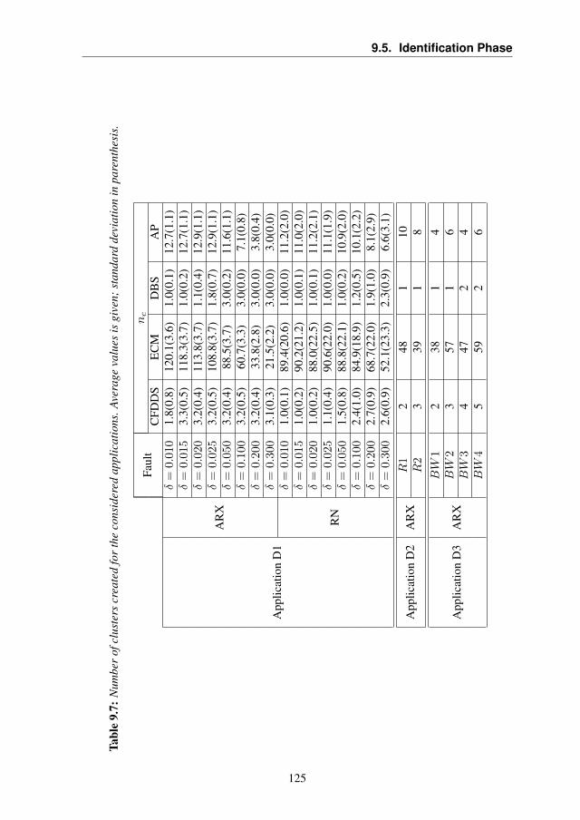
9.5. Identification Phase
Tabl
e9.
7:N
umbe
rof
clus
ters
crea
ted
for
the
cons
ider
edap
plic
atio
ns.A
vera
geva
lues
isgi
ven;
stan
dard
devi
atio
nin
pare
nthe
sis.
Faul
tnc
CFD
DS
EC
MD
BS
AP
App
licat
ion
D1
AR
X
δ=
0.010
1.8(
0.8)
120.
1(3.
6)1.
0(0.
1)12
.7(1
.1)
δ=
0.015
3.3(
0.5)
118.
3(3.
7)1.
0(0.
2)12
.7(1
.1)
δ=
0.020
3.2(
0.4)
113.
8(3.
7)1.
1(0.
4)12
.9(1
.1)
δ=
0.025
3.2(
0.5)
108.
8(3.
7)1.
8(0.
7)12
.9(1
.1)
δ=
0.050
3.2(
0.4)
88.5
(3.7
)3.
0(0.
2)11
.6(1
.1)
δ=
0.100
3.2(
0.5)
60.7
(3.3
)3.
0(0.
0)7.
1(0.
8)δ
=0.
200
3.2(
0.4)
33.8
(2.8
)3.
0(0.
0)3.
8(0.
4)δ
=0.
300
3.1(
0.3)
21.5
(2.2
)3.
0(0.
0)3.
0(0.
0)
RN
δ=
0.010
1.0(
0.1)
89.4
(20.
6)1.
0(0.
0)11
.2(2
.0)
δ=
0.015
1.0(
0.2)
90.2
(21.
2)1.
0(0.
1)11
.0(2
.0)
δ=
0.020
1.0(
0.2)
88.0
(22.
5)1.
0(0.
1)11
.2(2
.1)
δ=
0.025
1.1(
0.4)
90.6
(22.
0)1.
0(0.
0)11
.1(1
.9)
δ=
0.050
1.5(
0.8)
88.8
(22.
1)1.
0(0.
2)10
.9(2
.0)
δ=
0.100
2.4(
1.0)
84.9
(18.
9)1.
2(0.
5)10
.1(2
.2)
δ=
0.200
2.7(
0.9)
68.7
(22.
0)1.
9(1.
0)8.
1(2.
9)δ
=0.
300
2.6(
0.9)
52.1
(23.
3)2.
3(0.
9)6.
6(3.
1)
App
licat
ion
D2
AR
XR
12
481
10R
23
391
8
App
licat
ion
D3
AR
X
BW
12
381
4BW
23
571
6BW
34
472
4BW
45
592
6
125

Chapter 9. Experimental Results
Results Results are presented in Table 9.7 and Table 9.8. In particular,Table 9.7 shows the number of created clusters nc for the considered algo-rithms, model hierarchies and fault magnitudes. As expected, the ability tocreate the correct number of clusters increases with the magnitude of δ (astrong fault is easily identified). Interestingly, the proposed CFDDS basedon ARX modeling is able to correctly create three clusters even with verylow fault magnitudes (e.g., δ = 0.015). ECM creates an excessive num-ber of clusters making this algorithm not useful in this application. Thereason of this behaviour resides in the incorrect setting of Dthr [35]. Un-fortunately, as explained above, it is hard to set this parameter for fault di-agnosis purposes, since it is related to the number of clusters to be created,which is obviously unknown a priori. Interestingly, both DBSCAN andAP with ARX are able to create the correct number of clusters, for large δmagnitudes, i.e., δ ≥ 0.05 and δ ≥ 0.3, respectively. Despite the evolvingapproach, the proposed CFDDS with ARX is more effective in creating thecorrect number of clusters once compared with non-evolving algorithmssuch as the DBSCAN and the AP even for small δs. The rationale behindthis refers to the fact that the proposed CFDDS is able to simultaneouslyconsider both temporal and spatial dependencies among parameter vectors.
RNs provide lower performance than ARX. The reason of this behaviourcan be associated to the fact that the performance of RNs is highly influ-enced by the choice of the random network topology. In fact, training thenetwork topology is entirely based on nominal state samples. This leadsto a RN modeling the nominal state, but does not necessarily guaranteethe ability to identify new states during the operational life. However, theability to create the correct number of clusters increases with δ and the pro-posed CFDDS with RN is able to identify the correct number of faults withmagnitude δ ≥ 0.2.
126
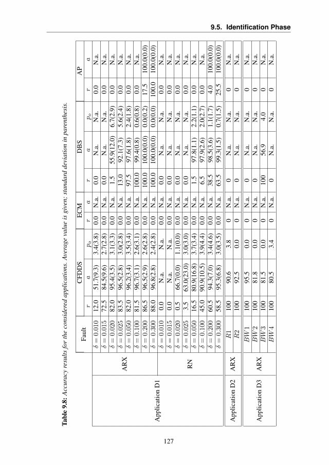
9.5. Identification Phase
Tabl
e9.
8:A
ccur
acy
resu
ltsfo
rth
eco
nsid
ered
appl
icat
ions
.Ave
rage
valu
eis
give
n;st
anda
rdde
viat
ion
inpa
rent
hesi
s.
Faul
tC
FDD
SE
CM
DB
SA
Pr
apo
ra
ra
po
ra
App
licat
ion
D1
AR
X
δ=
0.010
12.0
51.7
(9.3
)3.
4(3.
8)0.
0N
.a.
0.0
N.a
.N
.a.
0.0
N.a
.δ
=0.
015
72.5
84.5
(9.6
)2.
7(2.
8)0.
0N
.a.
0.0
N.a
.N
.a.
0.0
N.a
.δ
=0.
020
82.0
95.4
(3.5
)3.
1(3.
3)0.
0N
.a.
1.5
55.9
(12.
0)6.
7(2.
9)0.
0N
.a.
δ=
0.025
83.5
96.5
(2.8
)3.
0(2.
8)0.
0N
.a.
13.0
92.1
(7.3
)5.
6(2.
4)0.
0N
.a.
δ=
0.050
82.0
96.2
(3.4
)3.
5(3.
4)0.
0N
.a.
97.5
97.6
(1.8
)2.
4(1.
8)0.
0N
.a.
δ=
0.100
81.5
96.7
(3.1
)2.
6(3.
1)0.
0N
.a.
100.
099
.4(0
.8)
0.6(
0.8)
0.0
N.a
.δ
=0.
200
86.5
96.5
(2.9
)2.
6(2.
8)0.
0N
.a.
100.
010
0.0(
0.0)
0.0(
0.2)
17.5
100.
0(0.
0)δ
=0.
300
88.0
96.8
(2.8
)2.
4(2.
8)0.
0N
.a.
100.
010
0.0(
0.0)
0.0(
0.0)
100.
010
0.0(
0.0)
RN
δ=
0.010
0.0
N.a
.N
.a.
0.0
N.a
.0.
0N
.a.
N.a
.0.
0N
.a.
δ=
0.015
0.0
N.a
.N
.a.
0.0
N.a
.0.
0N
.a.
N.a
.0.
0N
.a.
δ=
0.020
0.5
66.7
(0.0
)1.
1(0.
0)0.
0N
.a.
0.0
N.a
.N
.a.
0.0
N.a
.δ
=0.
025
3.5
63.0
(23.
0)3.
0(3.
0)0.
0N
.a.
0.0
N.a
.N
.a.
0.0
N.a
.δ
=0.
050
16.5
80.9
(16.
8)3.
7(3.
4)0.
0N
.a.
1.5
97.8
(1.1
)2.
2(1.
1)0.
0N
.a.
δ=
0.100
45.0
90.9
(10.
5)3.
9(4.
4)0.
0N
.a.
6.5
97.9
(2.6
)2.
0(2.
7)0.
0N
.a.
δ=
0.200
60.5
94.3
(7.0
)3.
4(4.
6)0.
0N
.a.
38.5
98.5
(3.6
)1.
1(1.
7)4.
010
0.0(
0.0)
δ=
0.300
58.5
95.3
(6.8
)3.
0(3.
5)0.
0N
.a.
63.5
99.3
(1.5
)0.
7(1.
5)25
.510
0.0(
0.0)
App
licat
ion
D2
AR
XR
110
090
.63.
80
N.a
.0
N.a
.N
.a.
0N
.a.
R2
100
92.5
0.0
0N
.a.
0N
.a.
N.a
.0
N.a
.
App
licat
ion
D3
AR
X
BW
110
095
.50.
00
N.a
.0
N.a
.N
.a.
0N
.a.
BW
210
081
.80.
00
N.a
.0
N.a
.N
.a.
0N
.a.
BW
310
081
.50.
00
N.a
.10
056
.94.
00
N.a
.BW
410
080
.53.
40
N.a
.0
N.a
.N
.a.
0N
.a.
127

Chapter 9. Experimental Results
Then, in order to evaluate the ability to correctly identify the stateswhere the process operates over time, we focus only on those experimentsfor which the number of created clusters is correct. Table 9.8 shows r, aand p0 for ARX, RN and different fault magnitudes, when the number ofclusters created by the algorithm is correct (i.e., nc = 3 for ApplicationD1).
As expected, the proposed CFDDS improves its performance both interms of percentage of experiments which identified the correct number ofclusters r and in terms of the classification accuracy a as the magnitude ofthe fault increases. Interestingly, when δ < 0.015 the CFDDS with ARXreduces its effectiveness in the clustering (i.e., r = 12.0% and a = 51.7%)meaning that small fault magnitudes represent challenging situations forthe proposed approach. In our opinion, this behaviour is due to the fact thatthe real parameter vectors corresponding to faulty states with magnitudeδ ≤ 0.01 are included in the neighbourhood Rαs of probability 1 − αsinduced by the cluster corresponding to the nominal state, thus even theparameter vectors estimated from faulty data are associated by the proposedalgorithm to the nominal state cluster.
Furthermore, the analysis of p0 allows us to evaluate the effect of thechoice of the proposed CFDDS parameters on performance. More specifi-cally, the parameter αs controls the percentage of structural outliers of theCFDDS and this is particularly evident by looking at the values of po inTable 9.8 which are in line with what expected from the theory. On thecontrary, the percentage of outliers of DBSCAN decreases, when the faultmagnitude increases. This is reasonable since the method does not contem-plate a fixed percentage of structural outliers.
By inspecting accuracy a, we see that the CFDDS with ARX provideshigher performance than the one with RN in the small perturbation case(δ ≤ 0.025). As the magnitude δ increases, there is no strong evidencefor selecting a specific model family. Nevertheless, the standard devia-tion of the accuracy of ARX model is lower than the RN model one. Thisbehaviour is in line with the difficulties in selecting the RN topology fol-lowing the discussions given for Table 9.7.
As expected, non evolving clustering algorithms like DBSCAN or APprovide higher performance than the proposed CFDDS when δ = 0.3. Thisis reasonable since these algorithms work in an off-line way, by analyzingthe whole dataset at once. On the contrary, the proposed CFDDS providesbetter performance than DBSCAN and AP with small values of δ, making itsuitable to manage subtle and not evident faults. Even in this case, the rea-son of this behaviour resides in the ability of the method to exploit temporal
128

9.5. Identification Phase
dependencies among parameter vectors during the operational life (whilenot evolving algorithms do not exploit time dependencies in the clusteringphase). ECM was never able to correctly identify the number of clusters, inline with comments following Table 9.7.
0.0025 0.005 0.0075 0.01 0.025 0.05 0.075 0.1 0.25 0%
10%
20%
30%
40%
50%
60%
70%
80%
90%
100%
αs
ap
o
r
(a) Average accuracy a, outlier percentage po and percentage of exper-iments where the algorithm creates the correct number of clusters rare reported for the experiments where nc = 3.
0.0025 0.005 0.0075 0.01 0.025 0.05 0.075 0.1 0.25
2
2.5
3
3.5
4
4.5
αs
n c
n
c
True number of clusters
(b) Average number of cluster nc created with different values of αs
Figure 9.12: Robustness analysis result for αs
We also performed a robustness analysis to evaluate the effects of vari-ations of the main parameters of the proposed CFDDS, i.e., αs, αm, ηt andλ, on the considered figures of merit. In the considered scenario (Applica-tion D1), which is characterized by a stationary process affected by abrupt
129

Chapter 9. Experimental Results
changes, parameter αs revealed to be the most sensitive one and its be-haviour is deeply investigated in the sequel. Figures 9.12a and 9.12b showhow the figures of merit a, p0, r and nc vary with αs ranging in the inter-val [2.5 · 10−3; 2.5 · 10−1]. As expected, p0 increases with αs and this isquite obvious since we are creating clusters that are more and more com-pact. For the considered scenario, αs = 0.025 guarantees the highest valueof r. Interestingly, lower values of αs create a reduced number of clusters,while larger ones create an excessive number of clusters. This behaviouris evident by looking at the values of nc in Figure 9.12b. The behaviourof the classification accuracy a is particularly interesting: small values ofαs create very large clusters, hence possibly misclassifying estimated pa-rameter vectors that belong to a different state (e.g., a faulty one). On thecontrary, large values of αs create very small clusters, hence generatingmany outliers (and this is evident by looking at the behaviour of p0 whenαs increases). Due to the fact that αs is closely related to the confidence ofincluding a parameter vector in a cluster (i.e., 1−αs), reasonable values forthis parameters belong to the interval 0.01 ≤ αs ≤ 0.1.
9.5.2 Application D2: Rialba Dataset
Experimental Setting The dataset here considered, consists in 35652 sam-ples coming from two clinometers. In this application, the first M = 14260samples have been used to train the proposed CFDDS. Two different faultyscenarios have been considered:
R1
An abrupt additive fault affecting the measurements of theclinometer, regarded as output, is injected in sampleinterval [17468, 24956]. The magnitude of the additivefault is −20% of the signal dynamics
R2
The first 24956 samples are equal to the R1 case. Then, adegradation fault is injected in the same clinometer insample interval [28164, 35652]. The degradation faultconsists in an additive Gaussian noise with zero mean andstandard deviation equal to 30% of the signal one
As a model hierarchy family we here considered the ARX one. Experi-mental results on this application are particularly interesting since data arecoming from a real monitoring system.
Results In Table 9.8 the value of r is either 0 or 100, since here we areconsidering a single experiment. The proposed CFDDS accuracy in R1
130

9.5. Identification Phase
and R2, presented in Table 9.8, are similar (i.e., 90.6% in R1 and 92.5% inR2), showing that we are able to deal effectively with multiple faults.
By looking at Table 9.7, we see that the number of states of the processis correctly recognized by the proposed CFDDS in both scenarios whereasother methods are never able to create the correct number of clusters. Theseresults are in line with the synthetic scenario (Application D1): AP andECM are creating more clusters than necessary and DBSCAN is creating asingle cluster.
9.5.3 Application D3: Barcelona Water Distribution Network SystemDataset
Experimental Setting In this third scenario, we are considering a MISO ARXmodel for the estimation of the parameter vectors, where as output weconsidered the value of the flow in the iOrioles pump and as inputthe values of the flow in pumps near to it, i.e., iStamClmCervello,iCesalpina1, iCesalpina2 and . Four different scenarios have beenconsidered. The proposed CFDDS has been trained on the first M = 8736samples (representing one year of observations in the BWNDS simulator);as a reference model we consider the ARX.
Four different faulty scenarios have been considered:
131
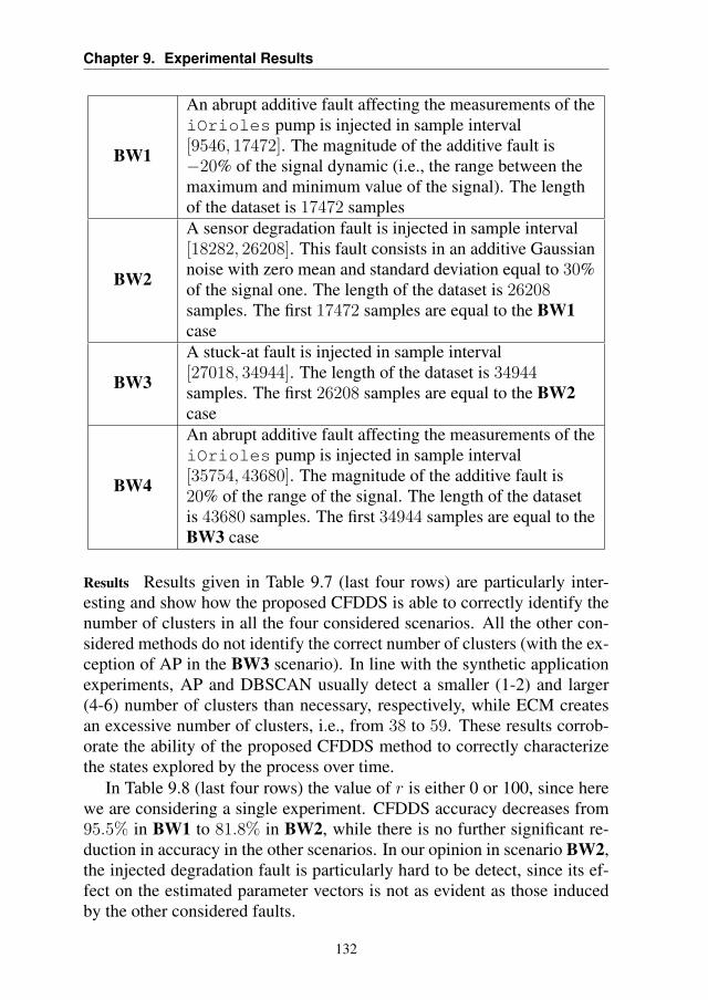
Chapter 9. Experimental Results
BW1
An abrupt additive fault affecting the measurements of theiOrioles pump is injected in sample interval[9546, 17472]. The magnitude of the additive fault is−20% of the signal dynamic (i.e., the range between themaximum and minimum value of the signal). The lengthof the dataset is 17472 samples
BW2
A sensor degradation fault is injected in sample interval[18282, 26208]. This fault consists in an additive Gaussiannoise with zero mean and standard deviation equal to 30%of the signal one. The length of the dataset is 26208samples. The first 17472 samples are equal to the BW1case
BW3
A stuck-at fault is injected in sample interval[27018, 34944]. The length of the dataset is 34944samples. The first 26208 samples are equal to the BW2case
BW4
An abrupt additive fault affecting the measurements of theiOrioles pump is injected in sample interval[35754, 43680]. The magnitude of the additive fault is20% of the range of the signal. The length of the datasetis 43680 samples. The first 34944 samples are equal to theBW3 case
Results Results given in Table 9.7 (last four rows) are particularly inter-esting and show how the proposed CFDDS is able to correctly identify thenumber of clusters in all the four considered scenarios. All the other con-sidered methods do not identify the correct number of clusters (with the ex-ception of AP in the BW3 scenario). In line with the synthetic applicationexperiments, AP and DBSCAN usually detect a smaller (1-2) and larger(4-6) number of clusters than necessary, respectively, while ECM createsan excessive number of clusters, i.e., from 38 to 59. These results corrob-orate the ability of the proposed CFDDS method to correctly characterizethe states explored by the process over time.
In Table 9.8 (last four rows) the value of r is either 0 or 100, since herewe are considering a single experiment. CFDDS accuracy decreases from95.5% in BW1 to 81.8% in BW2, while there is no further significant re-duction in accuracy in the other scenarios. In our opinion in scenario BW2,the injected degradation fault is particularly hard to be detect, since its ef-fect on the estimated parameter vectors is not as evident as those inducedby the other considered faults.
132

9.6. General Remarks
We emphasize that, to ease the comparison, R1 and R2 in the Rialbadataset (Application D2) correspond to BW1 and BW2 in the BWNDS one(Application D3), respectively. With respect to the BWNDS application,in the Rialba one we do not have a decrease in performance as the degra-dation fault appears, suggesting that, in this application, the effect of thedegradation fault is more easy to be perceived by the proposed CFDDS.
9.6 General Remarks
The experimental campaign we presented above provides evidence for theabilities of the proposed CFDDS to perform the fault detection and diag-nosis tasks (graph learning, detection, isolation and identification) on theconsidered sensor network scenarios. At first, it was shown that an effec-tive learning of the dependency graph improves the performance in detect-ing faults or changes in the environment. Then, we showed that the useof an ensemble of HMM-CDTs improves the detection performance on asingle HMM-CDT. The isolation phase of the proposed CFDDS is able toprovided results which are most of the times comparable with those ob-tained with the PTPR approach. Interestingly, the proposed solution doesnot require any a priori information about the system, while the latter onerequires the analytic model for the data generating process. Finally, resultson the identification phase of the proposed CFDDS provided evidence forits ability to characterize the nominal state and to identify and learn newfaulty states.
133


CHAPTER10Concluding Remarks
Sensor networks are well-known technological solutions to monitor com-plex systems or environmental phenomena. These sensing infrastructureswork in harsh environmental conditions, which might induce degradationof the mechanical parts of the sensors and malfunctions in the embeddedelectronic boards. Hence, an effective fault detection and diagnosis activ-ity is required. Since traditional methods for fault detection and diagnosisgenerally require the knowledge of a priori information about the data gen-erating process or the faults, in the last few years a novel generation of faultdetection and diagnosis systems has been developed. These systems, thatare usually addressed as “cognitive”, are able to characterize the nominalconditions of a system and learn the faults, by exploiting functional rela-tionships present in the acquired data.
In this dissertation we propose a novel Cognitive Fault Detection and Di-agnosis System (CFDDS), which operates in the sensor network scenario.This system is able to automatically characterize the nominal state of theprocess inspected by the network, by relying on the spatial and temporal re-dundancies provided by data gathered by the sensor network, and to detectthe occurrence and characterize faults, as they appear. This method doesnot require a priori information about either the process in nominal condi-
135
Chapter 10. Concluding Remarks
tions, or the signature of the occurring faults (fault dictionary), but relieson a dataset composed of fault-free data that are used to characterize thenominal conditions of the data generating process.
The proposed CFDDS is able to learn the dependency graph correspond-ing to the functional dependencies existing among data by relying on astatistical test based on the Granger causality. This procedure does not con-stitute a diagnostic phase per se, but represents the basis of all the otherdetection and diagnosis phases.
The detection phase is carried out by means of a HMM modeling ofthe parameter vectors estimated on data coming from the nominal state ofthe functional relationships included in the previously learned dependencygraph. A change in a functional relationship is detected by inspecting theloglikelihood provided by the HMM. An ensemble method for HMM-CDThas been proposed to further improve the detection performance.
Once the fault has been detected, the joint use of a partition of thelearned dependency graph and the statistical modeling given by the HMMis used to discriminate between a change in the data generating process or afault. In the case a fault occurred, the isolation phase is able also to identifythe location where it appeared.
The proposed CFDDS is able to identify different faults by means of anovel evolving clustering algorithm, which is able to learn the characteri-zation of the nominal state of the process in the parameter space, i.e., bycreating a cluster of estimated parameter vectors. Newly estimated param-eter vectors are assigned to either the nominal cluster or to one of the faultyones. The method, starting from an empty fault dictionary, is also able tocharacterize new faulty states in an on-line manner.
The CFDDS performance has been tested on a synthetically generatednonlinear dataset and on two real testbed scenarios, i.e., data coming from arock collapse and landslide forecasting system and from a system monitor-ing a water distribution network. The chosen real benchmarks are valuableexamples of systems where the need for a flexible and reliable frameworkfor fault detection and diagnosis is of paramount importance. In the formerapplication the data generating process is not known, thus a priori informa-tion about the nominal state of the process is missing. Moreover, a directinspection of the sensors is far from being trivial. In the latter system, thedifficulty in obtaining a precise modeling of the whole network, as well asthe difficulty in accessing the possibly faulty components (e.g., pipes andtanks) would benefit from a system which is able to detect and diagnosechanges and faults by relying solely on the inspection of the data comingfrom sensors. By considering the performance of the different phases (i.e.,
136

10.1. Future Perspectives
dependency graph learning, detection, isolation and identification) of theproposed CFDDS one at a time we showed that it outperforms the stateof the art methods for fault detection and diagnosis in the sensor networkscenario, thus providing a complete and useful tool for real world scenarios.
10.1 Future Perspectives
Up to present times, the study of the field of fault detection and diagnosisin the sensor network scenario is far from being completed. For instance,in the last few years the problem of handling huge amount of information(big data) has been raising interest in the scientific and industrial fields.In the sensor network scenario we could consider two different situationswhere this problem is relevant: when the sensor network is characterizedby a very high number of sensors and when it is not possible to store all thedata gathered from the network over time (e.g., due to a very high samplingrate). In the former case, the study of appropriate techniques for handlingdependency graphs with a high amount of nodes is required, for instanceby considering portions of the network one at a time and then combiningthe decisions taken over each subset of the partition. Another viable solu-tion is to apply dimensionality reduction techniques, where the goal is notto discard the redundant information provided by the network, but to use itfor fault diagnosis purposes. In the latter case, we should implement algo-rithms which are able to process data as they come (one pass algorithms)and update the knowledge base incrementally and in an evolving manner.The proposed CFDDS, in its evolving clustering identification phase, isable to address these issues, but the learning of the HMM in the detectionphase has not been designed to take into account this scenario.
In this dissertation we did not take into account the accommodation ofoccurred faults. It could be interesting to be able to deal with faults bymaintaining an acceptable level of service provided by the application thatbases its decision on the sensor network data, even if a sensor is no morereliable. For instance, one could consider systems which are able to eitherreconstruct the signal that a faulty sensor would have provided (virtual sen-sor) or to exclude the faulty sensor from the decision making algorithm.In the former case efficient and reliable mechanisms for the reconstructionof the signal should be considered, for instance by exploiting data comingfrom other sensors and from past observations of the faulty sensor itself. Inthe latter case, mechanisms which are able to reconfigure both the applica-tion and the fault detection and diagnosis system should be designed.
137


List of Figures
1.1 General scheme of a monitoring system . . . . . . . . . . . 41.2 Fault detection taxonomy . . . . . . . . . . . . . . . . . . . 61.3 Fault diagnosis taxonomy . . . . . . . . . . . . . . . . . . . 61.4 Generic fault detection scheme . . . . . . . . . . . . . . . . 71.5 Data-driven scheme for fault detection . . . . . . . . . . . . 81.6 Signal-based scheme for fault detection . . . . . . . . . . . 91.7 Process-based scheme for fault detection . . . . . . . . . . . 10
2.1 Specification of the considered faults . . . . . . . . . . . . . 242.2 Fault monitoring system . . . . . . . . . . . . . . . . . . . 252.3 Fault affecting the mounting of units on the rock face . . . . 272.4 Thermal drift affecting a MEMS tiltmeter . . . . . . . . . . 282.5 A low-probability intermittent fault at software level . . . . 29
3.1 General architecture of the proposed CFDDS . . . . . . . . 353.2 Example of dependency graph . . . . . . . . . . . . . . . . 37
4.1 Dependency graph learning phase of the proposed CFDDS . 484.2 Example of dependency graph learning phase . . . . . . . . 53
5.1 Proposed scheme for fault detection . . . . . . . . . . . . . 565.2 Mahalanobis-based detection phase of the proposed CFDDS 575.3 Example of Mahalanobis-based detection . . . . . . . . . . 595.4 Example of HMM . . . . . . . . . . . . . . . . . . . . . . 605.5 HMM-CDT detection phase . . . . . . . . . . . . . . . . . 61
139

List of Figures
5.6 Detection phase of the proposed CFDDS . . . . . . . . . . 655.7 Example of EHMM-CDT . . . . . . . . . . . . . . . . . . . 68
6.1 Isolation phase of the proposed CFDDS . . . . . . . . . . . 726.2 Examples of dependency graphs . . . . . . . . . . . . . . . 746.3 Example of the proposed cognitive isolation . . . . . . . . . 75
7.1 Identification phase of the proposed CFDDS . . . . . . . . . 807.2 Example of the identification phase in the proposed CFDDS 847.3 Example of different incipient faults . . . . . . . . . . . . . 92
9.1 Example of generation of the dependency graph . . . . . . . 989.2 The measurements acquired from two clinometers . . . . . . 999.3 Scheme for the BWNDS . . . . . . . . . . . . . . . . . . . 1009.4 Precision in the linear case . . . . . . . . . . . . . . . . . . 1039.5 Precision in the sinusoidal case . . . . . . . . . . . . . . . . 1039.6 Recall in the linear case . . . . . . . . . . . . . . . . . . . . 1049.7 Recall in the sinusoidal case . . . . . . . . . . . . . . . . . 1049.8 Box-plot for the best correlation . . . . . . . . . . . . . . . 1059.9 Results for the detection phase on Application D1 . . . . . . 1119.10 iOrioles subsystem . . . . . . . . . . . . . . . . . . . . . . 1159.11 Scheme of the iOrioles dependency graph . . . . . . . . . . 1169.12 Robustness analysis result for αs . . . . . . . . . . . . . . . 129
140
List of Tables
1.1 Relevant approaches in Cognitive FDDS . . . . . . . . . . . 13
9.1 Detection results for Application D1 . . . . . . . . . . . . . 1069.2 Detection results for Application D2: the numeric values are
detection delays DD for different dependency graph learn-ing algorithms, while FP and FN stands for false positiveand false negative detections, respectively. . . . . . . . . . . 108
9.3 Detection results for the single and ensemble HMM-CDTapproaches . . . . . . . . . . . . . . . . . . . . . . . . . . 112
9.5 Detection and isolation results for the Application D3 . . . . 1199.6 Parameters of the proposed CFDDS . . . . . . . . . . . . . 1239.7 Number of clusters created for the considered applications . 1259.8 Accuracy results for the considered applications . . . . . . . 127
141


Bibliography
[1] isense project website: http://www.i-sense.org/, mar 2014.
[2] matlab cognitive fault diagnosis system toolbox and dataset: http://home.deib.polimi.it/trovo/downloads, jan 2015.
[3] Raj K Aggarwal, QY Xuan, Allan T Johns, Furong Li, and Allen Bennett. A novel approach tofault diagnosis in multicircuit transmission lines using fuzzy artmap neural networks. NeuralNetworks, IEEE Transactions on, 10(5):1214–1221, 1999.
[4] Richard A Ajayi, Joseph Friedman, and Seyed M Mehdian. On the relationship between stockreturns and exchange rates: tests of granger causality. Global Finance Journal, 9(2):241–251,1999.
[5] C. Alippi, R. Camplani, C. Galperti, A. Marullo, and M. Roveri. An hybrid wireless-wiredmonitoring system for real-time rock collapse forecasting. In Mobile Adhoc and Sensor Sys-tems (MASS), 2010 IEEE 7th International Conference on, pages 224–231. IEEE, 2010.
[6] C. Alippi, R. Camplani, C. Galperti, A. Marullo, and M. Roveri. A high-frequency samplingmonitoring system for environmental and structural applications. ACM Transactions on SensorNetworks (TOSN), 9(4):41, 2013.
[7] C. Alippi, S. Ntalampiras, and M. Roveri. An hmm-based change detection method for intelli-gent embedded sensors. In Neural Networks (IJCNN), The 2012 International Joint Conferenceon, pages 1–7. IEEE, 2012.
[8] C. Alippi, S. Ntalampiras, and M. Roveri. A cognitive fault diagnosis system for distributedsensor networks. Neural Networks and Learning Systems, IEEE Transactions on, 24(8):1213– 1226, 2013.
[9] C. Alippi, S. Ntalampiras, and M. Roveri. Model ensemble for an effective on-line reconstruc-tion of missing data in sensor networks. In Neural Networks (IJCNN), The 2013 InternationalJoint Conference on, pages 1–6. IEEE, 2013.
143

Bibliography
[10] C. Alippi, M. Roveri, and F. Trovò. A “learning from models” cognitive fault diagnosis system.In Artificial Neural Networks and Machine Learning–ICANN 2012, pages 305–313. Springer,2012.
[11] C. Alippi, M. Roveri, and F. Trovò. A self-building and cluster-based cognitive fault diagnosissystem for sensor networks. Neural Networks and Learning Systems, IEEE Transactions on,25(6):1021 – 1032, 2014.
[12] Cesare Alippi. Intelligence for Embedded Systems. Springer, 2014.
[13] Cesare Alippi, Giacomo Boracchi, and Manuel Roveri. On-line reconstruction of missing datain sensor/actuator networks by exploiting temporal and spatial redundancy. In Neural Networks(IJCNN), The 2012 International Joint Conference on, pages 1–8. IEEE, 2012.
[14] Cesare Alippi, Stavros Ntalampiras, and Manuel Roveri. Model ensemble for an effectiveon-line reconstruction of missing data in sensor networks. In IJCNN, pages 1–6, 2013.
[15] Cesare Alippi, Manuel Roveri, and Francesco Trovò. Learning causal dependencies to detectand diagnose faults in sensor networks. In Computational Intelligence, Intelligent EmbeddedSystems (IES), 2014 IEEE Symposium on. IEEE, 2014 (to appear).
[16] T.W. Anderson. The statistical analysis of time series, volume 19. John Wiley & Sons, 2011.
[17] P.P. Angelov, P. Angelov, D.P. Filev, and N. Kasabov. Evolving intelligent systems: methodol-ogy and applications, volume 12. Wiley-IEEE Press, 2010.
[18] L. Barnett and A.K. Seth. The mvgc multivariate granger causality toolbox: A new approachto granger-causal inference. Journal of neuroscience methods, 223:50–68, 2014.
[19] A.B. Barrett, L. Barnett, and A.K. Seth. Multivariate granger causality and generalized vari-ance. Physical Review E, 81(4):041907, 2010.
[20] Adam B Barrett, Michael Murphy, Marie-Aurélie Bruno, Quentin Noirhomme, Mélanie Boly,Steven Laureys, and Anil K Seth. Granger causality analysis of steady-state electroencephalo-graphic signals during propofol-induced anaesthesia. PloS one, 7(1):e29072, 2012.
[21] Michèle Basseville, Igor V Nikiforov, et al. Detection of abrupt changes: theory and applica-tion, volume 104. Prentice Hall Englewood Cliffs, 1993.
[22] L.E. Baum, T. Petrie, G. Soules, and N. Weiss. A maximization technique occurring in thestatistical analysis of probabilistic functions of markov chains. The annals of mathematicalstatistics, 41:164–171, 1970.
[23] Avrim Blum. Random projection, margins, kernels, and feature-selection. In Subspace, LatentStructure and Feature Selection, pages 52–68. Springer, 2006.
[24] Frey Brendan J. and Dueck Delbert. Clustering by passing messages between data points.Science, 315:972–976, 2007.
[25] E. Caini, V. Puig Cayuela, G. Cembrano Gennari, et al. Development of a simulation environ-ment for water drinking networks: Application to the validation of a centralized mpc controllerfor the barcelona case study. Technical report, Universitat Politècnica de Catalunya, 2010.
[26] H. Chen, P. Tino, A. Rodan, and Xin Yao. Learning in the model space for cognitive faultdiagnosis. Neural Networks and Learning Systems, IEEE Transactions on, 25(1):124–136, Jan2014.
144

Bibliography
[27] J.B. Comly, P.P. Bonissone, and M.E. Dausch. Fuzzy logic for fault diagnosis. GE Research &Development Center, 1990.
[28] M.A. Cuguero, J. Quevedo, C. Alippi, M. Roveri, V. Puig, D. Garcia, and F. Trovò. Faultdiagnosis in drinking water transport networks: Physical/temporal parity relations vs. hmm-based cognitive method. Journal of Hydroinformatics, 2014 (submitted).
[29] R.I.A. Davis and B.C. Lovell. Comparing and evaluating hmm ensemble training algorithmsusing train and test and condition number criteria. Formal Pattern Analysis & Applications,6(4):327–335, 2004.
[30] M.A. Demetriou and M.M. Polycarpou. Incipient fault diagnosis of dynamical systems usingonline approximators. Automatic Control, IEEE Transactions on, 43(11):1612–1617, 1998.
[31] A.P. Dempster et al. Maximum likelihood from incomplete data via the em algorithm. Journalof the Royal statistical Society, 39(1):1–38, 1977.
[32] Gopikrishna Deshpande, Stephan LaConte, George Andrew James, Scott Peltier, and XiaopingHu. Multivariate granger causality analysis of fmri data. Human brain mapping, 30(4):1361–1373, 2009.
[33] Y. Ding, P. Kim, D. Ceglarek, and J. Jin. Optimal sensor distribution for variation diagnosis inmultistation assembly processes. Robotics and Automation, IEEE Transactions on, 19(4):543–556, 2003.
[34] R.J. Elliott, L. Aggoun, and J.B. Moore. Hidden Markov Models. Springer, 1995.
[35] Martin Ester, Hans-Peter Kriegel, Jörg Sander, and Xiaowei Xu. A density-based algorithmfor discovering clusters in large spatial databases with noise. In Proceedings of KDD. KDD,1996.
[36] J. Farrell, T. Berger, and BD Appleby. Using learning techniques to accommodate unantici-pated faults. Control Systems, IEEE, 13(3):40–49, 1993.
[37] J. Gertler. Fault detection and diagnosis in engineering systems. CRC, 1998.
[38] C.W.J. Granger. Investigating causal relations by econometric models and cross-spectral meth-ods. Econometrica: Journal of the Econometric Society, 27(3):424–438, July 1969.
[39] James Douglas Hamilton. Time series analysis, volume 2. Princeton university press Princeton,1994.
[40] J. Hardin and D.M. Rocke. Outlier detection in the multiple cluster setting using the minimumcovariance determinant estimator. Computational Statistics & Data Analysis, 44(4):625–638,2004.
[41] Wolfram Hesse, Eva Möller, Matthias Arnold, and Bärbel Schack. The use of time-variant eeggranger causality for inspecting directed interdependencies of neural assemblies. Journal ofneuroscience methods, 124(1):27–44, 2003.
[42] G.B. Huang, Q.Y. Zhu, and C.K. Siew. Extreme learning machine: theory and applications.Neurocomputing, 70(1):489–501, 2006.
[43] Yann-Chang Huang. Evolving neural nets for fault diagnosis of power transformers. PowerDelivery, IEEE Transactions on, 18(3):843–848, 2003.
145

Bibliography
[44] Yann-Chang Huang, Hong-Tzer Yang, and Ching-Lien Huang. Developing a new transformerfault diagnosis system through evolutionary fuzzy logic. Power Delivery, IEEE Transactionson, 12(2):761–767, 1997.
[45] R. Isermann. Fault-diagnosis systems: an introduction from fault detection to fault tolerance.Springer Verlag, 2006.
[46] R. Isermann. Fault-Diagnosis Applications: Model-Based Condition Monitoring: Actuators,drives, machinery, plants, sensors, and fault-tolerant systems. Springer, 2011.
[47] H. Jaeger. Tutorial on training recurrent neural networks, covering BPPT, RTRL, EKF and the“echo state network” approach. GMD-Forschungszentrum Informationstechnik, 2002.
[48] S. Jaiyen, C. Lursinsap, and S. Phimoltares. A very fast neural learning for classification usingonly new incoming datum. Neural Networks, IEEE Transactions on, 21(3):381–392, 2010.
[49] A. Joentgen, L. Mikenina, R. Weber, A. Zeugner, and H.J. Zimmermann. Automatic faultdetection in gearboxes by dynamic fuzzy data analysis. Fuzzy Sets and Systems, 105(1):123–132, 1999.
[50] R. A. Johnson and D. W. Wichern. Applied Multivariate Statistical Analysis. Prentice-Hall,Inc., Upper Saddle River, NJ, USA, 1988.
[51] Daniel Kaplan and Leon Glass. Understanding nonlinear dynamics, volume 19. Springer,1995.
[52] A. Khan and D. Ceglarek. Sensor optimization for fault diagnosis in multi-fixture assemblysystems with distributed sensing. TRANSACTIONS-AMERICAN SOCIETY OF MECHAN-ICAL ENGINEERS JOURNAL OF MANUFACTURING SCIENCE AND ENGINEERING,122(1):215–226, 2000.
[53] A.N. Kolmogorov. Sulla determinazione empirica di una legge di distribuzione. Giornaledell’Istituto Italiano degli Attuari, 4(1):83–91, 1933.
[54] A. Krogh and P. Sollich. Statistical mechanics of ensemble learning. Physical Review E,55(1):811, 1997.
[55] Anders Krogh, BjoÈrn Larsson, Gunnar Von Heijne, and Erik LL Sonnhammer. Predict-ing transmembrane protein topology with a hidden markov model: application to completegenomes. Journal of molecular biology, 305(3):567–580, 2001.
[56] M. Krysander and E. Frisk. Sensor placement for fault diagnosis. Systems, Man and Cyber-netics, Part A: Systems and Humans, IEEE Transactions on, 38(6):1398–1410, 2008.
[57] H.C. Kuo and H.K. Chang. A new symbiotic evolution-based fuzzy-neural approach to faultdiagnosis of marine propulsion systems. Engineering Applications of Artificial Intelligence,17(8):919–930, 2004.
[58] L. Ljung. Convergence analysis of parametric identification methods. Automatic Control, IEEETransactions on, 23(5):770–783, 1978.
[59] L. Ljung and P.E. Caines. Asymptotic normality of prediction error estimators for approximatesystem models. In Decision and Control including the 17th Symposium on Adaptive Processes,1978 IEEE Conference on, volume 17, pages 927–932. IEEE, 1978.
[60] Lennart Ljung. System identification. Wiley Online Library, 1999.
146

Bibliography
[61] Xinsheng Lou and Kenneth A Loparo. Bearing fault diagnosis based on wavelet transform andfuzzy inference. Mechanical systems and signal processing, 18(5):1077–1095, 2004.
[62] D.J.C. MacKay. Ensemble learning for hidden markov models. Technical report, Technicalreport, Cavendish Laboratory, University of Cambridge, 1997.
[63] P.C. Mahalanobis. On the generalized distance in statistics. In Proceedings of the NationalInstitute of Sciences of India, volume 2, pages 49–55. New Delhi, 1936.
[64] R. Naresh, V. Sharma, and M. Vashisth. An integrated neural fuzzy approach for fault diagnosisof transformers. Power Delivery, IEEE Transactions on, 23(4):2017–2024, 2008.
[65] O. Nasraoui and C. Rojas. Robust clustering for tracking noisy evolving data streams. In Proc.2006 SIAM Conf. on Data Mining (SDM 2006), pages 80–99, 2006.
[66] Philippe Pébay. Formulas for robust, one-pass parallel computation of covariance and arbitrary-order statistical moments. Technical report, Sandia National Laboratories, 09 2008.
[67] M.D. Penrose. Extremes for the minimal spanning tree on normally distributed points. Ad-vances in Applied Probability, 30(3):628–639, 1998.
[68] M.P. Perrone and L.N. Cooper. When networks disagree: Ensemble methods for hybrid neuralnetworks. Technical report, DTIC Document, 1992.
[69] J Quevedo, V Puig, G Cembrano, J Blanch, J Aguilar, D Saporta, G Benito, M Hedo, andA Molina. Validation and reconstruction of flow meter data in the barcelona water distributionnetwork. Control Engineering Practice, 18(6):640–651, 2010.
[70] Lawrence Rabiner and Biing-Hwang Juang. An introduction to hidden markov models. ASSPMagazine, IEEE, 3(1):4–16, 1986.
[71] A. Rosich, R. Sarrate, V. Puig, and T. Escobet. Efficient optimal sensor placement for model-based fdi using an incremental algorithm. In Decision and Control, 2007 46th IEEE Conferenceon, pages 2590–2595. IEEE, 2007.
[72] Manuel Roveri and Francesco Trovò. An ensemble of hmms for cognitive fault detection indistributed sensor networks. In Artificial Intelligence Applications and Innovations. Springer,2014 (to appear).
[73] R. Saunders and P. Laud. The mutltidimensional kolmogorov goodness-of-fit test. Biometrika,67(1):237–237, 1980.
[74] B. Schrauwen, D. Verstraeten, and J. Van Campenhout. An overview of reservoir computing:theory, applications and implementations. In Proceedings of the 15th European Symposium onArtificial Neural Networks. Citeseer, 2007.
[75] Gideon Schwarz. Estimating the dimension of a model. The annals of statistics, 6(2):461–464,1978.
[76] M.Ó. Searcóid. Metric spaces. Springer Verlag, 2006.
[77] Manjeevan Seera, Chee Peng Lim, Dahaman Ishak, and Harapajan Singh. Fault detection anddiagnosis of induction motors using motor current signature analysis and a hybrid fmm–cartmodel. Neural Networks and Learning Systems, IEEE Transactions on, 23(1):97–108, 2012.
147

Bibliography
[78] N. Smirnov. Table for estimating the goodness of fit of empirical distributions. The annals ofmathematical statistics, 19(2):279–281, 1948.
[79] Q. Song and N. Kasabov. Ecm-a novel on-line, evolving clustering method and its applications.In Proceedings of the fifth biannual conference on artificial neural networks and expert systems(ANNES2001), pages 87–92. Citeseer, 2001.
[80] A.B. Trunov and M.M. Polycarpou. Automated fault diagnosis in nonlinear multivariablesystems using a learning methodology. Neural Networks, IEEE Transactions on, 11(1):91–101, 2000.
[81] V. Venkatasubramanian, R. Rengaswamy, S.N. Kavuri, and K. Yin. A review of process faultdetection and diagnosis:: Part iii: Process history based methods. Computers & chemicalengineering, 27(3):327–346, 2003.
[82] J. Wichard and M. Ogorzalek. Time series prediction with ensemble models. In Proceedings ofInternational Joint Conference on Neural Networks (IJCNN 2004), pages 1625–1629. Citeseer,2004.
[83] C.W. Wu, J.L. Chen, and J.H. Wang. Self-organizing mountain method for clustering. InSystems, Man, and Cybernetics, 2001 IEEE International Conference on, volume 4, pages2434–2438. IEEE, 2001.
[84] Rui Xu and Don Wunsch. Clustering, volume 10. Wiley-IEEE Press, 2008.
[85] R.R. Yager and D.P. Filev. Approximate clustering via the mountain method. Systems, Manand Cybernetics, IEEE Transactions on, 24(8):1279–1284, 1994.
[86] B.S. Yang, T. Han, and Y.S. Kim. Integration of art-kohonen neural network and case-basedreasoning for intelligent fault diagnosis. Expert Systems with Applications, 26(3):387–395,2004.
[87] M.S. Yang and K.L. Wu. A similarity-based robust clustering method. Pattern Analysis andMachine Intelligence, IEEE Transactions on, 26(4):434–448, 2004.
[88] DL Yu, JB Gomm, and D Williams. Sensor fault diagnosis in a chemical process via rbf neuralnetworks. Control Engineering Practice, 7(1):49–55, 1999.
[89] G.P. Zhang. Time series forecasting using a hybrid arima and neural network model. Neuro-computing, 50:159–175, 2003.
[90] J Zhang and AJ Morris. On-line process fault diagnosis using fuzzy neural networks. Intelligentsystems engineering, 3(1):37–47, 1994.
[91] Z.H. Zhou. Ensemble methods: foundations and algorithms. CRC Press, 2012.
[92] I. Žliobaite. Combining similarity in time and space for training set formation under conceptdrift. Intelligent Data Analysis, 15(4):589–611, 2011.
148

Glossary
AIC Akaike Information Criterion. 94
ANFIS Adaptive Network-based Fuzzy Inference System. 14
ANN Artificial Neural Network. 9, 10
AP Affinity Propagation. 80, 121, 122, 126, 128, 131, 132
ARMAX Auto Regressive Moving Average eXogenous. 38
ART-KNN Adaptive Resonance Theory and Kohonen Neural Network. 14
ARX Auto Regressive eXogenous. 38, 94, 101, 109, 116, 122, 126, 128, 130, 131
BIC Bayesian Information Criterion. 122
BW Baum-Welch. 64, 65
BWNDS Barcelona Water Network Distribution System. 17, 100, 120, 131, 132
CDF Cumulative Distribution Function. 87
CDT Change Detection Test. 7, 73
CFDDS Cognitive Fault Detection and Diagnosis System. V, VI, 11, 16, 17, 20, 31, 33, 34, 35, 34,35, 36, 40, 42, 43, 44, 45, 44, 47, 49, 52, 55, 56, 57, 64, 67, 71, 73, 75, 77, 79, 81, 83, 85, 86,87, 88, 91, 93, 94, 95, 97, 108, 109, 114, 115, 116, 117, 120, 121, 122, 123, 126, 128, 129,130, 131, 132, 133, 135, 136, 137, 139, 140, 141
DB DataBase. 29
DBSCAN Density-Based Spatial Clustering of Applications with Noise. 80, 121, 122, 123, 126,128, 131, 132
ECM Evolving Cluster Method. 80, 121, 122, 123, 126, 128, 131, 132
EEG ElectroEncephaloGraphy. 49
EHMM-CDT Ensemble approach to Hidden Markov Model-Change Detection Test. 55, 64, 65,67, 69, 71, 79, 108, 110, 113, 140
149

Glossary
ELM Extreme Learning Machine. 38
FDDS Fault Detection and Diagnosis System. 3, 11, 13, 14, 15, 23, 30, 48, 141
fMRI functional Magnetic Resonance Imaging. 49
GMM Gaussian Mixture Model. 61, 62, 101, 109
HMM Hidden Markov Model. 15, 16, 43, 44, 56, 60, 61, 62, 63, 64, 65, 67, 71, 76, 93, 94, 95, 101,109, 116, 136, 137, 139
HMM-CDT Hidden Markov Model-Change Detection Test. VI, 15, 55, 60, 62, 63, 64, 65, 67, 69,100, 101, 105, 108, 109, 110, 112, 113, 116, 120, 133, 136, 139, 141
KNN K-Nearest Neighbours. 10
KS Kolmogorov-Smirnov. 44, 87, 88, 123
LM Levenberg-Marquardt. 41
LS Least Square. 9, 50, 109
LTI Linear Time Invariant. 16, 35, 38, 40, 56, 109
MEMS Micro Electro-Mechanical Systems. 28
MIMO Multiple Input Multiple Output. 41, 69
MISO Multiple Input Single Output. 38, 41, 131
ML Machine Learning. 14
MM Mountain Method. 88
MSE Mean Square Error. 94
PCA Principal Component Analysis. 9, 87
PTPR Physical/Temporal Parity Relations. 115, 116, 117, 120, 133
RBF Radial Basis Function. 14
RN Reservoir Network. 38, 122, 126, 128
RP Random Projection. 87
SIMO Single Input Multiple Output. 41
SISO Single Input Single Output. 101, 109
UMTS Universal Mobile Telecommunications System. 99
VAR Vector AutoRegressive. 49
150