a combined forecasting approach based on fuzzy soft sets

Journal of Computational and Applied Mathematics 228 (2009) 326–333

Contents lists available at ScienceDirect

Journal of Computational and AppliedMathematics

journal homepage: www.elsevier.com/locate/cam

A combined forecasting approach based on fuzzy soft setsZhi Xiao a, Ke Gong a,∗, Yan Zou ba School of Economics and Business Administration, Chongqing University, Chongqing 400044, PR Chinab College of Mathematics and Computer Science, Chongqing Normal University, Chongqing 400047, PR China

a r t i c l e i n f o

Article history:Received 6 August 2008

Keywords:Combined forecastingFuzzy soft setsSoft setsTime seriesRough sets

a b s t r a c t

Forecasting the export and import volume in international trade is the prerequisite of agovernment’s policy-making and guidance for a healthier international trade development.However, an individual forecast may not always perform satisfactorily, while combinationof forecasts may result in a better forecast than component forecasts. We believe thecomponent forecasts employed in combined forecasts are a description of the actual timeseries, which is fuzzy. This paper attempts to use forecasting accuracy as the criterion offuzzymembership function, and proposes a combined forecasting approach based on fuzzysoft sets. This paper also examines themethodwith data of international trade from1993 to2006 in the Chongqing Municipality of China and compares it with a combined forecastingapproach based on rough sets and each individual forecast. The experimental results showthat the combined approach provided in this paper improves the forecasting performanceof each individual forecast and is free from a rough sets approach’s restrictions as well. Itis a promising forecasting approach and a new application of soft sets theory.

© 2008 Elsevier B.V. All rights reserved.

1. Introduction

Forecasting the export and import volume in international trade is the prerequisite for a government to make a relevantpolicy and guide the international trade industry to develop healthier. However, the time series of export and importvolume is always fuzzy and nonlinear. The government concerns various categories of products which have their owndeveloping characteristics and trends and are related to local economic policies. For example, agricultural products havea very strong seasonal feature, and for products that the government gives vigorous support for have a characteristic ofrising exponentially, yet for those relatively mature types of products have very strong growth curve characteristic. Webelieve the time series of each type of product is uncertain or fuzzy. Therefore, using an individual specific method, such asthe Box–Jenkins model, the Holt–Winters model, exponential smoothing, artificial neural networks, regression over time,etc., to forecast export and import volume cannot always meet the government’s demand of high forecasting accuracy. Inthis case, there should be an expert systemor algorithm to solve the difficulty, which can identify and combine one or severalkinds of individual forecasting methods that are able to fit the time series better among the above. The process is to selectand combine individual forecasting methods among several ones by a set of linear weights, and the better the forecastingmethods fit the data, the greater is the weight.The concept of combining forecasts started with the seminal work of Bates et al. in [1]. They demonstrated that a suitable

linear combination of two forecastsmay result in a better forecast than the twooriginal ones. Dickinson [2] examined someofthe theoretical implications of combining forecasts using aminimumvariance criterion and proved that the error variance ofthe combining forecasts is no greater than that of any of the individual one.Makridakis andAndersen [3] introduced thewell-known M-competition, in which combination of forecasts from more than one model often lead to improved forecasting

∗ Corresponding author. Tel.: +86 13527563277.E-mail address: [email protected] (K. Gong).

0377-0427/$ – see front matter© 2008 Elsevier B.V. All rights reserved.doi:10.1016/j.cam.2008.09.033

http://www.elsevier.com/locate/cam

http://www.elsevier.com/locate/cam

mailto:[email protected]

http://dx.doi.org/10.1016/j.cam.2008.09.033

Z. Xiao et al. / Journal of Computational and Applied Mathematics 228 (2009) 326–333 327

performance. Throughout the years, many others have developed models to find the ‘‘optimal’’ combination of forecastsand it has been applied to many fields, such as business management, meteorology, economy, engineering, etc.Regarding combining forecasts, there are two ways to construct the weight of each individual forecast method. First,

much effort has been done to find the optimal fixedweights (FW) of individual forecasts tominimize thewithin-sample sumof squared forecast errors. Second, some researchers prefer changing the weights from time to time. Deutsch and Grangeret al. [4] used changing weights derived from switching regression models or from smooth transition regression models. Intheir empirical examples method, changed weight is not always well-performed compared with FW in terms of root meansquared errors (RMSE). Chan and Kingsman et al. [5] assessed the value of the improvement in forecasting performanceamong Simple Average, Fixed Weighting, Rolling WindowWeighting and Highest Weighting, and presented an applicationof combining forecasts in inventory forecast of a leading bank in Hong Kong. Zhong and Xiao [6] proposed a method ofdetermining the weighting coefficient based on rough sets theory, in which they used the significance of attributes in roughsets as the weighting criterion. Zhong and Xiao [7] are on the basis of [6]. They revised their work by introducing knowledgeentropy to compute the significance of attributes in rough sets. Prudêncio and Ludermir [8] employed a machine learningmethod to define the weight of each individual forecast and they implemented a multi-layer perceptron neural network(MLP) to combine two forecasts which have been brought into wide use. Zhang [9] have used a generalized autoregressiveconditional heteroskedasticity (GARCH) model to determine the optimal weights of component forecasts, and used themodel to forecast an actual time series of electronic products. The results shows that this weight-varying combinationalmethod performs better than other commonly used forecasting approaches which are based on single model selectioncriteria or fixed weights.We believe the individual methods in combined forecasts are a description of the actual time series, which are fuzzy.

Meanwhile, determining the optimalweights is a decision-making problem to find a vector, bywhich the combined forecastscan minimize the within-sample sum of squared forecasts errors. Therefore, we use the relative error of each individualforecast as the criterion to construct the membership function of fuzzy sets and make it reflect in a tabular form of fuzzysoft sets. This paper attempts to introduce the concept of fuzzy soft sets to construct the computing combined forecastalgorithm. Since the sample of export and import volume dataset is small and the application has to process millions ofkinds of time series, we choose fixed weight as the means of combination.Many practical problems in engineering, social, management, economics etc. are fuzzy, imprecise, and uncertain. Soft

sets theory is a newly-emerging tool to deal with uncertain problems. Molodtsov [10] initiated the concept of soft setstheory, in which the theory of probability, theory of fuzzy sets [11], and the interval mathematics were considered asmathematical tools for dealing with uncertainty, but all these theories have their own difficulties due to the inadequacyof the parameterization of the theory. He proposed the soft sets theory which may be free from such difficulties. On thebasis of Molodtsov, Maji and Biswas [12] defined equality of two soft sets, subset and super set of soft set, complement of asoft set, null soft set, and absolute soft set with examples. Also they defined soft binary operation such as AND, OR and theoperation of union, intersection and De Morgan’s law. Hacı Aktaş and Naim Çağman [13] introduced the basic propertiesof soft sets to the related concept of fuzzy sets as well as rough sets, and then they gave a definition of soft group andderive basic properties usingMolodtsov’s definition of the soft sets. Jun and Park. [14] proposed the notion of soft ideals andidealistic soft BCK/BCI-algebras, and gave several examples. They also provided the relations between soft BCK/BCI-algebrasand idealistic soft BCK/BCI-algebras and established intersection, union, AND operation, and OR operation of soft ideals andidealistic soft BCK/BCI-algebras.With the establishment of soft sets theory, its application has boomed in recent years. Maji and Roy [15] addressed

an application of soft sets theory in decision-making problems. Under Maji and Roy’s inspiration, Xiao and Li et al. [16]introduced soft sets theory into the research of business competitive capacity evaluation. Mushrif and Sengupta et al. [17]proposed a new algorithm for classification of the natural textures. Chen and Tsang et al. [18] presented a revised definitionof soft sets parameterization reduction, and compared with the related concept of attributes reduction in rough sets theory.Roy andMaji [19] use the notion of multi-observer and proposed a decision-making application of fuzzy soft sets. Moreover,an application example and its algorithm are also given. Although the algorithm is proved incorrect by Kong and Gaoet al. [20], the fuzzy soft sets andmulti-observer concept are valuable to successive researchers. Zou and Xiao [21] presenteda data analysis approach of soft sets under incomplete information and gave an application example in quality evaluationof information systems.The purpose of this paper is to introduce the soft sets theory for forecasting the export and import volume in international

trade.Wepropose a combined forecasting approach based on the fuzzy soft sets (CFFSS) and an algorithm is also addressed inthis paper. To prove the performance of the algorithm, we use the export dataset from 1993 to 2006 in Chongqing China andcompare themwith the combined forecasting approach based on the rough sets theory (CFRS) that was proposed in [7], andalso with the individual forecasts as well. The results shows the fuzzy soft sets approach outperforms the individual forecastin most situations and is almost equal to the rough sets approach but has a low time-consuming operation compared withthe rough sets approach. This is another new application of soft sets, which has enriched the soft sets theory application inreal life. The initial work can be found in [19], which proposed a fuzzy soft sets conception and multi-observer data. In fact,in future work, we may consider other factors that affect export and import. Moreover, the powerful parameterization andBoolean operations may help us to construct a more practical and complicated model.The rest of the paper is organized as follows. Section 2 introduces the basic principles of soft sets and fuzzy soft sets

and gives a simple example; for more details one can refer to [19]. Section 3 gives a description of the approach taken in

328 Z. Xiao et al. / Journal of Computational and Applied Mathematics 228 (2009) 326–333

the study and the algorithm. Section 4 exams the performance of the approach with the export datasets from 1993 to 2006in Chongqing China and compares the approach we provide with the rough sets approach proposed in [7], each individualforecast and some discussions. Finally Section 5 presents some conclusions from the research.

2. Preliminary

2.1. Soft sets

Definition 2.1 (See [10]). A pair (F , E) is called a soft set (over U) if and only if F is a mapping of E into the set of all subsetsof the set U .In other words, the soft set is a parameterized family of subsets of the set U . Every set F(ε)(ε ∈ E), from this family may

be considered as the set of ε-elements of the soft sets (F , E), or as the set of ε-approximate elements of the soft set.To illustrate this idea, let us consider the following example.

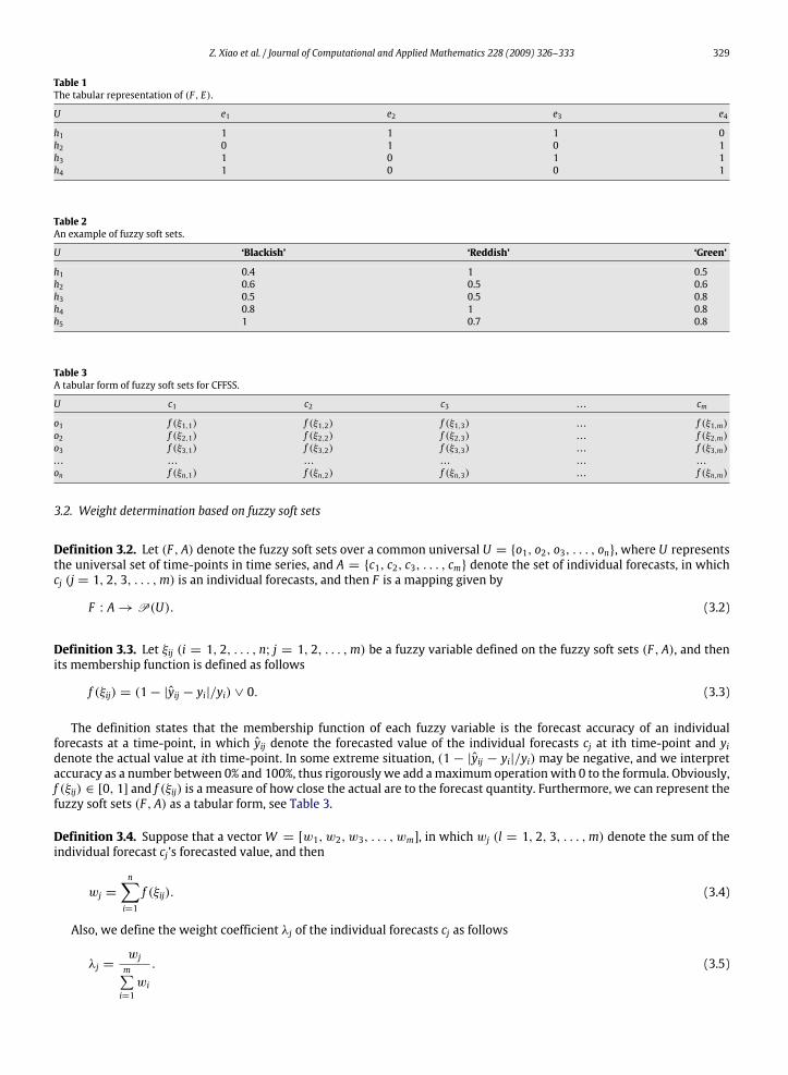
Example 2.1. Let universe U = {h1, h2, h3, h4} be a set of houses, a set of parameters E = {e1, e2, e3, e4} be a set of status ofhouses which stand for the parameters ‘‘beautiful’’, ‘‘cheap’’, ‘‘in green surroundings’’, and ‘‘in good location’’ respectively.Consider themapping F be amapping of E into the set of all subsets of the set U . Now consider a soft set (F , E) that describesthe ‘‘attractiveness of houses for purchase’’. According to the data collected, the soft set (F , E) is given by

{F , E} = {(e1, {h1, h3, h4}), (e2, {h1, h2}), (e3, {h1, h3}), (e4, {h2, h3, h4})}

where F(e1) = {h1, h3, h4}, F(e2) = {h1, h2}, F(e3) = {h1, h3} and F(e4) = {h2, h3, h4}.In order to store a soft set incomputer, a two-dimensional table is used to represent the soft set (F , E). Table 1 is the tabular form of the soft set (F , E).If hi ∈ F(ej), then hij = 1, otherwise hij = 0, where hij are the entries (see Table 1).

2.2. Fuzzy soft sets

The real world is inherently uncertain, imprecise and vague. Traditional mathematical tools cannot deal with suchproblems. The fuzzy sets theory is widely employed in such kinds of problems [11]. Maji and Biswas et al. [22] proposed thenotion of fuzzy soft sets and an example of decision-making was discussed in [19] as well.

Definition 2.2 (See [19,22]). LetP(U) denotes the set of all fuzzy sets of U . Let Ai ⊂ E.A pair (Fi, Ai) is called fuzzy soft sets over U , where Fi is a mapping given by

Fi : Ai → P(U). (2.1)

In view of the above discussions, we present an example below.

Example 2.2 (See [19]). Consider fuzzy soft sets (F , A) over the universal U = {h1, h2, h3, h4, h5}, in which U represents theset of house A = {blackish, reddish, green}, and

F (blackish) = {h1 /.4, h2 /.6, h3 /.5, h4 /.8, h5 /1},F (reddish) = {h1 /1, h2 /.5, h3 /.5, h4 /1, h5 /.7},F (green) = {h1 /.5, h2 /.6, h3 /.8, h4 /.8, h5 /.7}.

Also, we can express it in a tabular form in Table 2.

3. Combined forecasts model based on fuzzy soft sets

3.1. Combined forecasts model

Definition 3.1 (See [7]). Consider the time series forecasting problem,assume that y is an actual time series vector, andyt (t = 1, 2, . . . , n) is its time-point, c1, c2, . . . , cm denote m kinds of individual forecasts and let cjt (j = 1, 2, . . . ,m; t =1, 2, . . . , n) denote the ith forecasting value of individual forecasts at time-point t , and λj (j = 1, 2, . . . ,m) is the ith weightcoefficient of individual forecasts, yt denote the forecast value at time-point t , and then the combined forecastingmodel canbe written as follows

yt =m∑j=1

λjcjt . (3.1)

Clearly, if we have a known each weight coefficient λi = (i = 1, 2, . . . ,m) then we can forecast yt by the formula (3.1).


Table 1The tabular representation of (F , E).

U e1 e2 e3 e4

h1 1 1 1 0h2 0 1 0 1h3 1 0 1 1h4 1 0 0 1

Table 2An example of fuzzy soft sets.

U ‘Blackish’ ‘Reddish’ ‘Green’

h1 0.4 1 0.5h2 0.6 0.5 0.6h3 0.5 0.5 0.8h4 0.8 1 0.8h5 1 0.7 0.8

Table 3A tabular form of fuzzy soft sets for CFFSS.

U c1 c2 c3 . . . cm

o1 f (ξ1,1) f (ξ1,2) f (ξ1,3) . . . f (ξ1,m)o2 f (ξ2,1) f (ξ2,2) f (ξ2,3) . . . f (ξ2,m)o3 f (ξ3,1) f (ξ3,2) f (ξ3,3) . . . f (ξ3,m). . . . . . . . . . . . . . . . . .on f (ξn,1) f (ξn,2) f (ξn,3) . . . f (ξn,m)

3.2. Weight determination based on fuzzy soft sets

Definition 3.2. Let (F , A) denote the fuzzy soft sets over a common universal U = {o1, o2, o3, . . . , on}, where U representsthe universal set of time-points in time series, and A = {c1, c2, c3, . . . , cm} denote the set of individual forecasts, in whichcj (j = 1, 2, 3, . . . ,m) is an individual forecasts, and then F is a mapping given by

F : A→ P(U). (3.2)

Definition 3.3. Let ξij (i = 1, 2, . . . , n; j = 1, 2, . . . ,m) be a fuzzy variable defined on the fuzzy soft sets (F , A), and thenits membership function is defined as follows

f (ξij) = (1− |yij − yi|/yi) ∨ 0. (3.3)

The definition states that the membership function of each fuzzy variable is the forecast accuracy of an individualforecasts at a time-point, in which yij denote the forecasted value of the individual forecasts cj at ith time-point and yidenote the actual value at ith time-point. In some extreme situation, (1 − |yij − yi|/yi) may be negative, and we interpretaccuracy as a number between 0% and 100%, thus rigorously we add amaximum operationwith 0 to the formula. Obviously,f (ξij) ∈ [0, 1] and f (ξij) is a measure of how close the actual are to the forecast quantity. Furthermore, we can represent thefuzzy soft sets (F , A) as a tabular form, see Table 3.

Definition 3.4. Suppose that a vectorW = [w1, w2, w3, . . . , wm], in which wj (l = 1, 2, 3, . . . ,m) denote the sum of theindividual forecast cj’s forecasted value, and then

wj =

n∑i=1

f (ξij). (3.4)

Also, we define the weight coefficient λj of the individual forecasts cj as follows

λj =wjm∑i=1wi

. (3.5)


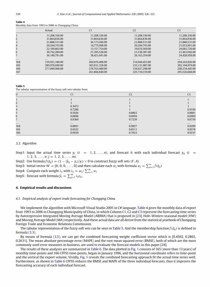
Table 4Monthly data from 1993 to 2006 in Chongqing China.

Actual C1 C2 C3

1 11,208,336.00 11,208,336.00 11,208,336.00 11,208,336.002 31,864,836.00 31,864,836.00 31,864,836.00 31,864,836.003 21,888,531.00 36,173,506.00 21,888,531.00 21,888,531.004 20,294,793.00 14,775,098.00 20,294,793.00 21,653,901.005 22,199,802.00 13,157,754.00 19,676,569.00 24,682,720.006 30,792,280.00 27,395,528.00 21,538,307.00 21,461,042.007 36,140,781.00 38,421,041.00 26,163,354.00 24,428,958.00. . . . . . . . . . . . . . .164 319,501,346.00 284,076,498.00 314,944,453.00 294,243,826.00165 289,978,690.00 303,831,328.00 333,131,987.00 302,194,979.00166 277,099,968.00 278,763,400.00 334,627,298.00 298,234,445.00167 . 261,866,840.00 325,734,319.00 295,526,668.00

Table 5The tabular representation of the fuzzy soft sets tabular form.

U C1 C2 C3

1 1 1 12 1 1 13 0.3473 1 14 0.7280 1 0.93305 0.5926 0.8863 0.88816 0.8896 0.6994 0.69697 0.9369 0.7239 0.6759. . . . . . . . . . . .164 0.8891 0.9857 0.9209165 0.9522 0.8511 0.9578166 0.9939 0.7923 0.9237

3.3. Algorithm

Step1: Input the actual time series yt (t = 1, 2, . . . , n), and forecast it with each individual forecast ytj (t =1, 2, 3, . . . , n; j = 1, 2, 3, . . . ,m)

Step2: Use formula f (ξij) = (1− |yij − yi|/yi) ∨ 0 to construct fuzzy soft sets (F , A)Step3: Initial vectorW = [0, 0, 0, . . . , 0] and then calculate eachwj with formulawj =

∑ni=1 f (ξij)

Step4: Compute each weight λj with λj = wj/∑mi=1wi

Step5: forecast with formula yt =∑mj=1 λjcjt .

4. Empirical results and discussions

4.1. Empirical analysis of export trade forecasting for Chongqing China

We implement the algorithmwithMicrosoft Visual Studio 2005 in C# language. Table 4 gives themonthly data of exportfrom 1993 to 2006 in ChongqingMunicipality of China, in which Column C1, C2 and C3 represent the forecasting time seriesby Autoregressive Integrated Moving Average Model (ARIMA) that is proposed in [23], Holt–Winters seasonal model (HW)andMoving AverageModel (MA) respectively. And these actual data are all derive from the statistical yearbook of ChongqingForeign Trade and Economic Relations Commission.The tabular representation of the fuzzy soft sets can be seen in Table 5. And the membership function f (ξij) is defined in

formula (3.3).By means of formula (3.5), we can get the combined forecasting weight coefficient vector which is [0.4502, 0.2865,

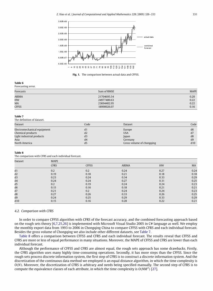
0.2631]. The mean absolute percentage error (MAPE) and the root mean squared error (RMSE), both of which are the mostcommonly used error measures in business, are used to evaluate the forecast models in this paper [24].The results of these analyses are summarized in Table 6. The data plotted in Fig. 1 consists of 165 (more than 13 years) of

monthly time-points and 166 CFFSS time-points, began in January 1996, and the horizontal coordinate refers to time-pointand the vertical the export volume. Vividly, Fig. 1 reveals the combined forecasting approach fit the actual time series well.Furthermore, as shown in Table 6 CFFSS reduces the RMSE and MAPE of the three individual forecasts, thus it improves theforecasting accuracy of each individual forecast.


Fig. 1. The comparison between actual data and CFFSS.

Table 6Forecasting error.

Forecasts Sum of RMSE MAPE

ARIMA 21704695.54 0.20HW 24977400.63 0.22MA 23694402.95 0.22CFFSS 18990026.07 0.16

Table 7The definition of dataset.

Dataset Code Dataset Code

Electromechanical equipment d1 Europe d6Chemical products d2 USA d7Light industrial products d3 Japan d8Asia d4 Germany d9North America d5 Gross volume of chongqing d10

Table 8The comparison with CFRS and each individual forecast.

Dataset MAPECFRS CFFSS ARIMA HW MA

d1 0.2 0.2 0.24 0.27 0.24d2 0.19 0.18 0.21 0.18 0.18d3 0.23 0.24 0.34 0.33 0.29d4 0.24 0.24 0.27 0.31 0.25d5 0.2 0.19 0.24 0.24 0.23d6 0.15 0.16 0.18 0.21 0.21d7 0.21 0.2 0.24 0.24 0.23d8 0.27 0.26 0.33 0.26 0.25d9 0.24 0.25 0.29 0.33 0.29d10 0.15 0.16 0.28 0.22 0.21

4.2. Comparison with CFRS

In order to compare CFFSS algorithm with CFRS of the forecast accuracy, and the combined forecasting approach basedon the rough sets theory [6,7,25,26] is implemented with Microsoft Visual Studio 2005 in C# language as well. We employthe monthly export data from 1993 to 2006 in Chongqing China to compare CFFSS with CFRS and each individual forecast.Besides the gross volume of Chongqing we also include other different datasets, see Table 7.Table 8 offers a comparison between CFFSS and CFRS and each individual forecast. The results reveal that CFFSS and

CFRS are more or less of equal performance in many situations. Moreover, the MAPE of CFFSS and CFRS are lower than eachindividual forecast.Although the performance of CFFSS and CFRS are almost equal, the rough sets approach has some drawbacks. Firstly,

the CFRS algorithm uses many highly time-consuming operations. Secondly, it has more steps than the CFFSS. Since therough sets process discrete information system, the first step of CFRS is to construct a discrete information system. And thediscretization of the continuous data method we employed is an equal distance algorithm, in which the time complexity isO(N). Moreover, the discretization of CFRS is arbitrary and needs being specified manually. The second step of CFRS is tocompute the equivalence classes of each attribute, in which the time complexity is O(NM2) [27].


Table 9The comparison of characteristic between CFFSS and CFRS.

Time-consuming Time complexity Restriction Robustness

CFRS High O(N)+ O(NM2) Restricted to ‘‘thin’’ data (large sample and the number ofcomponent forecasts is small in term of sample)

Low

CFFSS Low O(NM) None High

It is a dilemma for CFRS, for if on one hand it is discretized into too many intervals, there will be more time-points forcomputing the conditional entropy or it will throw an exception of dividing by zero when computing the significance ofeach attribute; on the other hand if discretized into too few intervals then it will be so rough for extracting each individualforecast’s feature that we cannot get a weight vector for combined forecasting with high forecasting accuracy. In otherwords, the process of computing conditional entropy tends to throw a dividing by zero exception when there is a high ratioof the number of component forecasts time-points i.e. more component forecasts but fewer time-points. So it is not veryrobust in a sense. In our experiments, when the number of individual forecasts is 3 and the number of time-points is 166,discretizing into 4 intervals is suitable for a better result. Whereas when the number of component forecasts is very largeand the number of time-point sets is small, a divide by zero exception for the computing of conditional entropy will alwaysbe thrown.Comparing with the CFRS, CFFSS can achieve an almost equal performance to the CFRS. Obviously, the CFFSS has a

much lower time-consumption and is free from such complex operations as discretization, computing equivalence classand conditional entropy. And its time complexity is only O(NM), while the CFRS is O(N) + O(NM2). In practice, there aremany kinds of data, thus such highly time-consuming operations cannot be afforded. More importantly, since CFFSS is freefrom such operations, there is no such restriction of the number of component forecasts and the number of time-points.Table 9 is the comparison of characteristics between CFFSS and CFRS.

5. Conclusion

This paper proposes a combined forecasting approach based on fuzzy soft sets by using an export dataset of ChongqingMunicipality China from 1993 to 2006 and compares CFFSS with the combined forecasting approach based on the roughsets theory (CFRS) which was proposed by [7], and also with the individual forecasts as well. The empirical results showthat CFFSS outperforms the individual forecast in most situations and is almost equal to CFRS but is a low time-consumingoperation and is free from CFRS’s restriction of the number of component forecasts and the length of observation data. Itis a promising combined forecasting approach and is another new application of soft sets, which has enriched the wideapplication of soft sets theory in real life.The core of this approach is to construct the fuzzy membership function and the tabular form of the fuzzy soft sets

model. This paper uses the accuracy of each time-point as the criterion of fuzzy membership and employs the sum of fuzzymembership to design the determination of weight vector of combined forecasts.Although CFFSS can reduce the error of individual forecasts, the export volume in international trade is affected by

many factors such as supply and demand, and to a large extent, governmental intervention (trade barriers and subsidies),GDP, FDI, interest rate, tax reimbursement, price of labor power, etc. It is difficult to forecast the export volume veryaccurately with a single factor, which requires a multidimensional time series to analyze such a problem. Since themultidimensional time series are always fuzzy and nonlinear, the fuzzy soft sets are very suitable to resolve such a problemwith its parameterization, multi-observer notion in the further study and binary operations. In fact, to it can be addedmultidimensional time series by the notion ofmulti-observers and the use of soft binary operations formore complexmodelconstruction to describe such kinds of problem.

Acknowledgements

Our work is sponsored by the national science foundation of Chongqing, China (CSTC 2006BB2246) and the NationalFunds of Social Science (08XJY007). We would thank Miss Ran for her patience in revising our writing. We also thank theanonymous referees for their constructive remarks that helped to improve the clarity and the completeness of this paper.

References

[1] J.M. Bates, C.W. Granger, The combination of forecasts, Operational Research Quarterly 20 (1969) 451–468.[2] J.P. Dickinson, Some comments on the combination of forecasts, Operational Research Quarterly 26 (1975) 205–210.[3] S. Makridakis, A. Andersen, R. Carbone, R. Fildes, M. Hibon, R. Lewandowski, J. Newton, E. Parzen, R. Winkler, The accuracy of extrapolation (timeseries) methods: Results of a forecasting competition, Journal of Forecasting. 1 (1982) 111–153.

[4] M. Deutsch, C.W. Granger, T. Terasvirta, The combination of forecasts using changing weights, International Journal of Forecasting 10 (1994) 47–57.[5] C.K. Chan, B.G. Kingsman, H. Wong, The value of combining forecasts in inventory management—a case study in banking, European Journal ofOperational Research 117 (1999) 199–210.

[6] B. Zhong, Z. Xiao, Determination to weighting coefficient of combination forecast based on rough set theory, Journal of Chongqing University (NaturalScience). 25 (2002) 127–130.


[7] B. Zhong, Z. Xiao, A compound projection method based on coarse aggregate theory, Statistical Research 11 (2002) 37–39.[8] R. Prudêncio, T. Ludermir, A Machine Learning Approach to Define Weights for Linear Combination of Forecasts, 2006, pp. 274–283.[9] F. Zhang, An application of vector GARCHmodel in semiconductor demand planning, European Journal of Operational Research 181 (2007) 288–297.[10] D. Molodtsov, Soft set theory–first results, Computers & Mathematics With Applications 4/5 (1999) 19–31.[11] L.A. Zadeh, Fuzzy sets, Information and Control 8 (1965) 338–353.[12] P.K. Maji, R. Biswas, A.R. Roy, Soft set theory, Computers & Mathematics With Applications. (2003) 555–562.[13] Hacı Aktaş, Naim Çağman, Soft sets soft groups, Information Sciences 177 (2007) 2726–2735.[14] Y.B. Jun, C.H. Park, Applications of soft sets in ideal theory of BCK/BCI-algebras, Information Sciences 178 (2008) 2466–2475.[15] P.K. Maji, A.R. Roy, An application of soft sets in a decision making problem, Computers & Mathematics With Applications (2002) 1077–1083.[16] Z. Xiao, Y. Li, B. Zhong, X. Yang, Research on synthetically evaluating method for business competitive capacity based on soft set, Statistical Research

(2003) 52–54.[17] M.M. Mushrif, S. Sengupta, A.K. Ray, Texture classification using a novel, soft-set theory based classification algorithm, Lecture Notes in Computer

Science 3851 (2006) 246–254.[18] D. Chen, E.C.C. Tsang, D.S. Yeung, X. Wang, The parameterization reduction of soft sets and its applications, Computers & Mathematics with

Applications 49 (2005) 757–763.[19] A.R. Roy, P.K. Maji, A fuzzy soft set theoretic approach to decision making problems, Journal of Computational and Applied Mathematics 203 (2007)

412–418.[20] Z. Kong, L. Gao, L. Wang, Comment on ‘‘A fuzzy soft set theoretic approach to decision making problems’’, Journal of Computational and Applied

Mathematics (2008).[21] Y. Zou, Z. Xiao, Data analysis approaches of soft sets under incomplete information, Knowledge-Based Systems (2008).[22] P.K. Maji, R. Biswas, A.R. Roy, Fuzzy soft sets, Journal of Fuzzy Mathematics 9 (2001) 589–602.[23] G.E.P. Box, G. Jenkins, Time Series Analysis, Forecasting and Control, Holden-Day, San Francisco, 1990.[24] R.J. Hyndman, A.B. Koehler, Another look at measures of forecast accuracy, International Journal of Forecasting 22 (2006) 679–688.[25] Z. Pawlak, Rough sets, International Journal of Computer and Information Sciences 11 (1982) 341–356.[26] Z. Pawlak, A. Skowron, Rudiments of rough sets, Information Sciences 177 (2007) 3–27.[27] G.Y. Wang, H. Yu, D.C. Yang, Decision table reduction based on conditional information entropy, Chinese Journal of Computers 25 (2002) 759–766.

a combined forecasting approach based on fuzzy soft sets

Documents