a combined local and nonlocal closure model for the

A Combined Local and Nonlocal Closure Model for the Atmospheric Boundary Layer.Part I: Model Description and Testing

JONATHAN E. PLEIM

Atmospheric Sciences Modeling Division,* Air Resources Laboratory, National Oceanic and Atmospheric Administration,Research Triangle Park, North Carolina

(Manuscript received 21 February 2006, in final form 11 September 2006)

ABSTRACT

The modeling of the atmospheric boundary layer during convective conditions has long been a majorsource of uncertainty in the numerical modeling of meteorological conditions and air quality. Much of thedifficulty stems from the large range of turbulent scales that are effective in the convective boundary layer(CBL). Both small-scale turbulence that is subgrid in most mesoscale grid models and large-scale turbulenceextending to the depth of the CBL are important for the vertical transport of atmospheric properties andchemical species. Eddy diffusion schemes assume that all of the turbulence is subgrid and therefore cannotrealistically simulate convective conditions. Simple nonlocal closure PBL models, such as the Blackadarconvective model that has been a mainstay PBL option in the fifth-generation Pennsylvania State Univer-sity–National Center for Atmospheric Research Mesoscale Model (MM5) for many years and the originalasymmetric convective model (ACM), also an option in MM5, represent large-scale transport driven byconvective plumes but neglect small-scale, subgrid turbulent mixing. A new version of the ACM (ACM2)has been developed that includes the nonlocal scheme of the original ACM combined with an eddy diffusionscheme. Thus, the ACM2 is able to represent both the supergrid- and subgrid-scale components of turbulenttransport in the convective boundary layer. Testing the ACM2 in one-dimensional form and comparing itwith large-eddy simulations and field data from the 1999 Cooperative Atmosphere–Surface Exchange Studydemonstrates that the new scheme accurately simulates PBL heights, profiles of fluxes and mean quantities,and surface-level values. The ACM2 performs equally well for both meteorological parameters (e.g., po-tential temperature, moisture variables, and winds) and trace chemical concentrations, which is an advan-tage over eddy diffusion models that include a nonlocal term in the form of a gradient adjustment.

1. Introduction

The limitations of local eddy diffusion models forrepresenting convective conditions in the planetaryboundary layer (PBL) are well known. The basic prob-lem is that eddy diffusion assumes that the turbulenteddies are of a smaller scale than the vertical grid spac-ing of the model. Thus, modeled fluxes are proportionalto local gradients. The convective boundary layer(CBL), however, is characterized by buoyant plumesoriginating in the surface layer and rising up into the

capping inversion. Thus, the subgrid assumption ofeddy diffusion is not valid and fluxes are often counterto the local gradients. For example, upward heat fluxtypically penetrates to �80% of the PBL height (h),while potential temperature gradients are very smallthrough most of the PBL and are often counter to theflux in the upper half of the PBL.

Nonlocal closure schemes have been successful atsimulating convective boundary layer fluxes and pro-files. Many PBL schemes simply add a gradient adjust-ment term (�h) to the eddy diffusion equation (Dear-dorff 1966; Troen and Mahrt 1986; Holtslag and Boville1993; Noh et al. 2003),

��

�t�

�

�z�w��

�

�z ��Kh��

�z� �h��, �1�

where Kh is the vertical eddy diffusivity for heat, � is thepotential temperature, and w�� represents the kine-matic heat flux. Note that these schemes were originally

* In partnership with the U.S. Environmental ProtectionAgency.

Corresponding author address: Jonathan Pleim, AtmosphericSciences Modeling Division, Air Resources Laboratory, NOAA,Research Triangle Park, NC 27711.E-mail: [email protected]

SEPTEMBER 2007 P L E I M 1383

DOI: 10.1175/JAM2539.1

JAM2539

developed for heat flux, and application of the coun-tergradient term to other quantities has been problem-atic. Other PBL schemes represent nonlocal fluxes ex-plicitly using a transilient matrix that defines the massflux between any pair of model layers even if they arenot adjacent (e.g., Stull 1984; Blackadar 1978; Pleimand Chang 1992):

��i

�t�

j

Mij�j , �2�

where Mij is the transilient matrix containing the mixingcoefficients between layers i and j.

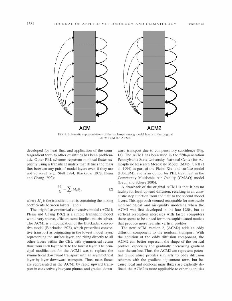
The original asymmetrical convective model (ACM1;Pleim and Chang 1992) is a simple transilient modelwith a very sparse, efficient semi-implicit matrix solver.The ACM1 is a modification of the Blackadar convec-tive model (Blackadar 1978), which prescribes convec-tive transport as originating in the lowest model layer,representing the surface layer, and rising directly to allother layers within the CBL with symmetrical returnflow from each layer back to the lowest layer. The prin-cipal modification for the ACM1 was to replace thesymmetrical downward transport with an asymmetricallayer-by-layer downward transport. Thus, mass fluxesare represented in the ACM1 by rapid upward trans-port in convectively buoyant plumes and gradual down-

ward transport due to compensatory subsidence (Fig.1a). The ACM1 has been used in the fifth-generationPennsylvania State University–National Center for At-mospheric Research Mesoscale Model (MM5; Grell etal. 1994) as part of the Pleim–Xiu land surface model(PX-LSM), and is an option for PBL treatment in theCommunity Multiscale Air Quality (CMAQ) model(Byun and Schere 2006).

A drawback of the original ACM1 is that it has nofacility for local upward diffusion, resulting in an unre-alistic step function from the first to the second modellayers. This approach seemed reasonable for mesoscalemeteorological and air-quality modeling when theACM1 was first developed in the late 1980s, but asvertical resolution increases with faster computersthere seems to be a need for more sophisticated modelsthat produce more realistic vertical profiles.

The new ACM, version 2, (ACM2) adds an eddydiffusion component to the nonlocal transport. Withthe addition of the eddy diffusion component, theACM2 can better represent the shape of the verticalprofiles, especially the gradually decreasing gradientnear the surface. Thus, the ACM2 can represent poten-tial temperature profiles similarly to eddy diffusionschemes with the gradient adjustment term, but be-cause local and nonlocal mass fluxes are explicitly de-fined, the ACM2 is more applicable to other quantities

FIG. 1. Schematic representations of the exchange among model layers in the originalACM1 and the ACM2.

1384 J O U R N A L O F A P P L I E D M E T E O R O L O G Y A N D C L I M A T O L O G Y VOLUME 46

(e.g., humidity, winds, or trace chemical mixing ratios).Thus, the purpose of the ACM2 is to provide a realisticand computationally efficient PBL model for use inboth meteorological and atmospheric-chemistry mod-els. Note that consistent treatment of meteorologicaland chemical species is becoming increasingly impor-tant as more applications involve online coupling ofmeteorological and chemical components.

The development, testing, and evaluation of theACM2 are presented in a series of articles. This workpresents the development, mathematical description,and 1D offline testing of the model. Pleim (2007, here-inafter Part II) describes MM5 simulations using theACM2 and evaluation of results for a 1-month period inthe summer of 2004. A third and forthcoming articlewill present the application and evaluation of CMAQsimulations using ACM2 for the same period and evalu-ation of chemical concentration profiles in comparisonwith aircraft measurements from the InternationalConsortium for Atmospheric Research on Transportand Transformation (ICARTT) study. The ACM2 isalso being included into the Weather Research andForecast (WRF) model.

2. Model formulation

The new model is a combination of local and nonlo-cal closure. In specific terms, the ACM2 is a combina-tion of the original ACM1 (Pleim and Chang 1992) andeddy diffusion. The key technique is to match the twoschemes at a certain height, in this case the top of thelowest model layer, and apportion the mixing rate be-tween the two schemes so that the resultant flux at thatheight is identical to that produced by either schemerunning alone. Note that a reasonably high vertical gridresolution is required, such that the top of the lowestlayer can be considered to be within the surface layer.While sensitivity tests have show some dependence onresolution, particularly in the shape of the lowest partof the profile, the scheme has proven to be robust usingthe lowest layer thicknesses, ranging from 50 m for thelarge-eddy simulation (LES) tests shown in section 3a,down to 4 m for the Global Energy and Water CycleExperiment (GEWEX) Atmospheric Boundary LayerStudy (GABLS) test case shown in section 3c.

First, the nonlocal model development of the ACM1,as shown by Pleim and Chang (1992), is described. Themodel equations are presented here in discrete form ona staggered vertical grid where scalar quantities, such aswater vapor, condensed water species, and trace chemi-cal species, as well as horizontal momentum compo-nents, are located at the layer centers designated by thesubscript i. Vertical fluxes, vertical velocities, and eddydiffusivities are located at the layer interfaces (e.g., i

1⁄2). The nonlocal scheme for any scalar Ci (mass mixingratio) in model layer i is given by

�Ci

�t� MuC1 � MdiCi Mdi1Ci1

�zi1

�zi, �3�

which is identical to Eq. (3) in Pleim and Chang (1992),except that here the vertical dimension is expressed asheight above ground (z) rather than �. Here, Mu is theupward convective mixing rate, Mdi is the downwardmixing rate from layer i to layer i � 1, C1 is the mixingratio in layer 1 (the lowest model layer), and �zi is thethickness of layer i. The downward mixing rate Mdi isderived from Mu according to mass conservation as

Mdi � Mu�h � zi�1�2��zi, �4�

where h is top of PBL. Thus, the flux of C at any modellevel interface (i 1⁄2) is given by

Fi1�2 � Mu�h � zi1�2�C1 � Mdi1�zi1Ci1. �5�

Combining Eq. (5) with Eq. (4) gives

Fi1�2 � Mu�h � zi1�2��C1 � Ci�. �6�

Thus, for the case where C is replaced with virtual po-tential temperature � , Mu can be defined in terms ofkinematic buoyancy flux at the top of the lowest modellayer B1.5 as

Mu � B1.5� ��h � z11�2��1 � ��2��. �7�

Assuming that the top of the lowest model layer is suf-ficiently close to the surface that fluxes are dominatedby small-scale turbulent eddies; the buoyancy flux canbe defined by eddy diffusion as

B1.5 � Kh�z11�2��1 � ��2�

�z11�2, �8�

where the eddy diffusivity Kh is derived from surfacelayer theory as in Eq. (12), shown below. CombiningEqs. (7) and (8) yields convective mixing rate as a func-tion of Kh:

Mu �Kh�z11�2�

�z11�2�h � z11�2�. �9�

Note that the virtual potential temperature gradient isconveniently eliminated from the convective mixingrate definition. Furthermore, because the convectivemixing rate is directly related to eddy diffusivity it issimple to apportion mixing between local and nonlocalcomponents of a combined scheme.

a. Combined local and nonlocal mixing

Combining Eq. (3), which represents the ACM1 non-local scheme, with eddy diffusion gives the ACM2 gov-erning equation in discrete form:


�Ci

�t� M2uC1 � M2diCi M2di1Ci1

�zi1

�zi

1

�zi�Ki1�2�Ci1 � Ci�

�zi1�2

Ki�1�2�Ci � Ci�1�

�zi�1�2�.

�10�

Note that Mu and Md have been replaced with M2uand M2d since the total mixing is now split betweenlocal and nonlocal components by a weighting factorfconv. Thus,

M2u �fconvKh�z11�2�

�z11�2�h � z11�2�� fconvMu and �11a�

K�z� � Kz�z��1 � fconv�.

�11b�

Vertical eddy diffusivity Kz is defined by boundarylayer scaling similarly to Holtslag and Boville (1993) as

Kz�z� � ku*

��zs

L�z�1 � z�h�2, �12�

where k is the von Kármán constant (�0.4), u* is thefriction velocity, and h is the PBL height. For unstableconditions (zs/L � 0), zs � min(z, 0.1h), and for stablecondition zs � z. The nondimensional profile functionsfor unstable conditions, according to Dyer (1974), aregiven by

�h � �1 � 16z

L��1�2

and

�m � �1 � 16z

L��1�4

, �13�

where the Monin–Obukov length scale L is

L �Tou2

*gk�*

, �14�

To represents the average temperature in the surfacelayer, and �* is the surface temperature scale defined asthe surface kinematic heat flux divided by u*. Note thatwhen � in Eq. (12) is replaced by �h, then Kz becomesKh. A schematic of the transport between model layersfor the ACM2 model is shown in Fig. 1b.

It is clear that fconv is the key parameter that controlsthe degree of local versus nonlocal behavior. At eitherextreme ( fconv � 1 or fconv � 0) the scheme reverts toeither the ACM1 nonlocal scheme or local eddy diffu-sion, respectively. For stable or neutral conditions fconv

is set to zero for pure eddy diffusion because the non-

local scheme is only appropriate for convective condi-tions where the size of buoyant eddies typically exceedthe vertical grid spacing. Figure 2 shows vertical pro-files of potential temperature for a series of 1D simu-lations where convective conditions are driven by rap-idly increasing surface temperature (6 K h�1). The pro-files shown are after 6 h of simulation with fixed valuesof the partitioning factor ( fconv) ranging from 0 to 1.The pure eddy diffusion profile ( fconv � 0) shows adownward gradient from the ground up to about 1300m. The eddy diffusion model also results in the highestPBL height. The ACM1 profile ( fconv � 1) has a singlesuperadiabatic layer with a near-neutral profile in thelower PBL gradually becoming more stable with height.The other three profiles are in between where the maineffect of the nonlocal component seems to be to in-crease the stability of the lower 2/3 of the PBL and tolower the PBL height. Whereas, adding the local com-ponent to the ACM1 leads to a more realistic graduallydecreasing superadiabatic profile in the lowest couplehundred meters.

Because the local component depends on the localpotential temperature gradient and the nonlocal com-ponent does not, the value of fconv determines theheight at which the potential temperature gradient goesto zero. As shown in Fig. 2, the higher the value of fconv

the lower the level of zero gradient. Of the variousproportions of local and nonlocal components tested,the test where fconv � 50% seems to give the mostrealistic results. Figure 3 shows that the normalized fluxand potential temperature profiles with fconv � 0.5 arevery similar to the LES profiles for the convectiveboundary layer shown by Stevens (2000). The zero gra-dient level is about 40% of the PBL height in theACM2 simulation as compared with about 46% for theLES results shown by Stevens (2000).

The ACM2 equation [Eq. (10)] is similar to Eq. (1) inthat the vertical fluxes are described by a combinationof a local gradient-driven component and a nonlocalcomponent. There have been many attempts over theyears to provide a theoretical basis for this two-com-ponent form of the heat flux equation (e.g., Deardorff1966, 1972; Holtslag and Moeng 1991). For example,Holtslag and Moeng (1991) showed how Eq. (1) can bederived from the second-order heat flux budget equa-tion, albeit with some simplifying parameterizations.Thus, by following the formulation of models based onEq. (1), an expression for fconv can be derived from theratio of the nonlocal flux term to the total flux as

fconv �Kh�h

Kh�h � Kh

��

�z

, �15�


where �h is the gradient adjustment term for the non-local transport of sensible heat given by Holtslag andBoville (1993) as

�h �aw*�w��o

wm2 h

, �16�

where wm � u*/�m, w* is the convective velocity scale,and the constant a is set to 7.2. Substituting Eq. (16)into Eq. (15) and approximating the surface sensibleheat flux as

�w��o � �ku*�h

zs

��

�z, �17�

where zs � 0.1h, gives

fconv � �1 1

k0.1a

u*w*

�h

�m2 ��1

. �18�

Noting that for the profile functions suggested by Dyer(1974), as shown above in Eq. (13), �h/�2

m � 1, and

u*w*

� k1�3��h

L��1�3

;

then fconv becomes

fconv � �1 k�2�3

0.1a ��h

L��1�3��1

. �19�

Figure 4 shows how fconv, defined according to Eq. (19),behaves as a function of stability. Using this functionfor partitioning the local and nonlocal components ofthe model for all unstable conditions allows for agradual transition from stable and neutral conditions,where local transport only is used, through increasinginstability where the nonlocal component ramps upvery quickly but then levels off at around 0.5. Thisagrees with the test results shown in Figs. 2 and 3 thatsuggest for strongly convective conditions fconv shouldhave a maximum value of about 0.5.

Because the fconv is derived from the model describedby Holtslag and Boville (1993, hereinafter HB93),which is an example of a model represented by Eq. (1),the eddy diffusivity used in ACM2, defined by the com-bination of Eqs. (11b), (12), and (18), is identical to theeddy diffusivity for heat in the HB93 model when thenonlocal term is included in the definition of thePrandtl number (see HB93, their appendix A). Thus,the eddy diffusion terms are the same while the coun-tergradient term in Eq. (1) (Kz�) is replaced by thetransilient terms that involve the nonlocal mass ex-change rates (M2u and M2d). The advantage of theACM2 approach is that the nonlocal mass exchange is

FIG. 2. Potential temperature profiles during convective conditionsfor various nonlocal fractions of turbulent mixing ( fconv).

FIG. 3. Normalized sensible heat flux profile and potential tem-perature profile minus the minimum value using a value offconv � 0.5.


a physical representation of upward transport by de-training convective plumes that applies to any quantity,whereas the models represented by Eq. (1) adjust thelocal potential temperature gradient to account for theeffects of large-scale convection driven by the surfaceheat flux. While such models work well for heat wheresurface heat flux is both the source of the transportedquantity and the driver of the convective turbulence,for other transported quantities the surface heat flux inEq. (16) is replaced by the surface flux of the trans-ported quantity. Thus, nonlocal effects are proportionalto the surface flux, which may be driven by mechanismscompletely unrelated to convective turbulence (e.g.,chemical emissions from mobile or area sources). Fur-thermore, for quantities that have no upward surfacefluxes (e.g., ozone) these models revert to eddy diffu-sion only, but with an eddy diffusivity (assumed to bethe same as for heat) diminished by the nonlocal termin the Prandtl number equation.

b. Diagnostic scheme for determination of PBL height

Many models (e.g., Troen and Mahrt 1986; Holtslagand Boville 1993) diagnose the PBL height h by incre-mental calculation of the bulk Richardson number Ribfrom the surface up to a height at which Rib � Ricrit. Anadvantage of this method is that it can be used for allstability conditions, with the idea that the PBL shouldbe defined as a bulk layer where turbulence predomi-nates. For unstable conditions, however, the PBLshould be considered as composed of a free convectivelayer whose top is the level of neutral buoyancy withrespect to a rising thermal of surface layer air, and as anentrainment zone that is statically stable but turbulent

because of penetrating thermals and wind shear. Thus,the bulk Richardson number method should be appliedover the entrainment layer only. In this way, h is diag-nosed as the height above the level of neutral buoyancywhere Rib computed for the entrainment layer exceedsthe critical value. The advantage of this technique isthat the wind shear in the entrainment zone is consid-ered explicitly rather than the wind speed at height h.Also, the height above ground is not a relevant param-eter in this method, whereas the thickness of the stableentrainment layer is.

For stable conditions the method for diagnosis ofPBL height h is the same as for the previous models:

h � Ricrit

��U�h�2

g��h� � ��z1��, �20�

where � is the virtual potential temperature, z1 is theheight of the lowest model level, and � is the averagevirtual potential temperature between the layer 1 andh. For unstable conditions, first the top of the convec-tively unstable layer (zmix) is found as the height atwhich � (zmix) � �s [where

�s � ��z1� b�w��o

wm

and b � 8.5, as suggested by Holtslag et al. (1990)]. Thebulk Richardson number is then defined for the en-trainment layer above zmix such that

Rib �g��h� � �s��h � zmix�

�� U�h� � U�zmix��2 . �21�

The top of the PBL is diagnosed as the height h whereRib, computed according to Eq. (21), is equal to Ricrit.Note that for some of the LES testing described in thenext section this modified method for diagnosis of PBLheight gave significantly better results, but in MM5 ap-plications the difference was very small.

3. Testing and evaluation

A good PBL model for use in mesoscale meteoro-logical and air-quality modeling should be able to ac-curately simulate the morning growth, maximumheight, and evening collapse of the PBL while predict-ing realistic profiles of temperature, humidity, winds,and other scalar quantities. In a full 3D meteorologicalmodel, simulations are affected by many components ofthe model dynamics and physics, such as radiation,cloud cover, land surface modeling, and large-scale sub-sidence, thus confounding evaluation of the PBLscheme. Therefore, testing of a PBL scheme shouldstart with controlled offline experiments where initial

FIG. 4. Nonlocal fraction of turbulent mixing ( fconv) as afunction of stability.


conditions and surface and dynamic forcings are speci-fied. LESs provide good benchmarks for this type oftesting as shown in the next section, but LESs generallyrepresent quasi-steady conditions and, therefore, donot test the diurnal evolution of PBL simulations. Thenext step in testing is 1D simulations over multiple daysand comparisons with field measurements, as shownbelow in section 3c. Evaluation of the ACM2 in a meso-scale meteorological model will follow in Part II of thispaper and evaluation of the ACM2 in an air-qualitymodel will follow in a subsequent publication.

a. LES testing

A common approach for testing PBL models is bycomparison with LESs (e.g., Hourdin et al. 2002; Noh etal. 2003). While LESs are high-resolution time-depen-dent model simulations, quasi-steady PBL profiles canbe obtained by horizontally averaging across the wholecomputational grid, using periodic boundary condi-tions, and averaging in time over many large-eddy turn-over time periods (� � zi /w*). Ayotte et al. (1996) rana series of LES experiments that were used for com-parison with 16 different 1D PBL schemes. The experi-ments represented cloud-free PBLs driven by shear andbuoyancy. Various stability and wind shear conditionswere generated using constant prescribed forcing bysurface heat flux and geostrophic wind profiles. After aperiod of �5� to spin up turbulent dynamics, passivetracers were added to the simulations and the LES wererun for another �10�, wherein the last 6� were aver-aged to produce the final profiles. The PBL schemeswere initialized from the LES profiles after the 5�spinup, run for �10�, and averaged over the final 6� forcomparison with LES final profiles. See Ayotte et al.(1996) for a detailed description of the LES model andthe simulation experiments.

Three of the 10 cases were chosen to test theACM2—one had a weak capping inversion and a lowvalue of surface sensible heat flux (Q* � 0.05 K m s�1),designated as 05WC, and two had strong capping inver-sions with low (Q* � 0.05 K m s�1) and high (Q* � 0.24K m s�1) values of surface sensible heat flux, labeled05SC and 24SC, respectively. All three cases had aroughness length of 0.16 m, with Ug � 15.0 m s�1 andVg � 0.0 at all levels, and were dry (thus, � � � ). Thevertical grid used for the ACM2 simulation is identicalto the LES vertical grid.

Figure 5 shows potential temperature, u and windcomponents, and tracer profiles for the 05WC experi-ment. The initial profiles were produced after a 3936-sspinup period (�5�) and used to initialize the ACM2simulation. The ACM2 and LES results were comparedfor an averaging period between 3800 and 9120 s afterthe initial state. Note that this was the most difficult ofthe three experiments to replicate because of the weaksurface forcing and the weak capping inversion. How-ever, the ACM2 results compare very closely to theLES results. The slight deviation from the final LESpotential temperature profile is a small cool bias in themixed layer and slightly less penetration into the cap-ping inversion. The -wind-component profiles showvery close agreement, while for the u-wind-componentprofiles the ACM2 results show a bit more gradient inthe middle portion of the PBL. The scalar results alsoshow a tendency to underpredict the upward extent ofthe mixing and the degree of mixing in the lower por-tion of the PBL. Note that these results could be madeto compare more exactly by adjustment of the fconv

parameter and the minimum Kz (now set to 0.1 m2 s�1),but such “tuning” may degrade results of the other ex-periments.

Figure 6 shows the results of the 05SC experiment

FIG. 5. (left) Potential temperature, (middle) wind speed, and (right) tracer profiles by LES and the ACM2 forexperiment 05WC.


that differ from those of 05WC, primarily in thestrength of the capping inversion. The combination ofweak surface forcing and a strong constraint on theextent of mixing makes for smaller differences betweenthe ACM2 and LES results. The potential temperatureand -component wind profiles compare almost exactly,while the u-component and scalar profiles again showthat the ACM2 profiles have slightly greater gradientsin the middle levels of the PBL than the LES results.

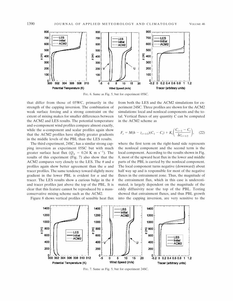
The third experiment, 24SC, has a similar strong cap-ping inversion as experiment 05SC but with muchgreater surface heat flux (Q* � 0.24 K m s�1). Theresults of this experiment (Fig. 7) also show that theACM2 compares very closely to the LES. The � and profiles again show better agreement than the u andtracer profiles. The same tendency toward slightly moregradient in the lower PBL is evident for u and thetracer. The LES results show a curious bulge in the �and tracer profiles just above the top of the PBL. It isclear that this feature cannot be reproduced by a mass-conservative mixing scheme such as the ACM2.

Figure 8 shows vertical profiles of sensible heat flux

from both the LES and the ACM2 simulations for ex-periment 24SC. Three profiles are shown for the ACM2simulations: local and nonlocal components and the to-tal. Vertical fluxes of any quantity C can be computedin the ACM2 scheme as

Fc � M�h � zi1�2��C1 � Ci� Ki�Ci1 � Ci

�zi1�2�, �22�

where the first term on the right-hand side representsthe nonlocal component and the second term is thelocal component. According to the results shown in Fig.8, most of the upward heat flux in the lower and middleparts of the PBL is carried by the nonlocal component.The local component turns negative (downward) abouthalf way up and is responsible for most of the negativefluxes in the entrainment zone. Thus, the magnitude ofthe entrainment flux, which in this case is underesti-mated, is largely dependent on the magnitude of theeddy diffusivity near the top of the PBL. Testingshowed that entrainment fluxes, and thus PBL growthinto the capping inversion, are very sensitive to the

FIG. 6. Same as Fig. 5, but for experiment 05SC.

FIG. 7. Same as Fig. 5, but for experiment 24SC.


minimum value specified for Kz. It was also found thatusing the maximum of the PBL scaling form for Kz [Eq.(12)] and a local formulation that accounts for verticalwind shear was an important improvement for gettinggood agreement at the top of the PBL. The formulationfor the local scaling version of eddy diffusivity is shownin Part II.

b. Comparisons with other PBL models

To get a better understanding of the ACM2’s capa-bilities, it is useful to compare with other PBL models.These LES experiments provide an excellent controlledlaboratory for such comparisons. The 05WC case is se-lected for comparisons between the ACM2, the ACM1,and the HB93 model. This set of models was chosenbecause they are closely related and therefore easilycomparable. The ACM2 has the same nonlocal compo-nent as the ACM1 (although diminished by fconv), whilethe HB93 model has the same eddy diffusion compo-nent as the ACM2, but with a different form of nonlocalparameterization. It is interesting to see what advan-tage the addition of the eddy diffusion component af-fords over the purely nonlocal ACM1 scheme. Also, thecomparison with HB93 shows the relative validity ofthe ACM1 approach to nonlocal effects versus the gra-dient adjustment approach for heat, momentum, andtwo types of tracers. Note that all three schemes are runusing identical modeling infrastructure, including sur-face layer parameterizations and PBL height calcula-tions, in order to directly compare transport algorithms.Therefore, because the eddy diffusion plus the counter-gradient term model is not run exactly as described by

HB93, it is referred to eddy plus nonlocal (EDDYNL)rather than HB93 to make clear that the results shownare not exactly what the HB93 model would produce.

Figure 9 shows the potential temperature, the u and wind components, the same tracer shown in Figs. 5–7that is designated C, and an additional tracer that has anonzero surface boundary condition, designated B. Theinitial profiles have been omitted from each plot, andthe scale on the potential temperature plot (Fig. 9a) hasbeen expanded. Note that the EDDYNL model in-cludes a nonlocal term for potential temperature andthe B tracer only. The nonlocal term for potential tem-perature is given by Eq. (16) and for the B tracer whenthe surface heat flux is replace by the B flux resultingfrom the surface boundary condition (Bsurf � 15 arbi-trary units).

While all three models compare reasonably well tothe LES results for potential temperature, the ACM2results are closest to the LES profile both at the surfaceand near the top of the neutral layer. The EDDYNLmodel profile has a similar shape but is a bit warm atthe surface, cool at the top of the neutral layer, and alittle low for PBL height. Note that if the PBL height iscomputed as described by HB93, the resulting profileshows a much higher PBL that is even higher than theLES result (not shown). The ACM1 shows a small coolbias at the surface and warm bias with more stablegradient near the top of the neutral layer. Comparisonbetween ACM2 and ACM1 shows the importance ofthe eddy diffusion component for realistic gradients inthe surface layer.

The wind profiles (Fig. 9b) show more distinct dif-ference among the models, especially for the u compo-nent. The ACM2 u component profile has a shape mostclosely resembling the LES results, even though it hasmore gradient in the middle portion of the PBL. Whilethe ACM1 u profile is the most nearly constant withheight through most of the mixed layer, like the LES, ithas a considerable low bias throughout most of thePBL. The EDDYNL shows the most diffusive u profileand further evidence of an underpredicted PBL height.Note that Noh et al. (2003) have implemented a non-local term for momentum in a similar model that showsimproved u profile results for similar LES experimentsthat are much like the ACM2 results shown here. Theseresults suggest that both local and nonlocal componentsare important for momentum transport because theshape and magnitude of the ACM2 profile is closer tothe LES profile than either the ACM1, which has nolocal component, or EDDYNL, which has no nonlocalcomponent. However, even the ACM2 profile showsconsiderable discrepancy from the LES result, suggest-ing that intermediate scales of turbulent eddies that are

FIG. 8. Profiles of sensible heat flux. Local, nonlocal, and totalsensible heat flux are compared with LES sensible heat flux.


neglected in this scheme may be important for momen-tum transport in the mid-PBL layers.

The C tracer results (Fig. 9c) show almost identicalprofiles for ACM1 and ACM2, but with a bit moregradient than the LES profile and lower values near thesurface. The EDDYNL profile shows even lesser valuesin the lower layers because of the lower PBL heightthat results in less entrainment of the higher C valuesaloft. The B tracer profiles, shown in Fig. 9d, also showclose similarity between ACM1 and ACM2, but with amore continuous curve in the lowest layers for ACM2.The near-surface overprediction by the EDDYNLmodel is again attributable to the underprediction ofPBL height. As with the C tracer profiles, all threemodels produce B tracer profiles with more gradient inthe mid-PBL layers than the LES. This may again re-flect the inability of these simple models to include thefull range of eddy scales between the subgrid scales thatdrives the eddy diffusion term and the PBL scale of thenonlocal components.

c. GABLS experiment

The second intercomparison project from the GABLSis based on 3 days from the Cooperative Atmosphere–

Surface Exchange Study 1999 (CASES-99) experimentand aims to study the representation of the diurnalcycle over land in both 1D column models and LESs.Simple initial conditions and forcing in the form of sur-face temperature, geostrophic wind velocity, and large-scale subsidence were provided. The ACM2 was one of23 1D models that simulated the experiment. The ex-periment setup and preliminary results of the modelintercomparison and evaluation through comparisonwith observations can be found online (http://www.misu.su.se/�gunilla/gabls/). The results shown here arelimited to comparison of the ACM2 simulations withCASES-99 measurements.

Figure 10 shows the 2-m air temperature simulatedby the ACM2 along with measurements at 1.5 m on themain tower and 2 m from six surrounding towers. Themodel results follow the measurements very closelywith the exception of the lowest temperatures on thesecond night (hours 46–52). Daytime peak tempera-tures are especially well simulated. The 10-m windspeed simulated by the ACM2, however, departs sig-nificantly from the observations, especially during thedaytime (Fig. 11). There is good agreement during theearly morning hours (24–32) with an abrupt jump

FIG. 9. Comparison of ACM2, ACM1, and EDDYNL (Holtslag and Boville 1993) with the05WC LES experiment for (a) potential temperature, (b) wind components, (c) B tracer, and(d) C tracer.


around 0900 LT. The observations show higher windspeeds during the day that are fairly constant (4–6 ms�1), while the ACM2 has a morning dip and afternoonpeak. According to the preliminary analysis of the GA-BLS model intercomparison presented by Svenssonand Holtslag (2006) the ACM2 produced the highestpeak afternoon wind speed of all of the models tested.Clearly, winds are very difficult to model with a 1Dsimulation using a very simple setup and constant geo-strophic forcing. However, one of the things to look forin the MM5 simulations, discussed in Part II, will beevidence of afternoon overpredictions in wind speed.

The surface sensible heat flux simulated by theACM2 is compared with eddy covariance measure-

ments at 1.5 m on the main tower and shown in Fig. 12.Except for some morning underprediction, the mod-eled heat fluxes compare very well to the measure-ments. Figures 13 and 14 show potential temperatureand wind speed from a radiosonde launched at 1900UTC 23 October 1999 (hour 38) from Leon, Kansas,(about 5 km northwest of the main tower) in compari-son with the ACM2 simulations. These soundings showthat the ACM2 has produced a very accurate afternoonPBL height. The lower part of the potential tempera-ture profile, however, seems to show some discrepancyin the gradient near the surface. To examine this fur-ther, Fig. 15 shows temperature measurements at sixheights on the 55-m main tower and demonstrates that

FIG. 11. Same as Fig. 10, but for 10-m wind speed.

FIG. 10. The 2-m temperature for the GABLS experiment simulated by the ACM2 incomparison with measurements at seven towers from the CASES-99 experiment.


the near-surface profile produced by the ACM2 is fairlyaccurate. Note that the ability to produce such curvinggradients near the surface is one of the key improve-ments over the original ACM1.

4. Summary

Both the LES and GABLS experiments demonstratethat the ACM2 is able to simulate realistic PBL heights,temperature profiles, and surface heat fluxes. TheACM2 provides a simple solution to the problem ofmodeling both the small- (subgrid) and large-scale tur-bulent transport within convective boundary layers. Asa consequence, the profiles of both heat flux and po-

tential temperature can be realistically simulated. Forthe turbulent transport of heat in the convective bound-ary layer the ACM2 has similar capabilities to themodified eddy diffusion scheme with the gradient ad-justment term. In fact, the same formulation for thegradient adjustment term is used for deriving the par-titioning of the local and nonlocal mixing componentsin the ACM2. The advantage of the ACM2 is that thelocal and nonlocal mixing rates are defined in terms ofthe bulk physical characteristics of the PBL and areequally applicable to any transported quantity.

The LES experiments show that the importance ofadding the eddy diffusion component to the originalACM1 is most evident for quantities that have large

FIG. 13. Potential temperature profiles from the ACM2 simu-lation and a rawinsonde launched from Leon at 1900 UTC (1400LT) 23 Oct 1999.

FIG. 14. Wind speed profiles from the ACM2 simulation and arawinsonde launched from Leon at 1900 UTC (1400 LT) 23 Oct1999.

FIG. 12. Surface sensible heat flux from the ACM2 simulation and measured at 1.5-mheight on the main tower of the CASES-99 experiment (23–24 Oct 1999).


surface fluxes (either positive or negative), such as heatand momentum. Simulation of realistic profiles of suchquantities in the surface layer clearly requires a down-gradient flux component. The profiles of the B and Ctracers, on the other hand, showed very little differencebetween ACM2 and ACM1.

The ACM2 has been incorporated into the MM5 andcoupled to the Pleim–Xiu land surface model. TheACM2 is also being added as a PBL model option tothe WRF model. The capabilities of the ACM2 for usein mesoscale meteorological modeling are demon-strated in Part II, and the capabilities of the ACM2 foruse in air-quality modeling will be demonstrated in afuture paper.

Acknowledgments. The author thanks Keith Ayottefor providing the results of his large-eddy simulations.The author also acknowledges the chair of GABLSProf. Bert Holtslag and the coordinator of the secondintercomparison experiment Dr. Gunilla Svensson fororganizing the GABLS experiment and providing thesetup and description of the modeling study. The re-search presented here was performed under theMemorandum of Understanding between the U.S. En-vironmental Protection Agency (EPA) and the U.S.Department of Commerce’s National Oceanic and At-mospheric Administration (NOAA) and under Agree-ment DW13921548. This work constitutes a contribu-tion to the NOAA Air Quality Program. Although ithas been reviewed by EPA and NOAA and approvedfor publication, it does not necessarily reflect their poli-cies or views.

REFERENCES

Ayotte, K. W., and Coauthors, 1996: An evaluation of neutral andconvective planetary boundary-layer parameterizations rela-tive to large eddy simulations. Bound.-Layer Meteor., 79,131–175.

Blackadar, A. K., 1978: Modeling pollutant transfer during day-time convection. Preprints, Fourth Symp. on AtmosphericTurbulence, Diffusion, and Air Quality, Reno, NV, Amer.Meteor. Soc., 443–447.

Byun, D., and K. L. Schere, 2006: Review of the governing equa-tions, computational algorithms, and other components ofthe models-3 Community Multiscale Air Quality (CMAQ)modeling system. Appl. Mech. Rev., 59, 51–77.

Deardorff, J. W., 1966: The counter-gradient heat flux in thelower atmosphere and in the laboratory. J. Atmos. Sci., 23,503–506.

——, 1972: Theoretical expression for the counter-gradient verti-cal heat flux. J. Geophys. Res., 77, 5900–5904.

Dyer, A. J., 1974: A review of flux-profile relationships. Bound.-Layer Meteor., 7, 363–372.

Grell, G. A., J. Dudhia, and D. Stauffer, 1994: A description of thefifth-generation Penn State/NCAR Mesoscale Model(MM5). NCAR Tech. Note TN-398STR, 138 pp.

Holtslag, A. A. M., and C.-H. Moeng, 1991: Eddy diffusivity andcountergradient transport in the convective atmosphericboundary layer. J. Atmos. Sci., 48, 1690–1698.

——, and B. A. Boville, 1993: Local versus nonlocal boundary-layer diffusion in a global climate model. J. Climate, 6, 1825–1842.

——, E. I. F. De Bruijn, and H.-L. Pan, 1990: A high resolution airmass transformation model for short-range weather forecast-ing. Mon. Wea. Rev., 118, 1561–1575.

Hourdin, F., F. Couvreux, and L. Menut, 2002: Parameterizationof the dry convective boundary layer based on a mass fluxrepresentation of thermals. J. Atmos. Sci., 59, 1105–1123.

Noh, Y., W. G. Cheon, S. Y. Hong, and S. Raasch, 2003: Improve-ment of the K-profile model for the planetary boundary layerbased on large eddy simulation data. Bound.-Layer Meteor.,107, 401–427.

Pleim, J. E., 2007: A combined local and nonlocal closure modelfor the atmospheric boundary layer. Part II: Application andevaluation in a mesoscale meteorological model. J. Appl. Me-teor. Climatol., 46, 1396–1409.

——, and J. S. Chang, 1992: A non-local closure model for verticalmixing in the convective boundary layer. Atmos. Environ.,26A, 965–981.

Stevens, B., 2000: Quasi-steady analysis of a PBL model with aneddy-diffusivity profile and nonlocal fluxes. Mon. Wea. Rev.,128, 824–836.

Stull, R. B., 1984: Transilient turbulence theory. Part I: The con-cept of eddy-mixing across finite distances. J. Atmos. Sci., 41,3351–3367.

Svensson, G., and A. A. M. Holtslag, 2006: Single column mod-eling of the diurnal cycle based on CASES99 data—GABLSsecond intercomparison project. Preprints, 17th Symp. onBoundary Layers and Turbulence, San Diego, CA, Amer.Meteor. Soc., CD-ROM, 8.1.

Troen, I., and L. Mahrt, 1986: A simple model of the atmosphericboundary layer: Sensitivity to surface evaporation. Bound.-Layer Meteor., 37, 129–148.

FIG. 15. Temperature profiles from the ACM2 simulation andthe 55-m main CASES-99 tower at 1900 UTC (1400 LT) 23 Oct1999.


a combined local and nonlocal closure model for the

Documents