1

A comparative analysis of ability of mimicking portfolios

in representing the background factors

Hossein Asgharian*

Department of Economics, Lund University

Box 7082 S-22007 Lund, Sweden

Phone: +4646 222 8667

Fax: +4646 222 4118

Hossein.Asgharian@nek.lu.se.

www.nek.lu.se/nekhas

Abstract

Our aim is to give a comparative analysis of ability of different factor mimicking portfolios in

representing the background factors. Our analysis contains a cross-sectional regression

approach, a time-series regression approach and a portfolio approach for constructing factor

mimicking portfolios. The focus of the analysis is the power of mimicking portfolios in the

asset pricing models. We conclude that the time series regression approach, with the book-to-

market sorted portfolios as the base assets, is the most proper alternative to construct

mimicking portfolios for factors for which a time-series of factor realisation is available. To

construct mimicking portfolios based on the firm characteristics we suggest a loading

weighted portfolio approach.

JEL G12.Keywords: mimicking portfolio; asset pricing; multifactor model; cross-sectional regressionapproach; time series regression approach

* We are very grateful to The Bank of Sweden Tercentenary Foundation for funding this research.

2

1 Introduction

A factor mimicking portfolio is a portfolio of assets constructed to stand for a

background factor. This design is usually preferred to directly using the factor when

its realisations are not returns. By this approach we use only the information captured

in the economic factors, which is relevant for asset returns and reduce the noise in our

asset pricing model (see for example Vassalou, 2000 and Chan et al, 1998 and 1999

for building mimicking portfolios based on the macroeconomic variables). In

addition, a mimicking portfolio may represent an unobservable factor when the stock

sensitivities to the factor are believed to be disclosed by some firm characteristics. A

well-known example of this case is in the Fama and French (1993), where the

characteristics such as firm size or book-to-market ratio are supposed to reveal the

loadings of the firms to some latent distress factors.

Despite the fact that mimicking portfolios are widely applied both in asset pricing

analyses and portfolio valuations, there is no research on the power of the different

methods of constructing these portfolios. The purpose of this paper is to shed light on

the characteristics of the different factor mimicking portfolios and to give a

comparative analysis of these portfolios.

There are several approaches to construct factor mimicking portfolios. A formal

approach is to use cross-sectional regression of returns on factor loadings or firm

characteristics to estimate the return of the mimicking portfolios, henceforth denoted

by the cross-sectional regression approach (CSR), (see Fama, 1976). Another method

that is to some extent equivalent to the regression approach is to construct a portfolio

by going long on stocks with high loadings on a factor while short-selling stocks with

low loadings, henceforth denoted by the portfolio approach (see for example Fama

and French, 1993 and Chan et al, 1998 and 1999). An alternative method, initiated by

Breeden et al (1989), is to define a mimicking portfolio as a projection of a factor into

the asset return space using a time series regression, henceforth denoted by the time-

series regression approach (TSR), (see for example Vassalou, 2000). This approach is

only relevant when a factor realisation is available. Therefore, this method can be

3

used to form portfolios mimicking macroeconomic variables, while it is not applicable

to construct mimicking portfolios based on firm characteristics.

The first part of the paper compares the CSR approach and the portfolio approach. In

the portfolio approach the common practice is to form either equally weighted

portfolios (see Chan et al., 1998) or value weighted portfolios (see Fama and French,

1993). These weighting methods in contrast to the CSR approach do not consider the

relative differences among loadings in portfolio formation. To deal with this problem

we suggest a weighting method based on the relative distances of the loadings.

Moreover, to be able to interpret the estimated coefficients of the monthly CSR as the

returns of the mimicking portfolios we need to normalise the explanatory variables of

the regressions. We employ two alternative approaches for normalisation. To

construct mimicking portfolios, in addition to the estimated asset loadings on the

world market index and several macro variables, we use some firm specific variables.

We use the standard deviations of the mimicking portfolios, the estimated factor risk

premia and the correlations between the portfolios to compare the portfolios

mimicking each factor across different methods.

The second part of the paper studies mimicking portfolios formed based on the TSR

approach. This method is applicable only for factors with available time series

representation. We use therefore the world market index and several macro variables

as the background factors. We analyse the sensitivity of the constructed portfolios to

the choice of the based assets the assets that are used to construct the mimicking

portfolios. Our metrics of comparison is again the standard deviations and the mean

excess returns of the mimicking portfolios and the correlations between the portfolios.

Finally we analyses the ability of the different approaches in representing the

background factors from an asset pricing perspective. We first estimate a multifactor

model for ten industrial portfolios, when the factors are represented by their original

factor realisation. The risk free components of the factors, and consequently the factor

risk premia, are not observed when the factors are not portfolio returns. To solve this

problem we estimate the model by using a maximum likelihood approach, where the

risk free part of each factor is estimated endogenously as an unknown parameter. The

ability of the factor model in explaining the industry mean excess returns is assessed

by a likelihood ratio test. In the next step, we estimate the multifactor model while the

original factor realisations are replaced by the factor mimicking portfolios. The results

4

of the asset pricing tests and parameter estimations are then compared across different

factor representations. The purpose of this analysis is not to attain a sufficient factor

model but to investigate the accuracy of the factor mimicking portfolios.

It is worth noting that it is not common practice to construct mimicking portfolio for

the market factor, because the factor realisations are already portfolio returns.

However, the market factor is expected to be the most import factor and therefore can

be extremely valuable for comparison of the power of the different methods of

constructing mimicking portfolios.

The result of the comparison of the univariate CSR approach with the portfolio

approach shows a high correlation between the CSR and our suggested loading

weighted portfolio approach. This depends on the fact that both approaches consider

the relative distances among the loadings. The analysis of standard deviations shows

that the weighting method that gives higher weights to the larger loadings results in

higher standard deviations of mimicking portfolios. The value weighted approach has

a very low similarity with other methods, which is due to the ad-hoc nature of this

weighting method. Comparing TSR approach based on different base assets shows

that the correlations between mimicking portfolios and the original series are

relatively high for the world market portfolio. However, for most of the

macroeconomic factors the correlations are very low. Regarding both the correlation

analysis and the statistics of the mimicking portfolios we may conclude that the TSR

approach is to some extent sensitive to the choice of the base assets.

In the asset pricing analysis, the model with the original factors is not rejected, while

the CSR and the portfolio approaches are both found to be extremely weak in

explaining the industry mean excess returns. The TSR model with size-sorted

portfolios as the base assets have some significant intercepts and is therefore rejected

even by the likelihood ratio test while the TSR model with book-to-market sorted

base assets is very strong both in the separate t-tests and the joint likelihood ratio test.

Analysing the parameters of the factor models shows that the effects of the different

factors on mean industry excess returns seem to be to some extent different across the

models. The model with the original factors and the TSR-BM model with book-to-

market sorted base assets are relatively similar, particularly with respect to the effect

of the market factor.

5

The outline of the paper is as follows: section 2 discusses the methods for the

construction of the factor mimicking portfolios; test of asset pricing models is

described in section 3; section 4 presents the data; the empirical results and the related

analyses are given in the section 5 and section 6 concludes the paper.

2 Mimicking portfolios

The purpose is to construct a portfolio with a mean return equal to the risk premium

of a background factor and with a beta equal to one against the factor (see Cochrane,

2001). There are two approaches which are in essence different: the first method is to

use cross-sectional regressions (CSR) of the excess returns on the observed/estimated

factor loading, while the other approach uses instead a time-series regression (TSR) of

an observable background factor on the excess returns. There is also a portfolio

approach that is basically related to the CSR method.

2.1 Cross-sectional regression approach, CSR

This method is applicable both when the background factor has a time series

realisation, usually not as a portfolio return, and when the factor is not observable self

but firms’ loading on the factor is mirrored in some firm specific variable. To use the

CSR approach we require the firms’ factor loadings. The loadings are available in the

latter case in the form of the firm specific variables, while in the former case we can

use a time series regression of asset returns on the observed factor realisation to

estimate the factor loading for each firm.

To construct the mimicking portfolios we run the following cross-sectional regression

model for each period, t, t=1,....,T:

,1

0 itikt

K

kkttit uxR ++= ∑

=

γγ (1)

where Rit is the return in excess of the risk free rate for asset i at time t, xikt is the value

of the kth explanatory variable for asset i at t, and uit is an idiosyncratic error. The

values of the k:th explanatory variable in this regression are the loadings of the N

assets on the factor k. The least square estimate of the γkt is the return of the

mimicking portfolio for factor k. It can be written as (see Fama, 1976):

6

KkforRw it

N

iiktkt ,....,0

1== ∑

=

γ (2)

where wikt is element (k+1,i) of the (( K+1) × N) matrix Wt. This matrix is defined as:

( ) ,tttt XXXW 1 ′′= − (3)

where Xt is a (N×(K+1)) matrix of all explanatory variables including a vector of ones

for intercept. We have the following characteristics for the weights wikt:

==

=∑= Kkfor

kforw

N

iikt ,...10

01

1(4)

Therefore, for all k > 0, γkt can be interpreted as the return at time t on a zero

investment portfolio with weight vector wkt on N base assets. We also have

≠=

=∑= kjfor

kjforxw ijt

N

iikt 0

1

1(5)

which implies that the loading of the portfolio with weights wikt should be equal to

one against the factor k and zero against the other factors. In addition, E[γkt] gives the

risk premium of the factor k.

This approach despite all its desired properties has some major drawbacks. The first

problem is due to the fact that the loadings are not usually observable and should be

estimated. This induces the errors in variables problem and may result in bias in

estimated γkt. The second problem is when we use accounting data to represent the

relative asset loadings on the factors. The reason is that the magnitude of γkt depends

on the size of the corresponding xikt. Thus, γkt may be incomparable across the k

factors. One possibility is to normalize explanatory variables in such a way that the

xikt-values fall within the same range for all k. Chan et al. (1998) rank all the loadings

and then normalised them between 0 and 2, but then the relative distances between the

loadings will change. Henceforth, we denote this approach by rank. Our suggestion is

to define *iktx as:

( )( ) ( ) ,

minmaxmax12*

−

−−×=

iktiikti

iktiktiikt xx

xxx (6)

7

This approach, henceforth denoted by distance, leaves the relative distances among

the loadings unchanged. The multiplication by 2 is to have approximately the same

range for *iktx as the market beta.

The observed variables, particularly those from accounting data, are related to each

other. The regression approach, in a multivariate framework, makes it possible to

filter out the shared components. However, our aim is to compare the mimicking

portfolios across different approaches and since the multivariate setting is not possible

for some of the other approaches employed in this paper we apply only the univariate

framework in this study.

2.2 Portfolio approach

An alternative approach that is essentially based on the same idea as the CSR method

is the portfolio approach. This method, however, may be less subject to the errors in

variables and normalising problems discussed in the previous section. Stocks are

sorted according to their factor loadings. Then the stocks with low and high loadings

are grouped in two different portfolios. Finally a factor mimicking portfolio is

constructed by taking a long position in the portfolio with high loadings and a short

position in the portfolio with low loadings on the chosen factor (HmL). The HmL

portfolio, like the portfolios of the regression approach, is a zero investment strategy

that is particularly sensitive to the factor k.

There are several alternative methods to weight the stocks in the high-loading and

low-loading portfolios. The most common alternatives are to form equally weighted

portfolios (e.g. Chan et al., 1998) or to form value weighted portfolios (e.g. Fama and

French, 1993). These weighting methods are somewhat ad hoc and they do not satisfy

the relationship between weights and loadings of the regression approach. In a

univariate case, with k=1, the weight of asset i on the factor k is given by:

( ) ( )∑ ∑∑ ∑∑

= == =

=

−+

−

−=

N

i

N

i iktikt

iktN

i

N

i iktikt

N

i iktikt

xxN

Nx

xxN

xw

1

2

12

1

2

12

1 (7)

8

This gives a perfect correlation between wikt and xikt.1 To maintain this link, our

suggestion is to weight the stocks by their relative distance of the loadings. The

weight of the asset i in the portfolio with low loading on factor k is computed as:

( )( ) ( ) ,

minmaxmin1

iktiikti

iktiiktLikt xx

xxw−

−−= (8)

and for the portfolio with high loading the weight is:

( )( ) ( ) ,

minmaxmax1

iktiikti

iktiktiHikt xx

xxw−

−−= (9)

We then normalize the weights in order to sum to one. This method results in perfect

correlation between xikt and wikt within each portfolio, which makes the method

consistent with the theoretical requirements outlined above.

We use all the three alternative methods to construct low and high portfolios:

weighting all stocks equally (EW), weighting all stocks by their relative market value

(EW) and weighting all stocks by their relative loadings (LW). Note that for the

portfolio with low loadings the stocks are ranked in reverse order.

2.3 The volatility of mimicking portfolios

One metric to assess the importance of the factors in explaining return covariation is

the volatility of the factor mimicking portfolio constructed as zero investment strategy

either by the CSR approach or the portfolio approach. Consider a mimicking portfolio

(mp) constructed by going long on the high loading portfolio (H) and going short on

the low loading portfolio (L):

,lLl

lhHh

hmp RwRwR ∑∑∈∈

−= (10)

1 The relationship between weights and the values of the explanatory variable can be written as:

( ) ( ) ,and

,

1

2

12

1

2

12

1

∑ ∑∑ ∑∑

= == =

=

−=

−

−=

+=

N

i

N

i iktiktN

i

N

i iktikt

N

i ikt

iktikt

xxN

NbxxN

xa

bxaw

which yields:

corr(wikt,xikt) = 1

9

( ) ,2var ∑∑∑∑∑∑∈ ∈∈ ∈∈ ∈

−+=Hi Lj

ijjiLi Lj

ijjiHi Hj

ijjimp wwwwwwR σσσ

( ) ,222var 22 ∑∑∑ ∑∑ ∑∑∈ ∈∈ ∈≠∈ ∈≠+∈

−++=Hi Lj

ijjiLi Lij

ijjiHi Hij

ijjiLHi

iimp wwwwwwwR σσσσ

The first term is the sum of the all variances. The second and third terms are sum of

the covariances within each group H and L. The last term is the sum of all the cross-

covariances. The stronger is the factor for explaining the return covariation the higher

will be within group covariances and the smaller will be the cross-covariances, which

results in a larger var(Rmp).

The volatility of the mimicking portfolio can also be used to compare different

weighting methods because if a factor is important we expect a large return volatility

for a portfolio that goes long on assets with high factor loadings and goes short on

assets with low factor loadings. To see this consider the following one-factor model:

.,....,1 NifR itktikiit =++= εβα (11)

[ ] [ ] S=′= ttt EE εεε ,0

The variance of a portfolio of the assets can then be written as:

( ) ( )

ijj

N

i

N

jijij

N

i

N

jik

ijkjij

N

i

N

jiijj

N

i

N

jip

swwww

swwwwR

∑∑∑∑

∑∑∑∑

+=

+==

ββσ

σββσ

2

2var(12)

The first term is the part of the portfolio variance that is explained by the factor model

while the second term is the unexplained part. Assuming a large number of assets and

that the factor model is adequate to explain the covariations in returns the second term

goes toward zero. In this case, a portfolio that gives relatively larger weights to the

large betas will have a larger variance relative to a portfolio that gives the same

weights to all the assets. Note that the explained part is also driven by the factor

variance, 2kσ .

2.4 Time series regression approach, TSR

One drawback of the approaches above to build the mimicking portfolios for the

factors with available time series observations is that we need to estimate loadings

10

and then construct the mimicking portfolio. This may cause bias due to the errors in

variables problem. The one step time series approach that follows the maximum

correlation portfolio suggested by Breeden et al. (1989) avoid this problem. This

approach is not, however, applicable to build mimicking portfolio when the factor is

not observable and only firms’ loading on the factor are provided by some firm

specific variables.

We estimate the following time series regression of factor k on N asset returns:

.1

0 itit

N

ikikkt Rf ξλλ ++= ∑

=

(13)

where fkt is the factor realisation, Rit is the excess return on the base asset i at time t.

We use the estimated λki as the weights on asset i and form the mimicking portfolio

for factor k as:

.ˆ1

, it

N

ikitk RR ∑

=

= λ (14)

where Rkt is the excess return of the TSR mimicking portfolio, the maximum

correlation portfolio, for factor k at time t. Note that λki are normalised to sum to one.

In equation (13), we can add some control variables, such as other macroeconomic

factors to filter out the overlapping effects. According to Breeden et al. (1989), the

asset betas measured relative to the maximum correlation portfolio are proportional to

the betas measured using the true factor. Despite the differences in estimated betas the

product of the asset beta with the factor risk premium are supposed to be the same for

the original factor model and when using the mimicking portfolio (see Cochrane

2001).

3 Test of asset pricing models

In the absence of arbitrage in large economies the following linear relationship holds

approximately between the expected return on a security and the risk premium

associated with the factors:

µ= lγ0+Bγ, (15)

11

where µ is the (N×1) vector of the expected returns on N assets, l is an (N×1) vector of

ones, γ0 is the riskfree rate of return, and γ is a (K×1) vector of risk premia associated

with K factors. The (N×K) matrix B contains the factor sensitivities of the test assets.

In this paper we have two different econometric approaches, which depends on the

employed factor representation. The first case is when we use the original time series

of the factor realization in the regression model. In the second case the mimicking

portfolios represent the macroeconomic factors.

When we use the original factors in the multifactor model some of the factors are not

asset portfolios and their factor risk premium cannot directly be specified. In this case,

we assume that the risk free part of the factor k, θk, is constant over time and can be

estimated as a parameter of the following factor model:

( ) ,1

it

K

kkktikmtimiit XRR εθββα +−++= ∑

=

(16)

,11

it

K

kktikmtim

K

kkikiit XRR εββθβα +++−= ∑∑

==

TtNi ,.....,1 and ,,.....,1 ==

where Rit is the excess return on asset i at time t, Rmt is the excess return on the market

portfolio, Xkt is realization of the macroeconomic factor k and αi is the unexplained

expected return of asset i.

In the second case the mimicking portfolios represent the macroeconomic factors. The

multifactor model in equation (15) implies the following linear regression model:

,1

1it

K

kktikiit RR εβα ∑

+

=

++= (17)

TtNi ,.....,1 and ,,.....,1 ==

12

where Rkt is the return on factor portfolio k. The explanatory variables include

mimicking portfolios for the market portfolio plus K macroeconomic factors.

Our null hypothesis in both cases is that αi is equal to zero for all i, that is to say the

factors can explain expected excess returns for all the assets. To test the model jointly

for N assets we use the likelihood ratio test:

,~)ln(ln2 2*NLLLR χ−−= (18)

where lnL* and lnL refer to the restricted and unrestricted loglikelihood function

respectively. The likelihood function in the matrix notation is:

( ) ( ) ( ) t

T

tt

TNTL εΣεΣ 1

121det

22ln

2.ln −

=∑ ′−−−= π (18)

where

[ ]′= NTttt εεε 21ε .

are residuals from the restricted/unrestricted model for each of the models in

equations (16) and (17) and Σ is the residual covariance matrix.

4 Data and choice of the factors

The data covers the period 1977 to 1997 and consists of monthly Swedish stock

returns that are corrected for dividends and capital changes like splits etc. The data is

collected from the database ''Trust''. The sample includes all shares excluding banks

and financial firms on the so-called ''A1-listan''. The monthly data on market value of

equity is collected from ''Veckans Affärer”. Data for macroeconomic variables are

from database Ecowin.

We use the following factors:

• Market factors: excess returns on the Morgan Stanley world index computed in

SEK.

13

• Macroeconomic factors: Growth of the industrial production (DIP) is defined as

the percentage change in the monthly industrial production. Slope of the yield

curve (Slope) is the difference between the yield on ten-year government bonds

and the yield on three-month treasury bills. Percentage change in the exchange

rate SEK/USD (DEX).

• Fundamental factors: Book-to-market ratio (BM) is defined by dividing the book

value of the equity from the annual statement to the market value of the firm at the

end of December in each year. Size is estimated for each month as the market

value of equity from the previous month.

For the market and the macroeconomic factors we estimate the loading for each firm

on each of the factors by regressing the excess stock returns on the factor using the

most recent 36 months historical observations before the portfolio formation month.

The estimates are updated each month.

5 Analysis

5.1 CSR approach versus portfolio approach

In this section we compare the univariate CSR approach with the portfolio approach.

Table 1 shows the correlations between different mimicking portfolios. The CSR-

distance and CSR-rank are highly correlated with each other and with the loading

weighted portfolio approach, HmL-LW. The highest correlation as expected is

between the CSR-distance and HmL-LW. This depends on the fact that both

approaches capture the relative distances among the loadings. The value weighted

approach has very low correlations with other methods except for the variable size.

This low correlation reveals the ad-hoc nature of this weighting method.

Table 2 reports the mean returns of the mimicking portfolios. Only BM has a mean

return that is significantly different from zero for all the different methods except

HmL-VW. According to the theoretical discussion in the section 2.1, we may then

conclude that BM is the only priced factor with a positive significant risk premium.

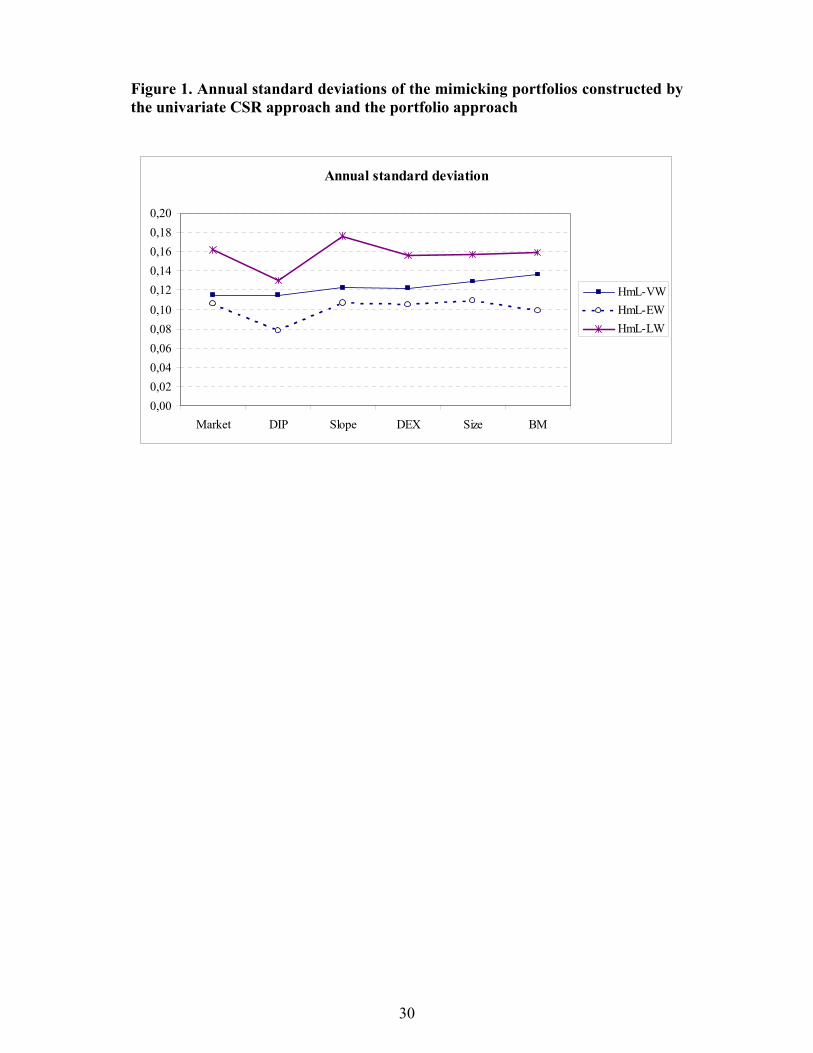
Figure 1 compares the standard deviations of the mimicking portfolios of the portfolio

approach. We have not included the standard deviations of the CSR mimicking

portfolios. The reason is that the level of the standard deviations of these portfolios is

14

related to the way we normalise the loadings in the CSR and may therefore be

misleading. The figure shows that the HmL-LW method that gives higher weights to

the larger loadings as expected results in higher standard deviations (see section 2.3).

The correlation between standard deviations of the HmL-LW and HmL-EW is about

0.87 while the correlations between the HmL-VW and these two methods are around

0.30. This shows that the VW method is not appropriate to judge the relative

importance of the background factors, while the two other methods may give more or

less the same inferences.

5.2 TSR approach based on different base assets

In this section we analyse the sensitivities of the TSR mimicking portfolios to the

choice of the base assets. We use three alternative base assets, i.e., ten size sorted

portfolios, ten book-to-market sorted portfolios, and finally ten randomly sorted

portfolios. Table 3 shows the correlation matrix of these mimicking portfolios and the

original series for each factor. The correlations between mimicking portfolios are

relatively high for the world market portfolio. For the factor DEX the correlations are

also around 0.60. For these two factors the correlations between mimicking portfolios

based on the BM and Size sorted portfolios are higher than the correlations based on

the randomly sorted portfolios. For DIP and Slope the correlations are very low. The

correlations between the mimicking portfolios and the original series are around 0.60

for the market portfolio and much lower for the other factors.

Table 4 shows the statistics of the TSR mimicking portfolios. All the portfolios

mimicking the market have highly significant mean excess returns. The mean excess

returns of the portfolios mimicking DEX are also all significant. The results for DIP

and Slope are in line with the low correlations between the mimicking portfolios and

show a relatively large variation in mean excess return and standard deviation across

different mimicking portfolios.

All in all we find that the TSR approach is to some extent sensitive to the choice of

the base portfolios. Although our base portfolios are formed by using the same

background assets, the sorting characteristics may be important for construction of the

mimicking portfolios.

15

5.3 Mimicking portfolios and asset pricing

In this section we analyse the ability of the mimicking portfolios in representing their

background factors from an asset pricing viewpoint. As the test assets we use ten

industrial portfolios. The purpose is not to find a sufficient factor model to explain the

expected excess returns of the industrial portfolios but to compare the different

choices of the factor mimicking portfolios. Since the results for the portfolio approach

and the CSR approach are very similar we choose to not report the results for both

methods. We use the HmL-LW as the preferred representative of these two groups.

The reason to prefer portfolio approach to the regression approach is that the

properties of the CSR mimicking portfolios may be affected to some extent by our

normalising method. In addition, the CSR approach is probably more exposed to

errors in variable problems comparing to the portfolio approach. The reason to prefer

LW to other weighting methods of the portfolio approach is that this method is

consistent with the theoretical requirements of the mimicking portfolios (as discussed

in the section 2.2).

We first look at the results of the likelihood ratio test in Table 5. Using the model with

the original factors results in a p-value equal to 0.95, which means that the factor

model can explain the expected excess returns of the ten industrial portfolios. This

result does not however hold when switching to the model with the HmL-LW

mimicking portfolios. The p-value is now under the 5%, which rejects the ability of

the model in explaining the industry mean excess returns. The result for TSR depends

on the choice of the base assets. The model with TSR-size mimicking portfolios is

rejected while that with the TSR-BM mimicking portfolios is not. To analyse the

models more in details we start by presenting the estimated parameters given by each

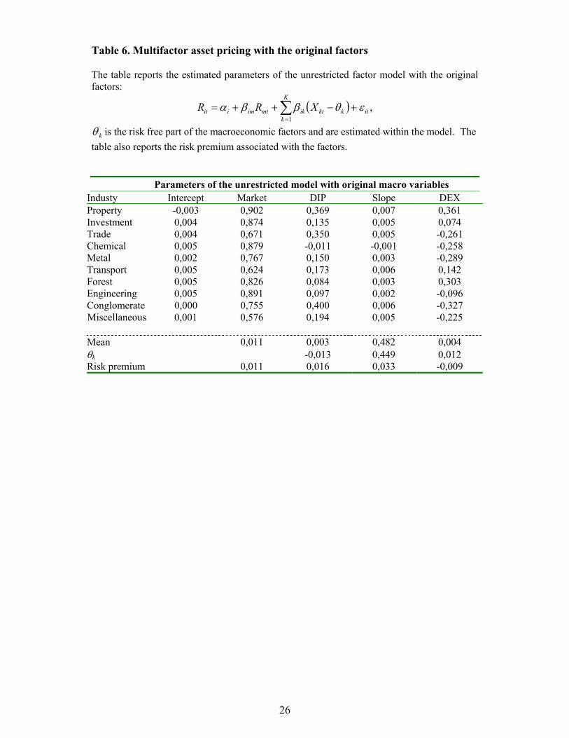
model. Table 6 shows the results for the model with the original factors. The market

beta is less than but close to one for all the industries, revealing that the Swedish

industries have generally lower risk than the world market. The industries exposures

to the factors DIP and Slope are positive except for the Chemical, while the exposures

to the DEX varies in sign by industries. All the factors except DEX have a positive

risk premium.

The results for the models with TSR and HmL-LW mimicking portfolios are reported

in Tables 8 and 9 and 10 respectively. The market betas from the model with the

original factors are in general larger and those from the TSR-BM and smaller than the

16

market betas from the TSR-size. The market betas from the HmL-VW factor model

are all below the betas for three other models (see also Figure 2).

Exposure of the industrial portfolios against the factor DIP varies across the models

(see also Figure 2). The results for the TSR-size, in accordance with the model with

the original factors, show a positive exposure for all the industries except chemical.

However since the estimated risk premium for DIP is negative by this model the

effect of this factor on expected returns will be opposite to that from the model with

the original factors. The model with the TSR-BM mimicking portfolios results in

negative exposures for DIP except for chemical. Due to the negative risk premium,

the effect of DIP on expected returns in this model has the same sign as that in the

model with the original factors. The model with the HmL-LW portfolios gives some

negative and some positive loadings on the factor DIP. Note that the magnitude of the

factor loadings of the model with the original factors is not comparable with that from

other models, except for the market factor, because the factor realisations are not asset

returns. These loadings are therefore not included in Figure 2.

For the factor Slope the exposures are of the same sign for TSR-BM and the original

factors while the Chemical has opposite sign in TSR-size. The risk premium of this

factor is negative in both TSR models. The HmL-LW based model has also positive

loadings for all the industries except Chemical and Miscellaneous, with a positive

factor risk premium.

For the DEX the exposures are approximately of the same sign in the models with the

original factors and TSR-size, while the exposures are mostly positive in the models

with the TSR-BM and HmL-LW.

All in all the effects of the different factors on mean industry excess returns seem to

be to some extent different across the models. Figure 3 illustrates the total impact of

the each factor on industry excess return. For each factor and each industry this is

computed by multiplying the factor risk premium with the industry factor loading.

The total impact of the market factor given by the model with the original factors is

very close to that from the model with TSR-BM. The effects given by TSR-size is

larger for almost all of the industries, while according to the model based on the

HmL-LW mimicking portfolios the market factor does not have any important effect

17

on the mean excess returns. According to the TSR-size based model, the other factors

show mostly negative effects on the mean excess returns.

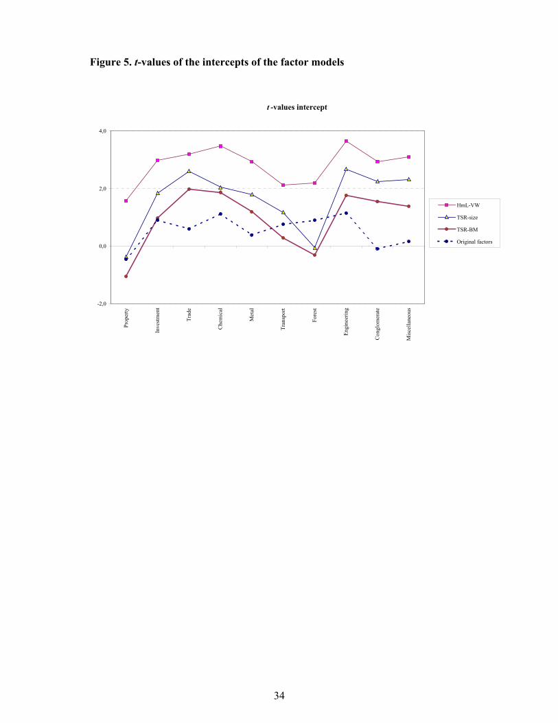
Finally we plot the intercept of the factor models and their t-values in Figure 4 and

Figure 5 respectively. The intercepts of the model with the TSR-size mimicking

portfolios are larger than that of the TSR-BM mimicking portfolios for all the

industries. They are also larger than the intercepts of the model with the original

factors for all but one industry. The intercept of the model with HmL-LW mimicking

portfolios due to the trivial impact of the market portfolio is extremely high.

Accordingly, the intercepts of this model are significant at the 5% level for all

industries except property. The model with TSR-size mimicking portfolios has also

five significant intercepts, while the other two models, i.e. models with the original

factors and TSR-BM, do not show any significant intercepts. These findings are in

accordance with the results of the likelihood ratio test in Table 5, which rejects the

TSR-size and HmL-LW models and does not rejects the two other models.

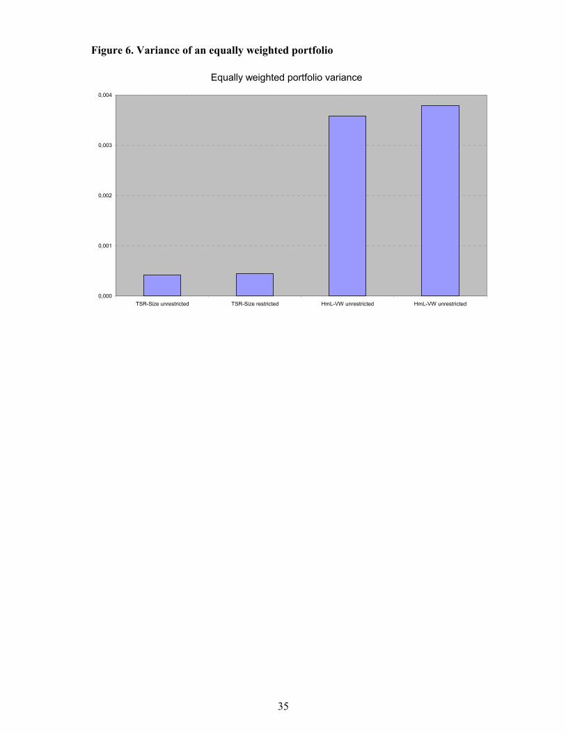
There is however one puzzle in the results of the likelihood ratio test, i.e. why the

p-value of the model based on the TSR-size is lower than that of the HmL-LW based

model, while according to the t-values we expect an opposing result. The motivation

is that the weakness of the factor model according to the HmL-LW portfolios not only

results in higher intercepts but at the same time gives a very large residual covariance

matrix, which is due to the unexplained components of the return covariations. This

larger covariance matrix increases the uncertainty of any type of the joint test. (See

MacKinlay, 1995, for the poor results of the joint F-test when there is a missing risk

factor in the model.) Figure 6 compares the magnitude of the residual covariance

matrices of these two models by forming an equally weighted portfolio based on these

covariance matrices. As expected the variance of the portfolios based on the

HmL-LW are extremely larger than those for the TSR-size based models.

6 Conclusions

In this paper we have investigated the ability of different factor mimicking portfolios

in representing the background factors. We apply several methods for constructing the

mimicking portfolios, i.e. the cross-sectional regression approach, the portfolio

approach and the time-series regression approach. We build two different CSR

18

mimicking portfolios that differ in the way we normalise the explanatory variables.

We use three different weighting methods for the portfolio approach and three

different types of the based assets to construct TSR mimicking portfolios.

In addition to the analysis of the standard deviations, the estimated factor risk premia

and the correlations between the mimicking portfolios we compare the mimicking

portfolios using an asset pricing model. The model is meant to explain the mean

excess returns of the Swedish industrial portfolios. The estimation results are

compared with the results of the model when the factors are represented by their

original realisation.

We find that the result of the portfolio approach is sensitive to the choice of the

weighting methods. However, the cross sectional regression approach gives almost

the same mimicking portfolio as the loading weighted portfolio approach. The value

weighted approach has a very little similarity with other methods. One important

finding is that the book-to-market is the only variable with significant mean return of

the cross-sectional mimicking portfolios. We find also that the choice of the based

assets is important for the estimated mimicking portfolios by the time series approach.

In contrast to the CSR- and the portfolio approach all the TSR mimicking portfolios

shows a highly significant mean excess return for the market.

In the asset pricing analysis, the models with the original factors and the model with

time-series mimicking portfolios, with the book-to-market sorted portfolios as the

base assets, outperform the other models.

As MacKinlay (1995) showed the joint F-test would be poor in rejecting a factor

model when there is a missing risk factor. Our likelihood ratio test for the model

including HmL-LW mimicking portfolios supports this hypothesis and shows that a

very weak factor model not only results in higher intercepts but at the same time gives

a very large residual covariance matrix. The latter is due the unexplained components

of the return covariations. The larger covariance matrix increases the uncertainty of

the tests and results in a higher p-value, which make it difficult to reject a bad factor

model.

In summary, based on the results from the asset pricing tests, we conclude that the

time series regression approach is a more proper way of constructing mimicking

portfolios than the other alternatives investigated in this paper. For our data the book-

19

to-market ratio, due to its relation to cross-sectional differences in mean returns,

found to be an appropriate candidate to construct the base assets for the time series

regression approach. However, the time series approach cannot be employed to

construct mimicking portfolios based on the firm characteristics, when the original

factors are not observed. In this case our suggestion is to use loading weighted

portfolio approach. The motivation is that despite the close relation between this

method and the theoretically motivated cross-sectional approach, the loading

weighted portfolio approach suffer less than the cross-sectional approach from

problems such as error in variables and normalising effects.

20

References

Breeden D. T., M. R. Gibbons, and R. H. Litzenberger, 1989, Empirical Tests of the

Consumption-Oriented CAPM, Journal of Finance 44, 231-262.

Chan, L. K. C., J. Karceski, and J. Lakonishok, 1998, The risk and return from

factors, Journal of Financial and Quantitative Analysis 33, 159-188.

Chan, L. K. C., J. Karceski, and J. Lakonishok, 1999, On portfolio optimization:

Forecasting covariances and choosing the risk model, The Review of Financial Studies

12, 937-974.

Cochrane, J. H., 2001, Asset pricing, Princeton, Princeton University Press.

Fama, E. F., 1976, Foundations of Finance, Basic Books, New York.

Fama, E. F. and K. R. French, 1993, Common Risk Factors in the Returns on Stocks

and Bonds, Journal of Financial Economics 33, 3-56.

MacKinlay, A. C., 1995, Multifactor Models Do Not Explain Deviations from the

CAPM, Journal of Financial Economics, 38, 3-28.

Vassalou, M., 2000, News related to future GDP growth as a risk factor in equity

returns, Journal of Financial Economics, forthcoming.

21

Table 1. Correlation between mimicking portfolios constructed by the univariate

CSR approach and the portfolio approach

The table reports the correlations between different factor mimicking portfolios that areconstructed by the univariate CSR approach and the portfolio approach. All the loadings areestimated by the univariate regression on 36 months overlapping windows. In the rankapproach, the explanatory variable is constructed by ranking all the loadings and normalisingthem between 0 and 2. In the distance approach, the explanatory variable is constructed bytaking into account the relative distances among the loadings. HmL refers to the mimickingportfolio constructed by the portfolio approach. EW, weighting all stocks equally. VWweighting all stocks by their relative market value. LW, and weighting all stocks by theirrelative loadings.

Method Method Market DIP Slope DEX Size BtoM AverageCSR-rank CSR-distance 0,98 0,95 0,96 0,97 0,85 0,89 0,93

HmL-VW 0,61 0,34 0,61 0,62 0,80 0,62 0,60HmL-EW 0,94 0,88 0,94 0,94 0,91 0,92 0,92

HmL-LW 0,98 0,95 0,96 0,97 0,93 0,94 0,95CSR-distance HmL-VW 0,59 0,21 0,51 0,58 0,90 0,54 0,56

HmL-EW 0,90 0,76 0,86 0,88 0,76 0,75 0,82 HmL-LW 0,99 0,97 0,98 0,99 0,94 0,98 0,97HmL-VW HmL-EW 0,66 0,53 0,67 0,64 0,87 0,64 0,67 HmL-LW 0,60 0,27 0,52 0,56 0,91 0,60 0,58HmL-VW HmL-LW 0,91 0,79 0,89 0,89 0,91 0,82 0,87

22

Table 2. Statistics of the mimicking portfolios constructed by the univariate CSR

approach and the portfolio approach

The table reports means, standard deviations and t-statistics of the factor mimicking portfoliosthat are constructed by the univariate CSR approach and the portfolio approach. All theloadings are estimated by the univariate regression on 36 months overlapping windows. In therank approach, the explanatory variable is constructed by ranking all the loadings andnormalising them between 0 and 2. In the distance approach, the explanatory variable isconstructed by taking into account the relative distances among the loadings. HmL refers tothe mimicking portfolio constructed by the portfolio approach. EW, weighting all stocksequally. VW weighting all stocks by their relative market value. LW, and weighting allstocks by their relative loadings.

Methods Market DIP Slope DEX Size BMMean annual CSR-rank 0,003 -0,006 0,019 0,002 -0,002 0,060

CSR-distance 0,000 -0,013 0,032 0,007 0,009 0,098HmL-VW 0,009 -0,020 0,036 0,020 0,026 0,045HmL-EW 0,001 -0,013 0,016 0,000 0,011 0,062HmL-LW 0,006 -0,011 0,030 0,006 0,015 0,093

Std annual CSR-rank 0,110 0,081 0,110 0,105 0,110 0,092CSR-distance 0,179 0,139 0,187 0,178 0,141 0,190HmL-VW 0,115 0,115 0,123 0,122 0,129 0,136HmL-EW 0,106 0,078 0,107 0,105 0,109 0,099HmL-LW 0,162 0,130 0,176 0,156 0,157 0,159

t-statistics CSR-rank 0,116 -0,31 0,70 0,08 -0,06 2,74**

CSR-distance 0,009 -0,39 0,72 0,15 0,27 2,15*

HmL-VW 0,327 -0,72 1,22 0,67 0,83 1,39HmL-EW 0,021 -0,72 0,63 0,01 0,41 2,62**

HmL-LW 0,143 -0,36 0,72 0,16 0,40 2,46*

23

Table 3. Correlation between mimicking portfolios constructed by the TSR

approach with different base portfolios

The table reports the correlations between the TSR mimicking portfolios and the originalseries. We use three alternative base assets: Ten size sorted portfolios, ten book-to-marketsorted portfolios and ten randomly sorted portfolios.

Size BM Random orig. seriesSize 1,00

Market BM 0,87 1,00 Random 0,79 0,82 1,00 orig. series 0,59 0,61 0,53 1,00 Size BM Random orig. seriesSize 1,00

DIP BM -0,23 1,00 Random 0,20 -0,12 1,00 orig. series 0,24 -0,19 0,22 1,00 Size BM Random orig. seriesSize 1,00

Slope BM 0,30 1,00 Random 0,29 0,12 1,00 orig. series 0,35 0,23 0,34 1,00 Size BM Random orig. seriesSize 1,00

DEX BM 0,67 1,00 Random 0,57 0,61 1,00 orig. series 0,35 0,37 0,36 1,00

24

Table 4. Statistics of the mimicking portfolios constructed by the TSR approach

with different base portfolios

The table reports the means, standard deviations and t-statistics of the TSR mimickingportfolios and the original series. We use three alternative base assets: Ten size sortedportfolios, ten book-to-market sorted portfolios and ten randomly sorted portfolios.

Market Sorting var. Size BM RandomAnnual mean 0,168 0,156 0,176Annual stdev 0,251 0,225 0,238t-test 2,81** 2,91** 3,09**

DIP Sorting var. Size BM RandomAnnual mean -0,068 -0,202 -0,009Annual stdev 0,812 2,637 0,808t-test -0,35 -0,32 -0,05

Slope Sorting var. Size BM RandomAnnual mean -0,139 -0,068 0,086Annual stdev 0,577 0,767 0,677t-test -1,01 -0,37 0,53

DEX Sorting var. Size BM RandomAnnual mean 0,234 0,215 0,173Annual stdev 0,310 0,308 0,354t-test 3,16** 2,92** 2,05*

25

Table 5. Likelihood ratio test

The table reports the result of the likelihood ratio tests. The null hypothesis is that all theintercepts are equal to zero.

Original factors TSR-size TSR-BM HmL-VWUnrestricted 3277,7 3584,4 3512,8 3291,2Restricted 3275,7 3574,2 3507,3 3281,6Likelihood ratio 3,88 20,58 11,16 19,23Degree of freedom 10 10 10 10P-value 0,95 0,02 0,35 0,04

26

Table 6. Multifactor asset pricing with the original factors

The table reports the estimated parameters of the unrestricted factor model with the originalfactors:

( ) ,1

it

K

kkktikmtimiit XRR εθββα +−++= ∑

=

kθ is the risk free part of the macroeconomic factors and are estimated within the model. Thetable also reports the risk premium associated with the factors.

Parameters of the unrestricted model with original macro variablesIndusty Intercept Market DIP Slope DEXProperty -0,003 0,902 0,369 0,007 0,361Investment 0,004 0,874 0,135 0,005 0,074Trade 0,004 0,671 0,350 0,005 -0,261Chemical 0,005 0,879 -0,011 -0,001 -0,258Metal 0,002 0,767 0,150 0,003 -0,289Transport 0,005 0,624 0,173 0,006 0,142Forest 0,005 0,826 0,084 0,003 0,303Engineering 0,005 0,891 0,097 0,002 -0,096Conglomerate 0,000 0,755 0,400 0,006 -0,327Miscellaneous 0,001 0,576 0,194 0,005 -0,225

Mean 0,011 0,003 0,482 0,004θk -0,013 0,449 0,012Risk premium 0,011 0,016 0,033 -0,009

27

Table 7. Multifactor asset pricing with the TSR-size mimicking portfolios

The table reports the estimated parameters of the unrestricted factor model when the factorsare represented by their TSR-size mimicking portfolios:

,1

1it

K

kktikiit RR εβα ++= ∑

+

=

The table also reports the risk premium associated with the factors.

Parameters of the model with TSR-size base Mimicking portfoliosIndusty Intercept Market DIP Slope DEXProperty -0,002 0,685 0,092 0,157 0,223Investment 0,004 1,036 0,013 0,118 -0,094Trade 0,012 0,930 0,024 0,116 -0,262Chemical 0,007 0,856 -0,048 0,011 -0,111Metal 0,006 1,066 0,015 0,080 -0,233Transport 0,005 0,756 0,081 0,178 0,009Forest 0,000 0,889 0,000 0,100 0,106Engineering 0,005 1,085 0,001 0,027 -0,140Conglomerate 0,009 0,970 0,041 0,127 -0,197Miscellaneous 0,006 0,828 0,041 0,068 -0,226

Risk premium 0,014 -0,006 -0,012 0,020

28

Table 8. Multifactor asset pricing with the TSR-BM mimicking portfolios

The table reports the estimated parameters of the unrestricted factor model when the factorsare represented by their TSR-BM mimicking portfolios:

,1

1it

K

kktikiit RR εβα ++= ∑

+

=

The table also reports the risk premium associated with the factors.

Parameters of the model with TSR-BM base Mimicking portfoliosIndusty Intercept Market DIP Slope DEXProperty -0,004 0,455 -0,013 0,131 0,498Investment 0,002 0,565 -0,009 0,102 0,359Trade 0,010 0,393 -0,018 0,084 0,239Chemical 0,006 1,052 0,021 -0,038 -0,134Metal 0,004 0,632 -0,022 0,074 0,174Transport 0,001 0,412 -0,023 0,077 0,369Forest -0,001 0,574 -0,025 0,060 0,382Engineering 0,005 0,727 -0,011 0,039 0,183Conglomerate 0,006 0,646 -0,016 0,093 0,148Miscellaneous 0,004 0,541 -0,015 0,048 0,079

Risk premium 0,013 -0,017 -0,006 0,018

29

Table 9. Multifactor asset pricing with the with HmL-LW Mimicking portfolios

The table reports the estimated parameters of the unrestricted factor model when the factorsare represented by their HmL-VW mimicking portfolios:

,1

1it

K

kktikiit RR εβα ++= ∑

+

=

The table also reports the risk premium associated with the factors.

Parameters of the model with CSR Mimicking portfoliosIndusty Intercept Market DIP Slope DEXProperty 0,009 0,331 0,386 0,585 0,362Investment 0,015 0,372 -0,060 0,216 0,285Trade 0,019 -0,037 0,062 0,015 0,215Chemical 0,017 0,336 0,033 -0,105 0,072Metal 0,015 0,252 -0,202 0,050 0,357Transport 0,012 0,113 0,111 0,280 0,438Forest 0,012 0,527 -0,153 0,149 0,264Engineering 0,017 0,681 -0,102 0,034 -0,051Conglomerate 0,017 0,101 -0,138 0,082 0,316Miscellaneous 0,012 0,076 0,061 -0,034 0,256

Risk premium 0,0005 -0,0009 0,0025 0,0005

30

Figure 1. Annual standard deviations of the mimicking portfolios constructed bythe univariate CSR approach and the portfolio approach

Annual standard deviation

0,000,020,040,060,080,100,120,140,160,180,20

Market DIP Slope DEX Size BM

HmL-VWHmL-EWHmL-LW

31

Figure 2. Factor exposure of the industrial portfolios

Market

-0,2

0,0

0,2

0,4

0,6

0,8

1,0

1,2

Prop

erty

Inve

stm

ent

Trad

e

Che

mic

al

Met

al

Tran

spor

t

Fore

st

Engi

neer

ing

Con

glom

erat

e

Mis

cella

neou

s

DIP

-0,3

-0,2

-0,1

0,0

0,1

0,2

0,3

0,4

0,5

Prop

erty

Inve

stm

ent

Trad

e

Che

mic

al

Met

al

Tran

spor

t

Fore

st

Engi

neer

ing

Con

glom

erat

e

Mis

cella

neou

s

Slope

-0,2

-0,1

0,0

0,1

0,2

0,3

0,4

0,5

0,6

0,7

Prop

erty

Inve

stm

ent

Trad

e

Che

mic

al

Met

al

Tran

spor

t

Fore

st

Engi

neer

ing

Con

glom

erat

e

Mis

cella

neou

s

DEX

-0,3

-0,2

-0,1

0,0

0,1

0,2

0,3

0,4

0,5

0,6

Prop

erty

Inve

stm

ent

Trad

e

Che

mic

al

Met

al

Tran

spor

t

Fore

st

Engi

neer

ing

Con

glom

erat

e

Mis

cella

neou

s

Original factors

TSR_size

TSR_BM

HmL-VW

32

Figure 3. Impact of the factor on mean excess returns given by different factormodels

Market

-0,002

0,002

0,006

0,010

0,014

Prop

erty

Inve

stm

ent

Trad

e

Che

mic

al

Met

al

Tran

spor

t

Fore

st

Engi

neer

ing

Con

glom

erat

e

Mis

cella

neou

s

Original factors

TSR_size

TSR_BM

HmL-LW

DIP

-0,002

0,000

0,002

0,004

0,006

0,008

Prop

erty

Inve

stm

ent

Trad

e

Che

mic

al

Met

al

Tran

spor

t

Fore

st

Engi

neer

ing

Con

glom

erat

e

Mis

cella

neou

s

Slope

-0,003

-0,002

-0,001

0,000

0,001

0,002

Prop

erty

Inve

stm

ent

Trad

e

Che

mic

al

Met

al

Tran

spor

t

Fore

st

Engi

neer

ing

Con

glom

erat

e

Mis

cella

neou

s

DEX

-0,008

-0,004

0,000

0,004

0,008

0,012

Prop

erty

Inve

stm

ent

Trad

e

Che

mic

al

Met

al

Tran

spor

t

Fore

st

Engi

neer

ing

Con

glom

erat

e

Mis

cella

neou

s

33

Figure 4. The intercept of the factor models

Intercept

-0,010

-0,005

0,000

0,005

0,010

0,015

0,020

Prop

erty

Inve

stm

ent

Trad

e

Che

mic

al

Met

al

Tran

spor

t

Fore

st

Engi

neer

ing

Con

glom

erat

e

Mis

cella

neou

s

Original factors

HmL-VW

TSR-size

TSR-BM

34

Figure 5. t-values of the intercepts of the factor models

t -values intercept

-2,0

0,0

2,0

4,0Pr

oper

ty

Inve

stm

ent

Trad

e

Che

mic

al

Met

al

Tran

spor

t

Fore

st

Engi

neer

ing

Con

glom

erat

e

Mis

cella

neou

s

HmL-VW

TSR-size

TSR-BM

Original factors

35

Figure 6. Variance of an equally weighted portfolio

0,000

0,001

0,002

0,003

0,004

TSR-Size unrestricted TSR-Size restricted HmL-VW unrestricted HmL-VW unrestricted

Equally weighted portfolio variance