A Comparative Evaluation of Techniques for StudyingParallel System Performance

�

Anand SivasubramaniamUmakishore Ramachandran

H. Venkateswaran

Technical Report GIT-CC-94/38September 1994

College of ComputingGeorgia Institute of Technology

Atlanta, GA 30332-0280Phone: (404) 894-5136

Fax: (404) 894-9442e-mail: rama@cc.gatech.edu

Abstract

This paper presents a comparative and qualitative survey of techniques for evaluating parallel systems. Wealso survey metrics that have been proposed for capturing and quantifying the details of complex parallel systeminteractions. Experimentation, theoretical/analytical modeling and simulation are three frequently used techniques inperformance evaluation. Experimentation uses real or synthetic workloads, usually called benchmarks, to measureand analyze their performance on actual hardware. Theoretical and analytical models are used to abstract details of aparallel system, providing the view of a simplified system parameterized by a limited number of degrees of freedomthat are kept tractable. Simulation and related performance monitoring/visualization tools have become extremelypopular becauseof their ability to capture the dynamic nature of the interaction between applications and architectures.We first present the figures of merit that are important for any performance evaluation technique. With respect tothese figures of merit, we survey the three techniques and make a qualitative comparison of their pros and cons.In particular, for each of the above techniques we discuss: representative case studies; the underlying models thatare used for the workload and the architecture; the feasibility and ease of quantifying standard performance metricsfrom the available statistics; the accuracy/validity of the output statistics; and the cost/effort that is expended in eachevaluation strategy.

Key Words: Parallel systems, performance metrics, performance evaluation, experimentation, theoretical/analyticalmodels, simulation.

�This work has been funded in part by NSF grants MIPS-9058430 and MIPS-9200005, and an equipment grant from DEC.

1 Introduction

Evaluating and analyzing the performance of a parallel application on an architecture is an important aspect of parallel

systems1 research. Such a performance study may be used to: select the best architecture platform for an application

domain, select the best algorithm for solving the problem on a given hardware platform, predict the performance

of an application on a larger configuration of an existing architecture, predict the performance of large application

instances, identify application and architectural bottlenecks in a parallel system to suggest application restructuring and

architectural enhancements, and glean insight on the interaction between an application and an architecture to predict

the performance of other application-architecture pairs. But evaluating and analyzing parallel system performance

is hard due to the complex interaction between application characteristics and architectural features. Performance

evaluation techniques have to grapple with several more degrees of freedom exhibited by these systems relative to their

sequential counterparts. In this paper, we conduct a comparative and qualitative survey of performance evaluation

techniques, using figures of merit to bring out their pros and cons.

The performance of a parallel system can be quantified using a set of metrics. For an evaluation technique to be

useful it should provide the necessary set of metrics needed for understanding the behavior of the system. Hence,

to qualify any evaluation technique, we need to identify a desirable set of metrics and investigate the capabilities of

the technique in providing these metrics. We present metrics that have been proposed for quantifying parallel system

performance, discussing the amount of information provided by each towards a detailed understanding of the behavior

of the system.

We review the techniques used in performance evaluation,namely, experimentation, theoretical/analytical modeling

and simulation. Experimentation uses real or synthetic workloads, usually called benchmarks, to measure and analyze

their performance on actual hardware. Theoretical and analytical models are used to abstract details of a parallel

system, providing the view of a simplified system parameterized by a limited number of degrees of freedom that are

kept tractable. Simulation is a useful modeling and monitoring technique that has become extremely popular because

of its ability to capture the complex and dynamic nature of the interaction between applications and architecture in a

non-intrusive manner. For each technique, we illustrate the methodology used with examples. We present some of the

input models that each technique uses, and compare the techniques based on the output statistics, the accuracy of these

statistics, and the cost/effort expended. We also briefly describe some of the tools that have been built embodying

these techniques.

In Section 2, we identify several desirable metrics that have been proposed by researchers. Section 3 gives a

framework that we use for comparing these techniques, identifying some figures of merit. In Sections 4, 5 and

6, we discuss the pros and cons of experimentation, theoretical/analytical modeling and simulation respectively, in

terms of the above-mentioned figures of merit. We also identify some of the tools that have been developed using

each technique to help evaluate parallel systems. Section 7 summarizes the results of our comparison and outlines

an evaluation strategy that combines the merits of the three techniques while avoiding some of their drawbacks and

Section 8 presents concluding remarks.

1The term, parallel system, is used to denote an application-architecture combination.

2 Metrics

In evaluating a system, we need to identify a set of performance metrics that provide adequate information to understand

the behavior of the system. Metrics which capture the processor characteristics in terms of the clock speed (MHz), the

instruction execution speed (MIPS), the floating point performance (MFLOPS), and the execution time for standard

benchmarks (SPEC) have been widely used in modeling uniprocessor performance. A nice property of a uniprocessor

system is that given the hardware specifications it is fairly straightforward to predict the performance for any application

to be run on the system. However, in a parallel system the hardware specification (which quantifies the available

compute power) may never be a true indicator of the performance delivered by the system. This is due to the growth

of overheads in the parallel system either because of the application characteristics or certain architectural limitations.

Metrics for parallel system performance evaluation should quantify this gap between available and delivered compute

power. Scalability is a notion that is frequently used to express the disparity between the two, in terms of the match

between an application and an architecture. Metrics proposed for scalability attempt to quantify this match. We

summarize some of the proposed metrics in this section and also discuss the amount of information provided by each

metric towards understanding the parallel system execution. The reader is referred to [33] for a detailed survey of

different performance metrics for scalability.

Speedup is a widely used metric for quantifying improvements in parallel system performance as the number of

processors is increased. Speedup(p) is defined as the ratio of the time taken by an application of fixed size to execute

on one processor to the time taken for executing the same on � processors. Parallel computers promise the following

enhancements over their sequential counterparts, each of which leads to a corresponding scaling strategy: 1) the number

of processing elements is increased enabling a potential performance improvement for the same problem (constant

problem size scaling); 2) other system resources like primary and secondary storage are also increased enhancing the

capability to solve larger problems (memory-constrained scaling); 3) due to the larger number of processing elements,

a much larger problem may be solved in the same time it takes to solve a smaller problem on a sequential machine

(time-constrained scaling). Speedup captures only the constant problem size scaling strategy. It is well known that

for a problem with a fixed size, the maximum possible speedup with increasing number of processors is limited by the

serial fraction in the application [4]. But very often, parallel computers are used for solving larger problems and in

many of these cases the sequential portion of the application may not increase appreciably regardless of the problem

size [30] yielding a lower serial fraction for larger problems. In such cases, memory-constrained and time-constrained

scaling strategies are more useful. Gustafson et al. [30] introduce a metric called scaled-speedup that tries to capture

the memory-constrained scaling strategy. Scaled speedup is defined as the speedup curve obtained when the problem

size is increased linearly with the number of processors. Sun and Gustafson [58] propose a metric called sizeup to

capture the time-constrained scaling strategy. Sizeup is defined as the ratio of the size of the problem solved on the

parallel machine to the size of the problem solved on the sequential machine for the same execution time.

When the execution time does not decrease linearly with the number of processors, speedup does not provide any

additional information needed to find out if the deviation is due to bottlenecks in the application or in the machine.

Similarly, when a parallel system exhibits non-ideal behavior in the memory-constrained or time-constrained scaling

2

strategies, scaled-speedup and sizeup fail to show whether the problem rests with the application and/or the architecture.

Three other metrics [34, 32, 43] attempt to address this deficiency. Isoefficiency function [34] tries to capture the impact

of problem sizes along the application dimension and the number of processors along the architectural dimension. For

a problem with a fixed size, the processor utilization (efficiency) normally decreases with an increase in the number of

processors. Similarly, if we scale up the problem size keeping the number of processors fixed, the efficiency usually

increases. Isoefficiency function relates these two artifacts in typical parallel systems and is defined as the rate at

which the problem size needs to grow with respect to the number of processors inorder to keep the efficiency constant.

An isoefficiency whose growth is faster than linear suggests that overheads in the hardware are a limiting factor in the

scalability of the system, while a growth that is linear or less is indicative of a more scalable hardware. Apart from

providing a bound on achievable performance (Amdahl’s law), the theoretical serial fraction of an application is not

very useful in giving a realistic estimate of performance on actual hardware. Karp and Flatt [32] use an experimentally

determined serial fraction � for a problem with a fixed size in evaluating parallel systems. � is computed by executing

the application on the actual hardware and calculating the effective loss in speedup. On an ideal architecture with no

overheads introduced by the hardware, � would be equal to the theoretical serial fraction of the application. Hardware

deficiencies lead to a higher � and a constant � with increasing number of processors implies a scalable parallel system

very often suggesting that there is no overhead introduced by the underlying hardware. Decreasing � is an indication

of superlinear speedup that arises due to reasons such as memory size and randomness in application execution, as

outlined in [31]. Nussbaum and Agarwal [43] quantify scalability as a ratio of the application’s asymptotic speedup

when run on the actual architecture to its corresponding asymptotic speedup when run on an EREW PRAM [26], for a

given problem size. Application scalability is a measure of the inherent parallelism in the application and is expressed

by its speedup on an architecture with an idealized communication structure such as a PRAM. Architectural scalability

is defined as the relative performance between the ideal and real architectures. A larger ratio is an indication of better

performance obtained in running the given application on the hardware platform.

Metrics used by [34, 32, 43] thus attempt to identify the cause (the application or the architecture) of the problem

when the parallel system does not scale as expected. Once the problem is identified, it is essential to find the individual

application and architectural artifacts that lead to these bottlenecks and to quantify their relative contribution towards

limiting the overall scalability of the system. For instance, we would like to find the contribution of the serial portion

in the application, the work-imbalance between the threads of control in the program, the overheads introduced by

parallelization of the problem, towards limiting the scalability of the application. Similarly, it would be desirable to

quantify the contribution from hardware components such as network latency, contention, and synchronization, and

system software components such as scheduling and other runtime overheads. But it is difficult to glean this knowledge

from the three metrics. Identifying, isolating and quantifying the different overheads in a parallel system that limit

its scalability is crucial for improving the performance of the system by application restructuring and architectural

enhancements. It can also help in choosing between alternate application implementations, selecting the best hardware

platform, and the different other uses of a performance analysis study outlined earlier in section 1. Recognizing this

importance, studies [57, 56, 16, 13] have attempted to separate and quantify parallel system overheads.

3

Linear

Actual

Processors

Spee

dup

AlgorithmicOverheads

SoftwareInteractionOverheads

HardwareInteractionOverheads

Figure 1: Overheads in a Parallel System

Ignoring effects of superlinearity, one would expect a speedup that increases linearly with the number of processors,

as shown by the curve named “linear” in Figure 1. But overheads in the system would limit its scalability resulting

in a speedup that grows much slower as shown by the curve labelled “actual” in Figure 1. The disparity between

the “linear” and “actual” curves is due to growth of overheads in the parallel system. Parallel system overheads

may be broadly classified into a purely algorithmic component (algorithmic overhead), a component arising from

the interaction of the application with the system software (software interaction overhead), and a component arising

from the interaction of the application with the hardware (hardware interaction overhead). Algorithmic overheads

arise from the inherent serial part in the application, the work-imbalance between the executing threads of control,

any redundant computation that may be performed, and additional work introduced by the parallelization. Software

interaction overheads such as overheads for scheduling, message-passing, and software synchronization arise due to the

interaction of the application with the system software. Hardware slowdown due to network latency (the transmission

time for a message in the network), network contention (the amount of time spent in the network waiting for links to

become free), synchronization and cache coherence actions, contribute to the hardware interaction overhead. To fully

understand the scalability of the parallel system, it is important to isolate and quantify the impact of different parallel

system overheads on the overall execution as shown in Figure 1. Overhead functions [56, 57] and lost cycles [16] are

metrics that have been proposed to capture the growth of overheads in a parallel system. Both these metrics quantify

the contribution of each overhead towards the overall execution time. The studies differ in the techniques used to

quantify these metrics. Experimentation is used in [16] to quantify lost cycles, while simulation is used in [56, 57] to

quantify overhead functions.

In addition to quantifying the overheads in a given parallel system, a performance evaluation technique should

also be able to quantify the growth of overheads as a function of system parameters such as problem size, number of

processors, processor clock speed, and network speed. This information can prove useful in predicting the scalability

4

of systems governed by a different set of parameters.

In this section, we presented a range of performance metrics, from simple metrics like speedup which provide

scalar information about the performance of the system, to more complicated vector metrics like overhead functions

that provide a wide range of statistics about the parallel system execution (see Table 1). The metrics that reveal only

scalar information are much easier to calculate. In fact, the overall execution times of the parallel system parameterized

by number of processors and problem sizes would suffice to calculate metrics like speedup, scaled speedup, sizeup,

isoefficiency function and experimentally determined serial fraction. On the other hand, the measurement of overhead

functions and lost cycles would need more sophisticated techniques that use a considerable amount of instrumentation.

Metrics Merits Drawbacks

Speedup, Scaled speedup,Sizeup

Useful for quantifying perfor-mance improvements as a func-tion of the number of processorsand problem sizes.

Do not identify or quantify bot-tlenecks in the system, provid-ing no additional informationwhen the system does not scaleas expected.

Isoefficiency function, Experi-mentally determined serial frac-tion, Nussbaum and Agarwal’smetric

Attempt to identify if the appli-cation or architecture is at faultin limiting the scalability of thesystem.

The information provided maynot be adequate to identify andquantify the individual applica-tion and architectural featuresthat limit the scalability of thesystem.

Overhead functions, Lost cycles

Identify and quantify all the ap-plication and architectural over-heads in a parallel system thatlimit its scalability, providing adetailed understanding of paral-lel system behavior.

Quantification of these metricsneeds more sophisticated instru-mentation techniques.

Table 1: Performance Metrics

3 The Framework

For each of the three techniques reviewed in this paper, we present an overview, illustrating its use with case-studies.

Evaluation studies using these techniques may be broadly classified into two categories: those which study the

performance of the system as a whole, and those which study the performance and scalability of specific system

artifacts such as locality properties, synchronization primitives, interconnection networks, and scheduling strategies.

We present examples from both categories.

Each evaluation technique uses an input model for abstracting the application and hardware characteristics in the

parallel system being evaluated. For instance, the abstraction for the machine can vary from the actual hardware as

is the case with experimentation, to a completely abstract model such as the PRAM [26]. Similarly, the application

model can range from a completely synthetic workload to a full-fledged application. We present models used in the

evaluation techniques and discuss the realism in these models in capturing the behavior of actual parallel systems.

The figures of merit used to compare the three techniques are as follows:

5

� Statistics examines the capabilities of the technique towards providing the desirable metrics identified in section

2. As we observed earlier, the overall execution time, which is provided by all three evaluation techniques,

would suffice to calculate the scalar metrics. On the other hand, isolation of parallel system overheads may not

be easily handled by a technique that is inherently limited by the amount of statistics it provides.

We also discuss the capability of the technique towards studying the impact of application parameters such as

problem size, and hardware parameters such as number of processors, CPU clock speed, and network bandwidth,

on system performance. We can vary these system parameters and re-conduct the evaluation to investigate their

impact on the performance metric being studied. These results, coupled with knowledge about the application

and hardware, can be used to develop analytical and regression models of system performance. Such models

can identify bottlenecks in the system and help predict the scalability of parallel systems governed by a different

set of parameters.

� Accuracy evaluates the validity and reliability of the results from the technique. Intrinsic and external factors

determine the accuracy of an evaluation. To a large extent, the accuracy depends on intrinsic factors such as the

closeness of the chosen input models to the actual system. The accuracy may also depend on external factors

such as monitoring and instrumentation. Even the act of measurement may sometimes perturb the accuracy of

the evaluation.

� We investigate the cost and effort expended in each evaluation strategy in terms of computer and human

resources. We study the initial cost expended in developing the input models, and the subsequent cost for the

actual evaluation. These two costs may also be used to address the capability of the technique towards handling

modifications to the parallel system. A slight change of system parameters, which do not alter the input model,

would demand only an evaluation cost. On the other hand, more drastic changes to the application and/or the

hardware would also incur the cost of re-designing the input models.

4 Experimentation

4.1 Overview

The experimentation technique for evaluating parallel systems uses real or synthetic workloads and measures their

performance on actual hardware. For instance, several studies [22, 11, 47, 49] experiment with the KSR-1 hardware for

evaluating its computation, communication and scalability properties. The scalability of the KSR-1 is studied in [47]

using applications drawn from the NAS benchmark suite [9]. Similarly, an experimental evaluation of the computation

and communication capabilities of the CM-5 is conducted in [46]. Lenoski et al. [36] evaluate the scalability of

the Stanford DASH multiprocessor prototype using a set of applications. These applications are implemented on

the prototype hardware and their performance is studied using a hardware monitor to obtain statistics on processor

usage, cache statistics and network traffic. The statistics are used to explain the deviation of application performance

from ideal behavior. Such evaluations of machine performance using benchmarks may be used to compare different

6

hardware platforms. Singh et al. [52] thus use applications from the SPLASH benchmark suite [54] to compare the

KSR-1 and DASH multiprocessors.

Experimentation has also been used to study the performance and scalability of specific system artifacts such

as locality, synchronization, and interconnection network. The interconnection network and locality properties of

the KSR-1 are studied in [22, 11, 49]. Lenoski et al. [36] study the performance and scalability of the cache,

synchronization primitives and the interconnection network of DASH. They implement artificial workloads which

exercise different synchronization alternatives and the prefetch capabilities of the DASH prototype, and measure their

performance as a function of the number of processors. The scalability of hardware and software synchronization

primitives on the Sequent Symmetry and BBN Butterfly hardware platforms is investigated in [41] and [5]. In these

studies, each processor is subjected to a large number of synchronization operations to calculate the average overhead

for a single operation. The growth of this overhead as a function of the number of processors is used as a measure of

the scalability of the synchronization primitive.

4.2 Input Model

Experimentation uses the actual hardware and the related system software to conduct the evaluation, making it the

most realistic model from the architectural point of view. On the other hand, the workload model (often called

benchmarks) used in evaluations can span a diverse spectrum of realism. The simplest benchmarks exercise and

measure the performance of low-level hardware features. Workloads used in [22] and [46] which evaluate the low-level

communication performance of the KSR-1 and CM-5 respectively, are examples of such benchmarks. The workload

used in [46] evaluates the performance of the CM-5 network by inducing messages to traverse different levels of

the fat-tree network under a variety of traffic conditions. Synthetic benchmarks that mimic the behavior of some

applications have also been used for evaluating systems. Boyd et al. [11] propose a synthetic benchmark using sparse

matrices that is expected to model the behavior of typical sparse matrix computations. Synthetic benchmarks called

micro-kernels are used in [49] to evaluate the KSR-1. Varying parameters in these synthetic benchmarks is expected to

capture typical workloads of real applications. Another common way of benchmarking and studying system artifacts

is by experimenting with well-known parallel algorithms. Three such frequently used text book algorithms are used in

[55] to evaluate the performance of two shared memory multiprocessors, and to study the impact of task granularity,

data distribution and scheduling strategies on system performance.

Benchmarking using low-level measurements, and synthetic workloads has often been criticized due to the lack

of realism in capturing the behavior of real applications. Since applications set the standards for computing, it is

appropriate to use real-world applications for the performance evaluation of parallel machines, adhering to the RISC

ideology in the evolution of sequential architectures. Application suites such as the Perfect Club [10], the NAS

Parallel Benchmarks [9], and the SPLASH application suite [54] have been proposed for the evaluation of parallel

machines. However, applications normally tend to contain large volumes of code that are not easily portable, and

a level of detail that is not very familiar to someone outside that application domain. Hence, computer scientists

have traditionally used abstractions that capture the interesting computation phases of applications for benchmarking

7

their machines. Such abstractions of real applications which capture the main phases of the computation are called

kernels. One can go even lower than kernels by abstracting the main loops in the computation (like the Lawrence

Livermore loops [39]) and evaluating their performance. As one goes lower, the outcome of the evaluation becomes

less realistic. Even though an application may be abstracted by the kernels inside it, the sum of the times spent in

the underlying kernels may not necessarily yield the time taken by the application. There is usually a cost involved

in moving from one kernel to another such as the data movements and rearrangements in an application that are

not part of the kernels that it is comprised of. For instance, an efficient implementation of a kernel may need to

have the input data organized in a certain fashion which may not necessarily be the format of the output from the

preceding kernel in the application. Despite these drawbacks, kernels may still be used to give a reasonable estimate of

application performance in circumstances where the cost of implementing and evaluating the entire application has to

be minimized. However, there are no inherent drawbacks in the experimentation technique that preclude implementing

the complete details of a real-world application. The technique thus benefits from the realism of the input model, both

from the hardware and the application point of view, giving credibility to results drawn from the evaluation.

4.3 Figures of Merit

4.3.1 Statistics

Experimentation can give the overall execution time of the application on the specified hardware platform. Conducting

the evaluation with different problem sizes and number of processors would thus suffice to calculate metrics such as

speedup, scaled speedup, sizeup, isoefficiency, and experimentally determined serial fraction identified in section 2.

But the overall execution time is not adequate to isolate and quantify parallel system overheads, and experimentation

needs to provide additional information. Two ways of acquiring such information is by instrumentation and hardware

monitoring. Instrumentation augments the application code or the system software to accumulate statistics about the

program execution. This augmentation may be performed either by the application programmer by hand, or may be

relegated to a pre-processor or even the compiler. Crovella and LeBlanc [16] identify such a tool called predicate

profiler, which uses a run-time library to log events from the application code to find algorithmic overheads such as

serial part and work-imbalance. A detailed analysis of the execution time would require a considerable amount of

instrumentation of the application code. In some cases, such detailed instrumentation may itself become intrusive,

yielding inaccurate results. Also, it is difficult to capture hardware artifacts such as network traffic and cache actions

by a simple instrumentation of the application. Hardware monitoring tries to remedy the latter deficiency by using

hardware support to accumulate these statistics. The hardware facilities on the KSR-1 for monitoring network traffic

and cache actions are used in [16] to calculate hardware interaction overheads such as network latency and contention.

But the hardware monitoring technique relies on support from the underlying hardware for accumulating statistics

and such facilities may not be available uniformly across all hardware platforms. Further, hardware monitoring alone

cannot give sufficient information about algorithmic and software interaction overheads. A combination of application

instrumentation and hardware monitoring may be used to remedy some of these problems. But the strategy would still

suffer from the intrusive nature of the instrumentation in interfering with both the algorithmic and hardware monitoring

8

mechanisms.

As we mentioned in section 3, we would like to vary application and hardware parameters and study their impact on

system performance. Application parameters such as problem size, may be easily studied with little or no modifications

to the application code, since most programs are likely to be written parameterized by these values. From the hardware

point of view, the number of processors can be varied. Also, some machines provide flexibility in hardware capabilities,

like the ability to vary the cache coherence protocol on the FLASH [35] multiprocessor. For such parameters, one

may be able to vary the hardware capabilities and develop analytical or regression models for predicting their impact

on performance. Crovella and LeBlanc [16] use such an approach to develop analytical models parameterized by the

problem size and the number of processors for the lost cycles of FFT on the KSR-1. But several other features in the

underlying hardware, such as the processing and network speed, are fixed, making it infeasible to study their impact

on system scalability.

4.3.2 Accuracy

Experimentation can use real applications to conduct the evaluation on actual machines giving accurate results with

respect to factors intrinsic to the system. But, as we observed earlier, it may be necessary to augment the experimentation

technique in order to obtain sufficient execution statistics. Such external instrumentation and monitoring intrusion can

perturb the accuracy of results.

4.3.3 Cost/Effort

The cost in developing the input model for experimentation is the effort expended in developing algorithms for the

given application, arriving at a suitable implementation which is optimized for the given hardware, and debugging

the resulting code. This cost is directly dependent on the complexity of the application and would be incurred in any

case since the application would ultimately need to be implemented for the given hardware. Further, this cost can be

amortized in conducting the evaluations over a range of hardware platforms and a range of application parameters with

little modifications to the application code. The cost for conducting the actual evaluation is the execution time of the

given application, which may be considered reasonable since the execution is on the native parallel hardware.

Modifications to the application and hardware can thus be accommodated by the experimentation technique at

a modest cost. Modifications to the application would involve recompiling the application and re-conducting the

evaluation. When the underlying hardware is changed, re-compilation and re-evaluation would normally suffice. A

drastic change in the hardware may sometimes lead to a change in the application code for performance reasons, or

may even change the programming paradigm used. But such cases are expected to be rare given that parallel machine

abstractions are rapidly converging from the user’s viewpoint.

4.4 Tools

Tools which use experimentation for performance debugging of parallel programs rely on the above-mentioned

instrumentation and hardware monitoring techniques for giving additional information about parallel system execution.

9

Quartz [6] uses instrumentation to give a profile of the time spent in different sections of the parallel program similar

to the Unix utility called ‘gprof’ which is frequently used in performance debugging of sequential programs. Quartz

provides a metric called normalized execution time which is defined as the total processor time spent in each section

of code divided by the number of processors that are concurrently busy when that section of code is being executed.

Such a tool can help in identifying bottlenecks in sections of code, but it is difficult to understand the reason for

such bottlenecks without the separation of the different parallel system overheads. Mtool [28] is another utility which

uses instrumentation to give additional information about the execution. In the first step, Mtool instruments the basic

blocks in the program and creates a performance profile. From this profile, it identifies important regions in the

code to instrument further with performance probes. The resulting code is re-executed to accumulate statistics such

as the time spent by a processor performing work (compute time), the time a processor is stalled waiting for data

(memory overhead), the time spent waiting at synchronization events (synchronization overhead), and the time spent

in performing work not present in the sequential code (additional work due to parallelization). IPS-2 [42] also uses

instrumentation to analyze parallel program performance. It differs from Quartz and Mtool in that it generates a trace

of events during application execution, and then analyzes the trace to present useful information to the user. Apart

from giving information like those provided by Mtool, the traces can also help determine dynamic interprocessor

dependencies. On the other hand, the generation of traces tends to increase the intrusiveness of instrumentation apart

from generating large trace files.

Instrumentation can help in identifying and quantifying algorithmic overheads, but it is difficult to quantify the

hardware interaction overheads using this technique alone. Hardware monitoring can supplement instrumentation to

remedy this problem. Burkhart and Millen [13] identify a set of hardware and system software monitoring tools that

help them quantify several sources of parallel system overheads on the M3 multiprocessor system. Software agents

called the ‘trap monitor’ and the ‘mailbox monitor’ are used to quantify algorithmic and synchronization overheads.

The ‘bus count monitor’, a hardware agent, is used to analyze overheads due to the network. Crovella and LeBlanc

[16] use a Lost Cycle Analyzer (LCA) to quantify parallel system overheads on the KSR-1. LCA uses instrumentation

to track performance loss resulting from algorithmic factors such as work-imbalance and serial parts in the program.

Appropriate calls to library functions are inserted in the application code to accumulate these statistics. LCA also uses

the KSR-1 network monitoring support, which can give the total time taken by each message, to calculate performance

loss in terms of the network latency and contention components.

The above tools are general purpose since they may be used to study any application on the given hardware

platform. Tools that are tailored to specific application domains have also been developed. For instance, SHMAP [21]

has been developed to aid in the design and understanding of matrix problems. Like IPS-2, it generates traces from

instrumented FORTRAN programs which are subsequently animated. While such a tool may not identify and quantify

all sources of overheads in the system, it can help in studying the memory access pattern of matrix applications towards

understanding its behavior with different memory hierarchies and caching strategies.

10

5 Theoretical/Analytical Models

5.1 Overview

As we observed early in this paper, performance evaluation of parallel systems is hard owing to the several degrees of

freedom that they exhibit. Analytical and theoretical models try to abstract details of a system, in order to limit these

degrees of freedom to a tractable level. Such abstractions have been used for developing parallel algorithms and for

performance analysis of parallel systems.

Abstracting machine features by theoretical models like the PRAM [26] has facilitated algorithm development and

analysis. These models try to hide hardware details from the programmer, providing a simplified view of the machine.

The utility of such models towards developing efficient algorithms for actual machines, depends on the closeness of

the model to the actual machine. Several machine models [2, 3, 27, 14, 59, 17] have been proposed over the years

to bridge the gap between the theoretical abstractions and the hardware. But, a complex model that incorporates all

the hardware details would no longer limit the degrees of freedom to a tractable level, precluding its ease of use for

algorithm development and analysis. Hence, research has focussed on developing simple models that incorporate a

minimal set of parameters which are important from a performance point of view. The execution time of applications

is expressed as a function of these parameters.

While theoretical models attempt to simplify hardware details, analytical models abstract both the hardware and

application details in a parallel system. Analytical models capture complex system features by simple mathematical

formulae, parameterized by a limited number of degrees of freedom that are tractable. Such models have found more

use in performance analysis than in algorithm development where theoretical models are more widely used. As with

experimentation, analytical models have been used to evaluate overall system performance as well as the performance

of specific system artifacts. Vrsalovic et al. [62] develop an analytical model for predicting the performance of

iterative algorithms on a simple multiprocessor abstraction, and study the impact of the speed of processors, memory,

and network on overall performance. Similarly, [37] studies the performance of synchronous parallel algorithms with

regular structures. The restriction to regular iterative and synchronous behavior of the application in these studies

helps reduce the degrees of freedom in the parallel system for tractability. Analytical models have also helped study

the performance and scalability of specific system artifacts such as interconnection network [18, 1], caches [45, 44],

scheduling [50] and synchronization [64].

5.2 Input Model

Several theoretical models have been proposed in literature to abstract parallel machine artifacts. The PRAM [26]

has been an extremely popular vehicle for algorithm development. A PRAM consists of a set of identical sequential

processors, all of which operate synchronously and can each access a globally shared memory at unit cost. Models

that have been proposed as alternatives to the PRAM, try to accommodate limitations in the physical realization of

communication and synchronization between the processors. Aggarwal et al. [2] propose a model called the BPRAM

(Bulk Parallel Random Access Machine) that associates a latency overhead for accesses to shared memory. The

11

model incorporates a latency to access the first word from shared memory and a transfer rate to access subsequent

words. Mehlhorn et al. [3] use a model called the Module Parallel Computer (MPC) which incorporates contention for

simultaneous accesses by different processors to the same memory module. The implicit synchronization assumption

in PRAMs is removed in [27] and [14]. In their models, the processors execute asynchronously, with explicit

synchronization steps to enforce synchrony when needed. Valiant [59] introduces the Bulk-Synchronous Parallel

(BSP) model which has: a number of components, each performing processing and/or memory functions; a router

that delivers point to point messages between components; and a facility for synchronizing all or a subset of the

components at regular intervals. A computation consists of a sequence of supersteps separated by synchronization

points. In a superstep, each component executes a combination of local computations and message exchanges. By

restricting the number of messages exchanged in a superstep, a processor may not exceed the bandwidth of the network

allocated to it, thus ensuring that the messages do not encounter any contention in the network. Culler et al. [17]

propose a more realistic model called LogP that is parameterized by: the latency�

which is the maximum time

spent in the network by a message from a source to any destination; the overhead � incurred by a processor in the

transmission/reception of a message; the communication gap � between consecutive message transmissions/receptions

from/to a given processor; and the number of processors � . In this model, network contention is avoided by ensuring

that a processor does not exceed the per-processor bandwidth allocated to it (by maintaining a gap of at least � between

consecutive transmissions/receptions). Efficient algorithms have been designed for such theoretical models, and the

execution time of the algorithm is expressed as a function of the parameters in the model.

Analytical models abstract both the hardware and application details of parallel systems. The behavior of the system

artifacts being studied is captured by a few simple parameters. For instance, Agarwal [1] models the interconnection

network by the network cycle time, the wire delay, the channel width, the dimensionality and radix of the network.

Sometimes the hardware details are simplified in order to keep the model tractable. For example, under the assumption

that there is minimal data inconsistency arising during the execution of an application, some studies [45] ignore cache

coherence traffic in analyzing multiprocessor caches. Analytical models also make simplifying assumptions about the

workload. Models developed in [62] are applicable only to regular iterative algorithms with regular communication

structures and no data dependent executions. Madala and Sinclair [37] confine their studies to synchronous parallel

algorithms. The behavior of these simplified workloads is usually modeled by well-known probability distributions

and specifiable parameters. The interconnection network model developed in [1] captures application behavior by the

probability of message generation by a processor in any particular cycle, and a locality parameter for estimating the

number of hops traversed by this message. Analytical models combine the workload and hardware parameters by

mathematical functions to capture the behavior of either specific system artifacts or the performance of the system as

a whole.

12

5.3 Figures of Merit

5.3.1 Statistics

Theoretical and analytical models can directly present statistics for system overheads that are modeled. The values for

the hardware and the workload parameters can be plugged into the model corresponding to the system overhead being

studied. With models available for each system overhead, we can predict the overall execution time and calculate all

metrics outlined in section 2. The drawback is that each system overhead needs to be modeled or ignored in calculating

the execution time.

Since the metric being studied is expressed as a function of all the relevant system parameters, this technique can

be very useful when accurate mathematical models can be developed to capture the interaction between the application

and the architecture.

5.3.2 Accuracy

Both theoretical and analytical models are useful in predicting system performance and scalability trends as parame-

terized functions. However, the accuracy of the predicted trends depends on the simplifying assumptions made about

the hardware and the application details to keep the models tractable. Theoretical models can use real applications as

the workload, whereas analytical models represent the workload using simple parameters and probability distributions.

Thus the former has an advantage over the latter in being able to estimate metrics of interest more accurately. But

even for theoretical models, a static analysis of application code which is used to estimate the running time can yield

inaccurate results. Real applications often display a dynamic computation and communication behavior that may not

be pre-determined [53]. A static analysis of application code as done by theoretical models may not reveal sufficient

information due to dynamic system interactions and data-dependent executions. The results from the worst-case and

average-case analysis used with these models can vary significantly from the real execution.

Analytical/theoretical models present convenient parameterized functions to capture the asymptotic behavior of

system performance and scalability. But, it is difficult to calculate the constants associated with these functions using

this technique. Such constants may not prove important for an asymptotic analysis. On the other hand, ignoring

constants when evaluating real parallel systems with a finite number of processors can result in inaccurate analysis.

5.3.3 Cost/Effort

Computationally, this technique is very appealing since it involves calculating relatively simple mathematical functions.

On the other hand, a substantial effort is expended in the development of models. Development of the model involves

identifying a set of application and hardware parameters that are important from the performance viewpoint and which

can be maintained tractable, studying the relationship between these parameters, and expressing these relationships

by simple mathematical functions. Repeated evaluations using the same model for different system configurations

may amortize this cost, but since the applicability of these models is limited to specific hardware and application

characteristics, repeated usage of the same models may not always be possible.

13

Simple modifications to the application and hardware can be easily handled with these models by changing the

values for the corresponding parameters and re-calculating the results. But a significant change in the hardware and

application would demand a re-design of the input models which can be expensive.

5.4 Tools

Tools that use analytical/theoretical models for parallel system evaluation differ in the abstractions they use for modeling

the application and hardware artifacts, and in the strategy of evaluation using these abstractions. The PAMELA system

[60] builds abstract models of the application program and the hardware, and uses static model reduction strategies to

reduce evaluation complexity. The hardware features of the machine are abstracted by resource models and the user

can choose the level of hardware detail that needs to be modeled. For instance, each switch in the network may be

modeled as a separate resource, or the user may choose to abstract the whole network by a single resource that can

handle a certain number of requests at the same time. The application is written in a specification language with the

actual computation being abstracted by delays. Interaction between the application and the machine is modeled by

usage and contention for the specified hardware resources. Such an input specification may be directly simulated to

evaluate system performance. But the PAMELA approach relies on static analysis to reduce the complexity of the

evaluation. Transformations to convert resource contention to simple delays, and reductions to combine these delays,

are used to simplify the evaluation. ES (Event Sequencer) [51] is a tool that uses analytical techniques for predicting

the performance of parallel algorithms on MIMD machines. ES models the parallel algorithm by a task graph, allowing

the user to specify the precedence constraints between these tasks and random variables representing the execution

times of each of these tasks. The hardware components of the system are modeled by resources similar to PAMELA

and a task must be given exclusive use of a resource for its execution. ES executes the specified model by constructing

a sequencing tree. Each node in the tree represents a state of execution of the system, and the directed edges in the tree

represent the probability outcomes of sequencing decisions. The probability of the system being in a certain state is

equal to the product of the probabilities of the path to that node from the root node. The system terminates when either

a terminal node in the tree is reached with a threshold probability, or a certain number of terminal nodes are present in

the sequencing tree. ES uses heuristics to maintain the tree size at an acceptable level, allowing a trade-off between

accuracy and efficiency.

While PAMELA and ES rely on a static specification of the application model by the user, [8] and [25] use the actual

application code to derive the models. A static performance evaluation of application code segments is conducted

in [8]. Such a static evaluation ignores data dependent and non-deterministic executions and its applicability is thus

restricted. PPPT [25] uses an earlier profiling run of the program to overcome some of these drawbacks. During the

profiling run, it collects some information about the program execution. This information is augmented with a set

of statically computed parameters such as work distribution, data transfers, network contention and cache misses, to

predict the performance of the parallel system.

14

6 Simulation

6.1 Overview

Simulation is a valuable technique which exploits the resources offered by a computer towards modeling and imitating

the behavior of a real system in a controlled manner. The real system is modeled by a program that is executed on a

computer to give information about the behavior of the system. Cost, time and controlled execution factors have made

simulation preferable to studying the actual system in many circumstances. Often, it is economically wise to study the

system before building it in order to confirm the correctness and performance of the design. Observing and evaluating

the behavior of some real systems that are governed by mechanical (eg. ocean modeling) and biological (eg. human

evolution) factors can sometimes be slow. Since computer simulations can potentially execute at the speed of electrons

in the hardware, they may be used to hasten the evaluation process. Finally, since simulation is fully controlled by the

input program and is not dependent on any external factors, the behavior of the system may be studied in a controlled

manner. These factors have made simulation useful in a wide range of real-world problems like weather modeling,

computational chemistry and computational fluid dynamics.

Computer hardware design has also benefited from this technique in making cost-performance tradeoffs in important

architectural decisions before building the hardware. The two factors, cost and controlled execution, have made

simulation popular for parallel system studies. It has been used to study the performance and scalability of specific

system artifacts such as the interconnection network [1, 18], caches [7] and scheduling [65]. Such studies simulate the

details of the system artifacts being investigated, and evaluate their performance for a chosen workload. For instance,

Archibald and Baer [7] use a workload which models the data sharing pattern between processors in an application,

and simulate its execution over a range of hardware cache coherence schemes. Simulation has also been used to study

the behavior of parallel systems as a whole [56, 48, 40, 53]. General purpose simulators such as SPASM [56, 57],

PROTEUS [12], the Rice Parallel Processing Testbed [15], the Wisconsin Wind Tunnel [48], and Tango [19], which can

model a range of application and hardware platforms have been developed for studying parallel systems. Simulation

is also often used to validate and refine analytical models.

6.2 Input Model

Simulation provides flexibility for choosing the level of detail in the application and hardware models. From the

application point of view, simulation studies may be broadly classified into synthetic workload-driven, abstraction-

driven, trace-driven, and execution-driven that differ in the level of detail used to model the workload. Synthetic

workload-drivensimulations completely abstract application details by simple parameters and probabilitydistributions.

Simulation studies conducted in [1, 7, 65] to investigate the performance of interconnection networks, caches and

scheduling strategies respectively, use such synthetic workloads. For instance, Agarwal [1] models application

behavior by the probability of generating a message of a certain size in a particular cycle. Simulation can also use

real applications, and the way in which these applications are used results in the other three types of simulation.

Abstraction-driven simulations capture the behavior of the application by a model, and then simulate the model on

15

the given hardware. The PAPS [63] toolset uses this approach to abstract the application behavior by Petri nets

which is then simulated. Trace-driven simulations use an input trace of events that is drawn from an earlier execution

of the application either on the actual hardware or on another simulated hardware. Traces of applications obtained

from a Sequent Balance are used by [23] in a simulation platform to study the impact of sharing on the cache and

bus performance. Since the traces are generated on an alternate hardware platform (either real or simulated), the

events in the trace may not represent the actual set of events or their order in which they occur in an execution of the

application on the platform being studied yielding inaccurate results [29]. The trace may not even be accurate for

the system on which it was generated, since the action of collecting traces may perturb the true execution of events

[24]. Execution-driven simulation that simulates the execution of the entire application on the hardware is becoming

increasingly popular because of its accuracy in capturing the dynamics of parallel system interactions. Many general

purpose simulators [56, 12, 15, 48, 19, 61] are based on this paradigm. Execution-driven simulation also provides

the flexibility of abstracting out phases of the application that may not significantly impact the system artifacts being

studied, in order to speed up the simulation. Mehra et al. [40] use such an approach in capturing the local computation

between successive communication events of message-passing programs by simple analytical models.

Hardware simulation can be as detailed as a cycle level or a logic level simulation which simulates every electronic

component. Machine details may also be abstracted out depending on the level of detail and accuracy desired by the

user. Many simulators [56, 12, 15, 48, 19, 61] do not simulate the details of instruction execution by a processor since

simulating each instruction is not likely to significantly impact the understanding of parallel system behavior. Most

of the application code is executed at the speed of the native processor and only interesting instructions are trapped to

the simulator and simulated. The Wisconsin Wind Tunnel [48] which simulates shared memory platforms relies on

the ECC (error correcting code) bits of the native hardware to trap to the simulator on accesses to shared memory by

a processor. SPASM [56], PROTEUS [12], the Rice Parallel Processing Testbed [15], and Tango [19] use application

source code augmentation to trap to the simulator for the instructions to be simulated. MINT [61] interprets the binary

object code to determine which instructions need to be simulated and thus does not need the standard application code

to be recompiled with the special augmenting instructions. One may even abstract out the hardware completely in

execution-driven simulations, replacing it with a theoretical or analytical model.

6.3 Figures of Merit

6.3.1 Statistics

Simulation provides a convenient monitoring environment for observing details of parallel system execution, allowing

the user to accumulate a range of statistics about the application, the hardware, and the interaction between the two. It

can give the total execution time and the different parallel system overheads for calculating metrics outlined in section

2. In addition, a simulator can supply these metrics for different windows in application execution which can help

identify and remedy algorithmic and architectural bottlenecks [56].

Since the application and hardware details are modeled in software, the system parameters can be varied and the

system re-simulated to give the desired metrics. These results may be used to give regression performance models as

16

a function of system parameters. Such a technique is used in [56] to derive models for system overheads as a function

of the number of processors. In cases, where more detailed parallel system knowledge is available, the results may be

used to obtain more accurate analytical models.

6.3.2 Accuracy

Owing to the controlled execution capability, there is no intrusion from external factors, and monitoring does not affect

the accuracy of results for this technique. The accuracy of results depends purely on the accuracy of input models.

With execution-driven simulation, we can faithfully simulate all the details of a real-world application. We can also

simulate all the details of the hardware, though in many circumstances a level of abstraction may be chosen to give

moderately accurate results for the intended purposes. The accuracy of these abstractions may also be validated by

comparing the results with those obtained from a detailed simulation of the machine or an experimental evaluation on

the actual machine.

6.3.3 Cost/Effort

The main drawback with simulations is the cost and effort expended in simulating the details of large parallel systems.

There is also a non-trivial cost associated with developing simulation models for the machine features, but the task

is made relatively simpler by the use of general purpose simulators which provide a wide range of functionality.

Execution-driven simulations can use off-the-shelf real applications for the workload. The cost in developing input

models for this technique is thus much lower than the cost of the actual evaluation.

Execution-driven simulations of real parallel systems demand considerable computational resources, both in terms

of space and time. Several techniques have been used to remedy this problem. Abstracting application and hardware

details in the simulation model may alleviate this problem. For instance, [53] uses a higher level simulation model

for Cholesky Factorization that simulates block modifications rather than machine instructions. Mehra et al. [40]

attempt to abstract phases of message-passing applications by analytical models gleaned from application knowledge

or from earlier simulations. Similarly, [20] uses application knowledge to abstract out phases of numerical calculations

to derive computation and communication profiles in approximating the simulation of parallel algorithms. From the

hardware point of view, most general purpose simulators [56, 12, 15, 19, 48] do not simulate the parallel machine at

the instruction-set level as we discussed earlier. Similarly, different levels of abstractions for other hardware artifacts

like the interconnection network and caches may be studied to improve simulation speed. Another way of alleviating

the cost is by parallelizing the simulation itself like the Wisconsin Wind Tunnel [48] approach which uses the CM-5

hardware for simulating shared memory multiprocessors.

With regard to modifiability, a moderate change in hardware parameters may be handled by plugging in these values

into the model and re-simulating the system. But such a re-simulation, as we observed, is invariably costlier than a

simple re-calculation that is needed for analytical models, or experimentation on the actual machine. A significant

change in the machine or application details would also demand a re-implementation of the simulation model, but the

cost of re-simulation is again expected to dominate over the cost of re-implementation.

17

6.4 Tools

Several general purpose execution-driven simulators [56, 12, 15, 19, 48, 61, 63] have been built for simulation

study of parallel systems. Such simulation platforms can serve as testbeds for implementing and studying a wide

range of hardware and application platforms. Some of these simulators provide additional monitoring tools towards

understanding the behavior of the simulated systems. For instance, MemSpy [38] is a performance debugging tool that

is used in conjunction with the Tango simulation platform to locate and fix memory system bottlenecks in applications.

While traditional tools focus on the application code to identify problems, MemSpy focusses on the data manipulated

by the application and presents the percentage of total memory-stall time associated with each monitored data item.

It gives read/write statistics, miss rates and the statistics associated with the reasons for a miss in the local cache of

a processor. Identifying the main reasons for cache misses can help in fixing the application to improve its locality

properties. The AIMS toolkit that comes with the Axe [40] simulation platform supports automatic instrumentation,

run-time monitoring and graphical analysis of performance for message-passing parallel programs. Such visualization

and animation of system execution can help in understanding the communication pattern of applications, providing

information that is important from both the performance and correctness point of view. The monitoring support

provided by SPASM [56, 57] exploits the controlled execution feature of simulation to provide a detailed isolation and

quantification of different parallel system overheads. SPASM quantifies the algorithmic overhead by executing the

parallel program on a PRAM and measuring its deviation from linear behavior. The time spent in the PRAM execution

in waiting for processors to arrive at a barrier synchronization point is accounted for in the algorithmic work-imbalance,

and the time spent in waiting for acquisition of a mutual exclusion lock is accounted in the serial portion overhead.

SPASM also separates the hardware interaction overheads due to network latency and contention.

7 Discussion

In the previous three sections, we reviewed the techniques, namely, experimentation, theoretical/analytical modeling,

and simulation for parallel system evaluation. Each technique has its relative merits and de-merits as summarized in

Table 2. The advantage with experimentation is the realism in the input models, leading to fairly accurate results which

may be obtained at a reasonable evaluation cost. On the other hand, the amount of statistics that we may obtain is

limited by the hardware, and instrumentation can become intrusive yielding inaccurate results. Further, the hardware

parameters are fixed making it difficult to study their impact on system scalability. Theoretical and analytical models

provide a convenient abstraction for capturing system scalability measures by simple mathematical functions making

it relatively easy to obtain a sufficient amount of statistics directly as a function of system parameters. But they

often make simplifying approximations to the input models using static analysis, often yielding inaccurate results for

systems which exhibit dynamic behavior. Further, it is difficult to quantify the numerical constants associated with the

functions in the mathematical formulae. Finally, execution-driven simulation can faithfully capture all the details of

the dynamics of real parallel system executions, and the controlled execution capability can give all desirable statistics

accurately. The drawback with simulation is the resource (time and space) constraints encountered in simulating real

18

parallel systems.

Experimentation Analytical/Theoretical Modeling Simulation

Statistics

Overall execution time is theonly readily available statistic.Additional statistics may be ob-tained by hardware monitor-ing and instrumentation. Hard-ware monitoring relies on sup-port from the underlying hard-ware and instrumentation canbecome intrusive.Many underlying system pa-rameters are also fixed.

Directly present statistics for thesystem overheads that are mod-eled as a function of the systemparameters.Drawback is that each systemoverhead needs to be modeledor ignored.

Can give a range of statisticsabout the system as well as de-tailed performance profiles fordifferent windows in applica-tion execution.

Accuracy

Since real-world applicationsare implemented on actual hard-ware, there is no accuracy or re-alism lost in the choice of inputmodels.On the other hand, instrumen-tation of the application codeto obtain detailed statistics canperturb the accuracy of results.

Accuracy is often lost due to thesimplifying assumptions madein choosing the abstractions forthe application and the hard-ware. Further, static analysismay not accurately model thedynamic computation and com-munication behavior of manyreal applications.

Owing to the controlled ex-ecution capability, simulationcan faithfully model the detailsof a real-world application onthe specified hardware platformgiving accurate results.

Cost/Effort

Cost of actual evaluation is rea-sonable since the execution is onthe native parallel hardware.The cost in developing the ap-plications would be incurred inany case since the applicationwould ultimately need to be im-plemented for the given hard-ware.

Actual evaluation is cheap sinceit involves calculating relativelysimple mathematical functions.But, a considerable cost maybe expended in developing themodels.

Simulations of real parallel sys-tems demand substantial re-source usage in terms of timeand space.There is also a cost incurredin developing simulation mod-els, but this cost is usually over-shadowed by the cost of actualsimulation.

Table 2: Comparison of Evaluation Techniques

Each technique has an important role to play in the performance evaluation of parallel systems. An ideal evaluation

strategy would combine the three techniques, benefiting from 1) the realism and accuracy of experimentation in

evaluating large parallel systems, 2) the convenience and power of theoretical/analytical models in predicting the

performance and scalability of the system as a function of system parameters, and 3) the accuracy of detailed statistics

provided by execution-driven simulation, and avoid some of their drawbacks. Such a strategy is outlined in Figure 2.

Experimentation can be used to implement real-world applications on actual machines, to understand their behavior

and to extract interesting kernels that occur in them. These kernels are fed to an execution-driven simulator which

faithfully models the dynamics of parallel system interactions. The statistics that are drawn from simulation may be

used to validate and refine existing theoretical/analytical models, and to even develop new models. The simulation

numbers may also be used to calculate the constants associated with the functions in the models, and the combined

results from simulation and analytical models can be used to project the scalability of large scale parallel systems as a

function of system parameters. The validated and refined models can help in abstracting details in the simulation model

19

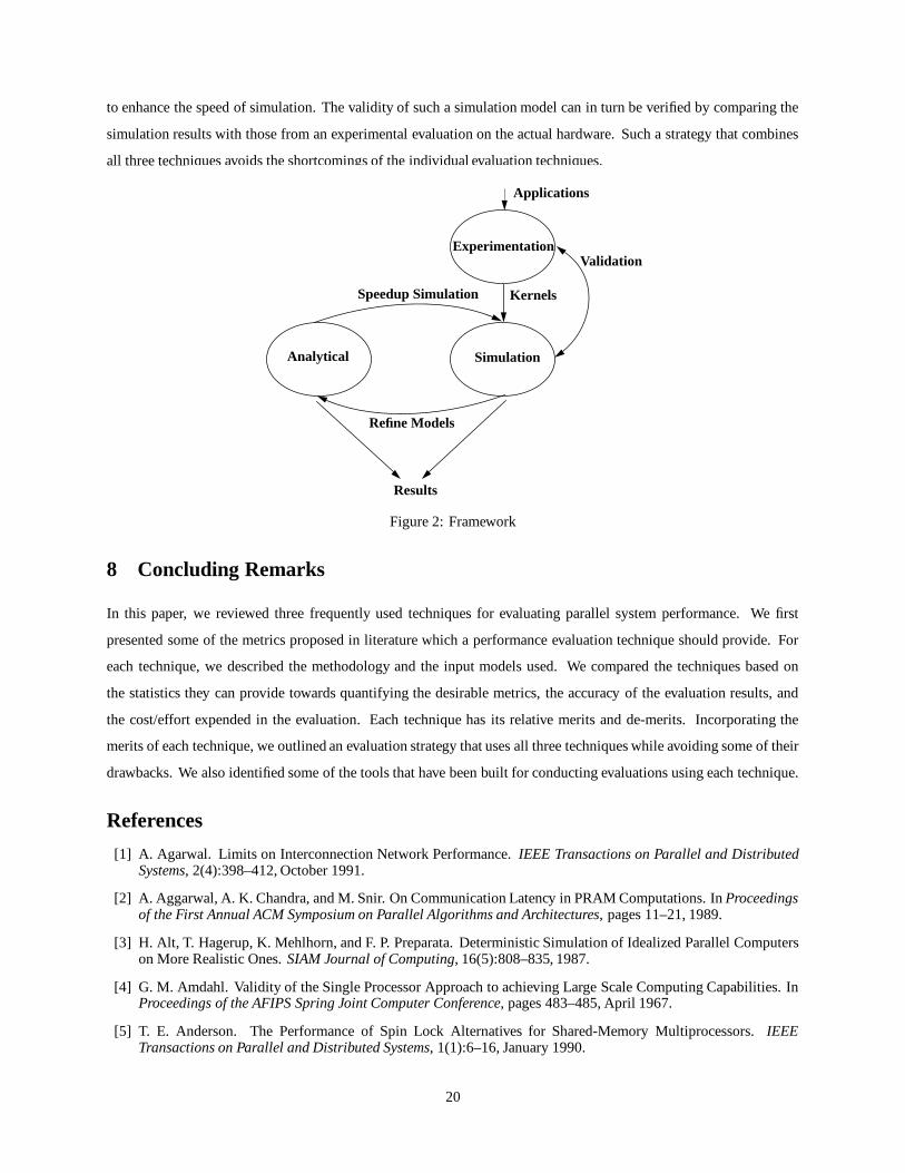
to enhance the speed of simulation. The validity of such a simulation model can in turn be verified by comparing the

simulation results with those from an experimental evaluation on the actual hardware. Such a strategy that combines

all three techniques avoids the shortcomings of the individual evaluation techniques.

Results

Analytical

Experimentation

Simulation

Kernels

Validation

Refine Models

Applications

Speedup Simulation

Figure 2: Framework

8 Concluding Remarks

In this paper, we reviewed three frequently used techniques for evaluating parallel system performance. We first

presented some of the metrics proposed in literature which a performance evaluation technique should provide. For

each technique, we described the methodology and the input models used. We compared the techniques based on

the statistics they can provide towards quantifying the desirable metrics, the accuracy of the evaluation results, and

the cost/effort expended in the evaluation. Each technique has its relative merits and de-merits. Incorporating the

merits of each technique, we outlined an evaluation strategy that uses all three techniques while avoiding some of their

drawbacks. We also identified some of the tools that have been built for conducting evaluations using each technique.

References

[1] A. Agarwal. Limits on Interconnection Network Performance. IEEE Transactions on Parallel and DistributedSystems, 2(4):398–412, October 1991.

[2] A. Aggarwal, A. K. Chandra, and M. Snir. On Communication Latency in PRAM Computations. In Proceedingsof the First Annual ACM Symposium on Parallel Algorithms and Architectures, pages 11–21, 1989.

[3] H. Alt, T. Hagerup, K. Mehlhorn, and F. P. Preparata. Deterministic Simulation of Idealized Parallel Computerson More Realistic Ones. SIAM Journal of Computing, 16(5):808–835, 1987.

[4] G. M. Amdahl. Validity of the Single Processor Approach to achieving Large Scale Computing Capabilities. InProceedings of the AFIPS Spring Joint Computer Conference, pages 483–485, April 1967.

[5] T. E. Anderson. The Performance of Spin Lock Alternatives for Shared-Memory Multiprocessors. IEEETransactions on Parallel and Distributed Systems, 1(1):6–16, January 1990.

20

[6] T. E. Anderson and E. D. Lazowska. Quartz: A Tool for Tuning Parallel Program Performance. In Proceedings ofthe ACM SIGMETRICS 1990 Conference on Measurement and Modeling of Computer Systems, pages 115–125,May 1990.

[7] J. Archibald and J-L. Baer. Cache Coherence Protocols : Evaluation Using a Multiprocessor Simulation Model.ACM Transactions on Computer Systems, 4(4):273–298, November 1986.

[8] D. Atapattu and D. Gannon. Building analytical models into an interactive performance prediction tool. InProceedings of Supercomputing ’89, pages 521–530, November 1989.

[9] D. Bailey et al. The NAS Parallel Benchmarks. InternationalJournal of Supercomputer Applications, 5(3):63–73,1991.

[10] M. Berry et al. The Perfect Club Benchmarks: Effective Performance Evaluation of Supercomputers. InternationalJournal of Supercomputer Applications, 3(3):5–40, 1989.

[11] E. L. Boyd, J-D. Wellman, S. G. Abraham, and E. S. Davidson. Evaluating the communication performance ofMPPs using synthetic sparse matrix multiplication workloads. In Proceedings of the ACM 1993 InternationalConference on Supercomputing, pages 240–250, July 1993.

[12] E. A. Brewer, C. N. Dellarocas, A. Colbrook, and W. E. Weihl. PROTEUS : A high-performance parallel-architecture simulator. Technical Report MIT-LCS-TR-516, Massachusetts Institute of Technology, Cambridge,MA 02139, September 1991.

[13] H. Burkhart and R. Millen. Performance measurement tools in a multiprocessor environment. IEEE Transactionson Computer Systems, 38(5):725–737, May 1989.

[14] R. Cole and O. Zajicek. The APRAM: Incorporating Asynchrony into the PRAM Model. In Proceedings of theFirst Annual ACM Symposium on Parallel Algorithms and Architectures, pages 169–178, 1989.

[15] R. G. Covington, S. Madala, V. Mehta, J. R. Jump, and J. B. Sinclair. The Rice parallel processing testbed. InProceedings of the ACM SIGMETRICS 1988 Conference on Measurement and Modeling of Computer Systems,pages 4–11, Santa Fe, NM, May 1988.

[16] M. E. Crovella and T. J. LeBlanc. Parallel Performance Prediction Using Lost Cycles Analysis. In Proceedingsof Supercomputing ’94, November 1994.

[17] D. Culler et al. LogP : Towards a realistic model of parallel computation. In Proceedings of the 4th ACMSIGPLAN Symposium on Principles and Practice of Parallel Programming, pages 1–12, May 1993.

[18] W. J. Dally. Performance analysis of k-ary n-cube interconnection networks. IEEE Transactions on ComputerSystems, 39(6):775–785, June 1990.

[19] H. Davis, S. R. Goldschmidt, and J. L. Hennessy. Multiprocessor Simulation and Tracing Using Tango. InProceedings of the 1991 International Conference on Parallel Processing, pages II 99–107, 1991.

[20] M. D. Dikaiakos, A. Rogers, and K. Steiglitz. FAST: A Functional Algorithm Simulation Testbed. In Proceedingsof MASCOTS ’94, pages 142–146, February 1994.

[21] J. Dongarra, O. Brewer, J. A. Kohl, and S. Fineberg. A tool to aid in the design, implementation, and understandingof matrix algorithms for parallel processors. Journal of Parallel and Distributed Computing, 9:185–202, 1990.

[22] T. H. Dunigan. Kendall Square Multiprocessor : Early Experiences and Performance. Technical ReportORNL/TM-12065, Oak Ridge National Laboratory, Oak Ridge, TN, March 1992.

[23] S. J. Eggers and R. H. Katz. The Effect of Sharing on the Cache and Bus Performance of Parallel Programs. InProceedings of the Third International Conference on Architectural Support for Programming Languages andOperating Systems, pages 257–270, Boston, Massachusetts, April 1989.

[24] S. J. Eggers, D. R. Keppel, E. J. Koldinger, and H. M. Levy. Techniques for efficient inline tracing on a sharedmemory multiprocessor. In Proceedings of the ACM SIGMETRICS 1990 Conference on Measurement andModeling of Computer Systems, pages 37–47, May 1990.

[25] T. Fahringer and H. P. Zima. A Static Parameter based Performance Prediction Tool for Parallel Programs. InProceedings of the ACM 1993 International Conference on Supercomputing, pages 207–217, July 1993.

21

[26] S. Fortune and J. Wyllie. Parallelism in random access machines. In Proceedings of the 10th Annual Symposiumon Theory of Computing, pages 114–118, 1978.

[27] P. B. Gibbons. A More Practical PRAM Model. In Proceedings of the First Annual ACM Symposium on ParallelAlgorithms and Architectures, pages 158–168, 1989.

[28] A. J. Goldberg and J. L. Hennessy. Mtool: An Integrated System for Performance Debugging Shared MemoryMultiprocessor Applications. IEEE Transactions on Parallel and Distributed Systems, 4:28–40, January 1993.

[29] S. R. Goldschmidt and J. L. Hennessy. The accuracy of trace-driven simulations of multiprocessors. In Proceedingsof the ACM SIGMETRICS 1993 Conference on Measurement and Modelingof Computer Systems, pages 146–157,May 1993.

[30] J. L. Gustafson, G. R. Montry, and R. E. Benner. Development of Parallel Methods for a 1024-node Hypercube.SIAM Journal on Scientific and Statistical Computing, 9(4):609–638, 1988.

[31] D. P. Helmbold and C. E. McDowell. Modeling Speedup (n) Greater than n. IEEE Transactions on Parallel andDistributed Systems, 1(2):250–256, April 1990.

[32] A. H. Karp and H. P. Flatt. Measuring Parallel processor Performance. Communications of the ACM, 33(5):539–543, May 1990.

[33] V. Kumar and A. Gupta. Analyzing Scalability of Parallel Algorithms and Architectures. In Proceedings of theACM 1991 International Conference on Supercomputing, Cologne, Germany, 1991.

[34] V. Kumar and V. N. Rao. Parallel Depth-First Search. International Journal of Parallel Programming, 16(6):501–519, 1987.

[35] J. Kuskin et al. The Stanford FLASH multiprocessor. In Proceedings of the 21th Annual InternationalSymposiumon Computer Architecture, pages 302–313, April 1994.

[36] D. Lenoski et al. The DASH Prototype: Logic Overhead and Performance. IEEE Transactions on Parallel andDistributed Systems, 4(1):41–61, January 1993.

[37] S. Madala and J. B. Sinclair. Performance of Synchronous Parallel Algorithms with Regular Structures. IEEETransactions on Parallel and Distributed Systems, 2(1):105–116, January 1991.

[38] M. Martonosi, A. Gupta, and T. Anderson. MemSpy: Analyzing Memory System Bottlenecks in Programs. InProceedings of the ACM SIGMETRICS 1992 Conference on Measurement and Modeling of Computer Systems,pages 1–12, June 1992.

[39] F. H. McMahon. The Livermore Fortran Kernels : A Computer Test of the Numerical Performance Range.Technical Report UCRL-53745, Lawrence Livermore National Laboratory, Livermore, CA, December 1986.

[40] P. Mehra, C. H. Schulbach, and J. C. Yan. A comparison of two model-based performance-prediction tech-niques for message-passing parallel programs. In Proceedings of the ACM SIGMETRICS 1994 Conference onMeasurement and Modeling of Computer Systems, pages 181–190, May 1994.

[41] J. M. Mellor-Crummey and M. L. Scott. Algorithms for Scalable Synchronization on Shared-Memory Multipro-cessors. ACM Transactions on Computer Systems, 9(1):21–65, February 1991.

[42] B. P. Miller et al. IPS-2: The Second Generation of a Parallel Program Measurement System. IEEE Transactionson Parallel and Distributed Systems, 1(2):206–217, April 1990.

[43] D. Nussbaum and A. Agarwal. Scalability of Parallel Machines. Communications of the ACM, 34(3):57–61,March 1991.

[44] S. Owicki and A. Agarwal. Evaluating the Performance of Software Cache Coherence. In Proceedings of theThird International Conference on Architectural Support for Programming Languages and Operating Systems,pages 230–242, Boston, Massachusetts, April 1989.

[45] J. H. Patel. Analysis of multiprocessors with private cache memories. IEEE Transactions on Computer Systems,31(4):296–304, April 1982.

22

[46] R. Ponnusamy, R. Thakur, A. Choudhary, K. Velamakanni, Z. Bozkus, and G. Fox. Experimental performanceevaluation of the CM-5. Journal of Parallel and Distributed Computing, 19:192–202, 1993.

[47] U. Ramachandran, G. Shah, S. Ravikumar, and J. Muthukumarasamy. Scalability study of the KSR-1. InProceedings of the 1993 International Conference on Parallel Processing, pages I–237–240, August 1993.

[48] S. K. Reinhardt et al. The Wisconsin Wind Tunnel : Virtual prototyping of parallel computers. In Proceedingsof the ACM SIGMETRICS 1993 Conference on Measurement and Modeling of Computer Systems, pages 48–60,Santa Clara, CA, May 1993.

[49] R. H. Saavedra, R. S. Gaines, and M. J. Carlton. Micro Benchmark Analysis of the KSR-1. In Proceedings ofSupercomputing ’93, pages 202–213, November 1993.

[50] S. K. Setia, M. S. Squillante, and S. K. Tripathi. Analysis of Processor Allocation in Multiprogrammed,Distributed-Memory Parallel Processing Systems. IEEE Transactions on Parallel and Distributed Systems,5(4):401–420, April 1994.

[51] J. B. Sinclair and W. P. Dawkins. ES: A Tool for Predicting the Performance of Parallel Systems. In Proceedingsof MASCOTS ’94, pages 164–168, February 1994.

[52] J. P. Singh, T. Joe, A. Gupta, and J. L. Hennessy. An Empirical Comparison of the Kendall Square ResearchKSR-1 and Stanford DASH Multiprocessors. In Proceedings of Supercomputing ’93, pages 214–225, November1993.

[53] J. P. Singh, E. Rothberg, and A. Gupta. Modeling communication in parallel algorithms: A fruitful interactionbetween theory and systems? In Proceedings of the Sixth Annual ACM Symposium on Parallel Algorithms andArchitectures, 1994.

[54] J. P. Singh, W-D. Weber, and A. Gupta. SPLASH: Stanford Parallel Applications for Shared-Memory. TechnicalReport CSL-TR-91-469, Computer Systems Laboratory, Stanford University, 1991.

[55] A. Sivasubramaniam, G. Shah, J. Lee, U. Ramachandran, and H. Venkateswaran. Experimental Evaluation ofAlgorithmic Performance on Two Shared Memory Multiprocessors. In Norihisa Suzuki, editor, Shared MemoryMultiprocessing, pages 81–107. MIT Press, 1992.

[56] A. Sivasubramaniam, A. Singla, U. Ramachandran, and H. Venkateswaran. An Approach to Scalability Study ofShared Memory Parallel Systems. In Proceedings of the ACM SIGMETRICS 1994 Conference on Measurementand Modeling of Computer Systems, pages 171–180, May 1994.

[57] A. Sivasubramaniam, A. Singla, U. Ramachandran, and H. Venkateswaran. A Simulation-based Scalability Studyof Parallel Systems. Journal of Parallel and Distributed Computing, 1994. To appear.

[58] X-H. Sun and J. L. Gustafson. Towards a better Parallel Performance Metric. Parallel Computing, 17:1093–1109,1991.

[59] L. G. Valiant. A Bridging Model for Parallel Computation. Communications of the ACM, 33(8):103–111, August1990.

[60] A. J. van Gemund. Performance Prediction of Parallel Processing Systems: The PAMELA Methodology. InProceedings of the ACM 1993 International Conference on Supercomputing, pages 318–327, July 1993.

[61] J. E. Veenstra and R. J. Fowler. MINT: A Front End for Efficient Simulation of Shared Memory Multiprocessors.In Proceedings of MASCOTS ’94, pages 201–207, February 1994.

[62] D. F. Vrsalovic, D. P. Siewiorek, Z. Z. Segall, and E. Gehringer. Performance Prediction and Calibration for aClass of Multiprocessors. IEEE Transactions on Computer Systems, 37(11):1353–1365, November 1988.

[63] H. Wabnig and G. Haring. PAPS - The Parallel Program Performance Prediction Toolset. In Proceedings of the7th International Conference on Modeling Techniques and Tools for Computer Performance Evaluation, Vienna,Austria, May 1994.

[64] P. J. Woest and J. R. Goodman. An Analysis of Synchronization Mechanisms in Shared Memory Multiprocessors.In Proceedings of the First International Symposium on Shared Memory Multiprocessing, pages 152–165, Tokyo,Japan, April 1991.

23

[65] J. Zahorjan and C. McCann. Processor Scheduling in Shared Memory Multiprocessors. In Proceedings of theACM SIGMETRICS 1990 Conference on Measurement and Modeling of Computer Systems, pages 214–225,1990.

24