a comparative phylogenetic approach to
TRANSCRIPT

1
A COMPARATIVE PHYLOGENETIC APPROACH
TO
AUSTRONESIAN CULTURAL EVOLUTION
Thesis submitted for the degree of
Doctor of Philosophy
to
Department of Anthropology
University College London
Fiona Marie Jordan
2007

2
ABSTRACT
Phylogenetic comparative methods were used to test hypotheses about cultural evolution
in ethnolinguistic groups from the Austronesian language family of the Pacific. The case
for quantitative statistical approaches to the empirical evolution of linguistic and cultural
features was presented. Phylogenetic trees of 67 Austronesian languages were constructed
using maximum parsimony and Bayesian Markov Chain Monte Carlo likelihood
algorithms on a database of lexical items.
The predominant transmission mode of 76 cultural traits was examined at the
macroevolutionary level with (i) partial Mantel matrix tests and (ii) multiple regression on
phylogenetic and geographic nearest neighbours. Mantel tests showed that both
geographic and phylogenetic transmission was correlated with cultural diversity.
Geographic distance had a greater overall partial correlation with cultural distance than
did phylogenetic distance, but only phylogenetic correlations were found with
kinship/social traits. Multiple regression on individual traits found that phylogenetic
nearest neighbours predicted more cultural traits, especially those involving the
inheritance of resources.
Ancestral states of kinship traits were reconstructed using a Bayesian comparative
method on a sample of 1000 phylogenies. The root of the tree was reconstructed as having
matrilocal post-marital residence and a bilateral, flexible descent system. Proto Oceanic
was reconstructed as unilocal and unilineal, and an hypothesis of matriliny and
matrilocality could not be rejected. Murdock’s main-sequence theory of the co-evolution of
post-marital residence and descent systems was tested. The most likely model of the
evolutionary pathway demonstrated that residence changed before descent. Rates of
change in residence and descent traits were estimated. A co-evolutionary hypothesis of
matriliny and male absence was tested. Contrary to anthropological theory, a high
3
dependence on fishing showed no clear pattern of co-evolution with matrilineal social
organisation.
Population size of the language community was hypothesized to be a factor
influencing lexical change. Conventional statistics showed a significant strong inverse
correlation, indicating a relationship between small populations and accelerated lexical
change. This correlation disappeared when comparative methods were used to control for
phylogeny. Population size appeared to be evolving according to a drift model, while
lexical change did not fit a neutral model of evolution.

4
TABLE OF CONTENTS
Page
Abstract 2
Table of Contents 4
List of Tables 14
List of Figures 16
List of Abbreviations 19
Acknowledgements 20
Frontpiece 21
Chapter 1. The phylogenetic approach to cultural evolution 22
1.1 Summary 22
1.2 Culture and evolution: History and current approaches 23
1.2.1 History 23
1.2.1.1 Cultural ecology 24
1.2.1.2 Sociobiology 24
1.2.2 Current approaches 25
1.2.2.1 Evolutionary psychology 25
1.2.2.2 Human behavioural ecology 25
1.2.2.3 Dual-inheritance theories 26
1.2.2.4 Population history 27
1.2.3 Cultural phylogenetics 28
1.3 Culture has Darwinian properties 29
1.3.1 Similarities between biological and cultural evolution 31
1.3.1.1 Language evolution 31
1.3.2 Differences between biological and cultural evolution 34
1.3.2.1 Many cultural parents 34
1.3.2.2 Cultural evolution can be rapid 35
1.3.2.3 Multiple lineages and multiple phenotypes 35
1.3.3 Units of culture 36
1.3.3.1 Core and periphery 36
1.3.3.2 Culture as species 37
1.3.3.3 Horizontal transmission 38

5
Page
1.4 The phylogenetic approach to cultural evolution 39
1.4.1 Summary 39
1.4.2 Cross-cultural comparison and Galton’s Problem 39
1.4.3 Methods to address Galton’s Problem 43
1.4.3.1 Sampling methods 43
1.4.3.2 Controlled comparison 44
1.4.3.3 Autocorrelation 44
1.4.3.4 Phylogenetically controlled comparison 44
1.4.4 Language phylogenies 45
1.4.5 Material culture phylogenies 47
1.4.6 Comparative tests of cultural hypotheses 48
1.4.6.1 Matriliny and cattle in the Bantu 49
1.4.6.2 Worldwide sex ratio and marriage costs 50
1.4.6.3 Marriage transfers in Indo-European societies 51
1.4.7 Objections to phylogenetic and comparative methods 51
1.4.8 Simulations 54
1.4.9 Different lines of evidence 56
1.5 The ethnographic context: Austronesian cultures of the Pacific 57
1.5.1 Summary 57
1.5.2 Pacific colonisation 58
1.5.3 Austronesian languages 62
1.5.3.1 Austronesian subgrouping 62
1.5.4 The Austronesian dispersal 64
1.5.5 Models of colonisation 66
1.5.5.1 Express train / Out of Asia 66
1.5.5.2 Entangled bank 66
1.5.6 Molecular anthropology in the Pacific 67
1.5.6.1 Mitochondrial DNA 67
1.5.6.2 Y-chromosome lineages 68
1.5.6.3 Autosomal markers 68
1.5.6.4 Sex-specific patterns of dispersal 69
1.5.7 An integrated model 70
1.5.8 Later developments in Austronesian history 70
1.6 Cultural evolution in the Pacific 71

6
Page
1.6.1 Islands as laboratories 71
1.6.2 Evolutionary approaches 72
1.7 Austronesian kinship 74
1.7.1 Descent 74
1.7.2 Residence 75
1.7.2.1 Parental investment 75
1.7.3 Previous work 75
1.8 Structure of the thesis 76
Chapter 2. Phylogenetic methods & Austronesian language trees 80
2.1 Summary 80
2.2 Introduction 81
2.2.1 Phylogenetic methods 81
2.2.2 Phylogenetic trees of human populations 81
2.2.3 Language phylogenies 82
2.2.4 Historical linguistics 83
2.2.5 Computational methods for language phylogenies 84
2.2.6 Survey of studies 85
2.2.7 Algorithms for inferring evolutionary trees 87
2.2.8 Non-tree methods 89
2.3 Bayesian methods 89
2.3.1 Bayesian inference of phylogeny 89
2.3.2 Markov chain Monte Carlo 91
2.3.3 Support for nodes: Posterior probability distributions 91
2.4 Phylogenetic trees of Austronesian languages 92
2.4.1 Aims 92
2.4.2 Austronesian Comparative Dictionary 92
2.4.3 Austronesian Basic Vocabulary Database 93
2.4.4 Data used in this thesis 95
2.5 Tree searches using parsimony 95
2.5.1 Tree searches using parsimony: The 80 language data set 95
2.5.1.1 Bootstrap analysis 96
2.5.2 Results 96
2.5.3 Tree topology 98

7
Page
2.6 Tree searches using Bayesian methods 99
2.6.1 Bayesian estimation of phylogeny 99
2.6.2 Analyses 100
2.6.2.1 Initial Bayesian analyses 100
2.6.2.2 Models of word evolution and the choice of priors 100
2.6.2.3 Outgroup rooting 101
2.6.3 Results 102
2.6.3.1 MCMC sample 102
2.6.3.2 Autocorrelation 102
2.6.4 Bayesian phylogeny 105
2.6.5 Topology 109
2.6.6 Comparison with other results 111
2.7 Conclusions 112
Chapter 3. The comparative method in anthropology 113
3.1 Summary 113
3.2 Introduction 114
3.2.1 The comparative method 114
3.3 Parsimony-based 115
3.3.1 Characteristics of parsimony-based comparative methods 115
3.3.1.1 Shortcomings of parsimony 116
3.4 Likelihood comparative methods 118
3.4.1 Characteristics of likelihood-based comparative methods 118
3.4.1.1 Pagel’s method 118
3.4.2 Bayesian comparative methods 120
3.4.2.1 BayesMultiState 121
3.4.3 Model testing using reversible-jump MCMC 122
3.4.3.1 Reverse-jump MCMC 123
3.4.3.2 Bayes factor 123
3.5 Conclusions 124

8
Chapter 4. Do cultures resemble their neighbours or their cousins?
A test of phylogenetic and geographic distance 125
4.1 Summary 125
4.2 Introduction 126
4.2.1 Cultural transmission between groups 126
4.2.2 Macroevolutionary studies of between-group cultural transmissions 127
4.2.3 Adaption and ecology 130
4.2.4 Cultural transmission in Austronesian societies 131
4.2.4.1 Replication 131
4.2.4.2 Alternative approaches 132
4.3 Mantel tests of cultural, geographic, and linguistic distances 133
4.3.1 Aim 133
4.3.2 Distance matrices for tests of diversity 133
4.3.3 Hypotheses 134
4.3.4 Data 135
4.3.4.1 Cultural data 135
4.3.4.2 Language data 135
4.3.4.3 Geographic data 136
4.3.5 Mantel matrix tests 138
4.3.5.1 Program 139
4.3.6 Distance matrices 139
4.3.6.1 Cultural distances 139
4.3.6.2 Linguistic distances 139
4.3.6.3 Geographic distances 140
4.3.6.4 Population size 140
4.3.7 Matrix correlations 141
4.3.7.1 Geographic distance 141
4.3.7.2 Population size 141
4.3.7.3 Cultural distance 141
4.3.7.4 Language and geography 143
4.3.8 Mantel tests: Discussion 143
4.3.8.1 Alternative models 144
4.4 Nearest neighbour analysis 145
4.4.1 Aim 145
4.4.2 Phylogenetic and geographic nearest neighbours 145
9
Page
4.4.3 Estimating nearest neighbours 145
4.4.4 Logistic regression analysis 147
4.4.5 Results of nearest neighbour tests 148
4.4.6 Nearest neighbour tests: Discussion 154
4.5 Cultural transmission: Discussion 155
4.5.1 Comparison with previous work 155
4.5.2 Consideration of the methodologies 157
4.5.3 Conclusion 158
Chapter 5. Ancestral states of descent and residence 160
5.1 Summary 160
5.2 Introduction 161
5.2.1 Descent 161
5.2.2 Residence 165
5.2.3 Austronesian descent and residence 165
5.3 Ancestral states 169
5.3.1 Debates in the literature: Bilateral or lineal? 170
5.3.2 Were early Austronesian societies matrilineal? 172
5.3.3 Evolutionary interpretations of kinship structure 173
5.3.4 Inferring ancestral states 174
5.3.5 Questions 175
5.4 Methods 176
5.4.1 Linguistic data 176
5.4.2 Cultural data 176
5.4.2.1 Coding: Descent 188
5.4.2.2 Coding: Post-marital residence 189
5.4.3 Phylogeny estimation 196
5.4.4 Estimation of ancestral states 196
5.5 Results 198
5.5.1 Phylogeny 198
5.5.2 Ancestral state reconstructions 198
5.5.3 Descent: Multi-state coding 200
5.5.3.1 Ancestral states 200
5.5.3.2 Rates of trait switching 203

10
Page
5.5.4 Inheritance: Multi-state coding 203
5.5.4.1 Ancestral states 203
5.5.4.2 Rates of trait switching 204
5.5.5 Descent: Lineality 207
5.5.5.1 Ancestral states 207
5.5.5.2 Rates of trait switching 210
5.5.6 Descent: Matrilineal aspect 210
5.5.6.1 Ancestral states 210
5.5.6.2 Rates of trait switching 213
5.5.7 Residence: Scale 213
5.5.7.1 Ancestral states 213
5.5.8 Residence: Primary mode 214
5.5.8.1 Ancestral states 214
5.5.8.2 Rates of trait switching 217
5.5.9 Residence: Matrilocal aspect 217
5.5.9.1 Ancestral states 217
5.5.9.2 Rates of trait switching 218
5.5.10 Residence: Flexibility 221
5.5.10.1 Ancestral states 221
5.5.10.2 Rates of trait switching 221
5.5.11 Summary of ancestral states results 225
5.5.12 Was Proto Oceanic matrilineal and/or matrilocal 225
5.5.13 Contribution of phylogenetic uncertainty 226
5.6 Discussion 227
5.6.1 Austronesian matriliny 228
5.6.2 Flexible kinship systems 229
5.6.3 Comparative methodologies 230
5.7 Conclusion 231
Chapter 6. Cause and effect in social organisation:
Correlated evolution of descent and residence 232
6.1 Summary 232
6.2 Introduction 233
6.2.1 Questions 234

11
Page
6.3 Testing the “main sequence” 235
6.3.1 Introduction 235
6.3.1.1 Hypotheses 237
6.3.2 Methods 238
6.3.2.2 Cultural data and coding schemes 238
6.3.2.3 Testing correlated evolution 239
6.3.2.4 Using RJ MCMC to find the best models of evolutionary
change
241
6.3.2.5 Hypothesis testing 243
6.3.2.6 Using kappa to estimate the mode of character evolution 243
6.3.3 Results 244
6.3.3.1 Phylogeny 244
6.3.3.2 Chi-square tests 244
6.3.3.3 Kappa 244
6.3.3.4 Tests for co-evolution 247
6.3.3.5 Rates of change over time 255
6.3.4 Discussion 258
6.3.4.1 Scenarios for the evolution of Austronesian unilocal and
unilineal forms
258
6.3.4.2 Patrilineal organisation in Austronesian societies 260
6.3.4.3 Rates of cultural evolution 262
6.3.4.4 Desirability of multi-state models 262
6.4 Is matriliny co-evolving with male absence? 264
6.4.1 Introduction 264
6.4.1.1 Hypotheses 267
6.4.2 Methods 267
6.4.2.1 Phylogeny estimation 267
6.4.2.2 Cultural data and coding schemes 267
6.4.2.3 Testing for correlated evolution 274
6.4.3 Results 274
6.4.3.1 Phylogenetic analysis 274
6.4.3.2 Kappa and chi-square tests 275
6.4.3.3 Tests for correlated evolution 277
6.4.3.4 Identifying models of evolutionary change 277

12
Page
6.4.3.5 Results of an earlier analysis 281
6.4.4 Discussion 282
6.4.4.1 Alternative explanations for matriliny 285
6.4.4.2 Does isolation break down matriliny? 287
6.5 Conclusion 288
Chapter 7. Evolutionary analyses of lexical change and
population size 290
7.1 Summary 290
7.2 Introduction 291
7.2.1 Language change 291
7.2.2 Founder effects 292
7.2.3 Punctuated equilibrium 293
7.2.4 Demography and the rate of change in biosocial variables 293
7.2.5 Modelling the rate of word evolution 294
7.2.6 Models of neutral or random change 296
7.2.7 Aims of the study 297
7.3 Data 298
7.3.1 Demographic data 298
7.3.2 Language data 299
7.3.3 Geographic data 299
7.4 Analysis and results 299
7.4.1 Phylogenetic trees 299
7.4.2 Calculating language change 301
7.4.3 Statistical tests 304
7.4.3.1 Language-specific change 308
7.4.4 Phylogenetically controlled analyses 309
7.4.5 Drift versus directional models of evolution 310
7.4.6 Mode and tempo of evolution 311
7.4.7 Phylogenetic tests of correlated evolution 313
7.4.8 The power law: A null model of change 314
7.5 Discussion 316
7.5.1 Findings of the present study 316
7.5.2 Power law distributions 318
13
Page
7.5.3 Alternative explanations 319
7.5.3.1 Selection 319
7.5.3.2 Contact 319
7.5.3.3 Ecology 320
7.5.4 Limitations 321
7.5.5 Conclusions 322
Chapter 8. Concluding remarks 323
8.1 Is a “comparative phylogenetic approach” necessary? 323
8.2 Are we “butterfly-collecting”? 325
8.3 Should we use language trees? 326
8.4 Are simple models justified? 328
8.5 The central role of kinship 329
8.6 Cultural evolution in the Austronesian world 330
References 333
Appendix A: Data on the Austronesian societies and their
corresponding languages
368
Appendix B: Ethnographic Atlas (Murdock 1967) variables recoded
into dichotomous categories
373

14
LIST OF TABLES
Table Page
1.1 Parallels between biological and culture systems 32
1.2 Variation in Austronesian descent systems 74
2.1 Survey of published linguistic phylogenies 86
3.1 Comparison of parsimony and likelihood-based comparative methods 117
4.1 Correlations between geographic, linguistic, and cultural distance matrices 142
4.2 Summary results of nearest neighbour analysis 148
4.3 Binary logistic regression on geographic and phylogenetic nearest
neighbours
149
5.1 Frequency of descent and residence types 168
5.2 Information on descent for 67 Austronesian societies 177
5.3 Information on inheritance for 67 Austronesian cultures 182
5.4 Information on post-marital residence for 67 Austronesian societies 191
5.5 Summary table of ancestral state reconstructions at four deep nodes 224
5.6 Fossilisation analyses 226
5.7 Estimates of the between- and within-tree components of variance 227
6.1 Contingency tables for unilineal/unilocal systems 239
6.2 Description of the rate coefficients as applied to residence/descent data 248
6.3 Unilineal/unilocal data: most frequent models found by RJ MCMC model-
search
253
6.4 Patrilineal/patrilocal data: most frequent models found by RJ MCMC
model-search
253
6.5 Probability of change in descent and residence over three time periods 256
6.6 Contingency tables for matriliny and fishing 268
6.7 Information on fishing for 67 Austronesian societies 269
15
Table Page
6.8 Description of the rate coefficients as applied to matri-traits and fishing 275
6.9 Matriliny and fishing data: most frequent models found by RJ MCMC
model-search
281
7.1 Population data, total lexical change, and terminal branch length 302
7.2 Correlations of language population size and amount of lexical replacement 307
7.3 Correlations of terminal branch lengths 308
7.4 Maximum-likelihood estimates of three scaling parameters 312
16
LIST OF FIGURES
Figure Page
1.1 A demonstration of Galton’s Problem 41
1.2 Tree terminology 42
1.3 Map of the Pacific showing geographic and culture areas 60
1.4 Map of the Pacific showing the extent of the Austronesian language
family
61
1.5 Subgrouping of the Austronesian language family 63
2.1 Basic principles of computational linguistic phylogenetics 88
2.2 Shortest tree of 77 Austronesian languages found by parsimony
analysis
94
2.3 Maximum parsimony tree of 80 Austronesian languages 97
2.4 Convergence of the Markov chain 103
2.5 Posterior probability distribution of log-likelihoods 104
2.6 Consensus linguistic tree of the 1000-tree Bayesian sample 106
2.7 Six random trees from the Bayesian sample 108
3.1 The two models estimated in Pagel’s likelihood/Bayesian methods 119
4.1 Why do populations share cultural traits? 128
4.2 Geographical location of the 80 Austronesian societies 137
4.3 Estimation of phylogenetic nearest neighbours 146
5.1 Traditional kinship diagrams 164
5.2 Geographical distribution and form of descent in 67 Austronesian
cultures
166
5.3 Geographical distribution and form of residence in 67 Austronesian
cultures
167
5.4 Consensus phylogeny of 1000 Bayesian trees for 67 Austronesian
languages
199
17
5.5 Ancestral state reconstruction of descent 201
5.6 Posterior probability distribution of descent with multi-state
characters
202
Figure Page
5.7 Ancestral state reconstruction of inheritance 205
5.8 Posterior probability distribution of inheritance 206
5.9 Ancestral state reconstruction of bilateral versus lineal descent 208
5.10 PPD of bilateral versus lineal descent 209
5.11 Ancestral state reconstruction of a matrilineal aspect in descent 211
5.12 PPD of a matrilineal aspect of descent 212
5.13 Ancestral state reconstruction of the primary mode of residence 214
5.14 PPD of residence with multi-state characters 216
5.15 Ancestral state reconstruction of a matrilocal residence 219
5.16 PPD of residence with a matrilocal option 220
5.17 Ancestral state reconstruction of flexible systems of residence 222
5.18 PPD of flexibility in residence 223
6.1 The dependent model of evolution 240
6.2 Consensus phylogeny of 67 Austronesian societies’ phylogeny
showing the evolution of unilineal descent and unilocal residence
245
6.3 Phylogeny showing the evolution of patrilineal descent and patrilocal
residence
246
6.4 Distribution of estimated kappa values for patri-coding 247
6.5 Evolutionary flow diagram for descent and residence (unilineal
coding)
249
6.6 Evolutionary flow diagram of descent and residence (patri-coding) 250
6.7 Log-likelihoods of the independent and dependent model 251
6.8 Posterior distributions of the rate coefficients for unilineal descent
and unilocal residence
252
18
6.9 Probability of change over time in each of eight transitions 257
6.10 Phylogeny showing the evolution of matrilineal descent and high
dependence on male fishing
276
6.11 “Flow diagram” for matriliny and fishing 278
6.12 Posterior distribution panels for matriliny and fishing 279
Figure Page
7.1 Phylogeny of a 500-tree Bayesian sample showing population size 300
7.2 Total lexical change for two languages 301
7.3 Scatterplot showing the relationship between total lexical change and
language population size
305
7.4 Distributions of (i) permuted data and (ii) obtained correlations 306
7.5 Log-log scatterplots of lexical change and population size versus their
ranks
315

19
LIST OF ABBREVIATIONS
ABV Austronesian Basic Vocabulary
ACD Austronesian Comparative Dictionary
AN Austronesian
BP years before the present
CMP Central Malayo-Polynesian
EA Ethnographic Atlas
EMP Eastern Malayo-Polynesian
HRAF Human Relations Area Files
MCMC Markov-chain Monte Carlo
ML maximum likelihood
MP Malayo-Polynesian
MP maximum parsimony
OC Oceanic
PCE Proto Central-Eastern
PPD posterior probability distribution
SCCS Standard Cross-Cultural Sample
SH–WNG South Halmahera—West New Guinea
SIL Summer Institute of Linguistics
WMP Western Malayo-Polynesian
Note: The addition of “P” before language subgroups denotes “Proto” (e.g. POC = Proto Oceanic).
20
ACKNOWLEDGEMENTS
This work is in large part concerned with cultural transmission and kinship networks, and
here I would like to acknowledge both in the completion of my thesis. Warm thanks above
all to my supervisor, Ruth Mace, who has always made the hard tasks seem possible. I
greatly appreciate her stimulating intellectual “vertical transmission”, but also her
constant support, especially by negotiating a way for me to return to the PhD at a time
when it seemed quite impossible. Thank you, Ruth, for the high-quality investment.
Without the superb efforts of Russell Gray, Simon Greenhill, and Robert Blust on
the Austronesian Basic Vocabulary database, and their gracious generosity in granting me
access to the language data, my research could not have progressed. Russell also provided
encouragement and advice, and Simon took time to give me valuable and amusing
comments on work in progress.
The vastly clever Mark Pagel and Andrew Meade designed the Bayesian software
used in the thesis. They gave up generous amounts of time to teach me arcane lore about
Unix and probabilities, and were on call to help run analyses and fix glitches. I am
extremely grateful for their help. Many thanks also to my colleagues in the CECD, “Culture
Club”, and the Department of Anthropology, especially Stephen Shennan and Gillian
Bentley for academic guidance, and Tom Currie, Laura Fortunato, and Mhairi Gibson for
friendship and unflagging encouragement. Especial thanks to Tom for his GIS skills and
help with mapping.
To my friends and family who have been such great cheerleaders in the face of an
incomprehensible project, thank you so much. To Rachel, thank you for making me
smile—about everything.
This work was funded by the Association of Commonwealth Universities.

21
The thousands of societies that exist today, or once existed on the surface of the earth,
constitute so many experiments, the only ones we can make use of to formulate and test
our hypotheses, since we can’t very well construct them or repeat them in the laboratory …
These experiments, represented by societies unlike our own, described and analyzed by
anthropologists, provide one of the surest ways to understand what happens in the human
mind and how it operates. That’s what anthropology is good for in the most general way
and what we can expect from it in the long run.
(Levi-Strauss 1972:41)
Why, for example, is it a nonpossibility for a terminological system to recognize not two,
but three or four sexes; for new marriages to take place after each pregnancy, the first
monogamous, the second polyandrous, the third polygynous; or why not descent which is
patrilineal in the morning, matrilineal in the afternoon, bilateral in the evening, and
double on Sundays? Shall we not ask, in other words, why elephants do not have two
heads, why cabbages do not grow on clouds, and why the moon is not made of Swiss
cheese? The limited possibilities of nature are none other than the forms which evolution
has produced. The task of science is to explain why they were produced.
(Harris 2001:626)

22
CHAPTER ONE
THE PHYLOGENETIC APPROACH TO CULTURAL EVOLUTION
1.1 Summary
The last 25 years have seen the establishment of a strong Darwinian programme with
multiple subfields in the social sciences (Barkow, Cosmides, and Tooby 1992; Cronk,
Chagnon, and Irons 2000; Barrett, Dunbar, and Lycett 2001). Within this programme
is the emerging field of cultural evolution (Cavalli-Sforza and Feldman 1981; Boyd and
Richerson 1985, 1996; Durham 1991, 1992; Mesoudi, Whiten, and Laland 2004;
Richerson and Boyd 2005), which may be broadly defined as the application of models
and methods from evolutionary biology to investigate cultural processes and patterns.
The scope of this endeavour includes among other questions, the study of (i) diversity:
the patterns of culture traits in space and time; (ii) change: cultural transmission and
innovation; and (iii) adaptation: which aspects of culture co-evolve? Evolutionary
biologists adopt a phylogenetic approach to these questions, that is, they take historical
relationships between species into account by using evolutionary tree diagrams
(Harvey and Pagel 1991). Anthropologists are now beginning to study cultural
evolution, and the questions above, with a similar set of tools (e.g. Holden and Mace
1997, 1999; Sellen and Mace 1997, 1999; Mace and Holden 1999, 2004; Collard and
Shennan 2000; Gray and Jordan 2000; Borgerhoff Mulder 2001; Borgerhoff Mulder,
George-Cramer, Eshleman, and Ortolani 2001; O’Brien, Darwent, and Lyman 2001;
Holden 2002; Shennan 2002; Tehrani and Collard 2002; Gray and Atkinson 2003;
Jordan and Shennan 2003; Mace, Jordan, and Holden 2003; Fortunato, Holden, and
Mace 2006; also see volumes edited by Lipo, O’Brien, Shennan, and Collard 2005;
Mace, Holden, and Shennan 2005; Forster and Renfrew 2006).
23
In this chapter, I briefly review the history of cultural evolutionary studies,
including the relevant current approaches. I then outline the analogy between
biological and cultural systems, and address the implications of differences between
these evolutionary systems. “Galton’s Problem”—the non-independence of cultures—is
introduced as a prelude to the phylogenetic approach. I review current work in
“cultural phylogenetics” that has used both tree-building methods and comparative
(co-evolutionary) tests on linguistic, cultural, and archaeological data. Finally, I
introduce the ethnographic context of this thesis, the Austronesian-speaking societies
of the Pacific, and outline the hypotheses to be tested in the subsequent chapters.
1.2 Culture and evolution: History and current approaches
1.2.1 History
In The Descent of Man, Darwin recognised that the evolutionary processes he
described could be seen in aspects of human culture as well as in the biological world.
Of language, he noted “striking homologies due to community of descent” (1871:60).
However, anthropological applications of Darwin’s theories by the early “cultural
evolutionists” in the 19th century (Tylor 1871 [1973]; Morgan 1877 [1964]) took a naïve
unilinear view of evolution, positing that cultures could be placed along scales of
progress or development towards some “civilised” ideal. Discredited as racist, these
ideas were roundly rejected by relativist social anthropologists such as Boas (1948) and
Malinowski (1944 [1970]), who sought to contextualise cultures on their own terms.
Beginning in the early 20th century, the large-scale collection of ethnographic
information by field anthropologists allowed researchers to test hypotheses about
cultural diversity by the method of cross-cultural comparison. The Human Relations
Area Files (HRAF) (Murdock 1954), Standard Cross-Cultural Sample (SCCS)
(Murdock and White 1969), and Murdock’s (1967) Ethnographic Atlas (EA) all acted
as systematic repositories of comparative cultural information, useful for testing
24
correlations in cultural traits. Researchers have used these resources to uncover
worldwide correlates in cultural traits such as polygyny (Whiting 1964; White and
Burton 1988), warfare (Otterbein and Otterbein 1965) and inheritance (Murdock
1949). While sometimes using evolutionary terminology, these cross-cultural analyses
did not however comprise a formal approach to cultural evolution.
1.2.1.1 Cultural ecology
Mid-20th century, cultural ecologists used evolutionary concepts such as adaptation
and radiation to examine and interpret human-environment interactions (White 1949;
Steward 1955; Sahlins and Service 1960; Vayda 1969). In particular, these workers
were interested to what degree local environments constrained and influenced core
aspects of culture, and whether in this respect human societies followed any general
rules. Investigations of this type, however, did not occur within an explicitly Darwinian
framework.
1.2.1.2 Sociobiology
The emergence of behavioural ecology and sociobiology in the 1970s (Wilson 1975;
Dawkins 1976; Krebs and Davies 1997) led some workers to examine culture through a
new kind of evolutionary lens, using the theoretical and methodological tools of
evolutionary biology and behavioural ecology (Alexander 1979; Chagnon and Irons
1979; Lumsden and Wilson 1981). The fragmentation of the sociobiological movement
(Segerstrale 2001) resulted in a number of current subfields that derive from this
evolutionary-informed perspective. While sharing a central Darwinian worldview
about human behaviour, there are three broad schools of thought that differ in their
methodologies, the kinds of questions they ask, and their approaches to concepts such
as fitness and adaptation (Laland and Brown 2002). These three are discussed below,
along with approaches to population history, as an introduction to cultural
phylogenetics.
25
1.2.2 Current approaches
1.2.2.1 Evolutionary psychology
Evolutionary psychology (Barkow et al. 1992), one of these three subfields, aims to
identify the selection pressures in the past that shaped the design of our cognitive
mechanisms. On this view, these psychological mechanisms respond to environmental
input to produce our behaviours, including “evoked” cultural behaviours (Tooby and
Cosmides 1989). Evolutionary psychologists are more interested in behaviour thought
to be universally human rather than in explaining cultural diversity, for example,
cross-cultural patterns in mate-choice (Buss 1989) or mechanisms for the detection of
cheaters in social contracts (Cosmides and Tooby 1989). For evolutionary
psychologists, it is the brain architecture producing cultural traits that evolves, and
thus the selection pressures on that brain organisation that are of interest.
1.2.2.2 Human behavioural ecology
A second subfield has its roots in animal behaviour. The central tenet of behavioural
ecology is that organisms act in ways that maximise their reproductive success; the
field examines individual behaviour in the context of fitness-maximisation or
optimality models (Krebs and Davies 1997). In human behavioural ecology (HBE),
adaptive hypotheses are tested in specific ecological contexts, under the assumption
that humans flexibly alter their behaviour to meet Darwinian goals in a changing
environment (Mace 2000). For example, where men control wealth, the polygyny
threshold model predicts that women will choose to enter a polygynous marriage if this
will provide more resources than a monogamous union (Borgerhoff Mulder 1990). The
HBE field uses empirical data to test hypotheses about cultural diversity (e.g. Smith
and Winterhalder 1992; Cronk et al. 2000), and with this perspective, cultural
behaviour—the capacity for which is itself an evolved adaptation—is viewed as another
adaptive phenotypic response to, or part of, the environment. Cultural behaviours that
promote individual reproductive success are assumed more adaptive, and hence more

26
likely to be adopted or maintained. The spread of some cultural traits, however, cannot
be explained in terms of differential reproductive success, as changes take place in less
than a generation. Therefore, supplementary models are needed (Boone and Smith
1998).
1.2.2.3 Dual-inheritance theories
A third current evolutionary approach to culture is frequently mathematical in focus
and is variously termed gene-culture co-evolutionary theory, evolutionary culture
theory or dual-inheritance theory (Richerson and Boyd 1978; Durham 1990; Laland
and Brown 2002). The dynamics of cultural transmission are modeled using the
techniques of population genetics, exploring how cultural traits can not only co-evolve
with and influence biological evolution, but how they can evolve independently via a
separate inheritance system (Cavalli-Sforza and Feldman 1981; Boyd and Richerson
1985, 1992; Durham 1991; Laland, Kumm, and Feldman 1995; Boyd et al. 1997;
Richerson and Boyd 2005). Social learning from conspecifics alters the dynamics of
behaviour in a group, as each individual does not have to learn through individual
trial-and-error.
Dual inheritance models stress the importance of social learning opportunities
as a factor in the transmission of cultural traits and demonstrate how cultural change
can arise because of transmission biases (Boyd and Richerson 1985, 2005). Direct bias,
where a trait is chosen because of some intrinsic property of its own, is a form of
cultural selection. Indirect bias is found where traits are chosen due to some aspect of
the model and includes biases such as conformist transmission, where traits are more
likely to be adopted because they are common or the norm, and prestige bias, where
the association of a trait with a prestigious individual makes it more likely to be
adopted (Henrich and Gil-White 2001). These social learning dynamics can also be
useful in exploring how so-called maladaptive cultural traits may evolve, such as
smoking (Feldman and Laland 1996), and how adaptive traits may be lost, as with the

27
pre-contact Tasmanian toolkit that Henrich (2004) suggests was caused by
depopulation, thus leading to a critical lack of expert teachers.
1.2.2.4 Population history
Gene-culture co-evolution examines how individual cultural traits could be co-
evolving together with aspects of human biology. For example, in the Kwa-speaking
populations in West Africa, sickle-cell anaemia appears to be an adaptive response to
the malarial conditions created by slash-and-burn agriculture (Durham 1991).
Similarly, the evolution of lactose tolerance genes in some populations appears to be
associated with cattle farming and milk-drinking (Feldman and Cavalli-Sforza 1989;
Durham 1991; Mace and Holden 1997). Other approaches to cultural evolution have
looked at the degree to which genes and culture evolve together through space and
time; that is, if ethnolinguistic groups are enduring entities with a population history.
Cavalli-Sforza and colleagues (Cavalli-Sforza, Piazza, Menozzi, and Mountain 1988;
Cavalli-Sforza, Minch, and Mountain 1992; Cavalli-Sforza, Menozzi, and Piazza 1994)
made an attempt to demonstrate a high correspondence, indicative of parallel
dispersal/migration processes, between worldwide linguistic and genetic groups.
Genes and languages are both attributes of human populations, so when a population
splits, then the linguistic and genetic characteristics of the groups will also tend to
show divergence over time. At the broad scale, their results appeared generally robust
given that the strength of correlations will depend on how information is transmitted;
to the extent that languages transmit horizontally, we should expect imperfect
correlations (Penny, Watson, and Steel 1993).
Other researchers (Chen, Sokal, and Ruhlen 1995) and those working at finer
regional scales (e.g. Lum 1998 for Oceania) have also claimed consistent
correspondences between phylogenies derived from genetic and language data.
However, there can be high levels of exchange between humans groups (Bateman et al.
1990; Moore 1994) and we find evidence that genes and culture do not always evolve
together; for example, Lapp populations in Finland genetically resemble other Indo-

28
European populations, but speak an unrelated Uralic language (Cavalli-Sforza et al.
1994).
These studies embody the issues of a larger debate concerning to what degree
genes, languages, and culture are related in human prehistory (Renfrew 1987;
Bateman et al. 1990; Moore 1994, 2001; Dewar 1995; Bellwood 1996b; Kirch and
Green 1997; Sims-Williams 1998; Terrell, Hunt, and Gosden 1997; Terrell, Kelly, and
Rainbird 2001). Phylogenetic processes, emphasising the dispersal and migration of
groups, and reticulate or “rhizotic” processes, emphasising network-like interaction
between groups, operate jointly, as human history is neither entirely bifurcating nor
hopelessly reticulate. The truth lies in between and cannot be determined a priori.
However, for many human groups, especially those language families associated with
Neolithic dispersals (Diamond and Bellwood 2003), a branching tree model may be an
appropriate characterisation of population history.
1.2.3 Cultural phylogenetics
Most recently, the phylogenetic tree-building and comparative methods commonly
employed in evolutionary biology have been applied to questions of cultural evolution
(e.g. Cowlishaw and Mace 1996; Sellen and Mace 1997; Holden and Mace 1997, 1999,
2003; Gray and Jordan 2000; Borgerhoff Mulder et al. 2001; Tehrani and Collard
2002; Gray and Atkinson 2003; Jordan and Shennan 2003; Mace et al. 2003;
Greenhill and Gray 2005; Shennan and Collard 2005; Fortunato et al. 2006; Nunn,
Borgerhoff Mulder and Langley 2006). This body of work may be loosely called
cultural phylogenetics. It does not affiliate simply with the approaches described
above, but rather draws on their theoretical and empirical findings as the basis for a
new way to examine human cultural diversity. A review of current theoretical and
empirical literature is found in §1.4. Here the approach is described in brief.
In the phylogenetic approach, researchers use genetic, linguistic or cultural
data about societies (or their artefacts) to infer phylogenies, or, family trees. These

29
trees may be of human populations or their cultural traits. These trees are of interest in
themselves for what they can reveal about the processes (such as drift, selection,
population bottlenecks, or contact) through by which the observed diversity in cultural
traits was produced. Futhermore, cultural traits can be mapped onto these phylogenies
to provide a control for the effects of shared ancestry and population history. This
addresses “Galton’s Problem”—that merely tallying cultures in which the trait of
interest appears does not provide a count of independent instances of culture change,
as some cultures will be closely related and share common ancestors. Correlated
evolution, rates of evolutionary change, and the reconstruction of ancestral states can
all then be examined with rigorous statistical methods that possess a number of
advantages over other approaches to cultural evolution, as detailed below in §1.4.2 and
in Chapters Two and Three. I take a primarily phylogenetic approach in this thesis, but
draw on other current evolutionary approaches where appropriate.
In the next section I outline the general case for cultural evolution as a process,
by examining the analogy between biological and cultural systems.
1.3 Culture has Darwinian properties
Recent years have seen the establishment of a body of theoretical and empirical work
cataloguing the strong similarities between biological and cultural evolution (Cavalli-
Sforza and Feldman 1981; Boyd and Richerson 1985; Durham 1991; Mesoudi et al.
2004, 2006). Darwin (1871:60–61) himself recognised that languages evolve in a
manner similar to the branching process of speciation. Ethnolinguistic populations can
split and diversify in space and time, very much like biological populations of
organisms. At an individual level, cultural traits appear to follow similar patterns and
processes to those of biological units of inheritance, such as genes. In principle,
cultural traits display Darwin’s (1859) properties necessary for evolutionary processes
to take place: variation, heritability, and selection.

30
Variation between cultures and cultural traits is extensive. The Ethnologue lists
some 6900+ languages worldwide (Gordon 2005). As well, individual ethnolinguistic
groups will contain heterogeneous forms of cultural traits. For example, there were
over 170 religions recorded in the 2001 UK Census (Office for National Statistics
2001). That some of the individual variation in cultural behaviour is heritable has been
shown in traditional societies such as the Aka (Hewlett and Cavalli-Sforza 1986), in the
political and religious attitudes of the United States (Cavalli-Sforza, Feldman, Chen,
and Dornbusch 1982), and by studies of children’s social learning (Whiten et al. 1996),
including craft traditions (Shennan and Steele 1999). Moreover, there is evidence from
cross-cultural studies showing that some types of social organisation and kinship traits
are similar between closely related cultural groups, i.e. that differences are heritable at
a group level (e.g. Guglielmino, Viganotti, Hewlett, and Cavalli-Sforza 1995; Hewlett,
Silvestri, and Guglielmino 2002).
Selection of cultural traits can be natural (i.e. with effects on survival and
reproduction) or purposeful because of human agency. It is an empirical issue whether
undirected or “blind” selection is necessary for the evolutionary model to be
appropriate, as some critics argue (e.g. Pinker 1997). At the individual level, cognitive
constraints ensure that some cultural variants will be more successful than others, as
humans have limited attention. Using seriation, O’Brien and Lyman (2000) have
shown that there may be selective processes at work in lineages of artefacts such as
arrowheads, as forms oscillate in (possibly competitive) frequency through time. Social
selection may occur when cultural traits are coupled with the status of a bearer—a
prestige bias (Henrich and Gil-White 2001). Cultural group selection may also occur if
differences among groups that affect the persistence of the group are transmitted
through time (Richerson and Boyd 1999), which Soltis, Boyd, and Richerson (1994)
have argued is the case in their study of group extinction and formation rates in
traditional societies of New Guinea.

31
1.3.1 Similarities between biological and cultural evolution
To render the analogy more concrete, Table 1.1 lists some key correspondences
between biological and cultural systems. Some authors restrict their analysis of these
parallels to genetic aspects of biology, but genes are not the only things that are
inherited in a biological context. Modern evolutionary biology does not restrict the
concept of inheritance to the DNA, as other features, for example cytoplasmic
organelles or Wolbachia bacteria, are inherited by offspring from their parents (Gray
1992; Griffiths and Gray 2001; Mameli 2004). Moreover, the nature-nurture
dichotomy implicit in such a table is not intended to be representative of evolutionary
processes, where interactive co-evolutionary forces must account for a significant part
of an organism’s development (Jablonka and Lamb 2005). The biology-culture
comparison is presented only to validate the use of evolutionary methods in the
cultural domain, not to encourage further dissociation.
1.3.1.1 Language evolution
It is instructive to view the similarities in Table 1.1 and discuss them with reference to
language, which provides good examples of these correspondences. Many others exist
in the burgeoning literature on cultural evolution (e.g. Durham 1991; Aunger 2000;
Mesoudi et al. 2004, 2006; Richerson and Boyd 2005). The transmission of language
is intergenerational and predominantly vertical—children learn firstly from their
parents, but also in later life from peers and other adults. Change in languages is
brought about through innovations and mistakes in both performance and
transmission (Lindblom 1995; Lass 1997) that can be thought of as akin to genetic
mutation. The frequency of those innovations is calibrated through the forces of drift
(Trask 1996; Blust 1981a) and selection. For example, sociolinguistic change can occur
as a result of differential status between model and learner (social selection) or
functional selection can be due to aspects of the language forms themselves (Labov
1972; Pawley and Syder 1983; Chambers 2003; Kochetov 2006).

32
Table 1.1. Parallels between biological and cultural systems.
Biological Cultural
Trait-level
Units DNA: genes, nucleotides, codons
Phenotypic traits: e.g. cell structures
Cultural traits: traditions, ideas,
artefacts, words, “memes”
Replication Transcription, development, and
reproduction
Teaching, learning, imitation
Mode(s) of
inheritance
Vertical > clonal, horizontal Vertical (parent-offspring)
Oblique (teacher to pupil)
Horizontal (peer group)
Horizontal
transmission
Viral transfer, hybridisation, insects;
may be rare
Peers, borrowing, imposition,
teaching; may be common
Change Mutation, drift Mistakes, innovations, drift
Selection Natural selection acts on fitness
differences between traits that
enhance survival and reproductive
success
Fitness differences as for natural
selection; conformism, social
norms, and trends
Rates Tied to generation time, can be slow Can be rapid
Population-level
Units Species or demes Cultures, lineages, ethnolinguistic
groups
Replication Speciation, hybrids rare
(“phylogenesis”)
Splitting, joining occasional
(“ethnogenesis”)
Selection Competition between populations Multi-level selection
Extinction Trait or species loss Loss/replacement of populations or
traits
Fossils Archaeological remains Historical artifacts, “dead”
languages
Adapted from Jordan (1999), Pagel (2001), and Mace and Holden (2005).

33
Language change may lead to divergent dialects and languages when
populations speaking different variants separate through geographical barriers or
cultural isolating mechanisms such as warfare. Finally, historical linguists use
components of language such as words, phonemes, or grammar to reconstruct tree
diagrams of relatedness (Trask 1996), similar to biologists’ use of genes or specific
morphological features to reconstruct species phylogenies. Mesoudi et al. (2004) have
examined the analogy further by revisiting the arguments that Darwin made in the
Origin of Species and presenting the evidence for cultural evolution. From their
synthesis, we may add to the list above the functional evidence for adaptation as
demonstrated by human behavioural ecologists (e.g. Smith and Winterhalder 1992),
the gradual accumulation of modifications exemplified by technological developments
such as the electric motor, and the evidence for functional change as demonstrated by
vestigial cultural traits such as the QWERTY keyboard (Mesoudi et al. 2004).
Mesoudi et al. (2006) have examined the structural similarities between
biological and cultural systems by comparing sub-disciplines within evolutionary
biology to their putative opposite numbers in the social sciences. For example, they see
the macroevolutionary subfields of systematics, paleontology and biogeography as
having direct correspondence with evolutionary work in comparative (phylogenetic)
anthropology, evolutionary archaeology, and cross-cultural anthropology respectively.
Mapping subfields across disciplines in this way will, they argue, facilitate the
integration of evolutionary cultural sciences into a coherent research programme and
highlight fertile areas for further research. As well, such a framework may identify
areas where the adoption of evolutionary methodologies may not be appropriate, as
the dynamics of cultural evolution may bear some differences that have no observable
biological parallel, such as certain forms of transmission biases (Richerson and Boyd
2005).

34
1.3.2 Differences between biological and cultural evolution
The analogies discussed above do not constitute a complete one-to-one mapping, and
certain key differences exist between biological and cultural evolution. Differing
viewpoints regarding the implications of these disanalogies for phylogenetic
approaches have unfortunately polarised many of the debates in the literature
(Bateman et al. 1990; Moore 1994; Boyd et al. 1997; Terrell et al. 2001; for an overview
see Bellwood 1996b). Below I discuss some of these evolutionary disanalogies and
show that many, if not most, are not unresolvable differences in kind.
1.3.2.1 Many cultural parents
First, cultural traits (or individuals, or groups) may have many cultural parents: for
example we learn our “own” version of the story of Little Red Riding Hood from many
sources, including teachers, parents, and books (Sperber 1996; Mace 2005). This is in
contrast to most genetic inheritance, where gene copies come from either one or two
parents, although some mobile genetic elements can blur this distinction (Miller and
Capy 2006). While an individual may have many models from which to learn a cultural
trait, some types of trait are likely to be more restricted or conservative in the mode of
transmission than others, for example, certain political and religious values appear to
be conservatively inherited from parent to child (Cavalli-Sforza et al. 1982). At the
macroevolutionary level, a society may contain immigrants or influences from other
groups. In the course of human evolution, it is likely that many newcomers were
women, who would find it more advantageous to learn the local language and customs
in order to pass these on to their offspring (Mace and Holden 2004). True “merging”
between cultural groups appears to be rare and most likely only happens when groups
are depopulated. The multiplicity of cultural parents is a matter for further study and
not one than can be generalized to all types of traits or cultures a priori.
35
1.3.2.2 Cultural evolution can be rapid
Next, high rates of innovation can operate, fostering rapid cultural evolutionary change
in comparison to the rate of biological evolution. Human genetic evolution is necessary
constrained by a generation time of approximately 25 years, but cultural change can
operate on much quicker timescales. While of importance when considering co-
evolutionary or adaptive links between genetic and cultural traits, the mere fact of
rapid change is not problematic for modern phylogenetic methods such as maximum
likelihood (Pagel 1999a, 1999b; methods are discussed in Chapters Two and Three).
Viruses, bacteria and other organisms can all evolve at extremely high rates. For
example, bacterial antibiotic resistance can render drugs ineffective within a decade
(Anderson 1999).
1.3.2.3 Multiple lineages and multiple phenotypes
Lamarckian processes—the evolution of acquired characteristics or the conscious
choice of favourable cultural variants—may be an important driving force in cultural
evolution as well as strictly undirected selection (Jablonka, Lamb, and Avital 1998;
Jablonka and Lamb 2005). Relatedly, individuals may express the capacity for more
than one cultural phenotype during their lifetime, such as the acquisition of a second
language that is then taught to one’s offspring. The relevance of acquired
characteristics for phylogenetic methods is not well understood due to lack of
empirical tests. Until such time, we may look to the well-studied literature on
phenotypic plasticity—the capacity of organisms to express contingent behaviours or
responses to changing ecological demands—and see that evolutionary and
phylogenetic methods are routinely used in such investigations (Via, Gomulkiewicz, De
Jong, Scheiner, Schlichting, and Van Tienderen 1995; Pigliucci 2001). Within-species,
there are often no unique branching patterns of individuals or groups that correspond
with the branching patterns of cultural traits (Borgerhoff Mulder 2001). These issues,
however, are all present in evolutionary biology, especially in the literature concerning
gene trees versus species trees (Page and Charleston 1998; Pamilo and Nei 1988) and

36
the co-evolution of hosts and parasites (Klaasen 1992). Suitable phylogenetic
methodologies have been developed to identify, quantify, and deal with these issues
(Page and Holmes 1999; Page 2003; Atkinson and Gray 2005).
1.3.3 Units of culture
Some aspects of culture display clear parallels with units of biological evolution, for
example, discrete word-forms in languages may be thought of as akin to genes. For
other culture traits, such as beliefs, rituals, subsistence methods, or kinship systems,
the case is not so clear. Indeed, many anthropologists find the idea that “units of
culture” exist, let alone evolve, as somewhat inflammatory (Bateman et al. 1990;
Moore 1994). Dawkins (1976) coined the term “meme” to describe a unit of culture that
might evolve in a fashion similar to genes. Debates over “memes”, “semes”, “ideational
units”, and other putative units of culture are rife in the literature (e.g. Blackmore
1999; Aunger 2000; Boyd and Richerson 2000; Jeffreys 2000; Sperber 2001; Hewlett
et al. 2002; Sterelny 2006) and, while philosophically interesting, they do not as yet
offer much for an empirical evolutionary science of culture (Laland and Brown 2002).
In fact, the debates that exist over the partible nature of cultural units are eerily similar
to those concerning the atomisation of biological traits (Gould and Lewontin 1979) and
even genes (Neumann-Held 2001). Accordingly, this thesis will not address in detail
issues concerning units of culture. For analytical purposes we may however expand on
Mace and Holden (2005) and usefully define a “cultural trait” as a reliably reproduced,
normative behaviour tradition exhibited by members of a society and transmitted
through social learning.
1.3.3.1 Core and periphery
Some authors have made the distinction between core and peripheral cultural traits
(Boyd et al. 1997). Core traits “constitute the basic conceptual and interpretive
framework” (1997:371) of a society and should maintain coherence through time as a

37
related bundle of traditions. Peripheral components are those that may freely and
easily become detached from the core and diffuse along independent trajectories, not
necessarily vertically. Peripheral elements can be functional without reference to any
other aspect of culture, i.e. they are self-contained. For example, the “age-set” social
organisation in some Bantu groups of East and Central Africa appears to diffuse
between unrelated groups easily, being an internally coherent small unit of
transmission. Whilst these distinctions make intuitive sense, the identification of a
trait (as defined) as core or periphery can only be made with reference to a
phylogenetic pattern. Thus, if “core components exhibit a remarkable resilience in the
course of cultural history” (Boyd et al. 1997:371), we must know the cultural history to
establish the descent of the trait, else core and periphery notions will remain post-hoc
labels.
1.3.3.2 Cultures as species
A phylogenetic approach proceeds by viewing cultures as analogous to species (Mace
and Pagel 1994; Mace and Holden 2004; Pagel and Mace 2004) and by following
similar sorts of branching patterns through isolation and descent by modification.
Debate exists as to how far we can assume that cultures are bounded units for
functional analysis, but it should be noted that the definition and boundedness of
species is also far from clear in evolutionary biology. Numerous species concepts exist:
the phylogenetic or evolutionary species concept, which defines a species as a lineage
with its own historical fate (Simpson 1953; Cracraft 1983) and the reproductive species
concept, which stresses actual or potential interbreeding (Mayr 1982), are just two
examples.
Some anthropologists argue that cultural boundaries between societies are
fuzzy and permeable, and dissuade any attempts to impose a continuity of genes,
language or cultural traits through time (Welsch, Terrell, and Nadolski 1992).
However, borders between societies do exist, and cultural and genetic discontinuities
can sometimes be quite pronounced (Barbujani 1997; Barbujani, Bertorelle, and

38
Chikhi 1998). Transmission isolating mechanisms (Durham 1990) are cultural features
akin to reproductive isolating mechanisms in species and thus mitigate against fuzzy
boundaries to encourage a coherent, enduring cultural tradition. Examples may be
language differences and the need to maintain intra-group comprehension (Nowak
and Komarova 2001), warfare (Soltis et al. 1997), ethnocentrism (Gil-White 2001), and
behaviours that discourage cooperation (Nettle 1999a). In this thesis, I use the terms
culture, society and population interchangeably to refer to an ethnographically-
attested group of people speaking the same language. Whilst it is recognized that such
entities are not closed or static systems, treating cultures akin to species is a necessary
abstraction for phylogenetic analysis.
1.3.3.3 Horizontal transmission
One general issue that cultural evolutionary studies must confront is to determine the
frequency of horizontal transmission: the transfer of information between individuals
or cultures that are not related in a parent-offspring fashion, such as diffusion,
imposition, copying, or borrowing. That horizontal transmission occurs in cultural
evolution is without doubt. Lexical and typological features are easily exchanged
between languages (Lynch 1998). At a population level, cultures can adopt multi-
faceted features from their unrelated neighbours, as in the case of the spread of major
religions such as Christianity and Islam. The degree to which horizontal transmission
is important is, however, an open, empirical question (Wiener 1987; Bateman et al.
1990; Mace and Holden 2004) and is discussed further in the sections below. It is
noted here that horizontal transmission occurs also in biology, most notably in viruses
and plants but also in animals (Li and Graur 1991), yet McDade (1992) found that
frequent hybridisation between plant species was unlikely to cause significant
problems in the reconstruction of phylogenies. The existence of horizontal
transmission is not an a priori reason to dismiss evolutionary and/or phylogenetic
approaches.

39
Relatedly, biology and culture are profoundly intertwined in human evolution
and it is not necessary to set them up as opposing choices in explaining cultural
diversity (Durham 1991; Oyama, Griffiths, and Gray 2001; Mace 2005). As a rule, the
objections to applying evolutionary models to culture can usually be addressed by
examining how evolutionary biologists are actually using their models and methods.
Culture is complex and messy, but biology is not magically simpler. It is perhaps
reluctance on the part of social scientists to use simplifying models that sustains many
of their objections (Bloch 2000).
1.4 The phylogenetic approach to cultural evolution
1.4.1 Summary
The previous sections have set out the history of evolutionary approaches to culture
and described the Darwinian features of culture that make the use of evolutionary
methods viable. Here the phylogenetic approach to cultural evolution is described in
detail. I introduce “Galton’s Problem” and how it is addressed with phylogenetic
methods. Then, I review recent work in cultural evolution in two areas: (i) building
phylogenies with cultural data and (ii) the use of phylogenetic comparative methods to
address questions of adaptive cultural evolution. The potential pitfalls in applying the
phylogenetic method to cultural data are discussed with reference to how this corpus
of work has been relevant to the broader debate of “phylogenesis” and “ethnogenesis”
in cultural evolution.
1.4.2 Cross-cultural comparison and Galton’s Problem
Many questions about cultural evolution, especially adaptive hypotheses, can be
framed as hypotheses of cross-cultural co-evolution. Systematic ethnographic
information is available for a large number of world cultures in Murdock’s

40
Ethnographic Atlas (1967), the HRAF, and similar collections. To test cross-cultural
hypotheses, most workers have used these data in correlation analyses, and positive
associations are then interpreted as adaptive or co-evolutionary (Ember and Levinson
1991). However, these kinds of correlations suffer from what has come to be known in
anthropology as “Galton’s Problem”, from Galton’s (1889) recognition that societies
could not be treated as independent from one another due to their shared ancestry.
Tallying cross-cultural instances of associations between traits may include a
number of non-independent (i.e. historically related) data points, over-inflating any
correlations we might find and leading to Type I errors (false positives). An
evolutionary hypothesis of relationships such as a phylogenetic tree provides us with a
model of historical relatedness to address any non-independence (Figure 1.1).
Methods to build phylogenetic trees and to use them to test co-evolutionary
hypotheses have revolutionized evolutionary biology in the last 20 years (Ridley 1983;
Harvey and Pagel 1991; Page and Holmes 2000; Felsenstein 2003). Only by knowing
the descent relationships of a set of taxa are we able to make proper inferences about
the process of evolutionary change. In some circumstances one needs to be able to
distinguish what biologists term homology (structures that are similar due to descent
from a common ancestor) and homoplasy (convergent or independently evolved
structures). By mapping traits onto trees we can distinguish these two processes
(Figure 1.2).

41
Figure 1.1. A demonstration of Galton’s Problem. Counting single instances of traits
across related populations can lead to over-estimating the number of instances of
independent evolutionary change. The phylogenies (trees) show the hierarchical
branching relationships of a group of cultures. Time proceeds from left to right.
Top. Eight cultures have evolved (in red) a trait of interest, such as matriliny. These
are not eight independent instances of a culture acquiring matriliny; a better
explanation is that matriliny evolved twice, at node A and B. Bottom. The same
principles as applied to co-evolution. Here we overlay the evolution of fishing (blue) on
the first tree. If we suspect that matriliny is correlated with subsistence fishing (red and
blue together), a simple count will show five of eight co-occurrences. However, fishing
appears to have evolved only once, at C. The evidence for correlated evolution is thus
not as numerically strong as initially estimated by a simple counting of tips.
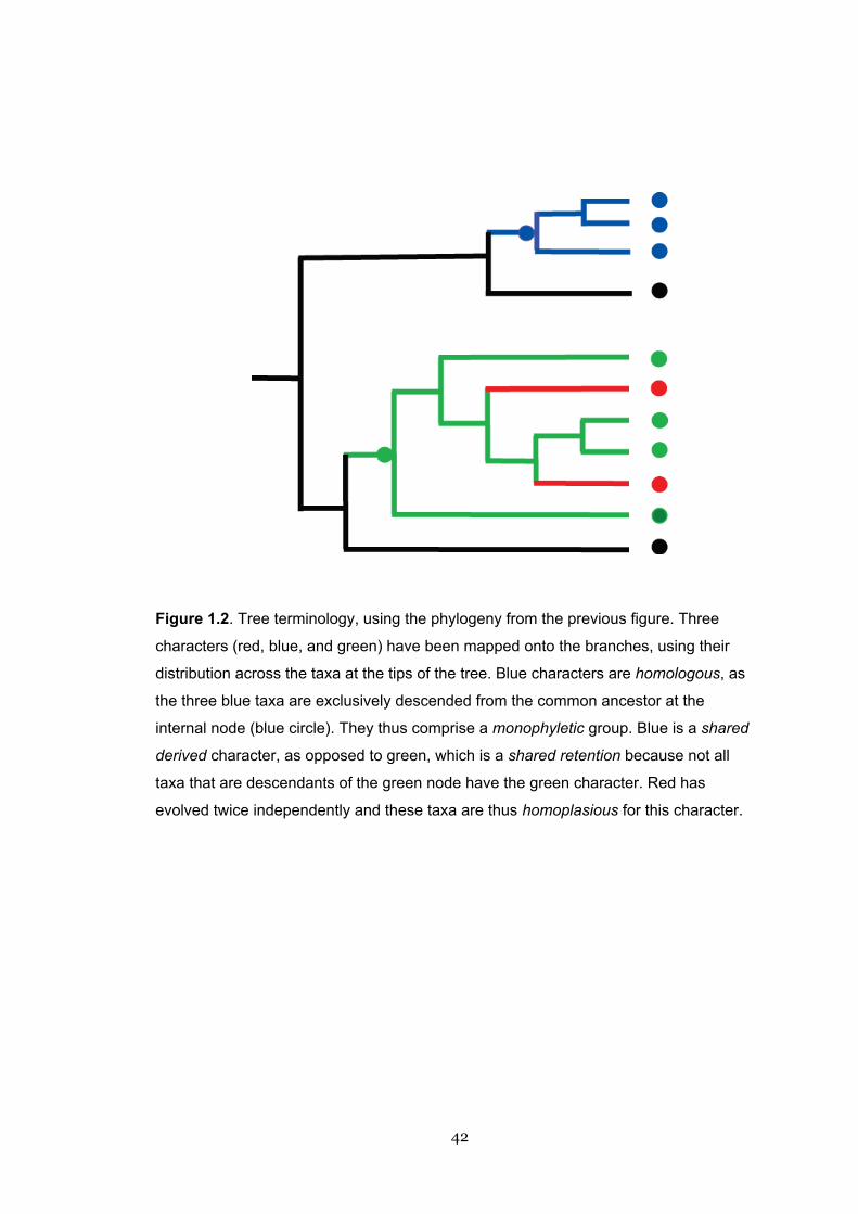
42
Figure 1.2. Tree terminology, using the phylogeny from the previous figure. Three
characters (red, blue, and green) have been mapped onto the branches, using their
distribution across the taxa at the tips of the tree. Blue characters are homologous, as
the three blue taxa are exclusively descended from the common ancestor at the
internal node (blue circle). They thus comprise a monophyletic group. Blue is a shared
derived character, as opposed to green, which is a shared retention because not all
taxa that are descendants of the green node have the green character. Red has
evolved twice independently and these taxa are thus homoplasious for this character.

43
We may also wish to distinguish (i) shared derived traits (also called shared
innovations) that define a group of cultures as the daughter populations of some
exclusive parent, and (ii) shared ancestral traits. Shared ancestral traits are not
usefully informative for hierarchical levels of descent as they can be shared by all or
some daughter populations, as well as by taxa outside the group of interest. With
respect to anthropology, these concerns have also been acknowledged:
A serious weakness of comparative ethnology as an instrument fordoing prehistory is that it has no very reliable way of distinguishingbetween shared resemblances among a set of contemporary culturesthat are due to (a) retention from a common ancestral tradition, (b)convergent development, or (c) diffusion. (Green and Pawley 1999:34)
Thus, “counting cultures” overestimates the number of true innovations of a trait, as
cultures may share traits simply due to being derived from a common ancestral
tradition. Given these problems, what methods have been developed to avoid Galton’s
Problem?
1.4.3 Methods to address Galton’s Problem
1.4.3.1 Sampling methods
Sampling methods, where closely related cultures are excluded from the sample, are
commonly used by anthropologists and are the basis for the Standard Cross-Cultural
Sample (SCCS) of 186 world cultures (Murdock and White 1969) upon which a great
deal of cross-cultural correlation work has been focused (e.g. Ember and Levinson
1991). Historical relatedness is still not controlled for by this method but is merely
pushed back a step, as more distant relationships may account for similarities between
cultural clusters. For example, the SCCS contains three Micronesian cultures (Truk,
Kiribati, and Marshallese) that share many aspects of their common heritage, such as
the presence of matrilineal clans. Thus, sampling methods can return overestimates of
the true number of independent instances of trait evolution, in this case matriliny.
Moreover, this approach results in the loss of information about closely related

44
cultures, the study of which is invaluable for controlled comparison (Mace and Pagel
1994), and leads to Type II errors (false negatives).
1.4.3.2 Controlled comparison
Eggan’s (1954) method examines cultural variation in a small group of closely related
cultures, taking advantage of their shared geographic and ecological background, and
the ability to examine variations within a given type of social structure (e.g. moiety
kinship systems). At this regional level, cross-cultural comparisons are more likely to
focus on appropriately comparable elements (White 1988; Peoples 1993). While some
researchers have proposed that this fine-grained level of analysis may create a new
level of independence among cultures (Borgerhoff Mulder 2001), the problem of
association due to shared inheritance still remains.
1.4.3.3 Autocorrelation
Autocorrelation methods (Dow, Burton, White, and Reitz 1984; Dow 1991) attempt to
remove variation due to spatial proximity and use the residual variance to conduct
cross-cultural analyses. For example, White, Burton, and Dow (1981) used these
methods to examine the causes and consequences of the sexual division of labour in
Africa, finding that 50 percent of the variation in female contribution to subsistence
was explained by the Bantu language family. While these methods may remove some
of the shared variation caused by phylogenetic history, they do not do so with reference
to any explicit evolutionary model (Purvis, Gittleman, and Luh 1994).
1.4.3.4 Phylogenetically controlled comparison
Evolutionary biology avoids the exactly parallel “counting species” problem by
observing phylogenetic history. Over the last 20 years, sophisticated computational
methods have been developed for dealing with the hierarchical relatedness of species
and populations (Felsenstein 2003). These phylogenetic comparative methods are of
two sorts. Tree-building methods, implemented in computer software, construct a
phylogeny from a set of data according to some optimality criterion such as maximum

45
parsimony or likelihood (e.g. Swofford 1999). Comparative methods test for adaptation
and co-evolution whilst taking evolutionary history into account, by mapping traits of
interest onto the branches of a phylogenetic tree (Harvey and Pagel 1991). The details
of these methods and the software used to implement them are described in more
detail in Chapters Two and Three.
Using phylogenetic and comparative methods in anthropology has been
advocated for some time (Ruvolo 1987; Mace and Pagel 1994; O’Hara 1996) but only in
the last few years has a body of work begun to emerge that utilise these methods fully
(e.g. see papers in volumes edited by Lipo et al. 2005; Mace et al. 2005; Forster and
Renfrew 2006). As in evolutionary biology, work has focussed in two areas—applying
phylogenetic tree-building methods to cultural data, and testing adaptive hypotheses
using comparative methods. If cultural diversification proceeds by descent with
modification, it follows that tree methods can be used to explore the underlying
evolutionary processes. Synchronic cultural data on current or archaeological
populations is used to reconstruct hierarchical past relationships by grouping
populations in a nested set of relationships known as a phylogeny or tree. The fit of a
tree model to various data sets can help us understand the relative importance of
phylogenetic (vertical, descent) and ethnogenetic (horizontal, blending) processes in
cultural evolution. Then, by using the phylogeny to control for non-independence and
mapping on our characters of interest, we can make accurate inferences about
correlated evolution. In the next section I describe the first type of phylogenetic
approach: constructing trees (or networks) of evolutionary relatedness from languages
and material culture.
1.4.4 Language phylogenies
In building a phylogeny using language data, aspects of the language system—most
often lexical (word) items but occasionally typological or grammatical features—are
coded and quantitatively analysed in the same way that biologists use molecular or

46
morphological features to build trees of species relatedness. The uses and
implementation of these methods are described in more detail in Chapter Two. To
date, a number of major language families have been investigated using computational
methods: the Austronesian language family of the Pacific (Gray and Jordan 2000;
Greenhill and Gray 2005), the Bantu languages of sub-Saharan Africa (Holden 2002;
Rexova, Bastin, and Frynta 2006), and the Indo-European language family (Ringe,
Warnow, and Taylor 2002; Gray and Atkinson 2003; Nakhleh, Ringe, and Warnow
2005; Rexova, Frynta, and Zrzavy 2003). Other language families are beginning to be
studied with these methods, including Andean (McMahon, Heggarty, McMahon, and
Slaska 2005), Chinese dialects (Ben-Hamed 2005; Ben-Hamed and Wang 2006),
Papuan languages (Dunn, Terrill, Reesink, Foley, and Levinson 2005), Mayan
(Atkinson 2006), and Uto-Aztecan (Ross in preparation).
One measure of the success of these methods in recovering linguistic
phylogenies is demonstrated by the degree to which they agree with established
classifications of historical linguists1 and concur with population dispersal processes
reflected in the archaeological record. For example, Gray and Jordan (2000)
statistically tested an archaeological model of Austronesian colonisation, the “express-
train” sequence, against a maximum-parsimony tree of 77 Austronesian languages.
They showed that the language phylogeny fit the archaeological model far better than
would be expected by chance, and that a competing hypothesis did not. Further
analyses using newer likelihood methods confirmed these findings (Greenhill and Gray
2005). In a similar vein, Holden (2002; Holden et al. 2005) found evidence that a
parsimony tree of Bantu languages corresponded with archaeological models of the
spread of farming across sub-Saharan Africa during the Neolithic and Early Iron Age.
More importantly, the data in these studies has been shown to be as “tree-like” as
1It should be noted that neither agreement or disagreement with previous linguistic classifications should be taken asnecessary and sufficient evidence for the robustness of any particular phylogeny. Different parts of language can displaydifferent patterns of cultural transmission (for example, core vocabulary may be more resistant to borrowing than othervocabulary, or syntax). As such, our expectations of close matches between phylogenies derived from different datasetsmay be variable. I thank A. McMahon for bringing this point to my attention.

47
morphological or molecular data sets of similar sizes by using statistics such as the
consistency index (CI) that determine how well the data fits a tree model (Sanderson
and Donoghue 1989). This indicates that for linguistic vocabulary at least, vertical
inheritance seems to be the predominant mode of transmission.
A common criticism of applying these methods to languages is that languages,
like other aspects of culture, contain some certain amount of horizontally transmitted
items. Words may be borrowed between closely related cultures and between even
cultures in vastly different language families—for example, the English word “taboo”
comes from the widespread (Proto-) Polynesian form *tapu2. In addition, a single
phylogeny may not adequately capture the complex histories of a group of words that
may have evolved along different trajectories, for example, by borrowing. Newer
network methods such as NeighbourNet (Bryant and Moulton 2004; Huson and
Bryant 2006) have been applied to languages and these methods relax the bifurcating
restriction of a branching phylogeny by allowing taxa to connect to more than one
other group, identifying the degree and nature of reticulation and homoplasy in the
data set. For example, Ben-Hamed (2005) represented Chinese dialect patterns with
these methods, McMahon et al. (2005) used networks to suggest that contact
explained similarities in Quechua and Aymara basic vocabulary, and Bryant et al.
(2005) demonstrated how network methods could be used to investigate the degree of
tree-like evolution in Indo-European languages.
1.4.5 Material culture phylogenies
Phylogenetic methods have also been applied to both present-day and archaeological
material culture items (Collard and Shennan 2000; O’Brien, Darwent, and Lyman
2001; Shennan and Collard 2005). In these studies, variation in artefacts is used to
construct a tree of the artefacts themselves or of the populations that constructed
2 An asterisk (*) before a word denotes a linguistic reconstruction for a proto-language.

48
them. For example, O’Brien et al. (2001) reconstructed a phylogeny of Paleoindian
projectile points from the southwestern USA. Some artefacts, such as Turkmen carpet
designs (Tehrani and Collard 2002) show a signal of vertical transmission over
horizontal diffusion; phylogenetic relationships accounted for ~70 percent of the
resemblance between woven assemblages of different Turkmen groups. In contrast,
variation in Native Californian basketry motifs (Jordan and Shennan 2003) are
apparently accounted for by a mainly horizontal transmission model as opposed to the
vertical descent relationships of ethnolinguistic groups. Collard and Shennan (2000)
stress that any a priori assumption of ethnogenesis (emphasising horizontal
transmission processes) needs to be replaced by a case-by-case assessment of the
importance of phylogenetic processes in cultural evolution, as they did for Merzbach
pottery assemblages (2000) and for material culture variation on the north coast of
New Guinea in their 2005 reanalysis of Welsch et al. (1992).
1.4.6 Comparative tests of cultural hypotheses
Comparative methods proceed by mapping traits of interest onto a phylogeny to test
for significant associations while controlling for history. Type I errors of non-
independence (Galton’s Problem, above) are thus avoided as we count only
independent instances of change across the phylogeny (Figure 1.1). Before language
phylogenies using computational methods became available, workers employed the
available classificatory trees of languages (Ruhlen 1987) or worldwide genetic trees
from Cavalli-Sforza et al. (1994) as simple phylogenies of human cultural groups, and
used these to test adaptive hypotheses about gene-culture co-evolution. For example,
Mace and co-workers found that polygyny is associated with male-biased inheritance
(Cowlishaw and Mace 1996) and that increased dependence on agriculture is
associated with higher fertility (Sellen and Mace 1997). Holden and Mace showed that
the evolution of lactose tolerance followed the keeping of livestock (1997), and that
human sexual dimorphism is reduced in populations with greater female contribution

49
to subsistence (Holden and Mace 1999). Other studies have examined correlates of
kinship and marriage variables in East African societies (Borgerhoff Mulder et al.
2001; Moylan, Borgerhoff Mulder, Graham, Nunn, and Håkansson et al. 2006).
Most early studies used parsimony-based comparative methods such as the
concentrated changes test (Maddison 1990) and the method of independent contrasts
(Felsenstein 1985; Purvis and Rambaut 1995) to test hypotheses. Comparative
methods have become more sophisticated in the last few years and now there are
Bayesian (statistical) likelihood methods that allow uncertainty about both the tree
topology and the model of evolution to be incorporated into these analyses (Pagel
1999a). Most recently, tests of adaptive hypotheses have utilised the statistically-
derived language phylogenies (or statistical samples of phylogenies) described above in
combination with modern likelihood-based phylogenetic comparative methods.
Examples follow.
1.4.6.1 Matriliny and cattle in the Bantu
In an evolutionary context, sex-biased inheritance occurs when parents invest
preferentially in one sex over another through the allocation of resources. Holden and
Mace (2003, 2005) investigated patriliny (male-biased inheritance) and matriliny
(female-biased inheritance) in Bantu societies using comparative methods. Using a
phylogenetic tree of 68 Bantu languages as a model of population history (Holden
2002), they tested the hypothesis that patriliny co-evolves with pastoralism, and that
matriliny is lost when cultures adopt pastoralist subsistence. Using the likelihood-
based method of Discrete (Pagel 1994), they constructed an evolutionary flow-
diagram, showing the most probable pathway was that non-cattle-keeping populations
acquired cattle and then switched to patriliny, while cattle-keeping populations were
very unlikely to become matrilineal. In Africa, cattle represent significant movable and
defendable wealth, and as male reproductive variance is higher than female,
investment in sons through the transfer of movable wealth is likely to increase
reproductive success (Holden, Sear, and Mace 2003).

50
1.4.6.2 Worldwide sex ratio and marriage costs
Sex ratio at birth varies worldwide, and may reflect the different costs and benefits of
producing male versus female babies in different environments (Trivers and Willard
1973). Mace, Jordan, and Holden (2003; Mace and Jordan 2005) investigated the
global variation in sex ratio at birth (SRB), testing the hypothesis that SRB correlated
with other demographic variables such as fertility and mortality. We used a genetic
phylogeny based on Cavalli-Sforza et al. (1994) for Old World countries containing a
major ethnic group represented on the tree. The program Continuous (Pagel 1997) was
used to detect correlated evolution in continuous demographic traits. Additionally, the
scaling parameter lambda was used to assess if the traits were evolving in a
phylogenetic manner. With phylogenetic correction for the non-independence of
societies, Mace et al. found that in countries where SRB was skewed towards girls,
fertility and mortality were higher. As the costs of producing and raising boys may be
higher than girls (Wells 2000), in countries where fertility is high the cost-benefit
differentials may be greater and may thus be affecting a small skew in the SRB towards
female babies.
A further comparative analysis examined the correlation of SRB and the costs
of sex-specific marriage transfers (Mace and Jordan 2005). Bridewealth means that
sons will be more costly, while dowry means that daughters will cost more, adding
another variable to the cost-benefit trade-off. Although a standard correlation across
cultures would have shown that marriage payments and SRB were evolving together, a
phylogenetic correlation did not return a significant association between the two traits.
Sex ratio in adulthood (male-biased) was associated with the presence of bridewealth,
indicating that men are competing for brides and thus need to pay for them, but this is
a demographic interaction rather than an example of gene-culture coevolution. In all
the tests, the lambda parameter was shown to be greater than zero, indicating a need
for phylogenetic control in the analyses.

51
1.4.6.3 Marriage transfers in Indo-European societies
Fortunato et al. (2006) investigated variation in marriage transfers (bridewealth and
dowry) in 51 Indo-European societies. Using lexical data, they constructed a Bayesian
sample of language phylogenies. This set of 1000 trees contained differing tree
topologies in proportion to their likelihood, which meant that uncertainties about the
“true tree” were addressed. They used the maximum-likelihood method of Pagel (1994)
in a Bayesian context (Pagel et al. 2004) to estimate the ancestral state of marriage
transfers in Indo-European societies. By reconstructing the ancestral state of each trait
at a given node as a posterior probability, rather than the present/absent/equivocal
states reconstructed in parsimony methods, their methodology identified which trait
reconstructions could be regarded as stable inferences. Results indicated that dowry,
while rarer in present-day societies, was likely to have been the ancestral state, with
bridewealth evolving at least four separate times in the Indo-European family. Further
work on this sample using co-evolutionary tests in the same Bayesian context has
demonstrated that polygyny and bridewealth, and monogamy and dowry, appear to be
evolving together (Fortunato and Mace, in press).
1.4.7 Objections to phylogenetic and comparative methods
What are the dangers of forcing the phylogenetic model onto cultural data? Some of
the objections to studies of cultural evolution in general (§1.3.2) are argued to apply
especially to the phylogenetic approach. Some critics have argued that rapid
evolutionary change, reticulation (borrowing), and cultural recombination all violate
the assumptions of a unique branching pattern characterising a group of cultures
(Bateman et al. 1990; Terrell et al. 1997; Borgerhoff Mulder 2001). However, these are
not so much barriers to the use of phylogenetic models as they are empirical questions
to be tested with different data sets. For example, phylogenetic methods allow us to
assess the appropriateness and fit of a tree model to our data with tools such as
consistency indices and bootstrapping methods.
52
Moreover, a unique branching pattern does not have to characterise all cultural
traits in order for us to investigate cultural evolution; different patterns may exist for
“core” and “periphery” traits (Boyd et al. 1997), and may be compared in the same way
that biologists compare “gene trees” and “species trees” (Pamilo and Nei 1988; Page
1998). Some authors have suggested that we should be tracing the unique phylogenetic
histories of different traits rather than constructing population histories using
languages or material culture as a proxy for ethnolinguistic populations (Pocklington,
McElreath, and O’Brien 2005). Studies of this type, employing “iterated” (McElreath
1997) or “perfect” (Nahkleh et al. 2005; Ringe et al. 2002) parsimony, attempt to
remove homoplasious traits from the data and retain only those with clear branching
lineages. However, there is substantial loss of information inherent in such
approaches, and if we are interested in questions about (for example) rates of
evolution or adaptation, we proceed most profitably by plotting traits of interest on a
background of evolutionary relationships, even if that phylogeny is only an imperfect
model of history.
Relatedly, while discriminating vertical from horizontal transmission can be
crucial in determining some processes of cultural diversification, in the context of
testing for adaptation, a borrowed trait counts as an instance of adaptation just as
much as if the trait was invented along a lineage. As long as a trait is adopted by
“choice”, not imposed by force (Durham 1991) or acquired as a side-effect of some
other complex of traits, the acquisition through borrowing or contact should be
another independent instance of adaptive cultural change (Mace and Pagel 1994). To
disregard borrowings in adaptive tests is unreasonably conservative.
Borgerhoff Mulder (2001) argues that the need for phylogenetically controlled
comparison is still an open question, and that while broad global patterns of trait
distribution (such as modes of marriage) may retain an historical signal, at a more
fine-grained local level natural or cultural selection pressures may act on traits to
produce a new level of independence among related populations. Cashdan and Rogers
53
(1997) have also argued that comparative methods lack statistical power by decreasing
the number of data points available for analysis. This is however a misconception of
the concept of power, as the number of significant correlations found in non-
phylogenetic analyses will contain some amount—unknown until phylogeny is
controlled for—of Type I error (Mace 2005). Borgerhoff Mulder et al. (2001) examined
the need for phylogenetic control in a study of local variation in East African kinship
and marriage. They compared phylogenetically controlled analyses to standard
correlations for each of their 36 hypotheses. Of these, 21/36 were non-significant
under both types of methods, 5/36 were significant under both types, 8/36 were
significant under conventional correlations but not when phylogenetically controlled,
and 2/36 were significant when phylogenetically controlled but not under conventional
tests (2001:1072). It is notable that nearly two-thirds of conventionally significant trait
associations disappeared with phylogenetic control, indicating a definite need for this
kind of analysis where possible.
In their discussion and elsewhere, Borgerhoff Mulder and colleagues argue that
comparative methods are conservative tests and these results, like other phylogenetic
tests, are not showing two types of important adaptive processes. Firstly, comparative
methods focus on the origins of adaptive trait associations to the exclusion of
evolutionary forces maintaining an association between traits (stabilizing selection).
Secondly, comparative methods mask the effect of habitat selection, where closely
related groups move into similar environments (Borgerhoff Mulder 2001). However,
both points, sometimes under the rubric of “phylogenetic inertia”, are recognized in
comparative biology (Orzack and Sober 2001); likelihood methods that allow the
direction and order of evolutionary change to be determined can address
origin/maintenance questions (e.g. Pagel 1994), and the points above do not constitute
grounds for not using an historical method when one is available.
On the issue of phylogenetic inertia, stability or lability in cultural traits cannot
be assumed at the outset. If a trait is shared by many closely related cultures, it does

54
not necessarily imply that evolution is weak, as there may be a good adaptive reason to
retain the trait. By mapping traits onto a phylogeny we can show that many aspects of
culture show a remarkable time-depth, for example, the practice of dowry can be
reconstructed for the root of the Indo-European tree, a time depth of approximately
6,000 years (Fortunato et al. 2006). Even traits without clear adaptive function may
demonstrate considerable variation in lability. Marck (1996) compared the names and
functions of the first-order anthropomorphic Polynesian gods against the background
of phylogeny provided by Polynesian languages. While some types of gods could be
traced to their Proto Nuclear Polynesian ancestor e.g. *Tuu, god of war (1996:247),
suggesting a cultural stability of over 2800 years, others had gone through changes in
function, in name, and in importance even in closely related cultures. For example, the
sea god Tangaroa is a first order deity in Mangarevan society, but in the closely related
Marquesas, thought to have diverged less than 800 years ago (Kirch and Green 2001),
Tangaroa was reduced to a 39th-generation offspring of the gods and accorded no great
importance.
1.4.8 Simulations
By far the most common objection to the application of the phylogenetic model to
cultural data is the (unquantified) presence of horizontal transmission between
societies. Some workers have used simulation studies to address the impact that
differing levels of horizontal transmission have on (i) recovering phylogenies, and (ii)
accurately testing for correlated evolution. Atkinson, Nicholls, Welch, and Gray
(2005) modelled the effects of increasing levels of horizontal transmission in a
linguistic data set on the ability of tree-building methods to estimate the divergence
date (time depth) of a phylogeny. As well as modeling random horizontal transmission,
they used a spatially realistic model of evolution where borrowing was much more
likely between closely related as well as spatially close languages. They found that

55
borrowing levels of 20 percent—a significant amount of vocabulary—only altered
estimates of divergence time by, at most, 500 years from an 8500 year time depth.
Nunn et al. (2006) simulated the co-evolution of two traits in a spatial grid and
calculated Type I error rates under conventional correlations and the phylogenetic
method of independent contrasts. Under differing conditions of extinction and spatial
configuration, they found that phylogenetic methods always outperformed
conventional correlations. By varying the level of horizontal transmission in the
simulation they were able to show that small amounts of horizontal transmission
increased the Type I error rates of phylogenetic method; however, in all analyses the
phylogenetic method outperformed conventional correlations (2006:193). It is
important to note that this study used a parsimony-based comparative method. These
methods have been shown to perform poorly when multiple changes may take place
along a lineage and when rates of evolutionary change are high (Felsenstein 2003).
Likelihood-based or Bayesian methods that use the information contained in branch
lengths, and incorporate a more explicit model of evolution may not be as affected by
horizontal transmission.
Both simulation studies investigated the impact of increasing levels of
horizontal transmission on the two broad types of phylogenetic approaches to cultural
evolution, tree building and comparative tests. In a survey of work published to date,
Collard, Shennan, and Tehrani (2005) took an empirical approach to determine the
relative importance of vertical and horizontal processes. They reviewed nine studies
that had used phylogenetic methods on cultural data (language, and archaeological
and material culture artefacts) and compared the tree-statistics derived from these
analyses with 21 biological analyses of molecular, morphological, and behavioural
data. By comparing the retention index (RI), which is a measure of the fit of the data to
a tree model where 1 indicates a perfect fit, Collard et al. tested the expectation that
cultural data sets would show more evidence of horizontal transmission and so be less
tree-like, thus having a lower RI, than the comparable biological data sets. Their

56
results showed that the cultural data sets actually had the same mean RI (0.60) as the
biological data sets, although the range of RI was wider for the cultural analyses.
Although it is true that tree-building programs will produce a tree regardless of the
degree of vertical signal in the data, statistics such as these indicate that for the small
amount of empirical work published, vertical transmission of cultural traits is
apparently important. As well, horizontal transmission is not so endlessly reticulate as
to render phylogenetic methods unusable, as has been suggested by some critics
(Moore 1994; Terrell et al. 2001). More importantly, most workers have now realized
that the production of a tree from a set of data is only the first step (Borgerhoff Mulder
et al. 2006); a phylogeny is a hypothesis about evolutionary relationships—a model of
population history—and can be used in conjunction with independent data sets to
examine the pattern of cultural evolution.
1.4.9 Different lines of evidence
The use of different types of data to investigate questions of human prehistory is an
approach that Kirch and Green (2001) have termed “triangulation”. Their methodology
involves the use of historical linguistics, comparative ethnography, and archaeological
data to make inferences about the past, drawing on all available information to paint a
complete picture of cultural evolution and diversity. Prehistoric human migrations
associated with a Neolithic agricultural dispersal (Bellwood 1996a, 1996b; Bellwood
and Renfrew 2002; Diamond and Bellwood 2003) appear to have resulted in cultural
groups with a meaningful degree of biological and cultural continuity through time and
space. Although this continuity is not a necessary requirement for the use of
phylogenetic approaches, it facilitates the use of different lines of evidence (e.g.
biological, linguistic, ethnological, archaeological) to address the same questions, as
they are geographically and historically framed together. We cannot assume that
agricultural peoples always expand and migrate because of their technological
innovations and/or population pressure: sometimes agriculture has allowed people to
57
“stay at home” (Campbell 2002) and consolidate their presence in already-occupied
territories, such as may be the case for Mixe-Zoquean (Olmec) languages (Hill 2001).
However, general consensus holds that the Austronesian language family of the Pacific
region is clearly one such example of a agriculturally-motivated Neolithic dispersal
(Diamond and Bellwood 2003), and as such, provides an excellent case study for these
combined approaches.
Additionally, regional rather than worldwide studies are preferred in
comparative anthropology (Eggan 1954). Firstly, the focus is on a lesser time depth,
allowing us to use language relationships to build a model of population history.
Secondly, we are likely to being comparing “like with like” in regional studies; that is,
making appropriate comparisons and inferences about the types of cultural traits
under study. Thirdly, the problem of isolates (both linguistic and genetic), and the
uncertain relationships of human populations at the base of any worldwide tree render
a phylogenetic model in the global context more problematic. In the next section I
present the ethnographic context for the specific regional case that was studied in this
thesis.
1.5 The ethnographic context: Austronesian cultures of the Pacific
1.5.1 Summary
This section describes the regional focus for the thesis, the Austronesian cultures of the
Pacific. The prehistoric colonisation of the Pacific and current models of Austronesian
dispersal are reviewed. Molecular anthropological findings from mtDNA and
Y-chromosomal markers show differing pictures, possibly due to sex-specific
migration patterns. Although the “island laboratory” model is now considered
inadequate, previous work in the region has used evolutionary concepts such as
adaptation. Variation in descent rules and post-marital residence patterns may reflect
adaptive evolution in kinship systems. Austronesian societies vary in their kinship
58
organisation but the evolution of these traits is not well understood, thus, the thesis
will test co-evolutionary hypotheses on the evolution of matriliny and reconstruct
ancestral states of descent and residence patterns. The chapters are described in brief.
1.5.2 Pacific colonisation
Prehistoric human expansion into the Pacific took place over the last 60,000 years
(Kirch 2000). Pleistocene hunter-gatherer populations from Southeast Asia crossed
open water to colonise Sunda—Australia and New Guinea, connected by lowered sea-
levels (Spriggs 2000)—by around 56,000 BP (Roberts et al. 2001), reaching the
Bismarck Archipelago by 39,500 BP (Leavesley et al. 2002) and Buka in the Solomon
Islands by 29,000 BP (Wickler and Spriggs 1988). Further migrations may have
followed, as the area from Island Southeast Asia through to the Solomons—Near
Oceania (Green 1991)—constituted what Irwin (1992) has termed a voyaging nursery,
with calm weather and undemanding sailing conditions. The descendants of these
people are dispersed throughout New Guinea and parts of Island Melanesia (Figure
1.3); they speak a diverse range of languages—“Papuan” or Non-Austronesian
(NAN)—whose heterogeneity indicates a long time depth in the region (Foley 2000).
Here they are referred to as “indigenous Melanesians”, following Hurles et al. (2002).
By 9000 BP there is evidence for tree-crop cultivation in highland New Guinea (Golson
1991), but not intensive agriculture or high population density in the region.
The environs of southern China have been identified as a center of early
agriculture (Diamond and Bellwood 2003), and many Asian language families such as
Tai-Kadai and Hmong-Mien have their deepest roots in this region (Benedict 1975;
Bellwood 1996a). The Austronesian (AN) language family also derives from this region,
with its highest diversity—nine of ten first-order subgroups—centred on Taiwan (Blust
1984-5; Pawley and Ross 1993; Blust 1999). An agricultural dispersal model involves
the movement of Neolithic peoples out of Taiwan around 4500–6000 BP, carrying with
them newly developed agricultural technology and domesticates, and speaking

59
Austronesian (AN) languages (Bellwood 1985, 1997, 1991; Blust 1985, 1995, 1996;
Pawley and Ross 1993; Bellwood, Fox, and Tryon 1995; Pawley 1997; Spriggs 1997,
2000). From Island Southeast Asia, AN speakers moved through the Pacific,
overreaching the extent of the existing populations to colonise the uninhabited regions
of Remote Oceania, the islands of Micronesia and Polynesia (Figure 1.3). The AN
family numbers some 1200 languages and its speakers are dispersed over half the
circumference of the Earth, from Madagascar to Easter Island (Tryon 1995) (Figure
1.4).

Figure 1.3. Map of the Pacific showing geographic and culture areas. Conservative dates (years BP) of AN archaeological settlement in key areas are shown in
green, from Hurles et al. (2002) and Kirch (2000). The traditional classification of Melanesia, Micronesia, and Polynesia are used primarily as geographic
designations; in preference we use Near and Remote Oceania (Green 1991). Near Oceania denotes areas settled before the Lapita horizon c. 3300 BP, where
islands are for the most part intervisible. Remote Oceania denotes areas uninhabited by humans before Lapita, predominately far-flung islands.
60

Figure 1.4. Map of the Pacific showing the extent of the Austronesian language family. The boundaries of high-order AN subgroups are indicated
and their branching patterns are shown in the top right-hand corner. Non-Austronesian (NAN) languages are spoken in most of New Guinea and
on some off-shore islands. Different language families are present in Australia and Mainland Southeast Asia. The grey arrow-paths trace the
approximate direction of the Austronesian expansion.
61

62
1.5.3 Austronesian languages
Early European travellers in the Pacific such as Captain Cook observed word
similarities between far-flung languages like Tahitian and Malay. Early work by
Dempwolff (1934–1938) characterised the rough outline of the AN language tree,
grouping closely related languages together and tracing them back to a putative
“mother-tongue”, Proto Austronesian. Historical linguistics proceeds by a
“comparative method” comparing cognate terms (words assumed to have a common
origin) across languages and working out regular sound correspondences (Trask 1996;
Crowley 1997). These correspondences are then used to establish the directionality of
change in language and to reconstruct proto-vocabulary. The method is recursive in
that each new cognate examined refines the subgrouping hypotheses, confirming (or
not) the placement of a language in the family hierarchy. Careful comparative
reconstruction is an ongoing endeavour by Pacific scholars, and on the basis of this
work Blust (n.d.) and Tryon (1995) have collated large comparative dictionaries of AN
languages.
1.5.3.1 Austronesian subgrouping
Blust (1998, 1999, in preparation), synthesizing work across the discipline as well as
his own, and others (Pawley 1997; Tryon 1995), have described the internal
subgrouping of Austronesian. The high-order subgroups of AN are primarily Formosan
(9/10 are found on Taiwan), with one branch forming the rest of the family, Malayo-
Polynesian (MP). MP then splits into Western (WMP) and a Central-Eastern branch
(CEMP). The WMP languages, which include those on the Philippines, Borneo,
Sumatra, Java, Sulawesi, and parts of Indonesia, are not considered a true (exclusive)
innovation-defined group, but rather are a catch-all for non-CEMP languages (Ross
1997). CEMP splits into Central (languages on the islands of Timor, the Lesser Sundas,
and Maluku), which is also considered innovation-linked rather than defined (Blust
1993b) and an Eastern branch (Blust 1978). This Eastern branch splits into South

63
Halmahera-West New Guinea, comprising languages around the Bird’s Head of Irian
Jaya and Halmahera (SHWNG), and the large Oceanic (OC) group. The Oceanic
subgroup is well defined as a whole but is possessed of a “rake-like” high-order
subgrouping rather than a bifurcating family tree structure.
Figure 1.5. Subgrouping of the Austronesian language family. Taken from Tryon
(1995), Pawley (1999), and Blust (in preparation). Formosan languages are spoken on
Taiwan. The WMP and CMP subgroups are not clearly innovation-defined, that is, they
are a residual collection defined by their exclusion from another branch (Proto Central-
Eastern and Proto Eastern Malayo-Polynesian, respectively).
64
Dialect networks, or chains, form when language communities maintain
overlapping ties with each other for an extended period of time before (if ever)
diverging completely (Ross 1997). In a phylogenetic context, words will not have
unique branching histories, and trees will appear to have low resolving power at nodes
representing parts of a dialect chain. Dialect diffusion may in fact be ubiquitous
through the whole of the higher-level subgrouping of AN languages reflecting (i) the
speed of the AN expansion through Island Melanesia and/or (ii) the maintenance of
dialect networks over the voyaging-corridor area (Pawley 1997; Green 1999).
1.5.4 The Austronesian dispersal
Linguistic, archaeological and biological evidence gathered by Pacific scholars over the
last fifty years has been used to argue a number of different scenarios for the
Austronesian colonisation of the Pacific. Historical linguistics in particular has been
important in establishing the internal relationships of Austronesian-speaking
populations, and through cross-talk with archaeologists, linguists have been able to
correlate language sub-families with particular archaeological horizons (e.g. Shutler
and Marck 1975; Pawley and Green 1984; for Proto Oceanic and the Lapita horizon in
the Bismarck Archipelago). In addition, by reconstructing proto-vocabulary for a
putative prehistoric period, linguists can corroborate the archaeological record (e.g.
the POC term for a particular fish lure, *bayan) and can supply information where
none might be archaeologically available, as in the case of the Proto Polynesian lunar
calendar (Kirch and Green 2001).
All modern workers agree that Pacific peoples had their ultimate roots in Asia,
but disagree as to the timing, speed, and degree of intermixing between populations. A
mainstream archaeological consensus (Bellwood 1997; Kirch 2000; Green 2003) for
the geographic spread of speakers of AN languages might proceed roughly as follows.
People from Taiwan moved into Island Southeast Asia through the Philippines at
approximately 4200 BP with early “red-slip” pottery, taro and yam horticulture,

65
chickens, and outrigger canoes, penetrating south and easterly into Wallacea. From the
Philippines, people moved through Borneo to Nusa Tenggara, later spreading to
Madagascar and the Malaysian peninsula. Others migrated south-easterly through
North Sulawesi, the Moluccan Strait and Banda Sea. In Island Southeast Asia, it
appears that AN languages replaced those of the indigenous cultures (Adelaar 1995). It
is unclear to what degree these new populations initially practiced intensive
agriculture (Spriggs 1997). After a pause, from this Wallacean region AN speakers
spread quickly through Halmahera and around Cenderawasih Bay (Irian Jaya), along
the north coast of New Guinea to the Bismarck Archipelago. These people carried their
AN languages as part of the “Lapita Cultural Complex” as far as the Solomon Islands,
Vanuatu, and New Caledonia by 3300 BP (Specht and Gosden 1997).
Lapita, named after a decorated pottery style, appears as an archaeologically
distinct package consisting of animal and horticultural domesticates, over-water stilt
houses, characteristic fishing technologies, outrigger canoes, personal adornments,
and other items of material culture (Kirch 1997; Spriggs 1997; Green 2003). Lapita
sites first appear in the Bismarck Archipelago around 3300 BP and quickly spread to
Fiji, Tonga, and Samoa (Western Polynesia) by 2950 BP (Anderson 2002; Spriggs
2000). Some Lapita pottery features show continuity with earlier AN Neolithic sites,
such as the Ta-p’en-k’eng and then Yuan-shan pottery assemblages in Taiwan, thus
supporting a descent relationship from Asian traditions (Chang and Goodenough
1996; Bellwood 1997). Other features of the Lapita complex, such as tree crops, suggest
these items come from integration with indigenous Melanesian societies (Denham
2004).
Expansion further into Remote Oceania may be linked with atoll emergence
through sea-level drops around 2000 BP (Nunn 1994). Lapita descendants expanded
northerly up to Central and Eastern Micronesia around 2000 BP, possibly from the
Vanuatu region (Intoh 1997). In Western Polynesia, an archaeological “pause” of
~1000 years is evident before the attested dates of 1700–1200 BP in the Marquesas
66
(Central/Eastern Polynesia), with the far corners of the Polynesian triangle—Hawai’i,
Rapa Nui (Easter Island), and Aotearoa (New Zealand)—being settled around
800–1000 BP (Spriggs and Anderson 1993; Bellwood 1997; Kirch 1997; Green 1999;
Burley and Dickinson 2001; Kirch and Green 2001; Anderson 2002).
1.5.5 Models of colonisation
1.5.5.1 Express train/Out of Asia
According to the “express train to Polynesia” model (Diamond 1997; Diamond 1988),
the AN expansion from the Taiwanese homeland was a swift and relatively
encapsulated event. Following other Neolithic farming expansion models (Renfrew
1987), on this model the Austronesians were propelled by a successful package of
technological inventions—rice cultivation from China and then horticultural and
sailing technologies from Island Southeast Asia. On leaving Taiwan around
approximately 4500 BP, Austronesian speakers took only 1500 years to reach the edges
of Western Polynesia—a distance of 10,000 kilometres (Bellwood 1978). Under this
hypothesis, genetic mixing with indigenous Melanesians was minimal, although it has
occurred since. Green (2003:5) notes that the “metaphor of a train journey…” should
by now be “rendered suspect”, but that its persistence in the literature is largely due to
molecular biologists wishing to test simple predictive models.
1.5.5.2 Entangled bank
In contrast, a minority group of workers dispute the adequacy of the agricultural
dispersal model at all for explaining the distribution of AN-speaking Lapita people
throughout Oceania (Terrell et al. 1997, 2001). In the past this perspective has been
associated with an indigenous Melanesian origin of the Polynesians (Clark and Terrell
1978; Allen and White 1989). Often vague with respect to testable assertions, these
workers have offered no viable alternative model beyond 45,000 years of ongoing
interaction in Near Oceania (Terrell 2001:107). Both this position and the strong

67
claims for speed and isolation made by the “express train” model represent extreme
ends of a continuum embodying ethnogenesis and phylogenesis in population history
(Jordan and Gray 2001). Intermediate scenarios exist and are more likely to capture
the complex population history of the area. These scenarios have been stimulated in
part by new genetic data.
1.5.6 Molecular anthropology in the Pacific
The last 15 years have seen heated debate concerning the origins, timing, and degree of
AN–NAN interaction, stimulated in part by new genetic evidence from molecular
anthropology. Most of these studies have used uniparental loci: mitochondrial DNA
(mtDNA) inherited through the maternal line, and the non-recombining portion of the
Y-chromosome inherited through males. Both these loci are non-recombining and
have small effective population sizes, increasing the likelihood of drift and population
differentiation over short periods of time. They can thus be more suitable than nuclear
loci for tracing population histories in a regional context.
1.5.6.1 Mitochondrial DNA
High frequencies of a nine base-pair (bp) mtDNA deletion in the COII/tRNALys region,
and characteristic motifs in the mitochondrial control region, are present in Polynesian
populations (Melton et al. 1995; Redd, Takekazi, Sherry, McGarvey, Sofro, and
Stoneking 1995; Sykes, Leiboff, Low-Beer, Tetzner, and Richards 1995). The
precursors of this “Polynesian motif” can be traced back to Island Southeast Asian
populations including Taiwan, but these lineages are virtually absent from NAN-
speaking populations in New Guinea and Island Melanesia (Lum and Cann 1998;
Merriwether, Friedlaender, Mediavilla, Mgone, Gentz, and Ferrell 1999). Lack of
indigenous Melanesian mitochondrial lineages in Polynesia also implies little female
genetic admixture. The 9bp deletion is also found in mainland East Asian populations,
confirming the “Out of Asia” scenario for the ultimate origins of the Austronesians. By

68
estimating the time to the most recent common ancestor (MRCA) of the Polynesian
motif, Oppenheimer and Richards (2001a, 2001b) postulate the AN expansion to have
derived from Eastern Indonesia during the Pleistocene (~17,000 BP) rather than
Taiwan. However, this interpretation—the “Slow Boat”—remains contentious, due to
wide confidence intervals on the coalescent time (5500–34,500 BP) and the direct
conflict of these conclusions with the significant body of linguistic evidence. Moreover,
further work shows that Indonesian mtDNA sequences are consistent with a MRCA
during the Holocene (Cox 2005).
1.5.6.2 Y-chromosome lineages
A more complex picture has emerged from studies of Y-chromosome haplotype
diversity. A pre-Holocene, indigenous origin for a majority of Oceanic and Southeast
Asian Y-chromosome lineages was argued by Capelli et al. (2001) on the basis of the
distribution of haplogroup C, coalescing at >12,000 BP across the region. Other studies
have similarly found that while all Pacific-region Y haplotypes appeared to ultimately
originate in Asia, the proximate origins of Polynesian Y-chromosomes are
predominantly indigenous Melanesian (Kayser et al. 2000; Hurles et al. 2002). The Y-
chromosome genetic patterns of Oceanic populations may concur with the general
sequence of the “express train” model (Hurles et al. 2002), but show evidence for
much more interaction with indigenous populations in Eastern Indonesia and
Melanesia along the way than is suggested by that earlier model. A lack of both
Taiwanese- and Melanesian-specific Y-chromosome lineages in a Cook Island
(Polynesian) population (Su et al. 2000) shows how founder effects and drift may
complicate analyses and highlights the need for widescale sampling.
1.5.6.3 Autosomal markers
Some nuclear loci, usually short tandem repeats (STRs), have been used in Pacific
molecular anthropology. Lum and Cann (2000) used neutral autosomal loci as well as
mtDNA to evaluate genetic distances between Pacific Island and Asian populations.

69
mtDNA distances suggested that Micronesians and Polynesians originated in Island
Southeast Asia, but autosomal distance markers suggested substantial, ongoing male
gene flow of Remote Oceanic populations with indigeous Melanesians in Near Oceania.
Correlating autosomal genetic distances with geographic and linguistic distances
showed a similar pattern (Lum et al. 2002).
1.5.6.4 Sex-specific patterns of dispersal
Y-chromosome and mtDNA patterns tell the histories of male and female movements.
Approximately 70 percent of societies practice patrilocal residence, that is, women
move to their husband’s kin group on marriage (Murdock 1949:38). In comparison,
matrilocal residence involves the movement of men to their wives’ kin group, and is
much less common worldwide. An eight-fold higher migration rate for females
worldwide was claimed on the basis of mtDNA versus Y-chromosome diversity
(Sielstad et al. 1998), although this may only hold regionally (Wilder et al. 2004). Oota,
Settheetham-Ishida, Tiwawech, Ishida, and Stoneking (2001) compared mtDNA and Y
diversity in matrilocal and patrilocal Thai hill-tribe villages. They found that mtDNA
diversity was restricted and Y-chromosome diversity greater in the matrilocal villages,
while the reverse pattern was obtained in the patrilocal societies. Kayser et al. (2003)
found much higher levels of diversity in mtDNA as opposed to Y-chromosomes in Irian
Jaya, attributing this to extreme patrilocality and/or male-biased parental investment
in the region. Hage and Marck (2003) argue that the discordant molecular findings in
the Pacific are best accounted for in a model where Proto Oceanic society was
matrilocal and/or matrilineal, that is, where migrating AN speakers incorporated
diverse males (and their genes) into social groups whilst retaining a restricted,
ancestral set of female-specific genetic markers. These claims are addressed in
Chapters Five and Six.
70
1.5.7 An integrated model
Molecular work, especially the conflicting results from sex-specific markers, can be
integrated into a messier but ultimately more realistic model of Pacific prehistory. The
intermediate “Triple I” (Intrusion, Innovation, Interaction) model (Green 1991, 2003;
Kirch 2000) allows for ongoing interaction—genetically, linguistically and
culturally—between both NAN and AN cultures in a “voyaging corridor” stretching
from Eastern Indonesia through to the Bismarck Archipelago during the middle part of
the AN expansion. The geographical sequence of AN dispersal remains broadly as
described, but a number of “pulse, pause, and step” sequences are proposed. At each
step, specific cultural or technological developments are surmised to have taken place,
such as the appearance of Conus shell ornaments in Proto Oceanic society, or the
integration of crop domesticates from Island Southeast Asia (Green 2003:5).
1.5.8 Later developments in Austronesian history
Monsoon sailing across the Bay of Bengal to Island Southeast Asia led to Indian
trading and subsequent Hindu and Buddhist influence in Indonesia, especially Java
and Bali, from approximately 1700–1500BP, although it took some centuries for this
influence to become established in religious and political institutions (Geertz 1980;
Bellwood 1997). Indianisation appears to have only affected elite institutions and had
little impact on established cultural traditions of the peasantry. Islam, brought to
Island Southeast Asia in early medieval times, spread through an association with
favourable trading and power alliances with native rulers, as well as through
conversion (Kumar 1979, cited in Bellwood 1997). By 500 BP Islamic and Portuguese
influence meant that the Indo-Malaysian Archipelago was part of the greater Asian
world, with emergent Malay sultanates and coastal mini-empires in southern Sulawesi,
such as the Bugis and Makassarese (LeBar 1975).

71
East of Island Southeast Asia, Indian and Islamic impact was not evident.
Societies in both Remote and Near Oceania west of Irian Jaya retained contact and
trade networks, some over large distances—for example, the kula ring in the Massim
Archipelago of Papua New Guinea (Malinowski 1922) and the sawei tribute network in
the Caroline Islands of Micronesia (Lessa 1950)—but were not significantly involved in
the larger Asian world system. European contact and Christianisation, beginning in the
18th century, affected all Remote Oceanic societies to some degree, although most
retained largely traditional lifeways until the Second World War (Denoon 1997).
1.6 Cultural evolution in the Pacific
1.6.1 Islands as laboratories
Goodenough, observing the linguistic and anthropological patterns in the Pacific,
suggested that the advantage of studying cultural evolution in Oceania (i.e. the remote
Pacific Islands) was the limited contact that those societies had with unrelated
traditions. As such, all changes could be seen as elaborations of the parent culture, and
systematic comparisons between populations could reveal important characteristics of
ancestral “proto-cultures” (1957:153). Sahlins famously observed the Pacific islands to
be a sort of cultural laboratory: an “extended series of experiments in cultural
adaptation and evolutionary development … where culture so experiments,
anthropology finds its laboratories—makes its comparisons” (1963:285). Indeed, the
isolation provided by distance in previously uninhabited Oceanic islands might seem
the perfect setting for studies of adaptive radiation (Simpson 1953), without the
complications imposed by frequent contact, borrowing, or warfare. Similarly, Kirch
stated that we might view islands as excellent “theatres” (1980:39) for the study of
human-environment co-evolution. In the Polynesian case at least, a diversity of human
cultural adaptations is derived from a common source population.

72
However, the idealised notion of closed, non-interacting populations on
Oceanic islands has been dispelled by work in the last 25 years. The archaeology of
trade items and raw materials (Weisler 1998), voyaging simulation (Irwin 1992),
studies of borrowing in language and cultural traits (Tent and Geraghty 2004), and
more sophisticated models of genetic interaction (Hurles et al. 2002; Lum et al. 2002)
have shifted thinking away from the island laboratory model. Pacific peoples saw the
ocean as a pathway, rather than a barrier, to interaction (Peoples 1993), although long-
distance voyaging declined in Remote Oceania in the last 600 years (Rolett 2002). In
addition, for Austronesian societies in Island Southeast Asia the island laboratory
model has never been suggested; it is thus not appropriate to apply such a metaphor to
the family as a whole.
1.6.2 Evolutionary approaches
A range of ecological environments is present in the Pacific: semi-continental
landmasses, continentally derived islands, volcanic (“high”) islands, and coral atolls
(Thomas 1963). Across this range of environments, Austronesian-speaking peoples
display significant variation in cultural diversity. For a number of years, evolutionary
concepts have been used to describe this diversity (Goodenough 1957; Goldman 1970;
Alkire 1974; Kirch 1984). Drift and founder effects have been used to describe the
attenuation of linguistic forms from West to East across the Pacific (Elbert 1953; Blust
1981a). Frequently, aspects of social life have been described as adaptations to aspects
of the environment. Sahlins (1958) examined levels of social stratification in Polynesia
as adaptive responses to spatial and ecological features of atolls versus high islands.
Extending this, Kirch (1980) modelled increases in social stratification as the outcome
of population pressure and shifting cultivation. In the Caroline Islands, matrilocal
residence and dispersed family settlements were related by Alkire (1974) to a pattern
of multiple-crop subsistence; when economies were concentrated on a single crop
other forms of social organisation emerged.

73
These authors and others (Hainline 1965; Goldman 1970; Kirch and Green
1997) viewed Oceanic and Polynesian societies as especially suited for comparative
analysis because they represented closely related elaborations of a common ancestral
tradition. Kirch and Green’s reconstruction of Ancestral Polynesian Society is an
exceptional application of the “triangulation” method (2001:42) in historical
anthropology. They control for shared history with language phylogeny, and examine
archaeological and ethno-historical data as well as proto-vocabulary to reconstruct
aspects of ancestral Polynesian social structure, material culture, subsistence, ritual
and ecology. However, theirs is a non-computational phylogenetic approach, without
quantitative hypothesis testing.
Other projects attempt to relate the vocabulary of proto-languages to
archaeological and ethno-historical evidence, for example, the Oceanic Lexicon Project
(Ross et al. 1998, 2003; http://rspas.anu.edu.au/linguistics/projects/oceanic), which
has used the linguistic comparative method to reconstruct aspects of Proto Oceanic
material culture (such as sailing and fishing technology) and the physical world (such
as concepts of time). Unlike material culture, many aspects of past lifeways—especially
social structure—leave no direct evidence in the archaeological record. While some
authors have extrapolated the post-marital residence patterns of past societies from
floor plans of Chaco settlements (Peregrine 2001) such associations are highly
inferential (Schillaci and Stojanowski 2003).
Linguistic reconstructions by analogy with ethnographic examples have been
the primary means with which we can infer the social behaviours of ancestral
Austronesian cultures. For example, Blust (1980) has inferred the existence of descent
groups in the extra-Formosan AN languages. Similarly, Hage (1998) has used linguistic
reconstruction to show how Proto Oceanic society was likely to have had senior and
junior lines of chiefly authority. Building on this base, by using phylogenetic methods
we can now statistically infer the ancestral states of Austronesian social systems, and
test co-evolutionary hypotheses about the distribution of cultural diversity.

74
1.7 Austronesian kinship
1.7.1 Descent
Descent systems delineate which relatives an individual affiliates with most closely
(Murdock 1949). Inheritance, rights and obligations, the regulation of marriage, and
social and material assistance are all affected to some degree by kinship rules that
stipulate who is and is not regarded as part of one’s descent group. Virtually all types of
descent organisation can be found amongst the Austronesian-speaking cultures of the
Pacific (Table 1.2). Even on Taiwan, the consensus homeland of Austronesian
expansion, there exists a diversity of descent systems spanning the range of cross-
cultural variation (Mabuchi 1960). This diversity broadly reflects that seen worldwide
(Murdock 1949) and thus Austronesian societies are a useful regional case with which
to test hypotheses about the evolution of descent. Descent systems fall into two broad
categories (Fox 1967; Holy 1996). Unilineal descent means that an individual is a
member of one, non-overlapping kin group, traced through either their father’s male
ancestors (patriliny) or their mother’s female ancestors (matriliny). Non-unilineal
descent (also called cognatic) occurs when individuals trace kin relationships in
overlapping kin groups, and can be through ancestors of either sex. Bilateral and
ambilineal systems fall under this heading.
Table 1.2. Variation in descent systems for 101 Austronesian societies described in
the Ethnographic Atlas. Data are taken from variable 43, “major type of descent”.
Descent type Description Frequency
Patrilineal Affiliation with kin of both sexes through men only .22
Matrilineal Affiliation with kin of both sexes through women only .23
Duolateral Affiliation with mother’s matrilineal and father’s patrilineal kin .08
Ambilineal Affiliation with kin through either men or women; some kinds
of relations may exist on both sides, e.g. land rights vs.
succession to office; individuals may “choose” their affiliation
.25
Bilateral Affiliation with both mother’s and father’s kin .23

75
1.7.2 Residence
Individuals are generally affiliated with some descent group at birth, but newlywed
couples face the choice of determining with whom to live, and consequently to which
group their children will belong. Thus, post-marital residence rules are related to a
society’s descent system. Patrilineal descent usually occurs with patrilocal residence,
where the wife lives with the husband’s kin; this pattern is the most common
worldwide (Murdock 1949:38). Similarly, matrilineal descent usually occurs with
matri- or avunculocality (residence with the maternal uncle of the husband). However,
while descent and residence rules often co-vary together, they do not do so
systematically.
1.7.2.1 Parental investment
Descent and residence rules stipulate where parents may allocate their resources, such
as rights to land or the labour of their offspring. Accordingly, the principles of parental
investment theory (Trivers 1972; Clutton-Brock 1991) may be productive for examining
descent and residence variations, especially if these systems are adaptive responses to
other aspects of the social or ecological environment. For example, Holden et al.
(2003) used comparative methods and demographic data as evidence that the
evolution of matriliny among Bantu cultures was an example of daughter-biased
parental investment. While the focus of this thesis is on group-level norms rather than
on individual behaviour, where it is appropriate to do so the results are cast in terms of
parental investment theory.
1.7.3 Previous work
Previous studies have attempted to account for variation in Austronesian descent and
residence by conjecture about the ancestral state of descent systems. Murdock (1949:
349) concluded based on kin terminologies that early Austronesian societies were

76
bilateral and lacked clear lineages. In the 1950s, debate focused on the preponderance
of cognatic or bilateral descent systems in Pacific societies and the difficulty of
applying the strict lineal models that had been developed with success in Africa to the
Oceanic case (Davenport 1959; Firth 1957; Leach 1962). Ethnolinguistic work since
that time has suggested that ancestral Austronesian societies may have had unilineal
descent groups with respect to land tenure (Goodenough 1955; Blust 1980; Pawley
1982), and ancestral Oceanic societies may have had a “matricentric orientation”
(Burton, Moore, Whiting, and Romney 1996; Hage 1998, 1999; Hage and Marck 2001,
2003). Despite a great degree of descriptive work on the matrilineal societies in the
Austronesian family (e.g. Malinoskwi 1929 and Weiner 1976, 1988 on the
Trobrianders; Goodenough 1951 on Chuuk; Chowning 1958 on the Lakalai; Petersen
1982 on Ponape; Kahn 1980 and Sanday 2002 on the Minangkabau), no tests of
evolutionary hypotheses have been published. While Pacific cultures were included in
the worldwide analyses of matriliny by Aberle (1961), there are no systematic cross-
cultural studies of the determinants of descent and residence in Austronesian cultures.
This thesis aims to begin addressing these questions, with particular reference to the
evolution of matriliny.
1.8 Structure of the thesis
Chapter One has introduced the theoretical foundations for the phylogenetic approach
to cultural evolution, and covered some of the main debates that background this type
of research. The ethnographic context of the Austronesian language family of the
Pacific has been described with especial references to debates about prehistory and
colonisation, as the analyses to come in later chapters speak to these issues of origins
and migrations. As a whole, the thesis has three main themes: cultural diversity,
cultural transmission, and cultural adaptation, and these are explored in the following
chapters.

77
Chapters Two and Three are methodological in focus. Phylogenetic tree-
building methods have been successfully applied to data from a number of language
families, and provide us with a model of population history with which to test
hypotheses. In Chapter Two, I describe the language tree-building process in general,
and elaborate on new Bayesian likelihood methods for estimating phylogenies. This
chapter contains empirical results as well. Specifically, I describe the Austronesian
language data set, describe the construction of both parsimony and Bayesian
likelihood trees, and present the results of these phylogenetic analyses in the context of
Austronesian linguistic and archaeological hypotheses.
The phylogenetic comparative method is the focus of Chapter Three. Here I
elaborate on the need to control for historical relationships in comparative analyses,
and compare parsimony- and likelihood-based methods. Bayesian likelihood methods
have a number of advantages over other approaches and this brief chapter covers these
points. Bayesian comparative methods do not just test for adaptive correlated
evolution between two traits, but can reconstruct ancestral states, estimate the best
model of the evolutionary pathway and determine the order of change in the traits, and
allow us to estimate the rates of change over different time periods. All of these
features work while allowing us to estimate the degree of uncertainty in our models.
Chapter Four examines cultural transmission between societies on a large
scale. Here, I take a number of approaches to examine if certain types of cultural traits
preferentially follow either a phylogenetic or geographic mode of transmission. Using
data on 74 cultural traits from Murdock’s (1967) Ethnographic Atlas across 80
Austronesian societies, I use partial Mantel matrix tests to correlate matrices of
cultural, linguistic, and geographic distances. Using logistic regression models, I test if
geographical or phylogenetic “nearest neighbours” (estimated using a comparative
method) have more of an effect in producing patterns of cultural similarity. Both sets
of analyses show that phylogenetic and geographic transmission are associated with

78
broadly different classes of cultural traits, but that individual traits may be best
predicted by specific models of transmission.
The next two chapters turn to individual cultural traits, specifically, the
evolution of kinship patterns. In Chapter Five I use a Bayesian comparative method to
reconstruct the ancestral states of descent systems and post-marital residence patterns
in 67 Austronesian societies. Descent and residence are coded a number of ways in
order to tease apart how these forms of social organisation have evolved and infer what
type of kinship system is ancestral to this group of cultures. The hypothesis that Proto
Oceanic, and possibly Proto Austronesian society, was matrilineal/matrilocal is tested.
Bilateral kinship characterises the earliest parts of the tree, with lineal systems
developing later. Matrilineal organisation for Proto Oceanic is supported by the data.
Results show that descent and residence are labile cultural traits with many changes
apparent over the phylogeny. For these Austronesian societies, flexibility in residence
is an ancestral trait.
Chapter Six tests two models of correlated evolution. The first, Murdock’s
(1949) “main sequence theory”, states that changes in residence precede changes in
descent. Using a comparative method that allows us to test for the direction of
evolutionary change, I found strong evidence for the main sequence model.
Additionally, by relating the results to archaeological time, I obtained estimates of the
rate of cultural change in these kinship traits. The second model was an hypothesis
that matriliny is an adaptive response to conditions of male absence, specifically, high
dependence on male fishing. There was no evidence for correlated evolution between
the two traits, although there was evidence that transitions to matriliny in the presence
of high fishing dependence occurred quicker than other evolutionary changes.
Additionally, by using a phylogenetic comparative method to control for the non-
independence of related cultures, the results in this chapter ran counter to the results
obtained by conventional tests of association, underlining the importance of taking a
phylogenetic approach in cross-cultural studies.

79
Chapter Seven investigated the relationship between population size and the
amount of language change, drawing on theory from population genetics. Estimating
the amount of linguistic change since the break-up of Proto Austronesian directly from
the phylogeny of 67 languages, I correlated this with estimates of the number of
speakers (population size) of each language. Conventional correlation analyses
returned a strong association that suggested that as population size decreased,
linguistic innovation increased. However, with a comparative method to control for
evolutionary relationships, the correlation disappeared. Scaling parameters in the
comparative method revealed intriguing differences in the evolutionary trajectories of
the two traits; population size was following a punctuational, random drift model of
evolution, while lexical change had a directional aspect and could be described by an
adaptive radiation model. Applications of “power law” models further showed that
population size conformed closely to a neutral model of change, while language change
diverged from the power law.
Each chapter has a stand-alone discussion and conclusion section, but in
Chapter Eight I present brief remarks that draw together some of the themes emerging
from the thesis. Together, the results demonstrate and validate the use of phylogenetic
comparative methods on cultural data and questions. That validation, in particular,
comprises the substantive contribution of this thesis to anthropological knowledge.

80
CHAPTER TWO
PHYLOGENETIC METHODS AND AUSTRONESIAN LANGUAGE TREES
2.1 Summary
Phylogenetic tree-building methods for cultural evolution are introduced. Phylogenies
of human populations can use molecular data or traditional classifications from
historical linguistics. Language data is also appropriate for computational phylogenetic
analysis, as evidenced by a number of recent studies. Methods of tree-building include
parsimony, likelihood, and Bayesian methods: all are described with an emphasis on
Bayesian methods. The results of two phylogenetic analyses are presented: (i) a
parsimony tree of 80 Austronesian (AN) languages and (ii) a consensus tree from a
1000-tree sample using Bayesian likelihood methods on 67 AN languages. Both
phylogenies recover standard subgroups of the AN family, although the Bayesian
analyses outperform parsimony. The tree topologies are discussed in relation to other
work and linguistic hypotheses.
81
2.2 Introduction
2.2.1 Phylogenetic methods
Phylogenetic methods in evolutionary biology fall into two broad categories. First,
there are tree-building methods used to create models of the descent relationships
between taxa (e.g. species or organisms; in cultural evolution taxa refer to cultures,
languages, or archaeological/material culture assemblages). A phylogeny is
an hierarchical branching diagram—an evolutionary tree. Second, there are
comparative methods that use these trees to control for the effects of shared descent,
and allow us to ask comparative, co-evolutionary questions. Tree-building thus
precedes the use of a comparative method. In this chapter I discuss phylogenetic
methods and how they are applied to linguistic and cultural data; the next chapter
covers comparative methods.
2.2.2 Phylogenetic trees of human populations
All tree-building methods use the information about variety in distributions of
organisms in order to infer their evolutionary past. Biologists use genetic,
morphological, and behavioural data to construct species phylogenies. Within-species,
genetic markers that change rapidly (e.g. non-coding or non-recombining parts of the
genome such as microsatellites or the non-recombining portion of the Y-chromosome)
need to be chosen to resolve population-level branching patterns. Phylogenies of
human populations using genetic markers or sequences have provided useful
information on population history (Cavalli-Sforza et al. 1994) and have demonstrated
that genetic and cultural histories may follow similar trajectories on a worldwide scale
(Cavalli-Sforza et al. 1988; Penny et al. 1993). At a regional scale, mitochondrial and
Y-chromosomal data—both non-recombining loci with the advantage of smaller
effective population sizes and thus a greater chance for population

82
differentiation—have provided the basis for the majority of genetic studies of human
population dispersals and movements in prehistory. For example, Hurles et al. (2003)
review studies in Oceanic molecular anthropology that cover broad-scale population
movements across the Pacific, the sex-specific patterns of male and female markers,
and the identification of European mitochondrial lineages in Polynesian populations.
However, molecular studies of human populations are intraspecific, that is, they
concern taxa which are not reproductively isolated, and even small amounts of gene
flow can disrupt the assumptions of a phylogenetic method.
2.2.3 Language phylogenies
Languages can also be used to infer phylogenies of human populations. It appears
legitimate and in many cases preferable to investigate cultural evolution with a
linguistic phylogeny for a number of reasons. Linguistic change operates on the
appropriate time scale to examine cultural evolution, and provides resolution at a
greater society-level scale than does genetic data. Even fast-evolving sequences such as
the control region of mtDNA only change at a rate of ~1% per generation (Parsons et
al. 1997). “Leakage” of genes between populations entails minimal transfer of cultural
information. While recessive alleles can invade and be maintained in a population at
low levels through a single instance of gene flow, language traits such as words or
sound changes require usage to transmit them throughout the population and/or into
the next generation. Thus, language change generally involves deeper cultural
exchange, as sociolinguistic mechanisms such as conformist transmission may tend to
keep a cultural group and their language much more in tandem through time and
space. Linguistic data is cultural by nature and can reveal historical information
through reconstruction of proto-terminology (Kirch and Green 2001). Finally, unlike
genetic data, linguistic information is available for virtually all societies, and coarse
level classifications are easy to obtain from sources such as the Ethnologue (Gordon

83
2005). Even these non-quantitative classifications can provide a minimum but
desirable level of phylogenetic control in cross-cultural studies.
2.2.4 Historical linguistics
The field of historical linguistics has traditionally used its own “Comparative Method”
(not to be confused with the method of the same name in biology) to establish
linguistic family relationships (Trask 1996). Shared innovations, such as regular but
unusual sound changes, features of morphology and phonology, grammar, and lexical
items, are clustered into sets of nested relationships and used to subgroup languages
and reconstruct proto-terminology. Words or other structures that are presumed to
derive from the same source are termed cognate. Whilst the linguistic comparative
method is a careful technique, it is arduous and recursive, and lacks any explicit
optimality criteria to judge from among equally possible family trees. The field of
lexicostatistics was an attempt to quantify aspects of historical reconstruction by using
the percentages of core vocabulary terms shared between pairs of languages to
construct distance matrices, and from these produce tree diagrams (Swadesh 1972;
Dyen 1975). Lexicostatistics resembles the phenetic approach in biological systematics,
where overall similarities in groups of organisms are used to construct first a distance
matrix, and then from this matrix a phylogeny (Wiener 1987). Like the phenetic
approach, lexicostatistics suffers from a number of flaws, most notably the use of
overall linguistic similarity rather than shared innovations (Bergsland and Vogt 1962).
Blust (2001) offers an up-to-date critique of lexicostatistics and glottochronology, a
related method that attempted to date language splits by applying a decay function to
linguistic distances. Slowly evolving languages may be erroneously grouped together if
they retain many features of the ancestral proto-language. Most crucially, measures of
divergence must concentrate on shared derived characters (new innovations) rather
than shared retentions. A famous case of how the lexicostatistical approach deals
unsuccessfully with language classification through precisely these failings comes from
84
the Pacific. Dyen’s (1963) application of lexicostatistics to the Austronesian family
indicated that languages spoken around Island Melanesia were the most divergent.
From this, Murdock (1964) extrapolated a complicated readjustment of Pacific culture
history, postulating that the early Malayo-Polynesians voyaged towards the fringes of
Southeast Asia from Island Melanesia, borrowed root and tree crops and other aspects
of agriculture from those inhabitants, and then turned back eastwards across the
Pacific towards Polynesia, distributing their new food technologies as they progressed.
Even at the time, this scenario conflicted with theories that derived the Austronesian
people and their cultural complex from Southeast Asia.
2.2.5 Computational methods for language phylogenies
Considering the above limitations in historical linguistics, numerous authors have
advocated the application of phylogenetic tree-building methods to linguistic data
(Ruvolo 1987; Wiener 1987; Mace and Pagel 1994; O'Hara 1996; Atkinson and Gray
2005). Constructing an evolutionary tree is a combinatorial problem of great difficulty:
how should the nested hierarchies of relatedness be organised to best account for the
data? For a given number of taxa the number of rooted bifurcating trees increases
rapidly: at only 10 languages there are 34 million trees to consider (Felsenstein 1978).
Above about 20 taxa enumerating all possibilities is computationally impossible, so we
must use heuristic computer methods. Various algorithms for building evolutionary
trees from comparative data on morphological or, more commonly, molecular data
exist (Felsenstein 2003). Modern computational methods in evolutionary biology are
typically implemented in computer programs such as PAUP* (Swofford 1999) Phylip
(Felsenstein 2005) and MrBayes (Huelsenbeck and Ronquist 2001).

85
2.2.6 Survey of studies
Recently, these methods have been applied to linguistic data from diverse families:
Gray and Jordan (2000) on Austronesian, Dunn et al. (2005) on New Guinea
languages, Atkinson (2006) on Mayan, Holden (2002) on Bantu, and Ringe et al.
(2002), Rexova, Frynta, and Zyzavy (2003), and Gray and Atkinson (2003) on Indo-
European. In addition to recovering phylogenies that agree with traditional linguistic
classifications, Holden (2002) and Gray and colleagues have shown that their
linguistic phylogenies fit well with archaeological data concerning farming and
agriculture-related population dispersals. This is not merely impressionistic scenario-
matching but rather statistical testing of dispersal hypotheses, enabling different
models to be weighed against the evidence. Table 2.1 is a survey of published studies
that have used different phylogenetic methods on linguistic data.
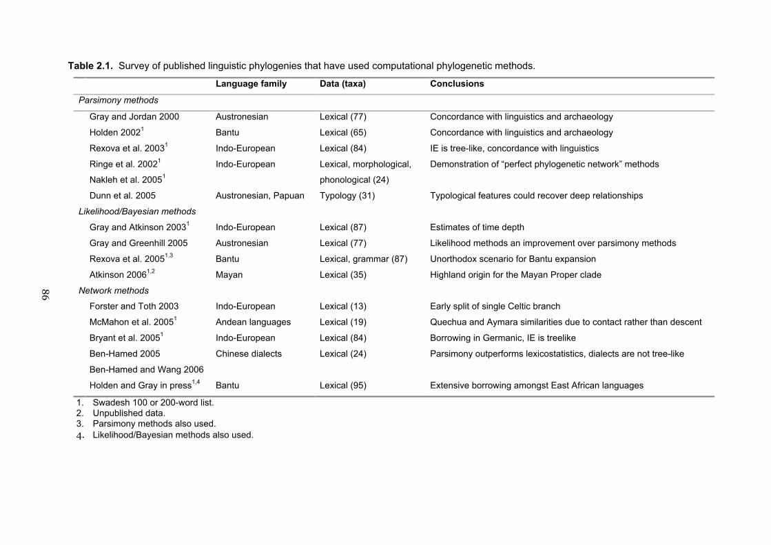
86
Table 2.1. Survey of published linguistic phylogenies that have used computational phylogenetic methods.
Language family Data (taxa) Conclusions
Parsimony methods
Gray and Jordan 2000 Austronesian Lexical (77) Concordance with linguistics and archaeology
Holden 20021 Bantu Lexical (65) Concordance with linguistics and archaeology
Rexova et al. 20031 Indo-European Lexical (84) IE is tree-like, concordance with linguistics
Ringe et al. 20021
Nakleh et al. 20051
Indo-European Lexical, morphological,
phonological (24)
Demonstration of “perfect phylogenetic network” methods
Dunn et al. 2005 Austronesian, Papuan Typology (31) Typological features could recover deep relationships
Likelihood/Bayesian methods
Gray and Atkinson 20031 Indo-European Lexical (87) Estimates of time depth
Gray and Greenhill 2005 Austronesian Lexical (77) Likelihood methods an improvement over parsimony methods
Rexova et al. 20051,3 Bantu Lexical, grammar (87) Unorthodox scenario for Bantu expansion
Atkinson 20061,2 Mayan Lexical (35) Highland origin for the Mayan Proper clade
Network methods
Forster and Toth 2003 Indo-European Lexical (13) Early split of single Celtic branch
McMahon et al. 20051 Andean languages Lexical (19) Quechua and Aymara similarities due to contact rather than descent
Bryant et al. 20051 Indo-European Lexical (84) Borrowing in Germanic, IE is treelike
Ben-Hamed 2005
Ben-Hamed and Wang 2006
Chinese dialects Lexical (24) Parsimony outperforms lexicostatistics, dialects are not tree-like
Holden and Gray in press1,4 Bantu Lexical (95) Extensive borrowing amongst East African languages
1. Swadesh 100 or 200-word list.2. Unpublished data.3. Parsimony methods also used.4. Likelihood/Bayesian methods also used.

87
2.2.7 Algorithms for inferring evolutionary trees
These studies have demonstrated the validity of phylogenetic tree-building using
lexical data with both of the most popular optimality algorithms, maximum
parsimony (MP) and maximum likelihood (ML). Parsimony methods find the shortest
tree: the phylogeny that requires the smallest number of evolutionary changes to
account for the data. In contrast, likelihood methods calculate the likelihood of
observing a particular set of data, given a tree and some explicit model of evolution
(Felsenstein 1981, 2003; Page and Holmes 1999). Parsimony methods have been used
more extensively in the past due to their intuitiveness and ease of implementation, but
ML methods have gained increasing popularity in recent years as computing power,
Bayesian estimation, and more explicit models of evolution have become available
(Pagel 1999b; Huelsenbeck, Ronquist, Neilson, and Bollback 2001). In particular,
likelihood methods outperform parsimony when characters have unequal rates of
evolutionary change (Kuhner and Felsenstein 1994), which is very likely to be the case
in linguistic evolution (Blust 2001). Computer programs implementing phylogenetic
methods allow linguistic phylogenies to be assessed statistically with a variety of
measures: the goodness-of-fit of the data, the amount of support for branches and/or
nodes, comparisons with other trees, and estimates of uncertainty in reconstruction.
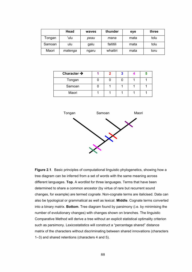
88
Head waves thunder eye three
Tongan 'ulu peau mana mata tolu
Samoan ulu galu faititili mata tolu
Maori matenga ngaru whaitiri mata toru
Character 1 2 3 4 5
Tongan 0 0 0 1 1
Samoan 0 1 1 1 1
Maori 1 1 1 1 1
Figure 2.1. Basic principles of computational linguistic phylogenetics, showing how a
tree diagram can be inferred from a set of words with the same meaning across
different languages. Top. A wordlist for three languages. Terms that have been
determined to share a common ancestor (by virtue of rare but recurrent sound
changes, for example) are termed cognate. Non-cognate terms are italicised. Data can
also be typological or grammatical as well as lexical. Middle. Cognate terms converted
into a binary matrix. Bottom. Tree diagram found by parsimony (i.e. by minimising the
number of evolutionary changes) with changes shown on branches. The linguistic
Comparative Method will derive a tree without an explicit statistical optimality criterion
such as parsimony. Lexicostatistics will construct a “percentage shared” distance
matrix of the characters without discriminating between shared innovations (characters
1–3) and shared retentions (characters 4 and 5).
MaoriTongan Samoan

89
2.2.8 Non-tree methods
Other programs such as NeighborNet (Bryant and Moulton 2004) and SplitsTree
(Dress, Huson, and Moulton 1996) that do not require the data to be represented as a
strict tree can explore and reveal reticulation (borrowing) in linguistic data (Jordan
1999; Ben Hamed 2005; Bryant, Filimon, and Gray 2005; Holden and Gray, in press).
Thus, the common criticism that language (and cultural features in general) do not
evolve in a strictly tree-like fashion can be explored with network models. For
example, in a study of Micronesian and Polynesian languages, the SplitsTree method
revealed borrowing between Ponape (a Micronesian language) and Kapingamarangi (a
Polynesian “Outlier” atoll geographically located in Micronesia) to be responsible for
homoplasy in the language data (Jordan 1999). While network methods can be useful
tools for examining assumptions about the tree-ness of the data and can help identify
sources of reticulation and homoplasy, statistical tests of significance regarding tree-
ness are still being developed. Present comparative methods, however, require a
strictly branching phylogeny to proceed.
2.3 Bayesian methods
2.3.1 Bayesian inference of phylogeny
Comparisons of ML and MP approaches suggest that under many conditions both
methods perform similarly and return concordant topologies, although ML is coming
to be preferred (reviewed in Archibald, Mort, and Crawford 2003; Steel and Penny
2000). Likelihood frameworks have many advantages over parsimony: they use more
information in the data (e.g. branch lengths) and they can incorporate more explicit
and complex models of evolution such as rate heterogeneity (Pagel 1999b). However,
ML methods are hampered by computational inefficiency when dealing with taxa
numbering over about 20. Recently, Bayesian methods have been proposed as a new

90
approach (Rannala and Yang 1996; Larget and Simon 1999; Huelsenbeck et al. 2001).
Bayesian inference is a statistical approach where the model of evolution and the
model parameters are treated as random variables, and the data treated as fixed
observations (Ronquist 2004). In a Bayesian analysis, we update a prior belief
regarding the model and its parameters to a posterior belief once the model and
parameters have been applied to the data (Pagel and Meade 2005).
Applied to the phylogenetic context, these methods simulate a “universe of
trees” which can be sampled to obtain phylogenies in proportion to their likelihood,
and crucially, incorporate the Markov Chain Monte Carlo algorithm, which allows
likelihood methods to be computationally tractable on large data sets (Archibald et al.
2003). These methods differ from other approaches in that they incorporate
uncertainty about the phylogeny by approximating a probability distribution of trees
rather than returning a single, optimal tree. This is especially important in
comparative analyses, where any investigation of correlated evolution may depend on
the particular phylogeny being used, for rarely do we know the true phylogeny without
error (Felsenstein 1988). For example, Ronquist and Liljeblad (2001) investigated the
evolution of gall wasps and their host-plant associations by mapping characters onto a
large sample of trees from a parsimony bootstrap analysis, finding that their results
contradicted many previous hypotheses about the ecological relationships of these
insects.
Phylogenetic uncertainty as a source of error can be addressed using more than
one tree in an analysis, but ad-hoc sets of most-parsimonious trees or random samples
do not provide a statistically principled way to address the problem. Bootstrapping
techniques are resampling-with-replacement methods, and can assess the uncertainty
of an estimate of the phylogeny (Felsenstein 1985, 2003), but they can be
computationally arduous in a likelihood framework. Bayesian methods offer a
workable solution.

91
2.3.2 Markov chain Monte Carlo
Bayesian tree-building methods employ a Markov chain Monte Carlo (MCMC)
algorithm to take a “random walk” through a parameter space (“treespace”) that
approximates a probability distribution. Markov models use a rate matrix Q, which
describes the transition between states of the data (in binary coded language models,
the change from 0 1 and 10) in an infinitely small period of time. To gain the
transition rates for a given data set, the rate matrix is integrated over time as P(t), and
this matrix is used to estimate the transition rates for the observable data (Pagel 1994;
Rohnquist 2004). Each step in the walk, or chain, involves a random modification of a
parameter(s) such as topology or branch length. Periodically, we sample these values
and for each step the posterior probability is calculated. If this is larger than the prior
probability (a value specified by our model), the step is taken. If smaller, then the
action depends on the ratio of the new to the current posteriors. The Markov chain
thus only jumps to a new state as a function of the current state (Pagel and Meade
2005) and does not, like parsimony, hill-climb along a gradient imposed by previous
states. The chain thus visits areas of treespace in proportion to their posterior
probability. Another way to think of the posterior probability of a tree is that it is that
tree’s portion of the overall probability weighted by the prior beliefs (Pagel and Meade
2005). At length, the chain reaches an equilibrium distribution where it is not seeking
an optimally best tree but is sampling better and worse trees into a sample used to
approximate the posterior distribution of all trees.
2.3.3 Support for nodes: Posterior probability distributions
The posterior probabilities (for each node on each possible tree) are a good measure of
nodal support and can be interpreted in a similar manner to the bootstrap in a
parsimony analysis. For example, if 100,000 trees are visited and a group comes out as
monophyletic 78,956 times, then that node has a posterior probability of 0.78956

92
(Lewis 2001). The tree sample can then be summarised to a single phylogeny by some
consensus method that displays the prior probability for particular clades (roughly,
their measure of support), or the tree sample used in further analyses. In a comparison
of MP versus Bayesian likelihood methods on an Austronesian language data set,
Greenhill and Gray (2005) found that Bayesian methods outperformed parsimony in
reconstructing known linguistic subgroups, and concurred more closely with
archaeological models of population dispersal.
2.4 Phylogenetic trees of Austronesian languages
2.4.1 Aims
In this section I describe the language data and tree-building methods used in this
thesis. The results of the phylogenetic reconstructions are described with reference to
previous findings and the linguistic literature.
2.4.2 Austronesian Comparative Dictionary
In previous work with Russell Gray at the University of Auckland, we obtained a
database of Austronesian (AN) languages from Robert Blust at the University of
Hawaii, the Austronesian Comparative Dictionary (ACD) (Blust n.d.). Blust estimated
this to be approximately 25 percent complete. The ACD consisted of 5185 lexical items
across 191 Austronesian languages and was organised so that separate entries consist
of sets of cognate terms (cognacy judgements made by Blust) with the languages in
which they appear. For the purposes of analyses, the presence of a language in a
cognate set was coded as “1” in a languages x words matrix. If a language was not in a
particular cognate set, that language was coded as “0”. Thus the ensuing data matrix
represented presence/absence coding, with cognate words sharing the character state
“1”.
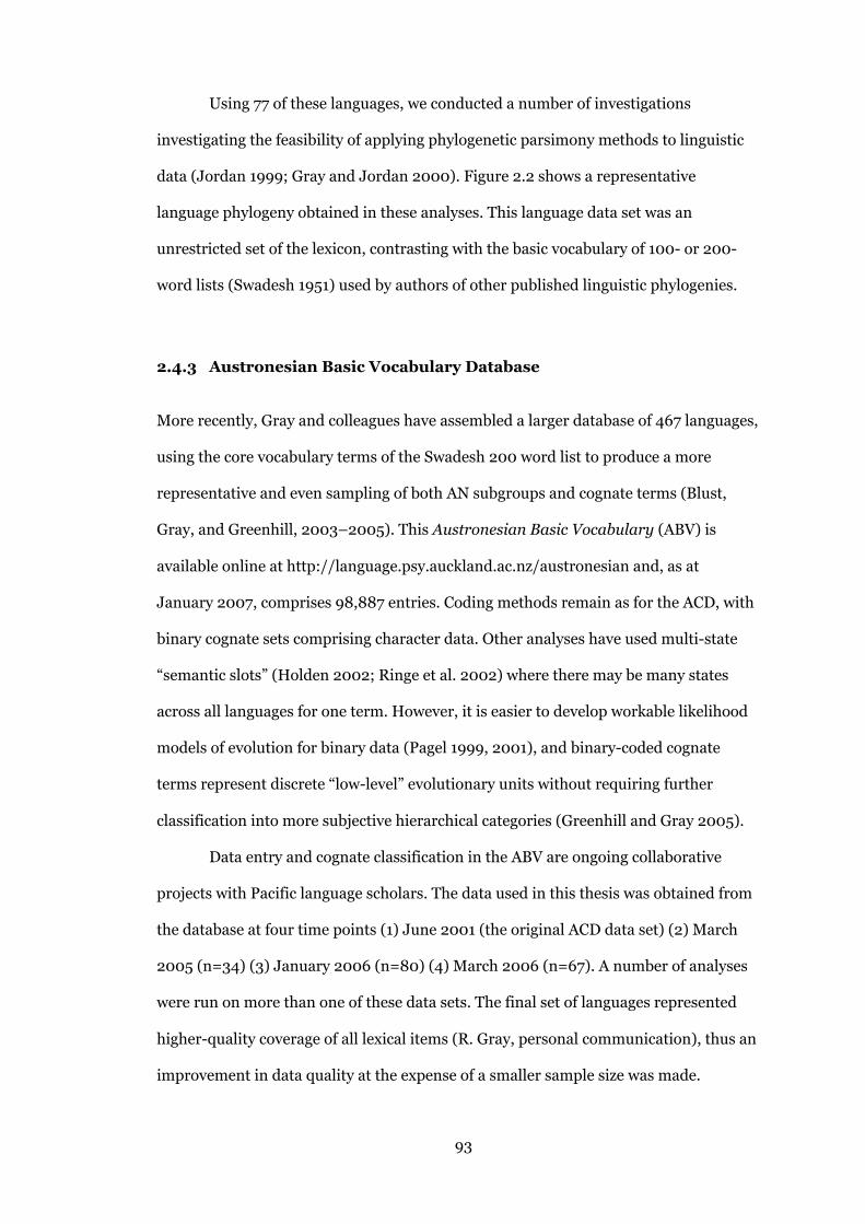
93
Using 77 of these languages, we conducted a number of investigations
investigating the feasibility of applying phylogenetic parsimony methods to linguistic
data (Jordan 1999; Gray and Jordan 2000). Figure 2.2 shows a representative
language phylogeny obtained in these analyses. This language data set was an
unrestricted set of the lexicon, contrasting with the basic vocabulary of 100- or 200-
word lists (Swadesh 1951) used by authors of other published linguistic phylogenies.
2.4.3 Austronesian Basic Vocabulary Database
More recently, Gray and colleagues have assembled a larger database of 467 languages,
using the core vocabulary terms of the Swadesh 200 word list to produce a more
representative and even sampling of both AN subgroups and cognate terms (Blust,
Gray, and Greenhill, 2003–2005). This Austronesian Basic Vocabulary (ABV) is
available online at http://language.psy.auckland.ac.nz/austronesian and, as at
January 2007, comprises 98,887 entries. Coding methods remain as for the ACD, with
binary cognate sets comprising character data. Other analyses have used multi-state
“semantic slots” (Holden 2002; Ringe et al. 2002) where there may be many states
across all languages for one term. However, it is easier to develop workable likelihood
models of evolution for binary data (Pagel 1999, 2001), and binary-coded cognate
terms represent discrete “low-level” evolutionary units without requiring further
classification into more subjective hierarchical categories (Greenhill and Gray 2005).
Data entry and cognate classification in the ABV are ongoing collaborative
projects with Pacific language scholars. The data used in this thesis was obtained from
the database at four time points (1) June 2001 (the original ACD data set) (2) March
2005 (n=34) (3) January 2006 (n=80) (4) March 2006 (n=67). A number of analyses
were run on more than one of these data sets. The final set of languages represented
higher-quality coverage of all lexical items (R. Gray, personal communication), thus an
improvement in data quality at the expense of a smaller sample size was made.

94
Figure 2.2. Shortest tree of 77 Austronesian languages found by parsimony analysis,
from Jordan (1999) and Gray and Jordan (2000). High order subgroups are coloured
as follows: Formosan, Western Malayo-Polynesian, Central Malayo-Polynesian,
South Halmahera-West New Guinea, Oceanic.
Philippines
HawaiianMaoriNiueanRennelleseSamoanTonganPonapeanWoleaiKiribateseMotaFijianLauSaaNggelaArosiManamNumforMussauWuvuluBuliMotuChamorroPalauanRotiYamdenaBuruRembongSikaKamberaManggaraiBugineseMandarWolioMakasareseBareeTaeMalagasyNgaju DayakIbanMalayNiasSimalurDairi Pakpak BatakKaro BatakToba BatakBalineseSasakJavaneseSundaneseOld JavaneseKadazanMukahKayanBario KelabitBolaang MongondowSangirTirurayWestern Bukidnon ManoboMaranaoHiligaynonMansakaKapampanganHanunooBikolTagalogCebuanoBontokKankanayCasiguran DumagatIfugawIlokanoItawisPangasinanIsnegItbayatenAmisPaiwan
Polynesia
Micronesia
Solomons
WMP Outliers
Sulawesi
Indonesia
Borneo
Taiwan
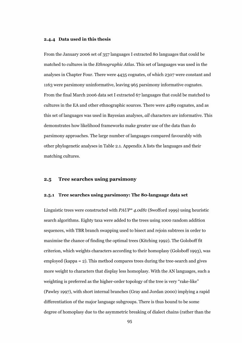
95
2.4.4 Data used in this thesis
From the January 2006 set of 357 languages I extracted 80 languages that could be
matched to cultures in the Ethnographic Atlas. This set of languages was used in the
analyses in Chapter Four. There were 4435 cognates, of which 2307 were constant and
1163 were parsimony uninformative, leaving 965 parsimony informative cognates.
From the final March 2006 data set I extracted 67 languages that could be matched to
cultures in the EA and other ethnographic sources. There were 4289 cognates, and as
this set of languages was used in Bayesian analyses, all characters are informative. This
demonstrates how likelihood frameworks make greater use of the data than do
parsimony approaches. The large number of languages compared favourably with
other phylogenetic analyses in Table 2.1. Appendix A lists the languages and their
matching cultures.
2.5 Tree searches using parsimony
2.5.1 Tree searches using parsimony: The 80-language data set
Linguistic trees were constructed with PAUP* 4.0d81 (Swofford 1999) using heuristic
search algorithms. Eighty taxa were added to the trees using 1000 random addition
sequences, with TBR branch swapping used to bisect and rejoin subtrees in order to
maximise the chance of finding the optimal trees (Kitching 1992). The Goloboff fit
criterion, which weights characters according to their homoplasy (Goloboff 1993), was
employed (kappa = 2). This method compares trees during the tree-search and gives
more weight to characters that display less homoplasy. With the AN languages, such a
weighting is preferred as the higher-order topology of the tree is very “rake-like”
(Pawley 1997), with short internal branches (Gray and Jordan 2000) implying a rapid
differentiation of the major language subgroups. There is thus bound to be some
degree of homoplasy due to the asymmetric breaking of dialect chains (rather than the
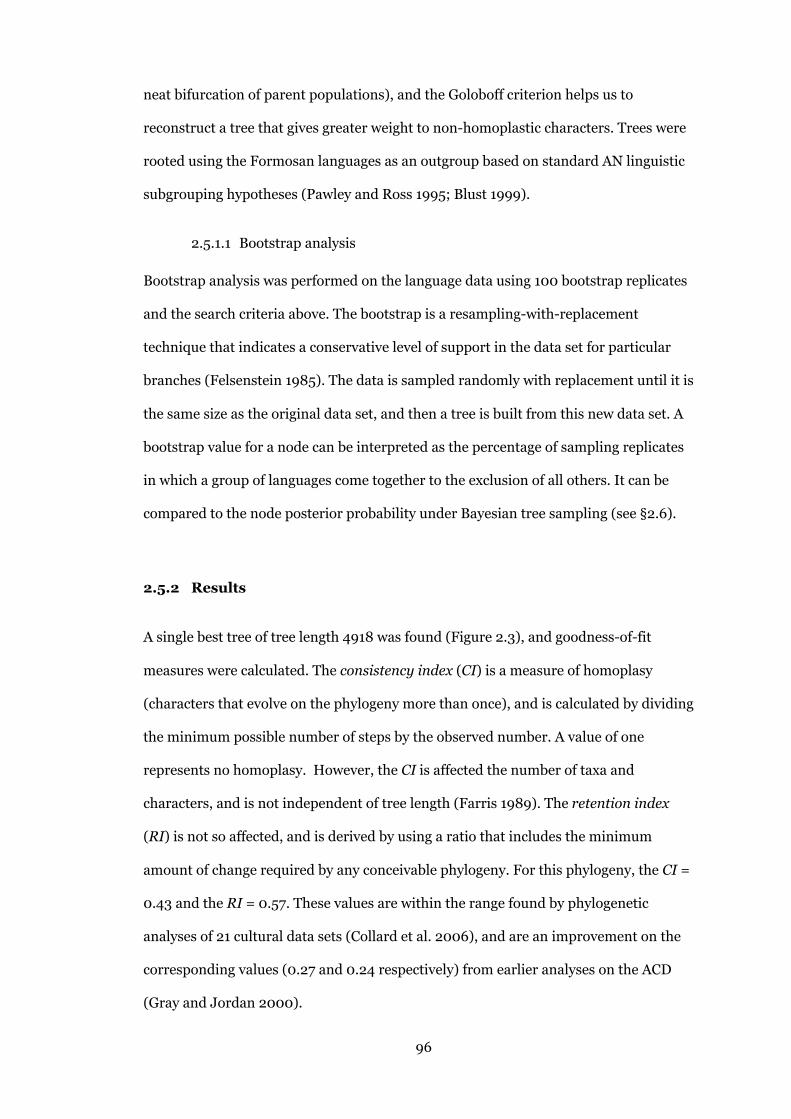
96
neat bifurcation of parent populations), and the Goloboff criterion helps us to
reconstruct a tree that gives greater weight to non-homoplastic characters. Trees were
rooted using the Formosan languages as an outgroup based on standard AN linguistic
subgrouping hypotheses (Pawley and Ross 1995; Blust 1999).
2.5.1.1 Bootstrap analysis
Bootstrap analysis was performed on the language data using 100 bootstrap replicates
and the search criteria above. The bootstrap is a resampling-with-replacement
technique that indicates a conservative level of support in the data set for particular
branches (Felsenstein 1985). The data is sampled randomly with replacement until it is
the same size as the original data set, and then a tree is built from this new data set. A
bootstrap value for a node can be interpreted as the percentage of sampling replicates
in which a group of languages come together to the exclusion of all others. It can be
compared to the node posterior probability under Bayesian tree sampling (see §2.6).
2.5.2 Results
A single best tree of tree length 4918 was found (Figure 2.3), and goodness-of-fit
measures were calculated. The consistency index (CI) is a measure of homoplasy
(characters that evolve on the phylogeny more than once), and is calculated by dividing
the minimum possible number of steps by the observed number. A value of one
represents no homoplasy. However, the CI is affected the number of taxa and
characters, and is not independent of tree length (Farris 1989). The retention index
(RI) is not so affected, and is derived by using a ratio that includes the minimum
amount of change required by any conceivable phylogeny. For this phylogeny, the CI =
0.43 and the RI = 0.57. These values are within the range found by phylogenetic
analyses of 21 cultural data sets (Collard et al. 2006), and are an improvement on the
corresponding values (0.27 and 0.24 respectively) from earlier analyses on the ACD
(Gray and Jordan 2000).

97
Figure 2.3. Maximum parsimony tree of 80 Austronesian languages. Numbers above
branches are bootstrap values, indicating the percentage of times that a node was
recovered in the 100 bootstrap replicates; these are only reported for values > 50.
Language subgroups are colour-coded to reflect standard AN subgroups (top-left).

98
2.5.3 Tree topology
The tree corresponds to many of the major subgroups of the Austronesian language
family (see top-left Figure 2.3 for traditional linguistic classification of AN). The
Formosan languages are at the base of the tree. Neither the WMP or CMP languages
fall out as an exclusive clade derived from a single common ancestor, that is, they do
not display monophyly. This may reflect current thought that there is no strong
evidence for either WMP or CMP as exclusive subgroups; they should be thought of as
linkages (Blust in press) or as several primary branches of Malayo-Polynesian (Gordon
2005). The Sundic languages fall inside a group with languages from Sulawesi. This
group also contains the Philippine languages, except Bontok, which groups more
basally with Yami (spoken on Botel Tobago between the Philippines and Taiwan). The
CMP languages constitute two separate branches whose members correspond to low-
level subgrouping hypotheses (Tryon 1995). This is true of most of these WMP/CMP
languages, except Malagasy, which should fall in with Iban.
An anomalous grouping of Yapese, a Micronesian language of contentious
placement, the lone SH-WNG representative Waropen, and Tannese and Lifu is most
likely a result of “missing cognacy” for these languages (S. Greenhill, personal
communication). Thus, parsimony is able to group them within the Oceanic group but
relegates them to the base, as the program will assume that their lack of cognacy with
other languages indicates early branching.
Within the Oceanic languages several subgroups are recovered. The
Micronesian languages form a monophyletic group, as do Central Pacific and
Polynesian. The Polynesian languages contain an Eastern Polynesian clade (Marck
1999). The Southeast Solomon languages, along with Mota (Vanuatu) form a group.
The remaining Western Oceanic and Admiralties languages are variably resolved, in
accordance with the well-known “rake-like” structure of those parts of the Oceanic
language family. In this situation, the bifurcating tree model appears least applicable
due to a rapidly dispersing and unevenly-breaking dialect network (Ross 1997; Pawley

99
1997), and accordingly, the hierarchical arrangement of these languages is poorly
supported by the bootstrap values. Overall, this tree contains many attested subgroups
of Austronesian, recovers relationships of sister-taxa well, and is comparable to
standard hypotheses in its outline. This phylogeny was used in Chapter Four as a
model of population history.
A single phylogeny, however, cannot capture the degree of uncertainty that
must necessarily be present in the historical relationships of human groups. The
following section described and presents the results of Bayesian phylogenetic analyses
that address this problem.
2.6 Tree searches using Bayesian methods
2.6.1 Bayesian estimation of phylogeny
A variety of computer programs for ML and/or Bayesian estimation of phylogeny have
become available recently such as MrBayes (Huelsenbeck and Ronquist 2001) and
BAMBE (Simon and Larget 2000). I used BayesPhylogenies (Pagel and Meade 2004;
UNIX binary available at http://www.evolution.rdg.ac.uk/BayesPhy.html) to obtain a
posterior probability distribution of trees under this method because the outputs were
directly related to the comparative methods BayesMultiState (Pagel, Meade, and
Barker 2005) and Discrete (Pagel 1994) that I used in later chapters. In addition,
BayesPhylogenies contains models of evolution that have been developed for use on
language data (M. Pagel, personal communication).
I used the Bayesian MCMC method in BayesPhylogenies to estimate a
posterior probability distribution of trees. This is not a set of optimally likely trees, but
rather a set of trees where topologies are represented in proportion to their
likelihood—that is, they contain some low, some high, and some intermediate values of
likelihood and the set is thus a distribution with likelihood on the x axis and frequency
on the y.

100
2.6.2 Analyses
2.6.2.1 Initial Bayesian analyses
The 80 language data set was initially used to build language trees under various
combinations of model parameters and outgroup designations (not shown). The great
majority of the trees in the outcome of these analyses contained subgroups of
languages in non-standard placements, such as the Polynesian languages at the base of
the tree. In addition, single languages would “float” about the tree, showing no stability
of placement. The improvement in data quality in the 67 language data set was
demonstrated in greater stability of the major subgroups. This led to the decision to
use the smaller sample size of 67 languages.
2.6.2.2 Models of word evolution and the choice of priors
The MCMC method can implement one of two different statistical models of word
evolution for discrete binary characters (BayesPhylogenies software,
http://www.evolution.rdg.ac.uk). These are based on those models used in papers
describing the software (Pagel et al. 2004). M1P is a one-parameter model in which the
rates of gain and loss of words are presumed to be equal. M2P is a two-parameter
model where rates of gain and loss can be unequal, but can be computationally time-
consuming with large data sets; therefore, M1P models were used preferentially. Word
meanings were allowed to evolve at different rates drawn from a gamma distribution
with four rate categories (Yang 1994). Base frequencies of the character states were
estimated from the data.
The prior. In a Bayesian analysis, we calculate the posterior probability of the
data given a tree and a model of evolution, but we require a prior belief about the
probability of the tree and model parameters in advance. The choice of prior is a
controversial aspect of Bayesian phylogenetic analysis as it can be regarded as
subjective (Alfaro and Holder 2006). By using a uniform prior, all parameters and
topologies are considered equally likely, introducing no further assumptions about the
101
model of word evolution. The program routine is thus free to propose any combination
of (for example) branch lengths and topologies on each step. Alternatively, we can
specify a more informative prior if we have background information (Ronquist 2004),
or we can use a non-uniform prior such as a probability distribution with a specified
mean. Uniform priors were used in the generation of Bayesian tree samples1, as they
are effective when the phylogenetic signal in the data is strong (Pagel et al 2004).
2.6.2.3 Outgroup rooting
Old Chinese (a non-Austronesian language included in the ABV for comparative
purposes) was initially used to root the tree, although this language could not be tied to
a particular ethnographic source (Sagart 1993). Preliminary tree searches revealed that
this choice of outgroup found trees in which the Formosan (Taiwanese) languages fell
out basally, in accordance with standard Austronesian linguistic theory (Pawley and
Ross 1993; Blust 1999). In two out of three tree searches the Formosan languages
formed a monophyletic group and in the other Atayal and Bunun formed the first,
post-Old Chinese branch. Sagart (2004) has recently suggested that Atayal may be the
earliest branching of the Formosan languages in this data set, based on an hypothesis
that early AN expansion took place counter-clockwise in a circle around Taiwan,
starting from the north-east (2004:437). Tree searches where Atayal was used as a
single language to root the tree produced phylogenies with peculiar arrangements of
the Polynesian and WMP languages. As the analyses with Old Chinese had
demonstrated their placement at the base of the tree, I used the five Formosan
languages in the sample (Atayal, Ami, Bunun, Paiwan, and Puyuma) as outgroup taxa
in all subsequent analyses.
1 In comparative analyses (Chapter Three) where signal is weaker due to fewer data points, an exponentially distributedprior was used on the assumption that very high rates of cultural change were not as likely as lower or moderate rates.This was a conservative assumption and did not affect the ancestral state reconstructions except to reduce uncertaintyby small (<.10) amounts.

102
2.6.3 Results
2.6.3.1 MCMC sample
The Markov chain, the states of which are different phylogenies, started from a
random tree and was sampled every 1000 trees. Four separate chains were run to
ensure that the analyses converged to the same region of the space of possible trees.
Chains were run for between 1 x 10⁶ and 10 x 106 iterations. Each run included a “burn-
in” period before the log-likelihood values converged on a fluctuating value
(stationarity). Trees from the burn-in period were discarded from the sample, and the
final posterior probability distribution (PPD) consisted of 1000 trees sampled every
2000 iterations from one of the post-convergence chains. The PPD is a distribution
containing not only topologies of trees and their likelihoods, but is also a distribution
of branch lengths and the other parameters, such as transition rates, estimated by the
model of word evolution (Pagel and Meade 2005).
2.6.3.2 Autocorrelation
The degree of autocorrelation between successive trees in the probability sample was
calculated in order to test for independence. When the chain is still in the convergence
period, successive topologies should be increasing overall in their likelihood. Post-
convergence trees and their likelihoods should wander about the likelihood surface
without apparent pattern, and autocorrelation should thus be very close to zero. By
plotting likelihoods against their iteration, autocorrelation can be calculated. Here,
r = 0.00037. Figure 2.4 shows the convergence of the Markov chain from the random
starting point towards equilibrium. The inset shows how the Markov chain wanders
around the equilibrium point after convergence. The posterior probability distribution
of the log-likelihoods that were sampled post-convergence is shown in Figure 2.5. The
distribution is approximately normal with a mean of -51859.5 ± 23.82.

103
Figure 2.4. Convergence of the Markov chain through 3,000,000 iterations. The chain
takes some time to reach stationarity, with the likelihood gradually increasing through
the first million iterations. The inset shows a portion of the chain around 2.5 million
iterations, demonstrating how the likelihood wanders up and down around a central
tendency but does not show a directional trend.

104
Figure 2.5. Posterior probability distribution of log-likelihoods in the 1000 phylogenetic
trees sampled from the converged Markov chain. The distribution is effectively normal
(kurtosis = -1.2, skewness = 0.000), with a mean of -51859.5 ± 5.52. The majority of
the sample features trees of intermediate likelihood, with only a few very good or very
poor likelihoods.

105
2.6.4 Bayesian phylogeny
The consensus linguistic phylogeny of 67 AN languages is shown in Figure 2.6.
Consensus trees are not the “best” tree or even necessarily an actual tree present in the
sample but rather display a summary of the nodes frequently found in the sample.
Figure 2.7 shows six phylogenies drawn at random from the sample, to illustrate the
range of variation within and to stress that the sample is a distribution. In Figure 2.6
each node is labelled with the posterior probability of that node—the probability that
the node is true, given the model of evolution—and reflects the number of times a node
appears in the sample. The node’s posterior probability is a measure of stability within
the sample, not of confidence in general (Pagel and Meade 2005). That some of the
nodes have a low posterior probability reflect the importance of using statistical
approaches that take uncertainty about the phylogeny into account.

106
Figure 2.6. Consensus linguistic tree of the Bayesian 1000-tree sample. Full descriptionfollows on the next page.

107
Figure 2.6. (on the previous page). Consensus linguistic tree of the 1,000-tree sample,
showing clades present in over 50% of the sample as well as those that do not conflict
with the majority. Figures over branches correspond to the posterior probabilities of the
nodes. A value of 100 indicates that a node appeared in every tree in the sample.
Black circles indicate those nodes with a posterior probability distribution >0.70, a
threshold for confidence in the existence of that node (Pagel 1999b), while white
circles indicate a PPD <0.70. Nodes denoting language subgroups/proto-language
stages are as follows: PAN Proto Austronesian, PMP Proto Malayo-Polynesian, PCE
Proto Central-Eastern Malayo-Polynesian, POC Proto Oceanic, PCP Proto Central
Pacific, CMP, Central Malayo-Polynesian, Mic Micronesian, Pol Polynesian, Form
Formosan. Other nodes are labelled as: Phil Philippines/Sulawesi, Indo Indonesia
OCW Oceanic-West.
Figure 2.7. (on the following page). Six trees drawn at random from the Bayesian
sample of 1,000 trees in order to give an indication of the variation contained therein.
Arrows indicate differences from the consensus tree in Figure 2.6, described for each
tree as follows: (1) the clade of Ambon, Kei, and Tanimbarese is basal to the CMP
group; (2) Micronesian and Polynesian are sister-clades; (3) the clade of Nias,
Malagasy, and Melanau falls outside the Indonesian group; (4) Nias is basal to the
Indonesian grouping; (5) Ponape groups with the western Micronesian languages (6)
three different most-recent sister-taxa for Lakalai, Marquesan, and Hanunoo.
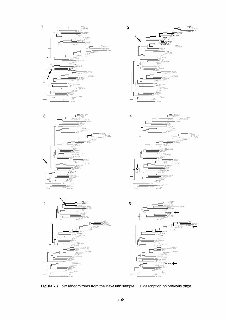
108
Figure 2.7. Six random trees from the Bayesian sample. Full description on previous page.

109
2.6.5 Topology
The consensus tree recovers all the major subgroups of the Austronesian language
family (highlighted in coloured groups). The Formosan languages consistently divide
into two groups that do not reflect any standard linguistic hypothesis, as Atayal groups
with Ami and Bunun, rather than forming a basal branch (Blust 1999; Sagart 2004).
This may, however, be an artefact of the artificial monophyly imposed by the outgroup
method.
As in the parsimony analysis, the WMP languages do not fall out as a
monophyletic group. Rather, they group into a well-supported clade (mean PPD = 67)
of Philippine languages and a less well-supported group (mean PPD = 47) of
Indonesian languages from Sumatra, Borneo, and Java. The Philippine languages
(including Yami) fall out as monophyletic, a hypothesis supported by the majority of
Austronesian linguists (Zorc 1986; Blust 1991) Within the second group, the Sundic
languages including Malay fall out as an exclusive clade (mean PPD = 79), and the
Sulawesi languages (Macassarese, Toradja) also come together consistently. The
placement of Malagasy next to Melanau, spoken on Borneo, makes good sense, as
Proto Malagasy is thought to have originated in Borneo c. 1200 BP (Dahl 1991). Nias,
off the southeast coast of Sumatra, may have been excluded from the “linguistic
levelling” that took place in many WMP languages through the last millennium
(Nothofer 1990, 1991). This homogenisation may have been due to widespread trading
networks and the influence of Indian, then Islamic influences (Bellwood 1997), as well
as the growth of Malay and Javanese as a lingua franca. Thus, populations that were
outside the central Indonesian sphere of interaction may group together simply due to
shared retentions of earlier linguistic forms rather than reflect the budding off of
daughter populations.
A Central-Eastern Malayo-Polynesian node is strong (mean PPD = 99),
splitting into equally strong CMP (there are no SH-WNG languages in this sample) and
Oceanic groups. Internal resolution in this group is fair at more recent levels, but only

110
the Bima-Sumbanese clade (Kodi, Sumbanese, Manggarai) has good support. This is
interesting, as evidence for the Bima-Sumba group has been called elusive by Blust
(1993b).
The Oceanic group divides into two branches, one representing the Central
Pacific group (Geraghty 1983) of Fiji, Rotuma, and the Polynesian languages and the
other consisting of a strong clade of Western Oceanic (excluding Lakalai), Micronesian
(whose internal relationships are not well resolved, though the clade itself has strong
support) and uncertain arrangements of the other languages from Vanuatu, the
Solomons, and the Admiralties. While the Eastern Polynesian subgroup appears as a
clade, the internal structure of the Polynesian languages is counter to current
hypotheses (Pawley 1996) that group Tongic languages (Tonga and Niue) exclusive of
and basal to the rest, but supports the paraphyly of the other Nuclear (but not Eastern)
Polynesian languages as Marck (1999) suggested. It may be that despite the long-
standing cliché of the “island laboratory” model of cultural evolution in Polynesia,
implying a bifurcating tree model and isolated populations, there is considerable
evidence for language reticulation and contact amongst these populations. Preliminary
analyses using network models show this to be true of both Polynesia and Micronesia
(Jordan 1999; S. Greenhill, personal communication).
Overall the tree has short internal branch lengths, especially at the base of the
tree, and longer terminal branches. This could imply that (i) much of the language
evolution has taken place in terminal taxa, and relatedly (ii) that the language data
contains many unique characters, (iii) that homoplasy and reticulation through, for
example, the breaking of dialect chains, has led to conflicting signals in the data, or (iv)
that dispersion of the languages was rapid enough for cumulative change along the
deeper branches to be fairly minor. Most likely a combination of these factors will
account for this topology. Factors (i) and (ii) are certainly an influence, as terminal
branches are long, and approximately 10 percent of the characters are unique to a
single language, while the presence of dialect-chain breaking in Oceanic languages is

111
well-attested (e.g. Geraghty 1983; Ross 1997). Recent Bayesian analyses with the entire
ABV data set (350+ languages) support the notion that rapid dispersion is a strong
feature of these languages (R. Gray, personal communication).
2.6.6 Comparison with other results
Compared to the parsimony tree of 80 AN languages (§2.5), the consensus phylogeny
of the 1000 tree sample is superior in two respects. Firstly, this Bayesian tree is more
resolved, especially at deeper nodes, allowing us to have more confidence in the
historical relationships indicated by the tree. The bootstrap and posterior probabilities
of nodes are superficially comparable as measures of support, although they are not
mathematically equivalent (Felsenstein 2003). Where comparable across trees,
Bayesian posterior probabilities are virtually always higher than the corresponding
bootstrap, although bootstraps are known to be conservative (Alfaro et al. 2003;
Doaudy et al. 2003). For example, the parsimony analysis returned a bootstrap value
of 76 for the Eastern Polynesian languages, while support was at 100 percent for the
Bayesian posterior probabilities. Secondly, the phylogeny produced by this Bayesian
analysis conforms more to standard linguistic hypotheses than does the parsimony
tree.
Although the sample of languages differs significantly, the Bayesian analysis of
the 77 ACD languages by Greenhill and Gray (2005) included most of the main
subgroups of AN included here. Like here, they found high posterior probabilities for a
Philippine subgroup, but no evidence for a monophyletic WMP group. They also
recovered a well-supported Sundic group and probabilities approaching 100 on the
Micronesian and Polynesian subgroups. With respect to topologies, Greenhill and
Gray’s trees show a similar pattern of some very short internodes and some longer
ones, with intriguing hints that this may correspond to expansions and pauses in
population dispersals (Greenhill 2004).

112
2.7 Conclusions
Both parsimony and Bayesian likelihood methods returned phylogenies that provide
useful models of population history. They conform to standard subgrouping
hypotheses of Austronesian languages, and display statistical properties indicating
they are robust phylogenies. These trees are used in the following chapters. The
parsimony tree provides phylogenetic distances and phylogenetic nearest neighbours
for the analyses in Chapter Four. The Bayesian sample of 1000 trees has been used in
all comparative analyses of residence and descent that use BayesMultiState (Chapters
Five and Six), and the consensus phylogeny of the Bayesian sample has been used in
Chapter Seven with the program Continuous to investigate the relationship between
language change and population size.

113
CHAPTER THREE
THE COMPARATIVE METHOD IN ANTHROPOLOGY
3.1 Summary
Comparative methods for phylogenetic tests are introduced. Parsimony and likelihood
methods are contrasted. Likelihood models allow uncertainty to be incorporated into
comparative analyses. A likelihood ratio test can choose between an independent and
dependent (co-evolutionary) model for discrete traits evolving on a phylogeny. The
Bayesian approach to comparative analysis using the Bayes Factor as a test statistic is
described in detail. Reverse-jump MCMC, a new method for estimating the
appropriate model of trait evolution, is described. Bayesian frameworks are powerful
tools for the investigation of cultural trait evolution, and are exploited in subsequent
chapters.

114
3.2 Introduction
3.2.1 The comparative method
Lions and tigers and bears are separate species, but they do not provide us with three
separate instances of the evolution of meat-eating. They are all members of the
mammalian order Carnivora, and, because the branching process of evolution means
that species share common ancestors, we cannot therefore treat them as independent
outcomes in statistical analyses. If we incorporate the phylogenetic pattern of descent
amongst a group of species into an analysis, we will count only those branches (rather
than species) on which evolution has taken place. Methods that control for historical
relationships are called phylogenetic comparative methods. Comparative methods test
for regular associations between variables across a number of hierarchically related
taxa (e.g. species, populations, cultures), and such correlations are generally
interpreted as the best evidence for co-evolution or adaptation (Clutton-Brock and
Harvey 1977; Ridley 1983; Harvey and Pagel 1991). While tests vary, comparative
methods generally proceed by plotting character states (for example, colouration and
environment) on the branches of a phylogeny. Some optimality criterion, often
parsimony or likelihood, is then used to reconstruct ancestral states, identify
independent instances of evolutionary change, and from these, evaluate the statistical
evidence for co-evolution of the characters.
Chapter One outlined Galton’s Problem in anthropology, that is, the analogous
need to control for the historical non-independence of cultures when conducting cross-
cultural tests. Comparative methods from evolutionary biology address this need. With
respect to cultural evolution, by using a linguistic phylogeny as a proxy for population
history we are able to place known character states of the “ethnographic present” on
the phylogeny and reconstruct cultural traits for putative parent populations. Thus, if
we have a hypothesis of the historical relationships between a group of cultures (a tree
phylogeny), and information about the variation in cultural traits amongst them, then
115
we are able to make quantitative inferences about the possible states of these cultural
traits in the past.
Data for use in comparative analyses can be discrete or continuous. Discrete
data can be binary, indicating the presence or absence of a variable. For example,
Holden and Mace (2003) coded cattle-keeping and matriliny as present or absent in
their co-evolutionary analysis of descent and pastoralism in Bantu cultures. Discrete
data may also be multi-state, that is, exist in more than two categories but not have an
ordinal relationship. For example, human marriage systems might be classified as
polygynous, monogamous, and polyandrous. Continuous data are often used in
evolutionary biology and are some measurable trait of an organism such as body mass
or population sex ratio. In cross-cultural tests, continuous variables include traits such
as dependence on horticulture for subsistence (expressed as a percentage) or the
sexual division of labour (Murdock 1967). The type of data may affect what
comparative method the investigator uses. Below I discuss different types of
comparative methods and their advantages and disadvantages.
3.3 Parsimony-based methods
3.3.1 Characteristics of parsimony-based comparative methods
Parsimony methods of ancestral state reconstruction minimize the number of
evolutionary changes on the phylogeny required to explain the observed character
distribution at the tips. For instance, if two sister taxa share a trait, then the ancestor
of those two is assumed to have the trait, rather than positing two separate instances of
character evolution. Comparative methods employing parsimony differ according to
whether variables are discrete or continuous. For discrete data, parsimony methods
test whether changes in a binary character are randomly distributed over the branches
of the phylogeny (Ridley 1983; Maddison 1990). MacClade (Maddison and Maddison
1992) and Mesquite (Maddison and Maddison 2006) implement versions of these
116
concentrated-changes tests. For continuous data, or a combination, Felsenstein’s
(1985) method of independent contrasts is widely used, and is commonly implemented
in the program CAIC (Purvis and Rambaut 1995). By virtue of sharing a common
ancestor, the differences in traits between sister-taxa are independent of the
differences between other sister-taxa pairs on a phylogeny; the same logic holds true
for all adjacent nodes across the tree. These phylogenetically controlled independent
contrasts can then be used in standard correlations. Other methods exist, including
autocorrelation and generalised least-squares (GLS) (Cheverud, Dow, and Leutenegger
1985; Martins 1995; reviewed in Rohlf 2001).
3.3.1.1 Shortcomings of parsimony
While intuitively easy to understand, there are some problems with parsimony-based
comparative methods. Most do not use branch length information and thus if traits
evolve at different rates over the tree they may under- or overestimate the number of
evolutionary changes. As well, some of these methods do not perform well under
conditions of rapid evolutionary change (Cunningham 1998). All assume a
neutral/drift model of trait evolution (Steel and Penny 2000), and none are able to
detect the order of character changes (i.e. the direction of causality in adaptive
change). Likelihood-based and Bayesian comparative methods offer a useful
alternative, the key points of which are summarised in Table 3.1.

117
Table 3.1 Comparison of parsimony and likelihood-based comparative methods.
Parsimony Approaches Likelihood/Bayesian
Approaches
Ancestral state
reconstruction
Single value assigned to each
character at internal nodes
Probability distribution of character
states at internal nodes
Phylogenetic
uncertainty
Most treat phylogeny as known
without error
Some methods incorporate
uncertainty by using a tree sample
Character-mapping
uncertainty
Ancestral states treated as
known
May underestimate amounts of
change
Ancestral states treated as
probabilistic states
Useful when trait evolution may be
rapid
Branch length Information generally not
incorporated into model
Information incorporated; used to
calculate rates of character
transition
Models of evolution Neutral drift (“Brownian motion”) Stochastic; Bayesian methods
allow for the specification of a prior
model
Gains and losses,
rates of evolution
All types of change treated as
equally likely
Transition-rate parameters
calculated for each type of change,
rates of evolution can be
calculated
Order of changes Difficult to detect Possible to detect
Incorporation of prior
information
None Defining characteristic of Bayesian
methods
Computational
abilities
Fast Can be slow, Bayesian estimates
improve speed
118
3.4 Likelihood comparative methods
3.4.1 Characteristics of likelihood-based comparative methods
Maximum-likelihood phylogenetic methods ask about the probability of the observed
data, given a phylogeny and some specified model of evolution. These methods offer
several advantages over parsimony methods (Table 3.1), most notably that they
incorporate uncertainty about ancestral character states and rates of evolution by
estimating a model of probability distributions and rate parameters. Few comparative
methods use likelihood frameworks, but those that do include certain modules in
Mesquite (Maddison and Maddison 2006), SIMMAP (Bollback 2006) and the methods
by Pagel and colleagues (Pagel 1994, 1997, 1999a, 1999b; Pagel et al. 2004).
3.4.1.1 Pagel’s method
Pagel (1994) described a likelihood ratio test (implemented in the program Discrete
and in a Bayesian framework in BayesMultiState) that allows testing for correlated
evolution by comparing two models; the independent model, where two characters
evolve independently, and the dependent model, where characters evolve together
(Pagel 1994; Pagel 1999b). In the course of this analysis, the programs also reconstruct
the probability of ancestral states at each node in the tree. Transition-rate parameters
(the probability of change from 01 and 10) are estimated for each model, using a
continuous time-varying Markov model (Figure 3.1). The likelihood of the data given
the tree is calculated using the logic that if the two variables change independently, the
joint probability of change equals the product of the separate probabilities of change.
The likelihood of assigning the state of a variable to the terminal branches of the tree
(the “tips”—our taxa of interest) is given by the product over all of the branches of the
tree. Simply put, this method searches for the transition-rate parameters in two
models—independent and dependent—that make the observed data most likely, and
compares the obtained likelihoods.

119
Figure 3.1. The two models estimated in Pagel’s likelihood/Bayesian methods (1994,
1999, 2004), and their transition-rate parameters.
X Y
α1
β1
X Y
α2
β2
Trait A Trait B
Y,X
Y,Y
X,Y
X,X
q12
q21
q24
q13
q42
q34
q43q31
Trait A
Trait B
Independent (Null) Model.Traits may take two states, X and Y. On this model, Trait A evolves independently of the state ofTrait B on each branch of the tree. Four transition-rate parameters (α1, α2, β1, β2) are estimatedthat account for the evolutionary change in the data, given the phylogenetic model.
Dependent (Correlated) Model.Traits may take two states, X and Y. On this model, the state of Trait A is dependent on the stateof Trait B in each branch of the tree, effectively creating four ‘states’. Note that because changeis dependent, moving from XX (state 1) to YY (state 4) requires two steps. Eight parameters(q12, q21, q13, q31, q24, q42, q43, q34) must be estimated by the model to account for the data.

120
Once we obtain the likelihood scores for the two models we can compare the likelihood
of each model. This assesses the goodness of fit by calculating the likelihood ratio:
LR = -2 loge [lh(I)/lh(D)] [Eq. 1]
Where lh(I) is the likelihood of the independent model and lh(D) is the likelihood of
the dependent model. By simulating a null distribution of LR scores, we can use the
chi-square distribution (with degrees of freedom equivalent to the difference in model
parameters) to compare if our obtained LR for the independent and dependent model
is significant. If it is, and the dependent model fits significantly better, this method
provides us with evidence for correlated evolution.
Phylogenies impose a correlation on characters, even if they evolve
independently (Lewis 2001). The model implemented by Pagel’s methods test if the
correlation is above the one that is imposed phylogenetically. The null model of
independent evolution is a constrained version of the general model, as the correlation
is constrained to zero, thus, the dependent model will fit better than the independent if
the true correlation between the characters is not equal to zero.
3.4.2 Bayesian comparative methods
Bayesian comparative methods incorporate the likelihood-based estimation of
ancestral states and correlated evolution (i.e. by estimating rate parameters that
explain the observed data) with a Bayesian-derived tree sample to represent
phylogenetic uncertainty. Many methods deal with this uncertainty by using the “best”
tree by some optimality criterion, or a consensus tree derived from a set of “best” trees,
yet neither can be presumed to be the true tree. Bayesian approaches to estimating
uncertainty about the phylogeny were described in Chapter Two. Similarly, many
comparative methods work by assigning a single value of a character state to each
node, producing a source of error called mapping uncertainty (Frumhoff and Reeve

121
1994; Ronquist 2004). Bayesian comparative methods address both these source of
uncertainty by implementing a Markov model that estimates rate transitions of
character states in a similar fashion to the rate matrices described for word evolution
in §2.6.2.1, then integrates these rates, and other parameters in the model, over a
posterior probability distribution of trees. The probability of a particular character
state at a particular node, or a combination of states when testing for co-evolution, is
thus weighted by the likelihood of that node appearing in the data set.
3.4.2.1 BayesMultiState
Lutzoni, Pagel, and Reeb (2001) used Discrete to investigate the ancestral states of
lichen-forming Ascomyta fungi, estimating character states at each node over a
Bayesian sample of trees and generating likelihood plots of character-state likelihood x
node likelihood. These plots were then used in conjunction with the consensus
phylogeny to interpret the symbiotic evolution of lichen and fungi. More recently,
Pagel et al. (2004) described an integrated procedure for the Bayesian estimation of
ancestral states at internal nodes, released as the program BayesMultiState. Using the
posterior probability distribution of trees rather than a single phylogeny, ancestral
states are estimated over the entire tree sample. Here, the likelihood of a state at a
particular node is further moderated by the likelihood of that node existing in the tree
sample, taking a statistically principled approach to uncertainty about both phylogeny
and mapping (character-state) reconstruction.
An example describes this approach. We may wish to calculate the ancestral
state of marriage patterns, for example the presence of polygyny, in Eastern Polynesian
and Philippine cultures. We have a Bayesian sample of language phylogenies, as
described in Chapter Two. In this sample, the posterior probability distributions are
0.98 for the Eastern Polynesian node and 0.67 for the Philippine node. This represents
our phylogenetic uncertainty. The comparative method (described below) estimates
the PPD for polygyny in the two groups of cultures, and returns 0.75 for Eastern
Polynesia, and 0.99 for the Philippine group. This represents our mapping uncertainty.
122
We then multiply the uncertainties together to ask the question: “What is the
likelihood of the ancestral state being polygyny, given uncertainty about character-
state reconstruction and uncertainty about the phylogeny?” In this example, although
the character-state estimation for the Philippine cultures is very certain, the Philippine
node only exists on two-thirds of the trees in the sample, reducing the ancestral state
estimation to 0.66. However, the Eastern Polynesian group is very robust, so the
ancestral state estimation remains high, at 0.74. By identifying the sources of
uncertainty in this way, we can make more realistic inferences about evolutionary
processes.
Correlated evolution can be tested, as the BayesMultiState program
implements a Bayesian version of the Discrete test of independent and dependent
models as described above (Pagel and Meade 2006), and also implements the
Continuous algorithm for continuous data (Pagel 1997) into the software. In this
thesis, all comparative analyses of ancestral state reconstruction, evolutionary rates,
and co-evolutionary hypotheses were tested, where appropriate, using this software.
3.4.3 Model testing using reversible-jump MCMC
In the absence of specific knowledge, biologists will generally choose a model that
makes the least assumptions about the evolutionary process. Although one of the
strengths of a Bayesian approach is that prior knowledge can be incorporated into the
analysis, in practice we do not often know many relevant details about the parameters
in our models. The choice of the best-fitting model of trait evolution can thus be the
outcome of trial-and-error experimentation. A further refinement of the
BayesMultiState program is the addition of a reversible-jump (RJ) MCMC approach
(Pagel and Meade 2006). The likelihoods of the models themselves are estimated
alongside testing hypotheses of correlated evolution. The RJ method constructs a
Markov chain that visits these models in proportion to their posterior probabilities,
just as in a tree-building Markov chain individual trees are visited in proportion to

123
their probability. The description that follows is based on Pagel and Meade (2006) and
personal communications from the authors.
3.4.3.1 Reverse-jump MCMC
In a two-character, two state test there are thousands of different possible models of
evolution. The independent model (no correlated evolution) says that the transition
rates for trait A between states are not dependent on the state of trait B. Thus, we can
group the transition rates into pairs that, under the independent model, should be
equal. When equivalent pairs of transition rates (e.g. q12, q34) do not share the same
rate class, the dependent model is implied. The four pairs of transition parameters give
us eight rates that can be estimated and classed together (or not). By using Stirling
numbers for combinatorial permutations, we can estimate the number of ways to
arrange a set of objects into classes, and for these eight rates there are 21,146 different
models of evolution to be explored. The program gives an output that displays models
with their likelihoods, and they can be ranked accordingly. As not all of the ~21,000
models will be visited, nor all in equal amount, the program provides a guide to which
of the models is most appropriate to the characterisation of the data.
3.4.3.2 Bayes factor.
The Bayesian implementation of the comparative method uses a different statistic to
the likelihood ratio to assess which model fits best: the Bayes factor (Raftery 1996).
Rather than comparing two likelihoods, we compare two posterior probability
distributions, derived by sampling the parameters through an MCMC method. As in
the likelihood tests we compare the models after accounting for the fact that the
independent model, having extra parameters, will always fit the data better. Thus, a
penalty for these extra parameters must be imposed. The Bayes factor (BF) is the ratio
of marginal likelihoods, these likelihoods being the probability of the data given the
model but scaled by the posterior probability of the parameters. In the context of the
BayesMultiState output, the ratio of marginal likelihoods is found by obtaining the

124
harmonic mean of the likelihoods (Pagel and Meade 2006). The Bayes factor test thus
compares the models and returns which one accounts for the greater proportion of the
probability of the data. A log BF of 3-5 constitutes positive evidence for the dependent
model, log BF >5 is strong evidence for the dependent model, whilst log BF <0 is
evidence for the independent model (no correlated evolution).
3.5 Conclusions
Chapter Two showed how powerful Bayesian methods can be in reconstructing
language phylogenies, by incorporating more realistic models of evolution and out-
performing parsimony analyses in recovering linguistic subgroups. Additionally, the
Bayesian methods described in this chapter are potentially powerful tools, and are
ideally suited to the investigation of cultural trait evolution on linguistic trees. Cultural
traits may evolve quickly and language phylogenies may lack resolution at some nodes,
leading to considerable uncertainty in standard parsimony reconstructions. With the
Bayesian approach, this uncertainty becomes explicit. The common criticism of the
phylogenetic approach to cultural evolution—that a single tree model cannot hope to
capture complex, often reticulate histories of human interaction—is addressed by
methods that take multiple population histories, and the uncertainty about their
reconstruction, into account. In subsequent chapters, I use these new Bayesian
frameworks to reconstruct ancestral states of cultural traits, to construct models of the
order of change in cultural traits, and to test for correlated evolution.
125
CHAPTER FOUR
DO CULTURES RESEMBLE THEIR NEIGHBOURS OR THEIR COUSINS?
A TEST OF PHYLOGENETIC AND GEOGRAPHIC DISTANCE
4.1 Summary
Societies may share cultural traits for a number of reasons, including phylogenetic
history and geographic proximity. This chapter investigates between-group
transmission processes on a regional, cross-cultural scale in 80 Austronesian societies.
Taking data on 74 cultural traits from Murdock’s (1967) Ethnographic Atlas, I used
partial Mantel matrix tests to correlate matrices of cultural, linguistic, and geographic
distances. “Social” and “economic” classes of cultural traits vary equally with
phylogenetic distance matrices, but only economic traits vary with geographic
distance. In a logistic regression model, I test if geographical or phylogenetic “nearest
neighbours” (estimated using a comparative method on a linguistic phylogeny) have
more of an effect in producing patterns of cultural similarity. Unlike the findings of
previous authors, social and economic classes of traits were not predicted by a
predominant transmission model. Rather, cultural traits concerning heritable
resources—either material or social—were associated with phylogenetic nearest
neighbours. I discuss the results in the context of the Austronesian expansion.

126
4.2 Introduction
4.2.1 Cultural transmission between groups
Disentangling competing explanations for why cultures share traits is one of the main
challenges for an effective program of cultural evolution. Just as biologists attempt to
explain diversity and design using evolutionary concepts such as adaptation,
admixture, and inheritance, evolutionarily-minded cultural anthropologists invoke
these processes to account for cultural variation. Hewlett and Cavalli-Sforza defined
cultural transmission as “a process of social reproduction in which the culture’s
technological knowledge, behaviour patterns, cosmological beliefs, etc., are
communicated and acquired” (1986:922). The predominant mode of transmission for
different types of cultural variants, and how those variants are exchanged both
between individuals and between groups is an important empirical question.
Using theory from population genetics, a substantial amount of work has
considered the dynamics of cultural trait transmission between individuals (e.g.
Cavalli-Sforza and Feldman 1981; Boyd and Richerson 1985, 2005a). These are, in
effect, microevolutionary processes. More recently, these transmission models have
been extended to the consideration of how cultural traits might be population-level
phenomena arising from these individual cost-benefit interactions, for example,
Henrich (2004b) discusses how our social learning capabilities can produce multiple
behavioural equilibria, some of which are group-beneficial. Here we are interested in
the macroevolutionary or between-group transmission of cultural traits. It is expected
that the individual-level processes that operate within groups (such as, for example,
prestige bias) bear some relation to the types of processes that act on between-group
transmission: entire societies will not interact with other entire societies, but rather,
successive individuals or sub-populations belonging to different societies will come
into contact. We consider here two generalised types of processes that speak to
important debates about human prehistory—the degree to which societies share

127
cultural traits because of shared history or inheritance from a parent population
(phylogenetic processes), and the degree to which societies share traits because of
geographic proximity and classical cultural diffusion.
4.2.2 Macroevolutionary studies of between-group cultural transmission
Guglielmino et al. (1995) examined cultural variation in 277 Sub-Saharan Africa
societies coded in the Ethnographic Atlas (Murdock 1967) in an attempt to disentangle
three modes of cultural transmission (see Figure 4.1). Demic diffusion refers to
inheritance from a common ancestor; in this thesis I use the term phylogenetic
transmission as akin to demic diffusion. Ecological adaptation is a change in cultural
traits in response to the environment; here it is referred to as simply adaptation, in
recognition of the fact that adaptations may be responses to the social as well as the
physical environment. Cultural diffusion is the classic phenomena of a cultural trait
spreading through neighbouring groups, referred to here as geographic transmission
or horizontal transmission.

128
Figure 4.1. Populations may share cultural traits for a number of reasons. Consider
societies A–E on three islands, whose languages are related by the branching
relationships shown in the tree diagram. Areas in grey represent shared cultural traits.
Top. Phylogenetic inheritance is where societies are similar because they share
recent common ancestry. In the case of C–E, the shared trait may have evolved at the
point indicated by the arrow. Middle. Ecological adaptation occurs when societies face
some similar environmental “problem” and converge on the same “solution”, as
demonstrated by the trait shared by B and C in an overlapping environment. Bottom.
Geographical diffusion is the classic diffusion of traits between neighbouring/
interacting societies, demonstrated by B and D who perhaps share trade links. In
addition, societies may share traits by chance, a type of convergent evolution.

129
Using a contingency table approach with the G2 statistic, Guglielmino et al.
divided their 47 cultural traits into six groups: (i) family and kinship, (ii) economy, (iii)
social stratification, (iv) sexual division of labour, (v) house, and (vi) “other”. They
examined pairwise contingency tables for each class of cultural trait, finding more than
60 percent internal correlations within the first four groups of traits. They then looked
at the correlations of each trait within language family (for phylogenetic transmission)
and vegetation class (a proxy for ecology, to assess adaptation). Language family
affiliation was correlated with more cultural traits than ecological affiliation, especially
family and kinship traits, demonstrating that these traits are transmitted more likely to
be phylogenetically. That family/kinship traits are associated with a vertical
(phylogenetic) mode of transmission is not surprising as the authors observe that these
traits are likely to be learnt in the family and at a young age, encouraging their
conservation. Adaptation to the ecological environment was not strongly associated
with any class of traits in particular. To assess the degree of geographic clustering, the
authors created a clustering index that expresses the geographical closeness of
neighbours sharing a trait. Sexual division of labour, house traits, and “other” traits
(such as a belief in gods, or post-partum sex taboos) all had higher clustering indices
relative to social and economic traits, indicating geographic diffusion as an important
mode of transmission.
Further work by the same group of authors (Hewlett et al. 2002) investigated
why cultures were likely to share traits or “semes” (specifically transmitted cultural
units). Here they used genetic distances from the Stanford genetic database, cultural
data from the Ethnographic Atlas, linguistic data from Ruhlen’s (1987) world
classification, and the geographic clustering index described above to create distances
between each pair of 36 African cultures. Using z-scores, they then evaluated which
model(s)—phylogenetic, geographic, adaptation—best fit each of 109 cultural traits. Of
these, 45 had a primary model of explanation, with demic diffusion again associated
with many kinship traits. Geographical diffusion explained a number of “house” and
130
“other” traits. The majority of traits had more than one explanatory model, and
ecological variation was not related in any significant way with genetic, linguistic or
cultural similarity.
While this work has been useful in establishing clear theoretical models of trait
transmission, there exist a number of problems. Firstly, there is no clear control for
phylogenetic relatedness between cultures, even though phylogeny is being used as an
explanatory model. The reported correlations may spuriously over-count the number
of independent trait associations. Secondly, Guglielmino et al. used as a proxy for
phylogeny a broad language-family membership (of six groups only) that is probably
too coarse to address transmission at a between-cultures level. Hewlett et al. used a
language distance measure based on sharing levels of Ruhlen’s classification scheme,
which has the unfortunate effect of inflating distances when language groups are well
studied (and thus have more classification levels). The use of more principled linguistic
distance measures is desirable if language is to be an effective indicator of phylogeny.
Thirdly, by using vegetation as a proxy for the ecological environment the authors only
take into account one portion of environmental variability—one that in Africa at least
is heavily correlated with latitude/longitude and thus confounded with geographical
distance. Lastly, the African societies in these studies belong to more than one large-
scale language group, and as such we should expect to find a reasonable signal of
phylogenetic transmission. Examining cultural transmission modes within a single
language family may shed more light on to what degree traits are conserved by vertical
inheritance at a regional level.
4.2.3 Adaptation and ecology
The consistent correlation of behavioural or cultural traits with aspects of the
ecological environment is one of the lines of evidence used by behavioural ecologists to
determine adaptation (Cronk et al. 2000). However, no clear evidence for adaptation
131
to local ecology was found in the studies above. Guglielmino et al. found that more
cultural traits shared a correlation with linguistic affiliation than with ecology, even
under different grouping schemes; moreover, this African analysis comprised societies
from major language phyla and very broad scale ecological classifications. We know
that a diversity of cultural and subsistence systems can co-exist within a particular type
of ecosystem, and each may be a specialized strategy, so detecting adaptation is clearly
not always as simple as correlation with one aspect of ecology. Especially in large-scale
analyses, ecological variation is also confounded with spatial proximity. Also, people
may move to areas resembling the local ecology with which they are familiar, so
ecology may have a degree of historical autocorrelation as well. While it makes
intuitive sense to correlate ecological and cultural variation and is thus tempting to
suggest an adaptive relationship, adaptation is a special concept that should not be
invoked without careful exclusion of competing hypotheses (Williams 1966). Further
chapters will use the phylogenetic comparative method to test specific adaptive
hypotheses, but in this multi-trait, multi-society analysis the rationale for assigning
adaptation to any correlation of ecology and cultural traits is very weak.
4.2.4 Cultural transmission in Austronesian societies
The Pacific arena, and in particular the Austronesian language family, presented an
ideal situation in which to address these shortcomings and provided a comparative
regional approach to the African findings described above.
4.2.4.1 Replication
To investigate if there were different outcomes when using methods that control for
evolutionary history, a straight replication of the contingency table approach outlined
in Guglielmino et al. (1995) was initially attempted. Ecological classifications given in
the EA were too coarse to provide resolution at this regional scale. Sources used to
classify the predominant ecology of each culture were Barkley (1968), The Times Atlas

132
of the World (1990), and Oviedo, Maffi, and Larsen (2000). However, the sample size
of Pacific societies (80 versus 277 African societies) was too small to obtain sensible
results with the G2 statistic, as many cells in the contingency table analysis violated the
assumptions of the statistical method. Collapsing categories was only possible in the
few cases of ordinal variables and not appropriate for the vast majority of categorical
cultural traits. This analysis was abandoned.
4.2.4.2 Alternative approaches
Here are presented two alternative approaches to the study of cross-cultural
transmission that control for historical relationships in a more principled way than
previous attempts. First, I use Mantel matrix tests to correlate pairwise distances
between societies based on linguistic, geographic and cultural measures. Linguistic
distances provide a degree of control for autocorrelation due to phylogeny. Second, I
examine individual cultural traits to see if they are best predicted by a society’s
geographic or phylogenetic nearest neighbour, deriving phylogenetic information from
a linguistic tree and estimating states of internal nodes with maximum-likelihood
comparative method.

133
4.3 Mantel tests of cultural, geographic, and linguistic distances
4.3.1 Aim
To investigate if there are significant correlations between geographic, phylogenetic
(language) and cultural distances between pairs of societies.
4.3.2 Distance matrices for tests of diversity
A distance matrix is a way of describing the patterned variation between pairwise
comparisons of ethnolinguistic groups. By correlating distance matrices, we can see if
the patterns described by different metrics (for example, genetic systems, languages,
geographic isolation) bear any relationship to one another. Using these methods on
anthropological data is not without precedent, although most work to date has
focussed on comparing genetic distances with geography and/or language (e.g. Lum et
al. 2002). For example, Eller (1999) examined the effect of geographic distance and
shared population history (as represented by language distance) on worldwide genetic
distance data, finding that when holding language affiliation and population size
constant, there was a 76 percent correlation between genetic and geographic distances,
indicating significant population substructure. Chen et al. (1995) examined the
correspondence between language and blood-group alleles in 130 worldwide
populations. Holding geographic distances constant in a partial correlation analysis,
they found moderate but significant associations between language affiliation and nine
out of 11 of the gene systems under study. The pooled allelic distances gave an overall
correlation with language distance of r = .22, indicating some degree of spatial
autocorrelation between genes and languages on a global scale. However, in these
studies, as with most others (e.g. Fagundes 2002 for South America) linguistic
distances were rough subjective estimates taken from classification hierarchies and did
not follow any formal statistical criteria.

134
Though infrequent, Mantel methods have been used with cultural data other
than language. Shennan and Collard (2005), reanalysing data from Welsch et al.
(1992), looked at the effects of language and geography on material culture from the
north coast of New Guinea. Linguistic and geographic distances were highly correlated,
but taken together only accounted for 12 percent of the variation in the cultural data, in
roughly equal amounts. In this case, the test did not discriminate a dominant mode of
cultural transmission. Jordan and Shennan (2005) examined variation in indigenous
Californian basketry techniques, and found that while regional variation precluded any
universal patterns, linguistic affinity had lower partial correlations with basketry
variation than did geographic factors, indicating a greater role for diffusion processes.
Hage, Harary, and Krackhardt (1998) used Mantel tests as a way of testing significant
similarities between networks of cultural and voyaging distance. For a small number of
Polynesian societies, they found a significant correlation (r = .496) between a
distributional analysis of cultural traits (Burrows 1938) and Irwin’s (1992) mutual
accessibility matrices of voyaging distances. They concluded that island voyaging may
have continued post-settlement to produce the patterns of geographic similarity of
culture traits.
4.3.3 Hypotheses
The question in this section is whether we can determine a predominant transmission
mode for different types of cultural traits. Using the Mantel test approach to control
for the confounding effects of geographic proximity and phylogenetic relationship (as
represented by linguistic distance), we can look at matrices derived from different
sorts of cultural traits and see with which model—“vertical” or “horizontal”—the
variation contained therein correlates best with. Following previous work (Guglielmino
et al. 1995), we hypothesise that social and kinship traits will show more correlation
with a matrix of language distances than do economic and political traits. Economic
135
and political traits, mainly describing cultural variation to do with subsistence
patterns, are hypothesised to correlate more closely with geographical distances.
4.3.4 Data
4.3.4.1 Cultural data
Data on cultural traits were taken from the updated version of Murdock’s
Ethnographic Atlas (1967) made available through the World Cultures editors (Gray
1999), and comprised 80 Austronesian-speaking societies that could be matched to
languages in the Austronesian Basic Vocabulary (ABV). Appendix A lists the cultures
and their matching languages. The Ethnographic Atlas (EA) was dichotomized so that
each multi-state cultural variable became a presence-absence binary variable. For
example, “descent”, a variable with six categories, became six different variables of
presence-absence: patrilineal versus non-patrilineal, bilateral versus non-bilateral, and
so forth. Variables concerning dependence on modes of subsistence are categorised in
the EA in a semi-continuous fashion in ten classes of “percent dependence”. For these
analyses those variables were categorised into discrete bins of two or three classes, e.g.
high, moderate, and low dependence on fishing. Only those traits that were displayed
by at least 10 percent of cultures were used.
4.3.4.2 Language data
Language was used as a proxy for the phylogenetic history of these cultures. Societies
in the EA were matched up with their language using a number of sources: the
Encyclopaedia of World Cultures (Levinson 1993), Ethnologue, 15th ed. (Gordon
2005), and others (Wurm and Hattori 1981; Ruhlen 1987; Price 1990) and cross-
checked across these sources where available. Language data for phylogenetic analysis
comes from the ABV as described in Chapter Two.

136
4.3.4.3 Geographic data
The geographic location of each society was found using the latitude/longitude data in
the Ethnographic Atlas. Using the Summer Institute of Linguistics (SIL) codes from
the online Ethnologue, these were then cross-checked against the society’s designated
“language area” described in the World Language Mapping System GIS shapefiles
(GMI International 2005). Figure 4.2 shows the geographical distribution of the 80
ethnolinguistic groups.

Figure 4.2. Geographical location of the 80 Austronesian societies used in these analyses. Societies are labelled with their Ethnologue “SIL code” (Gordon 2005) listed in Appendix A. Colours represent subgroups: Formosan, WMP, CMP, SH-WNG, Oceanic.
137
138
4.3.5 Mantel matrix tests
The Mantel test (Mantel 1967) tests if distance matrices are correlated, allowing us to
evaluate the relationships among distance measures. This is useful for cases when we
cannot use a simple correlation coefficient or ANOVA because cases are not
independent, as when cultures are phylogenetically related. The Mantel test is robust
against unknown amounts of non-independence because it uses a permutation method
which preserves the autocorrelation (Hage et al. 1998). A correlation coefficient (Ro) is
calculated for the relationship between the matrices M1 and M2. We then permute the
rows and columns within M1 a number of times (e.g. 10,000) and calculate R each time.
If M1 and M2 are correlated, the permutations will decrease the new Rp. If M1 and M2
are uncorrelated, the permutations may increase Rp. The permutations act as the null
distribution and provide a p-value, such that if we have 1000 permutations and only
one exceeds the original Ro, p = .001. Thus,
p = n(Rp) > n(Ro) / n permutations [Eq. 2]
where Ro is the original correlation coefficient and Rp is the correlation of the
permuted coefficients.
This method allows the analysis of continuous and categorical variables in
same model, is applicable to all kinds of distance measures and can also be used to test
partial correlations of more than two variables (Oberrath and Bohning-Gaese 2001),
making it ideal for examining linguistic, cultural, and geographic data together. We
can then ask how much of the variation in sets of cultural traits can be explained by
geographical distance and how much by phylogeny—two of the models of cultural
transmission—whilst at the same time controlling for their interaction and
phylogenetic effects. Simulation studies have demonstrated that simple pairwise
Mantel tests may fail to resolve the mode of cultural transmission when there is some

139
degree of horizontal transmission (Nunn et al. 2006); thus, we use the partial
correlation method in preference.
4.3.5.1 Program
The program zt (Bonnet and Van de Peer 2002) was used to calculate simple and
partial correlations between the linguistic, geographic, and cultural matrices. In all
cases, the matrices were permuted 100,000 times to give a null distribution of the
correlations (Rp), which were then compared to the original obtained Ro.
4.3.6 Distance matrices
4.3.6.1 Cultural distances
SPSS 11 for Mac was used to derive dissimilarity (distance) matrices from the 78
binary-coded EA cultural traits. Jaccard distances for binary scores were calculated
between pairs of societies and transformed to a score between zero and one, with zero
representing no distance. Three cultural distance matrices were constructed: one
containing all traits (CUL, n = 78), one containing only social/kinship traits (SOC,
n = 36), and one containing only economic/political traits (ECO, n = 42). Traits were
assigned to these categories a priori following the sorting in Guglielmino et al. (1995)
and Hewlett et al. (2002) for comparison. Further subdivision of the data set into
cultural trait categories was not attempted, as it was likely to decrease the power of the
method, however, these two classes are sufficient to allow us to address the question of
whether social and economic traits follow different patterns of cultural transmission.
4.3.6.2 Linguistic distances
A linguistic distance matrix (LND) was extracted from the raw binary data using the
Upholt criterion in PAUP* (Swofford 1999). Phylogenetic distance methods are less
preferable to those like patristic calculations that incorporate character information
(Felsenstein 2003); however, as the cultural distance matrices are based on overall

140
comparisons a distance matrix is appropriate. A single most-parsimonious tree of the
80 languages was found using PAUP*(see Chapter Two for details on tree-building and
the particulars of the phylogeny). From this tree PAUP* was then used to calculate
patristic distances, that is, the pairwise distances between each language, taking into
account the number of changes along each branch back to the node that joins the two
taxa (LNP). This matrix was tested against geographic distance and the LND matrix.
4.3.6.3 Geographic distances
Using each society’s geographic position, ArcMap v.9.1 (ESRI International 1992-
2005) calculated a pairwise distance matrix with arbitrary units. These units were
calibrated to kilometres using a scaling factor from the same program. The Haversine
formula (Sinnott 1984) for great-circle distances was then used to spot-check a
number of these distances. In cases where the matrix returned a culture with two
neighbours of equal distance, the linguistic maps described above, and those in Wurm
and Hattori (1981), were used to estimate which pair of cultures were geographically
closer. I estimated which society shared a greater or more accessible border with the
target society, or, in those cases where the information was known, estimated the
distance from where the target site of ethnographic description fell within the language
area. Distance was then entered for this pair as half the amount given by ArcMap to
complete the matrix (GEO). Hage et al. (1998) suggest that the inverse of geographical
distance be used in pairwise comparison of multiple societies, as beyond some
particular range any increase in distance will not have an effect. A similar effect can be
obtained by log-transforming the matrix. Analyses were run using both raw distances
and their natural logarithms (GEL).
4.3.6.4 Population size
Following a suggestion in Eller (1999) concerning the effects of drift in small
populations, I constructed a matrix that represented differences in population size.
Population size data came from the Ethnologue and was originally collected for the

141
analyses in Chapter Seven. The harmonic means of the pairwise comparisons (nij) were
derived (1/ni + 1/ni)1 in order to accentuate the effect of small population sizes (POP).
4.3.7 Matrix correlations
There was a positive correlation between the matrices representing linguistic and
geographic distance (LND.GEO, r = .166, p = .01375; LNP.GEO, r = .179, p = .00005).
This indicates the need to control for the independent effects of history and geography
through a partial correlation technique. The overall distance and patristic distance
matrices were not correlated significantly with each other, suggesting they are
capturing different aspects of phylogenetic relationship. Because terminal branch
lengths on this tree are long compared to the internal branches (see Chapter Two), it is
likely that the variation in the LNP matrix is insufficient to return significant
correlations with the cultural matrices. LND was used for all further comparisons.
4.3.7.1 Geographic distance
Transforming the geographic distances to their natural logarithms had no effect on the
matrix comparisons. All analyses proceeded with simple geographic distances (GEO).
4.3.7.2 Population size
In simple comparisons, none of the matrices were correlated in any significant way
with the population size matrix. This implies that population size differences do not
account for the patterns of variation in the other variables, and so this matrix was not
included in any subsequent analyses.
4.3.7.3 Cultural distance
Social and Economic matrices were correlated with each other only moderately
(SOC.ECO, r = .12, p <.001). When the overall cultural distance matrix is held
constant, the partial correlation is extremely strong and negative

142
(SOC.ECO(CUL), r = -.93, p <.000) indicating that the SOC and ECO do capture
different, probably orthogonal, dimensions of cultural variability. Table 4.1 shows the
results of both the simple and partial Mantel tests on the cultural distance matrices.
Partial correlations hold one of the matrices constant and allow us to assess the
independent effect of the second “predictor” variable; they are thus the more useful of
the tests.
Table 4.1. Simple and partial correlations between geographic, linguistic and cultural
distance matrices using Mantel’s test. P-values are from 100,000 random matrix
permutations. Values in brackets are non-significant (p < .05). Partial correlations
show geographic distance controlling for language (phylogenetic) distance, then
language distance controlling for genetic distance.
Correlations Partial Correlations
Matrix1 GEO p2 LND P GEO(LND) p LND(GEO) p
CULT .37 .00 .25 .00 .34 .00 .21 .00
SOC .09 .01 .18 .00 (.07) (.08) .17 .00
ECO .43 .00 .20 .00 .41 .00 .14 .00
LND .17 .00 - - - - - -
1. CULT, matrix of all cultural trait distances; SOC, matrix of all social/kinship trait
distances; ECO, matrix of economic/political trait distances; LND, matrix of language
distances; GEO, matrix of geographic distance.
The matrix of all cultural traits co-varies significantly with both geographic and
phylogenetic distance (p <.001). The same pattern obtains under both simple and
partial correlations: geographic distances have a higher correlation (r = .34) with
cultural distance than do phylogenetic distances (r = .21). This indicates that patterns
of cultural trait distribution across the cultures in the sample reflect geographic
similarity to a greater degree than historical association, although it is not possible to
state if these differences are significant. Cultural difference is possibly a cruder scale.

143
4.3.7.4 Language and geography
The combined (CUL) and separate (SOC, ECO) cultural trait matrices all vary
significantly with language distance at approximately the same moderate level of
partial correlation (r = .21—.14) when geographic distance is held constant. In the
converse situation, correlating geography and holding language distance constant, we
still obtain a significant correlation of all cultural traits with geographic distance, but
when parcelled out, we find that only economic traits maintain the correlation and
social traits do not appear to co-vary with geographic distance.
4.3.8 Mantel tests: Discussion
Correlating distance matrices is one way to determine what processes of cultural
transmission may account for patterns of variation in cultural traits. The first
hypothesis was that social organisation/kinship traits (for example, “polygyny” or
“patrilocal residence”) would follow a more conservative (vertical) mode of
transmission, as these traits are learned within the context of the family environment
(Guglielmino et al. 1995). We thus expect that verticality should be recovered by
examining correlations with linguistic distances, as language relationships should
reflect some degree of human population history. Social traits do correlate significantly
with language, but at no greater extent than economic/political traits. More
interestingly, we find that social traits do not correlate with geographical distance;
thus, while the phylogenetic co-variation with the social trait matrix is moderate, it is
the predominant signal. Thus, like other authors (Hewlett and Cavalli-Sforza 1986;
Guglielmino et al. 1995) we find that a vertical mode of cultural transmission plays a
role in the patterning of social and kinship traits, and that in this domain, history
matters. The second hypothesis proposed that economic/political traits should follow a
more geographical pattern. In this case economic traits have significant partial
correlations with both language and geography, but the geographical correlation is

144
stronger, and is the highest partial correlation in the analysis. Subsistence traits such
as (for instance) “dependence on fishing” and “types of crops” comprise approximately
half of the economic/political traits used to derive the matrix: as these sorts of cultural
features depend heavily on the type of environment the society is situated within, it is
unsurprising that we find a strong geographic signal.
4.3.8.1 Alternative models
None of the matrices were highly correlated (above r =.5) with any particular model,
indicating that explanations other than historical or geographical relationship may
account for the patterns in the data. Adaptation and innovation may account for some
of the remaining variation, although it is likely that random factors and high rates of
cultural change may have erased the phylogenetic and geographic signals of the
original spread of these peoples across the Pacific. In Polynesia, post-settlement
voyaging continued in some areas up until 1450 BP (Rolett 2002), further clouding the
picture. Indeed one would expect the strongest phylogenetic signals in traits that are
neutral, and, other than language, many cultural traits may well not be. Nonetheless,
given the coarse and uneven grain at which the cultural traits have been examined, the
persistent and significant correlations are noteworthy.

145
4.4 Nearest neighbour analysis
4.4.1 Aim
To examine the transmission mode of individual cultural traits. A “nearest neighbour”
approach was taken following Holden (1999). This asks the question: For each trait in
each society, does the geographic or phylogenetic nearest neighbour best predict the
state of the cultural trait?
4.4.2 Phylogenetic and geographic nearest neighbours
Holden and Mace (1999) defined 76 worldwide societies’ phylogenetic and geographic
nearest neighbours and used them as predictor variables in a multiple regression on
five bio-cultural variables associated with sexual dimorphism. They found a significant
phylogenetic relationship with sexual dimorphism in four of the traits and a significant
geographic relationship with two. Though this analysis provided a useful method for
examining the horizontal and vertical transmission of individual bio-cultural traits, it
has not been applied to other sorts of cultural data. Here I use a modified form of their
method on all individual traits in the EA across the 80 Austronesian cultures on a
linguistic phylogeny.
4.4.3 Estimating nearest neighbours
The dichotomised Ethnographic Atlas was used (see §4.3.6.1). For each cultural trait I
found the state in each society, the state in that society’s phylogenetic nearest
neighbour, and that society’s geographic nearest neighbour. Appendix B lists the traits
investigated and how they were categorised. Geographic nearest neighbours (GNN)
were found in the distance matrix prepared for the Mantel tests (§4.3.6.3).
Phylogenetic nearest neighbours (PNN) were found on a linguistic phylogeny of 80

146
societies with full data in the Ethnographic Atlas. This was a single shortest tree found
under parsimony using PAUP*, described in Chapter Two.
Figure 4.3. Estimation of phylogenetic nearest neighbours. The nearest neighbour for
Javanese is Balinese (they are sister-taxa, indicated by the same font). Similarly, the
nearest neighbour for Samoan is Tongan. However, the nearest neighbour for Malay is
the internal node indicated by the arrow. A simple method to determine state at an
internal node is to average the trait value over the concordant clade. For example, if
Javanese was “2” and Balinese was “4” on some continuous variable, Malay’s
phylogenetic nearest neighbour might have a value of “3”. More principled likelihood
methods of probabilistic reconstruction take into account how the trait is evolving over
the whole phylogeny, for example, by assessing how common values of “4” really are.
Likelihood methods can also calculate node values for discrete characters.

147
The PNN for each culture is either a tip or a node (Figure 4.3). While the state of each
tip is readily available, we must calculate the likely state of the trait at the internal
node. The maximum-likelihood method of Discrete (Pagel 1994) was used to estimate
the state of the PNN when this was a node. BayesMultiState (Pagel and Meade 2005)
provides a probabilistic estimate (between 0 and 1) that the trait is state 0 or 1, using
an explicit model of evolution and the information on branch lengths contained in the
phylogeny. This method is described in full in Chapter Three. The presence of the trait
was only assumed when 100 maximum-likelihood tries provided an average likelihood
over 70 percent that the trait was state 0 or 1. If the method was unable to provide an
estimate of a society’s PNN for any trait, that trait was not examined for that society.
This is a conservative measure that takes into account the uncertainty in
reconstructing the node on the phylogeny. As such, spurious phylogenetic
relationships are very unlikely to occur.
4.4.4 Logistic regression analysis
All traits tested by Holden and Mace (1999) were continuous and allowed a standard
linear regression to be used. For these data, logistic regression was the most
appropriate form of analysis as it deals with multiple binary predictor variables and a
binary dependent variable. Logistic regression applies maximum likelihood estimation
after transforming the dependent into a logit variable (the natural log of the odds of
the dependent occurring or not) (Hosmer and Lemeshow 2000). In this case, we
examine each cultural trait separately and use a model where the variables PNN and
GNN predict the state of the trait in each society. No interaction term was included, as
we are interested in comparing geographic and phylogenetic similarity with other
studies, none of which have controlled for their (undoubtedly present) collinearity
between geography and phylogeny. Regressions including an interaction term (not
reported) returned a significant interaction in less than one-quarter of the tests.

148
Forced entry (block) logistic regression analysis was run on each separate cultural trait
using SPSS 12 for Mac. Results are summarised in Table 4.2 and reported in full in
Table 4.3, along with their model of cultural transmission.
Table 4.2. Summary results of nearest neighbour analysis.
Model
Trait class Geography Phylogeny Both
Economic/subsistence 5/29 (.17) 7/29 (.24) 1/29 (.03)
Social/kinship 7/37 (.19) 9/37 (.24) 2/37 (.05)
All 12/66 (.18) 16/66 (.24) 3/66 (.04)
4.4.5 Results of nearest neighbour tests
Due to the small number of data points in many comparisons, approximately half the
results were not associated with any model—a problem also found by previous
researchers (Guglielmino et al. 1995). While the logistic method of regression is the
only appropriate method for these data, it may not be powerful enough to detect
correlations between two binary variables with a small sample size. The summary table
shows that the state of the PNN predicted slightly more traits (16/66) than the state of
the GNN (12/66). Three traits were associated with both models. There are no
differences between economic/subsistence and social/kinship traits with respect to the
models they are associated with. Of the nine economic/subsistence traits predicted by
their PNN, it is notable that five are to do with animal husbandry and domestication.
All economic/subsistence traits predicted by GNN concern crop-type and mode of
subsistence. Of the social/kinship traits predicted by PNN, 5/11 are concerned with
descent and inheritance, although “ambilineal descent” is predicted by GNN. Five of
the ten social/kinship traits predicted by GNN are concerned with marriage
transaction rules and cousin marriage prescriptions.
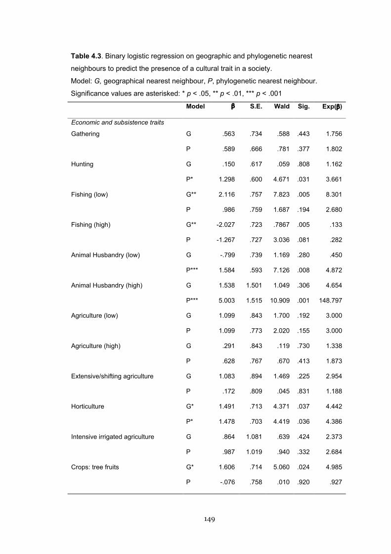
149
Table 4.3. Binary logistic regression on geographic and phylogenetic nearest
neighbours to predict the presence of a cultural trait in a society.
Model: G, geographical nearest neighbour, P, phylogenetic nearest neighbour.
Significance values are asterisked: * p < .05, ** p < .01, *** p < .001
Model β S.E. Wald Sig. Exp(β)
Economic and subsistence traits
Gathering G .563 .734 .588 .443 1.756
P .589 .666 .781 .377 1.802
Hunting G .150 .617 .059 .808 1.162
P* 1.298 .600 4.671 .031 3.661
Fishing (low) G** 2.116 .757 7.823 .005 8.301
P .986 .759 1.687 .194 2.680
Fishing (high) G** -2.027 .723 .7867 .005 .133
P -1.267 .727 3.036 .081 .282
Animal Husbandry (low) G -.799 .739 1.169 .280 .450
P*** 1.584 .593 7.126 .008 4.872
Animal Husbandry (high) G 1.538 1.501 1.049 .306 4.654
P*** 5.003 1.515 10.909 .001 148.797
Agriculture (low) G 1.099 .843 1.700 .192 3.000
P 1.099 .773 2.020 .155 3.000
Agriculture (high) G .291 .843 .119 .730 1.338
P .628 .767 .670 .413 1.873
Extensive/shifting agriculture G 1.083 .894 1.469 .225 2.954
P .172 .809 .045 .831 1.188
Horticulture G* 1.491 .713 4.371 .037 4.442
P* 1.478 .703 4.419 .036 4.386
Intensive irrigated agriculture G .864 1.081 .639 .424 2.373
P .987 1.019 .940 .332 2.684
Crops: tree fruits G* 1.606 .714 5.060 .024 4.985
P -.076 .758 .010 .920 .927
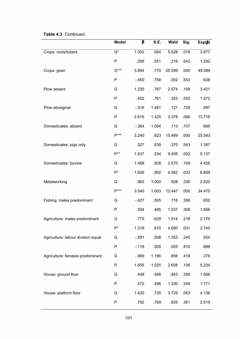
150
Table 4.3. Continued.
Model β S.E. Wald Sig. Exp(β)
Crops: roots/tubers G* 1.302 .554 5.528 .019 3.677
P .256 .551 .216 .642 1.292
Crops: grain G*** 3.894 .770 25.595 .000 49.089
P -.450 .758 .352 .553 .638
Plow absent G 1.230 .767 2.574 .109 3.421
P .452 .761 .353 .552 1.572
Plow aboriginal G -.516 1.481 .121 .728 .597
P 2.619 1.425 3.378 .066 13.716
Domesticates: absent G -.364 1.084 .113 .737 .695
P*** 3.240 .823 15.489 .000 25.543
Domesticates: pigs only G .327 .538 .370 .543 1.387
P** 1.637 .534 9.405 .002 5.137
Domesticates: bovine G 1.488 .928 2.570 .109 4.426
P* 1.926 .902 4.562 .033 6.859
Metalworking G .963 1.000 .928 .335 2.620
P*** 3.540 1.003 12.447 .000 34.470
Fishing: males predominant G -.427 .505 .716 .398 .652
P .504 .495 1.037 .309 1.656
Agriculture: males predominant G .775 .629 1.514 .218 2.170
P* 1.319 .610 4.680 .031 3.740
Agriculture: labour division equal G -.591 .508 1.353 .245 .554
P -.118 .505 .055 .815 .888
Agriculture: females predominant G -.969 1.196 .656 .418 .379
P 1.655 1.025 2.608 .106 5.234
House: ground floor G .448 .488 .843 .359 1.566
P .572 .496 1.330 .249 1.771
House: platform floor G 1.420 .735 3.729 .053 4.136
P .702 .769 .835 .361 2.019

151
Table 4.3. Continued.
Model β S.E. Wald Sig. Exp(β)
House: raised floor G 9.166 39.946 .053 .819 9563.61
P -7.740 39.948 .038 .846 .000
Hamlets G -.360 .841 .183 .669 .698
P .972 .816 1.417 .234 2.642
Compact settlements G -.763 .903 .713 .398 .466
P 1.307 .906 2.079 .149 3.693
Social and kinship traits
Brideprice G* 1.289 .591 4.749 .029 3.629
P* 1.289 .591 4.749 .029 3.629
Gift exchange for wives G 1.135 .950 1.425 .233 3.110
P -.197 1.076 .034 .855 .821
No marriage transactions G** 1.532 .573 7.146 .008 4.626
P* 1.188 .554 4.597 .032 3.280
Monogamous nuclear family G -7.530 29.870 .064 .801 .001
P .580 .888 .427 .514 1.786
Polygynous families G -.022 .591 .001 .970 .978
P .531 .545 .949 .330 1.701
Extended families G -.418 .503 .693 .405 .658
P .607 .502 1.461 .227 1.835
Monogamy G .733 .642 1.304 .254 2.081
P .733 .642 1.304 .254 2.081
Polygyny G -.169 .585 .083 .773 .845
P .956 .577 2.746 .097 2.602
Patrilocality G .209 .489 .184 .668 1.233
P .445 .496 .804 .370 1.560
Ambi/neolocality G 9.807 51.464 .036 .849 18155
P -17.67 69.814 .064 .800 .000

152
Table 4.3. Continued.
Model β S.E. Wald Sig. Exp(β)
Matrilocality G -1.109 1.017 1.189 .276 .330
P 1.451 .985 2.172 .141 4.268
Alternate form of residence G .007 .492 .000 .988 1.007
P -.483 .485 .993 .319 .617
Agamous communities G .862 .585 2.171 .141 2.369
P -.117 .583 .040 .841 .889
Segmented communities G** 1.523 .564 7.283 .007 4.584
P -.538 .573 .883 .347 .584
Single community patrilineages G 1.951 1.012 3.721 .054 7.037
P** 2.554 .900 8.050 .005 12.855
Multiple-community patrilineages G* 1.533 .685 5.010 .025 4.631
P -.242 .773 .098 .754 .785
Matrilineages G .537 .560 .919 .338 1.711
P .712 .600 1.407 .235 2.037
Cognatic descent G -.792 .533 2.207 .137 .453
P** -1.464 .540 7.342 .007 .231
Unilineal descent G .898 .540 2.773 .096 2.456
P** 1.540 .544 8.010 .005 4.665
Marriage: first and/or second cousins G* -1.004 .508 3.9110 .048 .366
P* -1.029 .522 3.882 .049 .357
Marriage: no cousins G** 1.562 .601 6.761 .009 4.768
P .360 .594 .366 .545 1.433
Preference for type of cousins G** 2.569 .972 6.982 .008 13.059
P -2.145 1.119 3.672 .055 .117
Eskimo G .556 1.118 .247 .619 1.744
P* 2.162 .963 5.039 .025 8.689

153
Table 4.3. Continued.
Model β S.E. Wald Sig. Exp(β)
Hawaiian G -.297 .518 .329 .566 .743
P .888 .524 2.870 .090 2.431
Iriquois G* 1.576 .725 4.726 .030 4.836
P -.131 .787 .028 .867 .877
Descent: patrilineal G .841 .780 1.164 .281 2.319
P .524 .807 .422 .516 1.689
Descent: matrilineal G .268 .764 .123 .726 1.308
P* 1.596 .697 5.248 .022 4.932
Descent: ambilineal G** 1.666 .614 7.367 .007 5.290
P 1.027 .609 2.845 .092 2.794
Descent: bilateral G 1.827 1.070 2.914 .088 6.217
P 1.017 .944 1.159 .282 2.764
Descent: mixed G 1.504 1.484 1.027 .311 4.500
P -8.731 36.454 .057 .811 .000
No classes G .703 .848 .689 .407 2.021
P .703 .848 .689 .407 2.021
Wealth distinction G -.384 1.126 .117 .733 .681
P* 2.230 1.055 4.468 .035 9.298
Elaborated class distinctions G .243 .543 .200 .654 1.275
P .665 .559 1.414 .234 1.944
Slavery G* 2.509 1.004 6.245 .012 12.288
P .920 .908 1.028 .311 2.510
Former presence of slavery G 1.955 1.101 3.154 .076 7.065
P* 2.406 .929 6.710 .010 11.090
Hereditary succession to office G .059 .521 .013 .909 1.061
P* .981 .519 3.569 .049 2.668
Non-hereditary succession G -.475 .510 .869 .351 .622
P 1.566 .840 3.479 .062 4.788

154
4.4.6 Nearest neighbour tests: Discussion
Using a nearest-neighbour regression method I found that phylogenetic nearest
neighbour predicted the state of slightly more cultural traits than did geographic
nearest neighbour. There was no difference between “economic” and “social” classes of
traits with respect to PNN and GNN. Compared with these results, Guglielmino et al.
(1995) found that economic traits (their “Economy” and “Social stratification”) were
explained well by all three modes of transmission, and in their later paper (Hewlett et
al. 2002) these authors found phylogeny to explain many social stratification traits.
Similarly in the present analysis, three of the four significant social stratification traits
(“wealth classes”, “former slavery”, and “hereditary succession”) were predicted by the
PNN. It is interesting to note that those traits that involve heritable resources—either
material resources, such as domesticated animals, or social resources, such as the
presence of slavery—seem to be those that show strong phylogenetic signal. It is almost
as though important parent-offspring transmission of the means of subsistence at the
micro-level is still of relevance when explaining macro-level cultural variation. This
could be construed as a form of niche construction (Laland, Odling-Smee, and
Feldman 2000), that is, whereby individuals modify the source of natural selection in
their own environment. In this case, by creating forms of heritable resources,
individuals create selection pressures for subsequent generations to continue to
transmit such a strategy vertically.
The Austronesian language family is one of several worldwide associated with
an agricultural dispersal (Diamond and Bellwood 2003). Over half of the economic
traits predicted by the PNN are concerned with animal domesticates. Archaeological
evidence from Lapita sites throughout Oceania reveal a consistent “package” of pig,
dog and chicken transported as domesticated animals (Lynch 1991; Kirch 1997;
Spriggs 1997), while the presence of bovine animals such as the Asian water buffalo
and Bali cattle appear to be concentrated in a restricted set of societies in Island

155
Southeast Asia (Lau et al. 1998). Plant-based subsistence traits, however, are
associated with geography. It may be that horticultural or crop traits diffuse more
readily than domesticated animals, being less “expensive” technologies. In addition,
crop types are more likely to be constrained by type of ecological environment they are
suited to, which may be reflected in geographical ranges. Animals, in the societies that
possess them, are frequently consumers of household waste (e.g. pigs) and not subject
to such ecological constraints. In addition, animals may represent heritable wealth,
and as such may be more likely to be conserved vertically.
Kinship traits concerning descent and inheritance were frequently associated
with phylogeny in this analysis. Descent systems (e.g. cognatic or unilineal descent)
structure patterns of relationship, defining who is kin and who is not, and to whom
rights and wealth will be accorded. As such, it is unsurprising that they follow a vertical
sort of transmission. Descent systems, especially matriliny, are the subject of later
comparative analyses (Chapters Five and Six); the results of the present analyses
demonstrate that a phylogenetic method is necessary to control for non-independence
(Galton’s Problem). However, ambilineal descent, where there is flexibility in the
kinship system such that descent can be traced through either sex, is associated with
the geographic model, and thus may co-vary adaptively with aspects of the
environment.
4.5 Cultural transmission: Discussion
4.5.1 Comparison with previous work
Using Mantel matrix tests and a nearest neighbour approach, the analyses
demonstrated that cultural trait variation was moderately but significantly correlated
with both geographic proximity and phylogenetic relationship. Both historical and
diffusion processes account for the patterns of cultural similarity in this group of
Austronesian societies. We cannot compare the Mantel correlations and nearest-

156
neighbour regression results directly, but we can compare the patterns in the findings.
Mantel tests are probably closer to the previous analyses of Guglielmino et al. and
Hewlett et al. in that they do not contain a strict, character-based control for
phylogeny, but work on overall similarities. Mantel matrix analyses here showed a
greater overall partial correlation of geographic versus phylogenetic distances with all
cultural traits; however, it appeared that economic traits were responsible for this
result. There was no association between social trait distances and geographic
distances. Compared to previous results, which have found positive evidence of a
greater relationship of social traits and a phylogenetic model, and ambiguous or low
evidence for a geographic model associated with economic traits, we found the
opposite: positive evidence for the association between geographic proximity and
economic trait similarity. It may be that in the Pacific, more marginal and/or
proscriptive environments such as atolls, where limited topsoil restricts crops to
species such as Colocasia taro and coconuts (Barrau 1961) restrict the variation
possible in subsistence systems compared to Africa, and geography thus accounts for
more of the observed similarity.
The work of previous authors did not directly compute correlations with
geographical distance but constructed a clustering index. This index indicated a similar
degree (~.30) of geographic clustering for both social and economic traits, which the
nearest-neighbour regression in the present study also found. The regression analysis
showed an equal influence of phylogenetic and geographic effects across both types of
cultural traits. Here a slightly higher effect of phylogeny was found overall, but it is not
remarkable. In neither analysis was there positive evidence for phylogenetic
transmission being of more than marginally greater importance than geographic
transmission in respect to social traits overall. However, many kinship traits were
predicted by a phylogenetic model.
A common criticism of the use of phylogenetic methods on cultural variation is
that human societies borrow, impose, and generally diffuse aspects of their culture on

157
other societies, potentially obscuring any historical signal. Geographic diffusion—trait
“borrowing”—after the initial spread of the Austronesian language family
approximately 5500 years ago (Bellwood 1997) should be expected to have the effect of
washing out the initial signature of phylogenetic relationship. Although diffusion and
adaptation are not mutually exclusive, and any trait borrowing could be for adaptive
reasons, it is unlikely that this historical signal would be renewed through any
subsequent (and exactly complementary) movements of people. Thus, any
macroevolutionary cultural analysis should expect to find at least some evidence of
geographic diffusion. We know that even in the case of the remote Polynesian islands
there was post-colonisation trade and voyaging for a least some period of time,
evidenced by the archaeological remains of volcanic glass and basalt adzes between
far-flung islands in the Marquesas and Pitcairn groups (Weisler 1998; Rolett 2002).
Given some certain degree of diffusion, it is unsurprising that the correlations with
geographical distance should equal or be greater than those with linguistic distance,
and in instances where they do not exist, in the case of social/kinship traits under the
Mantel test, can be taken as strong evidence for historical signal.
4.5.2 Consideration of the methodologies
The nearest neighbour method was a conservative test, requiring a reliable estimate of
the PNN to proceed. As such, for a number of the traits examined, the effective sample
sizes were small (~40), and we may have lost statistical power to determine effects.
The significant associations of GNN and PNN with individual cultural traits should
therefore be seen as positive evidence under a stringent test and within a regional
context. As well, they confirm the approach taken by Holden and Mace (1999) as a
useful one, as it allows us to identify those traits that require a phylogenetic method in
order to control for historical relationships.
158
Separate regression analyses (not shown) included an interaction term to
assess the degree of collinearity in the data. Interaction terms were significant in less
than one quarter of the traits, and did not consistently appear with significant
GNN/PNN predictors. Thus, there is some degree of collinearity between phylogeny
and geography, but not in every trait, and not always when another significant
predictor was found. The Mantel tests, by computing partial correlations, allowed us to
hold these interaction effects constant.
Simple linear distance measures represent the opportunities for geographic
diffusion in these analyses. Prevailing winds and currents may determine the
frequency of interaction of ocean-voyaging societies more than does simple proximity.
In addition, we cannot be certain if a unit of geographic distances across land presents
an equal conduit or barrier for interaction than the corresponding unit of distance
across the ocean. With such a widely spread language family as Austronesian, we
might assume that past a certain point all distances are equally far (and thus equally
unlikely). However, using log-transformed distances did not indicate such an effect. It
may be that societies form chains of interaction spheres, so that even though
individuals from one place do not visit or encounter individuals from a far-distance
place, cultural traits do diffuse along overlapping sets of pairwise societies. For further
resolution it would be desirable to draw from models of ocean voyaging such as Irwin
(1992) to weight sets of neighbours as more or less likely according to variables such as
currents or target island size.
4.5.3 Conclusion
Phylogenetic and geographic transmission are associated with different traits,
indicating that the type of cultural trait under study may be subject to differing
evolutionary forces. When modelling cultural transmission, we cannot assume a “one-
mode-fits-all” model. Importantly, the results of the second analysis suggest that a

159
phylogenetic model that controls for the effects of shared ancestry is relevant when
examining descent-related cultural traits, and suggests that even in vastly different
environmental and cultural contexts (Africa versus the Pacific), similar patterns of
cultural transmission may account for cultural diversity in descent traits. These issues
are explored further in the comparative analyses in Chapters Five and Six.
160
CHAPTER FIVE
ANCESTRAL STATES OF DESCENT AND RESIDENCE
Systematic comparison of Oceanic cultures should enable us toreconstruct in large measure the shape of the parent culture.
(Goodenough 1957:154)
5.1 Summary
Descent groups and post-marital residence patterns are important facets of social
organisation, as they determine where and how individuals associate with kin and
invest their resources. Descent and residence in Austronesian societies is variable and
hypotheses about the ancestral states of these traits abound in the literature, although
none have been formally tested. Here I use a Bayesian MCMC comparative method to
estimate the ancestral states of (i) descent and (ii) residence at each node in a sample
of 1000 language trees. The cultural traits are examined with both binary and multi-
state coding to tease apart the evolution of social organisation. Measures of certainty in
the ancestral states are estimated and combined with measures of phylogenetic
uncertainty. Model likelihoods vary systematically over the tree sample, indicating that
phylogenetic control is necessary. Early Austronesian social organisation is
reconstructed to have bilateral descent groups and inheritance, with matrilocal
residence. Lineal systems are later developments in the tree; patrilineality
characterises Near Oceania and Polynesia, matrilineality characterises Micronesia. The
hypothesis of matricentric kinship in Proto Oceanic society is supported by the data.
Residential flexibility is an ancient Austronesian feature. Results are interpreted in the
light of the theoretical models of Austronesian kinship and the ethnographic literature.
161
5.2 Introduction
Robin Fox began Kinship and Marriage (1967:27) with the observation that his
subjects were about “the basic facts of life”. While anthropology’s approach to what
was once its core concern has changed drastically since then (Holy 1996), becoming
particularist to the point where cross-cultural notions of kinship are regarded as
merely a product of Western bias (Schneider 1984), evolutionarily-minded social
scientists still treat kinship as fundamentally important in understanding general
principles of human social behaviour. Two aspects of kinship that can determine with
whom an individual associates are (i) descent and (ii) residence, and their rules may
influence one another. Descent systems are ways in which societies stipulate who is
and who is not kin, while residence rules state where individuals live.
5.2.1 Descent
Individuals may be genealogically related to many other people, but in most societies,
there are descent groups that circumscribe only a portion of those relatives (and
perhaps include other non-relatives) to be recognised as kin. Thus, descent systems
track the group membership of relatives one considers close kin, sometimes in a quite
different way from what simple quotients of biological relatedness would suggest
(Sanderson 2001). Inheritance, rights and obligations, the regulation of marriage, and
social and material assistance are all affected to some degree by kinship rules that
stipulate who is and is not regarded as part of one’s descent group. From an
evolutionary point of view, descent rules determine where individual invests her time
and resources, and these rules may be seen as expressing forms of parental or kin
investment (Trivers 1972; Clutton-Brook 1991). Cross-cultural variation in descent
rules thus presents an intriguing set of questions for evolutionary theory to address.
Descent systems fall into two broad categories (Fox 1967; Holy 1996). Unilineal
descent means that an individual is a member of one, non-overlapping kin group,

162
traced through either one’s father’s male ancestors (patriliny) or one’s mother’s female
ancestors (matriliny). More rarely, some societies have double descent, meaning that
both patrilineal and matrilineal groups are present; Austronesian examples include
Pukapuka in Polynesia and the Caroline Islands in Micronesia (Damas 1979).
Ambilineal descent is a special case of lineal descent where individuals choose to
affiliate with mother’s or father’s descent line without set rules (Firth 1957). This
choice may be an active consideration by an individual or their parents, or it may be
the result of gradual fulfilment of various rights and obligations that lead to adult
membership in one group at the expense of another. Ambilineal descent is found
frequently in Austronesian societies, such as Kiribati in Micronesia, where individuals
may belong to many ancestors’ descent groups, but main affiliation is determined by
the parents’ place of residence and the ongoing participation in lineage-specific
activities (Lambert 1966).
In contrast, non-unilineal descent occurs when individuals trace kin
relationships in often overlapping kin groups; these can be through ancestors of either
or both sexes. Bilateral and cognatic systems fall under this heading. Modern English
family organisation follows a bilateral principle; an individual’s network of relatives
“on either side” is unique and does not form a permanent, enduring lineage, persisting
only through her lifetime. Fox (1967:169) makes this distinction:
[W]hat matters is not so much the division into unilineal and cognatic,as the difference between the ego-focus on the one hand with itspersonal ‘groups’, and the ancestor-focus on the other with its descentgroups.
Partly as reaction to the proliferative taxonomy of descent nomenclature, in the
middle of the 20th century anthropologists suffered some anxiety over whether
ancestor-oriented yet non-unilineal societies had “descent groups” in the sense that
Africanist anthropologists had come to use the concept (Goodenough 1955; Davenport
1959; Leach 1962). These “cognatic” forms of social organisation were especially
163
common in Southeast Asian and insular Pacific societies, such as the Maori (Firth
1957; Scheffler 1964). Kirch and Green (2001) use Levi-Strauss’ (1982) “House society”
concept in their reconstruction of kinship in Ancestral Polynesian Society, as does Fox
(1993, 1995) for societies in Island Southeast Asia. Irrespective of notions of “ascent”
(Fox 1995) versus descent, and other debates about lineage models (Howard and
Kirkpatrick 1989), a House society is a social unit that is time-enduring, holds fixed
property (both land and houses), and acts as an organising principle for the
transmission of resources, be they material or social (Kirch and Green 2001). From an
evolutionary perspective, the continuity of a kin group through time, and its
association with the transmission of resources is sufficient cause to regard such
societies as having descent groups that set them aside from bilateral kin systems.
While rules of descent may determine who is kin, the rules may differ according
to the type of behaviour or purpose being specified. For instance, rules for the
inheritance of land may differ from those that determine inheritance of titles or
movable property, or obligations for assistance, or access to marriage partners. The
Lakalai of New Britain, as described by Chowning (1966), have mostly-exogamous
matrilineal units to which people belong by birth; these “sibs” share resources such as
land and a water supply, transmit certain food taboos and offer solidarity in times of
feuding. However, a person is also bound by ties of obligation to a bilateral hamlet, and
men transmit some private property such as pigs to their sons. The Lakalai consider
their matrilineal sibs to be permanent and enduring aspects of their kinship
(1966:499). Thus, although there are most certainly nuances of human social
behaviour that cannot be encapsulated with simple classification schemes, the kinship
categories described above capture a significant dimension of the cross-cultural
variation in how people organise their kin relationships. Like the simplifying
assumptions made in all forms of biological comparison, basic kinship categories are a
useful starting point for an eventual understanding of the evolutionary dynamics of

164
social organisation. Figure 5.1 shows traditional kinship diagrams representing the
common categories.
Figure 5.1. Traditional kinship diagrams. Circles represent females, triangles
represent males. Marriage relationships are denoted by = (double horizontal lines),
descent relationships by | (vertical lines) Top. Patrilineal descent, showing Ego’s
patriline in blue. Members of another patriline are shown in grey. Middle. Matrilineal
descent, showing Ego’s matriline in red. Members of another matriline are shown in
grey. Bottom. Bilateral descent, showing Ego’s kindred in yellow. In bilateral descent,
the degree of relationship fades the further up and out from Ego one progresses.

165
5.2.2 Residence
Individuals are generally affiliated with some descent group(s) at birth, but newlywed
couples face the choice of determining with whom to live, and consequently to which
group their children will belong. Thus, post-marital residence rules are related to a
society’s descent system. Patrilineal descent usually occurs with patrilocal residence,
where the wife lives with the husband’s kin. This pattern is the most common
worldwide (Murdock 1949:38), occurring in about 70 percent of societies (Levinson
and Malone 1980:101). Similarly, matrilineal descent usually occurs with matri- or
avunculocality (residence with the maternal uncle of the husband). Cognatic, bilateral,
and ambilineal descent may often co-occur with ambilocality, where newlyweds choose
with which set of parents or kin they will reside. However, while descent and residence
rules often co-vary together in a systematic fashion (Levinson and Malone 1980:102),
they do not do so exclusively (Murdock 1949:59, Table 9). This co-variation is the
subject of Chapter Six. Here, I concentrate on the separate dynamics of descent and
residence.
5.2.3 Austronesian descent and residence
The Austronesian-speaking cultures of the Pacific represent a close approximation of
the range of worldwide cross-cultural variation in descent and residence (Lane 1961).
Parts of the Austronesian world may be characterised as having predominately one
type of descent system, such as the “matrilineal sea” of Micronesia (Weckler 1953), but
the distribution of variation is not entirely regular. The diversity of descent and
residence systems in the 67-society data set is shown in Figures 5.2, 5.3, and Table 5.1.
This diversity means that Austronesian societies are a useful regional case with which
to test hypotheses about the evolution of kinship organisation.

Figure 5.2. Geographical distribution and form of descent in 67 Austronesian societies. Numbers correspond to Table 5.2
166

Figure 5.3. Geographical distribution and form of residence in 67 Austronesian societies. Numbers correspond to Table 5.2
167

Table 5.1 Types of descent and residence, and their frequencies worldwide and in the 67-society Austronesian sample.
Frequency Description
Worldwide Austronesian
Descent
Patrilineal Affiliation with kin of both sexes through father’s male line only .40 .21
Matrilineal Affiliation with kin of both sexes through mother’s female line only .16 .18
Ambilineal Affiliation with kin through either mother or father dependent on context; may be
regulated through residence and obligation
.03 .22
Duolateral Affiliation with both mother’s line and father’s line but for separate contexts .06 .16
Bilateral Affiliation with both mother’s and father’s kin irrespective of sex .35 .22
Residence
Patrilocal/Virilocal Residence with husband’s kin .70 .53
Matrilocal/Uxorilocal Residence with wife’s kin .11 .24
Avunculocal Residence with maternal uncle of husband .06 .06
Bilocal/Ambilocal/
Duolocal
Residence is established optionally with kin of either spouse .08 .13
Neolocal Residence apart from kin of both spouses .05 .03
1. Descent: Worldwide frequencies from Standard Cross-Cultural Sample (Murdock and White 1969)
2. Residence: Worldwide frequencies from Levinson and Malone (1979:101) based on Ethnographic Atlas data.

169
Table 5.1 lists definitions and frequencies for the types of descent and residence found
in the 67-society Austronesian sample. Comparing these figures with frequencies
found worldwide, the Austronesian region has higher numbers of ambilineal and
duolateral societies, as well as less patriliny. As well, there are more matrilocal and
“multilocal” residence patterns found in Austronesian cultures, and comparatively less
patrilocal residence. However, the general patterns are fairly representative of
worldwide diversity, compared with other regions such as Europe, with a
predominance of bilateral kinship, and Africa, with mostly lineal systems (Murdock
1949, Goody 1976).
5.3 Ancestral states
Cultural behaviours do not fossilise, nor do they leave clear traces in the archaeological
record, so the nature of ancestral Austronesian kinship systems remains an open
question. In order to ultimately explain the causative processes of cultural change that
have led to the observed distribution of cultural diversity, we need to estimate the
probable ancestral states of descent and residence.
Conjecture about the ancestral state of kinship systems in Austronesian
prehistory has concentrated on two stages: the early Proto Austronesian and Proto
Malayo-Polynesian stage (PAN, PMP, c. 6-4500 BP), and the development of Proto
Oceanic (POC) society, c. 3500 BP. Here, I borrow the linguistic convention of naming
a hypothetical ancestral language “Proto X” where X is a language subgroup, and
denote a hypothetical ancestral society as “Proto X” in a similar fashion. This is not to
imply that any “Proto Society” was necessarily a single homogenous entity at a defined
point in time, but, to the degree we can reconstruct ancestral forms for a group of
ethnographically attested societies, this serves as a convenient shorthand. This
approach is similar to that taken by Kirch and Green (2001) for “Ancestral Polynesian
Society”. At the very least, there is some evidence that the Proto Oceanic stage may
coincide with the archaeological horizon of the Lapita tradition, and thus may refer to

170
real populations with a degree of cultural, geographical, and biological overlap (Kirch
2000).
5.3.1 Debates in the literature: Bilateral or lineal?
One frequent point of contention is whether ancestral Austronesian societies had
bilateral or lineal descent, and, if lineal, what form of lineality. Murdock (1949:228–31,
349–350), extrapolating from his theoretical model of descent-group development
(since termed “main sequence theory” e.g. Levinson and Malone (1980)) concluded on
the basis of kinship terminologies—that is, comparative terms for family
members—that PMP and POC society lacked exogamous unilinear kin groups. He
proposed that these ancestral societies were bilateral, lacked strict lineages, and had an
Hawaiian form of social organisation, meaning that the only distinctions in kin
terminologies were on the basis of age and sex. According to Murdock, any unilineal
forms of social organisation in Austronesian societies were the product of later
developments. On culture-distributional evidence he reconstructed the ancestral
Malayo-Polynesian social system as having a bilocal extended family organisation; in
effect, residence was a choice between the husband or wife’s kin. Kroeber (1919) had
also examined kin terminology for Philippine groups and come to a similar conclusion
that their common ancestor was bilateral, without descent groups.
Goodenough (1955) reconsidered Murdock’s claims by positing that land-
owning lineages were necessarily present in PMP society because in a number of
widespread Austronesian societies, individual rights to land were associated with kin
group membership (1955:78). These groups, however, were determined by residence
and co-existed within a bilateral kin organisation structure (e.g. the Kiribati kainga,
the Ifugao ooi, and the Ulawan komu). By comparing Oceanic and Philippine societies,
Goodenough also concluded that early AN residence may have been ambilocal. He
noted that where residence became unilocal so as to clarify rights to land, it had a
direct effect on the descent system: “where residence became patrilocal or matrilocal,

171
these groups tended automatically to be transformed into patrilineal or matrilineal
sibs and lineages” (1955:80).
In contrast, Lane (1961), following suggestions by Rivers (1914) and Burrows
(1938), claimed that the bilateral descent systems present in Polynesia and other
Oceanic societies represented a breakdown of earlier unilineal organisation. He
recorded kinship patterns from Vanuatu, noting that societies previously attested as
matrilineal had residence patterns and kin terminologies that suggested a shift to
bilateral/ambilocal organisation. This shift he attributed to demographic factors,
specifically depopulation, and he saw bilateral organisation as a flexible social
response to the pressures of marginal Oceanic environments.
Linguistic work by Pawley (1979) reconstructed the POC term *kainanga to
mean “landholding descent group”, where the cognate terms for this word in other
Oceanic languages can denote the full range of descent group forms—patrilineal,
matrilineal, and cognatic (Kirch and Green 2001). The inference here is that POC
society had some form of lineal descent group associated with land tenure.
Furthermore, comparative ethnolinguistic work by Blust (1980, 1993) revisited
Murdock’s evolutionary algorithm, pointing out that on Murdock’s model PMP society
could not only be reconstructed as bilateral and Hawaiian in kin terminology, but
could equally have had ancestor-oriented (unilineal) kin groups, and a matrilateral
organisation of marriage rules. Later examination of AN sibling terms by Blust (1993a)
reiterated this argument and used comparative linguistic evidence to establish that
Van Wouden’s (1935) reconstruction of Eastern Indonesian kinship, which posited the
exchange of marriage partners between matrilaterally related groups as central to
social organisation, was indeed likely.
Comparative ethnography was the basis for Fox (1985) to conclude, like
Murdock, that early Austronesian groups in Island Southeast Asian were originally
bilateral, and that lineal systems grew out of earlier non-lineal ones. He surmised that
the Southern Philippines was the origin for lineal organisation, which became more

172
elaborate in eastern Indonesia. Burton et al. (1996), analysing social structure traits in
world ethnographic “regions” via a statistical method using principal components
analysis, concluded that Oceanic societies had a “matricentric orientation” even when
they were classified as predominately cognatic or patrilineal. Bellwood (1997)
attempted to summarise the comparative ethnographic work in this area, but could
only conclude that early AN residence and descent could be equally reconstructed as
unilinear/-local or cognatic/ambilocal. Clearly, there is as yet no consensus.
5.3.2 Were early Austronesian societies matrilineal?
In a more multi-disciplinary approach, Hage and colleagues (Hage 1998, 1999; Hage
and Marck 2001, 2003) have re-examined Murdock’s reconstructions for POC society.
They revisited the reconstruction of Oceanic kin terminologies, especially those
associated with matrilineal/matrilocal organisation, such as a distinct term for the
mother’s brother, and have argued from comparative ethnographic, distributional, and
historical linguistic evidence that POC was very likely to be unilineal, specifically,
matrilineal. In addition, Hage and Marck (2003) have used this concept of matrilineal
social organisation in POC society to address questions in Pacific molecular
anthropology. Recent genetic work highlights the differences in male- and female-
specific inherited molecules, suggesting sex-specific differences in population
interactions (Hurles et al. 2001, 2002). Molecular anthropologists have been
interested in the colonisation of the Pacific for a number of years (Sykes et al. 1995;
Melton et al. 1998; Lum and Cann 2000; Su et al. 2000), with the aim of
“triangulating” (Kirch and Green 2001) evidence from genetics with linguistic,
archaeology, and ethnography. Maternally transmitted mtDNA has for the most part
concurred with the received view (Bellwood 1991; Bellwood 1997; Green 2003) of AN
dispersal, but recent work on the paternally-transmitted Y-chromosome has suggested
that more admixture took place than previously thought, with Y-chromosome diversity

173
being much greater, much older, and more spread throughout Near Oceania (Kayser et
al. 2000; Capelli et al. 2001).
Hage and Marck (2003) argue that these molecular findings are best accounted
for in a model where POC society was matrilineal, that is, where migrating AN
speakers incorporated diverse males (and their genes) into social groups whilst
retaining a restricted, ancestral set of female-specific genetic markers. Disentangling
the different molecular signatures left by males and females will only make sense in
light of whichever kinship systems are presumed to be operating. Thus, reconstructing
descent and residence rules may shed light on the interpretation of these genetic
findings.
5.3.3 Evolutionary interpretations of kinship structure
Just as molecular anthropologists are now beginning to realise that knowledge of
kinship structure is critical for interpreting their genetic findings (Oota et al. 2001;
Wilkins and Marlowe 2006), the study of kinship itself has benefitted from
evolutionary and ecological interpretations of the adaptive nature of social
organisation. Traditional explanations for patriliny that have stressed male authority
and social control over women gain an evolutionary interpretation where women are
seen as the “ultimate scarce resource for men” (van den Berghe 1979:100). If a wealth
surplus is possible, as in a traditional agricultural or pastoralist society, men should
attempt to prioritise the use of wealth to increase their inclusive fitness by investing in
their sons, on whose reproductive success resources will have a greater effect (Trivers
and Willard 1973). They can do this by buying high quality wives (through brideprice)
and/or more than one wife (through polygyny) (Goody 1976).
Matriliny, on the other hand, is much rarer than patriliny, but is still recurrent
worldwide. Matriliny has been associated with horticulture and fishing (Aberle 1961),
and with increased levels of paternity uncertainty (Gaulin and Schelgel 1980; Flinn
1981; Hartung 1981, 1985). Modelling wealth transmission in horticultural African

174
groups, Holden, Mace, and Sear (2003) suggested that matriliny could represent a
form of daughter-biased parental investment in societies where land is abundant but
too unproductive to benefit sons more than daughters, as the degree of relationship to
daughter’s children will always be higher.
Bilateral systems, with their concentration on the nuclear family and flexibility,
are hypothesised to be prevalent in small-scale societies without large amounts of
(heritable) material wealth, such as foraging bands, and/or large-scale industrialised
societies where kinship ties are secondary to reciprocal collectives, such as government
states (Aberle 1961; ven den Berghe 1979).
5.3.4 Inferring ancestral states
At present, the ancestral states of descent and residence across the AN family remain
open questions. A new way to approach these questions is to use comparative methods
from evolutionary biology to reconstruct ancestral states. Biologists use information
about the states of characters in present-day organisms to infer the ancestral states of
those characters in the past. For example, Pfenniger et al. (2005) investigated the
evolution of the curious “shell hairs” in Trochulus snails by constructing a phylogeny
from genetic information, and plotting shell morphology and habitat features of each
species onto the tree using a comparative method. They determined that having the
shell hairs was the ancestral state for the clade, that the character had been lost three
times in the genus, and that the hairs were an adaptation to moist environments.
Bayesian estimates of ancestral states allow us to estimate the probability of a
particular trait at any node on a phylogeny, whilst also taking into account the
uncertainty of the tree topology. Here we use a Bayesian MCMC approach on the
sample of Austronesian language trees, employing a statistical method to reconstruct
ancestral states and test hypotheses about the evolution of descent and residence.
175
5.3.5 Questions
In this chapter I address the following questions:
1. Under different coding schemes, what are the ancestral states of (i) descent and
(ii) residence at each node of the phylogeny?
2. How certain can we be in those estimates?
3. Did Proto Austronesian, Proto Malayo-Polynesian and Proto Oceanic have
bilateral or lineal descent?
4. Was Proto Oceanic matrilineal and/or matrilocal?
5. In determining ancestral states, how important is it to control for the effects of
phylogenetic uncertainty?

176
5.4 Methods
5.4.1 Linguistic data
Linguistic data for phylogenetic analysis were as described in Chapter Two for the 67-
language data set.
5.4.2 Cultural data
Data on descent and residence for the 67 societies were obtained from (i) Murdock’s
(1967) Ethnographic Atlas, in updated form as an SPSS database as collated by Gray
(1999), (ii) the Encyclopaedia of World Cultures (EWC, Levinson 1993), and (iii)
Ethnic Groups of Island South-East Asia (EGI, LeBar 1975), and supplemented by the
ethnographic literature where necessary. Descent and residence were coded in a
number of different ways according to specific hypotheses and in order to unpack the
various aspects of these cultural traits. BayesMultiState, the comparative program
used in these analyses, can accept either discrete binary or multi-state coding. Both
forms were used. Tables 5.2, 5.3, and 5.4 present the data from the EA, Levinson
(1993) and LeBar (1975) used to make coding judgments for aspects of descent and
residence.

Table 5.2. Information on descent for 67 Austronesian societies.
ETHNOGRAPHIC ATLAS VARIABLES OTHER SOURCES1 CODING2
No.
Society
Name Descent3,4 Cognatic kin groups Patrilineal kin groups Matrilineal kin groups Descent information
Des
cent
Line
al
Mat
rilin
eal
aspe
ct
1 Ambon Mixed Kindreds (recent) Single-community lineages None Patrilineal clans P L O
2 Ami Matrilineal Unilineal descent groups None Multiple-community lineages Matrilineal M L M
3 Atayal Mixed Ramages: ancestor oriented Single-community lineages None Patrilineal P L O
4 Atoni Patrilineal - - - Occasional ambilineal
recruitment
P L O
5 Balinese Patrilineal Unilineal descent groups Multiple-community lineages None Patrilineal P L O
6 Belu Matrilineal Unilineal descent groups None Single-community lineages Matrilineal M L M
7 Bolaang Bilateral - - - Bilateral B B O
8 Bunun Patrilineal Unilineal descent groups Multiple-community lineages None Patrilineal P L O
9 Carolinian Matrilineal Unilineal descent groups None Multiple-community lineages - M L M
10 Chuuk Mixed Kindreds None Multiple-community lineages Matrilineal M L M
11 Dobu Matrilineal Unilineal descent groups None Multiple-community lineages Matrilineal M L M
12 Easter Is. Ambilineal Ramages: ancestor oriented None None Lineal clans
controlled territories
MP L M
13 E. Futuna Ambilineal Ramages: ancestor oriented None None Ambilineal MP L M
14 Fijiian Patrilineal Unilineal descent groups Single-community lineages None Patrilineal clans P L O
15 Hanunoo Bilateral Kindreds None None Bilateral B B O
177

Table 5.2 (Continued). Information on descent for 67 Austronesian societies.
ETHNOGRAPHIC ATLAS VARIABLES OTHER SOURCES1 CODING2
No.
Society
Name Descent3,4 Cognatic kin groups Patrilineal kin groups Matrilineal kin groups Descent information
Des
cent
Line
al
Mat
rilin
eal
aspe
ct
16 Hawaii Bilateral Ramages: ancestor oriented None None Bilateral for commoners B B O
17 Iban Bilateral Kindreds None None Bilateral B B O
18 Ili Mandiri Patrilineal Unilineal descent groups Multiple-community lineages None Patrilineal P L O
19 Ilongot Bilateral - - - Bilateral with some
“claimed memberships”
B B O
20 Javanese Bilateral Bilateral descent None None Bilateral, some matri-
inheritance
B B M
21 Kei Patrilineal Unilineal descent groups Multiple-community lineages None - P L O
22 Kerinci Matrilineal - - - Matrilineal M L M
23 Kiribati Ambilineal Ramages: ancestor oriented None None Ambilineal MP L M
24 Kodi Duolateral Unilineal descent groups Multiple-community lineages Single-community lineages - MP L M
25 Kusaie Matrilineal Unilineal descent groups None Multiple-community lineages Matrilineal M L M
26 Kwaio Mixed Kindreds Multiple-community lineages None Patrilineal P L O
27 Lakalai Mixed Kindreds None Multiple-community lineages Matrilineal M L M
28 Macassarese Ambilineal Ramages: ancestor oriented None None Bilateral B B O
29 Madurese Bilateral - - - Bilateral B B O
30 Malagasy Duolateral Unilineal descent groups Multiple-community lineages Matrilineal exogamy - MP L M
31 Malay Bilateral Kindreds None None Bilateral B B O
178
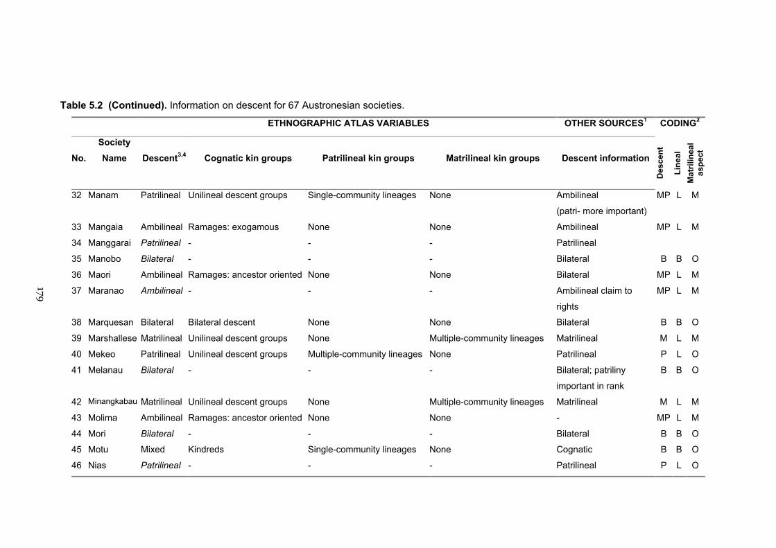
Table 5.2 (Continued). Information on descent for 67 Austronesian societies.
ETHNOGRAPHIC ATLAS VARIABLES OTHER SOURCES1 CODING2
No.
Society
Name Descent3,4 Cognatic kin groups Patrilineal kin groups Matrilineal kin groups Descent information
Des
cent
Line
alM
atril
inea
las
pect
32 Manam Patrilineal Unilineal descent groups Single-community lineages None Ambilineal
(patri- more important)
MP L M
33 Mangaia Ambilineal Ramages: exogamous None None Ambilineal MP L M
34 Manggarai Patrilineal - - - Patrilineal
35 Manobo Bilateral - - - Bilateral B B O
36 Maori Ambilineal Ramages: ancestor oriented None None Bilateral MP L M
37 Maranao Ambilineal - - - Ambilineal claim to
rights
MP L M
38 Marquesan Bilateral Bilateral descent None None Bilateral B B O
39 Marshallese Matrilineal Unilineal descent groups None Multiple-community lineages Matrilineal M L M
40 Mekeo Patrilineal Unilineal descent groups Multiple-community lineages None Patrilineal P L O
41 Melanau Bilateral - - - Bilateral; patriliny
important in rank
B B O
42 Minangkabau Matrilineal Unilineal descent groups None Multiple-community lineages Matrilineal M L M
43 Molima Ambilineal Ramages: ancestor oriented None None - MP L M
44 Mori Bilateral - - - Bilateral B B O
45 Motu Mixed Kindreds Single-community lineages None Cognatic B B O
46 Nias Patrilineal - - - Patrilineal P L O
179
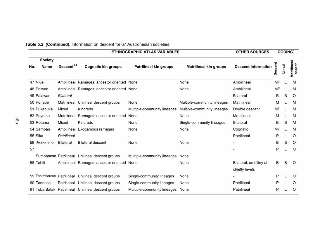
Table 5.2 (Continued). Information on descent for 67 Austronesian societies.
ETHNOGRAPHIC ATLAS VARIABLES OTHER SOURCES1 CODING2
No.
Society
Name Descent3,4 Cognatic kin groups Patrilineal kin groups Matrilineal kin groups Descent information
Des
cent
Line
al
Mat
rilin
eal
aspe
ct
47 Niue Ambilineal Ramages: ancestor oriented None None Ambilineal MP L M
48 Paiwan Ambilineal Ramages: ancestor oriented None None Ambilineal MP L M
49 Palawan Bilateral - - - Bilateral B B O
50 Ponape Matrilineal Unilineal descent groups None Multiple-community lineages Matrilineal M L M
51 Pukapuka Mixed Kindreds Multiple-community lineages Multiple-community lineages Double descent MP L M
52 Puyuma Matrilineal Ramages: ancestor oriented None None Matrilineal M L M
53 Rotuma Mixed Kindreds None Single-community lineages Bilateral B B M
54 Samoan Ambilineal Exogamous ramages None None Cognatic MP L M
55 Sika Patrilineal - - - Patrilineal P L O
56 Sugbuhanon Bilateral Bilateral descent None None - B B O
57
Sumbanese Patrilineal Unilineal descent groups Multiple-community lineages None
- P L O
58 Tahiti Ambilineal Ramages: ancestor oriented None None Bilateral; ambiliny at
chiefly levels
B B O
59 Tanimbarese Patrilineal Unilineal descent groups Single-community lineages None - P L O
60 Tannese Patrilineal Unilineal descent groups Single-community lineages None Patrilineal P L O
61 Toba Batak Patrilineal Unilineal descent groups Multiple-community lineages None Patrilineal P L O
180

Table 5.2 (Continued). Information on descent for 67 Austronesian societies.
ETHNOGRAPHIC ATLAS VARIABLES OTHER SOURCES1 CODING2
No.
Society
Name Descent3,4 Cognatic kin groups Patrilineal kin groups Matrilineal kin groups Descent information
Des
cent
Line
alM
atril
inea
las
pect
62 Tonga Ambilineal Ramages: ancestor oriented None None Patriliny; matriliny at
chiefly levels
MP L M
63 Toradja Bilateral Bilateral descent None None Bilateral B B O
64 Trobriand Matrilineal Unilineal descent groups None Multiple-community lineages Matrilineal M L M
65 Ulawa Ambilineal Ramages: ancestor oriented None None - MP L M
66 Woleai Mixed Kindreds None Multiple-community lineages Matrilineal M L M
67 Yami Bilateral Kindreds None None - B B O
1. Other Sources: Information from entries in the Encyclopaedia of World Cultures (Levinson 1980) and Ethnic Groups of Island Southeast Asia (LeBar
1975).
2. Coding. Descent: M = matrilineal P = patrilineal, MP = ambilineal/double descent/duolateral, B = bilateral/cognatic. Lineal: L = lineal, B = bilateral.
Matrilineal aspect: M = matrilineal aspect, O = no matrilineal aspect.
3. Descent: From variable “Descent” in the Ethnographic Atlas. Entries in italics are not present in the EA; these denote societies whose main form of
descent was inferred from the other sources.
4. “Mixed descent”: society has matrilineal and/or patrilineal groups present but they are not strictly unilineal.
181

Table 5.3. Information on inheritance for 67 Austronesian societies.
ETHNOGRAPHIC ATLAS VARIABLES OTHER SOURCES1 CODING2
Society Name Succession to
Headman
Inheritance of, or
access to land
Movables Inheritance Inheritance
Ambon Patrilineal heir Patrilineal (sons) Patrilineal Corporate patrilineal ownership/ inheritance of
houses/land
P
Ami Formal consensus Matrilineal (sister's sons) Matrilineal Matrilineal M
Atayal Formal consensus Patrilineal (sons) Patrilineal Patrilineal
Atoni - - - Land/heirloom property patrilineal, marriage
property (money) to spouse/children
P
Balinese Formal consensus Patrilineal (sons) Patrilineal Patrilineal P
Belu Matrilineal heir No individual property
rights
- - -
Bolaang - - - Equally amongst children, land usufruct is
village owned
-
Bunun Patrilineal heir Patrilineal (sons) Patrilineal Property inherited according to domestic
contribution
P
Carolinian - - - - -
Chuuk Matrilineal heir Patrilineal (sons) Patrilineal Land controlled by both corporate matrilines
and by individuals
MP
Dobu No such office Matrilineal (sister's sons) Matrilineal Land and movables inherited matrilineally M
182
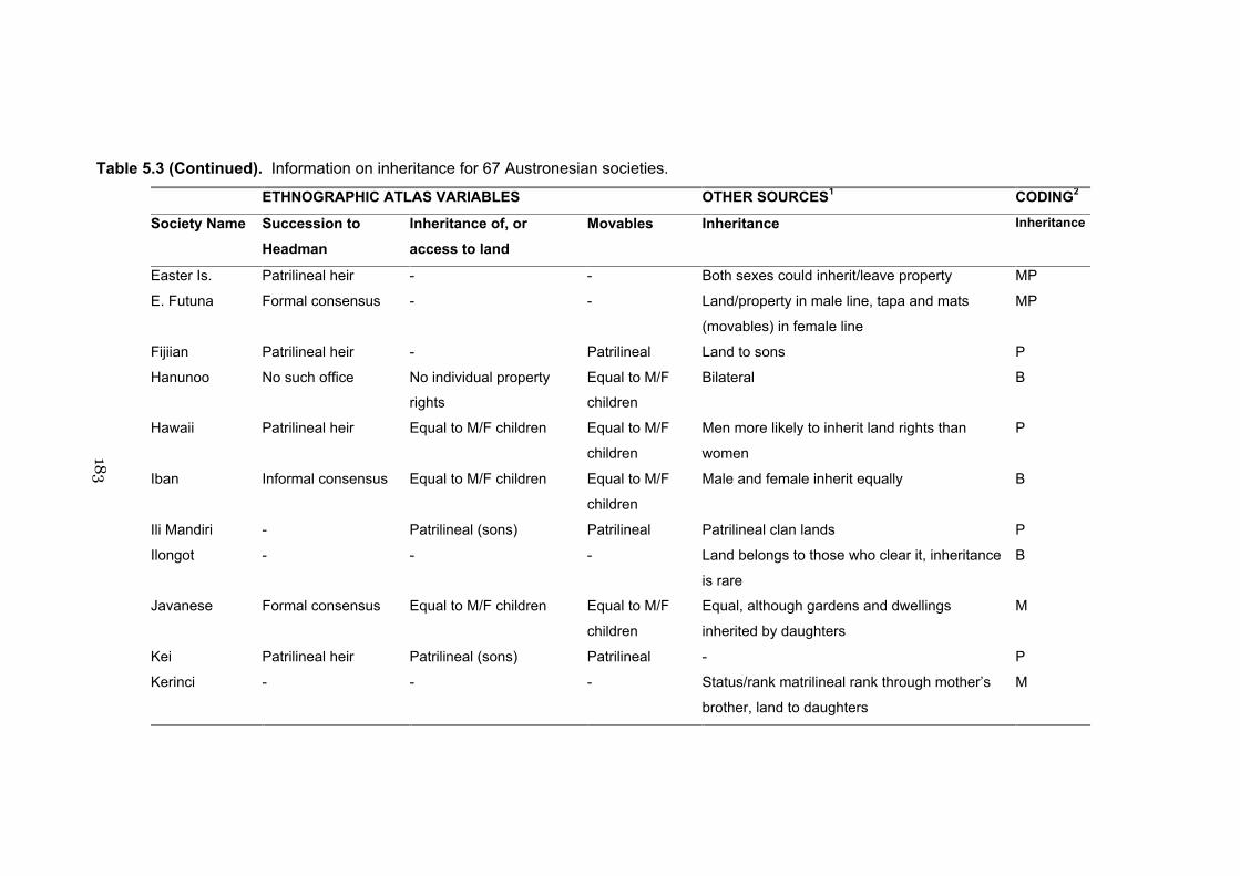
Table 5.3 (Continued). Information on inheritance for 67 Austronesian societies.
ETHNOGRAPHIC ATLAS VARIABLES OTHER SOURCES1 CODING2
Society Name Succession to
Headman
Inheritance of, or
access to land
Movables Inheritance Inheritance
Easter Is. Patrilineal heir - - Both sexes could inherit/leave property MP
E. Futuna Formal consensus - - Land/property in male line, tapa and mats
(movables) in female line
MP
Fijiian Patrilineal heir - Patrilineal Land to sons P
Hanunoo No such office No individual property
rights
Equal to M/F
children
Bilateral B
Hawaii Patrilineal heir Equal to M/F children Equal to M/F
children
Men more likely to inherit land rights than
women
P
Iban Informal consensus Equal to M/F children Equal to M/F
children
Male and female inherit equally B
Ili Mandiri - Patrilineal (sons) Patrilineal Patrilineal clan lands P
Ilongot - - - Land belongs to those who clear it, inheritance
is rare
B
Javanese Formal consensus Equal to M/F children Equal to M/F
children
Equal, although gardens and dwellings
inherited by daughters
M
Kei Patrilineal heir Patrilineal (sons) Patrilineal - P
Kerinci - - - Status/rank matrilineal rank through mother’s
brother, land to daughters
M
183

Table 5.3 (Continued). Information on inheritance for 67 Austronesian societies.
ETHNOGRAPHIC ATLAS VARIABLES OTHER SOURCES1 CODING2
Society Name Succession to
Headman
Inheritance of, or
access to land
Movables Inheritance Inheritance
Kiribati Formal consensus Children, with daughters
receiving less
Equal to M/F
children
Ambilineal land rights, associated with
residence
B
Kodi - - - - -
Kusaie - - - Modern land rights held individually -
Kwaio - - - Patrilineal P
Lakalai Informal consensus - Equal to M/F
children
Matrilineal clan lands, but wealth held by men is
used for son’s bridewealth
MP
Macassarese Patrilineal heir - - Equal to M/F children B
Madurese - - - Equal to M/F children B
Malagasy Appointment Equal to M/F children Equal to M/F
children
Equal to M/F children B
Malay - Patrilineal (sons) Equal to M/F
children
Bilateral P
Manam Patrilineal heir Patrilineal (sons) - Bilateral, more to sons P
Mangaia Patrilineal heir - - Land through male line P
Manggarai - - - Land via the patrilineage P
Manobo - - - Equal to surviving kin B
184

Table 5.3 (Continued). Information on inheritance for 67 Austronesian societies.
ETHNOGRAPHIC ATLAS VARIABLES OTHER SOURCES1 CODING2
Society Name Succession to
Headman
Inheritance of, or
access to land
Movables Inheritance Inheritance
Maori Patrilineal heir Patrilineal (sons) Patrilineal Corporate land rights, movables to same-sex
offspring
P
Maranao - - - Equal division to children, land individually
owned, usually transferred to sons
P
Marquesan Patrilineal heir Children, with daughters
receiving less
Children, with
daughters
receiving less
Emphasis on primogeniture B
Marshallese Patrilineal heir Matrilineal heirs No individual
property rights or
rules
Ambilineal; matri-clans control land tenure M
Mekeo Patrilineal heir Patrilineal (sons) - Patrilineal rights to clan lands; matrilineal
transfer of some movables
P
Melanau - - - Equal to M/F children B
Minangkabau Matrilineal heir No individual property
rights
Other matrilineal Cultivated land strictly matrilineal, some
movables transferred from father to son
M
Molima - - - - -
185
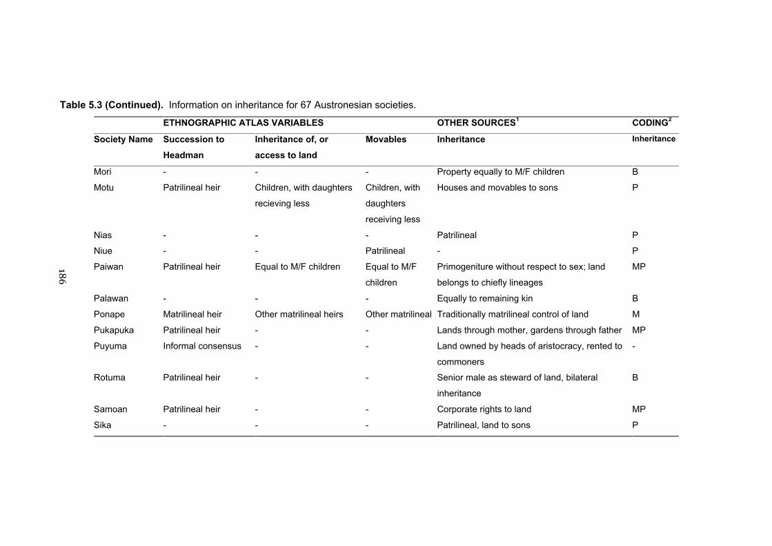
Table 5.3 (Continued). Information on inheritance for 67 Austronesian societies.
ETHNOGRAPHIC ATLAS VARIABLES OTHER SOURCES1 CODING2
Society Name Succession to
Headman
Inheritance of, or
access to land
Movables Inheritance Inheritance
Mori - - - Property equally to M/F children B
Motu Patrilineal heir Children, with daughters
recieving less
Children, with
daughters
receiving less
Houses and movables to sons P
Nias - - - Patrilineal P
Niue - - Patrilineal - P
Paiwan Patrilineal heir Equal to M/F children Equal to M/F
children
Primogeniture without respect to sex; land
belongs to chiefly lineages
MP
Palawan - - - Equally to remaining kin B
Ponape Matrilineal heir Other matrilineal heirs Other matrilineal Traditionally matrilineal control of land M
Pukapuka Patrilineal heir - - Lands through mother, gardens through father MP
Puyuma Informal consensus - - Land owned by heads of aristocracy, rented to
commoners
-
Rotuma Patrilineal heir - - Senior male as steward of land, bilateral
inheritance
B
Samoan Patrilineal heir - - Corporate rights to land MP
Sika - - - Patrilineal, land to sons P
186

Table 5.3 (Continued). Information on inheritance for 67 Austronesian societies.
ETHNOGRAPHIC ATLAS VARIABLES OTHER SOURCES1 CODING2
Society Name Succession to
Headman
Inheritance of, or
access to land
Movables Inheritance Inheritance
Sugbuhanon Formal consensus Equal to M/F children Equal to M/F
children
- B
Sumbanese Patrilineal heir Patrilineal (sons) Patrilineal
- P
Tahiti Patrilineal heir - - Male succession for lands and title P
Tanimbarese Patrilineal heir Patrilineal (sons) Patrilineal - P
Tannese Patrilineal heir Patrilineal (sons) Patrilineal Patrlineal to sons P
Tobabatak Patrilineal heir Patrilineal (sons) Patrilineal Patrilineal for land and houses P
Tonga Patrilineal heir Other patrilineal heirs - Patrilineal; traditionally land was held
corporately
P
Toradja Formal consensus Equal to M/F children Equal to M/F
children
Bilateral rights to property B
Trobriand Matrilineal heir Matrilineal (sister's sons) Matrilineal Land inherited matrilineally M
Ulawa Patrilineal heir Equal to M/F children Equal to M/F
children
- MP
Woleai Matrilineal heir - - Matrilineal corporate land M
Yami No such office Patrilineal (sons) Patrilineal - P
1. Other Sources: As for Table 5.2.
2. Coding. M = matrilineal P = patrilineal, MP = ambilineal i.e. significant transfers through separate lineages, B = bilateral/cognatic.
187
188
5.4.2.1 Coding: Descent
Multi-state coding. Three states were used (M = matrilineal, P = patrilineal, B =
bilateral/cognatic). A culture was assigned as matrilineal (n = 14) or patrilineal (n = 17)
if it were coded as such in variable 43 of the EA (“Descent: Major Type”, a code not in
the original EA but derived from variables 17, 19, and 21) or described primarily as
such in the other sources. Cultures described as ambilineal or duolateral (i.e. having
both matri- and patrilineal kin groups) were coded as MP, as the BayesMultiStates
program allows for the assignment of dual states to taxa (n = 16). Cultures described as
bilateral in v43 and having ego-oriented kindreds in v21 (“Cognatic kin groups”), or
described in the other sources as bilateral or cognatic, were coded as bilateral (n = 20).
In all coding situations, any ambiguities were resolved by cross-checking across the
three main sources or referring to the primary literature. When ambiguities were not
resolvable the society was coded as “missing” for that variable.
Inheritance of resources. Information was taken from variables concerning
inheritance in the EA (“Inheritance Rule for Real Property” “Movable Property”,
“Succession to Headman”) and other sources as described above. Three states were
used (M = matrilineal, P = patrilineal, B = equal). MP was used for societies where
some resources were transmitted patrilineally (e.g. property rights) and other
resources transmitted matrilineally (e.g. movables). Where a culture had an absence of
individual property rights, it was coded as missing (n = 7).
Lineality. Cultures were coded by the presence of lineal descent groups
(L, n = 48) or their absence (B, n = 19). Unilineal comprised all those cultures with a
matrilineal or patrilineal system of inheritance, as well as ambilineal systems, as these
imply the presence of lineal kin groups. Ambilineality, a flexible system of kinship and
inheritance rules that has been linked with changing needs in a fluctuating
environment (Fox 1967), describes a large number of Austronesian societies. Non-
unilineal comprised all societies with bilateral descent or cognatic kindreds without
lineal kin groups.
189
Matrilineality. Cultures were coded as having a matrilineal aspect (M) if they
possessed some type of matrilineal descent group (variable 19 in the EA) or some
degree of matrilineal inheritance (variables “Real Property”, “Movable Property”,
“Succession to Headman”), or similar as described in the other sources. This variable
was intended to distinguish those cultures with some aspect of matrilineal
organisation (n = 31) from strictly bilateral or patrilineal systems (n = 36).
5.4.2.2 Coding: Post-marital residence
For those cultures in the EA, I used the variable “Marital residence with kin: after first
years” as the primary indicator of residence patterns, because 48/54 cultures in the EA
were not different from earlier years. A number of coding systems were used. Table 5.4
presents residence information used to make the following coding judgements.
Primary mode of residence. Cultures were coded according to the primary
indicator in the EA or whichever was designated most common in the other sources.
Three states were used: patrilocal including virilocal, as both involve the residence
with the groom's patrilineal kin (P, n = 38), matrilocal including uxorilocal and
avunculocal (M, n = 19), or ambilocal (A, n = 10). Two neolocal cultures were coded as
ambilocal.
Scale. I constructed a five-point scale of residence from strong matrilocal
through to strong patrilocal residence. On this scale, “1” = primary residence as
matrilocal with no alternatives, strict matrilocality (n = 9); “2” = matrilocal with
alternatives, mainly matrilocal (n = 10); “3” = ambilocality or neolocality (n=12); “4” =
patrilocal with alternatives, mainly patrilocal (n=28); “5” = patrilocal with no
alternative, strictly patrilocal (n = 8).
Matrilocal option. According to Murdock's theory of kinship change (1949),
residence changes first of all aspects of social structure. Identifying those cultures with
some matrilocal aspect to their organisation provides an indicator of which cultures
may be on some transition pathway in this putative sequence. This investigation was
preparatory to the hypotheses tested in Chapter Six. A culture was coded as having a

190
matrilocal option if, in the EA, it were coded on the primary indicator as ambilocal,
matrilocal, uxorilocal, or avunculocal, or if it had an alternate or earlier form in any of
those states (n = 43). For other sources the same obtained for cultures with a
description of some matrilocal option (n = 13). In effect, this coding distinguishes
strictly patrilocal/virilocal systems (n = 11) from all others.
Flexibility. For cultures in the EA, a culture was coded flexible if it was
ambilocal in the primary indicator, possessed an alternate form of residence under the
variable "Transfer of residence at marriage: alternate form", or had a different mode of
residence in early years (n = 39). Cultures in other sources were coded as flexible if
recorded as ambilocal or if their description featured an alternative along the lines
above (n = 11). All others were coded as non-flexible (n = 17).
In summary, eight sets of analyses were conducted under the different coding
schemes: four for descent and four for residence.

Table 5.4. Information on post-marital residence for 67 Austronesian societies.
ETHNOGRAPHIC ATLAS VARIABLES OTHER SOURCES1 CODING2
Main Residence3 First years/Alternate form4 Residence information
Prim
ary
Scal
e
Flex
ibili
ty
Mat
riloc
alop
tion
Ambon Patrilocal None/Neolocal Patrilocal P 4 F O
Ami Matrilocal None/None Matrilocal M 1 N M
Atayal Patrilocal None/Matrilocal - P 4 F M
Atoni Patrilocal -/Matrilocal Virilocal with temporary uxorilocality P 4 F M
Balinese Patrilocal None/Matrilocal Patrilocal P 4 F M
Belu Matrilocal None/None Matrilocal M 1 N M
Bolaang Ambilocal -/- Ambilocal A 3 F M
Bunun Patrilocal None/None Patrilocal P 4 F M
Carolinian Matrilocal None/None - M 1 N M
Chuuk Matrilocal None/Patrilocal Matrilocal M 2 F M
Dobu Matrilocal None/None Ambilocal (matri- or avunculocal) M 3 F M
Easter Is Patrilocal None/Matrilocal - P 4 F M
E. Futuna Patrilocal Ambilocal/Matrilocal Ambilocal P 3 F M
Fijiian Patrilocal None/None Patrilocal P 4 F M
Hanunoo Matrilocal None/Patrilocal Matrilocal M 2 F M
Hawaii Ambilocal None/None Ambilocal A 3 F M
Iban Ambilocal None/None Ambilocal A 3 F M
191
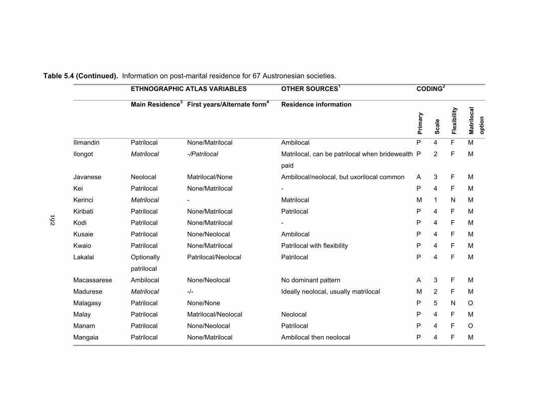
Table 5.4 (Continued). Information on post-marital residence for 67 Austronesian societies.
ETHNOGRAPHIC ATLAS VARIABLES OTHER SOURCES1 CODING2
Main Residence3 First years/Alternate form4 Residence information
Prim
ary
Scal
e
Flex
ibili
ty
Mat
riloc
alop
tion
Ilimandiri Patrilocal None/Matrilocal Ambilocal P 4 F M
Ilongot Matrilocal -/Patrilocal Matrilocal, can be patrilocal when bridewealth
paid
P 2 F M
Javanese Neolocal Matrilocal/None Ambilocal/neolocal, but uxorilocal common A 3 F M
Kei Patrilocal None/Matrilocal - P 4 F M
Kerinci Matrilocal - Matrilocal M 1 N M
Kiribati Patrilocal None/Matrilocal Patrilocal P 4 F M
Kodi Patrilocal None/Matrilocal - P 4 F M
Kusaie Patrilocal None/Neolocal Ambilocal P 4 F M
Kwaio Patrilocal None/Matrilocal Patrilocal with flexibility P 4 F M
Lakalai Optionally
patrilocal
Patrilocal/Neolocal Patrilocal P 4 F M
Macassarese Ambilocal None/Neolocal No dominant pattern A 3 F M
Madurese Matrilocal -/- Ideally neolocal, usually matrilocal M 2 F M
Malagasy Patrilocal None/None P 5 N O
Malay Patrilocal Matrilocal/Neolocal Neolocal P 4 F M
Manam Patrilocal None/Neolocal Patrilocal P 4 F O
Mangaia Patrilocal None/Matrilocal Ambilocal then neolocal P 4 F M
192

Table 5.4 (Continued). Information on post-marital residence for 67 Austronesian societies.
ETHNOGRAPHIC ATLAS VARIABLES OTHER SOURCES1 CODING2
Main Residence3 First years/Alternate form4 Residence information
Prim
ary
Scal
e
Flex
ibili
ty
Mat
riloc
alop
tion
Manggarai Patrilocal Matrilocal/- Matrilocal, patrilocal once bridewealth paid P 4 F M
Manobo Patrilocal Matrilocal/Matrilocal Brideservice then ambilocal but usually
patrilocal
P 4 F M
Maori Patrilocal None/None Patrilocal, only occasional chiefly ambilocality P 5 N O
Maranao Matrilocal -/Ambilocal Matrilocal, bridewealth payment leads to
choice
M 2 F M
Marquesan Patrilocal Matrilocal/Neolocal Patrilocal P 4 F M
Marshallese Matrilocal None/None Ambilocal M 1 N M
Mekeo Patrilocal None/None Patrilocal P 5 N O
Melanau Matrilocal - Uxorilocal M 1 N M
Minangkabau Matrilocal None/Matrilocal Couples do not establish initial common
residence
M 1 N M
Molima Patrilocal None/Avunculocal - P 4 F M
Mori Matrilocal -/Neolocal Initially matrilocal, then can be neolocal M 2 F M
Motu Patrilocal None/Matrilocal Patrilocal P 4 F M
Nias Patrilocal None/Matrilocal Patrilocal with matrilocal alternatives P 4 F M
Niue Patrilocal None/Matrilocal - P 4 F M
Paiwan Patrilocal None/Matrilocal Ambilocal P 4 F M
193

Table 5.4 (Continued). Information on post-marital residence for 67 Austronesian societies.
ETHNOGRAPHIC ATLAS VARIABLES OTHER SOURCES1 CODING2
Main Residence3 First years/Alternate form4 Residence information
Prim
ary
Scal
e
Flex
ibili
ty
Mat
riloc
alop
tion
Palawan Matrilocal -/- Uxorilocal M 2 F M
Ponape Matrilocal None/Avunculocal Ambilocal M 2 F M
Pukapuka Patrilocal None/None Patrilocal bias P 5 N O
Puyuma Matrilocal None/Patrilocal Matrilocal M 2 F M
Rotuma Matrilocal None/Avunculocal Matrilocal preference M 1 N M
Samoan Ambilocal None/None Mainly patrilocal, initially matrilocal A 3 F M
Sika Ambilocal -/- Ambilocal A 3 F M
Sugbuhanon Neolocal None/None - A 3 F O
Sumbanese Patrilocal None/None - P 5 N O
Tahiti Ambilocal None/None Ambilocal A 3 F M
Tanimbarese Patrilocal Matrilocal/None - P 4 F M
Tannese Patrilocal None/None Virilocal P 5 N O
Toba Batak Patrilocal None/Matrilocal Viriocal then neolocal is desirable P 4 F M
Tonga Patrilocal None/Avunculocal Patrilocal P 4 F M
Toradja Matrilocal None/None Ambilocal/neolocal also M 1 N M
Trobriand Matrilocal None/Patrilocal Virilocal and avunculocal M 2 F M
194
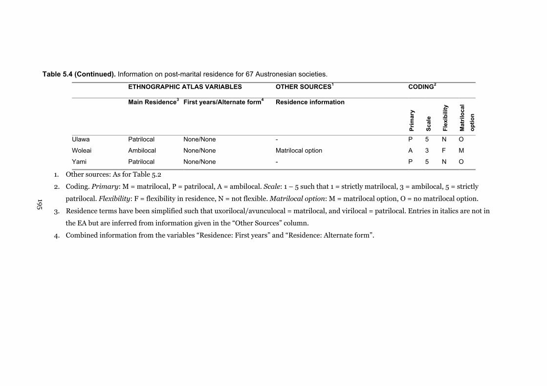
Table 5.4 (Continued). Information on post-marital residence for 67 Austronesian societies.
ETHNOGRAPHIC ATLAS VARIABLES OTHER SOURCES1 CODING2
Main Residence3 First years/Alternate form4 Residence information
Prim
ary
Scal
e
Flex
ibili
ty
Mat
riloc
alop
tion
Ulawa Patrilocal None/None - P 5 N O
Woleai Ambilocal None/None Matrilocal option A 3 F M
Yami Patrilocal None/None - P 5 N O
1. Other sources: As for Table 5.2
2. Coding. Primary: M = matrilocal, P = patrilocal, A = ambilocal. Scale: 1 – 5 such that 1 = strictly matrilocal, 3 = ambilocal, 5 = strictly
patrilocal. Flexibility: F = flexibility in residence, N = not flexible. Matrilocal option: M = matrilocal option, O = no matrilocal option.
3. Residence terms have been simplified such that uxorilocal/avunculocal = matrilocal, and virilocal = patrilocal. Entries in italics are not in
the EA but are inferred from information given in the “Other Sources” column.
4. Combined information from the variables “Residence: First years” and “Residence: Alternate form”.
195
196
5.4.3 Phylogeny estimation
BayesPhylogenies (Pagel and Meade 2004) was used to produce a 1000-tree sample
by Bayesian MCMC analysis as described in Chapter Two. All trees shown in this
chapter use the consensus tree of this sample, but the analyses themselves were
conducted on all 1000 trees.
5.4.4 Estimation of ancestral states
A continuous-time Markov model of trait evolution, implemented in the program
BayesMultiState (Pagel et al. 2004; Pagel and Meade 2005) was used to estimate the
ancestral states of descent and residence across the sample of 1000 trees. The program
takes into account uncertainty about the evolutionary scenario of cultural trait
evolution as well as the model of history proposed by the phylogeny, and was described
in detail in Chapter Three. The instantaneous rate of change between two binary traits,
for example, matrilocal option (M) and no matrilocal option (O), is measured by
transition-rate parameters qMO and qOM. These transition rates are then used to
define the probability of changes between these two states along the branches of the
tree. In the Bayesian context, a Markov chain that samples the values periodically
across the tree-sample creates a posterior probability distribution (PPD) of values of
the rate parameters (Pagel 1999). Most importantly, the ancestral state at each node
can be characterised by a PPD of each trait (e.g. M or O) whose mean and confidence
interval we can define.
As these methods estimate not only the state of the ancestral trait but account
for uncertainty in the phylogeny by summing over the tree sample, the estimated
posterior probabilities are derived by combining the probability of a state at each node
with the probability the node exists. Continuing the above example with the matrilocal
option versus no option, we may say that (i) P(n) is the probability that a node exists in
the tree sample, (ii) P(M|n) is the estimated posterior probability of a matrilocal

197
option given that the node is present, and (iii) P(M) is the probability that the node is
matrilocal taking into account the proportion of trees in which the node actually exists,
and is obtained by multiplying as follows: P(M) = P(M|n) x P(n). Conversely, we obtain
the probability of no matrilocal option, P(O), through P(O) = P(O|n) x P(n). P(n)
effectively places an upper limit on our confidence in reconstructing ancestral states.
The comparative analysis for reconstruction of ancestral states was performed
over the sample of 1000 trees on descent and residence data for 67 Austronesian
societies. In general, rates of trait switching (the transition rate parameters) were
estimated from the data rather than set to prior values. The proposal mechanism,
which the Markov chain uses as a criterion for accepting a change in the parameters,
was initially set at 50 for the binary coding and 30 for the multi-state coding.
Preliminary analyses were run to find values of the proposal mechanism that fell
between .20 and .50, meaning that between 20 and 50 percent of changes were
accepted between sampling events (M. Pagel, personal communication 2005).
Preliminary runs indicated that for some codings the data could be described well by a
wide range of parameters, thus, in order to improve the likelihoods an exponential
prior was used in some analyses to constrain the values (beta distribution with a mean
of 10; A. Meade, personal communication). For all analyses, the MCMC simulation
started from a random tree, ran for 10 million iterations, and the parameters were
sampled from the chain every 1000–10,000 iterations. This ensured that each tree was
repeatedly visited and different combinations of rate parameters were proposed. A
period of burn-in (at least 10,000) was allowed for the chain to reach convergence, and
PPD samples of the parameters, likelihoods and estimates of ancestral states at each
internal node were taken from at least 1000 iterations post-convergence.
PPD graphs for each internal node were assembled and analysed in Microsoft
Excel. The arbitrary value of .70 for combined probabilities (e.g. p(M), p(O)) was taken
as the threshold value of certainty for an ancestral state at a node, following Pagel et al.
(2004).

198
5.5 Results
5.5.1 Phylogeny
Figure 5.4 shows the consensus phylogeny of 1000 trees found by Bayesian MCMC
analysis, as reported in Chapter Two. Nodes are marked as to their posterior
probability (threshold of certainty = 70%). Certain nodes are labelled with well-known
proto-language stages, or other groupings that are particularly interesting in the
reconstruction of these cultural traits. These are referred to throughout the results and
discussion.
5.5.2 Ancestral state reconstructions
For each analysis I present (i) a colour-coded phylogeny and (ii) a set of “posterior
density” distribution panels. The phylogeny is shown annotated with reconstructed
ancestral states that have a combined probability that equals or is greater than .70.
Four or more nodes of interest are also shown as a distribution panel. These panels
plot, for those nodes, the probability of the ancestral state (from zero to one) on the x-
axis, and the number of iterations in the Markov chain with that probability on the y-
axis. They are thus the estimated posterior probability distributions of the
reconstructed state at these nodes. The distributions are derived from those trees in
which the node exists, and beneath each panel is the combined probability obtained by
multiplying the PPD of the trait by the PPD of the node, as described above in §5.4.4.
The panels are informative in the shape of their distribution, for example, panels
where the values are tightly clustered about a value indicate a great deal of robustness
in the reconstruction of the ancestral state, whereas a flattened curve spread out over
many values means a less certain reconstruction.

199
Figure 5.4. Consensus phylogeny of 1000 Bayesian trees for 67 Austronesianlanguages. Nodes are labelled as followed: PAN, Proto Austronesian; PMP, ProtoMalayo-Polynesian; PCE, Proto Central-Eastern Malayo-Polynesian, POC, ProtoOceanic, Form, Formosan, Phil, Philippine and Sulawesi, Indo, Western Indonesian;CMP Central Malayo-Polynesian; Poly, Polynesian, OCW, Oceanic (Western); Mic,Micronesian. A filled circle at the node indicates that its posterior probability is equal toor greater than .70; it is thus a node we may have some certainty of existing in morethan 70% of trees in the sample. Open circles indicate a posterior probability of lessthan .70; these nodes are phylogenetically uncertain.

200
5.5.3 Descent: Multi-state coding
5.5.3.1 Ancestral states
The ancestral state reconstruction used an exponential prior with a mean of ten, and
had a mean marginal likelihood lhharmonic = -55.63. Using multi-state coding, only 25 of
the 66 internal nodes show a combined probability greater than .70 (Figure 5.4). It
may be difficult to use multi-state coding on these data and obtain high combined
probabilities, or it may be that descent rules are actually evolving quickly on the
phylogeny, leading to uncertainty in the reconstructions. As well, a large number of
ambilineal societies, which were coded as “MP” to indicate the presence of both
matrilineal and patrilineal descent groups, may have contributed to the high
uncertainty in this particular analysis. At the root (PAN) the method reconstructs
bilateral descent as most likely (P(B) = .66), although this is not over the .70 threshold,
and the probabilities form a flattened posterior probability distribution in Figure 5.6
(top-left panel), indicating that a range of reconstructions are likely. This is further
suggested by the individual probabilities for the root, which range from .00001 to .999
for bilateral, from .00001 to .89 for matrilineal, and from .00001 to .99 for patrilineal.
The Malayo-Polynesian node (PMP) is bilateral (P(B) = .88), with the PPD
strongly skewed to high probabilities (Figure 5.6, top-right panel). WMP societies in
the Philippines and Sulawesi (node “Phil”) and Indonesia (node “Indo”) groups are
strongly bilateral, but we have less than .70 phylogenetic certainty in their ancestral
nodes. Matriliny evolves once in the Indonesian clade. As the tree branches further, the
Proto Central-Eastern (PCE) and Proto Oceanic (POC) nodes switch to patriliny. Only
at PCE is this with certainty, however, and one third of the POC reconstructions return
matriliny (Figure 5.6, middle-right panel). Polynesia (node “Poly”) continues a
patrilineal trend while containing substantial matriliny, most likely because these
societies are heavily ambilineal. Matriliny also appears in some of the other Oceanic-
Western (“OCW”) societies, especially in Micronesia where the Proto Micronesian
node (“Mic”) reaches a probability P(M) =. 98 for matriliny.

201
Figure 5.5. Ancestral state reconstruction of descent (multi-state coding) in 67
Austronesian societies. Filled nodes indicate a node reconstruction with probability
>.70. Coloured nodes indicate a state reconstruction with probability >.70 according to
the legend. Numbers above nodes indicate the state probability.

202
P(B|n) = 0.66±0.02P(B) = 0.66*1, P(P) = 0.23*1, P(M) = 0.11*1
P(B|n) = 0.88±0.01P(B) = 0.88*1, P(P) = 0.11*1, P(M) = 0.01*1
P(P|n) = 0.93±0.01P(B) = 0.02*0.99, P(P) = 0.93*0.99, P(M) = 0.05*0.99
P(P|n) = 0.52±0.02P(B) = 0.13*1, P(P) = 0.52*1, P(M) = 0.35*1
Figure 5.6. Panels showing the estimated posterior probability distribution (PPD) ofdescent with multi-state characters (bilateral, B; matrilineal, M; patrilineal, P) at fourselected nodes from the phylogeny in Figure 5.4. Below each panel is the estimatedPPD and 95% confidence intervals for the character state with the highest averageprobability (first line), and the probabilities for all three states taking into accountuncertainty about the nodes (second line). There is a switch from bilateral organisationat the base of the tree (PAN and PMP nodes) to patriliny (PCE, POC); only PMP andPCE reach the threshold of certainty. The final panel shows the PPD for all threecharacter states at the Proto Oceanic node to demonstrate the relative estimates ofthese ancestral states. There is a good deal of uncertainty about POC descent.
203
5.5.3.2 Rates of trait switching
For this analysis there were six transition rate parameters, estimated as follows: qMP=
9.86, qMB= 8.16, qPM= 11.75, qPB= 12.39, qBM= 14.39, qBP= 21.37. All were roughly
equivalent, as setting rates to be equal did not affect the marginal (harmonic) mean of
the likelihood as measured by the log-Bayes factor test (described in Chapter Three,
section §3.4.3.2). Here the Bayes factor (BF) is computed as –2*(-55.63 – -55.81) =
.36. A Bayes factor greater than 5 is evidence in support of the model being tested, so
we conclude that there is no evidence for a difference between the estimated rate
parameters and a model where they are set to be equal. If we assume the PAN root to
be bilateral, it appears more likely that societies will evolve patriliny (qBP= 21.37)
rather than matriliny (qBM= 14.39), but, as explained, the difference in the rate
parameters is not statistically significant in this case.
5.5.4 Inheritance: Multi-state coding
5.5.4.1 Ancestral states
Like descent rules, the reconstruction of multistate-coded inheritance returned less
than half the nodes (n = 25) as having a combined probability for any state greater
than .70. The ancestral state reconstruction used an exponential prior with a mean of
ten, and had a mean marginal likelihood lhharmonic = -54.97. PMP inheritance
reconstructs as bilateral P(B) = .70, but the root is uncertain (P(B) = .56), possibly due
to patrilineal inheritance in the Formosan societies Atayal, Bunun, and Paiwan. The
uncertainty about PAN is demonstrated by the flat distribution of the PPD for bilateral
inheritance, top-left panel in Figure 5.8. Bilateral inheritance with occasional matriliny
appears through the Philippines, Sulawesi, and Western Indonesia, but there is a
switch to patrilineal inheritance in Eastern Indonesia and beyond (PCE at P(P) = .92
and CMP P(P) =.90). Proto Oceanic has a patrilineal trend (P(P) = .69), again with an
underlying set of matrilineal principles (P(M) = .19) but is not certain. Patrilineal

204
inheritance strengthens in the Polynesian societies (Poly at P(P) = .98), but the sister
group of western Oceanic societies has a mixture of inheritance rules with uncertain
reconstructions. Micronesia once again reconstructs as strongly matrilineal (P(M) =
.92) in inheritance.
5.5.4.2 Rates of trait switching
The transition rate parameters (qMP= 10.67, qMB= 10.34, qPM= 7.04, qPB= 17.94, qBM=
11.93, qBP= 33.99) indicate that the least likely change is from patrilineal to matrilineal
inheritance. Setting the transition qPM to zero and comparing with the unrestricted
model returns a BF of –2.94, indicating that there is no statistical difference between
the unrestricted estimate of qPM and zero. The high rate from bilateral to patrilineal
inheritance (qBP= 33.99) can be tested if a model in which all rates are set to be equal is
compared to one where qBP is allowed to take its maximum likelihood estimate. Here
the BF = 4.32, which is evidence in favour of the high rate (Raftery 1996). Therefore, a
switch from patrilineal to matrilineal inheritance is statistically unlikely for these
societies, and bilateral inheritance is more likely to evolve into a patrilineal rather than
matrilineal system.

205
Figure 5.7. Ancestral state reconstruction of inheritance (multi-state coding) in 67
Austronesian societies. Filled nodes indicate a node reconstruction with probability
>.70. Coloured nodes indicate a state reconstruction with probability >.70 according to
the legend. Numbers above nodes indicate the state probability. Societies in grey have
missing data.

206
P(B|n) = 0.56±0.02
P(B) = 0.56*1, P(P) = 0.39*1, P(M) = 0.05*1
P(B|n) = 0.70±0.02
P(B) = 0.70*1, P(P) = 0.29*1, P(M) = 0.01*1
P(P|n) = 0.92±0.01P(B) = 0.06*0.99, P(P) = 0.92*0.99, P(M) = 0.01*0.99
P(P|n) = 0.69±0.01
P(B) = 0.12*1, P(P) = 0.69*1, P(M) = 0.19*1
Figure 5.8 PPD of inheritance with multi-state characters (bilateral, B; matrilineal, M;
patrilineal, P) at four selected nodes from the phylogeny in Figure 5.7. This figure can
be read as complimentary to Figure 5.6 (multi-state descent). As in Figure 5.6, there is
a switch from bilateral inheritance to patrilineal inheritance from earlier to later nodes,
but only PMP and PCE are statistically certain.

207
5.5.5 Descent: Lineality
5.5.5.1 Ancestral states
Binary coding, as opposed to multi-state, allowed for much more certainty in the
reconstruction of ancestral states. For this analysis, the ancestral state reconstruction
used an exponential prior with a mean of ten, and had a mean marginal likelihood
lhharmonic = -51.72. While the Formosan societies reconstruct with a lineal form of
descent group in their ancestor (node “Form”, P(L) = .94), the PAN root comes out as
bilateral (P(B) = .78), as does PMP (P(B) = .98) and the Philippine and Indonesian
societies, though the latter two are not nodes with strong phylogenetic certainty. Thus,
although the Formosan societies are basal and are all coded as lineal, the program
reconstructs the root as bilateral, possibly due to the large number of bilateral societies
in the two subsequent branches. At PCE, descent switches to lineality (P(L) = .99): the
CMP node is lineal, and all the nodes of interest in the Oceanic clade, including POC,
are lineal. The PPD panels for lineal descent in Figure 5.10 show the switch from a low
probability of lineal descent to a high probability as one progresses across the tree.
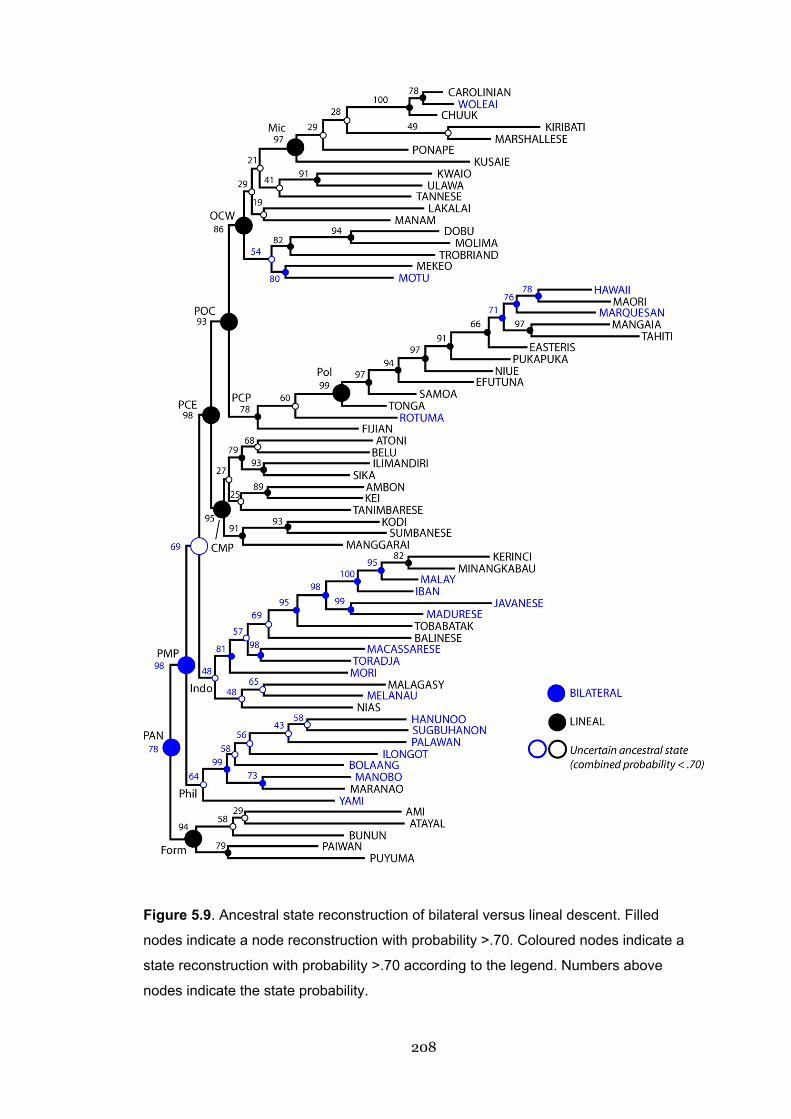
208
Figure 5.9. Ancestral state reconstruction of bilateral versus lineal descent. Filled
nodes indicate a node reconstruction with probability >.70. Coloured nodes indicate a
state reconstruction with probability >.70 according to the legend. Numbers above
nodes indicate the state probability.

209
P(L|n) = 0.22±0.01
P(L) = 0.22*1, P(B) = 0.78*1
P(L|n) = 0.02±0.00
P(L) = 0.02*1, P(B) = 0.98*1
P(L|n) = 0.99±0.00
P(L) = 0.99*0.99, P(B) = 0.01*0.99
P(L|n) = 0.93±0.01
P(L) = 0.93*1, P(B) = 0.07*1
Figure 5.10. PPD of bilateral (B) versus lineal (L) descent at four selected nodes from
the phylogeny in Figure 5.9. All panels show the PPD of ancestral states for lineality.
The early nodes are bilateral (PAN, PMP), but there is a switch to lineality between the
Indonesian societies (not shown) and PCE/POC, which reconstruct as lineal. At the
root of the tree (PAN) there is more uncertainty in the reconstruction, possibly because
the Formosan societies’ ancestor (Figure 5.9) is reconstructed as lineal.

210
5.5.5.2 Rates of trait switching
The switch from bilateral to lineal is more frequent than the reverse switch if we
compare the transition rate parameters qBL = 26.96 and qLB = 8.09. Setting the rates to
be equal, a Bayes factor test shows that there is statistical evidence for the difference
(qLB = qBL, BF = 27.92). Setting qBL = 0, thus forcing the root to be lineal, returns a BF
of –11.6. A BF of less than zero provides evidence for the unrestricted model (in this
case, where the parameters take their maximum likelihood estimates and are not
equivalent), indicating that there is no evidence that the root is lineal, even accounting
for phylogenetic uncertainty. Gaining a lineal system from a bilateral one appears to be
the probable evolutionary pathway in these societies.
5.5.6 Descent: Matrilineal aspect
5.5.6.1 Ancestral states
The ancestral state reconstruction used an exponential prior with a mean of ten, and
had a mean marginal likelihood lhharmonic = -57.13. From the root (PAN, P(O) = .86)
through PMP (P(O) = .86), to PCE (P(O) = .89) and the CMP node (P(O) = .95), the
nodes are reconstructed as having “no matrilineal aspect” in descent. This is reflect in
the first three PPD panels of Figure 5.12. The Formosan node reconstructs with the
matrilineal aspect (P(M) = .71), as does POC (P(M) = .78) and other labelled nodes in
the Oceanic societies, e.g. Micronesian (P(M) = .98). The matrilineal aspect evolves
more than once in the Austronesian family, possibly at least seven separate times, but
most notably at Proto Oceanic, where it is retained by most societies and lost
approximately four times.

211
Figure 5.11. Ancestral state reconstruction of a matrilineal aspect in descent versus
no matrilineal aspect. Filled nodes indicate a node reconstruction with probability >.70.
Coloured nodes indicate a state reconstruction with probability >.70 according to the
legend. Numbers above nodes indicate the state probability. The matrilineal aspect
appears to evolve a number of times in western Pacific societies, then once at the
POC node and be lost sporadically thereafter.
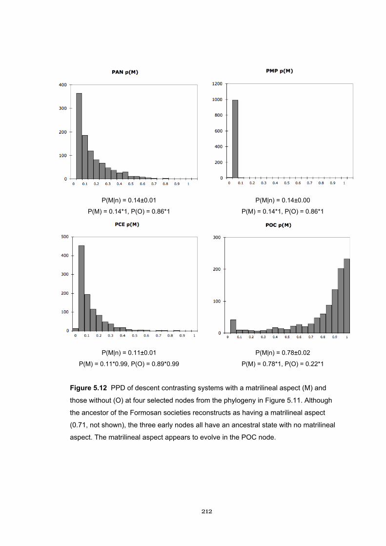
212
P(M|n) = 0.14±0.01
P(M) = 0.14*1, P(O) = 0.86*1
P(M|n) = 0.14±0.00
P(M) = 0.14*1, P(O) = 0.86*1
P(M|n) = 0.11±0.01
P(M) = 0.11*0.99, P(O) = 0.89*0.99
P(M|n) = 0.78±0.02
P(M) = 0.78*1, P(O) = 0.22*1
Figure 5.12 PPD of descent contrasting systems with a matrilineal aspect (M) and
those without (O) at four selected nodes from the phylogeny in Figure 5.11. Although
the ancestor of the Formosan societies reconstructs as having a matrilineal aspect
(0.71, not shown), the three early nodes all have an ancestral state with no matrilineal
aspect. The matrilineal aspect appears to evolve in the POC node.

213
5.5.6.2 Rates of trait switching
The transition rates between the states of having and not having a matrilineal aspect
are similar (qMO= 14.08, qOM= 19.46) and setting them to be equal makes no difference
to the likelihoods, as the Bayes factor is only 1.2. Setting qOM to zero, which forces the
root to have the matrilineal aspect, returns a BF of –12.94 in favour of the model
without the restriction. This means that the estimate of the root as having no
matrilineal aspect is strongly supported by the data, but that the trait is free to vary
across the phylogeny in both directions.
5.5.7 Residence: Scale
5.5.7.1 Ancestral states
In this analysis residence was coded on a five point scale, with “1” the matrilocal end,
“5” the patrilocal end, and “3” representing ambilocality. When ancestral states were
estimated, only six of the nodes had a posterior probability over the .70 threshold of
certainty, so the tree and PPD panels are not shown. Results are however reported in
the summary in Table 5.5. Two nodes in the Polynesian clade reconstructed as mainly
patrilocal (“4”) at combined probabilities of P(4) = .85 and P(4) = .87, as did PCE (P(4)
= .82) and CMP (P(4) = .77). The parent node of Kerinci and Minangkabau
reconstructed as strictly matrilocal at P(1) = .96, and the Philippine/Sulawesi node
(excluding Yami) reconstructed as mainly matrilocal at P(2) = .74. With five character
states, 20 rate parameters needed to be simultaneously estimated. It is likely that the
analysis did not reach equilibrium as even after 50 x 106 iterations the likelihoods
fluctuated widely (mean marginal likelihood lhharmonic = -105.96), even when
constrained with an exponential prior.
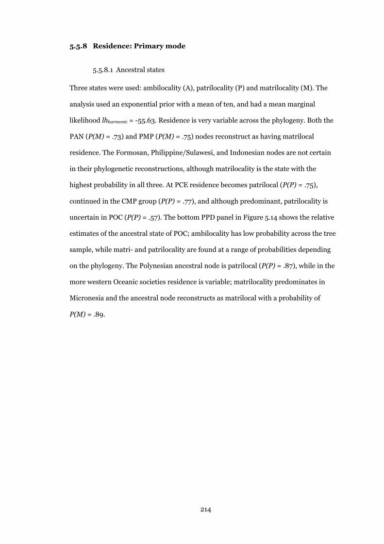
214
5.5.8 Residence: Primary mode
5.5.8.1 Ancestral states
Three states were used: ambilocality (A), patrilocality (P) and matrilocality (M). The
analysis used an exponential prior with a mean of ten, and had a mean marginal
likelihood lhharmonic = -55.63. Residence is very variable across the phylogeny. Both the
PAN (P(M) = .73) and PMP (P(M) = .75) nodes reconstruct as having matrilocal
residence. The Formosan, Philippine/Sulawesi, and Indonesian nodes are not certain
in their phylogenetic reconstructions, although matrilocality is the state with the
highest probability in all three. At PCE residence becomes patrilocal (P(P) = .75),
continued in the CMP group (P(P) = .77), and although predominant, patrilocality is
uncertain in POC (P(P) = .57). The bottom PPD panel in Figure 5.14 shows the relative
estimates of the ancestral state of POC; ambilocality has low probability across the tree
sample, while matri- and patrilocality are found at a range of probabilities depending
on the phylogeny. The Polynesian ancestral node is patrilocal (P(P) = .87), while in the
more western Oceanic societies residence is variable; matrilocality predominates in
Micronesia and the ancestral node reconstructs as matrilocal with a probability of
P(M) = .89.

215
Figure 5.13. Ancestral state reconstruction of the primary mode of residence (multi-
state coding). Filled nodes indicate a node reconstruction with probability >.70.
Coloured nodes indicate a state reconstruction with probability >.70 according to the
legend. Numbers above nodes indicate the state probability.

216
P(M|n) = 0.73±0.01P(A) = 0.09*1, P(P) = 0.18*1, P(M) = 0.73*1
P(M|n) = 0.75±0.01P(A) = 0.09*1, P(P) = 0.16*1, P(M) = 0.75*1
P(M|n) = 0.18±0.01P(A) = 0.05*0.99, P(P) = 0.75*0.99, P(M) = 0.18*0.99
P(M|n) = 0.36±0.04P(A) = 0.07*1, P(P) = 0.57*1, P(M) = 0.36*1
Figure 5.14 PPD of the primary mode of residence with multi-state characters(ambilocal, A; matrilocal, M; patrilocal, P) at three selected nodes from the phylogenyin Figure 5.13. Nodes are contrasted on their reconstruction of matrilocality.Matrilocality appears to be ancestral to the Austronesian family with increasingamounts of patrilocality appearing in the later nodes. The final panel shows the PPDfor all three character states of residence at the Proto Oceanic node to demonstratethe relative estimates of these ancestral states.

217
5.5.8.2 Rates of trait switching
Six transition rate parameters were estimated for the three states as follows:
(qMP = 35.67, qMA = 18.13, qPM = 11.12, qPA = 10.83, qAM = 20.71, qAP = 26.94). The highest
rate is from matrilocal to patrilocal, and the two lowest rates are those leading away
from patrilocality. Patrilocality may thus be some sort of “attractor” state that is easy to
get into but hard to change, which makes sense given the ubiquitous appearance of
patrilocality in all groups on the tree. This was tested by setting qPM = qPA = 0 and
comparing this model with the model where parameters take their maximum
likelihood estimates. If the two models are equivalent (BF <5) we have evidence that
the rate of change away from patrilocality is effectively zero. The BF was 2.16,
supporting this hypothesis. Additionally, I tested a model where qMP = qMA = 0, which
forced the root to be a state other than matrilocal. Here, the BF was –16.62, indicating
that there was much more support for the unrestricted model where the root was
matrilocal.
5.5.9 Residence: Matrilocal aspect
5.5.9.1 Ancestral states
No prior was used in this analysis as the range of values explored in preliminary runs
was acceptably constrained. The mean marginal likelihood was lhharmonic = -39.72.
Many more societies had a matrilocal option than did not (56 versus 11) and this state
reconstructed with high probabilities throughout much of the tree. As with the multi-
state primary mode of residence analysis, the root had the matrilocal aspect (P(M) =
.78). Examining the PPD panels shows that PAN was more variable in the range of
probabilities than PMP, where the reconstruction was constrained to a narrower range
of probabilities with a mean of P(M) = .81. PCE and POC are not certain in their
reconstructions, though they show a trend towards the matrilocal option. We can
compare this with the multi-state analysis where PCE was patrilocal and POC

218
uncertain, trending towards patrilocality. Micronesian and Polynesian are matrilocal at
P(M) = .82 and P(M) = .93 respectively. Even the strongly patri-biased CMP group
shows a trend towards the matrilocal option in the parent node (P(M) = .65). However,
it should be noted that this coding captured any aspect of matrilocality in residence,
not just the predominant mode for the society.
5.5.9.2 Rates of trait switching
Gaining the matrilocal option has a higher transition rate than losing it: qOM = 70.12
compared with qMO = 21.66. Setting the rates to be equal, a Bayes factor test shows that
there is statistical evidence for the difference (BF = 7.6, favouring the unrestricted
model); thus, gaining a matrilocal option in residence will be likely when the parent
node does not have the matrilocal option. Setting qOM = 0 and so forcing the root to
have no matrilocal option returns a BF of 18.38 in favour of the unrestricted model,
indicating that there is strong statistical evidence that PAN did indeed have the
matrilocal option.

219
Figure 5.15. Ancestral state reconstruction of a matrilocal residence option versus no
matrilocal option. Filled nodes indicate a node reconstruction with probability >.70.
Coloured nodes indicate a state reconstruction with probability >.70 according to the
legend. Numbers above nodes indicate the state probability.
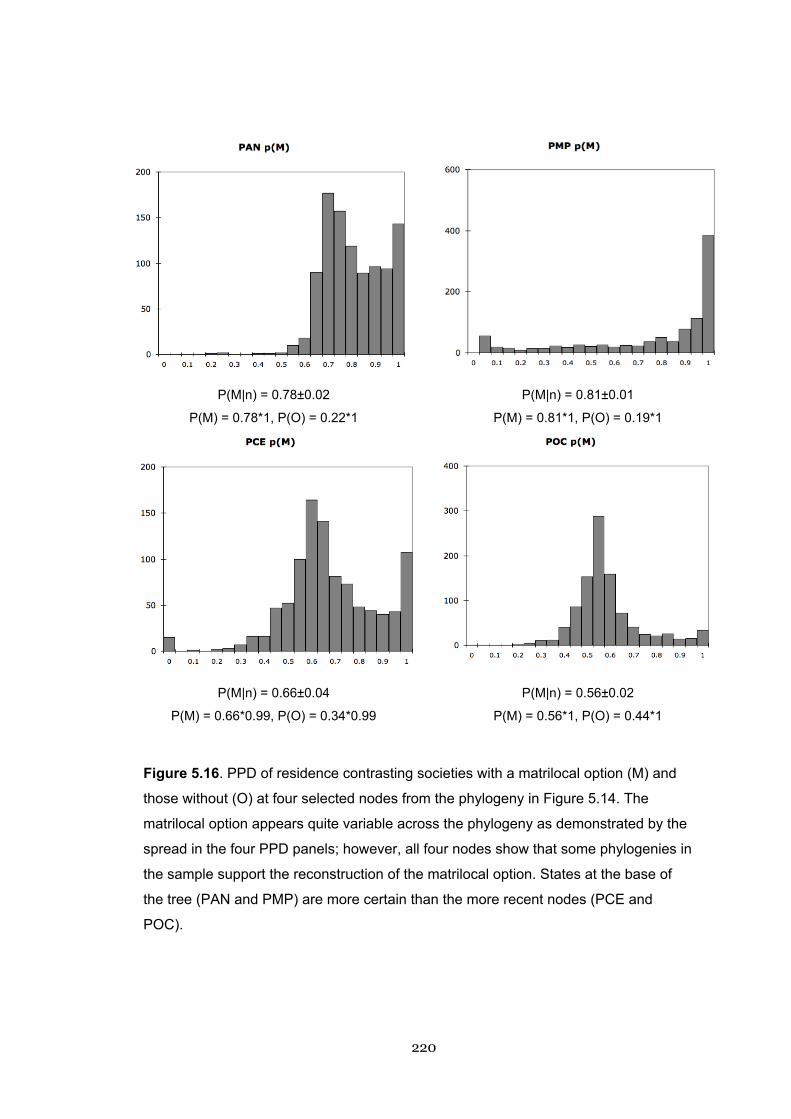
220
P(M|n) = 0.78±0.02
P(M) = 0.78*1, P(O) = 0.22*1
P(M|n) = 0.81±0.01
P(M) = 0.81*1, P(O) = 0.19*1
P(M|n) = 0.66±0.04
P(M) = 0.66*0.99, P(O) = 0.34*0.99
P(M|n) = 0.56±0.02
P(M) = 0.56*1, P(O) = 0.44*1
Figure 5.16. PPD of residence contrasting societies with a matrilocal option (M) and
those without (O) at four selected nodes from the phylogeny in Figure 5.14. The
matrilocal option appears quite variable across the phylogeny as demonstrated by the
spread in the four PPD panels; however, all four nodes show that some phylogenies in
the sample support the reconstruction of the matrilocal option. States at the base of
the tree (PAN and PMP) are more certain than the more recent nodes (PCE and
POC).

221
5.5.10 Residence: Flexibility
5.5.10.1 Ancestral states
The analysis used an exponential prior with a mean of ten and had a mean marginal
likelihood lhharmonic = -44.14. Many societies (50/67) had a flexible system of residence,
and flexibility was reconstructed as the ancestral state with high probabilities over
much of the tree. All four of the main nodes in the PPD panels show a narrow range of
high probabilities in favour of flexible residence.
5.5.10.2 Rates of trait switching
Gaining flexibility in residence has a higher transition rate than losing it, although the
difference is slight: qNF = 24.15 compared with qFN = 19.24. Setting the rates to be
equal, a Bayes factor test shows that these rates are functionally equivalent as there is
no statistical evidence for the difference (BF = .74). Setting qNF = 0, thus forcing the
root to be a strictly proscriptive residence system without flexibility, returns a BF of
–21.52 in favour of the unrestricted model, indicating that there is strong statistical
evidence that PAN had flexible residence.

222
Figure 5.17. Ancestral state reconstruction of flexible versus non-flexible systems of
residence. Filled nodes indicate a node reconstruction with probability >.70. Coloured
nodes indicate a state reconstruction with probability >.70 according to the legend.
Numbers above nodes indicate the state probability.

223
P(F|n) = 0.95±0.00
P(F) = 0.95*1, P(O) = 0.05*1
P(F|n) = 0.96±0.00
P(F) = 0.96*1, P(O) = 0.04*1
P(F|n) = 0.96±0.00
P(F) = 0.96*0.99, P(O) = 0.04*0.99
P(F|n) = 0.89±0.01
P(F) = 0.89*1, P(O) = 0.11*1
Figure 5.18 PPD of flexible (F) versus non-flexible (O) systems of residence at four
selected nodes from the phylogeny in Figure 5.17. Flexibility in residence appears to
be a trait ancestral to all Austronesian societies.

224
Table 5.5 Summary table of ancestral state reconstructions at four deep nodes: Proto
Austronesian (PAN), Proto Malayo-Polynesian (PMP), Proto Central-Eastern Malayo-
Polynesian (PCE), and Proto Oceanic. Values are the combined posterior probabilities
of each node, i.e., the probability of the state multiplied by the probability of the node.
Values in bold are those over the threshold of certainty (.70), whereas values in italics
do not reach .70 but are the highest value reconstructed for that node. Definitions of
each state class are described in the methods.
PAN PMP PCE POC
Descent groups Bilateral .66 .88 .02 .13
Matrilineal .11 .01 .05 .35
Patrilineal .23 .11 .93 .52
Inheritance Bilateral .56 .70 .06 .12
Matrilineal .05 .01 .01 .20
Patrilineal .39 .29 .93 .68
Lineality Bilateral .78 .98 .01 .07
Lineal .22 .02 .98 .93Matrilineal aspect Present .14 .14 .10 .78
Not present .86 .86 .89 .22
Residence Patrilocal .18 .16 .75 .57
Matrilocal .73 .75 .18 .36
Ambilocal .09 .09 .05 .07
Residence scale Strictly matrilocal .26 .26 .07 .15
Mainly matrilocal .19 .21 .01 .06
Ambilocal .15 .17 .07 .13
Mainly patrilocal .38 .32 .82 .57
Strictly patrilocal .03 .04 .02 .09
Flexibility in residence Flexibility .95 .96 .96 .89
No flexibility .05 .04 .03 .11
Matrilocal aspect Present .78 .81 .67 .56
Not present .22 .19 .33 .44

225
5.5.11 Summary of ancestral states results
A number of consistent patterns can be drawn out from these analyses. First, early
Austronesian descent and inheritance appear to be bilateral. Both the PAN root and
the PMP node reconstruct as bilateral as opposed to lineal, and under multi-state
analysis PMP has a high probability of being bilateral. Second, lineal descent appears
to characterise PCE and POC, so that any lineal systems in the western Pacific
(Indonesia, the Philippines, and Sulawesi) may be of later development. Third,
matrilocality seems to be present in early Austronesian society, with patrilocal systems
coming to predominate in the CMP groups of Eastern Indonesia, and in Polynesia.
However, and fourthly, residential flexibility is an ancestral and predominant
characteristic of Austronesian societies.
5.5.12 Was Proto Oceanic matrilineal and/or matrilocal?
Only three states are statistically certain for Proto Oceanic (i) a lineal descent system,
(ii) a matrilineal aspect to descent, and (iii) flexibility in residence (Table 5.5).
However, besides reconstructing the Proto Oceanic node directly, BayesMultiStates
allows us to test the hypothesis that POC was matrilineal and/or matrilocal by using a
“fossil” command (BayesMultiStates manual, http://www.evolution.rdg.ac.uk). This
elegant test compares two models: an unrestricted model where parameters take their
maximum likelihood estimates, and a model where the POC node is fixed, or fossilised,
to a selected character state, in this case matriliny or matrilocality. Using the Bayes
factor, we then compare the mean marginal likelihoods of the two models to determine
if fossilisation makes the likelihood worse than in the unrestricted model. If the
likelihood is not worsened by fossilisation, then we cannot rule out matri-centric
descent and residence in POC, even when the ancestral state estimates have returned
uncertain probabilities. The results of the fossilisation tests are presented in Table 5.6.
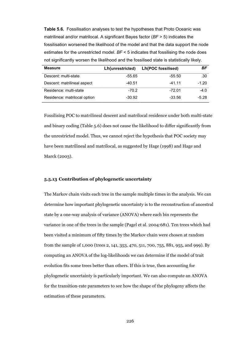
226
Table 5.6. Fossilisation analyses to test the hypotheses that Proto Oceanic was
matrilineal and/or matrilocal. A significant Bayes factor (BF > 5) indicates the
fossilisation worsened the likelihood of the model and that the data support the node
estimates for the unrestricted model. BF < 5 indicates that fossilising the node does
not significantly worsen the likelihood and the fossilised state is statistically likely.
Measure Lh(unrestricted) Lh(POC fossilised) BF
Descent: multi-state -55.65 -55.50 .30
Descent: matrilineal aspect -40.51 -41.11 -1.20
Residence: multi-state -70.2 -72.01 -4.0
Residence: matrilocal option -30.92 -33.56 -5.28
Fossilising POC to matrilineal descent and matrilocal residence under both multi-state
and binary coding (Table 5.6) does not cause the likelihood to differ significantly from
the unrestricted model. Thus, we cannot reject the hypothesis that POC society may
have been matrilineal and matrilocal, as suggested by Hage (1998) and Hage and
Marck (2003).
5.5.13 Contribution of phylogenetic uncertainty
The Markov chain visits each tree in the sample multiple times in the analysis. We can
determine how important phylogenetic uncertainty is to the reconstruction of ancestral
state by a one-way analysis of variance (ANOVA) where each bin represents the
variance in one of the trees in the sample (Pagel et al. 2004:681). Ten trees which had
been visited a minimum of fifty times by the Markov chain were chosen at random
from the sample of 1,000 (trees 2, 141, 353, 470, 511, 700, 755, 881, 955, and 999). By
computing an ANOVA of the log-likelihoods we can determine if the model of trait
evolution fits some trees better than others. If this is true, then accounting for
phylogenetic uncertainty is particularly important. We can also compute an ANOVA
for the transition-rate parameters to see how the shape of the phylogeny affects the
estimation of these parameters.

227
Table 5.7. Estimates of the between- and within-tree components of variance in
ancestral state reconstruction of descent (multi-state coding), given for the log-
likelihood and a transition-rate parameter (qBM). Ten randomly chosen trees which
were visited 50 times each by the Markov chain were used for each ANOVA.
Measure Mean square
between trees
Mean square
within trees
F
(MSB/MSW)
p-value
Log-likelihood 6.29 (df=9) 1.41 (df=480) 4.46 >.0001
qBM 239.5 (df=9) 61.62 (df=480) 3.89 >.0001
Table 5.7 shows how the log-likelihood and a rate parameter are affected by the tree
used to estimate them; the ANOVA is highly significant, indicating that controlling for
phylogenetic uncertainty is very important.
5.6 Discussion
A decade ago, reconstructing the social organisation of ancestral populations was
considered a fanciful and “unreal” enterprise for Pacific prehistorians (Sutton 1996),
even though careful extrapolation from archaeology, ethnography, and historical
linguistics—the “triangulation” approach (Kirch and Green 2001)—has allowed
anthropologists to make rich inferences about past societies (e.g. Blust 1986/87; Hage
1998, 1999; Pawley and Green 1984). However, none of this work has used an
explicitly phylogenetic approach to control for Galton’s Problem. Now, new Bayesian
comparative methods from evolutionary biology have allowed us to reconstruct the
probable ancestral states of post-marital residence and descent in Austronesian
societies. Crucially, the comparative method has allowed us to quantify the uncertainty
in these reconstructions, and to statistically test hypotheses in a scientific framework.
Proto Austronesian and Proto Malayo-Polynesian society was found to be
bilateral, without a matrilineal aspect to descent, but with (flexibly) matrilocal
residence. In the context of the literature, these results walk a middle line. Murdock
(1949), Fox (1993), and Goodenough (1955) all argued for bilaterality in PMP society.
However, beginning with Goodenough (1955), many anthropologists and linguists

228
have argued that some sort of lineal descent group, possibly matrilineal but definitely a
land-owning corporate, may have also been present in PMP society (Lane 1961; Blust
1980, 1993b; Hage 1998). The results here strongly suggest that matrilocality is
ancestral to the AN family, but not matriliny. Linguistic reconstruction using kin
terminology, which preserves relict aspects of older kinship systems, is the main
evidence for PAN/PMP matriliny; future comparative work using kin terms (e.g.
Marck 2006) should provide a more precise “fossil set” for phylogenetic
reconstruction. Moreover, the ABV language now contains more Formosan languages
with updated cognate judgements (R. Gray, personal communication); as they function
as the outgroup, the cultural-trait coding of these societies is crucial in determining the
state of residence and descent in PAN and PMP.
5.6.1 Austronesian matriliny
Lineal descent groups are reconstructed for both Proto Central-Eastern Malayo-
Polynesian and Proto Oceanic; strongly patricentric in descent, inheritance, and
residence for PCE, but uncertain for POC. However, a matrilineal aspect to descent is
strongly supported for POC, though not matrilocality. Fossilising the POC node to
matrilineal and matrilocal did not worsen the likelihood of the evolutionary model in
all cases; this study then adds to those (Lane 1961; Burton et al. 1996; Hage 1998; Hage
and Marck 2003) that have adduced matrilineality and/or matrilocality in POC society.
This is an attractive hypothesis for two reasons.
First, matrilineal social organisation in POC/Lapita peoples (Shutler and
Marck 1975; Pawley and Green 1994; Kirch 1997) would result in relatively restricted
female genetic diversity, and increased male diversity due to in-marrying men, thus
providing a framework in which to interpret the divergent mtDNA and Y-chromosome
findings in Pacific molecular anthropology (Hage and Marck 2003). Taking kinship
structure into account is crucial (Wilkins and Marlow 2006), as human genetic
diversity in the Pacific is thoroughly scrutinised, being regarded as pivotal in

229
contributing to debates over human population prehistory (Hurles et al. 2002; Hurles
et al. 2003). Secondly, a matricentric social organisation may be adaptive for voyaging
or colonising populations, as well as those with high rates of male absence through
warfare, trade, raiding, or fishing. The putative POC, and possibly PCE/PMP,
populations may correspond to points in archaeological time when significant
Austronesian expansion into new territories took place (Anderson 2002; Green 2003).
If matrilocality is an “emergency response” to male absence or mortality, and becomes
institutionalised if the emergency (such as warfare or protracted migration) persists,
then the adoption of matricentric kinship make sense (Harris 1979). Keegan and
Maclachan (1989) have argued a similar model for prehistoric Taino societies in the
Bahamas: that matricentric kinship developed in response to ongoing pathfinding and
migration throughout the West Indies that left women at home. The “male absence”
theory is investigated further in the next chapter.
5.6.2 Flexible kinship systems
While residence and descent patterns were clustered, they also showed flexibility,
switching back and forth a number of times on the phylogenies. For example, a
matrilineal aspect in descent evolved at least four times, then to be lost in daughter
societies. Flexibility in residence is apparently an ancestral Austronesian feature, with
few societies having strictly proscriptive forms of residence. The cultural ecologists
Vayda and Rappaport (1962) wrote that cultural traits in an island context were all
about “getting people to resources and resources to people” (1962:137); if kin ties are
traced flexibly, individuals and families have more options in times of uncertainty. For
example, in New Britain, the Lakalai live in region of tectonic instability and volcanic
activity that can render farmland unproductive. Disease epidemics can also depopulate
villages (Goodenough 1962). While the Lakalai have matrilineal clans, they also have
bilateral groups and flexible residence, which Goodenough proposed were
“adjustments to a series of catastrophes in fairly recent times … [this] common
230
adjustment may be those attending environmental instability and recurring disaster”
(1962:10). Malleable social structures, such as bilateral or ambilineal descent, or
flexibility in residence, might be adaptive responses to depopulation (Lane 1961) or to
marginal environments such as isolated or small atolls where there is a land shortage,
as Campbell (1985) proposed was the case in Tongareva. Where we see flexible systems
in Oceanic societies there may be some functional link, a possible hypothesis for
further research. Additionally, the results of Chapter Four suggest that a different
evolutionary dynamic may be determining ambilineal descent, which was best
predicted by geographical nearest neighbour, in contrast to matrilineal, patrilineal,
and unilineal descent, which were all best predicted by phylogenetic nearest
neighbour. Flexible kinship in Island Southeast Asia may require different
explanations. Bilateral descent, for example in the Hanunoo and Subanun, is possibly
favoured in conditions of low population density and shifting cultivation—that is,
where permanent field agriculture is or was not present (Frake 1956), and when “land
and labour are not in short supply” (Bellwood 1997:145).
5.6.3 Comparative methodologies
Where multi-state codings (three and five states) were used to reconstruct ancestral
states, it was difficult to obtain high probabilities of any one state. Unless our data are
very “clean”, and evolutionary patterns very regular, multi-state analyses may be
plagued with more uncertainty than binary-coded traits. This is unfortunate, as
cultural traits do not often come in regular dichotomous pairs. Based on these results,
I would recommend the use of multiple coding schemes as standard, in order to pick
apart the evolutionary dynamics of a complex cultural domain.
In these analyses, the ANOVA of between- and within- tree variance indicated
that fitting a model of cultural trait evolution on different tree topologies gave varying
likelihoods. This indicates that it is absolutely necessary to control for the historical

231
relationships of societies when estimating how traits evolve, just as it is necessary to
control for the genealogical relationships of organisms (Pagel et al. 2004). Ignoring
phylogeny is an unprincipled way to investigate cultural evolution.
5.7 Conclusion
To anthropologists interested in the dynamics of cultural evolution, the ability to infer
aspects of social organisation in past societies should be extremely exciting. Bayesian
methods for estimating ancestral states not only allow us to project the present onto
the past in a rigorously statistical manner, but let us do so in a way that frees our
inferences from relying on any one hypothesis about population history.

232
CHAPTER SIX
CAUSE AND EFFECT IN SOCIAL ORGANISATION:
CORRELATED EVOLUTION OF DESCENT AND RESIDENCE
6.1 Summary
Cross-cultural hypotheses concerning descent and post-marital residence abound in
the anthropological literature, yet almost none have been tested rigorously with
statistical methods that control for historical relatedness. Causal models of
Austronesian kinship structure have never been tested with a phylogenetic
comparative method. Here I used the Austronesian 67-language tree sample, and
ethnographic data on kinship and subsistence, to test two propositions. First, I tested
whether residence and descent co-evolve according to Murdock’s “main sequence”
theory, which posits that changes in residence precede other changes in social
organisation. Using a Bayesian method that explores models of evolution while testing
for correlated evolution, results showed that residence and descent were co-evolving,
and residence appeared to change first. The probability of evolutionary change was
found to be higher for residence than descent over a 1000-year period. Second, I tested
the hypothesis that matriliny was an adaptive response to male absence, as exemplified
by high rates of dependence on male fishing. The model of correlated evolution was
not supported for these data, although there was evidence that matriliny and high
fishing represented an evolutionary stable strategy. Conclusions examined the findings
in the context of Austronesian ethnography and remarked on the utility of Bayesian
methods of analysis for testing cultural evolutionary hypotheses.
233
6.2 Introduction
The estimation of ancestral states of social organisation (Chapter Five) may be
intellectually satisfying, but for an evolutionarily-minded anthropologist these findings
are only a first step. Behavioural ecology provokes us to ask deeper questions. How are
descent and residence related—do they co-evolve together? If so, which changes first?
What factors favour matriliny? In this chapter, I use comparative methods to address
some of the “cause-and-effect” questions raised by earlier analyses.
For evolutionary biologists testing cause and effect means asking “why”. Such
questions can take different forms at different levels of analysis (Tinbergen 1963). One
form of question asks if the trait is in some way an adaptation, that is, does it co-evolve
with some aspect of the biological or ecological environment? The comparative
method, which allows us to test the hypothesis of a regular association between
variables while taking aspects of evolutionary history into account, is one of the ways
in which behavioural ecologists test adaptation (Ridley 1983; Harvey and Pagel 1991;
Reeve and Sherman 1993; Krebs and Davies 1997), other ways are approaches such as
optimality modelling and direct experiments.
Human behavioural ecologists have used predictions from life-history theory to
test adaptation, most often in traditional societies (Hill and Kaplan 1999; Winterhalder
and Smith 2000). For example, Silk (1980) examined the high rate of adoption in
Oceanic societies in a Darwinian framework that revealed the inclusive fitness benefits
of close-kin adoption. However, as described in earlier chapters, most anthropologists
have not typically availed themselves of comparative methods in cross-cultural studies.
Mostly they have restricted their analyses to non-phylogenetic statistics, such as chi-
square tabulations that do not control for Galton’s Problem, in order to infer co-
evolution. In a recent example, Korotayev (2003) reanalysed the worldwide SCCS data
on post-marital residence and the sexual division of labour in an elaborate series of
contingency-table analyses without historical control. This is unfortunate, as the
comparative method is a sophisticated question-asking machine. Not only can we test
234
for adaptation and co-evolution, but we can estimate rates of change, create detailed
models of evolutionary pathways, and test hypotheses while controlling for historical
uncertainty.
Having established the ancestral states of descent and residence in
Austronesian societies, we are now in a position to ask anthropologically meaty
questions about the processes, adaptive or otherwise, behind the patterns shown in
Chapter Five.
6.2.1 Questions
This chapter is divided into two sections, each addressing a separate set of questions
about kinship organisation in these 67 Austronesian societies. First, I ask if there are
regularities in the way that descent and residence patterns change. Specifically, I test
Murdock’s “main sequence” hypothesis of social organisation (1949), which states that
changes in post-marital residence cause changes in descent, using a model of
correlated evolution that allows the directionality of change to be specified. Second, I
investigate the evolution of matriliny by testing if matriliny/matrilocality co-evolve
with factors that promote male absence, specifically, a dependence on fishing. Each set
of hypotheses is introduced and discussed separately, but the chapter contains a
general conclusion that attempts to link the findings together.

235
6.3 Testing the “main sequence”
6.3.1 Introduction
Murdock (1949:221-222) claimed that changes in residence patterns preceded all other
types of changes in social organisation, such as descent and kin terminology, by
altering the physical distribution of related individuals.
Rules of residence reflect general economic, social and culturalconditions. When underlying conditions change, rules of residence tendto be modified accordingly. The local alignment of kinsmen is therebyaltered, with the result that a series of adaptive change is initiated whichmay ultimately produce a reorganization of the entire social structure.(Murdock 1949:17)
In its general form, this has become known as “main sequence kinship theory” (Fox
1967; Naroll 1970; Divale 1974). Thus, different patterns of post-marital residence
produce different arrangements of kin: patrilocality groups fathers and
brothers—termed “fraternal interest groups” by Divale (1974)—together with unrelated
women, while matrilocality groups related women together with their brothers as well
as their respective husbands. Whilst residence rules show some patterns of
correspondence with descent rules—for example, patrilocal residence is almost always
found with patrilineal descent (Coult and Habenstein 1965; Levinson and Malone
1980)—the relationship is not altogether straightforward. Many matrilineal societies
have patrilocal or ambilocal forms of residence (van den Berghe 1979), such as the
famously bilocal Dobu of the D’Entrecasteaux Islands (Young 1993). When residence
does not match with descent or kin terms, a society may be seen (on Murdock’s model)
to be in transition from one state to another. Driver (1956; 1969) found support for the
main sequence model amongst North American societies, and identified that the
sexual division of labour between the sexes was a major factor in determining
residence, and thus descent. Similarly, other studies have proposed various catalysts
for a change in post-marital residence, including the presence of internal versus
236
external warfare (Ember and Ember 1971), recent migration (Divale 1974), or the
sexual division of labour regarding subsistence (White et al. 1981; Korotayev 2003).
However, Oceanic societies have usually been found to have no association between
sexual division of labour and residence, as Alkire (1974) demonstrated for Micronesia.
From a Darwinian point of view, matriliny and matrilocality may be seen as daughter-
biased parental investment, allowing maternal kin (especially grandmothers) to assist
with child-rearing, which has been shown to have positive effects on child survival and
thus inclusive fitness (Sear, Mace, and McGregor 2000; Holden, Sear, and Mace 2003;
Mace and Sear 2004). Ember, Ember, and Pasternak (1974) asked if unilocal and
unilineal descent regularly co-occurred in a worldwide sample of 42 societies. They
found unilocal residence to be a “necessary but not sufficient” cause of unilineal
descent, as not all unilocal societies were unilineal (1974:92), only becoming so as
responses to warfare.
Thus, while main sequence theory has largely been examined with emphasis on
factors which adjust residence, the sequence itself remains a largely untested
proposition. This has set up an unwarranted division between those cross-cultural
anthropologists who believe in a sequential alteration of kinship organisation and who
concentrate on the factors affecting residence, and those who ascribe changes in
kinship traits to other causes and may be working from a more evolutionary or
ecological perspective. For example, alternatives to a main sequence theory seek to
explain patterns of descent and residence by means of ecological factors such as
horticultural subsistence and the predominant type of physical environment (Aberle
1961:668; Gough 1961:551; Service 1962:120). Given that so much of the literature on
descent and residence has taken a position on the main sequence theory, or has
derived hypotheses from causal models related to it, such as the Embers’ “warfare”
theory (Ember and Ember 1971; Ember 1974), it seems prudent to test the sequential
model in its most general form before testing any of the multiple models derived from
it.
237
Testing the general model is especially important when we consider that many
of the specific models, for example, Divale’s (1974) explanation of matrilineal and
matrilocal societies as “recently migrated”, hinge on an a priori assumption of
ancestral states as patrilineal and patrilocal (Divale 1974:77; Levinson and Malone
1980), a position frequently found in the literature (e.g. Ember 1975; Service 1967;
Rodseth et al. 1991; Foley 1996). In contrast, others have suggested (Murdock 1949;
Eggan 1968; van den Berghe 1979) that foraging populations were likely to have
multilocal, flexible residence patterns, while Ember and Ember (1972:397) argue that
“multilocality and associated features of social organization are probably recent
consequences of European contact”. More recently, Marlowe (2004) has re-examined
foraging societies residence patterns and shown that they tend to be much more fluid
and multilocal than non-foragers, with individual decisions resting on considerations
of childcare and care of elderly parents. Clearly, any “ancestral” form of kinship
organisation is elusive, and should rather be treated as an empirical fact to be
established, whether in regional studies or in the global context. Testing the main
sequence assumption properly should be part of this project.
To date, the main sequence theory has not been tested by a formal phylogenetic
model. Comparative methods such as Discrete allow us to estimate the probable
direction of evolutionary change by examining the likelihood of transitions between
different character states, providing a way to test Murdock’s model in the Austronesian
context whilst controlling for phylogenetic relationships. Determining the likelihood of
ancestral states of residence and descent was the first step in testing this model.
6.3.1.1 Hypotheses
I tested two hypotheses related to the “main sequence” theory. First, I tested whether
descent and residence were co-evolving together under two coding schemes,
unilineality and patrilineality. These coding schemes relate to two common sets of
divisions in the cross-cultural literature on kinship, those to do with the evolution of
unilocal and unilinear (as opposed to multilocal and bilateral) forms of descent and

238
residence (e.g. Goodenough 1957; Lowie 1961; Ember et al. 1974; Goody 1976), and the
evolution of patrilineal organisation, as opposed to other forms of descent (Ember and
Ember 1971; Hartung 1976). Second, I tested if post-marital residence changed first
and/or changed at a higher rate when traits were evolving on a phylogeny, as would be
predicted by the sequential theory.
6.3.2 Methods
6.3.2.1 Phylogeny estimation
The 67-language data set and the corresponding 1000-tree Bayesian sample, as
described in Chapter Two, were used for these analyses. Character-state data for the
traits under investigation was mapped onto the consensus phylogeny as in previous
chapters (Figures 6.2 and 6.3).
6.3.2.2 Cultural data and coding schemes
The ethnographic data on descent and residence compiled for Chapter Five were used
in these analyses (see Chapter Five). Two different coding schemes were used. First,
societies were coded “UD” as unilineal if they were primarily patrilineal or matrilineal,
and “UR” as unilocal if primarily patrilocal/avunculocal or matrilocal. Non-unilineal
(“ND”) and non-unilocal (“NR”) societies comprised all others, including ambilineal and
ambilocal societies. This was to test a general model of lineal and non-lineal social
organisation. Second, societies were coded as patrilineal/patrilocal or with an absence
of patri-traits. A society was coded “PD” for the presence of patriliny if it were primarily
patrilineal, ambilineal or had double descent. All others were “OD”. A society was
coded “PR” for the presence of patrilocality if it were patrilocal or ambilocal. All others
were “OD”. This coding was to test a more specific model of the evolutionary sequence,
that is, that patri-centric shifts in residence co-evolved with patri-centric descent.
Patriliny was chosen as the focus simply because it was the most common form of
social organisation in the sample. Table 6.1 shows the distribution of societies under

239
each coding scheme in a contingency table. Chi-squared tests were conducted on the
data to see what the results of a “traditional” cross-cultural test of association would
show.
Table 6.1. Contingency table for unilineal descent and unilocal residence showing the
number of societies classified in each trait class. Each of the cells corresponds to one
of the four states in the evolutionary “flow diagrams”.
Unilineal (UD) Non-unilineal (ND)
Unilocal (UR) 44 12
Non-unilocal (NR) 6 5
Patrilineal (PD) Other (OD)
Patrilocal (PR) 32 16
Other (OR) 1 18
6.3.2.3 Testing correlated evolution
The framework of Discrete (Pagel 1994), implemented in the Bayesian context in
BayesMultiState (Pagel and Meade 2006; now released as BayesTraits at
http://www.evolution.rdg.ac.uk/SoftwareMain.html) was used to test for correlated
evolution. Discrete, described in full in Chapter Three, tests for co-evolutionary change
between two binary-coded characters by estimating the likelihood (Lh) of two models.
The Lh is a numerical estimate of the likelihood of obtaining the data, given the tree(s)
and a specific model of evolution. In Pagel’s comparative method, the model is
specified by a set of transition-rate parameters that indicate the probability of change
from one character state to the other (see Figure 6.1). An independent model (I), where
the two characters are free to evolve separately, is compared to a dependent model (D),
where the two characters are co-evolving together. Because more parameters are
required to describe the dependent model, if the independent model is true, then it will
have a higher likelihood. This is because it requires fewer parameters to describe the
data, as some of them will be equal. If the likelihood ratio (LR) of the independent and
dependent model is significant, we can then reject the null hypothesis of no co-
evolution.
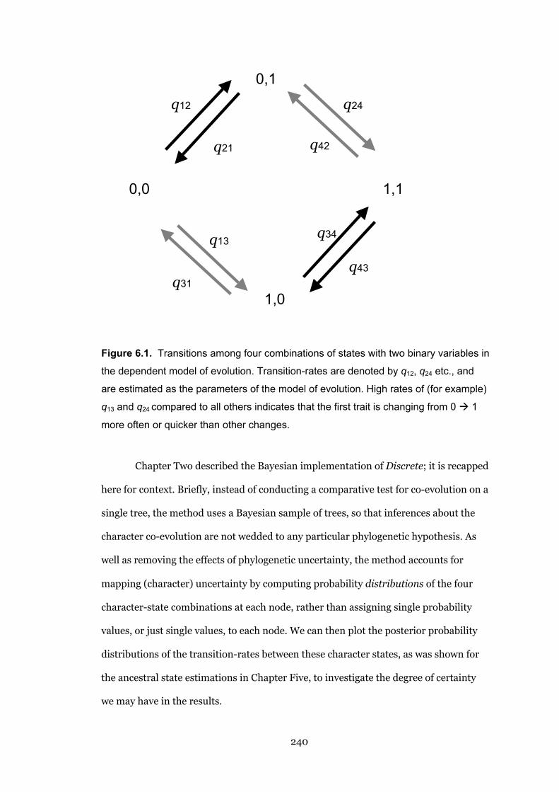
240
Figure 6.1. Transitions among four combinations of states with two binary variables in
the dependent model of evolution. Transition-rates are denoted by q12, q24 etc., and
are estimated as the parameters of the model of evolution. High rates of (for example)
q13 and q24 compared to all others indicates that the first trait is changing from 0 1
more often or quicker than other changes.
Chapter Two described the Bayesian implementation of Discrete; it is recapped
here for context. Briefly, instead of conducting a comparative test for co-evolution on a
single tree, the method uses a Bayesian sample of trees, so that inferences about the
character co-evolution are not wedded to any particular phylogenetic hypothesis. As
well as removing the effects of phylogenetic uncertainty, the method accounts for
mapping (character) uncertainty by computing probability distributions of the four
character-state combinations at each node, rather than assigning single probability
values, or just single values, to each node. We can then plot the posterior probability
distributions of the transition-rates between these character states, as was shown for
the ancestral state estimations in Chapter Five, to investigate the degree of certainty
we may have in the results.
1,0
1,1
0,1
0,0
q12
q21
q24
q13
q42
q34
q43q31
241
In the Bayesian context, we do not compare two single likelihoods to test the
independent versus dependent models, but rather we compare the two posterior
probability distributions of the likelihoods, in which there will be variation according
to the phylogenetic and trait uncertainty. We then ask a slightly different question:
which model, the dependent or the independent, accounts for a higher proportion of
the probability of the data? To do this we use the harmonic (marginal) means of the
likelihoods, derived at the convergence of the Markov chain run. We compute the
Bayes factor as BF = -2*(I-D), where a BF of 3–5 indicates positive evidence for the
dependent model, and greater than five indicates strong evidence (Pagel and Meade
2006). Harmonic means are sensitive to outliers and as such the analyses were run for
as long as possible to ensure that harmonic means were stable.
Markov chain. To run a co-evolutionary analysis, the program took two files,
(i) the tree-sample of 1000 phylogenies, and (ii) for each culture, information about
the state of the two traits presumed to be co-evolving. The independent and dependent
model parameters were estimated from a Markov chain that ran for 100 x 106
iterations, repeatedly visiting each tree in the sample of 1000. After convergence of the
chain, outcomes were sampled every 1000 iterations to avoid autocorrelation. This
provided 100,000 samples with which to estimate the marginal likelihoods, posterior
distributions and transition-rate parameters of the dependent and dependent models.
6.3.2.4 Using RJ MCMC to find the best models of evolutionary change
The transition rate parameters in Figure 6.1 give us a relative measure of which
transitions occur more often. BayesMultiState outputs these parameters, which we
then use to estimate the probable direction of evolution, that is, which trait changes
first in a possible evolutionary pathway. We are also able to determine the significance
of these changes using statistical tests. Previously, in the non-Bayesian (ML) version of
Discrete, the investigator proceeded by (arduously) setting each transition to zero, or
setting sets of transitions as equal, to see if this decreased the likelihood of the model
significantly; if it did, then that parameter was retained “as is” in the model of

242
evolution. If it did not alter the likelihood, then that switch was regarded as
unimportant in the co-evolutionary pathway. By reducing the number of transitions in
this manner, it was possible to compare the rate parameters and clarify which trait was
driving any co-evolutionary change, as Holden and Mace (2003) did in their analysis
of matriliny and cattle-keeping in Bantu-speaking societies.
The reversible-jump (RJ) MCMC procedure circumvents some of these aspects
of model-construction by using the Markov-chain device to explore the universe of
possible models, visiting them in proportion to their probability (Pagel and Meade
2006:809). In this context, a “model” is described as the set of eight transition-rate
parameters between the four states of character evolution, where transition-rates are
sorted into classes that are functionally equivalent. For example, the model
“1100000Z” denotes a situation where the transition rates of q12 and q13 are equivalent,
but different to all other rates in the flow diagram, except q43, which is
indistinguishable from zero. In the implementation of the RJ procedure, the program
reports the number of visits to each model in the sample. There are 21,147 possible
dependent models. Some number of these models will be equivalent to the
independent model (e.g. 00000000 or 11010100) because pairs of transitions will have
been assigned to the same rate class. The ratio of independent to dependent models in
the sample give an indication of whether correlated evolution is occurring. From
Stirling numbers (Pagel and Meade 2006) we expect a ratio of 413, that is, the
dependent model should be 413 times more prevalent in the sample than the
independent, i.e., the independent model should only account for 0.24% of those
present. If the chain visits independent models less than this, we have evidence for
correlated evolution. Ideally, only a small number of models will account for the
majority of the sample, indicating that other visited models are “noise” that may be
disregarded. Unlikely models may be visited a few times, but we are interested in those
that are repeatedly visited.
243
6.3.2.5 Hypothesis testing
In order to understand the most probable evolutionary pathways in the flow diagram,
we can (i) investigate the most commonly-visited model and (ii) select those models
which fit our hypothesis and compare their likelihoods (using the Bayes factor) against
those which do not. Comparing the dependent and independent models is the most
general form of this approach. For a more particular example, we might obtain
transition-rate parameters that indicate that the transition q13 is 100, compared to q12
which is 10. We wish to test if q13 > q12 is statistically significant, that is, whether q13 is a
“faster” rate and thus more likely to change first. To do this, we isolate those models in
which q13 is greater than q12, and note the harmonic mean of their marginal likelihoods.
These are then compared to the sample harmonic mean of marginal likelihoods of the
rest of our sample in the standard Bayes factor equation and the significance of the test
is thus judged from the outcome. Because harmonic means are sensitive to extreme
values, we compare only equal-size samples.
6.3.2.6 Using kappa to estimate the mode of character evolution
Kappa is a parameter that tests for punctuational versus gradual evolution by altering
the length of individual branches. κ = 0 indicates a star phylogeny when applied to
tree-building, or a punctuational mode of evolution when considering the evolution of
characters on a phylogeny (Freckleton et al. 2002). Kappa > 1.0 indicates that there is
more evolution on long branches (i.e., it stretches these more than short ones), while
values of κ < 1.0 indicate more evolution on shorter branches and thus compresses
longer ones. As well as being informative in its own right, κ can be estimated from the
data and then added to the model to improve the fit. I report κ values for all analyses.

244
6.3.3 Results
6.3.3.1 Phylogeny
The standard consensus phylogeny labelled with trait data is presented for the
unilineal/unilocal coding in Figure 6.2, and for the patrilineal/patrilocal coding in
Figure 6.3, overleaf. Both phylogenies show that more societies have the unilocal form
of residence than the unilineal form of descent. Figure 6.2 also has the ancestral states
of unilineal/unilocal traits mapped onto the early nodes of the trees. For this coding,
the program estimated the root to be unilocal (P(UR) = .71) and non-unilineal
(P(ND) = .77) under the independent model, and similarly (P(UR, ND) = .44) under the
dependent model. For the patri-coding, the estimates were less certain, with the root
equivocally patrilocal (P(PR) = .50) and non-patrilineal (P(OD) = .60) under the
independent model, and the same (P(PR, OD) = .57) under the dependent model.
6.3.3.2 Chi-square tests
A chi-square test (2 x 2 with 1 d.f.) for the unilineal coding was not significant
(χ2= 2.80, p ≤ .10). For the patri- coding there was a significant association as
χ2= 20.53, p ≤ .001.
6.3.3.3 Kappa
For the unilineal-coded analyses, kappa was estimated and found to have a mean of .52
±.15, with estimates ranging from .00 to 1.06. As this was a departure from the default,
implying a moderately punctuational mode of evolution, this parameter was
incorporated into subsequent co-evolutionary analyses. For the patri-coded analyses,
kappa was estimated using the independent model and found to have a mean of 1.06
±.22. As this was hardly different from the program default (κ = 1), it was left
unchanged in further analyses. However, estimates of kappa ranged from .00 to 1.62
(Figure 6.4), indicating that this parameter varied with different topologies and/or
models of evolution.
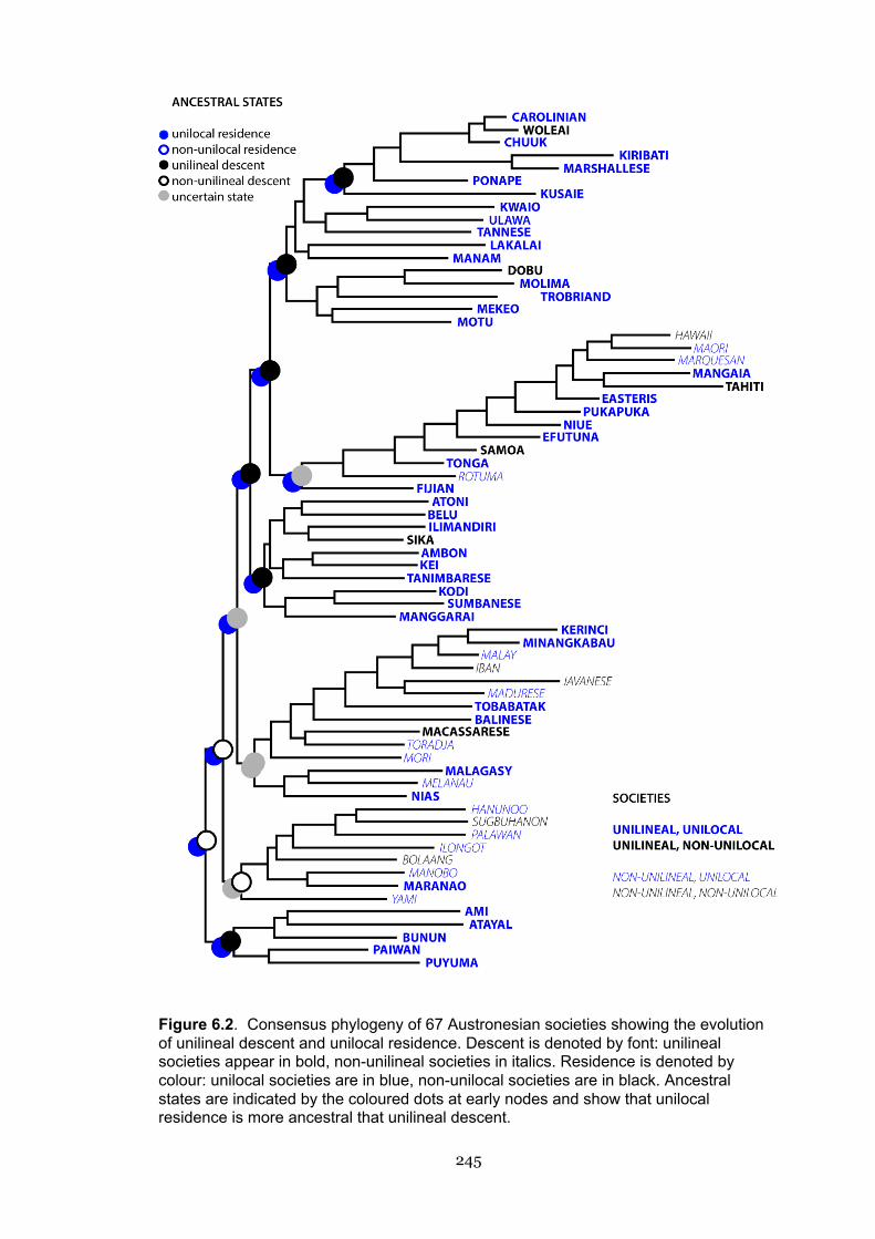
245
Figure 6.2. Consensus phylogeny of 67 Austronesian societies showing the evolutionof unilineal descent and unilocal residence. Descent is denoted by font: unilinealsocieties appear in bold, non-unilineal societies in italics. Residence is denoted bycolour: unilocal societies are in blue, non-unilocal societies are in black. Ancestralstates are indicated by the coloured dots at early nodes and show that unilocalresidence is more ancestral that unilineal descent.
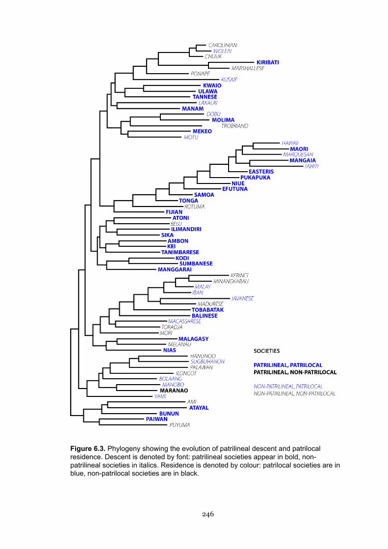
246
Figure 6.3. Phylogeny showing the evolution of patrilineal descent and patrilocalresidence. Descent is denoted by font: patrilineal societies appear in bold, non-patrilineal societies in italics. Residence is denoted by colour: patrilocal societies are inblue, non-patrilocal societies are in black.

247
Figure 6.4. Distribution of estimated kappa values for patri-coding. Low kappa values
indicate a punctuational mode of evolution, values around one indicate a gradualist
mode with change proportionate to branch length, while kappa values larger than one
indicate more change on longer branches. As the majority of values (87%) exceed .90,
we may conclude that these traits are evolving according to the phylogeny, i.e. they
are not following a punctuational mode.
6.3.3.4 Tests for co-evolution
For the unilineal coding, the mean marginal likelihood of the independent model,
using the harmonic mean, was –71.68, while that of the dependent model was –68.22.
Using the Bayes factor calculation, –2*(I–D), BF = 6.91, indicating that the hypothesis
of correlated evolution between descent and residence was positively supported.
Similarly, for the patri-coded data, there was strong positive evidence for the co-
evolution of the two traits (BF = 21.44).
The RJ MCMC procedure can also test if the hypothesis of correlated evolution
is supported by the data without using the Bayes factor. For each of the 100,000
samples, the program tells us if the model string found corresponds to an independent

248
or dependent model. Recall that the dependent model should be present 413 times
more than the independent for correlated evolution, i.e., the independent model
should represent 0.24% or less of the sample. For the unilineal coding, the
independent model accounted for (exactly) 0.24% of samples, and for the patri-coding,
the independent model only accounted for 0.002%. This is extra confirmation that the
co-evolutionary, dependent model fits these data better than the independent model.
We can probe further into the probable evolutionary pathway by examining the
transition-rate parameters. Descriptions of these evolutionary transitions are given in
Table 6.2. Flow diagrams (Pagel 1997) of evolutionary change are shown in Figures 6.5
and 6.6. For testing the hypothesis of co-evolution between descent and residence, we
are interested in the rates of q13, q31, q24, and q42, where a change in residence occurs
before a change in descent, and especially q13 and q24, where the transition occurs
towards lineality in social organisation.
Table 6.2. Description of the rate coefficients as applied to residence/descent data.
These descriptions can apply equally to the patri- coded data (Figure 6.5). The two
transitions in italics denote pathways towards lineal descent and residence where
residence changes first.
Coefficent Evolutionary transition
Gains
q12 Gain of unilinear descent system in the presence of non-unilocal residence
q13 Gain of unilocal residence in the presence of non-unilinear descent system
q24 Gain of unilocal residence in the presence of unilinear descent system
q34 Gain of unilinear descent system in the presence of unilocal residence
Losses
q21 Loss of unilinear descent system in the presence of non-unilocal residence
q31 Loss of unilocal residence in the presence of non-unilinear descent system
q42 Loss of unilocal residence in the presence of unilinear descent system
q43 Loss of unilinear descent system in the presence of unilocal residence
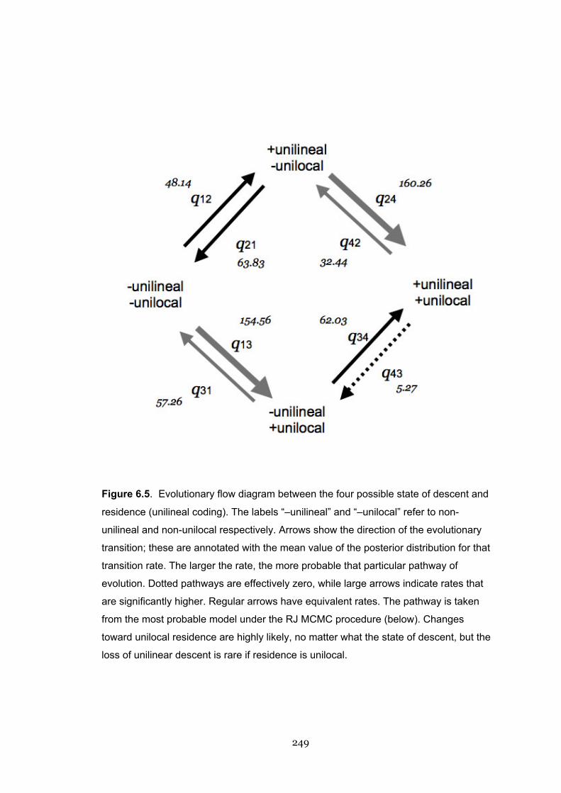
249
Figure 6.5. Evolutionary flow diagram between the four possible state of descent and
residence (unilineal coding). The labels “–unilineal” and “–unilocal” refer to non-
unilineal and non-unilocal respectively. Arrows show the direction of the evolutionary
transition; these are annotated with the mean value of the posterior distribution for that
transition rate. The larger the rate, the more probable that particular pathway of
evolution. Dotted pathways are effectively zero, while large arrows indicate rates that
are significantly higher. Regular arrows have equivalent rates. The pathway is taken
from the most probable model under the RJ MCMC procedure (below). Changes
toward unilocal residence are highly likely, no matter what the state of descent, but the
loss of unilinear descent is rare if residence is unilocal.

250
Figure 6.6. Evolutionary flow diagram between the four possible state of descent and
residence (patri- coding). The labels “–patrilineal” and “–patrilocal” refer to non-
patrilineal and non-patrilocal respectively. Arrows show the direction of the
evolutionary transition; these are annotated with the mean value of the posterior
distribution for that transition rate. The larger the rate, the more probable that particular
pathway of evolution. Dotted pathways are effectively zero, while large arrows indicate
rates that are significantly higher. Regular arrows have equivalent rates. The pathway
is taken from the most probable model under the RJ MCMC procedure (below).
Changes in residence are all likely, especially before descent, and when a society is
not patrilineal. However, once a society is both patrilineal and patrilocal residence is
unlikely to change.

251
Figure 6.7. Posterior distribution of the log-likelihoods of the independent and
dependent model for unilineal coding. Although they are only a few log-units apart the
distributions are clearly separated, indicating that the independent and dependent
models are occupying very different areas of parameter-space.
Testing the directionality of change. Figure 6.8 shows the posterior distributions
of the rate parameters under the dependent model for unilineal coding. We know that
the data support a hypothesis of correlated evolution, but we wish to determine the
model that describes the direction of evolutionary change. Examining the plots in
Figure 6.8, we see that the transitions where residence changes first have less of their
samples in the “zero bin”. Comparing q13 (residence first) and q12 (descent first), we
note that q13 has a wide distribution of rates, virtually all greater than zero and with a
mean of 160, while q12 has a majority of rate coefficients in the zero bin. The same
pattern holds for q42 (residence first) and q43 (descent first).
The output of the RJ MCMC procedure gives us “model strings” which sort the
transition-rates into classes, some of which may be the zero bin. Tables 6.3 and 6.4
show the most frequent models for both the unilineal and patri- coding.

252
Figure 6.8. Posterior distributions of the rate coefficients for unilineal descent and
unilocal residence under the dependent model of evolution. Plots are arranged so that
each row contains a pairs of rates that must be equal for the independent model to be
true (e.g. q12, q34), that is, the rates refer to the same evolutionary change in one trait
irrespective of the state in the other trait. There are differences between the first, third,
and fourth pairs in both the shape of the distribution and the number of time the rate is
at zero.

253
Table 6.3. Unilineal/unilocal data showing the seven most frequent models found by
RJ MCMC model-search, accounting for 55% of all the 10,000 samples. All models
have two parameters, meaning they are versions of the dependent model. The flow
diagram in Figure 6.5 is presented according to the most-frequent model.
Model string Frequency Cumulative frequency No. of parameters
0101000Z 1651 0.17 2
Z010111Z 1504 0.32 2
0000111Z 651 0.38 2
0101100Z 348 0.42 2
Z000101Z 339 0.45 2
Z0Z01011 331 0.48 2
0010111Z 323 0.51 2
The first two models, which account for nearly one-third of the sample, are equivalent
except for one difference, that of the transition q12 (gaining unilineal descent before
unilocal residence) being in the zero bin as well as q43. A large number of models have
the parameter q43 set to zero, indicating this transition (retaining unilocal residence
while losing unilineal descent) to be very unlikely. Taken together, these two
transitions being frequently set to zero is strong evidence that residence is changing
first for these data.
Table 6.4. Patrilineal/patrilocal data showing the eight most frequent models found by
RJ MCMC model-search, accounting for 48% of all samples. Only the third most-
frequent model has one parameter, equivalent to the independent model. All others
are a version of the dependent model. The flow diagram is presented according the
most-frequent model.
Model string Frequency Cumulative frequency No. of parameters
011110Z0 9384 0.093841 2
Z00100Z1 7483 0.168672 2
Z00000Z0 5982 0.228492 1
Z00Z00Z1 5960 0.288093 2
Z00000Z1 5762 0.345713 2
010110Z0 5609 0.401804 2
011111Z0 5285 0.454655 2
01Z110Z0 2958 0.484235 2

254
For the patri-coding, the q42 parameter (representing the loss of patriliny while
retaining patrilocality) is always in the zero bin, meaning that this transition is
effectively zero. The q12 parameter, where patriliny is gained before patrilocality, is also
frequently in the zero bin or in a lower rate class than other transitions. Models where
the parameters indicate that residence changes first or at a higher rate dominate the
sample.
We calculate if the models presented in the flow diagram are significant by
comparing the marginal means of those likelihoods to the likelihoods of an equal-sized
sample of all other models. For the unilineal coding, the flow-diagram model is
significant, as the likelihood was –62.38, compared to all other models whose mean
likelihood was –65.30, giving BF = 5.84. This is positive evidence in support of the
flow-diagram model. For the patri- coding, the flow diagram model likelihood was
–68.73 and that of all other models was –70.53, giving a BF = 3.6, which is moderate
evidence for the flow-diagram model. Thus, for both sets of coding, models in which
residence is likely to change first and/or changes in descent are less likely were
statistically supported by the data.
Calculating the posterior to prior odds. One final way of interrogating
the data to determine if a transition rate is significant is by calculating the posterior to
prior odds (M. Pagel, personal communication). To do this we use the full range of the
output and here test the proposition that q13 > q12, that is, that unilocal residence is
gained before unilineal descent. We can calculate the prior odds by examining the list
of all possible models (n = 21,147). First we remove those models in which q13 = q12
(leaving 17,000), and then isolate those models in which q13 > q12 (n = 7,000). Thus, we
expect .4 of the models (7,000/17,000) to support the hypothesis a priori. Then, we
use the Bayesian theorem to calculate the following (21,147 - 0.6*21,147) / (0.6*21,147)
where .6 is the proportion of models that cannot support the hypothesis (Lewis 2001).
The prior odds are thus (1 – 0.6)/0.6 = 0.666.

255
We then compare these prior (expected) odds to the observed data. We find
that the proportion of the observed sample that supports our hypothesis is .79, and the
proportion that does not support the hypothesis is .21. Using the Bayesian theorem,
the posterior odds are 10,000*(1 – .21)/.21*10,000 where 10,000 is the sample size,
giving 3.76. The Bayes factor is then 3.76/.66, BF = 5.65, supporting the hypothesis
that q13 > q12.
6.3.3.5 Rates of change over time
Finally, we can examine the rate of cultural evolution in descent and residence by
using the time scale of the Austronesian language tree to estimate the probability of a
change happening over a certain number of years. To do this we first derive an
approximate date for the root of the AN tree. The combination of archaeology and
linguistic evidence for the Austronesian expansion suggests that pottery-making
and/or agriculturalist peoples had moved from Taiwan to the Northern Philippines by
at least 5500 BP and to parts of Borneo by 4500 BP (Blust 1995; Bellwood 1998).
Evidence for an earlier start to the spread of Austronesian-speaking peoples has not
been forthcoming, so we may date Proto Austronesian to c.6000 BP, i.e. the tree
“length” from root to tips is 6000 years.
Taking the simplifying assumption that language change is proportionate to
time, we derive the length of the root-to-tip distances for each of the 67 societies and
average these to gain a measure of language change per year. TipToRoot, a program to
find these distances, was written for this purpose by A. Meade (personal
communication). The average tip-to-root distance was .04, meaning there was a 4%
change that the character state would change over the branch. As there were 17474
lexical characters, this meant that on average 698 characters changed from the root to
the tip. We use the following equation (Pagel and Meade 2005) to approximate the
probability of change from 01 on a branch of length t:
P(01)t = (α/(α + β))*(1 – e–(α+β)t) [Eq. 3]

256
where α and β are the transition-rate parameters between two states. Plugging the
transition rates for the dependent model of unilineal/unilocal evolution into Equation
3, we obtain the probability of change over different time periods (branch lengths),
shown in Table 6.5 and Figure 6.9.
Table 6.5. Probability of change in descent (top four parameters) and residence
(bottom four parameters) over three time periods. Parameters are taken from the
dependent model of evolution, as residence and descent show correlated evolution.
Evolutionary transition Probability of change over x years
100 1000 6000
q12 Gain unilineal descent without unilocal residence .03 .23 .43
q21 Lose unilineal descent without unilocal residence .04 .30 .56
q34 Gain unilineal descent with unilocal residence .04 .33 .86
q43 Lose unilineal descent with unilocal residence .00 .03 .07
q13 Gain unilocal residence without unilineal descent .09 .55 .73
q31 Gain unilocal residence without unilineal descent .04 .20 .27
q24 Gain unilocal residence with unilineal descent .10 .59 .79
q42 Lose unilocal residence with unilineal descent .03 .15 .21
Plotting the rates for residence and descent (Figure 6.9) shows that while there are
only small probabilities of change in both traits over 100 years, over the 1000-year
period the traits diverge. Residence is more labile, with a 15–59% chance of change
over 1000 years, compared to descent at 3–33%. Gains of unilocality have the highest
probability in a 1000-year period. Over the whole Austronesian tree, with a time
period of roughly 6000 years, the highest probability of all is the gain of unilineal
descent against a background of unilocal residence, indicating this is a stable state.

257
Figure 6.9. Probability of change over time in each of eight transitions according to
the dependent model. Dotted lines indicate changes in descent, solid lines indicate
changes in residence. There is a ~10% chance of change in both types of traits in the
100-year period. Changes to unilineal and –local forms are most probable over 1000
years, especially in residence, where there is a one in two chance of change. By 6000
years the traits have reached an equilibrium (i.e. probabilities add to one).

258
6.3.4 Discussion
Using a Bayesian MCMC procedure that controlled for phylogenetic uncertainty, I
found that changes in post-marital residence preceded changes in descent in 67
Austronesian societies, supporting the “main sequence” theory of kinship. This
relationship held true when the data was coded to reflect unilineal/-local versus non-
unilineal/-local kinship, and when coded to separate patrilineal/-local kinship from
other forms. Relating the changes to archaeological time, both traits had a low
probability of change over 100 years, but in a 1000-year period, residence had a 50%
likelihood of changing form.
6.3.4.1 Scenarios for the evolution of Austronesian unilocal and unilineal forms
Ancestral states for the AN tree, estimated in Chapter Five, give us the “start point” for
the evolutionary pathways that are presented in the flow diagrams. The most-likely
scenario for the evolution of unilineal descent and unilocal residence reconstructs the
root as non-unilineal (bilateral) but unilocal (possibly matrilocal, from Table 5.5). The
most common transition from this state is gaining unilineal descent, as in, for
example, the Formosan and Central Malayo-Polynesian societies. However, many
WMP societies in the Philippines and Indonesia “lose” unilocal residence, and are
bilateral and multilocal (e.g. Hanunoo, Balinese). One likely scenario for this transition
is that brideprice moderates residence in the poorer strata of many Island Southeast
Asian societies, for example, the Atoni of Timor (Cunningham 1967). Instead of paying
a brideprice, or as well as, the husband will live with the bride’s family for some period
of brideservice, creating a non-unilocal residence system. Considerations of brideprice
may also affect affiliation to one lineage or another in ambilineal cultures (Bellwood
1997). Indian and Islamic influences throughout Island Southeast Asia, from around
1000 BP (LeBar 1975; Denoon 1992) may also be a factor in the number of non-
unilineal systems in this area, although their effects on peasant classes (until recently
for Islam) are not well known (Alkire 1972). As well, many societies traditionally

259
practised shifting cultivation and had no shortage of land, a condition likely to favour
bilateral kinship e.g. the Iban of Borneo (Freeman 1981).
Unilineal descent evolves in the Proto Central-Eastern/Proto Oceanic part of
the tree, and once gained in the Oceanic group, only a few Polynesian societies revert
to a wholly non-unilineal form of descent, such as Hawai’i with bilateral descent
groups (Kirch 1984). Many Oceanic societies are ambilineal or have double descent, so
that both matri- and patri-lineal kin groups are present. By coding ambilineal societies
as unilineal, we capture the presence of lineal descent groups—the “unbroken line”
(Holy 1996)—in a society’s kinship structure, but we lose the aspect of flexibility in
social organisation that ambilineal societies share with cognatic and bilateral systems.
This flexibility may be important in explaining the predominance of ambilineal and
multilocal societies in Remote Oceania (Firth 1957; Fox 1967).
Non-unilineal systems. By allowing the individual some degree of choice in
their alignment with specific groups of kin, or permitting membership in multiple
types of kin groups, the apparent popularity of non-unilinear kin groups on small
islands may be a response to population pressure on a small area of land (Fox 1967).
Goodenough (1955) suggests that a number of social devices for the redistribution of
under-abundant land exist in Austronesian societies, chief amongst these being non-
unilinear kinship groups. When land was in abundance or the ecological environment
was predictable, tendencies towards unilinear descent could develop (1955:147). Eggan
(1966), examining North American societies, argued that buffalo-hunting societies
demonstrated a flexible social organisation that included multilocality and cognatic
descent, in response to the seasonal and precarious nature of their subsistence.
Is non-unilineal descent (and multilocal residence) adaptive for societies that
face environmental risk? It may be the case that cognatic/ambilineal descent reflects
an adjustment to fluctuating or marginal environments. The dangers of long distance
voyaging and depopulation during migration have also been suggested as possible
factors encouraging the development of non-unilineal descent in Oceania (Lane 1961).
260
Some authors (Forde 1947; Lee 1972) have noted that residential flexibility is adaptive
when resources are unpredictable. If, as the results presented here suggest, Murdock’s
theory of kinship change is correct, then further studies should assess if there is a
consistent correlation between environmental risk factors and non-unilineal social
organisation in Austronesian societies.
6.3.4.2 Patrilineal organisation in Austronesian societies
The ancestral states analyses in Chapter Five indicated that the root of the AN
tree was probably neither patrilineal nor patrilocal. Thus, the most likely evolutionary
scenario for these cultures is that patrilocality is rapidly gained and lost against the
background of a non-patrilocal descent system. Lessa (1950) describes the matrilineal
descent and patrilocal residence of Ulithi Atoll in Micronesia, remarking that bride-
service sometimes requires residence with the bride’s family. It is easy to see that in
conditions like these, residence patterns, as “cultural traits”, are more likely to be
decisions for the individual, and are likely to have high rates of change. According to
the flow diagram model, however, once patrilocality is gained, some further “push”
may be required to shift the kinship structure towards patriliny. In Austronesian
societies this push may be entwined with aspects of ranking, primogeniture, and status
(Bellwood 1996c; Kirch and Green 2001). So for instance, while the Kwaio of the
Solomon Islands have a bilateral/cognatic form of descent, patrilineally-affiliated
members have higher status (Keesing 1970), and conversely, in the cognatic hapu
systems of the New Zealand Maori, affiliation was traditionally preferentially to the
fathers’ line, except when the line of the mother had higher status (Scheffler 1964).
Once a society is both patrilineal and patrilocal it is unlikely to shift away from
this state. If it does, it will most certainly not shift to a different residence system first.
The only society in our sample that has patrilineal descent groups and non-patrilocal
residence is the Maranao of the Southern Philippines, who are matrilocal and neolocal.
However, their descent system is complex: “all persons inherit at least two descent
lines, some claim as many as fifteen” (Mednick 1975). Thus, Murdock’s assertion that
261
“although unilocal residence does not necessarily lead to unilinear descent ... unilinear
descent can arise in no other way than through unilocal residence” (1949:209) applies,
at least to patriliny.
Service (1962) observed that patrilocality occurs in so many different ecological
and cultural contexts that no clear patterns can emerge to explain its global
predominance. However, as evidenced by its prevalence worldwide (~70%, Levinson
and Malone 1980), patriliny may “stick” in many cases as it conforms to some basics of
evolutionary biology (Hartung 1976; Alexander 1979). That is, the greater reproductive
variance of males as opposed to females means that if resources are available to be
transferred, it makes more sense to invest them in males: “a daughter’s reproductive
success is less affected by poverty than a son’s” (van den Berghe 1979:96). On this
model, in those Austronesian societies where individuals may acquire heritable wealth,
patriliny may become common, as is the case in Bantu-speaking populations in Africa
(Mace 1996; Holden and Mace 2003). This may be the situation for the Manggarai of
Flores, in the “patrilineal” CMP clade, who keep buffalo and horses for prestige and for
brideprice payments. In this respect, however, they are unlike many Austronesian
societies (especially those in the Remote Pacific) who do not have large domestic
livestock or similar forms of transferable wealth.
Bellwood (1997) has tentatively suggested that contact with non-Austronesian
populations in eastern Indonesia and Melanesia may have provoked a shift towards
unilineal organisation. These NAN societies are predominantly unilineal, especially
patrilineal in the case of Papuan-speaking New Guinea societies (Brown 1978), and
may have influenced the Austronesian populations that travelled through and/or
settled in those areas (i.e. CMP and Oceanic groups) towards unilineal descent, while
those societies in western Island Southeast Asia remained, or developed non-unilineal
kinship. This suggestion, though speculative, does not conflict with the findings
presented here.

262
6.3.4.4 Rates of cultural evolution
By calibrating the language tree with archaeological estimates of the age of the
Austronesian language family, we were able to estimate rates of cultural evolution.
Two points are of note. First, different dynamics of change are at work over different
time periods. The probability of change to unilocal post-marital residence over a 1000-
year period was much more than the probability over 100 years, but was less than a
linear relationship with time would suggest. This indicates that there may be limits on
the rate of cultural change, or, that some form of equilibrium where societies can
switch their residence pattern back and forth is reached. Second, rates of cultural
change are not homogenous for all traits. For these societies, change to unilocal
residence had a much higher probability (and more variation) of change over the
1000-year period than did descent, indicating that of the two it may indeed be the
more labile trait. Goodenough (1956) found that residence patterns in Chuuk, as
recorded in census data, could fluctuate throughout a decade. We would expect this to
follow from the main sequence hypothesis, if it is the underlying conditions causing
residence change, rather than descent, which act first. In addition, Divale (1974)
estimated that some societies had unilocal residence for up to a thousand years
without developing a unilineal form of descent, so whatever benefits are to be gained
by unilocal residence, they do not necessarily cause an immediate transition to
unilineality. From an evolutionary perspective, localising one type of kin (male or
female) may have benefits that are not to do with inheritance of resources/material
wealth, but concern aspects of kin investment through childcare and time allocation.
6.3.4.5 Desirability of multi-state models
A more complex model of the transitions between descent and residence in
Austronesian societies remains to be constructed and tested. The primary drawback is
that we are effectively limited to a two-state test using binary coding, when ideally a
multi-state coding is preferred. Chapter Five revealed the difficulties in applying a
263
multi-state model to a data set of this size and “messy” cultural nature; it is difficult to
gain statistical significance when the variance must be partitioned in a combinatorial
arrangement of three states for two characters. Unfortunately, in the Austronesian
world there are real-world functional differences between bilateral, ambilineal, and
patri- or matri-lineal descent groups. Ambilineal societies occupy an uneasy space
between bilateral/cognatic and pure lineal systems, but the fact that they are prevalent
and pervasive in the Pacific is indication that they are a distinct form of kinship
organisation deserving of independent explanation. For example, Murdock (1949:205)
attributes the predominance of ambilocal systems in Polynesia to the importance of
senior-junior ranking and primogeniture, as opposed to differentiation by sex, because
the higher-status (first-born) spouse will often remain with the natal family regardless
of sex. In another vein, Service (1962) had suggested that depopulation events should
trigger a shift from unilocal to ambilocal residence as groups sought to re-establish
control of resources by a flexible attitude towards social organisation. In addition, C.
Ember (1974) found that hunter-gatherer ambilocalism was predicted by a
depopulation event (at least a 25 percent decrease) in the 30 years prior to the
ethnographic present. In the Pacific context, a migration event could be seen as
equivalent to depopulation, and thus may account for the large number of ambilocal
societies seen in the Pacific.
Understanding the relationships between bilateral, ambi-, matri-, and patri-
lineal descent, and different forms of residence, will require careful tests that unpack
functional and/or causal relationships. Testing the main sequence was the very
beginning of this process, but clearly demonstrated the necessity of a phylogenetic
comparative approach to testing these anthropological “truisms”.

264
6.4 Is matriliny co-evolving with male absence?
6.4.1 Introduction
Burton et al. (1996), analyzing worldwide trends in social structure through
correspondence analysis, characterised the Southeast Asia and the insular Pacific as a
“matricentric” region, one that organised “kinship groups around women through
matrilocal or uxorilocal residence or through matrilineal kinship groups” (1996:93).
Matrilineal descent and matrilocal residence are found at a higher frequency in the
Austronesian societies of the Ethnographic Atlas than the overall worldwide average
(see Table 5.1). In matrilineal societies, inheritance of property and political title are
usually passed from mother’s brother to sister’s son (Gaulin and Schlegel 1980), as in
the Trobriand Islanders (Weiner 1978), or from mother to daughter, as in the
Minangkabau (Kahn 1980; Sanday 2002). Matriliny presents a “puzzle” (Richards
1950) because kinship is organised around women, yet men remain politically and
socially dominant. Pursuing the solution to the matrilineal puzzle has provoked
anthropologists into proposing a number of explanatory hypotheses.
Cross-culturally, matriliny has been associated with a horticultural mode of
production (Murdock 1949; Aberle 1961). In the African Bantu language family,
Holden and Mace (2003) used phylogenetic comparative methods to demonstrate that
the adoption of domestic livestock as a subsistence practice led to the loss of matriliny.
Cultures that possessed cattle were more likely to be patrilineal or have double
descent. In an evolutionary context, the acquisition of cattle is the acquisition of
heritable/defendable wealth, which can then be passed (patrilineally) on to sons to
improve their chances of reproductive success. However, the majority of Austronesian
cultures do not have large herds of domestic livestock, and so this explanation is not
appropriate to the Pacific context. The general form, that heritable and transferable
wealth encourages patrilineal forms of social organisation, is also hard to apply in the
Austronesian context. Houses, land, and gardens are just as likely to be collectively
owned by a lineage or some other form of corporate descent group as by individuals;

265
membership in descent groups regulates access to resources, not ownership
(Crocombe 1974; Ward 1997).
High paternity uncertainty has long been associated with the matrilineal
transmission of wealth to sisters’ sons (Morgan 1877), as maternity certainty ensures a
man of his relationship to his sister and her offspring. Hartung (1981, 1985) proposed
a model in which only small amounts of paternity uncertainty are necessary for
matrilineal inheritance to be adaptive over a few generations, and reviewed cross-
cultural evidence to suggest that matrilineal societies were often those with moderate
to low certainty of paternity. The causal arrow could, however, go both ways, and
factors which may promote paternity uncertainty are of interest in this instance.
Using data from Otterbein and Otterbein (1965), Ember and Ember (1972)
proposed a model in which the nature of warfare experienced by societies moderated
the effect of the sexual division of labour (SDL) on residence. Simply, the presence of
internal warfare (i.e. fighting between intermarrying communities) favours patrilocal
residence, as matrilocal residence causes a conflict of interest for men between their
natal and their wives’ community. Ember and Ember found that a significant
association between SDL and residence only holds when only external warfare is
present, remarking that “if the males have to be away often on long trading trips (as in
parts of Micronesia and Melanesia in the recent past) … and work has to be done while
they are away, the women might end up doing at least as much as the men in
subsistence activities, even though warfare is no longer present” (1972:581).
Harris (1985) made the general argument that matrilineality is favoured under
conditions when there is prolonged male absence—and by extension, high male
mortality. In Harris’s view, the lineage interests of absent brothers (due to warfare,
trade, voyaging, or resource exploitation) are best managed by their sisters, who have a
familial interest, rather than by unrelated wives. Matri-dominant social organisation in
the Caribbean and West Indies was seen, in a similar vein, to be a response compelled
by absent (warfaring or seafaring) husbands (Keegan and Maclachan 1989). Levi-

266
Strauss (1984) observed that in Micronesia, a matrilineal form of social organisation
meant that males were easily assimilated, a probable necessity for a seafaring
population where male mortality might be high (Keegan 1989). We may re-cast these
arguments in terms of resource allocation and inclusive fitness by considering how
maternal grandparents might wish to invest their resources in their grandchildren, as
Hartung (1985:684) wondered:
“In the face of high rates of mortality for males in their reproductiveprime, matrilineality may have been a more fundamental form of socialsecurity than has since been invented.”
Hage and Marck (2003) also associate the continuation of regular long-distance
voyaging in Micronesia with that area’s matrilineal kin groups. Moreover, Aberle
(1961) found that although horticultural production was the predominant mode of
susbistence associated with matriliny (though not in Oceania), there was an
unexplained tendency for matriliny to be associated with fishing. He noted that:
“The logical possibility exists that the connection between matrilinealityand horticulture is accidental, and that the crucial issue is the amountof fishing or the kind of fishing done.” (Aberle 1961:703)
Thus, the “absence of males” or high male mortality in the Austronesian context might
be due to dependence on fishing, warfare, or voyaging/trade. Each of these provides a
comparative hypothesis for testing in a phylogenetic framework. In addition, the
absence of males may be a reason for low paternity certainty, if we can invoke
Hartung’s hypothesis. Here I concentrate on the association of matriliny and fishing.
Although the relationship has been noted in the literature, it has not been tested in a
quantitative manner by either traditional cross-cultural association tests or
phylogenetic methods, affording a novel opportunity to statistically assess an untested
anthropological proposition.

267
6.4.1.1 Hypotheses
Here I test the hypothesis of correlated evolution between matrilineal social
organisation and an aspect of “male absence”, namely a high degree of dependence on
male fishing for subsistence. In the Austronesian/Pacific context, this may be the most
appropriate single measure to quantify “male absence”, due to the large number of
oceanic/island societies. As well, quantitative data on the dependence of fishing, as
well as information on the sexual division of labour, are available for many of these
societies in the EA (Murdock 1967). Secondly, I test whether matriliny and high fishing
dependence (and/or the absence of both) represent “evolutionary stable strategies”
(Maynard Smith 1992) or stable states by testing if transitions towards those states
have higher likelihoods than other transitions.
6.4.2 Methods
6.4.2.1 Phylogeny estimation
The 67-language data set and the corresponding 1000-tree Bayesian sample, as
described in Chapter Two, were used for these analyses.
6.4.2.2 Cultural data and coding schemes
The ethnographic data on descent and residence compiled for Chapter Five were used
in these analyses (see Tables 5.2 and 5.4). Two tests were conducted, one using
matrilineal descent, the other using matrilocal residence. Societies were coded “MD” as
matrilineal in descent if they were matrilineal, ambilineal, or had double descent. All
others were non-matrilineal (“OD”). This corresponded to the “matrilineal aspect”
coding in Chapter Five. Societies were coded for matrilocality in residence (“MR”) if
they were matrilocal, avunculocal or ambilocal. All others were coded as non-
matrilocal (“OR”).

268
Data for dependence on fishing came from the three ethnographic sources used
in Chapter Five: the Ethnographic Atlas, plus the Ethnic Groups of Island South-east
Asia, and the Encyclopaedia of World Cultures. I used the EA codes for “dependence
on fishing” and “sexual division of labour for fishing”, supplementing this with
additional ethnographic descriptions in the other sources, to construct a binary coding
scheme for dependence on (male) fishing (Table 6.5). A society was coded “F” it had
“dependence on fishing” greater than 25 percent (or a high dependence was noted in
other sources), and an indication that men did appreciably more fishing than women
and at least some fishing was offshore (n = 30). Where information was available that
sea-voyaging trade was important, that society was also coded “F”. Societies not
meeting these criteria were coded “N” (n = 34). Three societies were coded as having
missing data due to insufficient information. Table 6.7 shows the contingency table for
the coded traits. Chi-square tests are reported in the results.
Table 6.6. Contingency table for matriliny and fishing showing the number of societies
classified in each trait class. Each of the cells corresponds to one of the four states in
the evolutionary “flow diagrams”.
Matrilineal (MD) Non-matrilineal (OD)
High dependence on male fishing (F) 44 12
Low dependence on male fishing (N) 6 5

Table 6.7. Information on fishing for 67 Austronesian societies.
ETHNOGRAPHIC ATLAS VARIABLES OTHER SOURCES1
Society Name Dependence2 Sex differences: fishing3 EWC EGI Code4
Ambon 26–35% Missing data Men fish, fishing important – F
Ami 6–15% Males only Fishing not remarked – N
Atayal 6–15% Males only Highland group, fishing by poison – N
Atoni – – Fishing not remarked Inland communities,
fishing not remarked
N
Balinese 0–5% Absent/unimportant Fishing not remarked – N
Belu 0–5% Missing data Fishing insignificant – N
Bolaang – – – Fishing present; coastal
village; supplemental
N
Bunun 0–5% Absent/unimportant Highland settlements Inland (riverine) N
Carolinian 46–55% Males only – – F
Chuuk 46–55% Differentiated but equal Men fish offshore, women fish on reef,
trade with other islands
– F
Dobu 26–35% Males appreciably more Men offshore on kula expeditions – F
Easter Is. 6–15% Males appreciably more Men fished, but not a major activity – N
E. Futuna 26–35% Females appreciably more Men fish coastally (offshore
dangerous), women reef
– F
Fijiian 46–55% Males appreciably more Men offshore, women reef, wide
trading networks by canoe
– F
Hanunoo 6–15% Males appreciably more Fishing important, mainly trapping– – N
269

Table 6.7 (Continued). Information on fishing for 67 Austronesian societies.
ETHNOGRAPHIC ATLAS VARIABLES OTHER SOURCES1
Society Name Dependence2 Sex differences: fishing3 EWC EGI Code4
Hawaii 36–45% Males appreciably more Men offshore, women reef,
occasional trading/voyaging
– F
Iban 16–25% Males appreciably more Riverine fishing, traditional raiding – N
Ili Mandiri 26–35% Missing data Men fish; whaling in Lamaholot – F
Ilongot – – Fish trapping Highland village, stream fishing N
Javanese 0–5% Absent/unimportant Fishing insignificant – N
Kei 16–25% Missing data Fishing important – -
Kerinci – – – Lake fishing, men fish F
Kiribati 46–55% Males appreciably more Men do most of the fishing, sea
voyaging/trading
– F
Kodi 0–5% Missing data – – N
Kusaie 36–45% Differentiated but equal Men use canoes – F
Kwaio 26–35% Missing data Men fish, tradition of elaborate
canoe building
– F
Lakalai 16–25% Differentiated but equal Men offshore, women stream – NMacassarese 16–25% Males only Men fish in coastal villages – N
Madurese – – Men fish by outrigger canoe and net Important for subsistence,
offshore fishing
F
Malagasy 6–15% Females appreciably more – – N
Malay 16–25% Males only Important depending on village – N
270
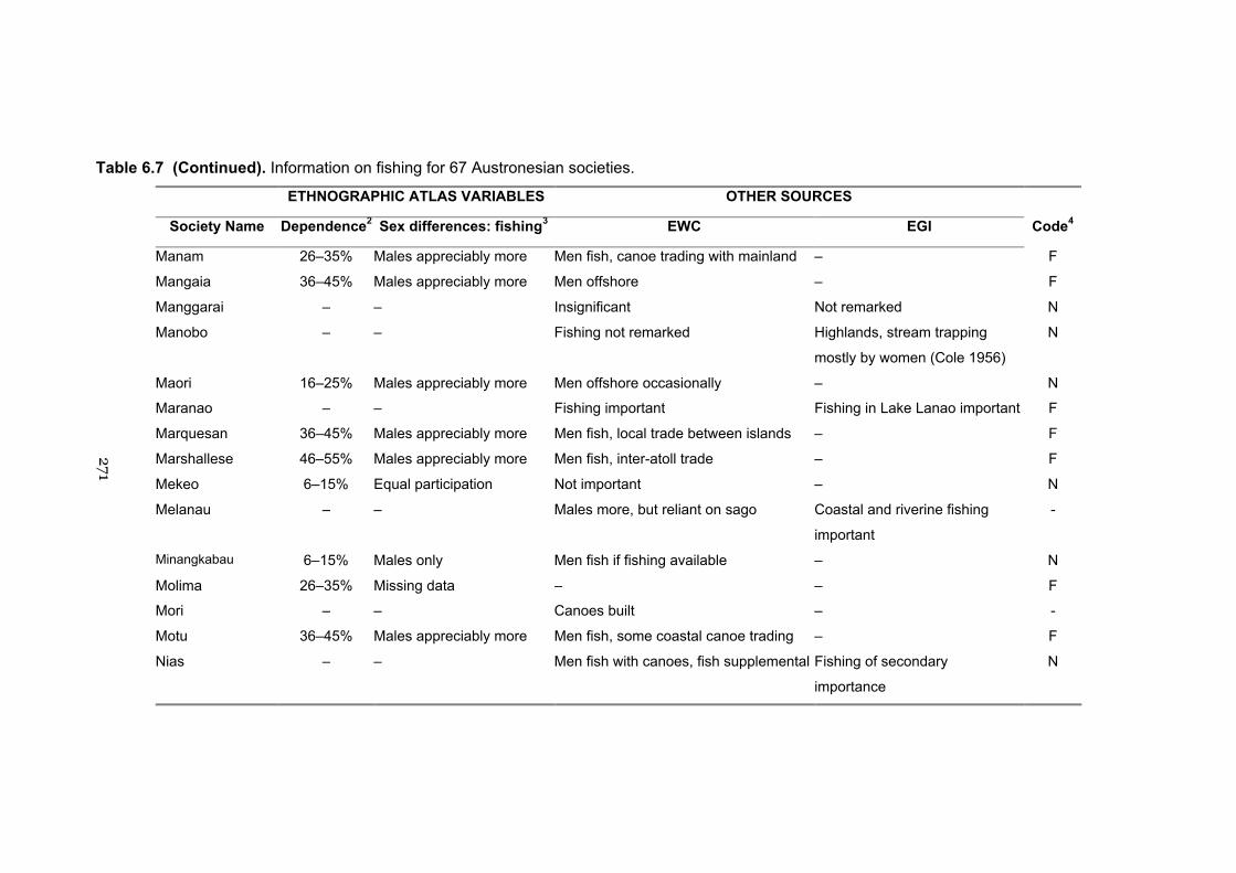
Table 6.7 (Continued). Information on fishing for 67 Austronesian societies.
ETHNOGRAPHIC ATLAS VARIABLES OTHER SOURCES
Society Name Dependence2 Sex differences: fishing3 EWC EGI Code4
Manam 26–35% Males appreciably more Men fish, canoe trading with mainland – F
Mangaia 36–45% Males appreciably more Men offshore – F
Manggarai – – Insignificant Not remarked N
Manobo – – Fishing not remarked Highlands, stream trapping
mostly by women (Cole 1956)
N
Maori 16–25% Males appreciably more Men offshore occasionally – N
Maranao – – Fishing important Fishing in Lake Lanao important F
Marquesan 36–45% Males appreciably more Men fish, local trade between islands – F
Marshallese 46–55% Males appreciably more Men fish, inter-atoll trade – F
Mekeo 6–15% Equal participation Not important – N
Melanau – – Males more, but reliant on sago Coastal and riverine fishing
important
-
Minangkabau 6–15% Males only Men fish if fishing available – N
Molima 26–35% Missing data – – F
Mori – – Canoes built – -
Motu 36–45% Males appreciably more Men fish, some coastal canoe trading – F
Nias – – Men fish with canoes, fish supplemental Fishing of secondary
importance
N
271
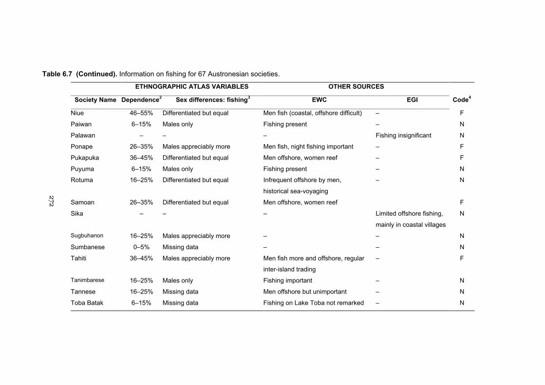
Table 6.7 (Continued). Information on fishing for 67 Austronesian societies.
ETHNOGRAPHIC ATLAS VARIABLES OTHER SOURCES
Society Name Dependence2 Sex differences: fishing3 EWC EGI Code4
Niue 46–55% Differentiated but equal Men fish (coastal, offshore difficult) – F
Paiwan 6–15% Males only Fishing present – N
Palawan – – – Fishing insignificant N
Ponape 26–35% Males appreciably more Men fish, night fishing important – F
Pukapuka 36–45% Differentiated but equal Men offshore, women reef – F
Puyuma 6–15% Males only Fishing present – N
Rotuma 16–25% Differentiated but equal Infrequent offshore by men,
historical sea-voyaging
– N
Samoan 26–35% Differentiated but equal Men offshore, women reef F
Sika – – – Limited offshore fishing,
mainly in coastal villages
N
Sugbuhanon 16–25% Males appreciably more – – N
Sumbanese 0–5% Missing data – – N
Tahiti 36–45% Males appreciably more Men fish more and offshore, regular
inter-island trading
– F
Tanimbarese 16–25% Males only Fishing important – N
Tannese 16–25% Missing data Men offshore but unimportant – N
Toba Batak 6–15% Missing data Fishing on Lake Toba not remarked – N
272
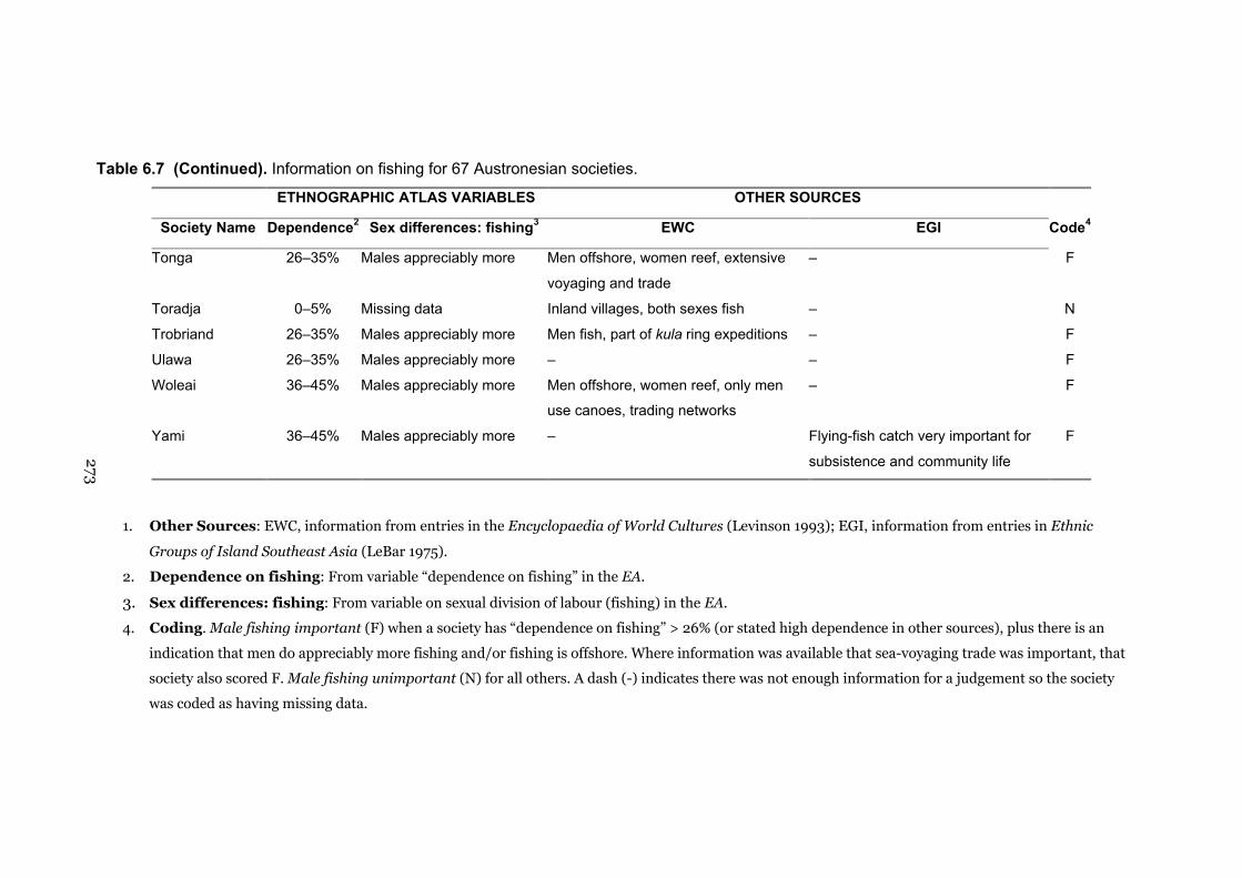
Table 6.7 (Continued). Information on fishing for 67 Austronesian societies.
ETHNOGRAPHIC ATLAS VARIABLES OTHER SOURCES
Society Name Dependence2 Sex differences: fishing3 EWC EGI Code4
Tonga 26–35% Males appreciably more Men offshore, women reef, extensive
voyaging and trade
– F
Toradja 0–5% Missing data Inland villages, both sexes fish – N
Trobriand 26–35% Males appreciably more Men fish, part of kula ring expeditions – F
Ulawa 26–35% Males appreciably more – – F
Woleai 36–45% Males appreciably more Men offshore, women reef, only men
use canoes, trading networks
– F
Yami 36–45% Males appreciably more – Flying-fish catch very important for
subsistence and community life
F
1. Other Sources: EWC, information from entries in the Encyclopaedia of World Cultures (Levinson 1993); EGI, information from entries in Ethnic
Groups of Island Southeast Asia (LeBar 1975).
2. Dependence on fishing: From variable “dependence on fishing” in the EA.
3. Sex differences: fishing: From variable on sexual division of labour (fishing) in the EA.
4. Coding. Male fishing important (F) when a society has “dependence on fishing” > 26% (or stated high dependence in other sources), plus there is an
indication that men do appreciably more fishing and/or fishing is offshore. Where information was available that sea-voyaging trade was important, that
society also scored F. Male fishing unimportant (N) for all others. A dash (-) indicates there was not enough information for a judgement so the society
was coded as having missing data.
273
274
6.4.2.3 Testing for correlated evolution
BayesMultiState was used in Discrete mode as described previously. The independent
and dependent model parameters were estimated from a Markov chain that ran for
500 x 106 iterations, repeatedly visiting each tree in the sample of 1000. After
convergence of the chain, outcomes were sampled every 10,000 iterations to avoid
autocorrelation. This provided 50,000 samples with which to estimate the marginal
likelihoods, posterior distributions and transition-rate parameters of the dependent
and dependent models. The proposal mechanism for the Markov chain was set to 20,
resulting in ~35% of proposed models being accepted as the next step in the chain. An
exponential distribution with a mean of 50 was used to constrain the values from
which the chain drew its prior probabilities, effectively constraining the wide
parameter space to be explored more thoroughly. Bayes factor tests using the marginal
means of the likelihoods were used to test hypotheses of (i) co-evolution and (ii)
identify which trait was changing first.
6.4.3 Results
6.4.3.1 Phylogenetic analysis
The phylogeny is shown in Figure 6.10 with cultural data on fishing and matrilineal
descent plotted for each society. The most probable ancestral states at the root of the
tree under the independent model are non-matrilineal descent, P(OD) = .98, and with
low dependence on male fishing, P(N) = .78. This finding concurs with the estimation
of the root as having non-matrilineal descent in Chapter Five. Under the dependent
model the highest estimate for the root is the same as for the independent P(OD,N) =
.62, followed by P(MD,N) = .27. This means that a quarter of the reconstructions show
a root that was already matrilineal.
The ancestral state at the root was equivocally matrilocal, P(MR) = .55. This
difference from estimates in Chapter Five may stem from the more strict definition of
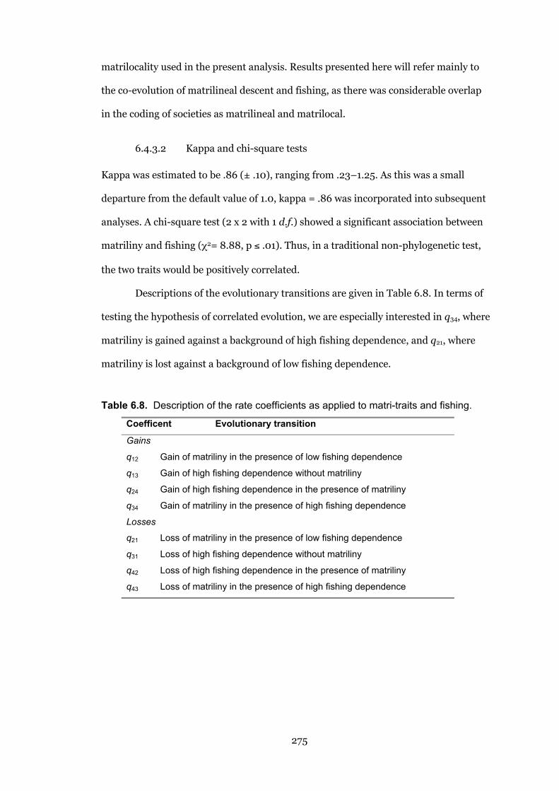
275
matrilocality used in the present analysis. Results presented here will refer mainly to
the co-evolution of matrilineal descent and fishing, as there was considerable overlap
in the coding of societies as matrilineal and matrilocal.
6.4.3.2 Kappa and chi-square tests
Kappa was estimated to be .86 (± .10), ranging from .23–1.25. As this was a small
departure from the default value of 1.0, kappa = .86 was incorporated into subsequent
analyses. A chi-square test (2 x 2 with 1 d.f.) showed a significant association between
matriliny and fishing (χ2= 8.88, p ≤ .01). Thus, in a traditional non-phylogenetic test,
the two traits would be positively correlated.
Descriptions of the evolutionary transitions are given in Table 6.8. In terms of
testing the hypothesis of correlated evolution, we are especially interested in q34, where
matriliny is gained against a background of high fishing dependence, and q21, where
matriliny is lost against a background of low fishing dependence.
Table 6.8. Description of the rate coefficients as applied to matri-traits and fishing.
Coefficent Evolutionary transition
Gains
q12 Gain of matriliny in the presence of low fishing dependence
q13 Gain of high fishing dependence without matriliny
q24 Gain of high fishing dependence in the presence of matriliny
q34 Gain of matriliny in the presence of high fishing dependence
Losses
q21 Loss of matriliny in the presence of low fishing dependence
q31 Loss of high fishing dependence without matriliny
q42 Loss of high fishing dependence in the presence of matriliny
q43 Loss of matriliny in the presence of high fishing dependence
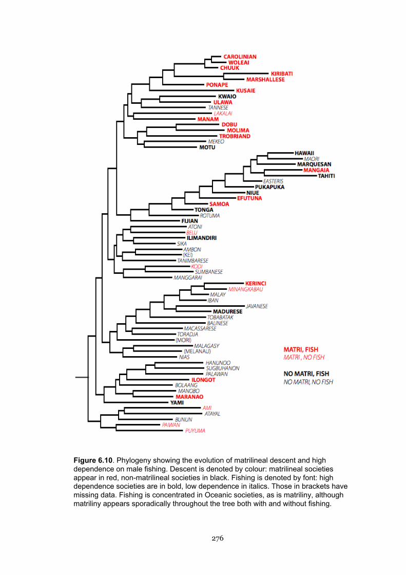
276
Figure 6.10. Phylogeny showing the evolution of matrilineal descent and highdependence on male fishing. Descent is denoted by colour: matrilineal societiesappear in red, non-matrilineal societies in black. Fishing is denoted by font: highdependence societies are in bold, low dependence in italics. Those in brackets havemissing data. Fishing is concentrated in Oceanic societies, as is matriliny, althoughmatriliny appears sporadically throughout the tree both with and without fishing.
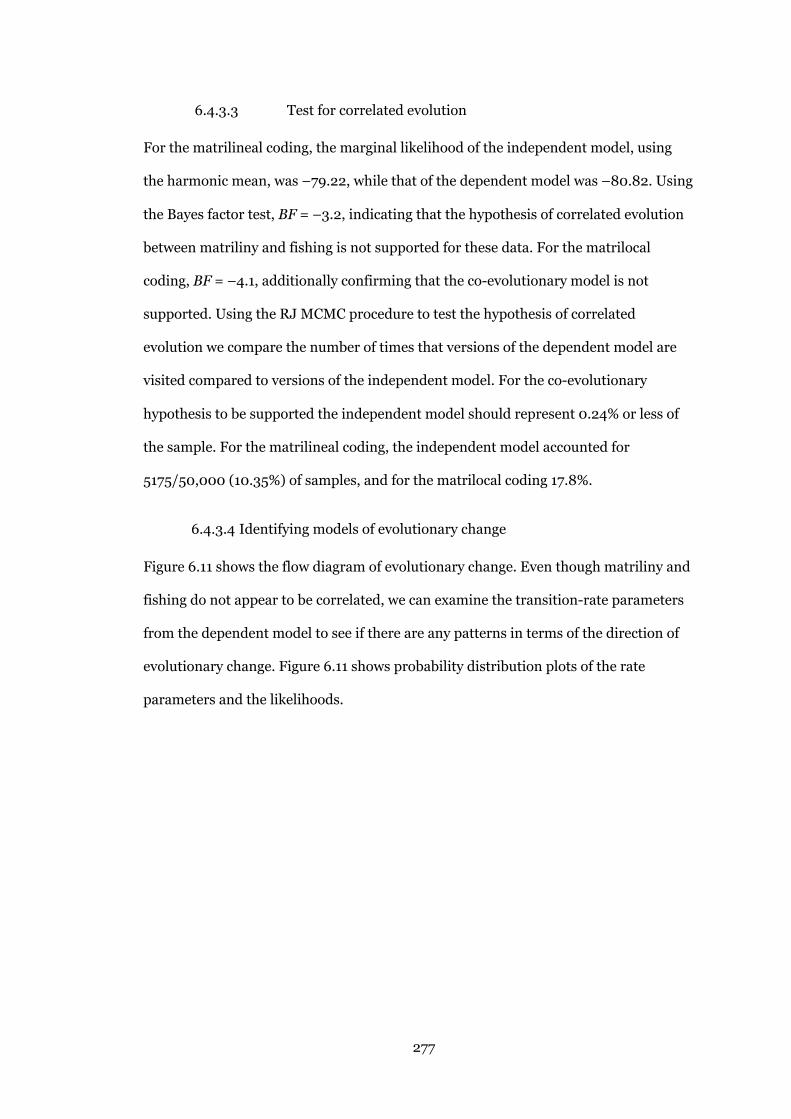
277
6.4.3.3 Test for correlated evolution
For the matrilineal coding, the marginal likelihood of the independent model, using
the harmonic mean, was –79.22, while that of the dependent model was –80.82. Using
the Bayes factor test, BF = –3.2, indicating that the hypothesis of correlated evolution
between matriliny and fishing is not supported for these data. For the matrilocal
coding, BF = –4.1, additionally confirming that the co-evolutionary model is not
supported. Using the RJ MCMC procedure to test the hypothesis of correlated
evolution we compare the number of times that versions of the dependent model are
visited compared to versions of the independent model. For the co-evolutionary
hypothesis to be supported the independent model should represent 0.24% or less of
the sample. For the matrilineal coding, the independent model accounted for
5175/50,000 (10.35%) of samples, and for the matrilocal coding 17.8%.
6.4.3.4 Identifying models of evolutionary change
Figure 6.11 shows the flow diagram of evolutionary change. Even though matriliny and
fishing do not appear to be correlated, we can examine the transition-rate parameters
from the dependent model to see if there are any patterns in terms of the direction of
evolutionary change. Figure 6.11 shows probability distribution plots of the rate
parameters and the likelihoods.
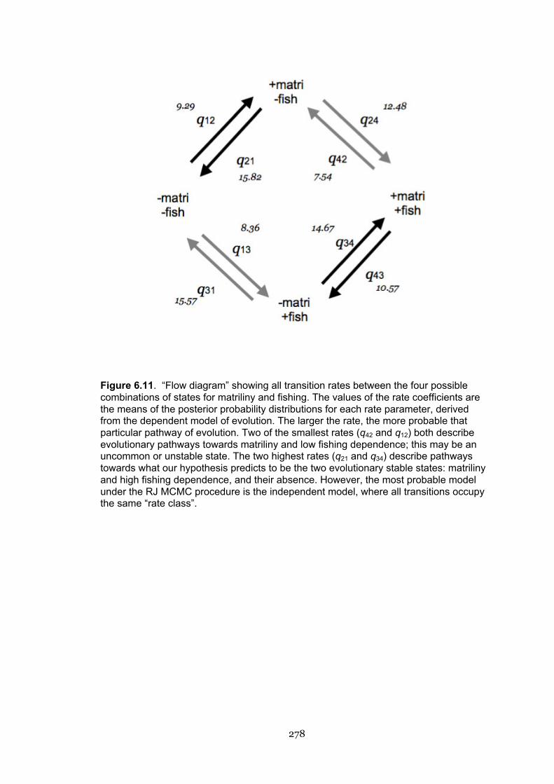
278
Figure 6.11. “Flow diagram” showing all transition rates between the four possiblecombinations of states for matriliny and fishing. The values of the rate coefficients arethe means of the posterior probability distributions for each rate parameter, derivedfrom the dependent model of evolution. The larger the rate, the more probable thatparticular pathway of evolution. Two of the smallest rates (q42 and q12) both describeevolutionary pathways towards matriliny and low fishing dependence; this may be anuncommon or unstable state. The two highest rates (q21 and q34) describe pathwaystowards what our hypothesis predicts to be the two evolutionary stable states: matrilinyand high fishing dependence, and their absence. However, the most probable modelunder the RJ MCMC procedure is the independent model, where all transitions occupythe same “rate class”.
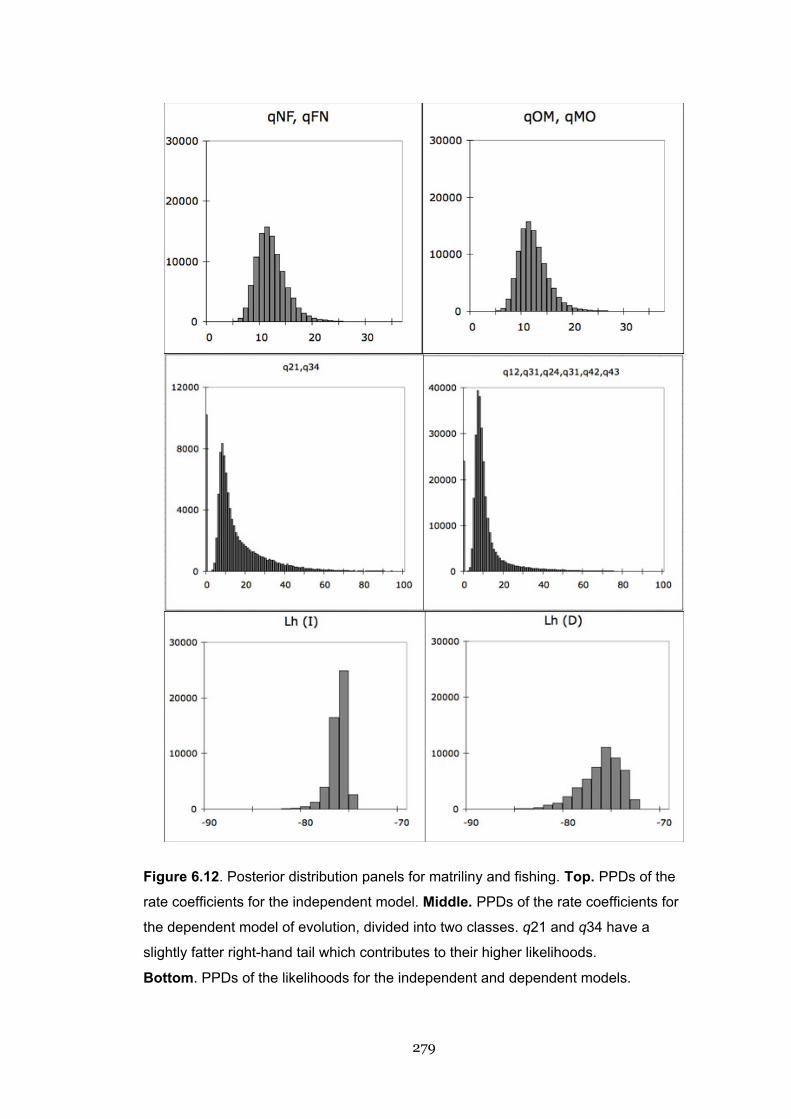
279
Figure 6.12. Posterior distribution panels for matriliny and fishing. Top. PPDs of the
rate coefficients for the independent model. Middle. PPDs of the rate coefficients for
the dependent model of evolution, divided into two classes. q21 and q34 have a
slightly fatter right-hand tail which contributes to their higher likelihoods.
Bottom. PPDs of the likelihoods for the independent and dependent models.

280
In Figure 6.12 the bottom two panels showing the distribution of the
likelihoods for the dependent and independent models demonstrate why the evidence
for correlated evolution is not strong. The two distributions overlap around the same
mean, but the likelihoods for the independent model are tightly clustered compared to
the dependent model. Thus, under the dependent model of evolution there may be
some combinations of tree-topologies and rate parameters that do improve the
likelihood, and, in a single test, would provide evidence of correlated evolution.
However, in this Bayesian context, where we are attempting to control for uncertainty
in our estimates, the probabilistic model demonstrates that we cannot reject the
hypothesis that the two traits are evolving independently.
The top two panels show that under the independent model, both matriliny and
fishing are changing at rates higher than zero, which practically identical distributions.
Based on this, we can infer that both traits are evolutionarily labile, that is, they have
changed back and forth across the phylogeny a number of times. The transition rates
for matriliny have a "longer tail", that is, there are some higher transition rates than
for fishing, but this is not obvious at the scale of the PPD plots.
The RJ MCMC procedure indicates that the second most likely model (below;
Table 6.7) is one that assigns different (higher) rates to the parameters q21 and q34
compared to all others. We can see in the distribution plots of these parameters
(middle left panel) that there are more instances of higher rates, i.e., the right tail is
fatter. This finding is notable because, although we did not find evidence for correlated
evolution, the rates q21 and q34 are the parts of the evolutionary pathway that would
drive an association between matriliny and fishing, as described in Table 6.8.

281
Table 6.9. Matriliny and fishing data showing the most frequent models found by RJ
MCMC model-search, accounting for 24% of all samples. The most-frequent model,
accounting for 10% of all models, has only one parameter, making it equivalent to the
independent model. A total of 1703 unique models were visited, indicating a wide
variety of ways to describe the data. The flow diagram is presented according to the
most-frequent model.
Model string Frequency Cumulative frequency No. of parameters
00000000 4822 0.10 1
00100100 1778 0.13 2
001Z0100 1644 0.16 2
00011Z00 1430 0.19 2
00Z11Z00 1298 0.22 2
001ZZ100 1191 0.24 2
Are there stable states of matriliny and fishing? Together, the second,
third, and sixth most-frequent models account for 4613/50,000, almost as many as the
top (independent) model. These model strings all describe dependent models where
there is a change away from what our hypothesis would predict is an “unstable state”,
that is, the loss of matriliny when fishing dependence is low, and the gain of matriliny
when fishing dependence is high. Here, I test if those models in the sample where q21
and q34 are higher than other rates (the “matri-fish” models) have higher mean
marginal likelihoods than an equal-sized sample of all “other” models. Using the
procedure described above in 6.3.3.4, the likelihood of “matri-fish” models was –74.77,
and the likelihood of “other” models was –77.04, giving a BF = 4.54. Thus, although
there is no evidence for correlated evolution, the data support a hypothesis that non-
matrilineality and low fishing dependence, and matriliny and high fishing dependence,
are stable or attractor states compared to other combinations.
6.4.3.5 Results of an earlier analysis
For comparison, I present here the results of a previous analysis (2002) using the
maximum likelihood version of Discrete (Pagel 1994). This was used to fit the
independent and dependent model of trait evolution on a phylogeny of 34 AN

282
languages derived via parsimony methods (Jordan 1999). The obtained likelihood ratio
(LR) for the model was then compared to a null distribution of likelihood ratios in
order to test for evidence of correlated evolution. A chi-square analysis, the
“traditional” method of testing for a cross-cultural association, was non-significant
(χ2 = 3.33, df = 1, n.s.). However, using the comparative method of Discrete, a
statistically significant association between matriliny and dependence on fishing was
found (LR = 2.06, p < 0.02), indicating that the two characters were evolving together
on the phylogeny. Fixing each rate parameter to zero in a stepwise fashion, and fixing
q21 equal to q34 in order to test for the directionality of this association, revealed no
significant trends. This indicates that the model was assessing ancestral states as
equally probable, and thus for these societies, it may be that matriliny evolved rapidly
and could switch back and forth in the presence or absence of fishing.
6.4.4 Discussion
Using a Bayesian comparative method on ethnographic data from 67 Austronesian
societies, I tested the hypothesis that matriliny co-evolved with a high dependence on
male fishing. Compared to the results of an earlier analysis, and a chi-square test, the
model of correlated evolution was not supported by the data. However, estimates of
the transition-rates to the “stable” states of (i) matriliny and fishing, and (ii) the lack
thereof, revealed that paths leading to the stable states had significantly higher
likelihoods than transitions between all other states.
There are two explanations why positive evidence for co-evolution was not
found. Firstly, there may be an association, but the data and/or the test are insufficient
to reveal it. Secondly, we may require an alternative explanation for the evolution of
matriliny in these cultures.
Using a Bayesian, likelihood-based comparative method meant that the
analysis made use of all the information in the cultural data and the phylogenetic

283
sample (Lewis 2001). The RJ MCMC procedure revealed that dependent co-
evolutionary models were visited frequently, showing that co-evolution is a possible
interpretation of these data. However, no one set of dependent models exceeded the
visits to the independent model, and because of that uncertainty, we cannot accept a
hypothesis of co-evolution. The nature of cross-cultural analyses using sources such as
the Ethnographic Atlas is such that we may be quick to blame our data: it may be
incomplete or inaccurate, we may be comparing apples and oranges, or the pre-
existing coding schemes may be insufficient for the hypothesis. It is unlikely that either
the kinship or the fishing data is biased, as all sources examined were neutral on the
hypothesis.
Using historical linguistics to inform anthropology, Blust (1990), Hage (1998)
have inferred the former presence of matriliny in Austronesian society by cataloguing
or reconstructing kinship terms that are associated with matrilineal organisation, such
as unique terms for the mother’s brother, or matrilateral cross-cousins. Marck (in
preparation) used these kin terms as positive indicators of former matriliny in order to
infer the evolution of Oceanic kinship. In an attempt to use all available information,
in the present test I coded societies that were ambilineal or ambilocal as matrilineal,
making a similar inference that a matrilineal option existed for that society.
What may be lacking is an adequate measure of “male absence”. High
dependence on male fishing may be a sufficient but not necessary cause of matrilineal
social organisation, and may explain why the initial test in the 34-society sample
produced a positive correlation, and why evolutionary transitions towards some states
are more likely. The measure of fishing dependence could be refined with information
on the average fishing range, duration of absence, and risks involved in the method of
fishing, some of which may be extracted from the literature of Pacific fishing (e.g.
Kirch and Dye 1979; Bryan 1984). Male mortality while fishing at sea is recorded
historically as a significant cause of death in Micronesia (Lessa and Myers 1965). As
well, the analyses in Chapter Four indicated that dependence on fishing was associated
284
with geographic nearest neighbours, suggesting that while matriliny may be vertically
transmitted, ecology and/or diffusion may act to “break up” the association with
fishing. Similarly, estimates of male absence may need to incorporate historical and
ethnographic information on the types of trade, voyaging and warfare practised by
each society. Adequate data on warfare exist for those societies in the SCCS, but this
number includes only 11 Austronesian societies (Murdock and White 1969). Pilot
investigations on the feasibility of coding warfare data revealed this to be a
comprehensive task beyond the scope of the present investigation, as scholars of
warfare have attested (Otterbein and Otterbein 1968; Vayda 1978). The task of creating
a comprehensive code for “male absence” is daunting, but may reveal much about
Austronesian social organisation.
Darwinian theory leads us to believe that the “male absence” hypothesis may be
a factor in explaining Austronesian matriliny and matrilocality, even though the
present analysis only offered it as an intriguing possibility. Male absence may be highly
correlated with increased paternity uncertainty, and, as Hartung (1981) and Holden et
al. (2003) have shown, only small levels of paternity uncertainty are required for
female-biased investment (of whatever sort) to be adaptive, for both males and
females. From this, Holden and Mace (2003) argued that matriliny and/or
matrilocality might be a “default” arrangement in the absence of heritable resources
because of a greater relatedness to the matriline, and because matrilineal kin appear to
do more to promote child survival (Mace and Sear 2004). Interestingly, Mace and Sear
point out that it is patrilineal kin who may enhance female fertility. In the
Austronesian context, societies that retain matricentric organisation may be those
more concerned with child survival, while those with patricentric organisation may
have a strategy to increase fertility. These may be the two “stable states” we are seeing
in the flow diagram. This hypothesis offers a fruitful direction for further analysis,
combining information on ecology, environment, and demography.

285
6.4.4.1 Alternative explanations for matriliny
The present study tested only one hypothesis for the evolution of Austronesian
matriliny and matrilocality. Several others in the anthropological literature may be
relevant to the Austronesian situation.
First, Murdock (1949) suggested that matrilocal societies change to become
either patrilocal or avunculocal in the presence of internal warfare, as these patterns
keep unilineal alliances of related males together. However, if there is very high male
mortality (which may be the case in voyaging, trading, or fishing societies as well as
those with high internal warfare), avunculocality, which localises matrilineally-related
men, may be more practical to scattered patrilocality. Second, and related to the
fishing hypothesis, it may be that the sex doing the greatest amount of subsistence-
related work is the one whose kin are localised together (Driver 1956). This predicts
that when males do most of the subsistence work, patrilocal and avunculocal rules will
emerge. When women do more, matrilocal patterns will emerge, and when both sexes
contribute equally, then bi-, neo-, and ambilocal rules will apply. In the Pacific, the
gathering of littoral and reef resources is chiefly women’s work (Kirch and Dye 1979;
Firth 1984; Chapman 1987); this kind of “dependence on fishing” may be a factor in
matriliny, contra the original hypothesis. However, Ember and Ember found no
significant correlations between subsistence contribution and residence rules on a
worldwide data set of 455 societies (1971, 1972), and an opposite association in
Oceania. A number of studies have tested this proposition (Levinson and Malone
1980): it may hold regionally, such as in North America (Driver 1956) or be moderated
by other considerations such as warfare, but the hypothesis remains to be tested
phylogenetically.
Third, recent migration may have some relationship with matricentric social
organisation. Divale (1974) argued that migration (within the last 500 years of the
ethnographic present) into new, but inhabited, areas was likely to be ultimately
responsible for matrilocality. Matrilocality, on this hypothesis, assisted in keeping
286
warfare at bay by dispersing related males in a new territory. There is the intriguing
possibility that Proto Oceanic matrilocality (Hage 1999; Hage and Marck 2003;
Chapter Five) may result from the “incursion” of Lapita-era populations into the
inhabited areas of Island Melanesia.
Lastly, Peregrine (1994) has proposed that incorporation into the world system
produces changes in social organisation through competition and the division of
labour. He argues that societies are “transformed through the introduction of new
trade relations, for the introduction of trade may put pressure on populations to
transform descent and residence toward matrilineal forms” (1994:100). This is a
modern extension of the earlier work by the Embers on warfare: Peregrine argues that
the world system places the same kinds of pressures on a population as does external
warfare. For example, employment in cash industries requires a group of co-ordinated
labour with a single loyalty. Also, female kin can be concentrated in one place in the
face of extended male absences seeking or undertaking work in cities. Using 87
societies from the SCCS, Peregrine examined the introduction of trade into the
subsistence economy of each culture. Using spatial autocorrelation corrections and
linguistic relationships to attempt to control for Galton’s Problem, he found a
significant relationship between (i) trade and matri-focused descent, and (ii) trade and
matrilocality. Peregrine argues that matrilineal groups are “pre-adapted” for world-
system trade, and are also less able to resist trade than other groups. He notes that
long-term extensive incorporation into the world system is likely to break down
unilineal descent systems to bilateral groups or nuclear families, echoing Murdock
(1949), Fox (1967), and others. Careful examination of the ethnographic literature
would be required to operationalise trade and the extent of trading in Austronesian
societies, and crucially, choose appropriate time periods for comparison. Nonetheless,
the hypothesis is relevant, as it can directly speak to whether the processes of change
in kinship organisation are uniformitarian, that is, whether current social change
resembles past processes.

287
6.4.4.2 Does isolation break down matriliny?
Matriliny in Austronesian societies may of course have more than one motivating
factor. If we assume the Proto Austronesian ancestral state to have at least one aspect
of matrilineal organisation (matrilocal residence, Table 5.5), then a complete
explanation will pinpoint factors that have led to the loss of matriliny. Schneider and
Gough (1961) reckoned matriliny to be an unstable type of social organisation, one that
was easily broken down into other forms. In an investigation of kin terminologies in
Oceania, Marck (2006) has suggested that matriliny has undergone a patchwork
pattern of loss. Hage and Marck (2002) have suggested that the cessation of regular
inter-island voyaging (for trading or raiding) may be a factor in those Micronesian
societies that have adopted different forms of residence and descent. Double descent in
the eastern Carolines, where matriliny served only to regulate marriage rules, may
have been such a case: the “relative isolation of the atolls … appears to have promoted
conditions which served to weaken matrilineality” (Damas 1979:192). Isolation, on
their model, means that patriliny or cognatic descent can develop, as the men are no
longer absent. Intriguingly, it appears that the so-called “AD 1300 event”, where
climate cooling led to sea-level falls, a reduction of marine resource availability, and a
shift to inland production rather than coastal exploitation for many Oceanic societies
(Nunn 2003) may have coincided with increased levels of warfare or conflict in (for
example) Tikopia (Kirch 1984) and Tonga (Burley 1998), and after this time, there may
have been a reduction in long-distance voyaging (Rolett 2002). Further work to
identify if and when male absence through voyaging declined, leaving men “at home”,
as well as estimates of the degree of physical and/or social isolation of each society,
may reveal if this explanation can be extended to the Austronesian family as a whole.
288
6.5 Conclusion
Using cutting-edge Bayesian comparative methods, I tested two simple but influential
anthropological models of kinship. One, the “main sequence” theory, was confirmed.
The other, the matriliny and fishing association, was not supported by the data.
Obtaining a positive and a null result on the same data set is encouraging, because it
gives us confidence that our method is not overly generous nor overly stringent.
Because the same tree sample and methodology was used for both sets of tests,
it is possible to remark on the rate of cultural change. Although we did not estimate the
rates of cultural evolution for all traits, we can compare the transition rates of the
matriliny-fishing analysis with that of the main sequence tests. The matriliny-fishing
rates are lower overall that the residence-descent rates, indicating that not only may
individual traits change at different rates, but co-evolutionary rates will vary as well. It
is thus vital that the evolutionary dynamics of each cultural trait are examined
separately, as was seen in Chapter Four.
Pagel and Meade’s (2006) reverse-jump MCMC procedure is extremely useful.
As an heuristic device, the method works by allowing the data to reveal what models
are supported, independent of the hypothesis under consideration. In contrast,
previous implementations of the Discrete algorithm required the investigator to select
which transition were to be made equivalent or set to zero. Not only is this laborious,
but there are ~21,000 different models possible, not all of which are able to be tested.
Cultural traits may evolve quickly or unpredictably, and the RJ procedure lets the data
talk to us directly, indicating the most fruitful avenues for model testing.
The Bayesian framework removes the dependence on any single phylogenetic
hypothesis, and the comparative test becomes "tree-free". Integrating transition-rates
over a tree sample, examining their probability distributions, and seeing, for example,
how often they are in the “zero bin” allows insight into the variability in our
evolutionary scenarios. In this way we make explicit the uncertainty about culture
change that so worries many skeptics of the phylogenetic approach.

289
Both investigations highlighted how crucial a phylogenetic comparative method
is when testing cross-cultural hypotheses, because the conventional chi-square test of
association returned results counter to the phylogenetic analyses. In the main
sequence test, the comparative method provided evidence for co-evolution in both the
coding systems, but the chi-square only showed a significant association for patriliny.
In the matriliny and fishing tests, the chi-square returned a significant association, but
the comparative method found no significant co-evolution. Researchers relying on
non-phylogenetic statistics must control for Galton's Problem, not simply because
their conventional tests may find an association when the data do not support one, but
because they may also fail to detect a real association in the data. Even if we are
skeptical of a phylogenetic comparative approach (e.g. Boyd et al. 1997; Borgerhoff
Mulder 2001; Nunn et al. 2006), the non-phylogenetic alternatives are extremely
unsatisfactory. In contrast, a Bayesian approach allows us to account for uncertainty
about population history, estimate the uncertainty in adaptive hypotheses, and develop
illuminating models of evolutionary relationships.
290
CHAPTER SEVEN
EVOLUTIONARY ANALYSES OF LEXICAL CHANGE AND POPULATION SIZE
7.1 Summary
Aspects of language vary in their rates of evolution and subsequently different
languages may accumulate different amounts of lexical (word) change once they split
from a common ancestor. These differences may be produced by a number of factors;
here I tested for an association between lexical change and a demographic variable,
population size, in the Austronesian languages. Conventional correlation analyses
revealed a significant inverse relationship, suggesting that as population size
increased, lexical change decreased. However, phylogenetic comparative methods
found no evidence for correlated evolution, demonstrating the need to control for
shared descent in cross-cultural analyses. Scaling parameters in the phylogenetic
method showed how the two traits were evolving under different evolutionary models.
Population size could be characterised by a punctuational and/or random drift model,
whereas lexical change had a directional aspect and showed evidence for adaptive
radiation. Plotting the two traits according to the power law distribution supported
these conclusions. Alternative explanations for lexical change in Austronesian
languages are considered.
291
7.2 Introduction
7.2.1 Language change
Factors affecting language change tend to be well-described for individual languages,
yet general cross-cultural principles, especially those concerning the rate of change, are
not well known. A constant rate of linguistic change (in basic vocabulary) was assumed
in early lexicostatistical work (Swadesh 1951), and Nicholls (1992) assumed linear
rates of change in estimating patterns of worldwide linguistic diversity. Nettle (1998)
questioned the rate-constancy assumption, arguing that linguistic change declined
over time following radiation of ethnolinguistic groups into new areas. However, there
have been no quantitative evolutionary tests of the factors causing differential rates of
change. Linguistic change can be seen as an expression of the larger dynamics of
cultural change, and so we may approach questions of language change with the theory
and methods of cultural evolution.
The sources of variation in language change can come from imperfect learning
(i.e. mistakes in the transmission of variants from parent to offspring), from deliberate
change (either individual or group consensus) and from one-off performance variants
(Lindblom 1995). Factors that may affect language change include the method of
language transmission to children, the degree and type of contact with other
communities and/or their languages (including the degree of bilingualism), and other
social factors such as name or word taboos (Crowley 1997). Demographic factors and
population dynamics may have an effect at the intra-group level by affecting how
quickly language changes are passed on to the next generation, and at the inter-group
level by contributing to the levels of diversity in daughter languages. Nettle (1999b)
argues from Nichols (1992) data that language diversity—as expressed in languages per
stock—is greater in the New World and Australia/Pacific due to smaller overall
population sizes. Here we are mainly concerned with population size effects at the

292
between-language level: how might population size affect the rate of evolutionary
change?
7.2.2 Founder effects
In biology, the founder effect (Mayr 1963) is a sampling effect that refers to the
establishment of a new population by a small group of founders who carry some
reduced amount of the genetic variation of the original population. Stochastic effects
(genetic drift) on small samples can mean the variation in the new population is very
different to the original. Founder effects can be caused by migration, by population
subdivision without migration, or by population bottlenecks (fluctuation in size due to
some retardation on population growth). As well, the effects of random variation on
small populations are greater due to the lack of demographic buffer. Founder effects
and genetic, cultural, and linguistic drift are all features of Austronesian population
history. Polynesian populations represent the end-point of consecutive voyages by
small populations from Island Southeast Asia, and as such, some genetic markers such
as the substitution motifs accompanying the 9bp deletion are at high fixation rates
compared to source populations (Melton et al. 1995). Blust (1981a) notes that
consonants decrease in number in languages as one travels eastwards across the
Pacific, leaving only eight in Hawaiian, and similarly, many items of material culture
such as metalworking, loom weaving, and pottery decline in the same direction (Blust
1995). Population crashes on small and/or ecologically vulnerable islands also
exacerbate the stochastic nature of drift. For example, Typhoon Lengkiekie devastated
the atoll Pingelap (Micronesia) in 1775, reducing the population drastically. A ~30%
prevalence of autosomally-recessive achromatopsia (colour-blindness) in the present-
day population has been linked to this event (Sacks 1997; Sundin et al. 2000).

293
7.2.3 Punctuated equilibrium
Dixon (1997) borrowed the concept of punctuated equilibrium (Eldredge and Gould
1972) from evolutionary biology and applied this to language change. On this model,
the majority of change is slow and gradual, with most linguistic innovations
languishing un-transmitted in a single generation. Demographic or ecological factors
cause disruption to the social system in some fashion, often through migration or
technological innovation, and this causes a cascade of rapid and significant change in
language. Thus, repeated punctuation events give rise to the hierarchical branching
tree model of language evolution, as subdivided populations become linguistically
isolated from one another. The punctuation model may be of especial significance in
the Austronesian family, where not only is the family expansion as a whole thought to
be driven by the engine of agricultural technology (Diamond and Bellwood 2003), but
where a series of repeated migrations to island environments characterised the
Oceanic phase of expansion. These migration events are essentially demographic
changes, and as such, an examination of the effect of population size on language
change is warranted.
7.2.4 Demography and the rate of change in biosocial variables
Demographic variables such as fertility rates, sex ratios, and population size are often
included in cross-cultural comparisons either as determinants of some biosocial
variable or as the dependent variable itself. For example, Mace and Jordan (2005)
found that a female-biased sex ratio at birth in African countries might be associated
with the greater physiological costs of producing male babies, but was not associated
with the presence of bridewealth. However, no studies to date have examined the effect
of population size on the rate of evolutionary change in some human biosocial variable.
This is remarkable considering that the effects of population size on diversity and rates
of evolution have been discussed in the theoretical and experimental population

294
genetics literature since Wright (1931), and mathematical treatments of cultural
evolution have also included population size in their equations (Cavalli-Sforza and
Feldman 1981; Boyd and Richerson 1985).
The paucity of research may be because it is difficult to obtain data on
population size for cross-cultural analysis. While census information at a country level
is usually freely available e.g. The CIA World Factbook,
(https://www.cia.gov/cia/publications/factbook), and the Demographic and Health
Survey project (http://www.measuredhs.com) provides village or town level
population numbers, the investigator is often left with large gaps in the analysis. Many
studies have thus resorted to using country-level statistics, which by their aggregate
nature are unsatisfactory when dealing with ethnolinguistic groups that may be spread
over two or more countries, or who may be only one of many groups in a country.
Other information sources such as the Ethnographic Atlas or the Standard Cross-
Cultural Sample contain limited population information, often only expressed in 3–5
classes, and in the case of the former, much of this is missing for Pacific cultures.
One source that contains population figures for individual languages is the
Ethnologue (Gordon 2005). Here, numbers refer not to the demographic population
but rather the number of language speakers at a recent point in time. As such, this
figure can be thought of as equivalent to the effective population size (Ne) or “breeding
population” (Wright 1931), as it represents the number of individuals able to transmit
the language to the next generation. This is thus a more suitable variable than standard
population numbers. It will of course be an approximate estimate, but the figures are
available for all 67 languages in the Austronesian sample, allowing hypotheses about
the rate of change to be tested.
7.2.5 Modelling the rate of word evolution
Lexical items (words) constitute one aspect of the linguistic system that can be
examined as an evolving cultural trait. Other features might be aspects of typology,

295
such as word order, or phonology (sound change). The method of glottochronology
(Swadesh 1955) was an attempt to understand the rate of lexical replacement in
languages as similar to a radioactive decay function. Glottochronology was an
approach to estimating the time-depth of a lexicostatistical tree and used a formula
specifying the relationship between shared cognate percentages, a universal retention
rate, and time depth in millennia. Numerous flaws with lexicostatistical and
glottochronological methods mean these approaches are largely discredited (Bergsland
and Vogt 1962; Blust 1999; Campbell 2004). The most trenchant criticism, that these
methods did not distinguish shared innovations from shared retentions, is addressed
by the use of phylogenetic methods that use only synapomorphies (shared evolutionary
innovations) to build trees. Newer methods to estimate the rate of word evolution have
employed phylogenetic statistical models to assess the rate of evolutionary change in
lexical items and test hypotheses about language dating in the Indo-European
language family (Gray and Atkinson 2003). These Bayesian methods look to be the
most productive avenue for research aimed at dating ancestral languages/cultures or
assessing the rate of change in cultural traits.
Other workers have used computer simulations to investigate the dynamics of
lexical change. Nettle (1999a) simulated language change by modelling social and
functional (adaptive) selection on the uptake of new words in a population. He found
that influential individuals who adopt a new word were a major factor in the dynamics
of language change, and related these findings to the “threshold problem”. Unlike the
genetic situation where a mutation has a high probability of being passed on to the
next generation, linguistic mutations are less likely to be passed on due to (i) a higher
number of cultural parents, and (ii) conformity bias, the tendency to copy the most
common variant (Boyd and Richerson 1985). Further work by Nettle (1999b)
simulated population size effects on the rate of language change, because as population
size increases, the threshold problem is magnified: “As community size increases,
then, the probability of some individual adopting a rare variant q becomes smaller, and

296
the number of such adoptions which are required for q to become the community
norm increases.” (1999b:123). Nettle’s simulation found that the rate of change
declined with increasing community size. What could be the proximate mechanisms of
this relationship? The rate of change in languages of large population size may be
affected by institutions that act to maintain linguistic homogeneity, such as schooling
norms or a body of written literature. In smaller populations, it may be that language
norms are more likely to be vertically transmitted only, and thus more prone to
copying errors.
The attempts to model the evolutionary dynamics of lexical change have shown
that a phylogenetic perspective is required, and that population size may be a factor in
the rate of change. Other approaches consider a null model of neutral change.
7.2.6 Models of neutral or random change
Demographic estimates are important components in modelling the patterns of
diversity and/or coalescent (times to most recent common ancestor) of gene markers.
For example, genetic studies have calculated that the human species is relatively young
in terms of genetic diversity, undergoing a bottleneck c.100,000 years ago in Africa,
where the population was limited to only about 1000–10,000 individuals (Harpending
et al. 1997; Underhill et al. 2001). In population genetics, the neutral model (Kimura
1968) describes how the vast majority of evolutionary change is due to the random
fixation of selectively neutral alleles. As a consequent, neutral theory states that in the
absence of other evolutionary forces (e.g. selection, migration, mutation) the
probability of fixation of a new allele in a population is inversely related to population
size, as proposed by Wright (1931). In the genetic situation, this relationship is
moderated by a corresponding increase in the overall mutation rate producing similar
variants. In the linguistic situation there may not be the same eliminating selection on
these variants, and so the balance created by an increase mutation rate may not hold
for language change (Nettle 1999b), thus allowing population size to affect the rate of

297
change. By identifying departures from a constant-variance or neutral model of
evolution, we can infer the presence of additional evolutionary forces.
Power laws have been invoked to explain the distribution properties of many
real-world systems such as language. For example, word frequencies in usage are
inversely proportional to their rank (Zipf 1949). Power laws describe a decay curve that
plots as a straight line on a log-log scale; as they are supposedly a feature of self-
organising systems (Bak 1996) they can thus seen as a null or random change model,
akin to neutral drift in population genetics (Hahn and Bentley 2003). Recently,
Bentley et al. (2004) have demonstrated that aspects of culture such as popularity in
baby names, dog breeds, and patent citations conform to this law through a random
copying process. Departures from the power law may indicate processes other than
random change at work in a system, for example, in their study of dog breed popularity
through time, Hertzog, Bentley, and Hahn (2004) found that Dalmatians did not
conform to the power law, probably due to films that popularised the breed. With
respect to language, Wichmann (2005) ranked world language families by the number
of languages they contained and found that they conformed to the power law
distribution, but the number of speakers in each language did not demonstrate this
relationship. Similarly, we can rank languages in a single family according to their
amount of lexical change or their population size to see if they conform to the power
law distribution.
7.2.7 Aims of the study
Here I examine the evolutionary processes affecting (i) language population size and
(ii) the amount of lexical change using empirical data from the Austronesian language
family. Some authors (Borgerhoff Mulder 2001) have questioned whether phylogenetic
controls are necessary in cross-cultural tests; here, a number of conventional and
phylogenetic comparative methods are employed, as it is not possible to determine the
need for historical control a priori. This serves as a demonstration case for the

298
phylogenetic approach. The purpose is to characterise the tempo and mode of
evolution of population size and lexical change by seeing if they evolve according to a
constant-variance model of change, and to test for any co-evolutionary relationship
between the two traits. If founder effects cause greater differentiation in daughter
populations through the “fixation” of random effects, we should expect that small
populations are more different to the source population than are large populations.
Thus, we might predict an inverse relationship between population size and the
amount of lexical change.
7.3 Data
7.3.1 Demographic data
Data on population size were obtained from the online version of the Ethnologue
(Gordon 2005). These data are approximate numbers, indicating the number of
current speakers rather than being a demographic indicator of population. There will
be inconsistencies between the dates when the language population data were
recorded and the dates when each language itself was recorded. In some cases, the
population sizes may be underestimates of the ethno-linguistic population due to
language or population decline. In other cases they may be large overestimates; some
languages such as Malay and Javanese have speakers in the millions in the highly
populous islands of Indonesia, and many of these speakers may be bi- or tri-lingual in
other languages. However, we should not expect the population size estimates to be
systematically biased with respect to the hypotheses. Population estimates were log-
transformed and were found to approximate a normal distribution.
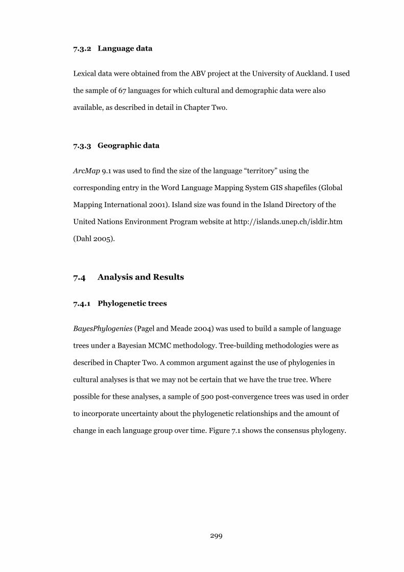
299
7.3.2 Language data
Lexical data were obtained from the ABV project at the University of Auckland. I used
the sample of 67 languages for which cultural and demographic data were also
available, as described in detail in Chapter Two.
7.3.3 Geographic data
ArcMap 9.1 was used to find the size of the language “territory” using the
corresponding entry in the Word Language Mapping System GIS shapefiles (Global
Mapping International 2001). Island size was found in the Island Directory of the
United Nations Environment Program website at http://islands.unep.ch/isldir.htm
(Dahl 2005).
7.4 Analysis and Results
7.4.1 Phylogenetic trees
BayesPhylogenies (Pagel and Meade 2004) was used to build a sample of language
trees under a Bayesian MCMC methodology. Tree-building methodologies were as
described in Chapter Two. A common argument against the use of phylogenies in
cultural analyses is that we may not be certain that we have the true tree. Where
possible for these analyses, a sample of 500 post-convergence trees was used in order
to incorporate uncertainty about the phylogenetic relationships and the amount of
change in each language group over time. Figure 7.1 shows the consensus phylogeny.
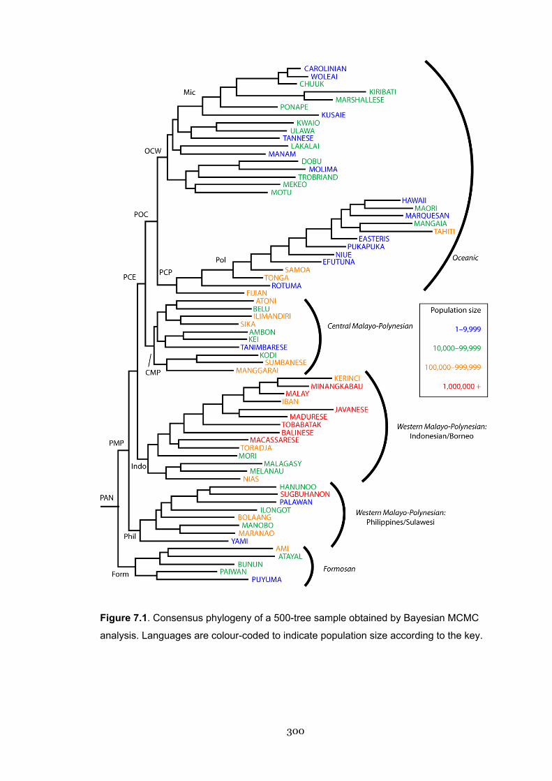
300
Figure 7.1. Consensus phylogeny of a 500-tree sample obtained by Bayesian MCMC
analysis. Languages are colour-coded to indicate population size according to the key.

301
7.4.2 Calculating language change
Tip-to-root distances were calculated for each language as an estimate of the amount
of language change (lexical replacement). These distances were calculated by summing
the total path lengths along the path from the root using a UNIX program written for
this purpose (TipToRoot, A. Meade, personal communication). The figures obtained by
this program were not units of lexical change per se, but were rather the posterior
probabilities of change along the branch. Thus the total path length for each language
was multiplied by the overall number of characters to give an index, Total Lexical
Change (TLC) that was used as the measure of lexical change in the subsequent
analyses. TLC values were calculated for all languages over all 500 trees. From these, I
calculated the mean TLC for each language, shown in Table 7.1. Figure 7.2 shows a
representative distribution of the TLC for two languages, Ambon and Yami.
Figure 7.2. The root-to-tip distance or total lexical change (TLC), for two languages,
Ambon and Yami, across a sample of 250 trees. All languages followed this slightly
left-skewed distribution, showing a large number of TLC values about the mean and a
few, more extreme values at the right tail of the distribution.

302
Table 7.1. Language groups used in the analyses. The table shows the number of
speakers, the mean total lexical change of each language derived from a sample of
500 trees, mean terminal branch length (TBL) demonstrating language-specific
amounts of change, and the ranking of each language in terms of amount of change
(1 = highest).
Language Number ofspeakers
(POP)
Mean totallexical change
(TLC)
Mean terminalbranch length
(TBL)
POPRank
TLCRank
Ambond 15965 594.92 68 43 54
Ami 130000 697.98 129.12 22 39
Atayal 63000 996.04 129.56 27 9
Atoni 586000 661.75 69.80 11 44
Balinese 3800000 717.23 110.92 6 35
Belu 50000 597.01 69.80 32 53
Bolaang 900000 653.96 122.04 9 46
Bununa 34000 711.93 129.68 36 37
Caroliniand 3000 827.97 77.04 60 23
Chuukd 38341 844.96 77.56 35 19
Dobuc 10000 1038.93 85.36 50 7
Easter Is.b,d 2450 869.75 96.88 61 16
East Futunab,d 3600 843.48 99.88 56 20
Fijian 330441 742.39 103.88 16 31
Hanunoo 11000 559.57 122.16 48 59
Hawaiib 1000 960.13 92.88 66 12
Iban 400000 536.13 110 15 65
Ilimandiri 150000 670.40 70.48 21 42
Ilongot 50786 810.85 121.96 31 25
Javanesea 75200000 806.22 111.04 1 26
Keid 86000 587.99 68 26 57
Kerinci 300000 633.30 108 17 47
Kiribatid 58320 1138.21 79.60 29 3
Kodi 40000 720.03 72.52 34 34
Kusaied 6900 1158.12 80.64 55 2
Kwaioc 16700 918.08 85.96 42 14
Lakalaic 13000 985.17 89.88 46 10
Macassaresea 1600000 654.57 110.56 8 45
Maduresea 13000000 594.27 111.04 3 55
Malagasy 88000 736.79 117.60 25 33
Malaya 10000000 531.18 109 4 66
Manamc 7000 840.30 87.44 54 21
Mangaiab,d 16800 896.40 94.88 41 15

303
Table 7.1 (Continued). Language groups used in the analyses.
Language Number ofspeakers
Mean totallexical change
Mean terminalbranch length
POPRank
TLCRank
Manggarai 500000 589.98 73.52 13 56
Manobo 12500 542.30 124.28 47 63
Maorib 60000 984.00 92.88 28 11
Maranao 776169 529.33 124.28 10 67
Marquesanb,d 3400 942.68 93.88 57 13
Marshallesed 43900 803.19 79.28 33 27
Mekeoc 25120 1002.26 87.36 40 8
Melanau 19000 540.00 117.64 38 64
Minangkabaua 6500000 601.56 108 5 51
Molimac 3186 1078.60 85.36 58 5
Mori 15000 632.73 115.44 44 48
Motuc 14000 790.49 87.36 45 28
Nias 480000 620.60 118.40 14 50
Niueb,d 2240 781.86 98.88 62 29
Paiwan 53000 543.46 130.72 30 62
Palawan 2041 597.15 123.20 63 52
Ponaped 27700 862.17 80.56 37 17
Pukapukab,d 840 846.31 97.88 67 18
Puyuma 7225 625.65 130.76 53 49
Rotumad 9000 816.70 102.88 51 24
Samoab 199377 744.70 100.88 19 30
Sika 175000 571.34 70.48 20 58
Sugbuhanona 14713220 558.32 122.48 2 60
Sumbanese 234000 683.66 72.52 18 41
Tahitib 117000 1054.16 94.88 23 6
Tanimbarese 8000 713.04 73.32 52 36
Tannesec,d 2000 1158.98 86.16 64 1
Toba Bataka 2000000 668.34 112.92 7 43
Tongab,d 103200 690.91 101.84 24 40
Toradja 500000 548.05 110.52 12 61
Trobriandc,d 22000 1102.31 86.36 39 4
Ulawac,d 10700 740.01 85.96 49 32
Woleaid 1631 830.58 77.40 65 22
Yami 3000 711.36 126.12 59 38
1. Number of speakers obtained from the Ethnologue.2. Total lexical change obtained by multiplying the posterior probability of change by the
number of cognate changes in the data set (17464).a: “Super-language”: population size over one million. b: Polynesian language. c: Territory/island size less than 1000 sq km. d: “Contact” language: a language geographically situatednear Non-Austronesian languages, around the coast of New Guinea.
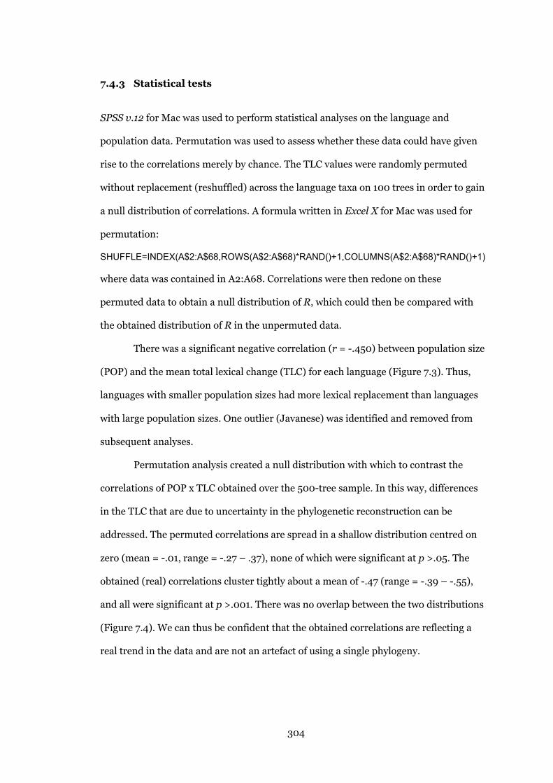
304
7.4.3 Statistical tests
SPSS v.12 for Mac was used to perform statistical analyses on the language and
population data. Permutation was used to assess whether these data could have given
rise to the correlations merely by chance. The TLC values were randomly permuted
without replacement (reshuffled) across the language taxa on 100 trees in order to gain
a null distribution of correlations. A formula written in Excel X for Mac was used for
permutation:
SHUFFLE=INDEX(A$2:A$68,ROWS(A$2:A$68)*RAND()+1,COLUMNS(A$2:A$68)*RAND()+1)
where data was contained in A2:A68. Correlations were then redone on these
permuted data to obtain a null distribution of R, which could then be compared with
the obtained distribution of R in the unpermuted data.
There was a significant negative correlation (r = -.450) between population size
(POP) and the mean total lexical change (TLC) for each language (Figure 7.3). Thus,
languages with smaller population sizes had more lexical replacement than languages
with large population sizes. One outlier (Javanese) was identified and removed from
subsequent analyses.
Permutation analysis created a null distribution with which to contrast the
correlations of POP x TLC obtained over the 500-tree sample. In this way, differences
in the TLC that are due to uncertainty in the phylogenetic reconstruction can be
addressed. The permuted correlations are spread in a shallow distribution centred on
zero (mean = -.01, range = -.27 – .37), none of which were significant at p >.05. The
obtained (real) correlations cluster tightly about a mean of -.47 (range = -.39 – -.55),
and all were significant at p >.001. There was no overlap between the two distributions
(Figure 7.4). We can thus be confident that the obtained correlations are reflecting a
real trend in the data and are not an artefact of using a single phylogeny.
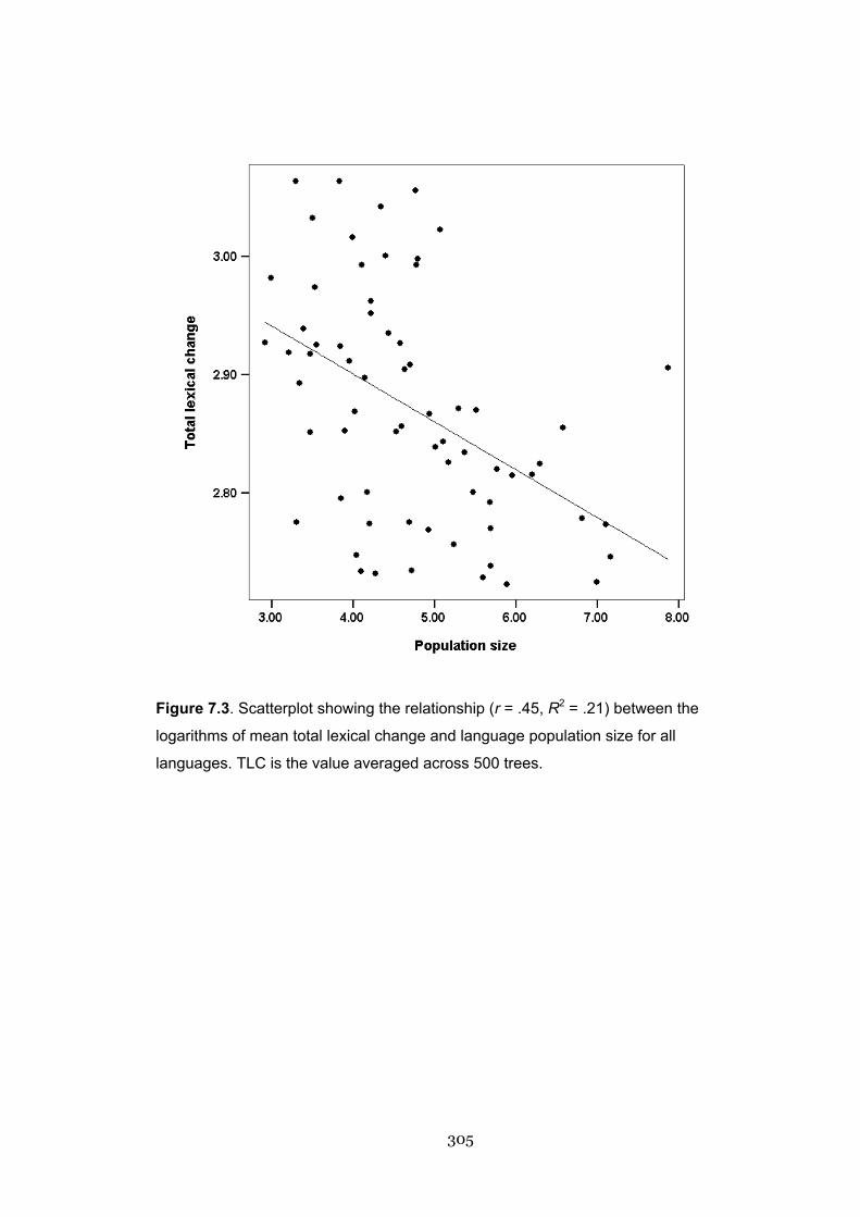
305
Figure 7.3. Scatterplot showing the relationship (r = .45, R2 = .21) between the
logarithms of mean total lexical change and language population size for all
languages. TLC is the value averaged across 500 trees.
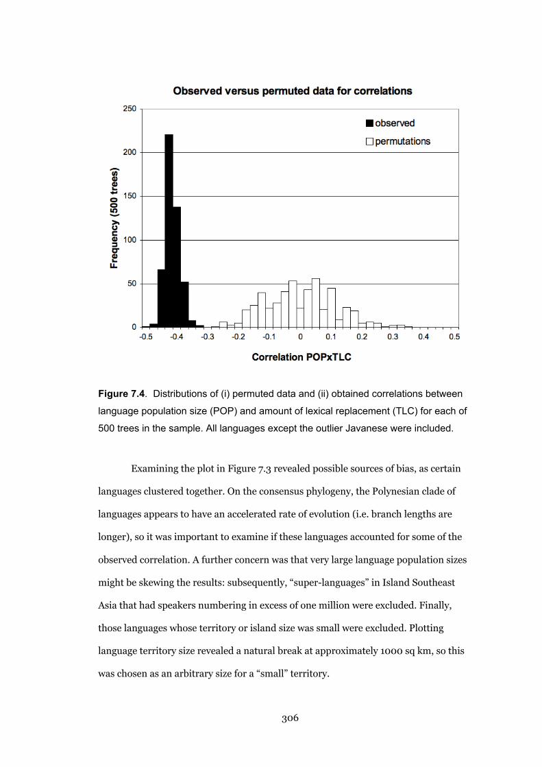
306
Figure 7.4. Distributions of (i) permuted data and (ii) obtained correlations between
language population size (POP) and amount of lexical replacement (TLC) for each of
500 trees in the sample. All languages except the outlier Javanese were included.
Examining the plot in Figure 7.3 revealed possible sources of bias, as certain
languages clustered together. On the consensus phylogeny, the Polynesian clade of
languages appears to have an accelerated rate of evolution (i.e. branch lengths are
longer), so it was important to examine if these languages accounted for some of the
observed correlation. A further concern was that very large language population sizes
might be skewing the results: subsequently, “super-languages” in Island Southeast
Asia that had speakers numbering in excess of one million were excluded. Finally,
those languages whose territory or island size was small were excluded. Plotting
language territory size revealed a natural break at approximately 1000 sq km, so this
was chosen as an arbitrary size for a “small” territory.
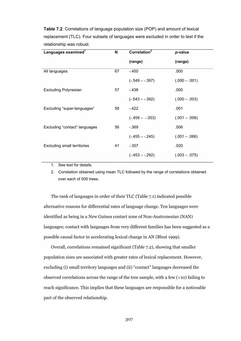
307
Table 7.2. Correlations of language population size (POP) and amount of lexical
replacement (TLC). Four subsets of languages were excluded in order to test if the
relationship was robust.
Languages examined1 N Correlation2
(range)
p-value
(range)
All languages 67 -.450
(-.549 – -.397)
.000
(.000 – .001)
Excluding Polynesian 57 -.438
(-.543 – -.392)
.000
(.000 – .003)
Excluding “super-languages” 58 -.422
(-.459 – -.353)
.001
(.001 – .006)
Excluding “contact” languages 56 -.369
(-.455 – -.245)
.006
(.001 – .066)
Excluding small territories 41 -.357
(-.453 – -.292)
.020
(.003 – .075)
1. See text for details.
2. Correlation obtained using mean TLC followed by the range of correlations obtained
over each of 500 trees.
The rank of languages in order of their TLC (Table 7.1) indicated possible
alternative reasons for differential rates of language change. Ten languages were
identified as being in a New Guinea contact zone of Non-Austronesian (NAN)
languages; contact with languages from very different families has been suggested as a
possible causal factor in accelerating lexical change in AN (Blust 1999).
Overall, correlations remained significant (Table 7.2), showing that smaller
population sizes are associated with greater rates of lexical replacement. However,
excluding (i) small territory languages and (ii) “contact” languages decreased the
observed correlations across the range of the tree sample, with a few (<10) failing to
reach significance. This implies that these languages are responsible for a noticeable
part of the observed relationship.

308
7.4.3.1 Language-specific change
The total path length expressed by the TLC variable contains some phylogenetic
structure, as any two languages may share a certain amount of that total path length.
Thus, the terminal branch length (TBL) was used as a metric to quantify the amount of
language-specific change, i.e. the amount of change since splitting from its final sister
taxa. The branch-length table output in PAUP* was used to find the TBL for each taxa,
for 30 randomly selected trees from the Bayesian sample. The mean value of TBL for
each language is listed in Table 7.2. TBL was correlated with POP and with mean TLC
over a random sample of 30 phylogenies as shown in Table 7.3.
Table 7.3. Terminal branch lengths (TBL) correlated with population size (POP) and
overall path length (TLC).
Correlation (range) p-value (range)
TBL x POP .238 (.226 – .253) .053 (.039 – .066)
TBL x TLC -.278 (-.287 – -.266) .023 (.019 – .030)
The correlation between population size and terminal branch length is
moderate and reaches the .05 level of significance on slightly less than half of the trees.
When it does, the relationship is positive, in the opposite direction of the correlation of
population size with TLC, implying that larger populations have more lexical change.
However, there is a great deal of uncertainty in this association, as it appears to be
contingent on the particular phylogeny. There is an inverse and significant relationship
between total path length and terminal branch length, which suggests that high overall
divergence is associated with less language-specific change and/or that low levels of
overall change have a greater proportion of change in terminal branches. From this, an
adaptive radiation process could be inferred, with greater probabilities of change in
early branches on the tree.
309
7.4.5 Phylogenetically controlled analyses
Conventional statistical tests have shown a correlation between population size and the
overall amount of lexical change. It could be argued that population size is reduced and
created anew as each language group fissions, and as such, it is a variable without a
phylogenetic history. The preceding tests attempted to reduce possible confounds by
excluding languages that appeared to cluster in the correlation, but we cannot be
certain that this is sufficient historical control. Here, a comparative method is used to
investigate any effects of phylogeny on population and language change, both
separately and by testing for co-evolution.
Pagel's Continuous (1997) uses a generalised least squares (GLS) comparative
method that investigates how continuously varying traits evolve on a phylogeny. This
method is appropriate for tests of language rate and population size, as both characters
vary continuously. Characters may accumulate evolutionary change with constant
variance, that is, by Brownian motion, such that the number of changes is proportional
to the time or distance along the branches of the tree. In assessing whether the
assumption of constant variance is true for each character, Continuous estimates a
number of parameters that reveal information about the nature of the evolutionary
process. These parameters set the method aside from other comparative tests such as
Felsenstein’s (1985) independent contrasts (Pagel 1997). Continuous also allows us to
test for co-evolution.
Across all taxa, each trait value can be described by a regression equation. This
equation relates the total path length from root to tip of each language and the value of
the trait (Pagel 1997). The beta coefficient is the "slope", and, if taxa are independent,
can be estimated by a standard regression. Phylogenetic structure means that two taxa
will share at least some of their total path length. If taxa share much of their total path
length, they will have similar values of the trait. Therefore, the beta value must be
adjusted for a specified level of non-independence. To do this, a shared variance-
covariance matrix is derived from the shared path lengths over the whole phylogeny

310
and for all pairs of species. In effect, this provides a null model of the expected
proportion of covariance we expect due to phylogeny.
Continuous v.1 was used with the 67-language data set. The Nexus file of the
consensus phylogeny of 1000 trees was converted to “*.pag” file format and annotated
with two columns of comparative data: (i) the root-to-tip lexical changes and (ii)
population size. Both variables were log-transformed in the program. Except where
noted, all tests involved comparing a null (H0) and alternative model (H1) in a nested
log-likelihood ratio (LR) test. A nested test is one where the alternative model has an
extra parameter compared to the null i.e. the null is a simpler case. This test compares
the goodness of fit of these models to the data. The LR statistic is calculated as
-2 loge (H0/H1) and is distributed as approximately χ2 with degrees of freedom
equivalent to the difference in the numbers of parameters between the two models.
7.4.6 Drift versus directional models of evolution
In this test we compare two models. The random-walk model estimates the standard
constant-variance model of evolution, which is equivalent to drift. The directional
model estimates an extra directional parameter that indicates if there is any trend in
the value of the trait(s) from root to tips. Applied to these data, the directional model
would suggest that lexical change is accumulating faster (or slower), and that
population size is getting bigger or smaller.
The directional model fits the language change trait better than the constant
model (LR = 75.37, p = .000, d.f. = 1). Thus, lexical change is not accumulating at some
metronomic rate through time, but rather, it is affected by other evolutionary
processes that are causing change to speed up or slow down. Population size, however,
fits the simpler drift model and does not show any trend across the tree (LR = .12, p =
.624, d.f. = 1). Large populations are not giving rise to larger ones or vice versa. When
the two traits are allowed to co-vary, we can estimate the best-fit model
simultaneously. Again, the simple drift model applies to the combined traits (LR = .19,
p = .535, d.f. = 1).

311
7.4.7 Mode and tempo of evolution
Three informative scaling parameters can be estimated from the data. The following
descriptions come from the software manual for Continuous, available at
http://www.evolution.rdg.ac.uk/SoftwareMain.html.
Kappa (κ) is a parameter that scales branch lengths and can be used to infer a
punctuational or gradual mode of evolution (Pagel 1997). A value of κ between zero
and one implies a model where short branches have many changes, with κ=0
indicating punctuational evolution and κ=1 indicating a default gradualism, that is,
change proportional to branch length. Values of κ greater than 1 mean that there is
more change on long branches.
Lambda (λ) assesses the contribution of phylogeny to the model and promises
to be a useful diagnostic tool for deciding which comparative method to choose
(Freckleton et al. 2002). It takes a value between zero and one, where λ=0 indicates
that the phylogenetic correction is not necessary for the trait (the phylogeny is
effectively a star), and where λ=1 means that the trait is evolving according to the
default phylogeny. Intermediate values indicate the degree to which phylogenetic
history will affect how the model of evolution is estimated.
Delta (δ) detects differential rates of evolution over the course of time in the
phylogeny by scaling the root-to-tip distances. A value of δ=1 indicates default
gradualism, while δ<1 suggests that change occurred early in the tree—evidence for
adaptive radiation. Values of δ greater than one thus suggest taxa-specific adaptation,
that is, change occurring in the latter, possibly terminal branches of the tree.
The scaling parameters were estimated for both traits separately and then
simultaneously by allowing the two to co-vary. Then, the fit of a model where they were
allowed to take their maximum-likelihood estimate was compared to one where they
were set to the default gradualism value of one.

Table 7.4. Maximum-likelihood estimates of three scaling parameters showing how three traits evolve on a phylogeny: population size, amount of
overall lexical change, and amount of language-specific change. Significant departures (in bold) from the default gradualism model are determined
by likelihood ratio tests. Parameters were estimated under the drift or directional model determined to best fit the data.
Kappa (κ)
Punctual v. gradual
Lambda (λ)
Contribution of phylogeny
Delta (δ)
Early v. late change
ML estimate
(95% C.I.)
LR test ML estimate
(95% C.I.)
LR test ML estimate
(95% C.I.)
LR test
Population size§ .34
(.00-.77)
LR = 4.41
p = .00
.69
(.35-.95)
LR = 3.67
p = .01
1.29
(.59-2.10)
LR = .31
p = .43
Total lexical change§§ .98
(.93-1.04)
LR = .08
p = .69
1.00
(.89->1.00)
LR = 0
p = 1
.24(.00-.57)
LR = 8.37
p = .00
POP x TLC coevolving .98
(.92-1.04)
LR = .30
p = .44
.91
(.68->1.00)
LR = .93
p = .17
.40
(.15-.72)
LR = 4.68
p = .00
Terminal branch length§ .00
(.00-.06)
LR = 8.97
p = .00
1.00
(.98->1.00)
LR = 0
p = 1
.05
(.00-.22)
LR = 7.03
p = .00§ Estimated under the constant-variance (drift) model. §§ Estimated under the directional model.
Abbreviations: lang. = language, Pop. = population, LR = likelihood ratio test statistic, CI = confidence interval. All tests have d.f. = 1.
312
313
The kappa value for population size is less than one and indicates that short
branches contain proportionately more changes than long branches. Thus, a
punctuational model of change in population size is appropriate and makes intuitive
sense. Lambda values for population are also below one, suggesting that phylogeny has
a reduced effect on this trait. There is a trend towards temporally later change, shown
by the delta value greater than one, but the LR test does not distinguish this trend as
significantly different from the gradual assumption.
The opposite pattern is obtained for the overall language change variable. Here,
the gradualism model applies to both kappa and lambda because their ML estimates
are not a significantly better fit than the default value of one, indicating that
phylogenetic control is important. The delta parameter suggests that most change
occurs in the early branches of the phylogeny, and an adaptive radiation model is
appropriate. This pattern also applies to the parameters when the traits are allowed to
co-evolve together.
Language-specific change appears to be evolving under a punctuational model
according to the kappa value of zero; the delta parameter (also zero) indicates that this
change may have taken place early in the phylogeny. The lambda value suggests there
is phylogenetic structure to the data, so, although most of the phylogenetic splitting
may have been compressed to a short punctuational burst, closely related languages
continue to evolve lexical change at the same rate in their terminal branches.
7.4.8 Phylogenetic tests of correlated evolution
We may test the hypothesis that the two traits are evolving together on the tree by
comparing a model where the traits are allowed to take their ML estimates to one
where their co-variances are set to zero. This is a phylogenetically controlled version of
the conventional correlation in §7.4.3, removing the proportion of covariance between
taxa that is due to shared path lengths on the tree. The correlation reduces from r = -
.49 in the conventional test to r = -.09 with phylogenetic control. The LR test finds that

314
this is not significantly different from a co-variance of zero (LR = .26, p = .473). The
lambda estimate of population size by itself indicated that this trait does not seem to
be influenced much by phylogeny and all observations could possibly be treated as
independent. However, the disappearance of the significant correlation with the
comparative test suggests that any concerted change in the two traits was likely caused
by similarity due to descent. Correlations using the language subsets in Table 7.2 were
also not significantly different from zero in all case. Similarly, there was no correlation
between language-specific change (TBL) and population size (LR = .025, p = .825).
7.4.9 The power law: A null model of change
The final investigation of total lexical change and population size looked at whether
these variables are distributed according to the power law. A power law equation is of
the form y = bxa where b is the constant of proportionality and a is the exponent of the
power law; the equation transforms to the straight line y = ax + b when logged both
sides. Here, both variables were ranked in order of the value of each trait. Then, the
rankings and the trait values were log-transformed and plotted against each other
(Figure 7.5) to find the R2 value.

315
Figure 7.5. Log-log scatterplots of (top) lexical change and (bottom) population size,
versus their ranks. The line represents the power law distribution. The x-axis plots the
logged rank of the language, and the y-axis is the logged value.

316
Population size conforms most closely to the power law distribution (R2 = .95),
and holds over three orders of magnitude, although the two largest and nine smallest
languages deviate noticeably under the straight line. This tells us that the largest
populations are not as sizable as they “should” be, and the smallest populations are
even smaller than expected. While it does not conform as closely (R2 = .89), the same
pattern holds for lexical change (TLC): the three highest ranked languages are not as
innovative as the power law predicts. This may imply an upper bound on how quickly
language can change. The nine least-changing languages also have lower rates of
innovation than the power law predicts. In contrast, the remaining majority of
languages have higher amounts of change than would be predicted. While the power
law might describe the majority of the population size data, it does not appear to apply
as well to the lexical change data. These results are then in accordance with the
preceding analyses, which found a constant-variance model to apply to population
size, but a directional and phylogenetically-dependent model to apply to total lexical
change.
7.5 Discussion
If there is some selection against language change, then language in alarge community might be expected to evolve more slowly than in asmaller one. By contrast, under a neutral model of language evolution,the rate would be independent of population size. (Hurles et al. 2003:539)
7.5.1 Findings of the present study
Conventional and phylogenetic methods were used to test for an association between
the amount of lexical change in a language and its population size. Standard
correlations showed a significant and robust inverse relationship, suggesting that
change was accelerated in small populations. However, this demographic drift effect
did not stand up to phylogenetic analysis. Using a comparative method to control for
317
shared history, the correlation was not significantly different from zero. Accordingly,
this analysis demonstrates the importance of using a phylogenetic approach in cross-
cultural tests.
It is surprising that such a strong correlation disappeared. Why might this be
so? Phylogenetic scaling parameters, estimated for each trait separately, indicated that
there might be different sorts of evolutionary processes affecting the two traits. The
lambda parameter demonstrated that the correction for phylogeny was not as critical
for population as it was for total lexical change. Population size also showed no
directional trend over the phylogeny, and it conformed more closely to the neutral
model of random change as expressed by the power law. While it cannot be said that
population size is completely independent of phylogeny, it appears to evolve here in a
fairly stochastic manner. Multiple occurrences of population founder effects, such as
might occur in fissioning populations and especially in the case of repeated voyaging
migrations across the ocean, could be expected to produce these stochastic drift effects.
In contrast, the total amount of lexical change was strongly influenced by
phylogeny. Lexical change did not tightly fit the power law neutral model, and also
exhibited a directional trend in evolutionary change. We have evidence that this trend
is a decline in the amount of lexical change from root to tip. The delta values for TLC
and TBL show that evolutionary change is accelerated in the temporally early part of
the tree, and lexical change can thus be seen under a model of adaptive radiation. This
concurs with what historical linguists have called the “network-breaking” or dialect-
chain model for the high-order subgrouping of Austronesian languages (Pawley 1997;
Ross 1997), creating a rake-like effect in the deep structure of the phylogeny. The
spread of Lapita in the archaeological record also suggests a rapid initial spread of
ethnolinguistic populations into new territories, followed by a period of ongoing
contact (Green 1999). In addition, if lexical change was accelerating, we should see an
inverse correlation between total lexical change and terminal branch length, which is
318
not obtained with a phylogenetic method. From this, we can infer that language
innovation slows down across the tree.
If there is a dominant trend to lexical change, closely related languages will
have similar values of this measure. Without phylogenetic correction, Type I errors
increase, as the trend reduces the number of independent data points available for the
correlation. Population size appears to have less of a phylogenetic signature, and thus,
when the number of data points is reduced by a comparative test, a correlation is no
longer apparent between the traits. Even if a correlation remained, it might be argued
that once a population size is over a (fairly small) threshold it ceases to be an
important factor in determining the rate of language evolution. Thus, while there may
be more models from which a learner can sample, an individual is constrained by the
size of their social network, which may maximally be in the hundreds (Dunbar 1992),
and which does not grow in size proportionate to the overall population.
7.5.2 Power law distributions
The power law distribution is not a perfect representation of either lexical change or
population size, although population size fits more closely. In contrast, Wichmann
(2005) found that population size of languages (worldwide) deviated from the power
law (R2 = .78). In further work, Holman et al. (submitted) have suggested that there is
disequilibrium between the process of language death in the many languages with very
few speakers, and those few “mega-languages” with millions of speakers. They
hypothesise that after the imminent period of language extinction for endangered
languages (Nettle and Romaine 2000), there might be a reversion to a power law
distribution in number of speakers. It may be that this sample of 67 AN languages
differs from worldwide patterns, possibly because there are few moribund languages in
the original ABV data set. The “super-languages” in the sample are a relatively recent
phenomenon and have such large population sizes mainly through historical accident:
their use as trade languages or lingua franca is a relatively recent phenomena. The
319
language population sizes of Malay, Javanese, and Balinese, for example, have grown
by orders of magnitude in the last 100 years (Gordon 2005).
7.5.3 Alternative explanations
If population size is excluded, and a neutral model is not applicable, other factors
might moderate the rate of lexical change, such as selection, culture contact, or
ecological variables.
7.5.3.1 Selection
Sociolinguistic selection mechanisms were demonstrated by Nettle’s (1999a)
simulation model, showing that influential, prestigious or high-status individuals can
accelerate the spread of innovations throughout a population. There is variation
throughout the AN world with respect to political organisation and the degree of social
stratification. Historically, anthropologists have distinguished between the more
egalitarian “big-man” societies of Melanesia and the presence of elaborate chiefdoms,
some intricate and complex, in Polynesia (Sahlins 1958; Pawley 1982; Kirch 1984).
Other stratified entities have existed in Island Southeast Asia, for example, the
Makassarese and Bugis “empires” of Nusa Tenggara (LeBar 1975). Further analyses
will need to tease out the relationship between social stratification and language
change.
7.5.3.2 Contact
Culture contact may be an important engine of linguistic change, as suggested by
recent work on pidgins and creoles—“mixed” languages that appear when two or more
language communities are in close contact (Thomason and Kaufman 1988; Crowley
1997; Mufwene 2004). Previous work on AN basic vocabulary has shown that there are
differences between languages in their retention of reconstructed Proto Malayo-
Polynesian (PMP) forms (Blust 1981b, 2001). Western Malayo-Polynesian (WMP)
languages are more conservative than the Oceanic (OC) subgroup, for example, Malay
320
(a WMP language) retains 58 percent of basic vocabulary from PMP, while Dehu (OC)
retains only 9.8 percent. As POC and PMP reconstructed basic vocabulary do not differ
greatly, Blust (2001) has suggested that the more innovative OC languages have lower
retention rates due to contact with Non-Austronesian (NAN) languages in the areas
around New Guinea. This study found that languages that have been in contact with
NAN do have higher mean TLCs, and their exclusion reduced the range and mean of
the non-phylogenetic correlations. However, these languages group together in a single
clade on 94 percent of the phylogenies in the sample, and excluding them made no
difference to the phylogenetically controlled correlation. We require more detailed
linguistic phylogenies of the region to test the hypothesis rigorously; unfortunately,
language subgroups such as Papuan Tip are undersampled in the ABV database (S.
Greenhill, personal communication).
As well, there are many highly innovative, or “aberrant” (Grace 1992)
languages, such as Yap in Micronesia, that have not had significant contact with other
families. Although population size was not found to be significantly associated with
language change, it may be that an examination of the demographic and ecological
history of “aberrant” languages is useful. Some areas of the Pacific have recurrent
typhoons that can cause population crashes, for example, the outer islands of the
Philippines and many parts of Micronesia. Other areas have recurrent volcanic activity,
such as Tanna in Vanuatu, while endemic diseases such as malaria in parts of New
Guinea may cause occasional but recurrent population fluctuations (Clark and Kelly
1993).
7.5.3.3 Ecology
Biocultural diversity studies have examined aspects of ecology such as land area,
resource availability, and climate variables as determinants of cultural and linguistic
diversity (Nettle 1998; Smith 1999; Collard and Foley 2002; Maffi 2005). Here,
language population size was hypothesised to represent an “outcome” variable or
“principal component” of ecological factors, following other workers who have found a

321
relationship between environmental factors and population size (Birdsell 1953;
Hainline 1965). Future work could examine ecological variables that influence culture
contact, such as terrain accessibility and proximity to other islands, as these may co-
evolve in some fashion with linguistic change.
7.5.4 Limitations
The data are approximate and there are discrepancies between the dates of each
language population size estimate and the (possibly multiple) times of gathering the
lexical data. It is likely that the population estimates are more recent than the lexical
data in most cases, but probably by no more than 50–100 years (Gordon 2005)—a
short space of time for any considerable change to occur. Moreover, for the date-
discrepancy to have produced the non-phylogenetic correlation results, languages with
high divergence ought to have preferentially decreased in population in the intervening
time, while less divergent languages ought to have had a population increase.
Excluding the “super-languages” controlled for the latter possibility, but it is hard to
imagine a causal mechanism that might have accomplished both ends simultaneously.
Implicit in this analysis is the assumption that each language corresponds to a
single population of speakers, that is, the dynamics of change in one language are not
affected by the population size of that language’s geographically and phylogenetically
close relatives. Marck (1985) noted that in Micronesia, a geographic distance of 100
km or less (the “overnight voyage”) was enough to maintain the mutual intelligibility of
dialects. Thus, in the case of languages that are part of dialect chains or are otherwise
mutually intelligible with their neighbours, the population size estimates given may be
underestimates. For example, the population figure for Ponape was taken from that
language’s Ethnologue entry, but as Ponape is part of a dialect network with both
Mokil and Pingelap (Rehg 1984), number of speakers for those languages might also be
added to that of Ponape. However, determining which languages required such
322
attention was beyond the scope of the study, and there is no reason to believe any
subsequent error would have affected the data systematically.
7.5.5 Conclusions
This study presented the first phylogenetic analysis of the effect of a demographic
variable on culture change. Theoretical models of genetic and cultural evolution often
find that population size has an effect on the evolutionary dynamics of a trait. Standard
correlations showed an intuitively satisfying inverse relationship between the amount
of lexical change in a language and population size. However, phylogenetic
comparative methods reveal no co-evolutionary relationship and reduce the
correlation to zero, demonstrating how important it is for cross-cultural researchers to
control for shared descent in their tests.
323
CHAPTER EIGHT
CONCLUDING REMARKS
[The historical sciences] all endeavour to ascend to a past state, byconsidering what is the present state of things, and what are the causesof change. (Whewell 1847:638)
The type of anthropology presented in this thesis is at once bleeding-edge and
innovative, yet staggeringly old-fashioned. Using modern phylogenetic comparative
methods from evolutionary biology to test cultural evolutionary hypotheses is a new
approach to a very old problem. That problem—how to explain cross-cultural patterns
of behaviour—has sadly fallen out of favour in its “home field”. Yet questions of human
origins and cultural diversity are inherently fascinating, and endure changes in
academic fashion. Here I briefly address some of the overarching issues and themes
that arise from the previous chapters.
8.1 Is a “comparative phylogenetic approach” necessary?
Should we use tree models to represent population history? Is a comparative method
necessary? Justifications of the phylogenetic approach were outlined in the
introductory chapters, following a critical mass of debate in the literature. In Chapter
Two, we saw that it was possible to use phylogenetic methods on appropriately-coded
language data and obtain results that concur closely with linguistic and archaeological
hypotheses. We also saw that by using a Bayesian likelihood approach, one can
estimate the uncertainty associated with any particular subgrouping hypothesis with
the posterior probabilities of each internal node. As well, by using a large sample of
trees that are represented in proportion to their likelihood, we remove dependence on
any one particular phylogenetic hypothesis.

324
Chapter Four showed that different cultural traits follow different patterns of
transmission on a phylogeny, with some, such as social classes, following a descent
relationship with phylogenetic nearest neighbours, while others, such as crop types,
follow patterns with geographic distance. We cannot make an a priori judgement that
all cultural traits have a phylogenetic history, but we also cannot assume the inverse
that they do not. As well, while broad classes of cultural traits may have a predominant
model of transmission, there will be exceptions. For example, “economic” traits may be
predicted by a geographic proximity model more than a phylogenetic one, but some
types of subsistence practice may be phylogenetically conserved, such as the keeping of
bovine domesticates.
The Bayesian methodologies introduced in Chapters Two and Three and
implemented in Five, Six, and Seven show that although phylogenies are abstract
models that do not capture all complex reticulate history between societies, this can be
overcome by using probability samples of trees that represent different hypotheses
about population history. By testing models of cultural trait evolution on these large
samples, we account for phylogenetic uncertainty and allow for multiple cultural
contacts. Chapter Six demonstrated that to test cross-cultural hypotheses we must
control for Galton’s Problem, as conventional chi-square tests returned quite different
results to the phylogenetic test. For example, a conventional test would have found a
positive association between matriliny and fishing, which the phylogenetic test did not
support. Even if our phylogenetic model is not completely accurate, it is a better
assumption than that of equal relationships or rampant reticulation. As well, the
Bayesian methods make our model-testing “tree-free” by allowing us to integrate the
models of cultural trait evolution over a set of trees. Chapter Seven demonstrated
again that correlations, such as between language change and population size, which
appear robust with conventional statistics, can disappear entirely with phylogenetic
control.

325
8.2 Are we “butterfly-collecting”?
To say that one is “using Murdock”, that is, employing the Ethnographic Atlas or
similar in a cross-cultural study, is an admission fraught with resigned defensiveness,
sure to end with “… but it’s the best we have.” Contemporary anthropologists have
developed a knee-jerk response to codified data, as exemplified by Fox, referring to
attempts to establish general patterns of Austronesian descent (1995:29):
The issue is not simply the extraordinary curiousness of thesecharacterisations, but rather the inherent dubiousness of typologyzingin the effort of comparison … one can describe such efforts as theequivalent of butterfly collecting and, in the case of Murdock's Malayo-Polynesian typologies, as a classification using only wing-tip colour as acritical defining feature.
Such criticisms of anthropological “typology” have existed since the Human Relations
Area Files, Ethnographic Atlas, and Standard Cross-Cultural Sample were set up (e.g.
Kobbens 1952). These bring to mind the similarly dismissive remark, commonly
attributed to Ernest Rutherford, that science is only physics: all else is stamp
collecting. Though the Ethnographic Atlas in its current form contains basic cultural
data on well over 1200 societies, is coded by independent researchers without heed to
any particular research question, has been corrected and updated (Gray 1999) and is
clearly traceable back to the original ethnographic sources, its use often invites
derision or complaint (Hartung 1983). For what reasons?
Does one object to the isolation, codification, and cross-culturalcomparison of traits in general, or is it that one objects to the mistakeswhich are made in the name of this procedure? (Harris 2001:617)
It is easy to be entirely sympathetic to arguments against cross-cultural
terminologies, especially if the first lesson of undergraduate anthropology is that
cultures are to be understood holistically, on their own internally relevant terms, not
by comparing them one to another (Haviland et al. 2004). One must decide if descent-

326
group concepts, classifications of the main type of marriage, or a quantitative measure
of subsistence type bear any relation to the complex reality of life described by the
ethnographer. My own opinion is that such terminologies, however constrained,
capture some real and functional dimension of social life more than they do not. In
this respect anthropological typologies are very much like biological categories such as
“insectivores” or “tree-dwellers”; both are useful abstractions with which to build
simple models. I address the appropriateness of simple models below.
Moreover, the utility of cross-cultural databases is not simply their
comprehensiveness and accessibility, but is because they have been independently
coded. This means that any errors—substantive or minor—in classification should
appear as random noise in our analyses. While annoying, error should not bias our
results in any particular way. Using primary ethnographic sources to create new
variables or flesh out existing ones emphasises the need to maintain strict distance
from the hypotheses to be tested. Where necessary, I referred to information on fishing
practice in the literature for the analyses in Chapter Six. The depth of information can
be revealing, and can also suggest alternative hypotheses for future research. Despite
the lack of independent coding, supplementing databases with reference to primary
ethnographic material can be very useful.
8.3 Should we use language trees?
Some criticisms of the comparative method have suggested that using language
phylogenies to investigate cultural evolution may not be appropriate, because data on
language and data on cultural traits might have come from different sources, or refer
to different sub-populations of the same society (Boyd et al. 1997; Cashdan and Rogers
1997). While it is true that investigators should be vigilant in matching up languages
with the most appropriate ethnographic description possible, the onus is on critics to
provide evidence that within-society variation is so heterogeneous as to systematically
bias any analyses. Like with coding error, any mismatches between language

327
population and ethnographic population will most likely contribute random noise to
an analysis, not lead to finding associations where there are none.
It may be that language trees are insufficient controls for history due to
borrowing between closely-related societies (Borgerhoff Mulder 2001). Thus, their
utility at a regional level may be questionable. Borrowed words can be detected using
the (linguistic) comparative method, and assumptions of borrowing can be
investigated in language evolution with network methods, making this an empirical
hypothesis. As well, reticulation or “borrowing” is a concept that only makes sense
against the background of a phylogenetic model, which acts as a null model. There
must be some control for history; if language, or some other set of cultural traits, is not
sufficient to characterise population history due to rampant borrowing, then genetic
phylogenies will hardly improve the situation given how a single instance of mating
can diffuse genes across populations. Even at a regional level, language is likely to be a
neutral trait that is transmitted vertically more than horizontally, acting as an ethnic
marker (McElreath et al. 2003), whereas other cultural traits may have adaptive
benefits or transmission biases that make them more likely to be borrowed.
The Austronesian Basic Vocabulary, from which the specific language data used
in this thesis is derived, is an excellent resource for comparative phylogenetic work and
should be a model system for future databases. It has been collated and coded with
phylogenetic analyses in mind, yet without heed to any specific hypotheses of language
subgrouping or evolution. Recently, Blust, Greenhill, and Gray (2003–2007) have
enlisted the help of expert Pacific linguists in adding word lists and improving cognate
judgements. Particular improvements have been made to Near Oceanic and Formosan
languages (R. Gray, personal communication), which will resolve the relationships and
node posterior probabilities in these areas.

328
8.4 Are simple models justified?
Bloch (2000) notes that contemporary social anthropology has become lost in its own
particularities and penchant for theorising. Thus, whilst the data used in this thesis
derive from the field and theoretical work of social anthropologists, and the topic of
kinship once occupied centre stage in anthropology, most social anthropologists would
not recognise this work as “of their own”. Most probably this is because I take an
evolutionarily-informed approach, one that continues the biological tradition of using
simple models and assumptions (Mesoudi et al. 2006) in an attempt to gradually build
up a more complex picture of kinship and social organisation.
Many anthropologists will argue that the immense complexities and
contradictions in human social life, and the dynamic nature of culture, preclude the
use of any simplifying models or assumptions (e.g. Schneider 1984). Reading
ethnography is especially unsettling for the comparativist’s peace of mind, as the
exceptions and contradictions of social life are what make for interesting
anthropology—but not for simple science. However, the biological world is also of
immense complexity, and this has not stopped fields such as community ecology,
cellular biology, and protein synthesis from proceeding apace. They do this by being
prepared to test simple hypotheses in pursuit of a more complex global picture.
One of the simple abstractions used here is treating ethnolinguistic
populations—what I have generally termed “societies”—as cultural units analogous to
species (Mace and Holden 2004). The “culture” as a unit of culture is a contentious
issue in the broader field of anthropology (Bashkow 2004). Contemporary
anthropologists would wish to emphasise the internal variability and porous (if any)
boundaries of a cultural group, yet vast amounts of scholarship have been undertaken
using the concept of a cultural group as a recognisable social community with some
continuity in space and time.

329
The features used to identify such a cultural group have varied with the history
of anthropology as a discipline. We now recognise that the degree of genetic variation
within a group far exceeds that between groups (Lewontin 1972; Barbujani 1997), and
thus no significant genetic discontinuities can be employed to define “races”.
Languages avail us of a more appropriate means with which to identify cultural groups,
with the caveat that (for example) a speaker of Malay is not necessarily a member of
the Malay cultural group, for within Island Southeast Asia many distinct cultural
groups speak Malay as a lingua franca or second language. Patterns of material culture
or norms of behaviour, such as kinship reckoning may be another form by which we
might recognise a cultural group (Burton et al. 1996), and it is these sorts of traits that
have been the domain of systematic ethnographic comparison. Moreover, the
definition of operational “groups” is not restricted to anthropology. Biologists have
also had to confront the difficulties inherent in defining their operational groups,
especially species (Ridley 1983). Reproductive potential (Mayr 1942), morphological
differentiation, and phylogenetic relationship (Futuyma 1986) have all been used as
ways to assign organisms to different species. Often the choice of species concept or
operational taxonomic unit depends on the question under investigation.
8.5 The central role of kinship
Plotkin (2003:248) lamented what he called “the great cultural anthropological
fallacy”: that social science should take as its program the understanding of diversity,
and, because there is great diversity in human culture, there can be no commonalities.
One of the commonalities that has lost out in such a program is the study of kinship.
Aspects of kinship are extremely variable across cultures, yet do not even begin to
approach the range of cultural variability that is possible (Murdock 1949; Fox 1967;
van den Berghe 1979). Harris (2001), in the quote that prefaces this thesis, recognises
that such restricted diversity demands scientific explanation. Human behavioural
ecologists, working on the brass-tacks facts of “birth, copulation, and death” (Eliot
330
1926), have gradually built a corpus of work that provides such evolutionary
explanations for some of the basics of kinship, such as polygyny (e.g. Strassman 1997)
and wealth inheritance (e.g. Mace 1998). Within the framework of Darwinian analysis,
such rich behavioural analyses dovetail neatly with the comparative phylogenetic
approach, providing a sound experimental and/or demographic basis to any proposed
adaptive hypothesis.
As a topic, the analysis of matriliny lost favour through the latter part of the
20th century, like most of the classic concerns of kinship. While matrilineal social
organisation was addressed in feminist anthropology and in regional studies, the mid-
century debates about lineages and kinship theory intimidated many researchers
(Peters 1997). However, the evolution of matriliny can be revitalised by behavioural
ecology approaches that ask questions about female-biased parental investment
(Holden et al. 2003) and by the phylogenetic comparative method that lets us take a
principled cross-cultural approach. In such a combined framework, the “puzzles”
(Richards 1950) of matriliny are thus not about what may constitutes a lineage, nor are
they as a result of male-bias towards gender issues (Schlegel 1972), but they become
interesting and tractable questions about the different strategies that men and women
use to maximise inclusive fitness.
8.6 Cultural evolution in the Austronesian world
The cultural phylogenetic perspective on Austronesian prehistory has allowed us to, in
Whewell’s (1847) phrasing, “ascend to past states”. From the results presented here,
we can sketch what early Austronesian societies may have looked like in terms of social
organisation. Proto Austronesian and Proto Malayo-Polynesian societies appear to
have had bilateral descent groups, only evolving lineal systems later in time and/or
further from the Austronesian homeland. This conclusion sides with ethnologists such
as Murdock and Kroeber, is in contrast to the predominantly “paleolinguistic”

331
approach of Blust and Pawley, and is not in conflict with the Y chromosome and
mtDNA data discussed throughout the thesis.
Ecological and internal social factors could provide possible catalysts for these
changes in kinship patterns; additionally, external contact with Non-Austronesian
societies, especially in the Island Melanesia regions of Near Oceania, and cultural
traditions such as Islam and Hinduism in the Indonesian archipelago are equally
possible as causal agents of change. Great scope exists for more detailed path analysis
of the processes and conditions (including residence, as demonstrated in Chapter Six)
that lead bilateral systems to change into lineal ones and vice versa. Post-marital
residence was and is flexible throughout most of the Austronesian world, and even
though there are many patrilocal societies, matrilocal residence appears to be an
ancient and persistent feature of the family overall. Further work is required to
understand the matrilineal/-local trends apparent in the region: if the best model is an
adaptationist hypothesis, as explored in this thesis, or whether culture contact,
phylogenetic inertia and lineage loss can also explain the distribution of matri-centric
kinship systems in the Austronesian past and present.
Scholars of Pacific prehistory, most notably Kirch and Green (2001), have
touted the Austronesian situation as the best-case scenario for an integrative approach
combining information from archaeology, ethnography and linguistics, especially in
Remote Oceania, where human populations recently settled on previously uninhabited
islands and had less opportunities for casual interaction with other societies. These
conditions may make Austronesian cultural diversity more suited to phylogenetic
analysis than other language families or culture areas, and, in the absence of written
records, may be seen as a “benchmark” for how fruitful an interdisciplinary
phylogenetic approach might be. This is especially important in light of the increasing
popularity of molecular anthropology as a tool for understanding prehistory, migration
and diversity. Accurate inference of social and kinship structure may be necessary to
reconcile discordant genetic patterns, or just as importantly, bring them into focus.

332
The beauty of the phylogenetic comparative approach lies not just in its elegant
control for Galton’s Problem, or the ability to interface with other evolutionarily-
informed fields of social science, but also in the fact that the methodologies can be
applied to a wide range of data and questions. Such an approach will allow for greater
integration between ethnography, historical linguistics, archaeology, and genetics,
enabling us to paint richer pictures of the evolution of human diversity.

331
REFERENCES
Aberle, D. F. (1961). Matrilineal descent in cross-cultural perspective. In D. Schneider
and K. Gough (Eds.), Matrilineal Descent (pp. 665-727). Berkeley, CA:
University of California Press.
Adelaar, A. (1995). Borneo as a crossroads for comparative Austronesian linguistics. In
P. Bellwood, J. J. Fox and D. Tryon (Eds.), The Austronesians: Historical and
Comparative Perspectives (pp. 75-95). Canberra: ANU Press.
Alexander, R. D. (1979). Darwinism and Human Affairs. Seattle: University of
Washington Press.
Alfaro, M. E., Zoller, S., and Lutzoni, F. (2003). Bayes or bootstrap? A simulation study
comparing the performance of Bayesian Markov-chain Monte Carlo sampling
and bootstrapping in assessing phylogenetic confidence. Molecular Biological
Evolution, 20(2), 255-266.
Alkire, W. H. (1972). Concepts of order in Southeast Asia and Micronesia.
Comparative Studies in Society and History, 14(4), 484-493.
Alkire, W. H. (1974). Cultural adaptation in the Caroline Islands. Journal of the
Polynesian Society, 123-150.
Allen, J. W. and White J. (1989). The Lapita homeland: some new data and an
interpretation. Journal of the Polynesian Society, 98, 129-146.
Anderson, A. (2002). Faunal collapse, landscape change and settlement history in
Remote Oceania. World Archaeology, 33(3), 375-390.
Anderson, R. M. (1999). The pandemic of antibiotic resistance. Nature Medicine, 5(2),
147-149.
Archibald, J. K., Mort, M. E., and Crawford, D. J. (2003). Bayesian inference of
phylogeny: a non-technical primer. Taxon, 52(2), 187-191.
Atkinson, Q. D. (2006). From species to languages: a phylogenetic approach to
human prehistory. Unpublished PhD thesis, University of Auckland, Auckland.
Atkinson, Q. D., and Gray, R. D. (2005). Curious parallels and curious connections:
Phylogenetic thinking in biology and historical linguistics. Systematic Biology,
54(4), 513-526.
Atkinson, Q., Nicholls, G., Welch, D., and Gray, R. (2005). From words to dates: Water
into wine, mathemagic or phylogenetic inference? Transactions of the
Philological Society, 103(2), 193-219.
Aunger, R. (2000). Darwinizing Culture: the Status of Memetics as a Science. Oxford:
Oxford University Press.
332
Bak, P. (1997). How Nature Works: the Science of Self-Organized Criticality. Oxford:
Oxford University Press.
Barbujani, G. (1997). DNA variation and language affinities. American Journal of
Human Genetics, 61(5), 1011-1014.
Barbujani, G., Bertorelle, G., and Chikhi, L. (1998). Evidence for paleolithic and
neolithic gene flow in Europe. American Journal of Human Genetics, 62(2),
488-491.
Barkley, R. A. (1968). Oceanographic Atlas of the Pacific Ocean. Honolulu: University
of Hawaii Press.
Barkow, J. H., Cosmides, L., and Tooby, J. (Eds.). (1992). The Adapted Mind:
Evolutionary Psychology and the Generation of Culture. Oxford: Oxford
University Press.
Barrau, J. (1961). Subsistence Agriculture in Polynesia and Micronesia. Honolulu:
Bernice P. Bishop Museum
Barrett, L., Dunbar, R. I. M., and Lycett, J. (2001). Human Evolutionary Psychology.
London: Macmillan.
Bashkow, I. (2004). A Neo-Boasian conception of cultural boundaries. American
Anthropologist, 106(3), 443-458.
Bateman, R., Goddard, I., O’Grady, R., Funk, V. A., Mooi, R., Kress, W. J., et al. (1990).
Speaking of forked tongues: the feasibility of reconciling human phylogeny and
the history of language. Current Anthropology, 31(1), 1-24.
Bellwood, P. (1978). The Prehistory of the Indo-Malaysian Archipelago (1st ed.).
Honolulu: University of Hawai'i Press.
Bellwood, P. (1985). A hypothesis for Austronesian origins. Asian Perspectives, 26,
107-117.
Bellwood, P. (1991). The Austronesian dispersal and the origin of languages. Scientific
American, 265(1), 88-93.
Bellwood, P. (1996a). The origins and spread of agriculture in the Indo-Pacific region:
gradualism and diffusion or revolution and colonization? In D. R. Harris (Ed.),
The Origins and Spread of Agriculture and Pastoralism in Eurasia. London:
UCL Press.
Bellwood, P. (1996b). Phylogeny vs reticulation in prehistory. Antiquity, 70(270), 881-
890.
Bellwood, P. (1997). The Prehistory of the Indo-Malaysian Archipelago (2nd ed.).
Honolulu: University of Hawai'i Press.
Bellwood, P. B., and Renfrew, C. (Eds.). (2002). Examining the Farming/Language
Dispersal Hypothesis. Cambridge: McDonald Institute for Archaeological
Research.
333
Bellwood, P., Fox, J. J., and Tryon, D. (1995). The Austronesians in history: Common
origins and diverse transformations. In P. Bellwood, J. J. Fox and D. Tryon
(Eds.), The Austronesians: Historical and Comparative Perspectives (pp. 1-
16). Canberra: ANU Press.
Ben Hamed, M. (2005). Neighbour-nets portray the Chinese dialect continuum and
the linguistic legacy of China's demic history. Proceedings of the Royal Society
B: Biological Sciences, 272(1567), 1015-1022.
Ben Hamed, M., and Wang, F. (2004). Reconstructing the history of chinese through
lexicon. Cladistics, distances and trees. Cladistics, 20(6), 585-586.
Benedict, P. K. (1975). Austro-Thai Language and Culture, with a Glossary of Roots.
New Haven: HRAF Press.
Ben-Hamed, M., and Wang, F. (2006). Stuck in the forest: Trees, networks and
Chinese dialects. Diachronica, 23, 29-60.
Bentley, R. A., Hahn, M. W., and Shennan, S. J. (2004). Random drift and culture
change. Proceedings of the Royal Society of London Series B: Biological
Sciences, 271(1547), 1443-1450.
Bergsland, K., and Vogt, H. (1962). On the validity of glottochronology. Current
Anthropology, 3(2), 115-153.
Birdsell, J. B. (1953). Some environmental and cultural factors influencing the
structuring of Australian Aboriginal populations. American Naturalist,
87(834), 171-207.
Blackmore, S. (1999). The Meme Machine. Oxford: Oxford University Press.
Bloch, M. (2000). A well-disposed anthropologist's problems with memes. In R.
Aunger (Ed.), Darwinizing culture : the status of memetics as a science (pp.
189-204). Oxford: Oxford University Press.
Blust, R. (1978). Eastern Malayo-Polynesian: A subgrouping argument. In S. A. Wurm
and L. Carrington (Eds.), Proceedings of the Second International Conference
on Austronesian Linguistics: Pacific Linguistics C–61. Canberra: Australian
National University.
Blust, R. (1980). Early Austronesian social organization: the evidence of language.
Current Anthropology, 21(2), 205-247.
Blust, R. (1981a). Variation in retention rate in Austronesian languages. Paper
presented at the Third International Conference on Austronesian Linguistics
Den Pasar: Bali January 1981.
Blust, R. (1981b). Linguistic evidence for some early Austronesian taboos. American
Anthropologist, 83(2), 285-319.
Blust, R. (1984–5). The Austronesian homeland: a linguistic perspective. Asian
Perspectives, 26, 45-67.

334
Blust, R. (1986-87). Language and culture history: Two case studies. Asian
Perspectives, 27, 205-227.
Blust, R. (1991a). Sound change and migration distance. In R. Blust (Ed.), Currents in
Pacific Linguistics: Papers on Austronesian Languages and Ethnolinguistics
in Honour of George W. Grace (pp. 27-42). Canberra: Australian National
University.
Blust, R. (1991b). The Greater Central Philippines hypothesis. Oceanic Linguistics,
30(2), 73-129.
Blust, R. (1993a). Austronesian sibling terms and culture history. Bijdragen Tot De
Taal- Land- En Volkenkunde, 149(1), 22-76.
Blust, R. (1993b). Central Malayo-Polynesian languages. Oceanic Linguistics, 32, 241-
293.
Blust, R. (1995). The prehistory of the Austronesian-speaking peoples: a view from
language. Journal of World Prehistory, 9(4), 453-510.
Blust, R. (1996). Austronesian culture history: The window of language. Transactions
of the American Philosophical Society, 86, 28-40.
Blust, R. (1999). Subgrouping, circularity and extinction: some issues in Austronesian
comparative linguistics. In E. Zeitoun and P. Jen-kuei Li (Eds.), Selected
Papers from the Eight International Conference on Austronesian Linguistics
pp. 31-94. Taipei: Academica Sinica.
Blust, R. (2001). Why lexicostatistics doesn't work: the “universal constant” hypothesis
and the Austronesian languages. In C. Renfrew, A. McMahon and R. L. Trask
(Eds.), Time Depth in Historical Linguistics (pp. 311-331).
Blust, R. (in preparation). Chapter 10: Austronesian subgrouping.
Blust, R. (n.d.). Austronesian Comparative Dictionary. Made available by the author.
Department of Linguistics, University of Hawai’i.
Blust, R., Gray, R. D., and Greenhill, S. (2003-2007). Austronesian Basic Vocabulary.
Online: http://language.psy.auckland.ac.nz/index.php.
Boas, F. (1948). Race, Language and Culture. New York: Macmillan.
Bollback, J. P. (2006). Stochastic character mapping of discrete traits on phylogenies.
BMC Bioinformatics. 7, 88.
Bonnet, E., and Van de Peer, Y. (2002). zt: a software tool for simple and partial
Mantel tests. Journal of Statistical Software, 7(10), 1-12.
Borgerhoff Mulder, M. (1990). Kipsigis women's preferences for wealthy men:
Evidence for female choice in mammals. Behavioural Ecology and
Sociobiology, 27, 255-264.

335
Borgerhoff Mulder, M. (2001). Using phylogenetically based comparative methods in
anthropology: More questions than answers. Evolutionary Anthropology,
10(3), 99-111.
Borgerhoff Mulder, M., George-Cramer, M., Eshleman, J., and Ortolani, J. (2001). A
study of East African kinship and marriage using phylogenetically controlled
comparison. American Anthropologist, 103(4), 1059-1082.
Borgerhoff Mulder, M., Nunn, C. L., and Towner, M. C. (2006). Cultural
macroevolution and the transmission of traits. Evolutionary Anthropology,
15(2), 52-64.
Boyd, R., and Richerson, P. (1985). Culture and the Evolutionary Process. Chicago:
Chicago University Press.
Boyd, R., and Richerson, P. (1992). Cultural inheritance and evolutionary ecology. In
E. A. Smith and B. Winterhalder (Eds.), Evolutionary Ecology and Human
Behavior. (pp. 75-90). Hawthorne, NY: Aldine de Guyter.
Boyd, R., and Richerson, P. J. (1996). Why culture is common, but cultural evolution is
rare. Proceedings of the British Academy, 88, 77-93.
Boyd, R., Borgerhoff Mulder, M., Durham, W. H., and Richerson, P. J. (1997). Are
cultural phylogenies possible? In P. Weingart, S. D. Mitchell, P. J. Richerson
and S. Maasen (Eds.), Human By Nature: Between Biology and the Social
Sciences. (pp. 355-386). New Jersey: Lawrence Erlbaum Associates.
Brown, P. (1978). New Guinea: Ecology, society and culture. Annual Review of
Anthropology, 7, 263-291.
Bryan, E. H. (1984). Native Fishing in the Pacific: An Annotated Bibliography. In B.
Gunda (Ed.), The Fishing Culture of the World: Studies in Ethnology, Cultural
Ecology and Folklore (Vol. 2, pp. 1025-1100). Budapest: Akademiai Kiado.
Bryant, D., and Moulton, V. (2004). NeighborNet: An agglomerative method for the
construction of phylogenetic networks. Molecular Biology and Evolution,
21(2), 255-265.
Bryant, D., Filimon, F., and Gray, R. D. (2005). Untangling our past: Languages, trees,
splits and networks. In R. Mace, C. J. Holden and S. Shennan (Eds.), The
Evolution of Cultural Diversity: A Phylogenetic Approach. (pp. 67-84).
London: UCL Press.
Burley, D. V. (1998). Tongan archaeology and the Tongan past, 2850-150 BP. Journal
of World Prehistory, 12(3), 337-392.
Burley, D. V., and Dickinson, W. R. (2001). Origin and significance of a founding
settlement in Polynesia. Proceedings of the National Academy of Sciences of
the USA, 98(20), 11829-11831.

336
Burrows, E. G. (1938). Western Polynesia: A Case Study in Cultural Differentiation
Gothenburg, Sweden: Walter Kaudern.
Burton, M. L., Moore, C. C., Whiting, J. W. M., and Romney, A. K. (1996). Regions
based on social structure. Current Anthropology, 37(1), 87-123.
Buss, D. M. (1989). Sex-differences in human mate preferences: Evolutionary
hypotheses tested in 37 cultures. Behavioral and Brain Sciences, 12(1), 1-14.
Campbell, A. R. T. (1985). Social Relations in Ancient Tongareva. Honolulu: Bishop
Museum Press.
Campbell, L. (2002). Why and How do languages diversify and spread? Paper
presented at Conference on Historical Linguistics, Kobe Institute of St.
Catherine’s College of Oxford University, Kobe, Japan, April 7-11, 2002.
Campbell, L. (2004). Historical Linguistics: An Introduction (2nd ed.). Edinburgh:
Edinburgh University Press.
Capelli, C., Wilson, J. F., Richards, M., Stumpf, M. P. H., Gratrix, F., Oppenheimer, S.,
et al. (2001). A predominantly indigenous paternal heritage for the
Austronesian-speaking peoples of insular Southeast Asia and Oceania.
American Journal of Human Genetics, 68(2), 432-443.
Cashdan, E., and Rogers, A. R. (1997). The phylogenetic approach to comparing
human populations. Evolution and Human Behavior, 18, 353-358.
Cavalli-Sforza, L. L., and Feldman, M. W. (1981). Cultural Transmission and
Evolution: A Quantitative Approach. Princeton: Princeton University Press.
Cavalli-Sforza, L. L., Feldman, M. W., Chen, K. H., and Dornbusch, S. M. (1982).
Theory and observation in cultural transmission. Science, 218, 19-27.
Cavalli-Sforza, L. L., Menozzi, P., and Piazza, A. (1994). The History and Geography of
Human Genes. Princeton: Princeton University Press.
Cavalli-Sforza, L. L., Minch, E., and Mountain, J. L. (1992). Coevolution of genes and
languages revisited. Proceedings of the National Academy of Sciences of the
USA, 89, 5620-5624.
Cavalli-Sforza, L. L., Piazza, A., Menozzi, P., and Mountain, J. (1988). Reconstruction
of human evolution: Bringing together genetic, archaeological and linguistic
data. Proceedings of the National Academy of Sciences of the USA, 85, 6002-
6006.
Chagnon, N. A., and Irons, W. (Eds.). (1979). Evolutionary Biology and Human Social
Behavior. North Scituate, MA: Duxbury Press.
Chambers, J. K. (2003). Sociolinguistic Theory: Linguistic Variation and its Social
Significance. Oxford: Blackwell.

337
Chang, K.-C., and Goodenough, W. H. (1996). Archaeology of Southeastern coastal
China and its bearing on the Austronesian homeland. Transactions of the
American Philosophical Society, 86(5), 36-56.
Chapman, M. D. 1987. Women's fishing in Oceania. Human Ecology 15:267-288.
Chen, J. T., Sokal, R. R., and Ruhlen, M. (1995). Worldwide analysis of genetic and
linguistic relationships of human populations. Human Biology, 67(4), 595-612.
Cheverud, J. M., Dow, M. M., and Leutenegger, W. (1985). The quantitative
assessment of phylogenetic constraints in comparative analyses: Sexual
dimorphism in body-weight among primates. Evolution, 39(6), 1335-1351.
Chowning, A. (1958). Lakalai Society. Unpublished PhD thesis, University of
Pennsylvania.
Chowning, A. (1966). Lakalai kinship. Anthropological Forum, 1, 476-501.
Clark, J. T., and Terrell, J. (1978). Archaeology in Oceania. Annual Review of
Anthropology, 7, 293-319.
Clark, J. T., and Kelly, K. M. (1993). Human genetics, paleoenvironments, and malaria:
relationships and implications for the settlement of Oceania. American
Anthropologist, 95(3), 612-630.
Clutton-Brock, T. H. (1991). The Evolution of Parental Care. Princeton: Princeton
University Press.
Clutton-Brock, T. H., and Harvey, P. H. (1977). Primate ecology and social
organisation. Journal of Zoology, 183, 1-39.
Cole, F. (1956). The Bukidnon of Mindanao. Chicago: Chicago Natural History
Museum.
Collard, I., and Foley, R. (2002). Latitudinal patterns and environmental determinants
of recent human cultural diversity: Do humans follow biogeographical rules?
Evolutionary Ecology Research, 4(3), 371-383.
Collard, M., and Shennan, S. J. (2000). Ethnogenesis verus phylogenesis in prehistoric
culture change: a case-study using European Neolithic poetry and biological
phylogenetic techniques. In C. Renfrew and K. V. Boyle (Eds.),
Archaeogenetics: DNA and the population prehistory of Europe (pp. 89-97).
Cambridge, England: McDonald Institute for Archaeological Research,
University of Cambridge.
Collard, M., Shennan, S. J., and Tehrani, J. J. (2006). Branching, blending, and the
evolution of cultural similarities and differences among human populations.
Evolution and Human Behavior, 27(3), 169-184.
Cosmides, L. and Tooby, J. (1989). Evolutionary psychology and the generation of
culture, Part II: Case study: a computational theory of social exchange.
Ethology and Sociobiology, 10, 51-97.

338
Coult, A. D., and Habenstein, R. W. (1965). Cross-tabulations of Murdock’s World
Ethnographic Sample. Columbia: University of Missouri.
Cowlishaw, G., and Mace, R. (1996). Cross-cultural patterns of marriage and
inheritance: A phylogenetic approach. Ethology and Sociobiology, 17, 87-97.
Cox, M. P. (2005). Indonesian mitochondrial DNA and its opposition to a Pleistocene
era origin of proto-Polynesians in island southeast Asia. Human Biology, 77(2),
179-188.
Cracraft, J. (1983). Cladistic analysis and vicariance biogeography. American Scientist,
71(3), 273-281.
Crocombe, R. (1974). An approach to the analysis of land tenure systems. In H. P.
Lundsgaarde (Ed.), Land Tenure in Oceania (pp. 1-17). Honolulu: University of
Hawaii Press.
Cronk, L., Chagnon, N. A., and Irons, W. (Eds.). (2000). Adaptation and Human
Behavior: An Anthropological Perspective. New York: Aldine de Gruyter.
Crowley, T. (1997). An Introduction to Historical Linguistics (3rd ed.). Auckland:
Oxford University Press.
Cunningham, C. E. (1967). Soba: An Atoni village of West Timor. In Koentjaraningrat
(Ed.), Villages in Indonesia (pp. 63-89). New York: Cornell University Press.
Cunningham, C. W., Omland, K. E., and Oakley, T. H. (1998). Reconstructing ancestral
character states: a critical reappraisal. Trends in Ecology and Evolution, 13, 361-366.
Cysouw, M. (2006). Explaining language change. An evolutionary approach. Beitrage
Zur Geschichte Der Deutschen Sprache Und Literatur, 128(2), 298-306.
Dahl, A. L. (2005). United Nations Environment Program Island Directory. Retrieved
December, 2005, from http://islands.unep.ch/isldir.htm
Dahl, O. C. (1991). Migration from Kalimantan to Madagascar. Oslo: Norwegian University
Press.
Damas, D. (1979). Double descent in the eastern Carolines. Journal of the Polynesian
Society, 88(2), 177-198.
Darwin, C. (1859). On the Origin of Species. Oxford: Oxford University Press.
Darwin, C. (1871). The Descent of Man, and Selection in Relation to Sex. Oxford:
Oxford University Press.
Davenport, W. (1959). Nonunilinear descent and descent groups. American
Anthropologist, 61, 557-569.
Dawkins, R. (1976). The Selfish Gene. Oxford: Oxford University Press.
Dempwolff, O. (1934-1938). Vergleichende Lautlehre des austronesische Wortschatzes.
Berlin: Reimer.

339
Denham, T. (2004). The roots of agriculture and arboriculture in New Guinea: looking
beyond Austronesian expansion, Neolithic packages and indigenous origins.
World Archaeology, 36(4), 610-620.
Denoon, D. (Ed.). (1997). The Cambridge History of the Pacific Islanders. Cambridge:
Cambridge University Press.
Dewar, R. E. (1995). Of nets and trees: Untangling the reticulate and dendritic in
Madagascar prehistory. World Archaeology, 26(3), 301-318.
Diamond, J. (1997). Guns, Germs and Steel. London: Jonathan Cape.
Diamond, J. M. (1988). Express train to Polynesia. Nature, 336(6197), 307-308.
Diamond, J., and Bellwood, P. (2003). Farmers and their languages: The first
expansions. Science, 300(5619), 597-603.
Divale, W. (1974). Migration, external warfare, and matrilocal residence. Behavior
Science Research, 9, 75-133.
Dixon, R. M. W. (1997). The Rise and Fall of Languages. Cambridge: Cambridge
University Press.
Douady, C. J., Delsuc, F., Boucher, Y., Doolittle, W. F., and Douzery, E. J. P. (2003).
Comparison of Bayesian and maximum likelihood bootstrap measures of
phylogenetic reliability. Molecular Biology and Evolution, 20(2), 248-254.
Dow, M. (1991). Statistical inference in comparative research: new directions.
Behavior Science Research, 25, 235-258.
Dow, M., Burton, M. L., White, D. R., and Reitz, K. P. (1984). Galton's Problem as
network autocorrelation. American Ethnologist, 11(4), 754-770.
Dress, A., Huson, D., and Moulton, V. (1996). Analyzing and visualizing sequence and distance
data using SPLITSTREE. Discrete Applied Mathematics, 71, 95-109.
Driver, H. E. (1956). An Integrational of Functional, Evolutionary, and Historical
Theory by Means of Correlations. Bloomington, IN.: Indiana University
Publications in Anthropology and Linguistics Memoir 12.
Driver, H. E. (1969). The Indians of North America (2nd ed.). Chicago: University of
Chicago Press.
Dunbar, R. I. M. (1992). Neocortex size as a constraint on group size in primates.
Journal Of Human Evolution, 22, 469-493.
Dunn, M., Terrill, A., Reesink, G., Foley, R. A., and Levinson, S. C. (2005). Structural
phylogenetics and the reconstruction of ancient language history. Science,
309(5743), 2072-2075.
Durham, W. H. (1991). Coevolution: Genes, Culture, and Human Diversity. Stanford:
Stanford University Press.
Durham, W. H. (1992). Applications of evolutionary culture theory. Annual Review of
Anthropology, 21, 331-355.

340
Dyen, I. (1963). The Lexicostatistical Classification of the Austronesian Languages.
Bloomington, IN: Indiana University.
Dyen, I. (1975). Linguistic Subgroupings and Lexicostatistics. The Hague: Mouton.
Eggan, F. R. (1954). Social anthropology and the method of controlled comparison.
American Anthropologist, 56(5), 743-763.
Elbert, S. H. (1953). Internal relationships of Polynesian languages and dialects.
Southwestern Journal of Anthropology, 9, 147-173.
Eldredge, N., and Gould, S. J. (1972). Punctuated equilibria: an alternative to phyletic
gradualism. In T. J. M. Schopf (Ed.), Models In Paleobiology (pp. 82-115). San
Francisco: Freeman.
Eliot, T. S. (1926 [1951]). Collected Poems, 1909-1935. London: Faber and Faber.
Eller, E. (1999). Population substructure and isolation by distance in three continental
regions. American Journal of Physical Anthropology, 108(2), 147-159.
Ember, C. R. (1974). An evaluation of alternative theories of matrilocal versus
patrilocal residence. Behavior Science Research, 9, 135-149.
Ember, C. R. (1975). Residential variation among hunter-gatherers. Behavior Science
Research, 3, 199-227.
Ember, C. R. (1986). The quality and quantity of data for cross-cultural studies.
Behavior Science Research, 20, 1-16.
Ember, C. R., and Ember, M. (1972). The conditions favouring multilocal residence.
Southwestern Journal of Anthropology, 28, 382-400.
Ember, C. R., and Levinson, D. (1991). The substantive contributions of worldwide
cross-cultural studies using secondary data. Behavior Science Research, 25(1-
4), 79-95.
Ember, C. R., Ember, M., and Pasternak, B. (1974). On the development of unilineal
descent. Journal of Anthropological Research, 30, 69-94.
Ember, M., and Ember, C. R. (1971). The conditions favouring matrilocal versus
patrilocal residence. American Anthropologist, 73, 571-594.
ESRI International. (1992-2005). ArcMap (Version 9.1). Redlands, CA: Environmental
Systems Research Institute.
Evans, J. D. (1973). Islands as laboratories for the study of cultural process. In C.
Renfrew (Ed.), The Explanation of Culture Change: Models in Prehistory (pp.
517-520). London: Duckworth.
Fagundes, N. J. R., Bonatto, S. L., Callegari-Jacques, S. M., and Salzano, F. M. (2002).
Genetic, geographic, and linguistic variation among South American Indians:
Possible sex influence. American Journal of Physical Anthropology, 117(1), 68-
78.

341
Farris, J. S. (1989). The retention index and homoplasy excess. Systematic Zoology,
38(4), 406-407.
Feldman, M. W., and Laland, K. N. (1996). Gene-culture co-evolutionary theory. Trends in
Ecology and Evolution, 11(11), 453-457.
Felsenstein, J. (1978). The number of evolutionary trees. Systematic Zoology, 27(1),
27-33.
Felsenstein, J. (1981). Evolutionary trees from gene frequencies and quantitative
characters: finding maximum likelihood estimates. Evolution, 35(6), 1229-
1242.
Felsenstein, J. (1985). Confidence limits on phylogenies: an approach using the
bootstrap. Evolution, 39(4), 783-791.
Felsenstein, J. (1985). Phylogenies and the comparative method. American Naturalist,
125(1), 1-15.
Felsenstein, J. (2003). Inferring Phylogenies. Sunderland, MA: Sinauer Assoc.
Felsenstein, J. (2005). PHYLIP (Phylogeny Inference Package) (Version 3.6):
Distributed by the author. Department of Genome Sciences, University of
Washington, Seattle.
Firth, R. (1936). We, The Tikopia. London: Allen and Unwin.
Firth, R. (1957). A note on descent groups in Polynesia. Man, 57, 4-8.
Firth, R. (1984). Roles of women and men in a sea fishing economy: Tikopia compared
with Kelantan. In B. Gunda (Ed.), The Fishing Culture of the World: Studies in
Ethnology, Cultural Ecology and Folklore (Vol. 2, pp. 1145-1170). Budapest:
Akademiai Kiado.
Flinn, M. V. (1981). Uterine vs. agnatic kinship variability and associated cousin
marriage preferences: An evolutionary biological analysis. In R. D. Alexander
and D. W. Tinkle (Eds.), Natural Selection and Social Behavior (pp. 439-475).
New York: Chiron Press.
Foley, R. (1996). The adaptive legacy of human evolution: a search for the environment
of evolutionary adaptedness. Evolutionary Anthropology, 3(6), 194-203.
Foley, W. A. (2000). The languages of New Guinea. Annual Review of Anthropology,
29, 357-404.
Forde, C. D. (1947). The anthropological approach in social science. Advancement of
Science, 4, 213-224.
Forster, P., and Toth, A. (2003). Toward a phylogenetic chronology of ancient Gaulish,
Celtic, and Indo-European. Proceedings of the National Academy of Sciences
of the United States of America, 100(15), 9079-9084.

342
Fortunato, L., and Mace, R. (in press). Testing functional hypotheses about cross-
cultural variation: a maximum-likelihood comparative analysis of Indo-
European marriage practices. In S. J. Shennan (Ed.), Pattern and Process in
Cultural Evolution. London: UCL Press.
Fortunato, L., Holden, C., and Mace, R. (2006). From bridewealth to dowry? A
Bayesian estimation of ancestral states of marriage transfers in Indo-European
groups. Human Nature, 17(4), 355-376.
Fox, J. J. (1993). Comparative perspectives on Austronesian houses: An introductory
essay. In J. J. Fox (Ed.), Inside Austronesian Houses: Perspectives on
Domestic Designs for Living (pp. 1-28). Canberra: Research School of Pacific
and Asian Studies, Australian National University.
Fox, J. J. (1995). Origin Structures and Systems of Precedence in the Comparative
Study of Austronesian Societies. In J. Li (Ed.), Austronesian Studies Relating
To Taiwan (pp. 27-57). Taipei: Institute of History and Philology, Academia
Sinica.
Fox, R. (1967). Kinship and Marriage. Harmondsworth, Middlesex: Penguin.
Frake, C. O. (1956). Malayo-Polynesian Land Tenure. American Anthropologist, 58(1),
173-180.
Freckleton, R. P., Harvey, P. H., and Pagel, M. (2002). Phylogenetic analysis and
comparative data: A test and review of evidence. American Naturalist, 160(6),
712-726.
Frumhoff, P. C., and Reeve, H. K. (1994). Using phylogenies to test hypotheses of
adaptation: A critique of some current proposals. Evolution, 48(1), 172-180.
Galton, F. (1889). Natural Inheritance. London: Macmillan.
Gaulin, S. J. C., and Schlegel, A. (1980). Paternity confidence and paternal investment:
a cross-cultural test of a sociobiological hypothesis. Ethology and Sociobiology,
1, 301-309.
Geertz, C. (1980). Negara. Princeton: Princeton University Press.
Geraghty, P. (1983). The History of the Fijian Languages. Oceanic Linguistics Special
Publication 19. Honolulu: University of Hawaii Press.
Gil-White, F. J. (2001). Are ethnic groups biological "species" to the human brain?
Essentialism in our cognition of some social categories. Current Anthropology,
42(4), 515-554.
Gittleman, J. L., and Luh, H. K. (1992). On Comparing Comparative Methods. Annual
Review of Ecology and Systematics, 23, 383-404.
GMI International (2005). World Language Mapping System. CD-ROM. Colorado
Springs: Global Mapping International.
Goldman, I. (1970). Ancient Polynesian Society. Chicago: University of Chicago Press.

343
Goloboff, P. A. (1993). Estimating character weights during tree search. Cladistics,
9(1), 83.
Golson, J. (1991). Bulmer Phase II: early agriculture in the New Guinea Highlands. In
A. Pawley (Ed.), Man and a Half: Essays in Pacific anthropology and
ethnobiology in honour of Ralph Bulmer (pp. 484-491). Auckland: The
Polynesian Society.
Goodenough, W. (1962). Kindred and hamlet in Lakalai, New Britain. Ethnology, 1, 5-
12.
Goodenough, W. H. (1951). Property, Kin and Community on Truuk. New Haven: Yale
University Press.
Goodenough, W. H. (1955). A problem in Malayo-Polynesian social organization.
American Anthropologist, 57(1), 71-83.
Goodenough, W. H. (1956). Residence Rules. Southwestern Journal of Anthropology,
12, 22-37.
Goodenough, W. H. (1957). Oceania and the problem of controls in the study of
cultural and human evolution. Journal of the Polynesian Society, 66, 146-155.
Goody, J. (1976). Production and Reproduction: A Comparative Study of the
Domestic Domain. New York: Cambridge University Press.
Gordon, R. G. (Ed.). (2005). Ethnologue: Languages of the World. (Fifteenth edition,
Online version: http://www.ethnologue.com/) Dallas, TX: SIL International.
Gould, S. J., and Lewontin, R. C. (1979). The spandrels of San Marco and the
Panglossian paradigm: a critique of the adaptationist programme. Proceedings
of the Royal Society of London B, 205, 581-598.
Grace, G. W. (1992). How do languages change? (More on “aberrant” languages).
Oceanic Linguistics, 31(1), 115-130.
Gray, J. P. (1999). A corrected Ethnographic Atlas. World Cultures, 10(1), 24-136.
Gray, R. (1992). Death of the gene: developmental systems strike back. In P. Griffiths (Ed.),
Trees of Life (pp. 165-209). Netherlands: Kluwer Academic.
Gray, R. D., and Atkinson, Q. D. (2003). Language-tree divergence times support the
Anatolian theory of Indo-European origin. Nature, 426(6965), 435-439.
Gray, R. D., and Jordan, F. M. (2000). Language trees support the express-train
sequence of Austronesian expansion. Nature, 405(6790), 1052-1055.
Green, R. C. (1991). Near and Remote Oceania: Disestablishing "Melanesia" in culture
history. In A. Pawley (Ed.), Man and a Half: Essays in Pacific anthropology
and ethnobiology in honour of Ralph Bulmer (pp. 491-502). Auckland: The
Polynesian Society.
Green, R. C. (1999). Integrating historical linguistics with archaeology: insights from
research in Remote Oceania. IPPA Bulletin 18, 2: Melaka Papers, 3-16.
344
Green, R. C. (2003). The Lapita horizon and traditions: signature for one set of oceanic
migrations. In C. Sand (Ed.), Pacific Archaeology: Assessments and Prospects:
Proceedings of the International Conference for the 50th Anniversary of the
first Lapita Excavation, Koné, Nouméa 2002 (pp. 95-120). Noumea: Le
Cahiers de l’Archeologie en Nouvelle-Caledonie 15.
Green, R. C., and Pawley, A. (1999). Early Oceanic architectural forms and settlement
patterns: linguistic, archaeological and ethnographic perspectives. In R. Blench
and M. Spriggs (Eds.), Archaeology and Language III: Artifacts, Languages
and Texts (pp. 31-89). London: Routledge.
Greenhill, S. (2004). Language as the Archive of History. Unpublished Masters
Thesis, University of Auckland, Auckland.
Greenhill, S., and Gray, R. D. (2005). Testing dispersal hypotheses: Pacific settlement,
phylogenetic trees and Austronesian languages. In R. Mace, C. J. Holden and S.
Shennan (Eds.), The Evolution of Cultural Diversity: A Phylogenetic
Approach. (pp. 31-52). London: UCL Press.
Griffiths, P. E., and Gray, R. D. (2001). Darwinism and developmental systems. In S. Oyama,
P. E. Griffiths and R. D. Gray (Eds.), Cycles of Contingency: Developmental Systems
and Evolution (pp. 195-218). Cambridge: MIT Press.
Guglielmino, C. R., Viganotti, C., Hewlett, B., and Cavalli-Sforza, L. L. (1995). Cultural
variation in Africa: Role of mechanisms of transmission and adaptation.
Proceedings of the National Academy of Sciences of the USA, 92, 7585-7589.
Hage, P. (1998). Was Proto-Oceanic society matrilineal? Journal of the Polynesian
Society, 107(4), 365-379.
Hage, P. (1999). Reconstructing ancestral Oceanic society. Asian Perspectives, 38(2),
200-227.
Hage, P., and Marck, J. (2002). Proto-Micronesian kin terms, descent groups, and
interisland voyaging. Oceanic Linguistics, 41(1), 159-170.
Hage, P., and Marck, J. (2003). Matrilineality and the melanesian origin of Polynesian
Y chromosomes. Current Anthropology, 44, S121-S127.
Hage, P., Harary, F., and Krackhardt, D. (1998). A test of communication and cultural
similarity in Polynesian prehistory. Current Anthropology, 39(5), 699-703.
Hahn, M. W., and Bentley, R. A. (2003). Drift as a mechanism for cultural change: an
example from baby names. Proceedings of the Royal Society of London Series
B: Biological Sciences, 270, S120-S123.
Hainline, J. (1965). Culture and biological adaptation. American Anthropologist, 67,
1174-1197.

345
Harpending, H. C., Sherry, S. T., Stoneking, M., and Batzer, M. (1997). Reading human
demographic history from Ya5 Alu insertion frequencies. American Journal of
Human Biology, 9(1), 127-127.
Harris, M. (1979). Cultural Materialism: The Struggle for a Science of Culture. New
York: Vintage Books.
Harris, M. (1985). Culture, People, Nature (4th ed.). London: Harper & Row.
Harris, M. (2001). The Rise of Anthropological Theory: A History of Theories of
Culture (Updated ed.). Walnut Creek, CA: AltaMira.
Hartung, J. (1976). On natural selection and the inheritance of wealth. Current
Anthropology, 17(4), 607-622.
Hartung, J. (1981). Paternity and inheritance of wealth. Nature, 291(5817), 652-654.
Hartung, J. (1985). Matrilineal inheritance: new theory and analysis. Behavioral and
Brain Sciences, 8(4), 661-670.
Harvey, P. H., and Pagel, M. D. (1991). The Comparative Method in Evolutionary
Biology. New York: Oxford University Press.
Haviland, W. A., Prins, H. E. L., Walrath, D., and McBride, B. (2004). Cultural
Anthropology: The Human Challenge (11th ed.). London: Wadsworth.
Henrich, J. (2004a). Demography and cultural evolution: How adaptive cultural processes can
produce maladaptive losses: the Tasmanian case. American Antiquity, 69(2), 197-214.
Henrich, J. (2004b). Cultural group selection, coevolutionary processes and large-scale
cooperation. Journal Of Economic Behavior and Organization, 53(1), 3-35.
Henrich, J., and Gil-White, F. J. (2001). The evolution of prestige: Freely-conferred
deference as a mechanism for enhancing the benefits of cultural transmission.
Evolution and Human Behavior, 22, 165-196.
Herzog, H., Bentley, R., and Hahn, M. (2004). Random drift and large shifts in
popularity of dog breeds. Proceedings of the Royal Society B: Biological
Sciences, 271(0), S353-S356.
Hewlett, B. S., and Cavalli-Sforza, L. L. (1986). Cultural transmission among Aka
Pygmies. American Anthropologist, 88(4), 922-934.
Hewlett, B. S., de Silvestri, A., and Guglielmino, C. R. (2002). Semes and genes in
Africa. Current Anthropology, 43(2), 313-321.
Hill, J. (2001). Proto-Uto-Aztecan: A community of cultivators in Central Mexico?
American Anthropologist, 103(4), 913-34.
Hill, K., and Kaplan, H. (1999). Life history traits in humans: Theory and empirical
studies. Annual Review of Anthropology, 28, 397-430.
Hoenigswald, H. M., and F., W. L. (1987). Biological Metaphor and Cladistic
Classification: An Interdisciplinary Perspective. Philadelphia: University of
Pennsylvania Press.

346
Holden, C. J. (2002). Bantu language trees reflect the spread of farming across sub-
Saharan Africa: a maximum-parsimony analysis. Proceedings of the Royal
Society of London Series B: Biological Sciences, 269(1493), 793-799.
Holden, C. J., and Gray, R. D. (in press). Rapid radiation or borrowing? NeighborNet
analysis sheds light on Bantu prehistory. In P. Forster and C. Renfrew (Eds.),
Phylogenetic Methods and the Prehistory of Languages. Cambridge:
McDonald Institute for Archaeological Research.
Holden, C. J., and Mace, R. (1997). Phylogenetic analysis of the evolution of lactose
digestion in adults. Human Biology, 69(5), 605-628.
Holden, C. J., and Mace, R. (1999). Sexual dimorphism in stature and women's work:
A phylogenetic cross-cultural analysis. American Journal of Physical
Anthropology, 110, 27-45.
Holden, C. J., and Mace, R. (2003). Spread of cattle led to the loss of matrilineal
descent in Africa: a co-evolutionary analysis. Proceedings of the Royal Society
of London Series B: Biological Sciences, 270(1532), 2425-2433.
Holden, C. J., and Mace, R. (2005). "The cow is the enemy of matriliny": Using
phylogenetic methods to investigate cultural diversity in Africa. In R. Mace, C.
J. Holden and S. Shennan (Eds.), The Evolution of Cultural Diversity: A
Phylogenetic Approach (pp. 217-234). London: UCL Press.
Holden, C. J., Meade, A., and Pagel, M. (2005). Comparison of maximum parsimony
and Bayesian Bantu language trees. In R. Mace, C. J. Holden and S. Shennan
(Eds.), The Evolution of Cultural Diversity: A Phylogenetic Approach (pp. 53-
66). London: UCL Press.
Holden, C. J., Sear, R., and Mace, R. (2003). Matriliny as daughter-biased investment.
Evolution and Human Behavior, 24(2), 99-112.
Holman, E. W., Schulze, S., Stauffer, D., and Wichmann, S. (submitted). On the
relation between structural diversity and geographical distance among
languages: Observations and computer simulations. Linguistic Typology.
Holy, L. (1996). Anthropological Perspectives on Kinship. London: Pluto Press.
Hosmer, D. W., and Lemeshow, S. (2000). Applied logistic regression (2nd ed.). New
York: Wiley.
Howard, A., and Kirkpatrick, J. (1989). Social organization. In A. Howard and R.
Borofsky (Eds.), Developments in Polynesian ethnology (pp. 47-94). Honolulu:
University of Hawaii Press.
Huelsenbeck, J. P., and Ronquist, F. (2001). MRBAYES: Bayesian inference of
phylogenetic trees. Bioinformatics, 17(8), 754-755.

347
Huelsenbeck, J. P., Larget, B., Miller, R. E., and Ronquist, F. (2002). Potential
applications and pitfalls of Bayesian inference of phylogeny. Systematic
Biology, 51(5), 673-688.
Huelsenbeck, J. P., Ronquist, F., Nielsen, R., and Bollback, J. P. (2001). Bayesian
inference of phylogeny and its impact on evolutionary biology. Science,
294(5550), 2310-2314.
Hurles, M. E., Matisoo-Smith, E., Gray, R. D., and Penny, D. (2003). Untangling
Oceanic settlement: the edge of the knowable. Trends in Ecology & Evolution,
18(10), 531-540.
Hurles, M. E., Nicholson, J., Bosch, E., Renfrew, C., Sykes, B. C., and Jobling, M. A.
(2002). Y chromosomal evidence for the origins of Oceanic-speaking peoples.
Genetics, 160(1), 289-303.
Intoh, M. (1997). Human dispersals into Micronesia. Anthropological Science, 105(1),
15-28.
Irwin, G. (1992). The Prehistoric Exploration and Colonisation of the Pacific.
Cambridge: Cambridge University Press.
Jablonka, E., and Lamb, M. J. (2005). Evolution in Four Dimensions: Genetic,
Epigenetic, Behavioral, and Symbolic Variation in the History of Life.
Cambridge, MA: MIT Press.
Jablonka, E., Lamb, M. J., and Avital, E. (1998). "Lamarckian" mechanism in Darwinian
evolution. Trends in Ecology and Evolution, 13, 206-210.
Jeffreys, M. (2000). The meme metaphor. Perspectives in Biology and Medicine,
43(2), 227-242.
Jordan, F. M. (1999). Nga whakapapa o nga reo: Evolution, Colonisation, and
Interaction in Austronesian Languages. Unpublished Honours Dissertation,
Department of Psychology, University of Auckland.
Jordan, F. M., and Gray, R. D. (2001). Comment. Current Anthropology, 42(1), 114-
115.
Jordan, P., and Shennan, S. (2003). Cultural transmission, language, and basketry
traditions amongst the California Indians. Journal of Anthropological
Archaeology, 22(1), 42-74.
Kahn, J. S. (1980). Minangkabau Social Formations: Indonesian Peasants and the
World-Economy. Cambridge: Cambridge University Press.
Kayser, M., Brauer, S., Weiss, G., Schiefenhovel, W., Underhill, P., Shen, P. D., et al.
(2003). Reduced Y-chromosome, but not mitochondrial DNA, diversity in
human populations from West New Guinea. American Journal of Human
Genetics, 72(2), 281-302.

348
Kayser, M., Brauer, S., Weiss, G., Underhill, P. A., Roewer, L., Schiefenhovel, W., et al.
(2000). Melanesian origin of Polynesian Y chromosomes. Current Biology,
10(20), 1237-1246.
Keegan, W. F., and Machlaclan, M. D. (1989). The evolution of avunculocal chiefdoms:
A reconstruction of Taino kinship and politics. American Anthropologist, 91,
613-630.
Keesing, R. M. (1970). Kwaio Fosterage. American Anthropologist, 72, 991-1019.
Kimura, M. (1968). Evolutionary rate at the molecular level. Nature, 217, 624-626.
Kirch, P. V. (1980). Polynesian prehistory: cultural adaptation in island ecosystems.
American Scientist, January, 39-48.
Kirch, P. V. (1984). The Evolution of the Polynesian Chiefdoms. Cambridge:
Cambridge University Press.
Kirch, P. V. (1997). The Lapita Peoples: Ancestors of the Oceanic world. Cambridge,
MA: Blackwell.
Kirch, P. V. (2000). On the Road of the Winds: An Archaeological History of the
Pacific Islands Before European Contact. Berkeley: University of California
Press.
Kirch, P. V., and Dye, T. S. (1979). Ethnoarchaeology and the development of
Polynesian fishing strategies. Journal of the Polynesian Society, 88(1), 53-76.
Kirch, P. V., and Green, R. C. (1997). History, phylogeny, and evolution in Polynesia.
Current Anthropology, 33, 161-186.
Kirch, P. V., and Green, R. C. (2001). Hawaiki, Ancestral Polynesia. Cambridge:
Cambridge University Press.
Kitching, I. J. (1992). Tree-building techniques. In P. L. Forey, C. J. Humphries, I. J.
Kitching, R. W. Scotland, D. J. Siebert and D. M. Williams (Eds.), Cladistics: A
Practical Course in Systematics (pp. 26-41). Oxford: Oxford University Press.
Klassen, G. J. (1992). Coevolution: A history of the macroevolutionary approach to
studying host-parasite associations. Journal of Parasitology, 78(4), 573-587.
Kochetov, A. (2006). The role of social factors in the dynamics of sound change: A case
study of a Russian dialect. Language Variation and Change, 18, 99-119.
Koentjaraningrat (Ed.). (1970). Villages in Indonesia. Ithaca, NY: Cornell University
Press.
Kopytoff, I. (1977). Matrilineality, residence, and residential zones. American
Ethnologist, 4, 539-558.
Korotayev, A. (2003). Division of labor by gender and postmarital residence in cross-
cultural perspective: A reconsideration. Cross-Cultural Research, 37(4), 335-
372.

349
Krebs, J. R., and Davies, N. B. (1997). Behavioural Ecology (4th ed.). Oxford: Blackwell
Publishing.
Kroeber, A. L. (1919). Peoples of the Philippines. New York: American Museum Press.
Labov, W. (1972). The recent history of some dialect markers on the island of Martha's
Vineyard, Mass. In L. M. Davis (Ed.), Studies in Linguistics in Honor of Raven
I. McDavid Jr. Alabama: University of Alabama Press.
Laland, K. N., and Brown, G. N. (2002). Sense & Nonsense: Evolutionary Perspectives
on Human Behaviour. Oxford: Oxford University Press.
Laland, K. N., Kumm, J., and Feldman, M. W. (1995). Gene-culture coevolutionary theory: a
test-case. Current Anthropology, 36(1), 131-156.
Laland, K. N., Odling-Smee, J., and Feldman, M. W. (2000). Niche construction,
biological evolution, and cultural change. Behavioural and Brain Sciences, 23,
131-175.
Lambert, B. (1966). Ambilineal descent groups in the Northern Gilbert Islands.
American Anthropologist, 68(3), 661-664.
Lane, R. B. (1961). A reconsideration of Malayo-Polynesian social organization.
American Anthropologist, 63(4), 711-720.
Larget, B., and Simon, D. L. (1999). Markov-chain Monte Carlo algorithms for the
Bayesian analysis of phylogenetic trees. Molecular Biology and Evolution,
16(6), 750-759.
Lass, R. (1997). Historical Linguistics and Language Change. Cambridge: Cambridge
University Press.
Lau, C. H., Drinkwater, R. D., Yusoff, K., Tan, S. G., Hetzel, D. J. S., and Barker, J. S. F.
(1998). Genetic diversity of Asian water buffalo (Bubalus bubalis):
mitochondrial DNA D-loop and cytochrome b sequence variation. Animal
Genetics, 29(4), 253-264.
Leach, E. R. (1962). On certain unconsidered aspects of double descent systems. Man,
62, 130-134.
Leavesley, M. G., Bird, M. I., Fifield, L. K., Hausladen, P. A., Santos, G. M., and di
Tada, M. L. (2002). Buang Merabak: early evidence for human occupation in
the Bismarck Archipelago, Papua New Guinea. Australian Archaeology, 54, 55-
57.
LeBar, F. M. (Ed.). (1975). Ethnic Groups of Insular Southeast Asia (Vol. 2). New
Haven, CT: HRAF Press.
Lee, R. B. (1972). Kung spatial organization: An ecological and historical perspective.
Human Ecology, 1, 125-148.
Lessa, W. A. (1950). The ethnography of Ulithi Atoll. Washington, D.C.: CIMA.

350
Lessa, W. A., and Myers, G. C. (1962). Population dynamics of an atoll community.
Population Studies, 15, 244-257.
Levinson, D. (Ed.). (1993). Encyclopedia of World Cultures. Boston: G. K. Hall.
Levi-Strauss, C. (1972). New York Times, Jan 21, 41.
Levi-Strauss, C. (1982). The Way of the Masks. Seattle: University of Washington
Press.
Levi-Strauss, C. (1984). Anthropology and Myth: Lectures 1951-1982. Oxford:
Blackwell.
Lewis, P. O. (2001). Phylogenetic systematics turns over a new leaf. Trends in Ecology &
Evolution, 16(1), 30-37.
Lewontin, R. C. (1972). The apportionment of human diversity. Evolutionary Biology,
6, 381-98.
Li, W. H., and Graur, D. (1991). Fundamentals of Molecular Evolution. Massachusetts:
Sinauer Associates.
Lindblom, B., Guion, S., Hura, S., Moon, S.-J., and Willerman, R. (1995). Is sound change
adaptive? Rivista di Linguistica, 7(1), 5-37.
Lindblom, B., Guion, S., Hura, S., Moon, S.-J., and Willerman, R. (1995). Is sound
change adaptive? Rivista di Linguistica, 7(1), 5-37.
Lum, J. K. (1998). Central and eastern Micronesia: Genetics, the overnight voyage, and
linguistic divergence. Man and Culture in Oceania, 14, 69-80.
Lum, J. K., and Cann, R. L. (1998). mtDNA and language support a common origin of
Micronesians and Polynesians in Island Southeast Asia. American Journal of
Physical Anthropology, 105(2), 109-119.
Lum, J. K., and Cann, R. L. (2000). mtDNA lineage analyses: origins and migrations of
Micronesians and Polynesians. American Journal of Physical Anthropology,
113(2), 151-168.
Lum, J. K., Jorde, L. B., and Schiefenhovel, W. (2002). Affinities among Melanesians,
Micronesians, and Polynesians: A neutral, biparental genetic perspective.
Human Biology, 74(3), 413-430.
Lumsden, C. J., and Wilson, E. O. (1981). Genes, Mind, and Culture: The Co-
Evolutionary Process. Cambridge, Mass.: Harvard University Press.
Lundsgaarde, H. P. (Ed.). (1974). Land Tenure in Oceania. Honolulu: University of
Hawaii Press.
Lutzoni, F., Pagel, M., and Reeb, V. (2001). Major fungal lineages are derived from
lichen symbiotic ancestors. Nature, 411(6840), 937-940.
Lynch, J. (1991). Pigs and dogs in Island Melanesia. In A. Pawley (Ed.), Man and a
Half: Essays in Pacific anthropology and ethnobiology in honour of Ralph
Bulmer (pp. 421-432). Auckland: The Polynesian Society.
351
Lynch, J. (1998). Pacific Languages: An Introduction. Hawai'i: University of Hawai'i
Press.
Mabuchi, T. (1960). The aboriginal peoples of Formosa. In G. P. Murdock (Ed.), Social
Structure in South East Asia (pp. 127-140). London: Tavistock.
Mace, R. M. (1998). The coevolution of human fertility and wealth inheritance
strategies. Philosophical Transactions of the Royal Society of London Series B-
Biological Sciences, 353(1367), 389-397.
Mace, R. M. (2005). A phylogenetic approach to the evolution of cultural diversity. In
R. Mace, C. J. Holden and S. Shennan (Eds.), The Evolution of Cultural
Diversity: A Phylogenetic Approach (pp. 1-12). London: UCL Press.
Mace, R. M., and Sear, R. (2004). Are humans cooperative breeders? In E. Voland, A.
Chasiotis and W. Schiefenhoevel (Eds.), Grandmotherhood: the Evolutionary
Significance of the Second Half of Female Life. Piscataway: Rutgers University
Press.
Mace, R., and Holden, C. J. (2004). A phylogenetic approach to cultural evolution.
Trends in Ecology & Evolution, 20(3), 116-121.
Mace, R., and Jordan, F. M. (2005). The evolution of human sex-ratio at birth: a
biocultural analysis. In R. Mace, C. J. Holden and S. Shennan (Eds.), The
Evolution of Cultural Diversity: A Phylogenetic Approach (pp. 207-216).
London: UCL Press.
Mace, R., and Pagel, M. (1994). The comparative method in anthropology. Current
Anthropology, 35(5), 549-564.
Mace, R., Holden, C. J., and Shennan, S. J. (Eds.). (2005). The Evolution of Cultural
Diversity: A Phylogenetic Approach. London: UCL Press.
Mace, R., Jordan, F., and Holden, C. (2003). Testing evolutionary hypotheses about
human biological adaptation using cross-cultural comparison. Comparative
Biochemistry And Physiology A: Molecular & Integrative Physiology, 136(1),
85-94.
Maddison, W. P. (1990). A method for testing the correlated evolution of two binary
characters—are gains or losses concentrated on certain branches of a
phylogenetic tree? Evolution, 44(3), 539-557.
Maddison, W. P., and Maddison, D. R. (1992). MacClade: Analysis of Phylogeny and
Character Variation Version 3.05. Massachusetts: Sinauer Associates.
Maddison, W. P., and Maddison, D. R. (2006). Mesquite: A modular system for
evolutionary analysis. Version 1.12. Online: http://mesquiteproject.org.
Maffi, L. (2005). Linguistic, cultural, and biological diversity. Annual Review of
Anthropology, 34, 599-617.
352
Malinowski, B. (1922[1961]). Argonauts of the Western Pacific: An account of native
enterprise and adventure in the archipelagoes of Melanesian New Guinea.
New York: Dutton.
Malinowski, B. (1929). The Sexual Life of Savages in North-western Melanesia. New
York: Harvest Books.
Malinowski, B. (1944 [1970]). A Scientific Theory of Culture and Other Essays. Chapel
Hill: University of North Carolina Press.
Mameli, M. (2004). Nongenetic selection and nongenetic inheritance. British Journal for the
Philosophy of Science, 55(1), 35-71.
Mantel, N. (1967). Detection of disease clustering and a generalized regression approach.
Cancer Research, 27(2P1), 209-215.
Marck, J. (1986). Micronesian dialects and the overnight voyage. Journal of the
Polynesian Society, 95(2), 253-258.
Marck, J. (1996). The first-order anthropomorphic gods of Polynesia. Journal of the
Polynesian Society, 105(2), 217-258.
Marck, J. (1999). Revising Polynesian linguistic subgrouping and its culture history
implications. In R. Blench and M. Spriggs (Eds.), Archaeology and Language.
(pp. 95-122). New York: Routledge.
Marlowe, F. W. (2004). Marital residence among foragers. Current Anthropology,
45(2), 277-284.
Martins, E. P. (1995). Phylogenies and comparative data: a microevolutionary
perspective. Philosophical Transactions: Biological Sciences, 349(1327), 85-91.
Maynard Smith, J. (1982). Evolution and the Theory of Games. Cambridge:
Cambridge University Press.
Mayr, E. (1963). Animal species and evolution. Cambridge, Mass.: Belknap Press of
Harvard University Press.
McDade, L. (1992). Hybrids and phylogenetic systematics. II. The impact of hybrids on
cladistic analysis. Evolution, 46, 1329-1346.
McElreath, R. (1997). Iterated Parsimony: A Method for Reconstructing Cultural
Histories. Unpublished Masters dissertation, UCLA, Los Angeles.
McElreath, R., Boyd, R., and Richerson, P. J. (2003). Shared norms and the evolution
of ethnic markers. Current Anthropology, 44(1), 122-130.
McMahon, A., and McMahon, R. (2003). Finding families: Quantitative methods in
language classification. Transactions of the Philological Society, 101(1), 7-55.
McMahon, A., Heggarty, P., McMahon, R., and Slaska, N. (2005). Swadesh sublists
and the benefits of borrowing: An Andean case study. Transactions of the
Philological Society, 103(2), 147-170.

353
Mednick, M. (1975). Maranao. In F. M. LeBar (Ed.), Ethnic Groups of Insular
Southeast Asia, Volume 2: Philippines and Formosa. (pp. 36-39). New Haven,
CT: HRAF Press.
Melton, T., Peterson, R., Redd, A. J., Saha, N., Sofro, A. S. M., Martinson, J., et al.
(1995). Polynesian Genetic Affinities with Southeast-Asian Populations as
Identified by Mtdna Analysis. American Journal of Human Genetics, 57(2),
403-414.
Merriwether, D. A., Friedlaender, J. S., Mediavilla, J., Mgone, C., Gentz, F., and Ferrell, R. E.
(1999). Mitochondrial DNA variation is an indicator of austronesian influence in
Island Melanesia. American Journal of Physical Anthropology, 110(3), 243-270.
Mesoudi, A., Whiten, A., and Laland, K. N. (2004). Perspective: Is human cultural
evolution Darwinian? Evidence reviewed from the perspective of The Origin of
Species. Evolution, 58(1), 1-11.
Mesoudi, A., Whiten, A., and Laland, K. N. (2006). Towards a unified science of
cultural evolution. Behavioral and Brain Sciences, 29, 329-47.
Miller, W. J., and Capy, P. (2006). Applying mobile genetic elements for genome
analysis and evolution. Molecular Biotechnology, 33(2), 161-174.
Moore, J. H. (1994). Putting anthropology back together again: the ethnogenetic
critique of cladistic theory. American Anthropologist, 96(4), 925-948.
Moore, J. H. (2001). Ethnogenetic patterns in native North America. In J. Terrell
(Ed.), Archaeology, language, and history : essays on culture and ethnicity
(pp. 30-56). Westport, CT: Bergin & Garvey.
Morgan, L. H. (1877 (1964)). Ancient Society. Cambridge: Belknap Press.
Moylan, J. W., Borgerhoff Mulder, M., Graham, C. M., Nunn, C. L., and Håkansson, T.
(2006). Cultural traits and linguistic trees: Phylogenetic signal in East Africa.
In C. P. Lipo et al. (Ed.), Mapping Our Ancestors: Phylogenetic approaches in
anthropology and prehistory. New York: Aldine.
Mufwene, S. S. (2004). Language birth and death. Annual Review of Anthropology,
33, 201-222.
Murdock, G. P. (1949). Social Structure. New York: MacMillan.
Murdock, G. P. (1954). Outline of World Cultures. New Haven: Human Relations Area
Files.
Murdock, G. P. (1964). Genetic classification of the Austronesian languages: a key to
Oceanic culture history. Ethnology, 3(2), 117-126.
Murdock, G. P. (1967). Ethnographic Atlas. Pittsburg: University of Pittsburg Press.
Murdock, G. P., and White, D. R. (1969). Standard Cross-Cultural Sample. Ethnology,
8, 329-369.
354
Nakhleh, L., Ringe, D., and Warnow, T. (2005). Perfect phylogenetic networks: A new
methodology for reconstructing the evolutionary history of natural. Language,
81(2), 382-420.
Nakhleh, L., Warnow, T., Ringe, D., and Evans, S. N. (2005). A comparison of
phylogenetic reconstruction methods on an Indo-European dataset.
Transactions of the Philological Society, 103(2), 171-192.
Naroll, R. (1970). What have we learned from cross-cultural surveys? American
Anthropologist, 72, 1227-1288.
Nettle, D. (1998). Explaining global patterns of language diversity. Journal of
Anthropological Archaeology, 17(4), 354-374.
Nettle, D. (1999a). Using social impact theory to simulate language change. Lingua,
108(2-3), 95-117.
Nettle, D. (1999b). Is the rate of linguistic change constant? Lingua, 108(2-3), 119-136.
Nettle, D. (1999c). Language variation and the evolution of society. In R. I. M. Dunbar,
C. Knight and C. Power (Eds.), The evolution of culture : an interdisciplinary
view (pp. 214-228). New Brunswick, NJ: Rutgers University Press.
Nettle, D., and Romaine, S. (2000). Vanishing Voices: the Extinction of the World's
Languages. New York: Oxford University Press.
Neumann-Held, E. M. (2001). Let's talk about genes: the process molecular gene
concept and its context. In S. Oyama, P. E. Griffiths and R. D. Gray (Eds.),
Cycles of Contingency: Developmental Systems and Evolution (pp. 69-84).
Cambridge: MIT Press.
Nichols, J. (1992). Linguistic Diversity in Space and Time. Chicago: University of
Chicago Press.
Nothofer, B. (1990). Proto Oceanic and the Austronesian languages of western
Melanesia. Anthropos, 85(4-6), 639-641.
Nothofer, B. (1991). The languages of Brunei Darussalam. In H. Steinhauer (Ed.),
Papers in Austronesian Linguistics No 1, Pacific Linguistics A-81 (pp. 151-176).
Canberra: Australian National University.
Nowak, M. A., and Komarova, N. L. (2001). Towards an evolutionary theory of
language. Trends in Cognitive Sciences, 5(7), 288-295.
Nunn, C. L., Borgerhoff Mulder, M., and Langley, S. (2006). Comparative methods for
studying cultural trait evolution: A simulation study. Cross-Cultural Research,
40(2), 177-209.
Nunn, P. D. (1994). Oceanic Islands. Oxford: Blackwell.
Nunn, P. D. (2003). Revising ideas about environmental determinism: Human-
environment relations in the Pacific Islands. Asia Pacific Viewpoint, 44, 63.

355
Oberrath, R., and Bohning-Gaese, K. (2001). The Signed Mantel test to cope with
autocorrelation in comparative analyses. Journal of Applied Statistics, 28(6),
725-736.
O'Brien, M. J., and Lyman, R. L. (2000). Applying evolutionary archaeology : a
systematic approach. New York: Kluwer Academic/Plenum.
O'Brien, M. J., Darwent, J., and Lyman, R. L. (2001). Cladistics is useful for
reconstructing archaeological phylogenies: Paleoindian points from the
Southeastern United States. Journal of Archaeological Science, 28, 1115-1136.
O'Brien, M. J., Lyman, R. L., Glover, D. S., and Darwent, J. (2003). Cladistics and
archaeology. Salt Lake City: University of Utah Press.
Office of National Statistics. (2001). UK Census. Retrieved June, 2006, from
http://www.statistics.gov.uk/census2001/census2001.asp
O'Hara, R. J. (1996). Trees of history in systematics and philology. Memoria della
Societa Italiana di Scienze Naturali e del Museo Civico do Storia Naturale di
Milano, 27(1), 81-88.
Oota, H., Settheetham-Ishida, W., Tiwawech, D., Ishida, T., and Stoneking, M. (2001).
Human mtDNA and Y-chromosome variation is correlated with matrilocal
versus patrilocal residence. Nature Genetics, 29(1), 20-21.
Oppenheimer, S. J., and Richards, M. (2001). Slow boat to Melanesia? Nature, 410,
166-167.
Oppenheimer, S., and Richards, M. (2001b). Fast trains, slow boats, and the ancestry
of the Polynesian islanders. Scientific Progress, 84(3), 157-181.
Orzack, S. H., and Sober, E. (2001). Adaptation, phylogenetic inertia, and the method
of controlled comparisons. In S. H. Orzack and E. Sober (Eds.), Adaptationism
and Optimality (pp. 45-63). Cambridge: Cambridge University Press.
Otterbein, K. F. (1968). Internal war: a cross-cultural study. American Anthropologist,
70, 277-289.
Otterbein, K. F., and Otterbein, C. S. (1965). An eye for an eye, a tooth for a tooth: a cross
cultural study of feuding. American Anthropologist, 1967, 1470-1482.
Oviedo, G., Maffi, L., and Larsen, P. B. (2000). Indigenous and Traditional Peoples of
the World and Ecoregion Conservation. Gland: WWF.
Oyama, S., Griffiths, P. E., and Gray, R. D. (Eds.). (2001). Cycles of Contingency:
Developmental Systems and Evolution. Cambridge: MIT Press.
Page, R. D. M. (1998). GeneTree: comparing gene and species phylogenies using
reconciled trees. Bioinformatics, 14, 819-820.
Page, R. D. M. (Ed.). (2003). Tangled Trees: Phylogeny, Cospeciation, and
Coevolution Chicago: University of Chicago Press.

356
Page, R. D. M., and Charleston, M. A. (1998). Trees within trees: phylogeny and
historical associations. Trends in Ecology & Evolution, 13(9), 356-359.
Page, R. D. M., and Holmes, E. C. (1999). Molecular Evolution: A Phylogenetic
Approach. Oxford: Blackwell Science.
Pagel, M. (1993). Seeking the evolutionary regression coefficient: An analysis of what
comparative methods measure. Journal of Theoretical Biology, 164(2), 191-
205.
Pagel, M. (1994). Detecting correlated evolution on phylogenies: a general method for
the comparative analysis of discrete characters. Proceedings of the Royal
Society of London Series B-Biological Sciences, 255(1342), 37-45.
Pagel, M. (1997). Inferring evolutionary processes from phylogenies. Zoologica
Scripta, 26(4), 331-348.
Pagel, M. (1999a). Inferring the historical patterns of biological evolution. Nature,
401(6756), 877-884.
Pagel, M. (1999b). The maximum likelihood approach to reconstructing ancestral
character states of discrete characters on phylogenies. Systematic Biology,
48(3), 612-622.
Pagel, M. (2001). Maximum-likelihood methods for glottochronology and for reconstructing
linguistic phylogenies. In C. Renfrew, A. McMahon and R. L. Trask (Eds.), Time Depth
in Historical Linguistics (pp. 189-207).
Pagel, M., and Mace, R. (2004). The cultural wealth of nations. Nature, 428(6980),
275-278.
Pagel, M., and Meade, A. (2005). Bayesian estimation of correlated evolution across
cultures: A case study of marriage systems and wealth transfer at marriage. In
R. Mace, C. J. Holden and S. Shennan (Eds.), The Evolution of Cultural
Diversity: A Phylogenetic Approach (pp. 235-256). London: UCL Press.
Pagel, M., Meade, A., and Barker, D. (2004). Bayesian estimation of ancestral
character states on phylogenies. Systematic Biology, 53(5), 673-684.
Pamilo, P., and Nei, M. (1988). Relationships between gene trees and species trees.
Molecular Biology and Evolution, 5(5), 568-583.
Parsons, T. J., Muniec, D. S., Sullivan, K., Woodyatt, N., Alliston-Greiner, R., Wilson,
M. R., et al. (1997). A high observed substitution rate in the human
mitochondrial DNA control region. Nature Genetics, 15(4), 363-368.
Pawley, A. (1982). Rubbish-man, commoner, big man, chief? Linguistic evidence for
hereditary chieftainship in Proto-Oceanic society. In J. Siikala (Ed.), Oceanic
Studies: Eassays in Honour of Aarne A. Koskinen. Helsinki: Transactions of
the Finnish Anthropological Society 11.
357
Pawley, A. (1996). On the Polynesian subgroup as a problem for Irwin's continuous
settlement hypothesis. In J. M. Davidson, G. Irwin, B. F. Leach, A. Pawley and
D. Brown (Eds.), Oceanic Culture History: Essays in Honour of Roger Green.
(pp. 387-410.). Auckland: New Zealand Journal of Archaeology Special
Publication.
Pawley, A. (1997). Chasing rainbows: implications of the rapid dispersal of
Austronesian languages for subgrouping and reconstruction. Paper presented
at the Eight International Conference on Austronesian Linguistics, Taipei,
Taiwan.
Pawley, A., and Green, R. C. (1984). The Proto-Oceanic language community. Journal
of Pacific History, 19(3-4), 123-146.
Pawley, A., and Ross, M. (1993). Austronesian historical linguistics and culture history.
Annual Review of Anthropology, 22, 425-459.
Pawley, A., and Syder, F. (1983). Natural selection in syntax: Notes on adaptive
variation and change in vernacular and literary grammar. Journal of
Pragmatics, 7, 551-579.
Pawley, A., Ross, M., and Osmond, M. K. (Eds.). (2003). The lexicon of Proto Oceanic:
The culture and environment of ancestral Oceanic society. 2: The physical
world. Canberra: Pacific Linguistics.
Penny, D., Watson, E. E., and Steel, M. A. (1993). Trees from languages and genes are
very similar. Systematic Biology, 42(3), 382-384.
Peoples, J. G. (1993). Political evolution in Micronesia. Ethnology, 32, 1-17.
Peregrine, P. (1994). Trade and matrilineality: a hypothesis based on world-systems
theory. Cross-Cultural Research, 28(2), 99-110.
Peregrine, P. N. (2001). Cross-cultural comparative approaches in archaeology. Annual
Review of Anthropology, 30, 1-18.
Peters, P. E. (1997). Revisiting the puzzle of matriliny in south-central Africa:
Introduction. Critique of Anthropology, 17(2), 125-146.
Petersen, G. (1982). Ponapean matriliny: production, exchange, and the ties that bind.
American Ethnologist, 9(1), 129-144.
Pfenninger, M., Hrabakova, M., Steinke, D., and A., D. (2005). Why do snails have
hairs? A Bayesian inference of character evolution. BMC Evolutionary Biology,
4(5), 59.
Pigliucci, M. (2001). Phenotypic Plasticity: Beyond Nature and Nurture. Baltimore:
Johns Hopkins University Press.
Pinker, S. (1997). How The Mind Works. London: Allen Lane.
Price, D. H. (1990). Atlas of World Cultures: A Geographical Guide to Ethnographic
Literature. Newbury Park, CA: Sage Publications.

358
Purvis, A., Gittleman, J. L., and Luh, H. K. (1994). Truth or consequences: effects of
phylogenetic accuracy on two comparative methods. Journal of Theoretical Biology,
167(3), 293-300.
Purvis, A., and Rambaut, A. (1995). Comparative analysis by independent contrasts
(CAIC): an Apple Macintosh application for analysing comparative data.
Computer Applications in the Biosciences, 11(3), 247-51.
Raftery, A. E. (1996). Approximate Bayes factors and accounting for model uncertainty
in generalised linear models. Biometrika, 83(2), 251-266.
Rannala, B., and Yang, Z. H. (1996). Probability distribution of molecular evolutionary
trees: A new method of phylogenetic inference. Journal of Molecular
Evolution, 43(3), 304-311.
Reeve, H. K., Sherman, P. W. (1993). Adaptation and the goals of evolutionary
research. Quarterly Review of Biology, 68, 1-32.
Rehg, K. L. (1995). The significance of linguistic interaction spheres in reconstructing
Micronesian prehistory. Oceanic Linguistics, 34(2), 305-326.
Renfrew, C. (1987). Archaeology and Language: The Puzzle of Indo-European
Origins. London: J. Cape.
Rexova, K., Bastin, Y., and Frynta, D. (2006). Cladistic analysis of Bantu languages: a
new tree based on combined lexical and grammatical data.
Naturwissenschaften, 93(4), 189-194.
Rexova, K., Frynta, D., and Zrzavy, J. (2003). Cladistic analysis of languages: Indo-
European classification based on lexicostatistical data. Cladistics-the
International Journal of the Willi Hennig Society, 19(2), 120-127.
Richards, A. R. (1950). Some types of family structure amongst the central Bantu. In A.
R. Radcliffe-Brown and C. D. Forde (Eds.), African Systems of Kinship and
Marriage (pp. 207-251). London: Oxford University Press.
Richerson, P. J., and Boyd, R. (1978). A dual inheritance model of the human
evolutionary process I: basic postulates and a simple model. Journal of Social
and Biological Structures, 1, 127-154.
Richerson, P. J., and Boyd, R. (1992). Cultural inheritance and evolutionary ecology. In
E. A. Smith and B. Winterhalder (Eds.), Evolutionary ecology and human
behavior (pp. 61-91). New York: Aldine de Gruyter.
Richerson, P. J., and Boyd, R. (2005). Not By Genes Alone. Chicago: University of
Chicago Press.
Ridley, M. (1983). The explanation of organic diversity: the comparative method and
adaptations for mating. Oxford: Oxford University Press.
Ringe, D., Warnow, T., and Taylor, A. (2002). Indo-European and computational
cladistics. Transactions of the Philological Society, 100(1), 59-129.

359
Rivers, W. H. R. (1914). Kinship and social organisation. London: Constable and Co.
Roberts, R. G., Flannery, T. F., Ayliffe, L. K., Yoshida, H., Olley, J. M., Prideaux, G. J.,
et al. (2001). New ages for the last Australian megafauna: Continent-wide
extinction about 46,000 years ago. Science, 292(5523), 1888-1892.
Rodseth, L., Wrangham, R. W., Harrigan, A. M., and Smuts, B. B. (1991). The human
community as a primate society. Current Anthropology, 32(3), 221-254.
Rohlf, F. J. (2001). Comparative methods for the analysis of continuous variables:
Geometric interpretations. Evolution, 55(11), 2143-2160.
Rolett, B. V. (2002). Voyaging and interaction in Ancient East Polynesia. Asian
Perspectives, 41(2), 182-194.
Ronquist, F. (2004). Bayesian inference of character evolution. Trends in Ecology &
Evolution, 19(9), 475-481.
Ronquist, F., and Liljeblad, J. (2001). Evolution of the gall wasp-host plant association.
Evolution, 55(12), 2503-2522.
Ross, M. (1988). Proto Oceanic and the Austronesian Languages of Western
Melanesia. Canberra: Pacific Linguistics C-98.
Ross, M. D. (1997). Social networks and kinds of speech community event. In R.
Blench and M. Spriggs (Eds.), Archaeology and Language I: Theoretical and
Methodological considerations (pp. 209-261). London: Routledge.
Ross, M., Osmond, M. K., and Pawley, A. (Eds.). (1998). The lexicon of Proto Oceanic:
The culture and environment of ancestral Oceanic society. 1: The physical
world. Canberra: Pacific Linguistics.
Ross, R. (in preparation). Uto-Aztecan language phylogenetics. Unpublished Masters'
thesis, University of Auckland, Auckland.
Ruhlen, M. (1987). A Guide to the Worlds Languages. Stanford, CA: Stanford
University Press.
Ruvolo, M. (1987). Reconstructing genetic and linguistic trees: phenetic and cladistic
approaches. In H. M. Hoenigswald and L. F. Wiener (Eds.), Biological
Metaphor and Cladistic Classification: An Interdisciplinary Perspective.
Philadelphia: University of Pennsylvania Press.
Sacks, O. W. (1997). The Island of the Colorblind and Cycad Island. New York: Alfred
A. Knopf.
Sagart, L. (1993). Chinese and Austronesian: evidence for a genetic relationship.
Journal of Chinese Linguistics, 21(1), 1-63.
Sagart, L. (2004). The higher phylogeny of Austronesian and the position of Tai-Kadai.
Oceanic Linguistics, 43(2), 411-444.
Sahlins, M. D. (1958). Social Stratification in Polynesia. Seattle: University of
Washington Press.

360
Sahlins, M. D. (1963). Poor man, rich man, big-man, chief, political types in Melanesia
and Polynesia. Comparative Studies in Society and History, 5, 285-303.
Sahlins, M. D., and Service, E. R. (Eds.). (1960). Evolution and Culture. Ann Arbor:
University of Michigan Press.
Sanday, P. R. (2002). Women at the Center: Life in a Modern Matriarchy. Ithaca:
Cornell University Press.
Sanderson, M. J., and Donoghue, M. J. (1989). Patterns of Variation in Levels of
Homoplasy. Evolution, 43(8), 1781-1795.
Sanderson, S. K. (2001). The Evolution of Human Sociality: A Darwinian Conflict
Perspective. Lanham, MD: Rowman & Littlefield.
Scheffler, H. W. (1964). Descent concepts and descent groups: The Maori case.
Journal of the Polynesian Society, 73, 126-133.
Schillaci, M. A., and Stojanowski, C. M. (2003). Postmarital residence and biological
variation at Pueblo Bonito. American Journal of Physical Anthropology,
120(1), 1-15.
Schlegel, A. (1972). Male Dominance and Female Autonomy: Domestic Authority in
Matrilineal Societies. New Haven, CT: HRAF Press.
Schneider, D. M. (1994). A Critique of the Study of Kinship. Chicago: University of
Chicago Press.
Sear, R., Mace, R., and McGregor, I. A. (2003). The effects of kin on female fertility in
rural Gambia. Evolution and Human Behavior, 24(1), 25-42.
Segerstrale, U. (2000). Defenders of the Truth: the Battle for Science in the Sociology
Debate and Beyond Oxford: Oxford University Press.
Seielstad, M. T., Minch, E., and Cavalli-Sforza, L. L. (1998). Genetic evidence for a
higher female migration rate in humans. Nature Genetics, 20(3), 278-280.
Sellen, D. W., and Mace, R. (1997). Fertility and model of subsistence: A phylogenetic
analysis. Current Anthropology, 38(5), 878-889.
Sellen, D. W., and Mace, R. (1999). A phylogenetic analysis of the relationship between
sub-adult mortality and mode of subsistence. Journal of Biosocial Science,
31(1), 1-16.
Sellen, D., and Mace, R. (1997). Fertility and mode of subsistence: a phylogenetic
analysis. Current Anthropology, 38(5), 878-867.
Service, E. R. (1962). Primitive Social Organization: An Evolutionary Perspective
(2nd ed.). New York: Random House.
Shennan, S. (2002). Genes, memes and human history : Darwinian archaeology and
cultural evolution. London: Thames & Hudson.

361
Shennan, S. J., and Steele, J. (1999). Cultural learning in hominids: a behavioural
ecological approach. In H. O. Box and K. R. Gibson (Eds.), Mammalian social
learning: comparative and ecological perspectives (pp. 367-388). New York:
Cambridge University Press.
Shennan, S., and Collard, M. (2005). Investigating processes of cultural evolution on
the North Coast of New Guinea wiuth multivariate and cladistic analyses. In R.
Mace, C. J. Holden and S. Shennan (Eds.), The Evolution of Cultural Diversity:
A Phylogenetic Approach (pp. 133-164). London: UCL Press.
Shutler, R., and Marck, J. (1975). On the dispersal of the Austronesian
horticulturalists. Archaeology and Physical Anthropology in Oceania, 10, 81-
113.
Silk, J. B. (1980). Adoption and kinship in Oceania. American Anthropologist, 82,
799-820.
Simon, D., and Larget, B. (2000). Bayesian analysis in molecular biology and
evolution (BAMBE), v.2.03 beta. Pittsburgh, Pennsylvania: Department of
Mathematics and Computer Science, Duquesne University.
Simpson, G. G. (1953). The Major Features of Evolution. New York: Columbia
University Press.
Sims-Williams, P. (1998). Genetics, linguistics, and prehistory: Thinking big and
thinking straight. Antiquity, 72(277), 505-527.
Sinnott, R. W. (1984). Virtues of the Haversine. Sky and Telescope, 68(2), 159.
Smith, E. A. (1999). On the coevolution of cultural, linguistic, and biological diversity.
In L. Maffi (Ed.), On Biocultural Diversity: Linking Language, Knowledge and
the Environment (pp. 95-117). Washington, D. C.: Smithsonian Press.
Smith, E. A., and Winterhalder, B. (Eds.). (1992). Evolutionary Ecology and Human
Behavior. New York: Aldine de Gruyter.
Soltis, J., Boyd, R., and Richerson, P. J. (1995). Can group-functional behaviors evolve
by cultural-group selection: An empirical test. Current Anthropology, 36(3),
473-494.
Specht, J., and Gosden, C. (1997). Dating Lapita pottery in the Bismarck Archipelago,
Papua New Guinea. Asian Perspectives, 36, 175-199.
Sperber, D. (1996). Explaining Culture: A Naturalistic Approach. Oxford: Blackwell.
Sperber, D. (2001). An objection to the memetic approach to culture. In R. Aunger (Ed.),
Darwinizing Culture (pp. 163-174). Oxford: Oxford University Press.
Spriggs, M. (1996). Early agriculture and what went before in Island Melanesia:
Continuity or intrusion? In D. R. Harris (Ed.), The Origins and Spread of
Agriculture and Pastoralism in Eurasia (pp. 524-537). London: UCL Press.
Spriggs, M. (1997). The Island Melanesians. Oxford: Blackwell.
362
Spriggs, M. (2000). Out of Asia: the spread of Southeast Asian Pleistocene and
Neolithic maritime cultures in Island Southeast Asia and the western Pacific.
Modern Quarternary Research in Southeast Asia, 16, 51-75.
Spriggs, M., and Anderson, A. (1993). Late colonization of East Polynesia. Antiquity,
67(255), 200-217.
Steel, M., and Penny, D. (2000). Parsimony, likelihood, and the role of models in
molecular phylogenetics. Molecular Biology and Evolution, 17(6), 839-850.
Sterelny, K. (2006). Memes revisited. British Journal for the Philosophy of Science, 57(1),
145-165.
Steward, J. (1955). Theory of Culture Change: The Methodology of Multilinear
Evolution. Urbana: University of Illinois Press.
Strassman, B. I. (1997). Polygyny as a risk factor for child mortality among the Dogon.
Current Anthropology, 38(4), 688-695.
Su, B. et al. (2000). Polynesian origins: Insights from the Y chromosome. Proceedings
of the National Academy of Sciences of the USA, 97(15), 8225-8228.
Sundin, O. H., Yang, J.-M., Li, Y., Zhu, D., Hurd, J. N., Mitchell, T. N., et al. (2000).
Genetic basis of total colourblindness among the Pingelapese islanders. Nature
Genetics, 25(3), 289-293.
Sutton, D. (1996). Historical linguistics and Pacific archaeology: the unreality of
Ancestral Polynesian Society. In J. M. Davidson, G. Irwin, B. F. Leach, A.
Pawley and D. Brown (Eds.), Oceanic Culture History: Essays in Honour of
Roger Green. (pp. 377-385). Auckland: New Zealand Journal of Archaeology
Special Publication.
Swadesh, M. (1955). Towards greater accuracy in lexicostatistic dating. International
Journal of American Linguistics, 21, 121-137.
Swadesh, M. (1972). The Origin and Diversification of Language. London: Routledge.
Swofford, D. L. (1999). Phylogenetic Analysis Using Parsimony (PAUP) Version 4.0.
Massachusetts: Sinauer Associates Inc.
Sykes, B. C., Leiboff, A., Low-Beer, J., Tetzner, S., and Richards, M. (1995). The origins
of the Polynesians: an interpretation from mitochondrial lineage analysis.
American Journal of Human Genetics, 57, 1463-1475.
Tehrani, J., and Collard, M. (2002). Investigating cultural evolution through biological
phylogenetic analyses of Turkmen textiles. Journal of Anthropological
Archaeology, 21(4), 443-463.
Tent, J., and Geraghty, P. (2004). Borrowing: A Pacific Perspective. Canberra: RSPAS
Press.
Terrell, J. (1986). Prehistory in the Pacific Islands: A Study of Variation in Language,
Customs, and Human Biology. Cambridge: Cambridge University Press.
363
Terrell, J. E., Hunt, T. L., and Gosden, C. (1997). The dimensions of social life in the
Pacific: Human diversity and the myth of the primitive isolate. Current
Anthropology, 38(2), 155-195.
Terrell, J. E., Kelly, K. M., and Rainbird, P. (2001). Foregone conclusions? In search of
“Papuans” and “Austronesians”. Current Anthropology, 42(1), 97-107, 118-119.
The Times of London. (1990). The Times Atlas of the World: Comprehensive Edition
(8th ed.). London: Times Books.
Thomas, W. L. (1963). The variety of physical environments among Pacific Islands. In
F. R. Fosberg (Ed.), Man's Place in the Island Ecosystem (pp. 7-38). Honolulu:
Bishop Museum Press.
Thomason, S. G., and Kaufman, T. (1988). Language Contact, Creolization, and
Genetic Linguistics. Berkeley: University of California Press.
Tinbergen, N. (1963). On aims and methods of Ethology. Zeitschrift fur
Tierpsychologie, 20, 410-433.
Tooby, J., and Cosmides, L. (1989). Evolutionary psychology and the generation of culture.
Part I: Theoretical considerations. Ethology and Sociobiology, 10, 29-49.
Trask, R. L. (1996). Historical Linguistics. London: Hodder Arnold.
Trivers, R. (1972). Parental investment and sexual selection. In B. C. Campbell (Ed.),
Sexual selection and the descent of man, 1871-1971 (pp. 136-179). Chicago:
Aldine.
Trivers, R. L., and Willard, D. E. (1973). Natural selection of parental ability to vary the
sex ratio of offspring. Science, 179(4068), 90-92.
Tryon, D. T. (1995). Comparative Austronesian Dictionary: An Introduction to
Austronesian Studies. New York: Mouton de Gruyter.
Tylor, E. B. (1871 [1973]). Primitive Culture. London: J. Murray.
Underhill, P. A., Passarino, G., Lin, A. A., Shen, P., Lahr, M. M., Foley, R. A., et al.
(2001). The phylogeography of Y chromosome binary haplotypes and the
origins of modern human populations. Annals of Human Genetics, 65, 43-62.
Van Wouden, F. A. E. (1935). Types of Social Structure in Eastern Indonesia. The
Hague: Nijhoff.
Vayda, A. P. (1976). Warfare in Ecological Perspective. NY: Plenum Press.
Vayda, A. P. (Ed.). (1969). Environment and Cultural Behavior: Ecological Studies in
Cultural Anthropology. Garden City, NY: Natural History Press.
Vayda, A. P., and Rappaport, R. A. (1963). Island cultures. In F. R. Fosberg (Ed.),
Man's Place in the Island Ecosystem (pp. 133-142). Honolulu: Bishop Museum
Press.
364
Via, S., Gomulkiewicz, R., De Jong, G., Scheiner, S., Schlichting, C., and Van Tienderen, P.
(1995). Adaptive phenotypic plasticity: consensus and controversy. Trends in Ecology
and Evolution, 10, 212-217.
Ward, G. R. (1997). Changing forms of communal tenure. In P. Larmour (Ed.), The
Governance of Common Property in the Pacific Region (pp. 13). Canberra:
Australian National University.
Weckler, J. (1953). Adoption on Mokil. American Anthropologist, 55(4), 555-568.
Weiner, A. B. (1979). Women of Value, Men of Renown: New Perspectives in
Trobriand Exchange. Austin: University of Texas Press.
Weiner, A. B. (1988). The Trobrianders of Papua New Guinea. Belmont, CA:
Wadsworth.
Weisler, M. I. (1998). Hard evidence for prehistoric interaction in Polynesia. Current
Anthropology, 39(4), 521-531.
Wells, J. C. K. (2000). Natural selection and sex differences in morbidity and mortality
in early life. Journal of Theoretical Biology, 202(1), 65-76.
Welsch, R. L., Terrell, J., and Nadolski, J. A. (1992). Language and culture on the north
coast of New Guinea. American Anthropologist, 94(3), 568-600.
Whewell, W. (1847). The Philosophy of the Inductive Sciences, Founded upon their
History. Volume 1. John Parker: London.
White, D. R. (1988). Rethinking polygyny: Co-wives, codes, and cultural systems.
Current Anthropology, 29(4), 529-572.
White, D. R., and Burton, M. L. (1988). Causes of polygyny: ecology, economy, kinship, and
warfare. American Anthropologist, 90(4), 871-887.
White, D. R., Burton, M. L., and Dow, M. (1981). Sexual division of labor in African
agriculture: A network autocorrelation analysis. American Anthropologist,
83(4), 824-849.
White, L. (1949). The Science of Culture: A Study of Man and Civilization. New York:
Grove Press.
Whiten, A., Custance, D. M., Gomez, J. C., Teixidor, P., and Bard, K. A. (1996).
Imitative learning of artificial fruit processing in children (Homo sapiens) and
chimpanzees (Pan troglodytes). Journal of Comparative Psychology, 110(1), 3-
14.
Whiting, J. W. M. (1964). Effects of climate on certain cultural practices. In W. H.
Goodenough (Ed.), Explorations in Cultural Anthropology: Essays in Honor of
George Peter Murdock (pp. 511-544). New York: McGraw-Hill.
Wickler, S., and Spriggs, M. (1988). Pleistocene human occupation of the Solomon
Islands, Melanesia. Antiquity, 62(237), 703-706.
365
Wiener, L. F. (1987). Of phonetics and genetics: a comparison of classification in linguistic and
organic systems. In H. M. Hoenigswald and L. F. Wiener (Eds.), Biological Metaphor
and Cladistic Classification: An Interdisciplinary Perspective (pp. 215-226).
Philadelphia: University of Pennsylvania Press.
Wilder, J. A., Kingan, S. B., Mobasher, Z., Pilkington, M. M., and Hammer, M. F.
(2004). Global patterns of human mitochondrial DNA and Y-chromosome
structure are not influenced by higher migration rates of females versus males.
Nature Genetics, 36(11), 1238-1238.
Wilkins, J. F., and Marlowe, F. W. (2006). Sex-biased migration in humans: what
should we expect from genetic data? Bioessays, 28(3), 290-300.
Williams, G. C. (1966). Adaptation and Natural Selection. Princeton: Princeton
University Press.
Wilson, E. O. (1975). Sociobiology: The New Synthesis. Cambridge: Harvard
University Press.
Winterhalder, B., and Smith, E. A. (2000). Analyzing adaptive strategies: Human
behavioral ecology at twenty-five. Evolutionary Anthropology, 9(2), 51-72.
Wright, S. (1931). Evolution in mendelian populations. Genetics, 16, 97-159.
Wurm, S. A., and Hattori, S. (1981). Language Atlas of the Pacific Area. Canberra:
Australian Academy of the Humanities.
Yang, Z. (1994). Maximum likelihood phylogenetic estimation from DNA sequences
with variable rates over sites: approximate methods. Journal of Molecular
Evolution, 39(3), 306-314.
Young, M. (1993). Dobu. In D. Levinson (Ed.), Encyclopaedia of World Cultures. New
Haven: HRAF Press.
Zorc, R. D. (1986). The genetic relationships of Philippine languages. In P. Geraghty, L.
Carrington and S. A. Wurm (Eds.), FOCAL II: Papers from the 4th
International Conference on Austronesian Linguistics. Pacific Linguistics C-
94. (pp. 147-173). Canberra: Australian National University.
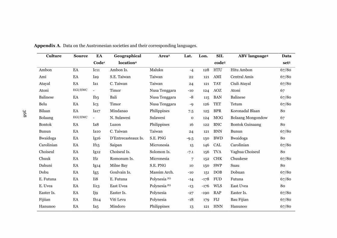
Appendix A. Data on the Austronesian societies and their corresponding languages.
Culture Source EA
Code1
Geographical
location2
Area2 Lat. Lon. SIL
code3
ABV language4 Data
set5
Ambon EA Ic11 Ambon Is. Maluku -4 128 HTU Hitu Ambon 67/80
Ami EA Ia9 S.E. Taiwan Taiwan 22 121 AMI Central Amis 67/80
Atayal EA Ia1 C. Taiwan Taiwan 24 121 TAY Ciuli Atayal 67/80
Atoni EGI/EWC - Timor Nusa Tenggara -10 124 AOZ Atoni 67
Balinese EA Ib3 Bali Nusa Tenggara -8 115 BAN Balinese 67/80
Belu EA Ic3 Timor Nusa Tenggara -9 126 TET Tetum 67/80
Bilaan EA Ia17 Mindanao Philippines 7.5 125 BPR Koronadal Blaan 80
Bolaang EGI/EWC - N. Sulawesi Sulawesi 0 124 MOG Bolaang Mongondow 67
Bontok EA Ia8 Luzon Philippines 16 122 BNC Bontok Guinaang 80
Bunun EA Ia10 C. Taiwan Taiwan 24 121 BNN Bunun 67/80
Bwaidoga EA Ig16 D’Entrecasteaux Is. S.E. PNG -9.5 150 BWD Bwaidoga 80
Carolinian EA If15 Saipan Micronesia 15 146 CAL Carolinian 67/80
Choiseul EA Ig12 Choiseul Is. Solomon Is. -7.1 156 TVA Vaghua Choiseul 80
Chuuk EA If2 Romonum Is. Micronesia 7 152 CHK Chuukese 67/80
Dahuni EA Ig14 Milne Bay S.E. PNG 10 150 SWP Suau 80
Dobu EA Ig5 Goulvain Is. Massim Arch. -10 151 DOB Dobuan 67/80
E. Futuna EA Ii8 E. Futuna Polynesia PO -14 -178 FUD Futuna 67/80
E. Uvea EA Ii13 East Uvea Polynesia PO -13 -176 WLS East Uvea 80
Easter Is. EA Ij9 Easter Is. Polynesia -27 -190 RAP Easter Is. 67/80
Fijiian EA Ih14 Viti Levu Polynesia -18 179 FIJ Bau Fijian 67/80
Hanunoo EA Ia5 Mindoro Philippines 13 121 HNN Hanunoo 67/80
368

Culture Source EA
Code1
Geographical
location2
Area2 Lat. Lon. SIL
code3
ABV language4 Data
set5
Hawaii EA Ij6 Hawaii Polynesia 20 -156 HAW Hawaiian 67/80
Iban EA Ib1 Sarawak Borneo 2 112 IBA Iban 67/80
Ilimandiri EA Ic7 E. Flores Nusa Tenggara -8 123 SLP Lamaholot 67/80
Ilongot EGI/EWC - Luzon Philippines 16 121 ILK Ilongot 67
Javanese EA Ib2 Java Java -7 110 JAV Javanese 67/80
Kaoka EA Ig20 Guadalcanal Solomon Is. -10 160 GRI Ghari Guadalcanal 80
Kapingamarangi EA Ii7 Kapingamarangi Micronesia PO 1 155 KPG Kapingimarangi 80
Kei EA Ic8 Kei Is. Maluku -6 133 KEI Elat Kei Besar 67/80
Kerinci EGI/EWC - Sumatra Sumatra -2 101 KVR Kerinci 67
Kiribati EA If7 Onotoa Is. Micronesia -2 174 GIL Kiribati 67/80
Kodi EA Ic13 Sumba Is. Nusa Tenggara -10 119 KOD Kodi 67/80
Koobe EA Ig17 New Britain Bismarck Arch. -6 151 WIV Vitu 80
Kusaie EA If11 Kosrae Is. Micronesia 5 163 KOS Kusaie 67/80
Kwaio EA Ig18 Malaita Solomon Is. -9 161 KWD Kwaio 67/80
Lakalai EA Ig7 New Britain Bismarck Arch. -5 151 NAK Lakalai 67/80
Lifu EA Ih7 Loyalty Is. New Caledonia -21 167 DHV Dehu 80
Luanguia EA Ii5 Ontong Java Solomon Is. PO -5 160 OJV Luangiua 80
Macassarese EA Ic1 S. Sulawesi Sulawesi -5 119 MAK Makasarese 67/80
Madurese EGI/EWC - Madura Java -7 113 MAD Madurese 67
Malagasy EA Eh2 Madagascar Madagascar -19 46 PLT Merina Malagasy 67/80
Malay EA Ej8 Terengganu Malaysia Pen. 5 103 MSI Malay Bahasa 67/80
Manam EA Ie29 Manam Is. N. PNG -4 145 MVA Manam 67/80
369
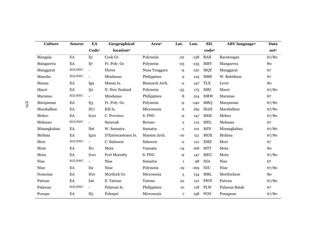
Culture Source EA
Code1
Geographical
location2
Area2 Lat. Lon. SIL
code3
ABV language4 Data
set5
Mangaia EA Ij1 Cook Gr. Polynesia -22 -158 RAR Rarotongan 67/80
Mangareva EA Ij7 Fr. Poly. Gr. Polynesia -23 -135 MRV Mangareva 80
Manggarai EGI/EWC - Flores Nusa Tenggara -9 120 MQY Manggarai 67
Manobo EGI/EWC - Mindanao Philippines 9 125 MBB W. Bukidnon 67
Manus EA Ig9 Manus Is. Bismarck Arch. -2 147 TLX Levei 80
Maori EA Ij2 N. New Zealand Polynesia -35 175 MRI Maori 67/80
Maranao EGI/EWC - Mindanao Philippines 8 124 MRW Maranao 67
Marquesan EA Ij3 Fr. Poly. Gr. Polynesia -9 -140 MRQ Marquesan 67/80
Marshallese EA If17 Kili Is. Micronesia 6 169 MAH Marshallese 67/80
Mekeo EA Ie22 C. Province S. PNG -9 147 MEK Mekeo 67/80
Melanau EGI/EWC - Sarawak Borneo 2 112 MEL Melanau 67
Minangkabau EA Ib6 W. Sumatra Sumatra -1 101 MIN Minangkabau 67/80
Molima EA Ig19 D'Entrecasteaux Is. Massim Arch. -10 151 MOX Molima 67/80
Mori EGI/EWC - C. Sulawesi Sulawesi -2 121 XMZ Mori 67
Mota EA Ih1 Mota Vanuatu -14 168 MTT Mota 80
Motu EA Ie10 Port Moresby S. PNG -9 147 MEU Motu 67/80
Nias EGI/EWC - Nias Sumatra 1 98 NIA Nias 67
Niue EA Ii9 Niue Polynesia -19 -169 NIU Niue 67/80
Nomoian EA If10 Mortlock Gr. Micronesia 5 154 MRL Mortlockese 80
Paiwan EA Ia6 E. Taiwan Taiwan 22 121 PWN Paiwan 67/80
Palawan EGI/EWC - Palawan Is. Philippines 10 118 PLW Palawan Batak 67
Ponape EA If5 Pohnpei Micronesia 7 158 PON Ponapean 67/80
370

Culture Source EA
Code1
Geographical
location2
Area2 Lat. Lon. SIL
code3
ABV language4 Data
set5
Pukapuka EA Ii3 Cook Gr. Polynesia -11 -166 PKP Pukapuka 67/80
Puyuma EA Ia11 E. Taiwan Taiwan 23 121 PYU Puyuma 67/80
Raroian EA Ij5 Tuamotu Gr. Polynesia -16 -142 PMT Tuamotu 80
Rennell EA Ii10 Rennell Is. Solomon Is. PO -12 160 MNV Rennellese 80
Roti EA Ic4 Roti Nusa Tenggara -11 123 TWU Roti Termanu 80
Rotuma EA Ih6 Rotuma Polynesia -13 177 RTM Rotuman 67/80
Samoan EA Ii1 Manua Is. Polynesia -14 -170 SMO Samoan 67/80
Sika EGI/EWC - Flores Nusa Tenggara -9 122 SKI Sika 67
Sugbuhanon EA Ia12 Cebu Philippines 10 124 CEB Cebuano 67/80
Sumbanese EA Ic9 Sumba Is. Nusa Tenggara -10 120 XBR E. Sumbanese Kambera 67/80
Tahiti EA Ij8 Tahiti Polynesia -18 -150 TAH Tahitian 67/80
Tanimbarese EA Ic6 Selaru Is. Nusa Tenggara -8 131 SLU Kei Tanimbar 67/80
Tannese EA Ih10 Tanna Is. Vanuatu -20 168 TNN S.W. Tanna 67/80
Tannga EA Ig21 Tanga (NI) Bismarck Arch. -3 153 TGG Tanga 80
Tikopia EA Ii2 Tikopia Solomon Is. PO -12 168 TKP Tikopia 80
Toba Batak EA Ib4 N. Sumatra Sumatra 2 99 BBC Toba Batak 67/80
Tokelau EA Ii6 Tokelau Polynesia PO -9 -172 TKL Tokelau 80
Tonga EA Ii12 Tongatapu Polynesia -20 -174 TON Tonga 67/80
Tongareva EA Ij10 Cook Gr. Polynesia -9 -158 PNH Penrhyn 80
Toradja EA Ic5 S. Sulawesi Sulawesi -2 121 SDA Tae Toraja 67/80
Trobriand EA Ig2 Trobriand Is. Massim Arch. -8 151 KIJ Kilivila 67/80
Tuvalu EA Ii4 Tuvalu Gr. Polynesia PO -7 179 TVL Tuvalu 80
371

Culture Source EA
Code1
Geographical
location2
Area2 Lat. Lon. SIL
code3
ABV language4 Data
set5
Ulawa EA Ig6 Ulawa Is. Solomon Is. -10 161 APB Sa’a 67/80
Wogeo EA Ie4 Wogeo Is. N. PNG -3 144 WOC Wogeo 80
Woleai EA If4 Woleai Is. Micronesia 7 147 WOE Woleai 67/80
Yami EA Ia14 Orchid Is. Taiwan 22 122 TAO Yami 67/80
Yapese EA If6 Caroline Gr. Micronesia 10 138 YAP Yapese 80
1. Source: EA, Ethnographic Atlas (Murdock 1967); EGI, Ethnic Groups of Island Southeast Asia (LeBar 1975); EWC, Encyclopaedia of
World Cultures (Levinson 1991).
2. Key to geographical areas: Arch., Archipelago; Is. Island; PNG, Papua New Guinea; NG, New Guinea; S., South; E., East; W., West; N.,
North; C., Central; PO, Polynesian Outlier; Nusa Tenggara, Lesser Sunda Is.
3. SIL Code: Summer Institute of Linguistics code for the Ethnologue (http://www.ethnologue.com/).
4. ABV language: Language name in the Austronesian Basic Vocabulary (http://language.psy.auckland.ac.nz/austronesian/)
5. Data set: 67, present in the 67-language data set; 80, present in the 80-language data set; 67/80, language appears in both.
372

Appendix B. Ethnographic Atlas (Murdock 1967) variables recoded into dichotomous categories.
Ethnographic Atlas variable Recoded as: Code Values
Subsistence/ecology variables
Gathering Gathering S1 1 = >6% dependence
0 = 0-5% dependence
Hunting Hunting S2 1 = >6% dependence
0 = 0-5% dependence
Fishing Low dependence on Fishing S3 1 = 0-15% dependence
0 = all others
Moderate dependence on Fishing S4 1 = 16-35% dependence
0 = all others
High dependence on Fishing S5 1 = >36% dependence
0 = all others
Animal Husbandry Low Husbandry S6 1 = 0-5% dependence
0 = all others
Significant Husbandry S7 1 = >16% dependence
0 = all others
Agriculture Low Agriculture S8 1 = 0=45% dependence
0 = all others
Primarily Agriculture S9 1 = >66% dependence
0 = all others
373

Appendix B. (continued)
Ethnographic Atlas variable Recoded as: Code Values
Intensity of Agriculture Extensive or Shifting Agriculture S10 1 = extensive or shifting agriculture
0 = all others
Horticulture S11 1 = horticulture
0 = all others
Intensive Irrigated Agriculture S12 1 = intensive irrigated agriculture
0 = all others
Major Crop Type Tree Fruits S13 1 = tree fruits
0 = all others
Roots/Tubers S14 1 = roots/tubers
0 = all others
Grain S15 1 = cereals grains
0 = all others
Plow Plow absent S16 1 = plow absent
0 = all others
Plow aboriginal S17 1 = plow aboriginal prior to contact
0 = all others
Type of Animal Husbandry Absence of domestics S18 1 = absence or near absence of large domestic animals
0 = all others
Pigs only S19 1 = pigs the only large animals
0 = all others
374
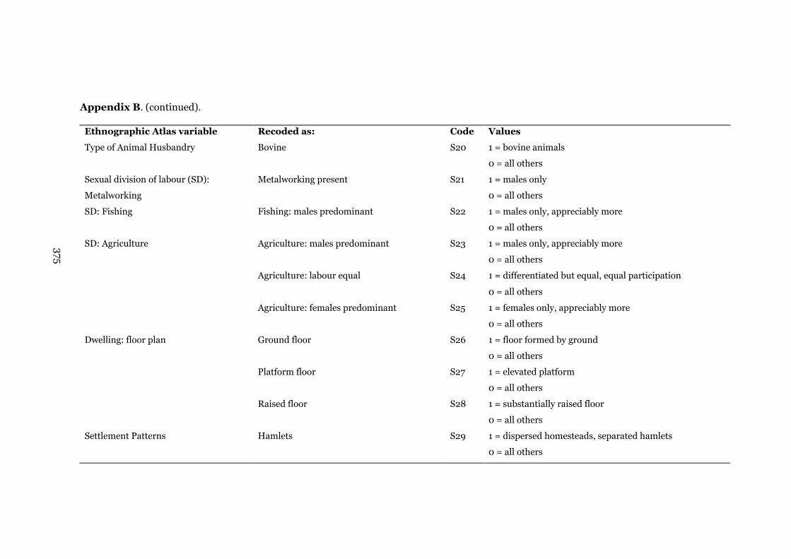
Appendix B. (continued).
Ethnographic Atlas variable Recoded as: Code Values
Type of Animal Husbandry Bovine S20 1 = bovine animals
0 = all others
Sexual division of labour (SD):
Metalworking
Metalworking present S21 1 = males only
0 = all others
SD: Fishing Fishing: males predominant S22 1 = males only, appreciably more
0 = all others
SD: Agriculture Agriculture: males predominant S23 1 = males only, appreciably more
0 = all others
Agriculture: labour equal S24 1 = differentiated but equal, equal participation
0 = all others
Agriculture: females predominant S25 1 = females only, appreciably more
0 = all others
Dwelling: floor plan Ground floor S26 1 = floor formed by ground
0 = all others
Platform floor S27 1 = elevated platform
0 = all others
Raised floor S28 1 = substantially raised floor
0 = all others
Settlement Patterns Hamlets S29 1 = dispersed homesteads, separated hamlets
0 = all others
375

Appendix B. (continued).
Ethnographic Atlas variable Recoded as: Code Values
Settlement Patterns Compact S30 1 = compact relatively permanent, complex settlements
0 = all others
Kinship variables
Primary mode of marriage Brideprice K1 1 = brideprice, -wealth, -service, token brideprice
0 = all others
Gift exchange K2 1 = reciprocal gift exchange
0 = all others
No consideration of marriage transactions K3 1 = absence of consideration
0 = all others
Domestic organisation Monogamous nuclear family K4 1 = independent monogamous nuclear family
0 = all others
Polygyny K5 1 = all polygynous forms
0 = all others
Extended families K6 1 = minimal, small & large extended families
0 = all others
Monogamy and Polygamy Monogamy K7 1 = monogamous
0 = all others
Polygamy K8 1 = all polygamous forms
0 = all others
376
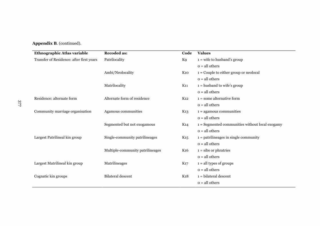
Appendix B. (continued).
Ethnographic Atlas variable Recoded as: Code Values
Transfer of Residence: after first years Patrilocality K9 1 = wife to husband’s group
0 = all others
Ambi/Neolocality K10 1 = Couple to either group or neolocal
0 = all others
Matrilocality K11 1 = husband to wife’s group
0 = all others
Residence: alternate form Alternate form of residence K12 1 = some alternative form
0 = all others
Community marriage organisation Agamous communities K13 1 = agamous communities
0 = all others
Segmented but not exogamous K14 1 = Segmented communities without local exogamy
0 = all others
Largest Patrilineal kin group Single-community patrilineages K15 1 = patrilineages in single community
0 = all others
Multiple-community patrilineages K16 1 = sibs or phratries
0 = all others
Largest Matrilineal kin group Matrilineages K17 1 = all types of groups
0 = all others
Cognatic kin groups Bilateral descent K18 1 = bilateral descent
0 = all others
377
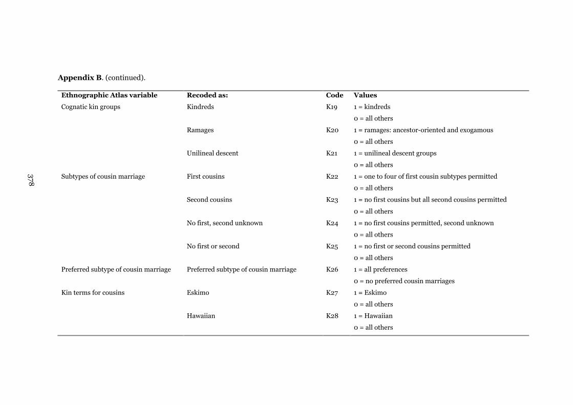
Appendix B. (continued).
Ethnographic Atlas variable Recoded as: Code Values
Cognatic kin groups Kindreds K19 1 = kindreds
0 = all others
Ramages K20 1 = ramages: ancestor-oriented and exogamous
0 = all others
Unilineal descent K21 1 = unilineal descent groups
0 = all others
Subtypes of cousin marriage First cousins K22 1 = one to four of first cousin subtypes permitted
0 = all others
Second cousins K23 1 = no first cousins but all second cousins permitted
0 = all others
No first, second unknown K24 1 = no first cousins permitted, second unknown
0 = all others
No first or second K25 1 = no first or second cousins permitted
0 = all others
Preferred subtype of cousin marriage Preferred subtype of cousin marriage K26 1 = all preferences
0 = no preferred cousin marriages
Kin terms for cousins Eskimo K27 1 = Eskimo
0 = all others
Hawaiian K28 1 = Hawaiian
0 = all others
378

Appendix B. (continued).
Ethnographic Atlas variable Recoded as: Code Values
Kin terms for cousins Iroquois K29 1 = Iroquois
0 = all others
Descent Patrilineal K30 1 = patrilineal
0 = all others
Matrilineal K31 1 = matrilineal
0 = all others
Ambilineal K32 1 = ambilineal
0 = all others
Bilateral K33 1 = bilateral
0 = all others
Mixed K34 1 = mixed, duolateral
0 = all others
Political
Community hierarchy Three levels of community hierarchy P1 1 = three levels of community hierarchy
0 = all others
Four levels of community hierarchy P2 1 = four levels of community hierarchy
0 = all others
Beyond-community hierarchy None P3 1 = no levels beyond community
0 = all others
379

Appendix B. (continued).
Ethnographic Atlas variable Recoded as: Code Values
Beyond-community hierarchy One P4 1 = one level beyond community
0 = all others
Two or more P5 1 = two or more levels beyond community
0 = all others
Class stratification No classes P6 1 = absence among freemen
0 = all others
Wealth distinctions P7 1 = wealth distinctions
0 = all others
Elaborated class distinction P8 1 = elite, dual, complex classes
0 = all others
Type of slavery Slavery P9 1 = any type present
0 = all others
Former presence of slavery Former slavery P10 1 = formerly present but not current
0 = all others
Succession to office of headman Hereditary succession P11 1 = patrilineal, matrilineal heir
0 = all others
Non-hereditary succession P12 1 = appointment, seniority, consensus, influence
0 = all others
380