a comparative study for design of boundary combined

Coupled Systems Mechanics, Vol. 6, No. 4 (2017) 417-437

DOI: https://doi.org/10.12989/csm.2017.6.4.417 417

Copyright © 2017 Techno-Press, Ltd. http://www.techno-press.org/?journal=csm&subpage=8 ISSN: 2234-2184 (Print), 2234-2192 (Online)

A comparative study for design of boundary combined footings of trapezoidal and rectangular forms using new

models

Arnulfo Luévanos-Rojas*1, José Daniel Barquero-Cabrero2a, Sandra López-Chavarría1b and Manuel Medina-Elizondo1c

1Institute of Multidisciplinary Researches, Autonomous University of Coahuila,

Blvd. Revolución No, 151 Ote, CP 27000, Torreón, Coahuila, México 2Institute for Long Life Learning IL3, University of Barcelona,

Street Girona No, 24, CP 08010, Barcelona, Spain

(Received April 27, 2017, Revised August 23, 2017, Accepted August 24, 2017)

Abstract. This paper shows a comparative study for design of reinforced concrete boundary combined

footings of trapezoidal and rectangular forms supporting two columns and each column transmits an axial

load and a moment around of the axis X (transverse axis of the footing) and other moment around of the axis

Y (longitudinal axis of the footing) to foundation to obtain the most economical combined footing. The real

soil pressure acting on the contact surface of the footings is assumed as a linear variation. Methodology used

to obtain the dimensions of the footings for the two models consider that the axis X of the footing is located

in the same position of the resultant, i.e., the dimensions is obtained from the position of the resultant. The

main part of this research is to present the differences between the two models. Results show that the

trapezoidal combined footing is more economical compared to the rectangular combined footing. Therefore,

the new model for the design of trapezoidal combined footings should be used, and complies with real

conditions.

Keywords: design of trapezoidal combined footings; design of rectangular combined footings; bending

moments; bending shear; punching shear

1. Introduction

Footings are structural elements that transmit column or wall loads to the underlying soil below

the structure. Footings are designed to transmit these loads to the soil without exceeding its safe

bearing capacity, to prevent excessive settlement of the structure to a tolerable limit, to minimize

differential settlement, and to prevent sliding and overturning. The choice of suitable type of

Corresponding author, Ph.D., E-mail: [email protected] aPh.D., E-mail: [email protected] bPh.D., E-mail: [email protected] cPh.D., E-mail: [email protected]

mailto:[email protected]




Arnulfo Luévanos-Rojas et al.

footing depends on the depth at which the bearing stratum is localized, the soil condition and the

type of superstructure. The foundations are classified into superficial and deep, which have

important differences: in terms of geometry, the behavior of the soil, its structural functionality and

its constructive systems (Bowles 2001, Das et al. 2006).

The design of superficial solution is done for the following load cases: 1) the footings subjected

to concentric axial load, 2) the footings subjected to axial load and moment in one direction

(uniaxial bending), 3) the footings subjected to axial load and moment in two directions (biaxial

bending) (Bowles 2001, Das et al. 2006, Calabera 2000, Tomlinson 2008, McCormac and Brown

2013, González-Cuevas and Robles-Fernandez-Villegas 2005).

Superficial foundations may be of various types according to their function; isolated footing,

combined footing, strip footing, or mat foundation (Bowles 2001).

A combined footing is a long footing supporting two or more columns in (typically two) one

row. The combined footing may be rectangular, trapezoidal or T-shaped in plan. Rectangular

footing is provided when one of the projections of the footing is restricted or the width of the

footing is restricted. Trapezoidal footing or T-shaped is provided when one column load is much

more than the other. As a result, both projections of the footing beyond the faces of the columns

will be restricted (Kurian 2005, Punmia et al. 2007, Varghese 2009).

The distribution of soil pressure under a footing is a function of the type of soil, the relative

rigidity of the soil and the footing, and the depth of foundation at level of contact between footing

and soil. A concrete footing on sand will have a pressure distribution similar to Fig. 1(a). A

concrete footing on clay will have a pressure distribution similar to Fig. 1(b). As the footing is

loaded, the soil under the footing deflects in a bowl-shaped depression, relieving the pressure

under the middle of the footing. For design purposes, it is common to assume the soil pressure is

linearly distributed. The pressure distribution will be uniform if the centroid of the footing

coincides with the resultant of the applied loads, as shown in Fig. 1(c) (Bowles 2001).

Fig. 1 Pressure distribution under footing; (a) footing on sand; (b) footing on clay; (c) equivalent uniform

distribution

Construction practice may dictate using only one footing for two or more columns due to:

a) Closeness of column (for example around elevator shafts and escalators).

b) To property line constraint, this may limit the size of footings at boundary. The eccentricity

of a column placed on an edge of a footing may be compensated by tying the footing to the interior

column.

Conventional method for design of combined footings by rigid method assumes that (Bowles

2001, Das et al. 2006, McCormac and Brown 2013, González-Cuevas and Robles-Fernandez-

Villegas 2005):

1. The footing or mat is infinitely rigid, and therefore, the deflection of the footing or mat does

418

A comparative study for design of boundary combined footings…

not influence the pressure distribution.

2. The soil pressure is linearly distributed or the pressure distribution will be uniform, if the

centroid of the footing coincides with the resultant of the applied loads acting on foundations.

3. The minimum stress should be equal to or greater than zero, because the soil is not capable

of withstand tensile stresses.

4. The maximum stress must be equal or less than the allowable capacity that can withstand the

soil.

Some papers presents the equations to obtain the dimension of footings are: A mathematical

model for dimensioning of rectangular footings (Luévanos-Rojas 2013); A mathematical model for

dimensioning of square footings (Luévanos-Rojas 2012a); A mathematical model for the

dimensioning of circular footings (Luévanos-Rojas 2012b); A new mathematical model for

dimensioning of the boundary trapezoidal combined footings (Luévanos-Rojas 2015a); A

mathematical model for the dimensioning of rectangular combined footings (Luévanos-Rojas

2016a); Optimal dimensioning for the corner combined footings (López-Chavarría et al. 2017).

Guler and Celep (2005) presented the response of a rectangular plate-column system on a

tensionless winkler foundation subjected to static and dynamic loads.

Chen et al. (2011) investigated the nonlinear vibration behavior for a hybrid composite plate

subjected to initial stresses on elastic foundations to obtain the nonlinear partial differential

equations of motion.

Smith-Pardo (2011) showed a study on a performance-based framework for soil-structure

systems using simplified rocking foundation models.

Shahin and Cheung (2011) presented the stochastic design charts for bearing capacity of strip

footings.

Zhang et al. (2011) showed a nonlinear analysis of finite beam resting on winkler with

consideration of beam-soil interface resistance effect.

Agrawal and Hora (2012) presented a nonlinear interaction behavior of infilled frame-isolated

footings-soil system subjected to seismic loading.

Rad (2012) realized the study on the static behavior of bi-directional functionally graded (FG)

non-uniform thickness circular plate resting on quadratically gradient elastic foundations (Winkler-

Pasternak type) subjected to axisymmetric transverse and in-plane shear efforts is carried out by

using a model 3D and differential quadrature methods.

Maheshwari and Khatri (2012) estimated the influence of inclusion of geosynthetic layer on

response of combined footings on stone column of earth beds reinforced.

Orbanich et al. (2012) showed a study on strenghtening and repair of concrete foundation

beams with fiber composite materials.

Mohamed et al. (2013) presented the generalized schmertmann equation for settlement

estimation of shallow footings in saturated and unsaturated sands.

Luévanos-Rojas et al. (2013) proposed a design of isolated footings of rectangular form using a

new model.

Orbanich and Ortega (2013) this study aimed to investigate the mechanical behavior of

rectangular foundation plates with perimetric beams and internal stiffening beams of the plate is

herein analyzed, taking the foundation design into account.

Dixit and Patil (2013) showed an experimental estimate of Nγ values and corresponding

settlements for square footings on finite layer of sand.

ErzÍn and Gul (2013) presented the use of neural networks for the prediction of the settlement

of pad footings on cohesionless soils based on standard penetration test.

419


Cure et al. (2014) proposed the decrease trends of ultimate loads of eccentrically loaded model

strip footings close to a slope.

Luévanos-Rojas (2014a) presented a design of isolated footings of circular form using a new

model.

Luévanos-Rojas (2014b) proposed a design of boundary combined footings of rectangular

shape using a new model.

Uncuoğlu (2015) showed a study on bearing capacity of square footings on sand layer

overlying clay.

Luévanos-Rojas (2015b) presented a design of boundary combined footings of trapezoidal form

using a new model.

Luévanos-Rojas (2016b) showed a comparative study for the design of rectangular and circular

isolated footings using new models.

Luévanos-Rojas (2016c) proposed a new model for design of boundary rectangular combined

footings with two opposite sides restricted.

This paper shows a comparative study for design of reinforced concrete boundary combined

footings of trapezoidal and rectangular forms supporting two columns and each column transmits

an axial load and a moment around of the axis X (transverse axis of the footing) and other moment

around of the axis Y (longitudinal axis of the footing) to foundation to obtain the most economical

combined footing. The real soil pressure acting on the contact surface of the footings is assumed as

a linear variation. Methodology used to obtain the dimensions of the footings for the two models

consider that the axis X of the footing is located in the same position of the resultant, i.e., the

dimensions of the footings is obtained from the position of the resultant. The main part of this

research is to present the differences between the two models.

2. Formulation of the new models

2.1 Boundary trapezoidal combined footings

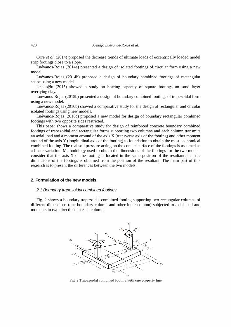
Fig. 2 shows a boundary trapezoidal combined footing supporting two rectangular columns of

different dimensions (one boundary column and other inner column) subjected to axial load and

moments in two directions in each column.

Fig. 2 Trapezoidal combined footing with one property line

420


The value of “Cy1” is obtained by the equation (Luévanos-Rojas 2015a)

𝐶𝑦1 =𝑅𝑐1 + 2𝑃2𝐿 − 2𝑀𝑥𝑇

2𝑅 (1)

where: R=P1+P2 and MxT=Mx1+Mx2.

The value of “a” must comply with the following (Luévanos-Rojas 2015a)

3

2𝐶𝑦1 < 𝑎 < 3𝐶𝑦1 (2)

If the trapezoidal combined footing has two property lines in opposite ends. The value of “a” is

(Luévanos-Rojas 2015a)

𝑎 =𝑐1

2+ 𝐿 +

𝑐3

2 (3)

The value of “b2” is found as follows. If the soil pressure is considered equal to zero, the value

of “b2” is obtained by the following equation (Luévanos-Rojas 2015a)

𝑏2 =12𝑀𝑦𝑇(2𝑎 − 3𝐶𝑦1)(3𝐶𝑦1 − 𝑎)

𝑅(5𝑎2 − 18𝑎𝐶𝑦1 + 18𝐶𝑦12)

(4)

where: MyT=My1+My2.

Now, if the soil pressure is considered available load capacity “σadm”, the value of “b2” is

obtained by the following equation (Luévanos-Rojas 2015a)

𝜎𝑎𝑑𝑚𝑎2(5𝑎2 − 18𝑎𝐶𝑦1 + 18𝐶𝑦12)𝑏2

2 − 2𝑅(3𝐶𝑦1 − 𝑎)(5𝑎2 − 18𝑎𝐶𝑦1 + 18𝐶𝑦12)𝑏2

− 24𝑀𝑦𝑇(2𝑎 − 3𝐶𝑦1)(3𝐶𝑦1 − 𝑎)2

= 0 (5)

The greater value obtained by Eqs. (4)-(5) is the value considered for “b2”.

Once known the value of “b2” is substituted into following equation to obtain the value of “b1”

(Luévanos-Rojas 2015a)

𝑏1 = (2𝑎 − 3𝐶𝑦1

3𝐶𝑦1 − 𝑎) 𝑏2 (6)

2.1.1 Moments Critical sections for moments are presented in section a1’-a1’, a2’-a2’, b’-b’, c’-c’, d’-d’ and e’-

e’, as shown in Fig. 3.

Fig. 3 Critical sections for moments

421


2.1.1.1 Moment around of the axis a1’-a1’ The moment around of the axis a1’-a1’ is obtained using the following equation (Luévanos-

Rojas 2015b)

𝑀𝑎1= [𝑃1𝑎(𝑏1

2 + 𝑏112){3𝑎2(𝑏1 − 𝑐2)2 − 3𝑎𝑤1(𝑏1 − 𝑏2)(𝑏1 − 𝑐2) + 𝑤1

2(𝑏1 − 𝑏2)2}

+ 6𝑀𝑦1{2𝑎3(2𝑏13 − 3𝑏1

2𝑐2 + 𝑐23) − 6𝑎2𝑏1𝑤1(𝑏1 − 𝑏2)(𝑏1 − 𝑐2)

+ 2𝑎𝑤12(𝑏1 − 𝑏2)2(2𝑏1 − 𝑐2) − 𝑤1

3(𝑏1 − 𝑏2)3}]

/[12𝑎3(𝑏1 + 𝑏11)(𝑏12 + 𝑏11

2)]

(7)


Rojas 2015b)

𝑀𝑎2= [𝑃2𝑎(𝑏21

2 + 𝑏222){3[2𝑎(𝑏1 − 𝑐4) − (𝑏1 − 𝑏2)(2𝐿 + 𝑐1)]2 + 𝑤2

2(𝑏1 − 𝑏2)2}

+ 12𝑀𝑦2{4𝑎3(𝑏1 − 𝑐4)2(2𝑏1 + 𝑐4) − 12𝑎2𝑏1(𝑏1 − 𝑐4)(𝑏1 − 𝑏2)(2𝐿 + 𝑐1)

+ 𝑎(𝑏1 − 𝑏2)2(2𝑏1 − 𝑐4)[3(2𝐿 + 𝑐1)2 + 𝑤22]

− (𝑏1 − 𝑏2)3[(2𝐿 + 𝑐1)3 + 𝑤22(2𝐿 + 𝑐1)]}]

/[48𝑎3(𝑏21 + 𝑏22)(𝑏212 + 𝑏22

2)]

(8)

where: w1 = c1+d/2, w2 = c3+d, b11 = b1 – w1(b1–b2)/a, b21 = b1 – (c1+2L–w2)(b1–b2)/2a, b22 = b1 –

(c1+2L+w2)(b1–b2)/2a.

2.1.1.3 Moment around of the axis b’-b’ The moment around of the axis b’-b’ is (Luévanos-Rojas 2015b)

𝑀𝑏 =𝑃1𝑐1

2−

𝑅𝑐12[3𝑎𝑏1 − 𝑐1(𝑏1 − 𝑏2)]

3𝑎2(𝑏1 + 𝑏2)+ 𝑀𝑥1 (9)

2.1.1.4 Moment around of the axis c’-c’ The maximum moment is presented on the axis c’-c’, and shear force is zero. Then the shear

force is obtained at a distance “ym”, and must be equal to zero. The equation to obtain “ym” is

shown as follows (Luévanos-Rojas 2015b)

𝑦𝑚 =𝑎√𝑅[𝑏1

2(𝑅 − 𝑃1) + 𝑃1𝑏22] − 𝑅(𝐶𝑦1𝑏2 + 𝐶𝑦2𝑏1)

𝑅(𝑏1 − 𝑏2)

(10)

The moment around of the axis c’-c’ is obtained using the following equation (Luévanos-Rojas

2015b)

𝑀𝑐 = 𝑃1 (𝐶𝑦1 −𝑐1

2− 𝑦𝑚) −

𝑅(𝐶𝑦1 − 𝑦𝑚)[2𝑎𝑏2 + (𝑏1 − 𝑏2)(2𝐶𝑦2 + 𝐶𝑦1 + 𝑦𝑚)](𝑦𝑐𝑐 − 𝑦𝑚)

𝑎2(𝑏1 + 𝑏2)+ 𝑀𝑥1

(11)

422


where: ycc is the gravity center of the soil pressure the area formed by the axis c’-c’ and the corners

1 and 2 with respect the axis “X”, and this is obtained by the following equation (Luévanos-Rojas

2015b)

𝑦𝑐𝑐 =(𝑏1 − 𝑏2)(𝐶𝑦1 − 𝑦𝑚)

2

6[2𝑎𝑏2 + (𝑏1 − 𝑏2)(2𝐶𝑦2 + 𝐶𝑦1 + 𝑦𝑚)]+

𝐶𝑦1

2+

𝑦𝑚

2 (12)

2.1.1.5 Moment around of the axis d’-d’ The moment around of the axis d’-d’ is obtained using the following equation (Luévanos-Rojas

2015b)

𝑀𝑑 = 𝑃1 (𝐿 −𝑐3

2) −

𝑅(2𝐿 − 𝑐3 + 𝑐1)2[6𝑎𝑏1 − (𝑏1 − 𝑏2)(2𝐿 − 𝑐3 + 𝑐1)]

24𝑎2(𝑏1 + 𝑏2)+ 𝑀𝑥1 (13)

2.1.1.6 Moment around of the axis e’-e’ The moment around of the axis e’-e’ is obtained as follows (Luévanos-Rojas 2015b)

𝑀𝑒 = 𝑃1 (𝐿 +𝑐3

2) + 𝑃2 (

𝑐3

2) −

𝑅(2𝐿 + 𝑐3 + 𝑐1)2[6𝑎𝑏1 − (𝑏1 − 𝑏2)(2𝐿 + 𝑐3 + 𝑐1)]

24𝑎2(𝑏1 + 𝑏2)+ 𝑀𝑥1

+ 𝑀𝑥2 (14)

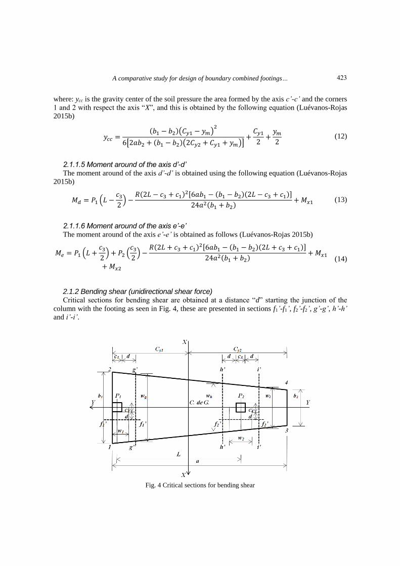
2.1.2 Bending shear (unidirectional shear force) Critical sections for bending shear are obtained at a distance “d” starting the junction of the

column with the footing as seen in Fig. 4, these are presented in sections f1’-f1’, f2’-f2’, g’-g’, h’-h’

and i’-i’.

Fig. 4 Critical sections for bending shear

423


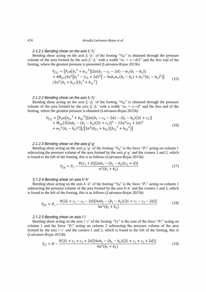
2.1.2.1 Bending shear on the axis f1’-f1’ Bending shear acting on the axis f1’-f1’ of the footing “Vff1” is obtained through the pressure

volume of the area formed by the axis f1’-f1’ with a width “w1 = c1+d/2” and the free end of the

footing, where the greatest pressure is presented (Luévanos-Rojas 2015b)

𝑉𝑓𝑓1= [𝑃1𝑎(𝑏1

2 + 𝑏112)[2𝑎(𝑏1 − 𝑐2 − 2𝑑) − 𝑤1(𝑏1 − 𝑏2)]

+ 4𝑀𝑦1{3𝑎2[𝑏12 − (𝑐2 + 2𝑑)2] − 3𝑎𝑏1𝑤1(𝑏1 − 𝑏2) + 𝑤1

2(𝑏1 − 𝑏2)2}]

/2𝑎2(𝑏1 + 𝑏11)(𝑏12 + 𝑏11

2) (15)

2.1.2.2 Bending shear on the axis f2’-f2’ Bending shear acting on the axis f2’-f2’ of the footing “Vff2” is obtained through the pressure

volume of the area formed by the axis f2’-f2’ with a width “w2 = c3+d” and the free end of the

footing, where the greatest pressure is obtained (Luévanos-Rojas 2015b)

𝑉𝑓𝑓2= [𝑃2𝑎(𝑏21

2 + 𝑏222)[2𝑎(𝑏1 − 𝑐4 − 2𝑑) − (𝑏1 − 𝑏2)(2𝐿 + 𝑐1)]

+ 𝑀𝑦2{3[2𝑎𝑏1 − (𝑏1 − 𝑏2)(2𝐿 + 𝑐1)]2 − 12𝑎2(𝑐4 + 2𝑑)2

+ 𝑤22(𝑏1 − 𝑏2)2}]/[2𝑎2(𝑏21 + 𝑏22)(𝑏21

2 + 𝑏222)]

(16)

2.1.2.3 Bending shear on the axis g’-g’ Bending shear acting on the axis g’-g’ of the footing “Vfg” is the force “P1” acting on column 1

subtracting the pressure volume of the area formed by the axis g'-g’ and the corners 1 and 2, which

is found to the left of the footing, this is as follows (Luévanos-Rojas 2015b)

𝑉𝑓𝑔 = 𝑃1 −𝑅(𝑐1 + 𝑑)[2𝑎𝑏1 − (𝑏1 − 𝑏2)(𝑐1 + 𝑑)]

𝑎2(𝑏1 + 𝑏2) (17)

2.1.2.4 Bending shear on axis h’-h’ Bending shear acting on the axis h’-h’ of the footing “Vfh” is the force “P1” acting on column 1

subtracting the pressure volume of the area formed by the axis h'-h’ and the corners 1 and 2, which

is found to the left of the footing, this is as follows (Luévanos-Rojas 2015b)

𝑉𝑓ℎ = 𝑃1 −𝑅(2𝐿 + 𝑐1 − 𝑐3 − 2𝑑)[4𝑎𝑏1 − (𝑏1 − 𝑏2)(2𝐿 + 𝑐1 − 𝑐3 − 2𝑑)]

4𝑎2(𝑏1 + 𝑏2) (18)

2.1.2.5 Bending shear on axis i’-i’ Bending shear acting on the axis i’-i’ of the footing “Vfi” is the sum of the force “P1” acting on

column 1 and the force “P2” acting on column 2 subtracting the pressure volume of the area

formed by the axis i’-i’ and the corners 1 and 2, which is found to the left of the footing, this is

(Luévanos-Rojas 2015b)

𝑉𝑓𝑖 = 𝑅 −𝑅(2𝐿 + 𝑐1 + 𝑐3 + 2𝑑)[4𝑎𝑏1 − (𝑏1 − 𝑏2)(2𝐿 + 𝑐1 + 𝑐3 + 2𝑑)]

4𝑎2(𝑏1 + 𝑏2) (19)

424


2.1.3 Punching shear (bidirectional shear force) Critical section for the punching shear appears at a distance “d/2” starting the junction of the

column with the footing in the two directions, as shown in Fig. 5.

Fig. 5 Critical sections for punching shear

2.1.3.1 Punching shear for boundary column Critical section for the punching shear is presented in rectangular section formed by points 5, 6, 7

and 8. Punching shear acting on the footing “Vp1” is the force “P1” acting on column 1 subtracting

the pressure volume of the area formed by point’s 5, 6, 7 and 8 (Luévanos-Rojas 2015b)

𝑉𝑝1 = 𝑃1 −𝑅(2𝑐1 + 𝑑)(𝑐2 + 𝑑)

𝑎(𝑏1 + 𝑏2) (20)

2.1.3.2 Punching shear for inner column Critical section for the punching shear is presented in rectangular section formed by points 9,

10, 11 and 12. Punching shear acting on the footing “Vp2” is the force “P2” acting on column 2

subtracting the pressure volume of the area formed by the point’s 9, 10, 11 and 12 (Luévanos-

Rojas 2015b)

𝑉𝑝2 = 𝑃2 −2𝑅(𝑐3 + 𝑑)(𝑐4 + 𝑑)

𝑎(𝑏1 + 𝑏2) (21)

2.2 Boundary rectangular combined footings

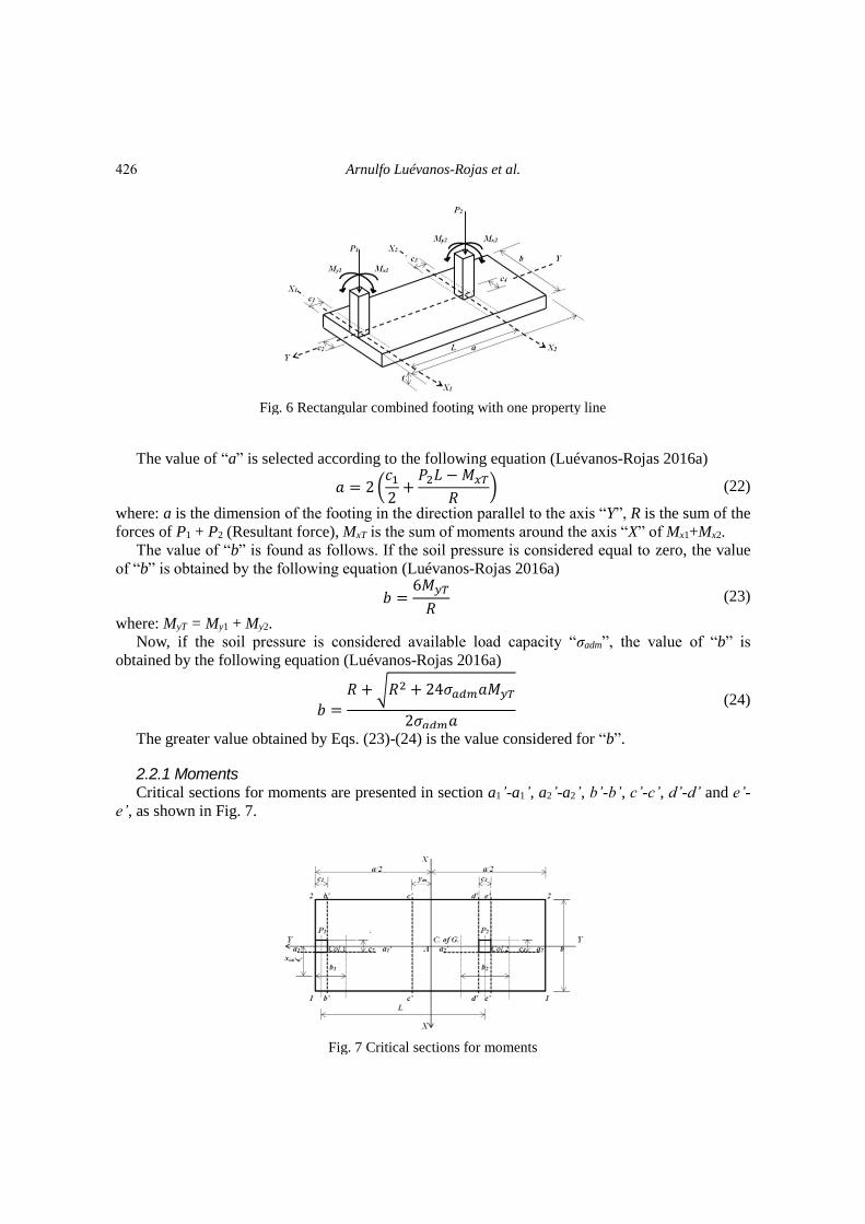
Fig. 6 shows a combined footing supporting two rectangular columns of different dimensions (a

boundary column and other inner column) subject to axial load and moments in two directions

(bidirectional bending) each column.

425


Fig. 6 Rectangular combined footing with one property line

The value of “a” is selected according to the following equation (Luévanos-Rojas 2016a)

𝑎 = 2 (𝑐1

2+

𝑃2𝐿 − 𝑀𝑥𝑇

𝑅) (22)

where: a is the dimension of the footing in the direction parallel to the axis “Y”, R is the sum of the

forces of P1 + P2 (Resultant force), MxT is the sum of moments around the axis “X” of Mx1+Mx2.

The value of “b” is found as follows. If the soil pressure is considered equal to zero, the value

of “b” is obtained by the following equation (Luévanos-Rojas 2016a)

𝑏 =6𝑀𝑦𝑇

𝑅 (23)

where: MyT = My1 + My2.

Now, if the soil pressure is considered available load capacity “σadm”, the value of “b” is

obtained by the following equation (Luévanos-Rojas 2016a)

𝑏 =

𝑅 + √𝑅2 + 24𝜎𝑎𝑑𝑚𝑎𝑀𝑦𝑇

2𝜎𝑎𝑑𝑚𝑎

(24)

The greater value obtained by Eqs. (23)-(24) is the value considered for “b”.

2.2.1 Moments Critical sections for moments are presented in section a1’-a1’, a2’-a2’, b’-b’, c’-c’, d’-d’ and e’-

e’, as shown in Fig. 7.

Fig. 7 Critical sections for moments

426



Rojas 2014b)

𝑀𝑎1=

(𝑏 − 𝑐2)2[𝑃1𝑏2 + 2𝑀𝑦1(2𝑏 + 𝑐2)]

8𝑏3 (25)


Rojas 2014b)

𝑀𝑎2=

(𝑏 − 𝑐4)2[𝑃2𝑏2 + 2𝑀𝑦2(2𝑏 + 𝑐4)]

8𝑏3 (26)

2.2.1.3 Moment around of the axis b’-b’ The moment around of the axis b’-b’ is obtained using the following equation (Luévanos-Rojas

2014b)

𝑀𝑏 = (𝑃1 −𝑅𝑐1

𝑎)

𝑐1

2+ 𝑀𝑥1 (27)

2.2.1.4 Moment around of the axis c’-c’ The maximum moment is presented on the axis c’-c’, and shear force is zero. Then the shear

force is obtained at a distance “ym”, and must be equal to zero. The equation to obtain “ym” is

shown as follows (Luévanos-Rojas 2014b)

𝑦𝑚 =𝑎

2−

𝑃1𝑎

𝑅 (28)

The moment around of the axis c’-c’ is obtained using the following equation (Luévanos-Rojas

2014b)

𝑀𝑐 =𝑃1(𝑃1𝑎 − 𝑅𝑐1)

2𝑅+ 𝑀𝑥1 (29)

2.2.1.5 Moment around of the axis d’-d’ The moment around of the axis d’-d’ is obtained using the following equation (Luévanos-Rojas

2014b)

𝑀𝑑 = 𝑃1 (𝐿 −𝑐3

2) −

𝑅

2𝑎(𝐿 +

𝑐1 − 𝑐3

2)

2

+ 𝑀𝑥1 (30)

2.2.1.6 Moment around of the axis e’-e’ The moment around of the axis e’-e’ is obtained using the following equation (Luévanos-Rojas

2014b)

𝑀𝑒 = 𝑃1𝐿 +𝑅𝑐3

2−

𝑅

2𝑎(𝐿 +

𝑐1 + 𝑐3

2)

2

+ 𝑀𝑥1 + 𝑀𝑥2 (31)

427


2.2.2 Bending shear (unidirectional shear force) The critical sections for bending shear are obtained at a distance “d” starting the junction of the

column with the footing as seen in Fig. 8, these are presented in sections f1’-f1’, f2’-f2’, g’-g’, h’-h’

and i’-i’.

Fig. 8 Critical sections for bending shear

2.2.2.1 Bending shear on the axis f1’-f1’ Bending shear acting on the axis f1’-f1’ of the footing “Vff1” is obtained through of the volume

of pressure of the area formed by the axis f1’-f1’ with a width “b1 = c1+d/2” and the free end of the

rectangular footing, where the greatest pressure is presented (Luévanos-Rojas 2014b)

𝑉𝑓𝑓1=

𝑃1(𝑏 − 𝑐2 − 2𝑑)

2𝑏+

3𝑀𝑦1[𝑏2 − (𝑐2 + 2𝑑)2]

2𝑏3 (32)

2.2.2.2 Bending shear on the axis f2’-f2’ Bending shear acting on the axis f2’-f2’ of the footing “Vff2” is obtained through of the volume

of pressure of the area formed by the axis f2’-f2’ with a width “b2 = c3+d” and the free end of the

rectangular footing, where the greatest pressure is presented (Luévanos-Rojas 2014b)

𝑉𝑓𝑓2=

𝑃2(𝑏 − 𝑐4 − 2𝑑)

2𝑏+

3𝑀𝑦2[𝑏2 − (𝑐4 + 2𝑑)2]

2𝑏3 (33)

2.2.2.3 Bending shear on the axis g’-g’ Bending shear acting on the axis g’-g’ of the footing “Vfg” is obtained through of the volume of

pressure of the area formed by the axis g’-g’ and the corners 1 and 2 to the left of the footing, this

is as follows (Luévanos-Rojas 2014b)

𝑉𝑓𝑔′ = 𝑃1 −𝑅(𝑐1 + 𝑑)

𝑎 (34)

428


2.2.2.4 Bending shear on the axis h’-h’ Bending shear acting on the axis h’-h’ of the footing “Vfh” is the force “P1” acting in column 1

less the volume of pressure of the area formed by the axis h’-h’ and the corners 1 and 2, which is

found to the left of the footing, this is as follows (Luévanos-Rojas 2014b)

𝑉𝑓ℎ′ = 𝑃1 −𝑅

𝑎(𝐿 +

𝑐1 − 𝑐3

2− 𝑑) (35)

2.2.2.5 Bending shear on the axis i’-i’ Bending shear acting on the axis i’-i’ of the footing “Vfi” is the sum of the force “P1” acting on

column 1 and the force “P2” acting on column 2 less the volume of pressure of the area formed by

the axis i’-i’ and the corners 1 and 2, which is found to the left of the footing, this is as follows

(Luévanos-Rojas 2014b)

𝑉𝑓𝑖′ = 𝑅 −𝑅

𝑎(𝐿 +

𝑐1 + 𝑐3

2+ 𝑑) (36)

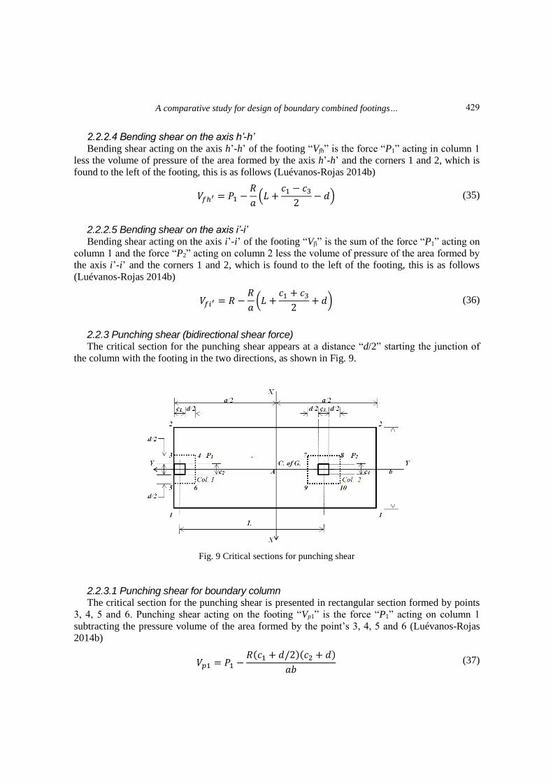
2.2.3 Punching shear (bidirectional shear force) The critical section for the punching shear appears at a distance “d/2” starting the junction of

the column with the footing in the two directions, as shown in Fig. 9.

Fig. 9 Critical sections for punching shear

2.2.3.1 Punching shear for boundary column The critical section for the punching shear is presented in rectangular section formed by points

3, 4, 5 and 6. Punching shear acting on the footing “Vp1” is the force “P1” acting on column 1

subtracting the pressure volume of the area formed by the point’s 3, 4, 5 and 6 (Luévanos-Rojas

2014b)

𝑉𝑝1 = 𝑃1 −𝑅(𝑐1 + 𝑑/2)(𝑐2 + 𝑑)

𝑎𝑏 (37)

429


2.2.3.2 Punching shear for inner column The critical section for the punching shear is presented in rectangular section formed by points

7, 8, 9 and 10. Punching shear acting on the footing “Vp2” is the force “P2” acting on column 2

subtracting the pressure volume of the area formed by the point’s 7, 8, 9 and 10 (Luévanos-Rojas

2014b)

𝑉𝑝2 = 𝑃2 −𝑅(𝑐3 + 𝑑)(𝑐4 + 𝑑)

𝑎𝑏 (38)

3. Numerical problems

The design of two boundary combined footings of trapezoidal and rectangular form using new

models supporting two square columns are shown and the general information for the two cases is:

column 1 is of 40×40 cm; column 2 is of 40×40 cm; L is the center-to-center distance between the

two columns = 6.00 m; H is the depth of the footing = 1.5 m; f’c is the specified compressive

strength of concrete at 28 days = 21 MPa; fy is the specified yield strength of reinforcement of

steel = 420 MPa; qa is the allowable load capacity of the soil = 220 kN/m2; γppz is the self-weight

of the footing = 24 kN/m3; γpps is the self-weight of soil fill = 15 kN/m3.

Table 1 presents the mechanical elements acting on the footing for two cases different.

Table 1 Mechanical elements acting on the footing

Case

Loads of the column 1 Loads of the column 2

Dead load Live load Dead load Live load

PD1

kN

MDx1

kN-m

MDy1

kN-m

PL1

kN

MLx1

kN-m

MLy1

kN-m

PD2

kN

MDx2

kN-m

MDy2

kN-m

PL2

kN

MLx2

kN-m

MLy2

kN-m

1 700 140 120 500 100 80 1400 280 240 1000 200 160

2 700 0 0 500 0 0 1400 0 0 1000 0 0

The nomenclature used in the Tables 2 and 3 are as follows:

TCF1 = Trapezoidal Combined Footing of the type 1, TCF2 = Trapezoidal Combined Footing of

the type 2, TCF3 = Trapezoidal Combined Footing of the type 3, RCF = Rectangular Combined

Footing, MF = Measures of the footings, Ma1 = Moment acting around of the axis a1-a1 (kN-m),

Ma2 = Moment acting around of the axis a2-a2 (kN-m), Mb = Moment acting around of the axis b-b

(kN-m), Mc = Moment acting around of the axis c-c (kN-m), Md = Moment acting around of the

axis d-d (kN-m), Me = Moment acting around of the axis e-e (kN-m), Ø vVff1 = Bending shear

resisted by the concrete on the axis f1-f1 (kN), Vff1 = Bending shear acting on the axis f1-f1 (kN),

Ø vVff2 = Bending shear resisted by the concrete on the axis f2-f2 (kN), Vff2 = Bending shear acting

on the axis f2-f2 (kN), Ø vVfg = Bending shear resisted by the concrete on the axis g-g (kN), Vfg =

Bending shear acting on the axis g-g (kN), Ø vVfh = Bending shear resisted by the concrete on the

axis h-h (kN), Vfh = Bending shear acting on the axis h-h (kN), Ø vVfi = Bending shear resisted by

the concrete on the axis i-i (kN), Vfi = Bending shear acting on the axis i-i (kN), Ø vVcp11 =

Punching shear resisted by the concrete (Column 1) (kN), Ø vVcp12 = Punching shear resisted by the

concrete (Column 1) (kN), Ø vVcp13 = Punching shear resisted by the concrete (Column 1) (kN), Vp1

430


= Punching shear acting on the Column 1 (kN), Ø vVcp21 = Punching shear resisted by the concrete

(Column 2) (kN), Ø vVcp22 = Punching shear resisted by the concrete (Column 2) (kN), Ø vVcp23 =

Punching shear resisted by the concrete (Column 2) (kN), Vp2 = Punching shear acting on the

Column 2 (kN), d = Effective depth (cm), t = Total thickness (cm), VC = Volume of concrete (m3),

Vsty = Volume of reinforcement steel in direction of the axis “Y” at the top of the footing (cm3),

Vsby = Volume of reinforcement steel in direction of the axis “Y” at the bottom of the footing

(cm3), VsTy = Volume of total reinforcement steel in direction of the axis “Y” of the footing (cm3),

Vstx = Volume of reinforcement steel in direction of the axis “X” at the top of the footing (cm3),

Vsbx = Volume of reinforcement steel in direction of the axis “X” at the bottom of the footing

(cm3), VsTx = Volume of total reinforcement steel in direction of the axis “X” of the footing (cm3),

VsT = VsTy + VsTx = Total volume of the reinforcement steel of the footing (cm3).

Bending shear (unidirectional shear force) resisted by the concrete “Vcf” is given (ACI 318-14)

∅𝑣𝑉𝑐𝑓 = 0.17∅𝑣√𝑓′𝑐𝑏𝑤𝑑 (39)

where: Ø v is the strength reduction factor by shear is 0.85, bw is the width where the bending shear

is presented.

The width bw for the trapezoidal combined footings in anywhere is obtained

𝑏𝑤 = 𝑏1 − 𝑦(𝑏1 − 𝑏2)/𝑎 (40)

where: y is the distance from of the largest width to the axis under study.

Punching shear (shear force bidirectional) resisted by the concrete “Vcp” is given (ACI 318-14)

∅𝑣𝑉𝑐𝑝1 = 0.17∅𝑣 (1 +2

𝛽𝑐) √𝑓′𝑐𝑏0𝑑 (41a)

where: βc is the ratio of long side to short side of the column and b0 is the perimeter of the critical

section.

∅𝑣𝑉𝑐𝑝2 = 0.083∅𝑣 (𝛼𝑠𝑑

𝑏0+ 2) √𝑓′𝑐𝑏0𝑑 (41b)

where: αs is 40 for interior columns, 30 for edge columns, and 20 for corner columns.

∅𝑣𝑉𝑐𝑝3 = 0.33∅𝑣√𝑓′𝑐𝑏0𝑑 (41c)

where: Ø vVcp must be the value smallest of Eqs (41a)-(41b)-(41c).

Tables 2 and 3 show the solution for three different types of dimensions for the combined

trapezoidal footings, because the value of “a” is restricted according to Eq. (2), and for the

combined rectangular footings is proposed one type of dimensions.

Table 2 shows the solution for the case 1.

Table 2 Comparison of results to the case 1

Concept TCF1 TCF2 TCF3 RCF Relationship 1 Relationship 2 Relationship 3

MF

a = 7.00

b1 = 1.80

b2 = 4.50

a = 7.50

b1 = 2.55

b2 = 3.80

a = 8.50

b1 = 3.65

b2 = 2.55

a = 8.00

b = 3.20 RCF/TCF1 RCF/TCF2 RCF/TCF3

Ma1 353.20 491.67 695.47 612.88 1.74 1.25 0.88

Ma2 1639.90 1388.32 1076.72 1225.77 0.75 0.88 1.14

431


Table 2 Continued

Mb 622.95 613.48 601.74 606.80 0.97 0.99 1.01

Mc 2724.39 2408.84 2032.70 2186.67 0.80 0.91 1.08

Md -487.70 -883.28 -1557.44 -1230.00 2.52 1.39 0.79

Me -117.64 -486.74 -1093.77 -787.20 6.69 1.62 0.72

Ø vVff1 568.45 523.92 439.82 481.04 0.85 0.92 1.09

Vff1 0 161.56 431.57 342.10 ∞ 2.12 0.79

Ø vVff2 879.97 804.15 662.45 731.65 0.83 0.91 1.10

Vff2 857.17 754.44 603.86 684.21 0.80 0.91 1.13

Ø vVfg 1496.60 1687.51 1895.03 1843.52 1.23 1.09 0.97

Vfg 1009.00 914.54 826.53 858.95 0.85 0.94 1.04

Ø vVfh 2402.26 2071.31 1618.11 1843.52 0.77 0.89 1.14

Vfh -1468.96 -1480.81 -1566.08 -1514.95 1.03 1.02 0.97

Ø vVfi 2980.35 2296.71 1476.93 1843.52 0.62 0.80 1.25

Vfi 0 140.77 629.24 448.95 ∞ 3.19 0.71

Ø vVcp11 6050.62 5555.97 4626.27 5081.19 0.84 0.91 1.10

Ø vVcp12 11095.23 10017.67 8027.43 8995.07 0.81 0.90 1.12

Ø vVcp13 3915.11 3595.04 2993.47 3287.83 0.84 0.91 1.10

Vp1 1369.47 1405.45 1455.49 1436.19 1.05 1.02 0.99

Ø vVcp21 10559.69 9649.85 7949.36 8779.74 0.83 0.91 1.10

Ø vVcp22 15604.82 14086.60 11282.94 12645.97 0.81 0.90 1.12

Ø vVcp23 6832.74 6244.02 5143.71 5681.01 0.83 0.91 1.10

Vp2 2861.21 2920.00 3002.09 2970.02 1.04 1.02 0.99

d 97 92 82 87 0.90 0.95 1.06

t 105 100 90 95 0.90 0.95 1.06

VC 23.15 23.81 23.71 24.32 1.05 1.02 1.03

Vsty 71263.92 75707.77 72442.70 77064.00 1.08 1.02 1.06

Vsby 73428.81 74833.20 74468.16 77064.00 1.05 1.03 1.03

VsTy 144692.73 150540.97 146910.32 154128.00 1.07 1.02 1.05

Vstx 42490.35 42760.13 42705.60 44083.20 1.04 1.03 1.03

Vsbx 53183.01 53760.67 51696.51 54185.60 1.02 1.01 1.05

VsTx 95673.36 96520.80 94402.11 98268.80 1.03 1.02 1.04

VsT 240366.09 247061.77 241312.43 252396.80 1.05 1.02 1.05

Table 3 shows the solution for the case 2.

Table 3 Comparison of results to the case 2

Concept TCF1 TCF2 TCF3 RCF Relationship 1 Relationship 2 Relationship 3

MF

a = 7.00

b1 = 1.15

b2 = 4.40

a = 7.50

b1 = 1.65

b2 = 3.50

a = 8.00

b1 = 2.05

b2 = 2.75

a = 8.40

b = 2.30 RCF/TCF1 RCF/TCF2 RCF/TCF3

432


Table 3 Continued

Ma1 140.24 214.24 279.71 321.76 2.29 1.50 1.15

Ma2 1340.51 996.71 761.33 643.52 0.48 0.65 0.85

Mb 303.44 293.38 285.17 281.14 0.93 0.96 0.99

Mc 2800.80 2424.16 2130.10 1968.00 0.70 0.81 0.92

Md 35.64 -316.54 -750.81 -1030.86 28.92 3.26 1.37

Me -279.10 -530.29 -914.03 -1171.43 4.20 2.21 1.28

Ø vVff1 568.45 481.04 481.04 523.92 0.92 1.09 1.09

Vff1 0 0 0 21.39 ∞ ∞ ∞

Ø vVff2 879.97 731.65 731.65 804.15 0.91 1.10 1.10

Vff2 687.16 535.17 285.97 42.78 0.06 0.08 0.15

Ø vVfg 1149.75 1129.15 1244.37 1401.18 1.22 1.24 1.13

Vfg 1130.60 1055.48 954.77 866.86 0.77 0.82 0.91

Ø vVfh 2241.69 1682.21 1440.25 1401.18 0.63 0.83 0.97

Vfh -1312.74 -1343.27 -1349.89 -1335.43 1.02 0.99 0.99

Ø vVfi 2935.39 1981.78 1549.70 1401.18 0.48 0.70 0.90

Vfi 0 203.42 508.45 632.57 ∞ 3.11 1.24

Ø vVcp11 6050.62 5081.19 5081.19 5555.97 0.92 1.09 1.09

Ø vVcp12 11095.23 8995.07 8995.07 10017.67 0.90 1.11 1.11

Ø vVcp13 3915.11 3287.82 3287.82 3595.04 0.92 1.09 1.09

Vp1 1332.91 1369.84 1368.26 1350.91 1.01 0.99 0.99

Ø vVcp21 10559.69 8779.74 8779.74 9649.85 0.91 1.10 1.10

Ø vVcp22 15604.82 12645.97 12645.97 14086.60 0.90 1.12 1.12

Ø vVcp23 6832.74 5681.00 5681.00 6244.02 0.90 1.10 1.10

Vp2 2804.62 2869.10 2866.69 2836.28 1.01 0.99 0.99

d 97 87 87 92 0.95 1.06 1.06

t 105 95 95 100 0.95 1.05 1.05

VC 20.40 18.35 18.24 19.32 0.95 1.05 1.06

Vsty 65408.07 60459.75 59014.80 59623.20 0.91 0.99 1.01

Vsby 62142.99 57607.88 55932.24 59623.20 0.96 1.03 1.07

VsTy 127551.06 118067.63 114947.04 119246.00 0.93 1.01 1.04

Vstx 37488.42 33320.70 33062.40 34985.30 0.93 1.05 1.06

Vsbx 47044.24 36099.19 37272.80 42906.50 0.91 1.19 1.15

VsTx 84532.66 69419.89 70335.20 77891.80 0.92 1.12 1.11

VsT 214922.92 187487.52 185282.24 197137.80 0.92 1.05 1.06

4. Results

Effects that govern the thickness of the combined footings are the moments, bending shear, and

punching shear.

For case 1:

433


1) For the moments:

a) For the Relationship 1: The largest difference is presented on the e-e axis of 6.69 times

greater the rectangular combined footing with respect to the trapezoidal combined footings, and

the lowest percentage appears on the a2-a2 axis of the 75% for the rectangular combined footing

with respect to the trapezoidal combined footings.

b) For the Relationship 2: The largest difference appears on the e-e axis of 1.62 times greater

the rectangular combined footing with respect to the trapezoidal combined footings, and the lowest

percentage is presented on the a2-a2 axis of the 88% for the rectangular combined footing with

respect to the trapezoidal combined footings.

c) For the Relationship 3: The largest difference is presented on the a2-a2 axis of 1.14 times


the lowest percentage appears on the e-e axis of the 72% for the rectangular combined footing with


2) For the bending shear:

a) For the Relationship 1: The critical bending shear appears on the f2-f2 axis for the two

footings, and the f1-f1 and i-i axes have not bending shear for the trapezoidal combined footing,

because the f1-f1 and i-i axes are located outside of the footing.

b) For the Relationship 2: The critical bending shear appears on the f2-f2 axis for the two

footings.

c) For the Relationship 3: The critical bending shear appears on the f2-f2 axis for the rectangular

combined footing, and the h-h axis for the trapezoidal combined footing.

3) For the punching shear:

a) For the Relationship 1: The punching shear acting due to the boundary column for the

trapezoidal combined footing is 5% than the rectangular combined footing, and for the inner

column for the trapezoidal combined footing is 4% than the rectangular combined footing.

b) For the Relationship 2: The punching shear acting due to the boundary column and the inner

column for the trapezoidal combined footing is 2% greater the rectangular combined footing.

c) For the Relationship 3: The punching shear acting due to the boundary column and the inner

column for the trapezoidal combined footing have the 99% of the rectangular combined footing.

For case 2:

1) For the moments:

a) For the Relationship 1: The largest difference is presented on the d-d axis of 28.92 times




b) For the Relationship 2: The largest difference appears on the d-d axis of 3.26 times greater

the rectangular combined footing with respect to the trapezoidal combined footings, and the lowest

percentage is presented on the a2-a2 axis of the 65% for the rectangular combined footing with


c) For the Relationship 3: The largest difference is presented on the d-d axis of 1.37 times




2) For the bending shear:

a) For the Relationship 1: The critical bending shear appears on the g-g axis for the trapezoidal

combined footing, and the h-h axis for the rectangular combined footing, and the f1-f1 and i-i axes

434


have not bending shear for the trapezoidal combined footing, because the f1-f1 and i-i axes are

located outside of the footing.

b) For the Relationship 2: The critical bending shear appears on the g-g axis for the trapezoidal

combined footing, and the h-h axis for the rectangular combined footing, and the f1-f1 axis has not

bending shear for the trapezoidal combined footing, because the f1-f1 axis is located outside of the

footing.

c) For the Relationship 3: The critical bending shear appears on the h-h axis for the two

footings, and the f1-f1 axis has not bending shear for the trapezoidal combined footing, because the

f1-f1 axis is located outside of the footing.

3) For the punching shear:

a) For the Relationship 1: The punching shear acting due to the boundary column and the inner

column for the trapezoidal combined footing is 1% greater the rectangular combined footing.

b) For the Relationship 2: The punching shear acting due to the boundary column and the inner


c) For the Relationship 3: The punching shear acting due to the boundary column and the inner


Materials used for the construction of the combined footings are the reinforcement steel and

concrete.

For the case 1:

a) For the concrete: Greatest savings is presented in the relationship 1 and is of the 5% in the

trapezoidal footing with respect to the rectangular footing.

b) For reinforcement steel: Greatest savings appears in the relationship 1 and is of the 5% in the


For the case 2:

a) For the concrete: Greatest savings appears in the relationship 3 and is of the 6% in the


b) For reinforcement steel: Greatest savings is presented in the relationship 3 and is of the 6%

in the trapezoidal footing with respect to the rectangular footing.

5. Conclusions

The main findings of this research are as follows:

1. If the value “a” is increased: Moments acting on the a1-a1 axis is increased, and on the a2-a2,

b-b and c-c axes are decreased, and on the d-d and e-e axes are increased in absolute value for the

trapezoidal combined footings in the two cases.

2. If the value “a” is increased: Bending shear acting on the f1-f1, h-h and i-i axes are increased

in absolute value, and on the f2-f2 and g-g axes are decreased for the trapezoidal combined footings

in the two cases.

3. If the value “a” is increased: Punching shear acting due to the boundary column and the

inner column are increased for the trapezoidal combined footings in the case 1, and for the case 2

the Relationship 2 is greater.

4. The trapezoidal combined footings are more economical than the rectangular combined

footings agree to the construction materials (reinforcement steel and concrete).

The advantages of the trapezoidal combined footings on the rectangular combined footings

using this methodology are:

435


The trapezoidal combined footings can be used for two boundaries of opposite sides

(Luévanos-Rojas 2015a).

The rectangular combined footings can be used for one boundary of opposite sides (Luévanos-

Rojas 2016b).

The suggestions for future research are:

1. Design of trapezoidal and rectangular combined footings using the optimization techniques

(optimal cost).

2. Dimensioning and design for the trapezoidal and rectangular combined footings supported

on another type of soil by example in totally cohesive soils (clay soils) and totally granular soils

(sandy soils), the pressure diagram is not linear and should be treated differently.

References ACI 318S-14 (2014), Building Code Requirements for Structural Concrete and Commentary, Committee

318, New York, U.S.A.

Agrawal, R. and Hora, M.S. (2012), “Nonlinear interaction behaviour of infilled frame-isolated footings-soil

system subjected to seismic loading”, Struct. Eng. Mech., 44(1), 85-107.

Bowles, J.E. (2001), Foundation Analysis and Design, McGraw-Hill, New York, U.S.A.

Calabera-Ruiz, J. (2000). Calculo de Estructuras de Cimentación, Intemac Ediciones, México.

Chen, W.R., Chen, C.S. and Yu, S.Y. (2011), “Nonlinear vibration of hybrid composite plates on elastic

foundations”, Struct. Eng. Mech., 37(4), 367-383.

Cure, E., Sadoglu, E., Turker, E. and Uzuner, B.A. (2014), “Decrease trends of ultimate loads of

eccentrically loaded model strip footings close to a slope”, Geomech. Eng., 6(5), 469-485.

Das, B.M., Sordo-Zabay, E. and Arrioja-Juárez, R. (2006), Principios de Ingeniería de Cimentaciones,

Cengage Learning Latín América, México.

Dixit, M.S. and Patil K.A. (2013), “Experimental estimate of Nγ values and corresponding settlements for

square footings on finite layer of sand”, Geomech. Eng., 5(4), 363-377.

ErzÍn, Y. and Gul, T.O. (2013), “The use of neural networks for the prediction of the settlement of pad

footings on cohesionless soils based on standard penetration test”, Geomech. Eng., 5(6), 541-564.

González-Cuevas, O.M. and Robles-Fernández-Villegas, F. (2005), Aspectos Fundamentales del Concreto

Reforzado, Limusa, México.

Guler, K. and Celep, Z. (2005), “Response of a rectangular plate-column system on a tensionless Winkler

foundation subjected to static and dynamic loads”, Struct. Eng. Mech., 21(6), 699-712.

Kurian, N.P. (2005), Design of Foundation Systems, Alpha Science Int’l Ltd, New York, U.S.A.

López-Chavarría, S., Luévanos-Rojas, A. and Medina-Elizondo, M. (2017), “Optimal dimensioning for the

corner combined footings”, Adv. Comput. Des., 2(2), 169-183.

Luévanos-Rojas, A. (2012a), “A mathematical model for dimensioning of footings square”, I.RE.C.E., 3(4),

346-350.

Luévanos-Rojas, A. (2012b), “A mathematical model for the dimensioning of circular footings”, Far East J.

Math. Sci., 71(2), 357-367.

Luévanos-Rojas, A. (2013), “A mathematical model for dimensioning of footings rectangular”, ICIC Expr.

Lett. Part B: Appl., 4(2), 269-274.

Luévanos-Rojas, A., Faudoa-Herrera, J.G., Andrade-Vallejo, R.A. and Cano-Alvarez M.A. (2013), “Design

of isolated footings of rectangular form using a new model”, J. Innov. Comput. I., 9(10), 4001-4022.

Luévanos-Rojas, A. (2014a), “Design of isolated footings of circular form using a new model”, Struct. Eng.

Mech., 52(4), 767-786.

Luévanos-Rojas, A. (2014b), “Design of boundary combined footings of rectangular shape using a new

model”, Dyna-Colomb., 81(188), 199-208.

436


Luévanos-Rojas, A. (2015a), “A new mathematical model for dimensioning of the boundary trapezoidal

combined footings”, J. Innov. Comput. I., 11(4), 1269-1279.

Luévanos-Rojas, A. (2015b), “Design of boundary combined footings of trapezoidal form using a new

model”, Struct. Eng. Mech., 56(5), 745-765.

Luévanos-Rojas, A. (2016a), “A mathematical model for the dimensioning of combined footings of

rectangular shape”, Rev. Tec. Fac. Ing. Univ., 39(1), 3-9.

Luévanos-Rojas, A. (2016b), “A comparative study for the design of rectangular and circular isolated

footings using new models”, Dyna-Colomb., 83(196), 149-158.

Luévanos-Rojas, A. (2016c), “Un nuevo modelo para diseño de zapatas combinadas rectangulares de lindero

con dos lados opuestos restringidos”, ALCONPAT, 6(2), 172-187.

Maheshwari, P. and Khatri, S. (2012), “Influence of inclusion of geosynthetic layer on response of combined

footings on stone column reinforced earth beds”, Geomech. Eng., 4(4), 263-279.

McCormac, J.C. and Brown, R.H. (2013), Design of Reinforced Concrete, John Wiley & Sons, Inc., México.

Mohamed, F.M.O., Vanapalli, S.K. and Saatcioglu, M. (2013), “Generalized Schmertmann Equation for

settlement estimation of shallow footings in saturated and unsaturated sands”, Geomech. Eng., 5(4), 363-

377.

Orbanich, C.J., Dominguez, P.N. and Ortega, N.F. (2012), “Strenghtening and repair of concrete foundation

beams whit fiber composite materials”, Mater. Struct., 45, 1693-1704.

Orbanich, C.J. and Ortega, N.F. (2013), “Analysis of elastic foundation plates with internal and perimetric

stiffening beams on elastic foundations by using finite differences method”, Struct. Eng. Mech., 45(2),

169-182.

Punmia, B.C., Kr.-Jain, A. and Kr.-Jain, A. (2007), Limit State Design of Reinforced Concrete, Laxmi

Publications (P) Limited, New York, U.S.A.

Rad, A.B. (2012), “Static response of 2-D functionally graded circular plate with gradient thickness and

elastic foundations to compound loads”, Struct. Eng. Mech., 44(2), 139-161.

Shahin, M.A. and Cheung, E.M. (2011), “Stochastic design charts for bearing capacity of strip footings”,

Geomech. Eng., 3(2), 153-167.

Smith-Pardo, J.P. (2011), “Performance-based framework for soil-structure systems using simplified rocking

foundation models”, Struct. Eng. Mech., 40(6), 763-782.

Tomlinson, M.J. (2008), Cimentaciones, Diseño y Construcción, Trillas, México.

Uncuoglu, E. (2015), “The bearing capacity of square footings on a sand layer overlying clay”, Geomech.

Eng., 9(3), 287-311.

Varghese, P.C. (2009), Design of Reinforced Concrete Foundations, PHI Learning Pvt. Ltd., New York,

U.S.A.

Zhang, L., Zhao, M.H., Xiao, Y. and Ma, B.H. (2011), “Nonlinear analysis of finite beam resting on Winkler

with consideration of beam-soil interface resistance effect”, Struct. Eng. Mech., 38(5), 573-592.

CC

437

a comparative study for design of boundary combined

Documents