a comparative study of hyperelastic ... - home - msc-les

A COMPARATIVE STUDY OF HYPERELASTIC CONSTITUTIVE MODELS FOR AN

AUTOMOTIVE COMPONENT MATERIAL

Rafael Tobajas(a)

, Daniel Elduque(b)

, Carlos Javierre(c)

, Elena Ibarz(d)

, Luis Gracia(e)

(a),(b),(c),(d),(e)

Department of Mechanical Engineering, University of Zaragoza, C/ María de Luna, 3, 50018 Zaragoza,

Spain

(a)

[email protected], (b)

[email protected], (c)

[email protected], (d)

[email protected] (e)

[email protected]

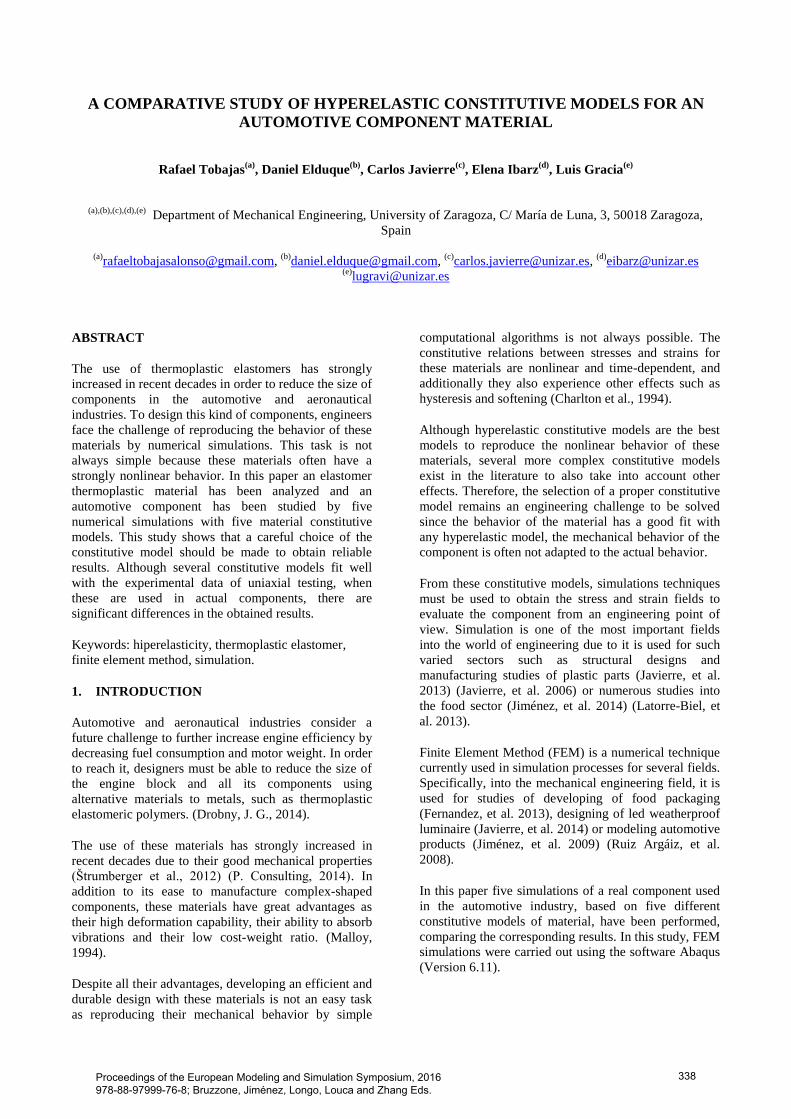
ABSTRACT

The use of thermoplastic elastomers has strongly

increased in recent decades in order to reduce the size of

components in the automotive and aeronautical

industries. To design this kind of components, engineers

face the challenge of reproducing the behavior of these

materials by numerical simulations. This task is not

always simple because these materials often have a

strongly nonlinear behavior. In this paper an elastomer

thermoplastic material has been analyzed and an

automotive component has been studied by five

numerical simulations with five material constitutive

models. This study shows that a careful choice of the

constitutive model should be made to obtain reliable

results. Although several constitutive models fit well

with the experimental data of uniaxial testing, when

these are used in actual components, there are

significant differences in the obtained results.

Keywords: hiperelasticity, thermoplastic elastomer,

finite element method, simulation.

1. INTRODUCTION

Automotive and aeronautical industries consider a

future challenge to further increase engine efficiency by

decreasing fuel consumption and motor weight. In order

to reach it, designers must be able to reduce the size of

the engine block and all its components using

alternative materials to metals, such as thermoplastic

elastomeric polymers. (Drobny, J. G., 2014).

The use of these materials has strongly increased in

recent decades due to their good mechanical properties

(Štrumberger et al., 2012) (P. Consulting, 2014). In

addition to its ease to manufacture complex-shaped

components, these materials have great advantages as

their high deformation capability, their ability to absorb

vibrations and their low cost-weight ratio. (Malloy,

1994).

Despite all their advantages, developing an efficient and

durable design with these materials is not an easy task

as reproducing their mechanical behavior by simple

computational algorithms is not always possible. The

constitutive relations between stresses and strains for

these materials are nonlinear and time-dependent, and

additionally they also experience other effects such as

hysteresis and softening (Charlton et al., 1994).

Although hyperelastic constitutive models are the best

models to reproduce the nonlinear behavior of these

materials, several more complex constitutive models

exist in the literature to also take into account other

effects. Therefore, the selection of a proper constitutive

model remains an engineering challenge to be solved

since the behavior of the material has a good fit with

any hyperelastic model, the mechanical behavior of the

component is often not adapted to the actual behavior.

From these constitutive models, simulations techniques

must be used to obtain the stress and strain fields to

evaluate the component from an engineering point of

view. Simulation is one of the most important fields

into the world of engineering due to it is used for such

varied sectors such as structural designs and

manufacturing studies of plastic parts (Javierre, et al.

2013) (Javierre, et al. 2006) or numerous studies into

the food sector (Jiménez, et al. 2014) (Latorre-Biel, et

al. 2013).

Finite Element Method (FEM) is a numerical technique

currently used in simulation processes for several fields.

Specifically, into the mechanical engineering field, it is

used for studies of developing of food packaging

(Fernandez, et al. 2013), designing of led weatherproof

luminaire (Javierre, et al. 2014) or modeling automotive

products (Jiménez, et al. 2009) (Ruiz Argáiz, et al.

2008).

In this paper five simulations of a real component used

in the automotive industry, based on five different

constitutive models of material, have been performed,

comparing the corresponding results. In this study, FEM

simulations were carried out using the software Abaqus

(Version 6.11).

Proceedings of the European Modeling and Simulation Symposium, 2016 978-88-97999-76-8; Bruzzone, Jiménez, Longo, Louca and Zhang Eds.

338

mailto:[email protected]




2. MATERIAL DESCRIPTION

An automotive air duct is going to be analyzed in this

paper. This component is made of a material called

Santoprene 101-73 provided by ExxonMobil

(ExxonMobil).

The nonlinear behavior of the material has been

described by uniaxial tensile tests like simple tension,

planar extension and simple compression. In addition,

cyclic behavior information is also provided at different

levels of deformation.

To characterize the material, the datasheet and Young

modulus value supplied by the manufacturer have been

used. This study focuses on the relationship between

stress and strain for the first pull deformation, when it is

the first time in deforming the material. The Young

modulus recommended by the manufacturer in this

deformation is E= 29.7 MPa (ExxonMobil). This

relationship can also be obtained from the cyclical

behavior information of the material, and it is

represented by a red line in Figures 1and 2. According

to standards (ASTM D412-15a) (ISO 37:2011), the

provided values of strain and stress are nominal values.

Figure 1: Strain-stress plot of Santoprene 101-73 from

manufacturer datasheet (ExxonMobil) for Simple

Tension.

Figure 2: Strain-stress plot of Santoprene 101-73 from

manufacturer datasheet (ExxonMobil) for Simple

Compression.

In order to obtain values of strain energy density, strain

and stress values from the first pull deformation shown

in Tables 1 and 2 are used. Strain energy density values

were obtained by Equation (1).

(1)

Strain, stress and strain energy density (SED) values

from the first pull deformation are shown in Tables 1

and 2.

Table 1: Strain-stress values for Santoprene 101-73

First Pull-Simple Tension

Nominal Strain

(%)

Nominal Stress

(MPa)

SED (MPa)

0.000 0.000 0.000

0.900 0.345 0.001

2.000 0.615 0.006

3.200 0.859 0.014

4.700 1.084 0.027

6.900 1.338 0.054

8.700 1.516 0.080

9.900 1.623 0.098

12.20 1.792 0.137

13.80 1.913 0.165

14.90 1.981 0.188

17.60 2.122 0.241

18.90 2.193 0.269

19.90 2.232 0.290

23.00 2.374 0.359

24.20 2.422 0.388

25.00 2.451 0.406

28.40 2.585 0.493

29.90 2.631 0.530

33.90 2.768 0.638

Table 2: Strain-stress values for Santoprene 101-73

First Pull-Simple Compression

Nominal Strain

(%)

Nominal Stress

(MPa)

SED (MPa)

0.00 0.000 0.0000

-0.90 -0.219 0.0010

-2.00 -0.437 0.0045

-3.20 -0.662 0.0114

-4.70 -0.884 0.0224

-6.90 -1.181 0.0454

-8.70 -1.399 0.0691

-9.90 -1.533 0.0866

-12.20 -1.783 0.1246

-13.80 -1.957 0.1543

-14.90 -2.086 0.1780

-17.60 -2.393 0.2380

-18.90 -2.550 0.2704

-19.90 -2.668 0.2955

-23.00 -3.066 0.3839

-24.20 -3.233 0.4224

-25.00 -3.338 0.4471

-28.40 -3.854 0.5715

-29.90 -4.088 0.6291


339

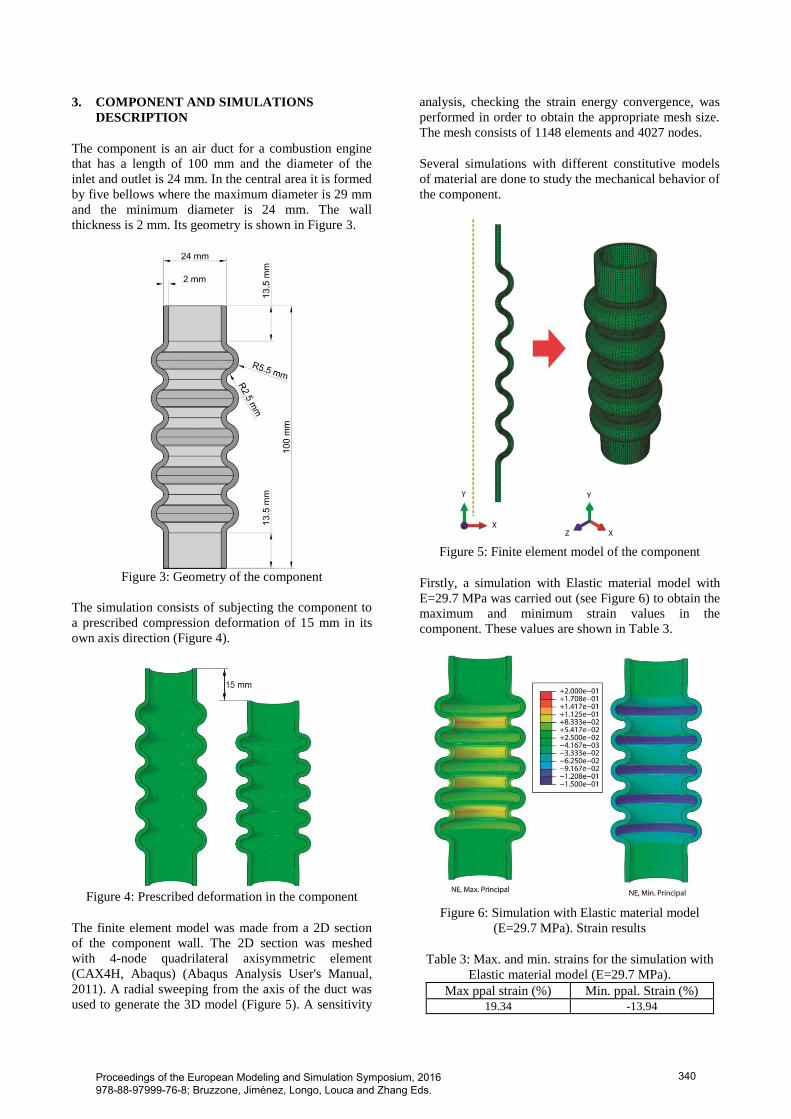
3. COMPONENT AND SIMULATIONS

DESCRIPTION

The component is an air duct for a combustion engine

that has a length of 100 mm and the diameter of the

inlet and outlet is 24 mm. In the central area it is formed

by five bellows where the maximum diameter is 29 mm

and the minimum diameter is 24 mm. The wall

thickness is 2 mm. Its geometry is shown in Figure 3.

Figure 3: Geometry of the component

The simulation consists of subjecting the component to

a prescribed compression deformation of 15 mm in its

own axis direction (Figure 4).

Figure 4: Prescribed deformation in the component

The finite element model was made from a 2D section

of the component wall. The 2D section was meshed

with 4-node quadrilateral axisymmetric element

(CAX4H, Abaqus) (Abaqus Analysis User's Manual,

2011). A radial sweeping from the axis of the duct was

used to generate the 3D model (Figure 5). A sensitivity

analysis, checking the strain energy convergence, was

performed in order to obtain the appropriate mesh size.

The mesh consists of 1148 elements and 4027 nodes.

Several simulations with different constitutive models

of material are done to study the mechanical behavior of

the component.

Figure 5: Finite element model of the component

Firstly, a simulation with Elastic material model with

E=29.7 MPa was carried out (see Figure 6) to obtain the

maximum and minimum strain values in the

component. These values are shown in Table 3.

Figure 6: Simulation with Elastic material model

(E=29.7 MPa). Strain results

Table 3: Max. and min. strains for the simulation with

Elastic material model (E=29.7 MPa).

Max ppal strain (%) Min. ppal. Strain (%)

19.34 -13.94


340

Then, the constants of hyperelastic models are going to

be fitted for each model and then the simulations with

these models are going to be carried out to compare the

results.

4. HYPERELASTICITY

The hyperelastic constitutive models are mathematical

models that attempt to simulate the behavior of

materials whose stress strain relationship is nonlinear.

Usually these models are represented by strain energy

density function W which is formulated as a function

depending on different magnitudes associated to the

strain field and the material constants, in the way:

(2)

where are principal stretches, and are

the invariants of left Cauchy-Green strain tensor, B,

respectively, obtained as:

(3)

(4)

(5)

In hyperelastic models the Cauchy stresses are derived

by differentiating the strain energy density function as

follows:

(6)

where F is the strain gradient tensor and et .

In this paper, five different constitutive models have

been used:

Linear elastic model

Hyperelastic Neo Hookean model

Hyperelastic Mooney-Rivlin model

Hyperelastic Ogden model

Hyperelastic Marlow model

4.1. Linear elastic model

In this model the material returns to its original shape

when the loads are removed, and the unloading path is

the same as the loading path. This model is known as

Hooke’s Law. The stress is proportional to the strain

and the constant of proportionality is the Young’s

modulus (E).

(7)

The strain energy density functions is defined as:

(8)

4.2. Hyperelastic Neo Hookean model

This model was proposed by Treloar in 1943 (Treloar, L

R.G., 1943). In this model, the strain energy density

function is based only on the first strain invariant:

(9)

where C1 is a material constant, J is the determinant of

the strain gradient tensor F and D is a material constant

related to the bulk modulus.

4.3. Hyperelastic Mooney-Rivlin model

The Mooney-Rivlin model (Mooney, 1940) (Rivlin, R.

S. and Saunders, D. W., 1951), proposed in 1951, is one

of the most used hyperelastic models in the literature.

Although there are various versions of this model, the

most general is based on the first and second strain

invariants. The strain energy density function is defined

as follows:

(10)

where Cij are material constants, J is the determinant of

the strain gradient tensor F and D is a material constant

related to the bulk modulus. Neo Hookean is a

particular case of the two parameters Mooney-Rivlin

model.

4.4. Hyperelastic Ogden model

The Ogden hyperelastic model (1972) (Ogden, R. W.,

1972) is possibly the most extended model after

Mooney-Rivlin model. This model is based on the three

principal stretches ( 1, 2, 3) and 2N material constants,

where N is the number of polynomials that constitute

the strain energy density function, defined as:

(11)

where μi y αi are material constants, J is the determinant

of the strain gradient tensor F and D is a material

constant related to the bulk modulus.

4.5. Hyperelastic Marlow model

The Marlow hyperelastic model (2003) (Marlow, R. S. ,

2003) means the strain energy density is independent of

the second invariant, and a single test such as a uniaxial


341

tension test is necessary to determine the material

response. The strain energy density function is defined

as:

(12)

where T(ε) is the nominal uniaxial stress and λT is the

uniaxial stretch.

4.6. Fitting parameters of material models

For all the previously presented models, the optimal

constant values were obtained by means of an

optimization algorithm to try to faithfully reproduce the

material behaviour provided by the manufacturer. A

least squares algorithm was used to minimize this

variable. The error function is defined as:

(13)

where m is the number of points on the chart provided

by the manufacturer.

Since the minimum principal strain provided on the

component is about -14% and the maximum principal

strain is 20%, the models have been adjusted to this

range of strain.

Once the optimal constant values were obtained, for

each model, the strain energy density and the strain-

stress curves were obtained and they were compared

with the actual material curves. To determine the

quality of each of the models, the R2 correlation

coefficient was calculated for the strain-stress plot

(Figure 7).

The values of material parameters and R2

values for the

models are shown in Table 4.

Table 4: Parameters and R2 values of models

Model Parameter Optimal

Value

R2

Linear elastic E 14.602 0.978

Hyperelastic

Neo Hookean C1 2.416 0.977

Hyperelastic

Mooney

Rivlin

C10 3.190

0.975 C01 -0.818

Hyperelastic

Ogden N=2

μ1 25.560

0.977 α1 0.065

μ2 76.579

α2 0.108

In view of the obtained results, all presented models fit

well with actual values of the material datasheet

because the R2 correlation coefficient is always higher

than 0.960. Therefore any of the studied models should

provide good results in the simulation of the

component.

Figure 7: Strain-stress plot for different models

between -14% and 20% strain

5. SIMULATIONS AND RESULTS

In order to check the mechanical behavior of the

component depending on the constitutive model used,

five finite element simulations of the duct compression

were performed. Each of them uses one of the different

material constitutive models introduced in Section 3.

Figure 8: Four characteristic elements of the model

The values of the variables most commonly used in the

engineering field, like stresses, strains and energy, have

been obtained from integration points of four

characteristic elements of the model (Figure 8).


342

In several studies maximum principal strain and the

strain energy density were used to evaluate the life of

component when a cyclic load was applied to it. (Mars,

W. V., & Fatemi, A., 2002). Other investigations about

fatigue use maximum principal stresses to calculate the

life of component. (André, N., Cailletaud, G., & Piques,

R., 1999). Finally, the Von Mises comparison stress is

commonly used to know if the material is able to resist

a static load or displacement.

So, concerning the strain field, the maximum and the

minimum principal strains, respectively, were studied

(Figures 9 and 10). On the other hand, for the stress

field, the maximum and minimum principal stresses,

respectively, (Figures 11 and 12) and the von Mises

stress were analyzed (Figure 13) at each of the

integration points and these values were referred at

centroid of elements. And finally, the strain energy

density was also studied (Figure 14).

6. DISCUSSION

The obtained results show that the mechanical behavior

of Santoprene 101-73 can be accurately adjusted by

using the different models of hyperelastic behavior

considered with the appropriate material constants, with

a good agreement with the data supplied by the

manufacturer for the uniaxial stress-strain curve. A least

squares algorithm allows obtaining the material

constant reaching values of R2 over 0.975 in all studied

models when applied for stress-strain uniaxial curve.

However, important differences were found in stresses

(up to 40%) and the strain energy density (up to 90%)

when the models were applied to a real component in a

wide range of strain as occurs in the normal operation of

that kind of pieces.

To this respect, the pure elastic, the NeoHookean, the

Mooney-Rivlin and the Ogden models provide similar

results as much in principal strains as in principal

stresses. A similar trend is observed for von Mises

stress and strain energy density.

A more realistic behavior is obtained by using Marlow

model and important divergences were found respect

the other models. The divergence is more pronounced

for stresses and strain energy density, whereas it is

considerably lesser for strains.

So, a careful election of the appropriate constitutive

model must be done in order to obtain realistic

simulations of real components, in such a way that the

results corresponding to strains and stresses would be

reliable enough, allowing the strength and functionality

verifications, considering that those magnitudes are

used to predict mechanical performance, fatigue life,

etc., and then can determine important features of the

component design.

7. CONCLUSIONS

The aim of this paper was to determine the best

constitutive model for reproducing the mechanical

behavior of Santoprene 101-73, material used in

automotive industry. To reach it, four different

hyperelastic models and the commonly used linear

elastic model have been studied in order to obtain the

material constants of each of them. An optimization

least squares algorithm were used to fit the best values

of material constants to each of them. In order to

conclude which of them best represents the actual

behavior of the material, the R2 correlation coefficient

for stress-strain relationship has been used.

In view of the obtained results, it can be concluded that

all the considered models fit the actual material

behavior with enough accuracy, being the Marlow

model the most accurate model to reproduce the

mechanical behavior of Santoprene 101-73, considering

the stress-strain uniaxial curve.

However, the study has demonstrated that despite using

constitutive models that fit correctly to the actual

behavior of the material in standardized uniaxial tests,

the different models show large differences concerning

the realistic behavior when they are applied to real

components, in which complex stress/strain fields can

arise. So, more information from biaxial and planar tests

is needed in order to perform accurate simulations for

real components.


343

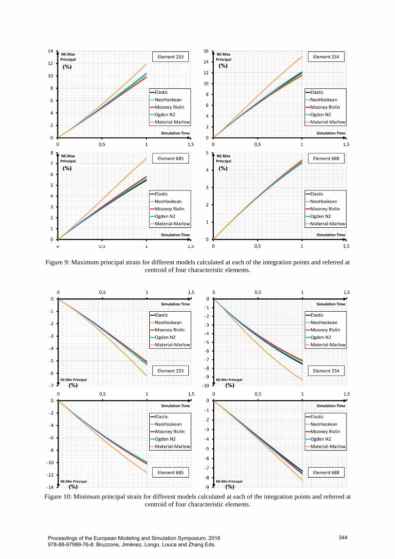
Figure 9: Maximum principal strain for different models calculated at each of the integration points and referred at

centroid of four characteristic elements.

Figure 10: Minimum principal strain for different models calculated at each of the integration points and referred at



344

Figure 11: Maximum principal stress for different models calculated at each of the integration points and referred at


Figure 12: Minimum principal stress for different models calculated at each of the integration points and referred at



345

Figure 13: Von Mises comparison stress for different models calculated at each of the integration points and referred at


Figure 14: Strain energy density (SED) for different models calculated at each of the integration points and referred at



346

REFERENCES

Abaqus Analysis User's Manual, Abaqus 6.11 Online

Documentation, Dassault Systèmes, 2011.

André, N., Cailletaud, G., & Piques, R. (1999). Haigh

diagram for fatigue crack initiation prediction of

natural rubber components. Kautschuk Gummi

Kunststoffe, 52(2), 120-123.

ASTM D412-15a, Standard Test Methods for

Vulcanized Rubber and Thermoplastic

Elastomers—Tension, ASTM International, West

Conshohocken, PA, 2015, www.astm.org

Charlton, D. J., Yang, J., The, K K., A Review of

Methods to Characterize Rubber Elastic Behavior

for Use in Finite Element Analysis, Rubber

Chemistry and Technology (3) 481–503.1994

Drobny, J. G. (2014). Handbook of thermoplastic

elastomers. Elsevier.

Dufton, P. W. (2001). Thermoplastic Elastomers

Market. iSmithers Rapra Publishing.

ExxonMobil, Santoprene 101-73 Thermoplastic

Vulcanizate.

Fernández, A., Javierre, C., González, J. & Elduque, D.,

2013. Development of thermoplastic material food

packaging considering technical, economic and

environmental criteria. Journal of Biobased

Materials and Bioenergy, 7(2), 176-183.

ISO 37:2011. Rubber, vulcanized or thermoplastic –

determination of tensile stress–strain properties.

ISO Standard; 2011.

Javierre, C., Abad-Blasco, J., Camañes & V., F. D.,

2013. Redesign of metalic parts with thermoplastic

materials: Application example | Rediseño de

componentes metálicos En materiales

termoplásticos: Ejemplo de aplicación. DYNA,

88(2), 197-205.

Javierre, C., Elduque, D., Camañes, V. & Franch, D.

(2014). Simulation and experimental analysis of

led weather proof luminaire thermal performance.

Paper presented at the 26th European Modeling

and Simulation Symposium, EMSS 2014.

Javierre, C., Fernández, A., Aísa, J. & Clavería, I.,

2006. Criteria on feeding system design:

Conventional and sequential injection moulding.

Journal of Materials Processing Technology,

171(3), 373-384.

Jiménez, E. et al. 2014. Methodological approach

towards sustainability by integration of

environmental impact in production system

models through life cycle analysis: Application to

the Rioja wine sector. SIMULATION, 90(2),

pp.143-161.

Jiménez, E., Ruiz, I., Blanco, J., & Pérez, M. (2009).

Design and simulation of production of injection

pieces in automobile industry. International

Journal of Simulation: Systems, Science and

Technology, 10(3), 23-30.

Kutz, M. (Ed.). (2011). Applied plastics engineering

handbook: processing and materials. William

Andrew.

Latorre-Biel, J. I., Jiménez-Macías, E., Blanco-

Fernández, J., & Sáenz-Díez, J. C. (2013b).

Optimal design, based on simulation, of an olive

oil mill. Paper presented at the 25th European

Modeling and Simulation Symposium, EMSS 2013.

Mars, W. V., & Fatemi, A. (2002). A literature survey

on fatigue analysis approaches for rubber.

International Journal of Fatigue, 24(9), 949-961.

Marlow, R. S. (2003). A general first-invariant

hyperelastic constitutive model. Constitutive

Models for Rubber, 157-160.

Mooney, M. (1940). A theory of large elastic

deformation. Journal of applied physics, 11(9),

582-592.

Ogden, R. W. (1972, February). Large deformation

isotropic elasticity-on the correlation of theory and

experiment for incompressible rubberlike solids.

In Proceedings of the Royal Society of London A:

Mathematical, Physical and Engineering Sciences

(Vol. 326, No. 1567, pp. 565-584). The Royal

Society.

P. Consulting, Global elastomeric polyolefins markets,

technologies trends (2014) 2014–2020.

Rivlin, R. S., & Saunders, D. W. (1951). Large elastic

deformations of isotropic materials. VII.

Experiments on the deformation of rubber.

Philosophical Transactions of the Royal Society of

London A: Mathematical, Physical and

Engineering Sciences, 243(865), 251-288.

Robert A.. Malloy. (1994). Plastic part design for

injection molding: an introduction. Hanser

Publishers.

Ruiz Argáiz, I., Jiménez Macías, E., Blanco Fernández,

J., & Pérez de la Parte, M. (2008). Design and

simulation of production of injection pieces in

automobile industry. Paper presented at the

Proceedings -EMS 2008, European Modelling

Symposium, 2nd UKSim European Symposium on

Computer Modelling and Simulation.

Štrumberger, N., Gospočić, A., & Bartulić, Č. (2012).

Polymeric Materials in Automobiles. PROMET-

Traffic&Transportation, 17(3), 149-160.

Treloar, L. R. G. (1943). The elasticity of a network of

long-chain molecules—II. Transactions of the

Faraday Society, 39, 241-246.


347

http://www.astm.org/

a comparative study of hyperelastic ... - home - msc-les

Documents