a comparative study of multiple regression analysis and

A Comparative Study of Multiple Regression Analysis and Back

Propagation Neural Network Approaches for Predicting Financial

Strength of Banks: An Indian Perspective YAZED ALSAAWY1, AHMAD ALKHODRE2, MOHAMMED BENAIDA3

RAFI AHMAD KHAN4 1,2,3Department of Information Technology, Faculty of Computer Science and Information System

Islamic University of Madinah, Medina, SAUDI ARABIA 4Department of Management Studies, University of Kashmir, INDIA

Abstract: - The main motivation of this study is to forecast the performance of Indian banks using multiple regression analysis and artificial neural network and to compare these two methods for the accuracy. To achieve this goal, financial data spread over 10 years from 2010 to 2019 was collected from 19 Indian public sector banks. The data consists of 17 financial ratios collected from financial statements and other publications of the sample organizations. Capital Adequacy Ratio (CRAR) has been chosen as dependent variable for measuring and predicting the financial strength of banks. Identification of significant ratios that are determinants of CRAR are identified by using regression technique then these identified ratios are used as input for a developing a neural network model. The findings of multi-linear regression analysis identified 7 financial ratios that have a positive relationship between with dependent variable (CRAR). These 7 dependent variables were used to predict the financial strength (CRAR) of the Banks. Then a feed forward back propagation neural network was developed with these 7 dependent variables to predict the CRAR. Finally, the performances of these two methods were measured by using the Mean Square Error (MSE), Root Mean Squared Error (RMSE) and Mean Absolute Percent Error (MAPE). The results indicate that ANN model scores an improvement of 55.67% in MSE over regression model. In RMSE which re-scales the errors in order to keep the errors’ dimension as the predicted value, ANN model scores an improvement of 33.425% over regression model. It also indicates that ANN model scores an improvement of 99.32% over regression model in MAPE which measures the magnitude of absolute errors in relative terms. Results show that ANN model outperforms the regression model and is superior technique of forecasting CRAR of Indian Banks.

Key-Words: - Machine Learning (ML), Regression, Artificial Neural Networks (ANN), Capital Adequacy Ratio (CRAR), Financial Ratios, Financial Strength, Bankruptcy

Received: April 18, 2019. Revised: May 30, 2020. Accepted: June 8, 2020. Published: June 10, 2020 1 Introduction Financial Institutions play a vital role in the economy and several studies contend that the efficiency of financial intermediation affects economic growth. Thus, the financial strength of banks has been an issue of main interest for various stakeholders such as regulators, depositors, investors, and customers. Traditionally, the financial strength of banks has been assessed on the basis of financial ratios but the advances in statistical techniques and machine learning techniques have resulted in a move towards the use of such techniques. After examining the related literature, it was revealed that multi-linear regression technique is the

most commonly used statistical technique to predict the financial strength of the financial institutions. Regression technique is simple for figuring out the financial strength of the financial institutions and therefore widely used to measure the performance of these institutions. When there is no suitable mathematical relationship between independent and dependent variables, then machine learning technique of neural network can be used to get better results. Therefore, this study uses both regression and artificial neural networks (ANN) to develop models for predicting the financial stability of the financial institutions. This study has made comparison of prediction accuracy of these methods

WSEAS TRANSACTIONS on BUSINESS and ECONOMICS DOI: 10.37394/23207.2020.17.60

Yazed Alsaawy, Ahmad Alkhodre, Mohammed Benaida, Rafi Ahmad Khan

E-ISSN: 2224-2899 627 Volume 17, 2020

find out the a most appropriate tool for prediction of financial strength of financial institutions. 2 Literature Review Various studies have identified the factors responsible for the financial strength and profitability of the bank and have used these factors for measuring and predicting the performance of the banks. In a review of empirical measurements of bank performance, two broad methods: nonstructural and structural were distinguished by [1]. A non-structural approach is based on selection of financial ratios that can measure the various features of performance, whereas a structural approach usually depends on on the economics of profit maximization or cost minimization. Since, this study is focused on modeling the data which is in the form of bank ratios to predict the profitability of banks, therefore, it shuns a structural approach in favor of a nonstructural one. Review of literature reveals that most of the research on finding the profitability of bank are focused on developed countries and there are only a few of studies based on developing countries [3]; [4]; [5] but most of these studies have used mostly the same variables. Several researches have used CAMEL (Capital adequacy, Asset quality, Management efficiency, Earnings performance and Liquidity) to study factors that affect the profitability of the banks [8]; [9]. CAMEL was developed by the US Federal Deposit Insurance Corporation (FDIC) for early identification of problems in banks operations. Although there are various other bank assessment models but CAMEL model has emerged as most commonly used which is even recommended by various international organizations like IMF [10]. In this study, CAMEL rating system has been chosen as a basis because it allows gauging the bank’s overall condition and performance. However, it should be noted that this system is not standardized and is very comprehensive. Due to this, it is hard if not impossible to assess the performance of the banks covered in this study. In this regard, this study has selected ratios which could serve as a substitution to certain elements of CAMEL system. Capital Adequacy is one the important determinant of banks performance as evidenced by the literature. The issue of capital adequacy requirement originates from the work of Brechling & Clayton (1965) who raised the issue of probable existence of optimum level of owners’ equity which banks would prefer to maintain in order to ensure the stability of banks with the simultaneous effective

use of available own financial resources [11]. In an empirical study conducted by Pelzman in 1970’s concluded that both the level of bank capital and its distribution would be about the same if the regulatory apparatus had never come into being [12]. Christian et al. demonstrated that capital adequacy among other variables is the most informative source for assessing banks’ returns [13]. Minimum capital requirements are being considered as the primary means of stabilizing banking sector by a growing literature. According to Basel Accord, the regulators around the world agree that capital adequacy is vital but it has been observed that nations tend to weaken this agreement by applying capital rules and regulations discriminately [14]. In the last few decades, Machine learning method of ANN has emerged as the widely used technique for bankruptcy prediction, fraud detection of credit cards and insurance, loan evaluation [15]. The performance comparison of ANN has been carried out with various traditional statistical methods like with multiple linear regression [17] and [18], discriminant analysis and logistic regression [19], decision trees and logistic regression [20], stepwise regression and ridge regression [21], logistic regression [22]. In almost all of these studies, has outclassed these traditional techniques. In fact, it has been established that performance of ANN is far better than multiple regression especially when the size of date is large[17]. Nowadays, ANNs are widely used to predict the bankruptcy of companies especially banks [23] [24]. Boritz & Kennedy (1995) studied various types of ANN and then compared their performance with various other traditional bankruptcy prediction methods such as discriminant analysis, logit and probit techniques [25]. In fact, results of numerous other studies that have made such comparison reveal that prediction accuracy of ANN exceeds all other methods [26]; [27]; [28]; [29]; [30]; [31]; [32]; [33]; [34]; [35]; [36]; [37]. Only advantage that these traditional methods have is that they are easy to understand and use [38]. With the above literature signifying the neural network technique in prediction of the performance of banks, this study has used both techniques in conjunction. CRAR has been chosen as dependent variable for measuring and predicting the financial strength of banks. Identification of significant ratios that are determinants of CRAR are identified by using regression techniques then these identified ratios are used as input for a developing a neural network model. In the next sections, an attempt has been made to develop a CRAR prediction model



E-ISSN: 2224-2899 628 Volume 17, 2020

from the data. The model thus developed has been tested on the real data obtained from the sample organizations. 3 Selection of Variables The data for the study was collected from 19 public sector banks from Indian banking industry. The financial data was collected from financial statements and other publications of the sample organizations. The data thus collected were analyzed through 17 financial ratios labeled from V1 to V17 as presented in table 1. The financial data spread over 10 years from 2010 to 2019 about these ratios were collected from sample organizations and analyzed through various financial tools. 4 Model Development through

Regression In order to build the model, CRAR (V1) has been taken as dependent variable, keeping in view the nature of this variable and expert opinion. Thus, Multiple Regression was run with CRAR (V1) as dependent variable and all other variables from V2 to V17 were included as independent variables to build the model. The regression was run in MS-Excel by XLSTAT with stepwise method. Stepwise regression technique attempts to find out

the significant variables of a model by adding or subtracting them and consequently creates a model that is more accurate in predictions. Forward stepwise regression adds the variables on the basis

of their ability to positively influence the prediction competency of the model which is primarily based on the level of significance or p-value. When a variable is added, the model is re-evaluated to find out if any other variable can be added. Once there are no more variables that can be added to the model, the stepwise regression stops and the model is used as final. This final model is then used for predicting the outcome of dependent variables i.e., output based on independent variables i.e., inputs [39].

Table 2, depicts the different steps of stepwise selection of variables. The stepwise regression in our study extracted only seven variables V2, V5, V7, V8, V9, V14 and V16 that have significant effect on dependent variable CRAR(V1) out of total sixteen independent variables as significant. This model has R2 value of 0.531 and has the lowest MSE at 1.185 among all the models tested by stepwise regression, hence these seven variables have been included in the final model. Hence the regression model is represented as

1 2 5 7 8 90 1 2 2 2 214 162 2

V V V V V V

V V

Table 1: Ratios

Ratio Name Var Type Var

Name Capital Adequacy Ratio Dependent V1 Return on Net Worth (%) Independent V2 Interest Income / Total Funds Independent V3 Net Interest Income / Total Funds Independent V4 Non-Interest Income / Total Funds Independent V5 Interest Expended / Total Funds Independent V6 Net Profit / Total Funds Independent V7 Advances / Loans Funds (%) Independent V8 Financial Charges Coverage Ratio Independent V9 Interest Spread Independent V10 Net Profit Margin Independent V11 Return on Long Term Fund (%) Independent V12 Operating Expense / Total Funds Independent V13 Net NPA To Net Advances Independent V14 Credit - Deposit Ratio Independent V15 Return on Advances Adjusted to Cost of Funds

Independent V16 Return on Investments Adjusted to Cost of Funds

Independent V17

Table 2: Regression Results

No of

Var Variables

Variable

IN/OUT Status MSE R²

Adjusted

R²

1 V11 V11 IN 1.682 0.307 0.303 2 V2/V11 V2 IN 1.546 0.367 0.359 3 V2/V7/ V11 V7 IN 1.492 0.393 0.381

4 V2/V7/V11/ V14

V14 IN 1.393 0.437 0.423

3 V2/ V7/ V14 V11 OUT 1.384 0.437 0.426

4 V2/ V7/ V8 / V14

V8 IN 1.296 0.476 0.463

5 V2/V5/V7/ V8/V14

V5 IN 1.242 0.501 0.485

6 V2/V5/V7/ V8/V9/V14

V9 IN 1.214 0.516 0.497

7 V2/V5/V7/ V8/V9/V14 /V16

V16 IN 1.185 0.531 0.509



E-ISSN: 2224-2899 629 Volume 17, 2020

Table 3: Goodness of Fit Statistics

Observations 160

Sum of weights 160

DF 152

R² 0.531

Adjusted R² 0.509

MSE 1.185

RMSE 1.088

MAPE 6.433

DW 1.323

Observations: The number of observations used is 160.

DF: Degrees of freedom or the number for the selected model is 152

R²: The R² which determines the proportion of the variance in dependent variables is 0.531.

Adjusted R²: The adjusted determination coefficient R² which is improvement to the R² takes into consideration the number of variables used in the model is 0.509.

MSE: The mean of the squares of the errors (MSE) value is equal to 1.185

n

ForecastActualMSE

∑ 2)(

RMSE: It is the square root of the MSE and is

equal to 1.088.

n

predictedvactualvRMSE

∑ 2)(1-)(1(

MAPE: The Mean Absolute Percentage Error

(MAPE) is 6.433.

n

Xactualv

predictedvactualv

MAPE

100)(1

∑ )(1)(1

DW: The Durbin-Watson statistic is calculated

by the formula

∑1

2

∑1

2)1(

n

tte

n

ttete

d

Where e1, e2… etc, are the time-ordered errors. The value of Durbin-Watson always lies between 0 and 4. If the value falls close to 0 then it indicates the positive autocorrelation, while as the value that is close to 4 indicates that there is negative autocorrelation. As shown in table 3, DW is equal to 1.323 which shows there is no first-order autocorrelation, either positive or negative.

5 Model Development through Neural

Network

With the ever-increasing recognition and dependence of the financial world on modern technology, several neural network models have been proposed and tested in various fields of finance over last few years. Majority of these NN models are based on backpropagation with one hidden layer which have outperformed traditional statistical models [40].

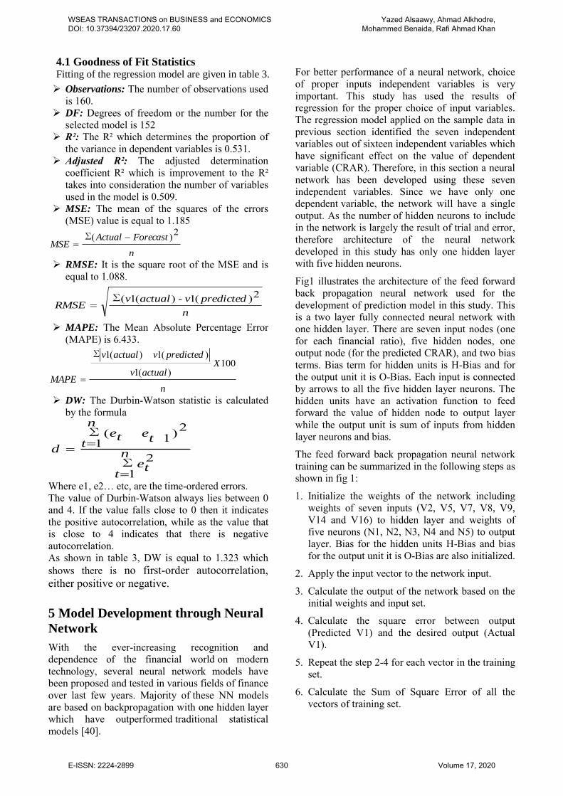
For better performance of a neural network, choice of proper inputs independent variables is very important. This study has used the results of regression for the proper choice of input variables. The regression model applied on the sample data in previous section identified the seven independent variables out of sixteen independent variables which have significant effect on the value of dependent variable (CRAR). Therefore, in this section a neural network has been developed using these seven independent variables. Since we have only one dependent variable, the network will have a single output. As the number of hidden neurons to include in the network is largely the result of trial and error, therefore architecture of the neural network developed in this study has only one hidden layer with five hidden neurons.

Fig1 illustrates the architecture of the feed forward back propagation neural network used for the development of prediction model in this study. This is a two layer fully connected neural network with one hidden layer. There are seven input nodes (one for each financial ratio), five hidden nodes, one output node (for the predicted CRAR), and two bias terms. Bias term for hidden units is H-Bias and for the output unit it is O-Bias. Each input is connected by arrows to all the five hidden layer neurons. The hidden units have an activation function to feed forward the value of hidden node to output layer while the output unit is sum of inputs from hidden layer neurons and bias.

The feed forward back propagation neural network training can be summarized in the following steps as shown in fig 1:

1. Initialize the weights of the network including weights of seven inputs (V2, V5, V7, V8, V9, V14 and V16) to hidden layer and weights of five neurons (N1, N2, N3, N4 and N5) to output layer. Bias for the hidden units H-Bias and bias for the output unit it is O-Bias are also initialized.

2. Apply the input vector to the network input.

3. Calculate the output of the network based on the initial weights and input set.

4. Calculate the square error between output (Predicted V1) and the desired output (Actual V1).

5. Repeat the step 2-4 for each vector in the training set.

6. Calculate the Sum of Square Error of all the vectors of training set.



E-ISSN: 2224-2899 630 Volume 17, 2020

4.1 Goodness of Fit Statistics Fitting of the regression model are given in table 3.

7. Propagate error backward and adjust the weights and bias terms of input to hidden layer and hidden layer to output layer in such a way that minimizes Sum of Square Error.

8. Repeat steps 3-7 until the error for the set is lower than the required minimum error.

Neural network is trained by reiterations of these steps which result in reduction of the error between the actual outputs and target outputs to an acceptable value. Then the developed neural network model is tested and validated on test data to check the accuracy and robustness of the.

5.1 Feed Forward Back propagation ANN

(With Exponential Activation Function)

The data consisted of seven ratios that were found to be significant determinants of dependable variable i.e., CRAR (V1) through stepwise regression in the previous chapter. Since the sample organizations considered for this study are nineteen and the spread of data is ten years, therefore, total observation are 190. Out of these 190 observations, 160

observations have been used as training data set and rest 30 observations as testing data set. The training data set consisting of 160 observations is presented in columns A through J of the spreadsheet as shown in fig 2. Since the objective of this study is to develop a NN model that can predict the CRAR of the sample banks for next year on the basis of value of independent variables of the current year. Therefore, in order to train the NN perfectly, the value of actual CRAR (V1) of every observation is one year ahead.

O-Bias

V9

V8

V5

V7

VI6

V2

VI4

Predicted

VI

N4

N5

N3

N2

NI

H-Bias

Actual

VI

Square of Difference

Hidden Neuron

Weights

Hidden Input

Weights

Minimize Difference by

Adjusting Weights

Fig 1. Back Propagation Neural Network

Input Layer Hidden Neuron Layer

Output Layer



E-ISSN: 2224-2899 631 Volume 17, 2020

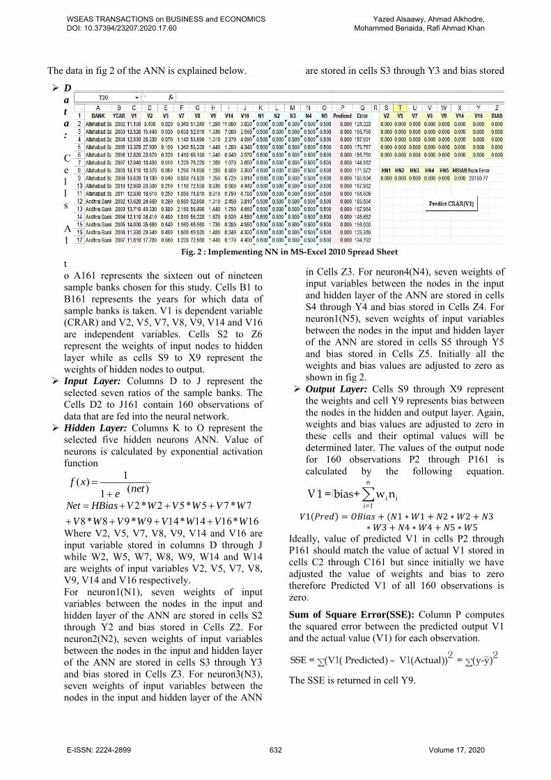
The data in fig 2 of the ANN is explained below.

D

a

t

a

:

Cells A1 to A161 represents the sixteen out of nineteen sample banks chosen for this study. Cells B1 to B161 represents the years for which data of sample banks is taken. V1 is dependent variable (CRAR) and V2, V5, V7, V8, V9, V14 and V16 are independent variables. Cells S2 to Z6 represent the weights of input nodes to hidden layer while as cells S9 to X9 represent the weights of hidden nodes to output.

Input Layer: Columns D to J represent the selected seven ratios of the sample banks. The Cells D2 to J161 contain 160 observations of data that are fed into the neural network.

Hidden Layer: Columns K to O represent the selected five hidden neurons ANN. Value of neurons is calculated by exponential activation function

)(1

1)(net

exf

16*1614*149*98*87*75*52*2

WVWVWVWV

WVWVWVHBiasNet

Where V2, V5, V7, V8, V9, V14 and V16 are input variable stored in columns D through J while W2, W5, W7, W8, W9, W14 and W14 are weights of input variables V2, V5, V7, V8, V9, V14 and V16 respectively. For neuron1(N1), seven weights of input variables between the nodes in the input and hidden layer of the ANN are stored in cells S2 through Y2 and bias stored in Cells Z2. For neuron2(N2), seven weights of input variables between the nodes in the input and hidden layer of the ANN are stored in cells S3 through Y3 and bias stored in Cells Z3. For neuron3(N3), seven weights of input variables between the nodes in the input and hidden layer of the ANN

are stored in cells S3 through Y3 and bias stored

in Cells Z3. For neuron4(N4), seven weights of input variables between the nodes in the input and hidden layer of the ANN are stored in cells S4 through Y4 and bias stored in Cells Z4. For neuron1(N5), seven weights of input variables between the nodes in the input and hidden layer of the ANN are stored in cells S5 through Y5 and bias stored in Cells Z5. Initially all the weights and bias values are adjusted to zero as shown in fig 2.

Output Layer: Cells S9 through X9 represent the weights and cell Y9 represents bias between the nodes in the hidden and output layer. Again, weights and bias values are adjusted to zero in these cells and their optimal values will be determined later. The values of the output node for 160 observations P2 through P161 is calculated by the following equation.

n

i ii=1

V1= bias+ w n∑

𝑉1(𝑃𝑟𝑒𝑑) = 𝑂𝐵𝑖𝑎𝑠 + (𝑁1 ∗ 𝑊1 + 𝑁2 ∗ 𝑊2 + 𝑁3∗ 𝑊3 + 𝑁4 ∗ 𝑊4 + 𝑁5 ∗ 𝑊5

Ideally, value of predicted V1 in cells P2 through P161 should match the value of actual V1 stored in cells C2 through C161 but since initially we have adjusted the value of weights and bias to zero therefore Predicted V1 of all 160 observations is zero.

Sum of Square Error(SSE): Column P computes the squared error between the predicted output V1 and the actual value (V1) for each observation.

SSE = (V ( Predicted) – V (Actual)) = (y-y)2 2

1 1∑ ∑

The SSE is returned in cell Y9.

Fig. 2 : Implementing NN in MS-Excel 2010 Spread Sheet



E-ISSN: 2224-2899 632 Volume 17, 2020

After the basic ANN model is put in place, the next step is to run each of the observations through the ANN. It is important to note that as in regression, it is necessary to determine the weights for the ANN that minimize the sum of squared errors to the least. Cognizance has also been taken of that the values of weights and biases are dynamic i.e., if there is change in the values of the weights and the value of computed hidden nodes then output i.e., V1 (Predicted) will be automatically updated. The back-propagation NN typically computes the optimal weights for an ANN which is implemented in this study through Solver.

5.2 Training the Neural Network

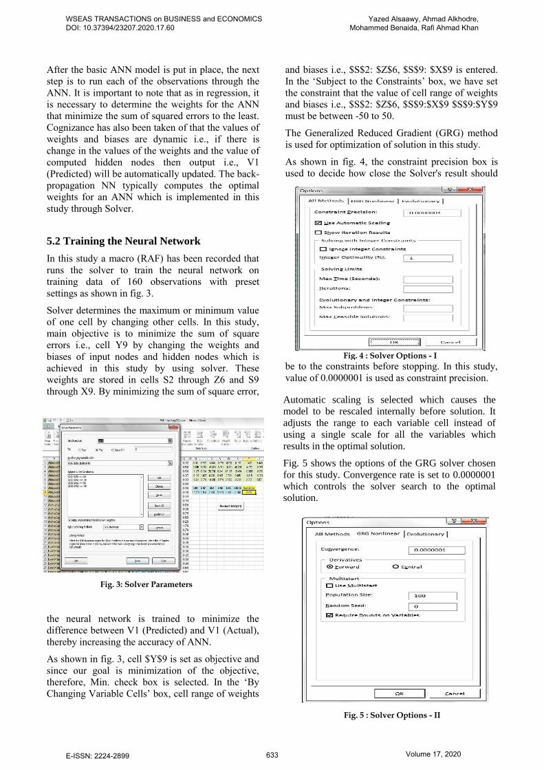
In this study a macro (RAF) has been recorded that runs the solver to train the neural network on training data of 160 observations with preset settings as shown in fig. 3.

Solver determines the maximum or minimum value of one cell by changing other cells. In this study, main objective is to minimize the sum of square errors i.e., cell Y9 by changing the weights and biases of input nodes and hidden nodes which is achieved in this study by using solver. These weights are stored in cells S2 through Z6 and S9 through X9. By minimizing the sum of square error,

the neural network is trained to minimize the difference between V1 (Predicted) and V1 (Actual), thereby increasing the accuracy of ANN.

As shown in fig. 3, cell $Y$9 is set as objective and since our goal is minimization of the objective, therefore, Min. check box is selected. In the ‘By Changing Variable Cells’ box, cell range of weights

and biases i.e., $S$2: $Z$6, $S$9: $X$9 is entered. In the ‘Subject to the Constraints’ box, we have set the constraint that the value of cell range of weights and biases i.e., $S$2: $Z$6, $S$9:$X$9 $S$9:$Y$9 must be between -50 to 50. The Generalized Reduced Gradient (GRG) method is used for optimization of solution in this study.

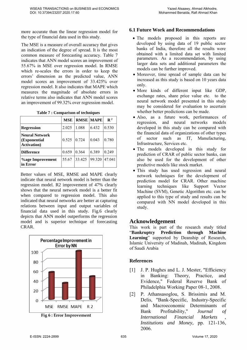
As shown in fig. 4, the constraint precision box is used to decide how close the Solver's result should

be to the constraints before stopping. In this study, value of 0.0000001 is used as constraint precision.

Fig. 4 : Solver Options - I

Fig. 5 : Solver Options - II

Fig. 3: Solver Parameters



E-ISSN: 2224-2899 633 Volume 17, 2020

Automatic scaling is selected which causes the

model to be rescaled internally before solution. It

adjusts the range to each variable cell instead of

using a single scale for all the variables which

results in the optimal solution.

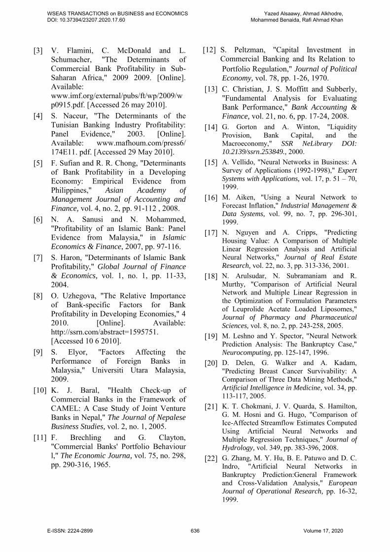
Fig. 5 shows the options of the GRG solver chosen

for this study. Convergence rate is set to 0.0000001

which controls the solver search to the optimal

solution.

Require Bounds on Variables option is selected as it speeds up the process of finding the solution by limiting the array of values to lower and upper bounds that the Solver must explore.

The forward derivative tries to discover the optimal solution. It guesses the first derivative at a point by disturbing the point once in a forward direction and computing the rise over the run. Central approximations are obtained by disturbing far from the point in both backward and forward directions to compute the rise over the run. Central differences deliver a further precise guess of the derivative, but it takes double number of computations that means it twice slower. 5.3 Training Results

Both options were tried in this study and the results are depicted in table 4. Initially the Sum of Square Error was 25912.95. Which was reduced to 103.9 after solver was run three times using forward derivative approach. There was marginal reduction in error after the second run. However, central derivative approach provided better results by reducing the error to 84.02 in second run only. There was no reduction in error in the subsequent runs. Therefore, central derivative approach is selected in this study.

5.4 Testing the Neural Network

The trained network was then tested on the testing data of 30 observation of the sample banks to check the robustness and accuracy of the developed NN model.

of the developed model.

Comparison of training and testing results is presented in table 6. R2 value of testing data was 0.731 which vary by 6.4% only but within the accuracy limit of ±10%. MAPE shows and improvement of 42.8% over training data. This testing result indicate the reliability and robustness

6 Conclusion

CRAR was selected as dependent variable as literature signified the relevance of this ratio for measuring the performance of banks. The financial data used for development of models consisted of seventeen financial ratios of nineteen public sector banks and spread over ten years was collected from Indian banking industry. Out of seventeen ratios, seven significant ratios were identified as determinants of CRAR by stepwise regression technique. These seven ratios were used as input for developing neural network model.

The regression model was used to supplement the ANN models by using its results for the proper choice of input independent variables. A comparison of the forecasting accuracy of regression model with the chosen ANN model is presented in table 7. It provides some insight into their performance and efficiency. Four common criteria of error measurement were used to compare the two models: Mean Square Error (MSE), the Root Mean Squared Error (RMSE), the Mean Absolute Percent Error (MAPE) and the R2. The table clearly suggests that the neural network is

Table 6 : Testing & Training Comparison

MAPE R Square

NN(Training) 0.044 0.780

NN(Testing) 0.028 0.731



E-ISSN: 2224-2899 634 Volume 17, 2020

Table 4 presents generated weight matrix of hidden

layer of the developed neural network model. The

W2, W5, W7, W8, W9, W14, W16 represent

weights of input nodes to five hidden neurons and

BIAS represents the bias values to five hidden

neurons.

Table 4: Training Results

Derivative

Method

No of

Runs

No of

Epochs

Sum of Square

Error

Forward

1 269 119.86

2 1402 104.02

3 56 103.9

Central

1 489 90.84

2 270 84.02

3 5 84.02

Table 5 represents the fitness of good statistics of

the developed model using central derivative

approach. R2 value of 0.78 is significant and

indicates that there is a strong correlation between

independent variables and dependent variable

(CRAR).

Table 5 : Error Measurement

MSE RMSE MAPE R Square

0.5251 0.7246 0.0437 0.7802

more accurate than the linear regression model for the type of financial data used in this study.

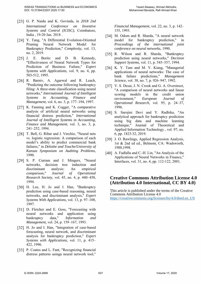
The MSE is a measure of overall accuracy that gives an indication of the degree of spread. It is the most common measure of forecasting accuracy. Table 7 indicates that ANN model scores an improvement of 55.67% in MSE over regression model. In RMSE which re-scales the errors in order to keep the errors’ dimension as the predicted value, ANN model scores an improvement of 33.425% over regression model. It also indicates that MAPE which measures the magnitude of absolute errors in relative terms also indicates that ANN model scores an improvement of 99.32% over regression model.

6.1 Future Work and Recommendations

The models proposed in this reports are developed by using data of 19 public sector banks of India, therefore all the results were obtained with a limited data set with limited parameters. As a recommendation, by using larger data sets and additional parameters the models can be further improved.

Moreover, time spread of sample data can be increased as this study is based on 10 years data only.

More kinds of different input like GDP, exchange rates, share price value etc. to the neural network model presented in this study may be considered for evaluation to ascertain whether better predictions can be made.

Also, as a future work, performances of regression, and neural networks models developed in this study can be compared with the financial data of organizations of other types of sector such as IT, Manufacturing, Infrastructure, Services etc.

The models developed in this study for prediction of CRAR of public sector banks, can also be used for the development of other predictive models like stock market.

This study has used regression and neural network techniques for the development of prediction model for CRAR. Other machine learning techniques like Support Vector Machine (SVM), Genetic Algorithm etc. can be applied to this type of study and results can be compared with NN model developed in this study.

Acknowledgement This work is part of the research study titled “Bankruptcy Prediction through Machine

Learning” supported by Deanship of Research, Islamic University of Madinah, Madinah, Kingdom of Saudi Arabia

References

[1] J. P. Hughes and L. J. Mester, "Efficiency in Banking: Theory, Practice, and Evidence," Federal Reserve Bank of Philadelphia Working Paper 08-1, 2008.

[2] P. Athansasoglou, S. Brissimis and M. Delis, "Bank-Specific, Industry-Specific and Macroeconomic Determinants of Bank Profitability," Journal of

International Financial Markets ,

Institutions and Money, pp. 121-136,

Table 7 : Comparison of techniques

MSE RMSE MAPE R 2

Regression 2.025 1.088 6.432 0.530

Neural Network

(Exponential

Activation)

0.525 0.724 0.043 0.780

Difference 0.659 0.364 6.389 0.249

%age Improvement

in Error

55.67 33.425 99.320 47.041



E-ISSN: 2224-2899 635 Volume 17, 2020

Better values of MSE, RMSE and MAPE clearly

indicate that neural network model is better than the

regression model. R2 improvement of 47% clearly

shows that the neural network model is a better fit

when compared to regression model. This also

indicated that neural networks are better at capturing

relations between input and output variables of

financial data used in this study. Fig.6 clearly

depicts that ANN model outperforms the regression

model and is superior technique of forecasting

CRAR.

Fig 6 : Error Improvement

2006.

[3] V. Flamini, C. McDonald and L.

Schumacher, "The Determinants of Commercial Bank Profitability in Sub-Saharan Africa," 2009 2009. [Online]. Available: www.imf.org/external/pubs/ft/wp/2009/wp0915.pdf. [Accessed 26 may 2010].

[4] S. Naceur, "The Determinants of the Tunisian Banking Industry Profitability: Panel Evidence," 2003. [Online]. Available: www.mafhoum.com/press6/ 174E11. pdf. [Accessed 29 May 2010].

[5] F. Sufian and R. R. Chong, "Determinants of Bank Profitability in a Developing Economy: Empirical Evidence from Philippines," Asian Academy of

Management Journal of Accounting and

Finance, vol. 4, no. 2, pp. 91-112 , 2008. [6] N. A. Sanusi and N. Mohammed,

"Profitability of an Islamic Bank: Panel Evidence from Malaysia," in Islamic

Economics & Finance, 2007, pp. 97-116. [7] S. Haron, "Determinants of Islamic Bank

Profitability," Global Journal of Finance

& Economics, vol. 1, no. 1, pp. 11-33, 2004.

[8] O. Uzhegova, "The Relative Importance of Bank-specific Factors for Bank Profitability in Developing Economies," 4 2010. [Online]. Available: http://ssrn.com/abstract=1595751. [Accessed 10 6 2010].

[9] S. Elyor, "Factors Affecting the Performance of Foreign Banks in Malaysia," Universiti Utara Malaysia, 2009.

[10] K. J. Baral, "Health Check-up of Commercial Banks in the Framework of CAMEL: A Case Study of Joint Venture Banks in Nepal," The Journal of Nepalese

Business Studies, vol. 2, no. 1, 2005. [11] F. Brechling and G. Clayton,

"Commercial Banks' Portfolio Behaviour l," The Economic Journa, vol. 75, no. 298, pp. 290-316, 1965.

[12] S. Peltzman, "Capital Investment in Commercial Banking and Its Relation to Portfolio Regulation," Journal of Political

Economy, vol. 78, pp. 1-26, 1970. [13] C. Christian, J. S. Moffitt and Subberly,

"Fundamental Analysis for Evaluating Bank Performance," Bank Accounting &

Finance, vol. 21, no. 6, pp. 17-24, 2008. [14] G. Gorton and A. Winton, "Liquidity

Provision, Bank Capital, and the Macroeconomy," SSR NeLibrary DOI:

10.2139/ssrn.253849., 2000. [15] A. Vellido, "Neural Networks in Business: A

Survey of Applications (1992-1998)," Expert

Systems with Applications, vol. 17, p. 51 – 70, 1999.

[16] M. Aiken, "Using a Neural Network to Forecast Inflation," Industrial Management &

Data Systems, vol. 99, no. 7, pp. 296-301, 1999.

[17] N. Nguyen and A. Cripps, "Predicting Housing Value: A Comparison of Multiple Linear Regression Analysis and Artificial Neural Networks," Journal of Real Estate

Research, vol. 22, no. 3, pp. 313-336, 2001. [18] N. Arulsudar, N. Subramaniam and R.

Murthy, "Comparison of Artificial Neural Network and Multiple Linear Regression in the Optimization of Formulation Parameters of Leuprolide Acetate Loaded Liposomes," Journal of Pharmacy and Pharmaceutical

Sciences, vol. 8, no. 2, pp. 243-258, 2005. [19] M. Leshno and Y. Spector, "Neural Network

Prediction Analysis: The Bankruptcy Case," Neurocomputing, pp. 125-147, 1996.

[20] D. Delen, G. Walker and A. Kadam, "Predicting Breast Cancer Survivability: A Comparison of Three Data Mining Methods," Artificial Intelligence in Medicine, vol. 34, pp. 113-117, 2005.

[21] K. T. Chokmani, J. V. Quarda, S. Hamilton, G. M. Hosni and G. Hugo, "Comparison of Ice-Affected Streamflow Estimates Computed Using Artificial Neural Networks and Multiple Regression Techniques," Journal of

Hydrology, vol. 349, pp. 383-396, 2008. [22] G. Zhang, M. Y. Hu, B. E. Patuwo and D. C.

Indro, "Artificial Neural Networks in Bankruptcy Prediction:General Framework and Cross-Validation Analysis," European

Journal of Operational Research, pp. 16-32, 1999.



E-ISSN: 2224-2899 636 Volume 17, 2020

International Conference on Inventive

Systems and Control (ICISC), Coimbatore, India , 19-20 Jan. 2018 .

[24] Y. Tang, "A Differential Evolution-Oriented Pruning Neural Network Model for Bankruptcy Prediction," Complexity, vol. 13, no. 2, 2019.

[25] J. E. Boritz and D. B. Kennedy, "Effectiveness of Neural Network Types for Prediction of Business Failure," Expert

Systems with Applications, vol. 9, no. 4, pp. 503-512, 1995.

[26] R. Barniv, A. Agarwal and R. Leach, "Predicting the outcome following bankruptcy filing: A three-state classification using neural networks," International Journal of Intelligent

Systems in Accounting, Finance and

Management, vol. 6, no. 3, p. 177–194, 1997. [27] K. Fanning and K. Cogger, "A comparative

analysis of artificial neural networks using financial distress prediction," International

Journal of Intelligent Systems in Accounting,

Finance and Management, vol. 3, no. 3, p. 241–252, 1994.

[28] T. Bell, G. Ribar and J. Verchio, "Neural nets vs. logistic regression: A comparison of each model’s ability to predict commercial bank failures," in Deloitte and Touche/University of

Kansas Symposium on Auditing Problems, 1990.

[29] S. P. Curram and J. Mingers, "Neural networks, decision tree induction and discriminant analysis: An empirical comparison," Journal of Operational

Research Society, vol. 45, no. 4, p. 440–450, 1994.

[30] H. Lee, H. Jo and I. Han, "Bankruptcy prediction using case-based reasoning, neural networks, and discriminant analysis," Expert

Systems With Applications, vol. 13, p. 97–108, 1997.

[31] D. Fletcher and E. Goss, "Forecasting with neural networks and application using bankruptcy data," Information and

Management, vol. 24, p. 159–167, 1993. [32] H. Jo and I. Han, "Integration of case-based

forecasting, neural network, and discriminant analysis for bankruptcy prediction," Expert

Systems with Applications, vol. 11, p. 415–422, 1996.

[33] P. Coates and L. Fant, "Recognizing financial distress patterns usinga neural network tool,"

Financial Management, vol. 22, no. 3, p. 142–155, 1993.

[34] M. Odom and R. Sharda, "A neural network model for bankruptcy prediction," in Proceedings of the international joint

conference on neural networks, 1990. [35] R. Wilson and R. Sharda, "Bankruptcy

prediction using neural networks," Decision

Support Systems, vol. 11, p. 545–557, 1994. [36] K. Y. Tam and M. Y. Kiang, "Managerial

applications of neural networks: The case of bank failure predictions," Management

Science, vol. 38, no. 7, p. 926–947, 1992. [37] V. S. Desai, J. N. Crook and G. A. Overstreet,

"A comparison of neural networks and linear scoring models in the credit union environment," European Journal of

Operational Research, vol. 95, p. 24–37, 1996.

[38] S. Sarojini Devi and Y. Radhika, "An analytical approach for bankruptcy prediction using big data and machine learning technique," Journal of Theoretical and Applied Information Technology , vol. 97, no. 6, pp. 1823-32, 2019.

[39] J. O. Rawlings, Applied Regression Analysis, 1st & 2nd ed ed., Belmont, CA: Wadsworth, 1988,1998.

[40] A. Fadlalla and C.-H. Lin, "An Analysis of the Applications of Neural Networks in Finance," Interfaces, vol. 31, no. 4, pp. 112-122, 2001.



E-ISSN: 2224-2899 637 Volume 17, 2020

Creative Commons Attribution License 4.0 (Attribution 4.0 International, CC BY 4.0)

This article is published under the terms of the Creative Commons Attribution License 4.0 https://creativecommons.org/licenses/by/4.0/deed.en_US

[23] G. P. Naidu and K. Govinda, in 2018 2nd

https://creativecommons.org/licenses/by/4.0/deed.en_US

https://creativecommons.org/licenses/by/4.0/deed.en_US

a comparative study of multiple regression analysis and

Documents