a comparison of 3d file formats - diva portal
TRANSCRIPT

A comparison of 3D file formats
Bachelor thesis performed in Information Coding
by
Marcus Lundgren
LiTH-ISY-EX-ET--11/0384--SE
Linköping 2011-11-16

A comparison of 3D file formats
Bachelor thesis in Information Coding
at Linköping Institute of Technology
by
Marcus Lundgren
LiTH-ISY-EX-ET--11/0384--SE
Supervisor: Jens OgniewskiExaminer: Ingemar Ragnemalm
Linköping 2011-11-16


ISBN (Licentiate thesis)
ISRN: LiTH-ISY-EX-ET--11/0384--SE
Title of series (Licentiate thesis)
Series number/ISSN (Licentiate thesis)
Type of Publication
Licentiate thesisX Degree thesis Thesis C-level Thesis D-level Report Other (specify below)
Language
X English Other (specify below)
Number of Pages42
Presentation Date
2011-09-16Publishing Date (Electronic version)
Department and Division
Department of Electrical Engineering
URL, Electronic Versionhttp://www.ep.liu.se
Publication TitleA comparison of 3D file formats
Author(s)Marcus Lundgren
Abstract
Choosing a 3D file format is a difficult task, as there exists a countless number of formats with different
ways of storing the data. The format may be binary or clear text using XML, supporting a lot of
features or just the ones that is currently required and there may be an official, or just an unofficial,
specification available. This thesis compares four different 3D file formats by how they handle specific
features; meshes, animation and materials.
The file formats were chosen based on if they could be exported by the 3D computer graphics
software Blender, if they supported the required features and if they appeared to have some form of
complete specification. The formats were then evaluated by looking at the available specification and,
if time permitted, creating a parser. The chosen formats were COLLADA, B3D, MD2 and X.
The comparison was then conducted, comparing how they handled meshes, animation, materials,
specification and file size. This was followed by a more general discussion about the formats.
KeywordsComparison, 3D file formats, COLLADA, MD2, B3D, X


AbstractChoosing a 3D file format is a difficult task, as there exists a countless number of formats with
different ways of storing the data. The format may be binary or clear text using XML, supporting a
lot of features or just the ones that is currently required and there may be an official, or just an
unofficial, specification available. This thesis compares four different 3D file formats by how they
handle specific features; meshes, animation and materials.
The file formats were chosen based on if they could be exported by the 3D computer graphics
software Blender, if they supported the required features and if they appeared to have some form of
complete specification. The formats were then evaluated by looking at the available specification
and, if time permitted, creating a parser. The chosen formats were COLLADA, B3D, MD2 and X.
The comparison was then conducted, comparing how they handled meshes, animation, materials,
specification and file size. This was followed by a more general discussion about the formats.
i

ii
PrefaceBeing a Computer Science student, I felt that the lack of practical courses where one applied the
theoretical knowledge gained through the years started to become a problem. I therefor made the
decision to do projects on my spare time in order to gain experience in how to architect, design and
implement things that I felt I lacked experience with. As I had a very big desire to create a game of
my own, I decided to go crazy and make an MMO, as it contains pretty much everything in
computer science; 3D, networking, databases etc. As I didn't have any desire to debug the game
only via outputs to the terminal, I figured I might as well begin with the graphical part of the game.
Knowing how tedious it is to draw by hand in OpenGL and as I figured that using a 3D modeling
software would be a necessity in the future anyway, I started looking into what file format I should
use. Having searched the Internet for some time, COLLADA came out the victor, as it seemed to
support everything one could ask. Being very excited over the progress, I started with the
implementation that very evening. Having done a very ugly implementation, the idea of combining
this project of mine with a bachelor's thesis didn't seem impossible. That's when I contacted my
examiner in the computer graphics course that I at the time currently attended. After several
discussions it was decided that the thesis would be about the comparison between different file
formats.
AcknowledgmentI would like to thank my examiner, Ingemar Ragnemalm, for his never-ending support throughout
this thesis. Without him, this thesis wouldn't have been possible. Many thanks goes to Anders
Haraldsson as well, since without him, Computer Science probably wouldn't have existed at
Linköpings Tekniska Högskola. Lastly, but certainly not least, I would like to thank my supervisor,
Jens Ogniewski, for all of his constructive feedback during the writing of this thesis.
iii
Contents1 Introduction 1
1.1 Background......................................................................................................1
1.2 Problem............................................................................................................1
1.3 Limitations.......................................................................................................1
2 Technologies 2
2.1 Mesh................................................................................................................ 2
2.1.1 Skeleton.................................................................................................. 3
2.2 Animation........................................................................................................ 3
2.2.1 Kinematics.............................................................................................. 3
2.2.2 Keyframe................................................................................................ 4
2.2.3 Skinning..................................................................................................6
2.3 Material............................................................................................................7
2.3.1 Multitexturing.........................................................................................7
2.3.2 Alpha blending....................................................................................... 8
3 Method 9
3.1 Introduction to the file formats........................................................................9
3.1.1 B3D.........................................................................................................9
3.1.2 COLLADA........................................................................................... 10
3.1.3 MD2...................................................................................................... 11
3.1.4 X........................................................................................................... 13
3.1.5 MDD.....................................................................................................14
3.1.6 X3D...................................................................................................... 15
3.1.7 XSI........................................................................................................15
3.2 Choice of file formats.................................................................................... 15
3.3 How to evaluate and compare....................................................................... 16
4 Comparison 18
4.1 Parser implementations..................................................................................18
4.1.1 COLLADA........................................................................................... 18
4.1.2 MD2......................................................................................................21
4.1.3 B3D.......................................................................................................22
4.1.4 X........................................................................................................... 23
4.2 The comparison............................................................................................. 23
4.2.1 Mesh..................................................................................................... 23
iv
4.2.2 Animation............................................................................................. 24
4.2.3 Materials............................................................................................... 24
4.2.4 File structure......................................................................................... 24
4.2.5 Specification......................................................................................... 25
4.2.6 File size.................................................................................................26
4.3 Discussion......................................................................................................27
4.3.1 COLLADA........................................................................................... 27
4.3.2 MD2......................................................................................................28
4.3.3 B3D.......................................................................................................28
4.3.4 X........................................................................................................... 28
4.3.5 Ending notes......................................................................................... 28
5 Conclusions 30
5.1 Future work....................................................................................................30
Bibliography 31
Appendix A 32
Appendix B 41
v

List of figures2.1 An example of vertices used in multiple polygons..........................................2
2.2 Linear interpolation example...........................................................................4
2.3 A cubic Bézier curve example......................................................................... 5
2.4 Example of artifacts created by the stitching method.[12].............................. 6
4.1 A failed attempt of making a sphere visualized.............................................21
4.2 A B3D file as seen from a hex editor.............................................................23
4.3 A screenshot of monkey_cornelius................................................................26
vi

List of tables4.1 The time needed to parse binary and clear text files..................................... 25
4.2 Exported file sizes of test projects.................................................................26
4.3 Overview of technologies supported............................................................. 27
4.4 The recommended project size for each of the formats.................................29
vii
1 Introduction
1.1 BackgroundWhen creating projects that will make use of a 3D file format, the big decision that arises is which
format should one use. There are a number of different formats out there and the decision isn't as
trivial as it may seem. Trying to make a game on my own with 3D graphics, I found myself in this
very situation.
As the game was meant to be educational, the only requirement I had at the time was for the file
format to include as many features as possible and that it was a clear text format. After a very
informal selection process, COLLADA was chosen as it appeared to be very comprehensive.
Having done a very partial and ugly implementation of the parser, I started asking myself if this
really was the correct format for the project.
1.2 ProblemFinding the correct file format is difficult as there are many to choose from. Should one go with a
binary or a clear text format, XML1 or not and how many features (from now on referred to as
“technologies”) should it support? Does the intended 3D modeling program have the ability to
export to the desirable format? Is the specification easily found and read?
The few initial number of questions quickly turn into many and it is easy to feel overwhelmed.
The purpose for this thesis is therefor to shed some light on how to compare a variety of formats
between each other and discuss their strengths and weaknesses.
1.3 LimitationsIn a world where there are countless of different formats and features supported, it isn't feasible to
try and compare them all. For these reasons, the comparison will be made between five different file
formats and the technologies will be limited to how they handle meshes, textures and animation.
The reader is expected to be familiar in linear algebra and to have basic knowledge in OpenGL.
1 Extensible Markup Language
1

2 TechnologiesAs a file format may contain more information than just the data used to describe a 3D model, a
solid understanding of the technologies is vital in order to see the advantages they might have. The
following technologies will be considered:
• Mesh and skeleton
• Animation (different methods) and skinning
• Materials
2.1 MeshA mesh, sometimes referred to as a polyhedra model, is a set of polygons and the vertices they are
composed of[1]. A common optimization, as vertices are bound to be reused, the polygons are
composed of indices that points to a position in a vertex-array. Figure 2.1 shows how the vertices
V1 and V3 are used multiple times.
Figure 2.1: An example of vertices used in multiple polygons.
A render object, such as a human body, could be defined using a single mesh, but it could also be
done with multiple meshes, such as one for the body, head, legs and arms[2].
File formats usually describe meshes as stated above, that is as a list of vertices and a list of
indices that together form polygons.
2

2.1.1 SkeletonFor animation purposes, a render object may have a skeleton[2], which is a collection of bones that
are usually connected to each other in a tree like structure and hierarchy. Each bone has a parent
bone (with the exception of the root bone, which is on top of the hierarchy) and none or several
child bones. Taking a simplified human body as an example, the pelvis is the parent bone to the
legs, which in turn each have a child bone that is the feet. An important distinction to make is that a
bone in this context is not a physical bone, but merely a mathematical representation which mimics
the behavior of a bone and which is called a transform.
The placement of a bone is done by associating a transform which is relative to its parent's world
space. The transform is typically a 4x3 matrix where the first three columns represent rotation, scale
and shear of the bone and the last column is the translation. In addition to the transform, each bone
contains a unique ID which is used to state which vertices of the mesh (also referred to as the skin)
belongs to it.
The connections between the bones are called joints. Joints may introduce constraints on the
allowed movement. In the case with a human body, the elbow may only rotate around a specified
axis and ball joints such as the one between the thigh and pelvis allow rotation around all axis[12].
In a file format, the skeleton is described as the hierarchy of bones, with information about each
of the joints present. Depending on the implementation, either the bone keeps track of the vertices
that belongs to it or the vertices keeps track of which bones they belong to.
2.2 AnimationThe three areas of animation which will be covered are kinematics, keyframes with interpolation
and skinning.
2.2.1 KinematicsThere are two kinds of kinematics, forward and inverse[2][12], which are different ways of
animating a skeleton.
In forward kinematics, the animation is done by moving each of the affected bones directly. That
is, in order to move a hand, the movements of the lower and upper arm and other affected bones
must be specified in order to make the motion.
In inverse kinematics, only the hand's position is given and the position of the other bones is
calculated. There are a number of ways to do this, but since inverse kinematics isn't supported by
3
any of the format, only a brief explanation of Cyclic Coordinate Descent will be given.
CCD[2] is an iterative algorithm that starts by doing a slight movement to the leaf bone, then
move the parent bone and continue up the chain this way. The objective for each movement is to
come as close to the desired position of the hand. When the final parent bone has been moved, the
cycle of moving the bones is repeated until it finally reaches the final position of the hand or if it is
close enough (which is defined by the programmer).
Forward kinematics is implemented in a file format as the current movement relative to the resting
pose at a certain given time during the animation. If the animation is to rotate an object 90 degrees,
the animation might start with it being rotated 15 degrees, then 30 degrees and so on until it reaches
90 degrees.
2.2.2 KeyframesKeyframes[1][2] are snap-shots of an animated motion. Instead of calculating the position of every
vertex at any given moment, it stores what the value should be. For example in an animation that is
12 seconds long, it may store the position of every vertex in 1 second intervals. The obvious
problem with this technique is that the animation will be very choppy.
One solution is to simply store more frames (more snap-shots), but this would also increase the
memory usage, which will be an increasingly big problem as the number of stored frames becomes
larger. Another way to solve this is by using interpolation.
Interpolation[2] is a way to calculate the position of a vertex between two keyframe frames. There
are different ways to do this, though the easiest is linear interpolation. A simple example is taking a
keyframe animation with 1 second intervals between each frame and the current time is half a
second in. Imagining a straight line going through the vertex position in both of the frames, the
current would be in the middle of that line.
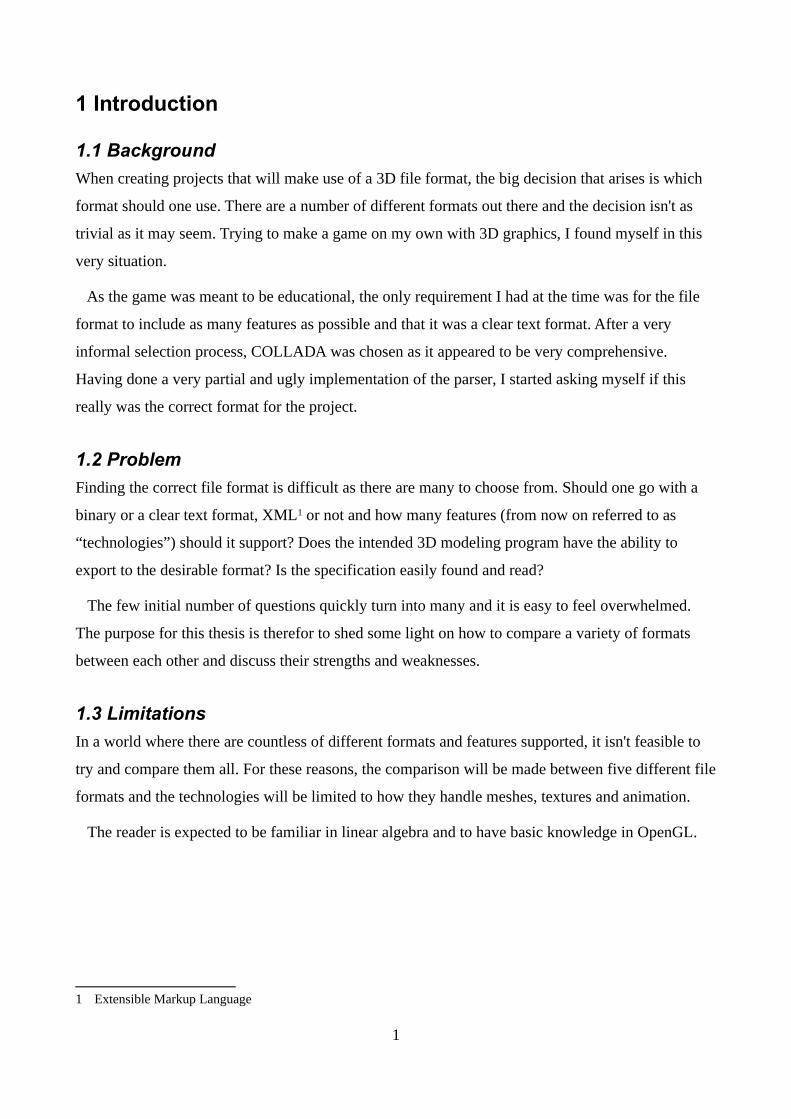
Figure 2.2: The new vertex position at t(0.5) generated by using linear interpolation between the position of the vertices in the two keyframes at t(0) and t(1).
The algorithm to calculate the vertex position P at the time t (which is a value between 0 and 1)
from the keyframe positions P1 and P2 is the following[2]:
4
P=(1−t)⋅P1+t⋅P2
At t=0 the position is P1 and at t=1 it is P2, which is what to be expected.
The problem with linear interpolation is that it doesn't handle movement that consists of curves,
which can be done by using splines. One of the most popular splines is the Bézier curve[1].
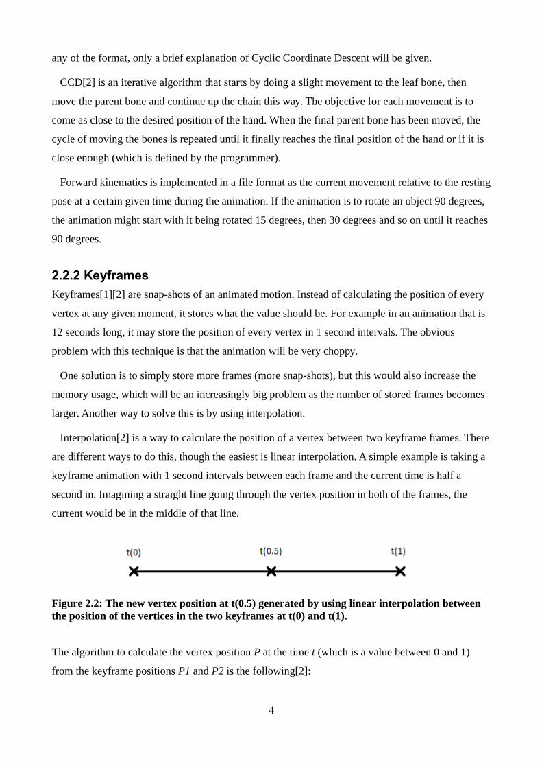
The Bézier curve is calculated by the use of control points, which controls how the curve is bent.
As the Bézier curve belongs to the class of splines which are referred to as approximation splines,
the control points acts like attractor which the curve may or may not pass through, with the
exemption to the first and last control points, which it must pass. Though there is no limitation to
the number of control points used, only the cubic Bézier curve will be explained, as this is the only
one that is supported by any of the evaluated formats. An example of a cubic Bézier is shown in
figure 2.3, where the control points C1 and C4 are the start respectively the end points.
Figure 2.3: A cubic Bézier curve example.
The function to calculate the position p at the time t (which is a number between 0 and 1) is the
following:
p (t)=C1⋅(1−t)3+C2⋅3t(1−t )2+C3⋅3(1−t)t 2+C4⋅t 4
In a file format, keyframe animation may be implemented as simply storing multiple rendering
models in a sequence, where each model is a pose at a certain time. Information about how to
interpolate between each model may also be present.
5

2.2.3 SkinningSkinning[2] is a technique used to deform the mesh of a skeletal model in order to make it represent
the current pose depending on the position of the bones. In order to do this, every vertex needs to be
controlled by one or several bones. In the simplest form, every vertex follows only one bone. This is
called stitching[12]. Stitching works well for basic models, but when the movements gets too large
or as the model gets more detailed, the risk of artifacts being created is increased, as is illustrated in
figure 2.4. The hollow vertices belongs to the white bone and the rest belongs to the dark one.
Figure 2.4: Example of artifacts created by the stitching method.[12]
Allowing multiple bones to be connected to a vertex is called skinning[12]. As some bones affect a
vertex in varying degree, weights are introduced. The sum of all the weights for any vertex must be
1. Rarely more than four bones affect a vertex[2]. Skinning is done in three steps.
The first stage is to transform each bone into the model space, assuming that this is the space the
skin currently is in. This is done by first transforming the root bone into world space by multiplying
it with the position and rotation in the world space. Then multiply the children bone's transform
with the root bone's new transform and continue this multiplication of the parent's world space
transform with each of the children for every bone.
6
The second step is to remove the current pose of the skin, which is often referred to as the rest
post, which is the pose it was exported as; e.g. the resting pose of the skin might be where the knees
are bent which now needs to be unbent. This is done by simply applying the inverse of the
transforms for the resting pose. When this is done, the transforms for the new pose is applied; e.g.
bend the knee in another way.
The third step is to deform the vertex positions according to the bones that affects them.
v '=∑i=1
n
wiM i v
The new position v' for a vertex is derived from the sum of the position v in the current pose
multiplied with the current bone's transform matrix M and the weight it has to that vertex. The
positions of the vertex and the transform matrix for each bone are in the model space.
The implementation of skinning in a file formats may be done by either have the vertex contain a
list comprised of pairs of bone IDs and weights or by letting the bone have a similar list, which has
a reference to the vertex instead the bone IDs.
2.3 MaterialThe simplest case of applying a material to a polygon is texture mapping[1], with the use of a single
texture. This is done by assigning each of the vertices in a polygon a position which points to a
location in a texture. This is a simple way of improving the look of a single polygon and ultimately
the 3D model as a whole, which will be considered as the minimum requirement for this thesis.
2.3.1 MultitexturingMultitexturing[1] is a way to use two or more textures as the surface pattern for a polygon. This
enables the ability to use things like light mapping, which is a way to add static lighting to a texture,
and bump mapping, which is a way to manipulate the normals of a surface. One of the inherent
advantage of using multitexturing in this way is that the modifying picture, e.g. the light map, can
be replaced without having to change the code.
Multitexturing enables also the blending between two textures, which is very useful when doing a
transition between two different ground surfaces. An example of this is a snow covered mountain
peak, which transitions into grass.
The implementation of multitexturing in a file format is usually done by having multiple texture
coordinates be assigned to a vertex.
7
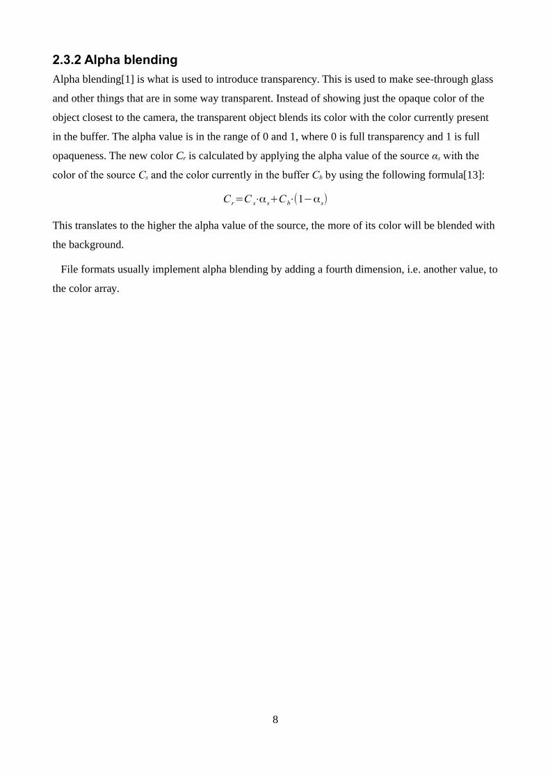
2.3.2 Alpha blendingAlpha blending[1] is what is used to introduce transparency. This is used to make see-through glass
and other things that are in some way transparent. Instead of showing just the opaque color of the
object closest to the camera, the transparent object blends its color with the color currently present
in the buffer. The alpha value is in the range of 0 and 1, where 0 is full transparency and 1 is full
opaqueness. The new color Cr is calculated by applying the alpha value of the source αs with the
color of the source Cs and the color currently in the buffer Cb by using the following formula[13]:
C r=C s⋅αs+Cb⋅(1−αs)
This translates to the higher the alpha value of the source, the more of its color will be blended with
the background.
File formats usually implement alpha blending by adding a fourth dimension, i.e. another value, to
the color array.
8

3 MethodThis chapter will begin with an introduction to the various file formats that are mentioned in this
thesis, so that the reader won't be clueless about the acronyms. This will be followed by how the file
formats were selected and which ones where excluded. Lastly, a description is given of how the
evaluation and comparison was conducted.
3.1 Introduction to the file formatsThe file formats will be introduced by describing how and in what way they store data and if there
are certain things that are worth mentioning (e.g. the MD2 format ability to only make use of one
texture).
3.1.1 B3DB3D[3] is a binary format using little endian with the data described in chunks. A chunk consists of
a header of eight bytes following a data load. The first four bytes of the header are called the tag
which tells what type the chunk is and the last four bytes represent an integer that describe how long
the data load is. An example of a chunk is shown below:
NODE 124
DATA (which in this case, is 124 bytes big)
The BB3D chunk is the root chunk in a B3D file, which has the following definition in the
specification:
BB3D: int version ;file format version: default=1 [TEXS] ;optional textures chunk [BRUS] ;optional brushes chunk [NODE] ;optional node chunk
The first row is the tag, which in this case is BB3D. As can be seen from the comments, the first
field in the data load is an integer that states which version of the file format is used. The enclosing
with brackets ([ ]) states that the element is optional. In this case, all of the three types of chunks
that may be present in the BB3D chunk are optional.
The body of the format is the NODE chunk, which may contain none or several NODE chunks,
which is shown in the specification for it below.
9
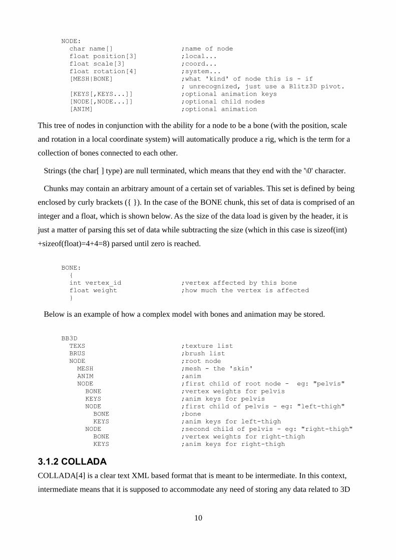
NODE: char name[] ;name of node float position[3] ;local... float scale[3] ;coord... float rotation[4] ;system... [MESH|BONE] ;what 'kind' of node this is - if ; unrecognized, just use a Blitz3D pivot. [KEYS[,KEYS...]] ;optional animation keys [NODE[,NODE...]] ;optional child nodes [ANIM] ;optional animation
This tree of nodes in conjunction with the ability for a node to be a bone (with the position, scale
and rotation in a local coordinate system) will automatically produce a rig, which is the term for a
collection of bones connected to each other.
Strings (the char[ ] type) are null terminated, which means that they end with the '\0' character.
Chunks may contain an arbitrary amount of a certain set of variables. This set is defined by being
enclosed by curly brackets ({ }). In the case of the BONE chunk, this set of data is comprised of an
integer and a float, which is shown below. As the size of the data load is given by the header, it is
just a matter of parsing this set of data while subtracting the size (which in this case is sizeof(int)
+sizeof(float)=4+4=8) parsed until zero is reached.
BONE: { int vertex_id ;vertex affected by this bone float weight ;how much the vertex is affected }
Below is an example of how a complex model with bones and animation may be stored.
BB3D TEXS ;texture list BRUS ;brush list NODE ;root node MESH ;mesh - the 'skin' ANIM ;anim NODE ;first child of root node - eg: "pelvis" BONE ;vertex weights for pelvis KEYS ;anim keys for pelvis NODE ;first child of pelvis - eg: "left-thigh" BONE ;bone KEYS ;anim keys for left-thigh NODE ;second child of pelvis - eg: "right-thigh" BONE ;vertex weights for right-thigh KEYS ;anim keys for right-thigh
3.1.2 COLLADACOLLADA[4] is a clear text XML based format that is meant to be intermediate. In this context,
intermediate means that it is supposed to accommodate any need of storing any data related to 3D
10
modeling, may it be physics or shader data.
The structure of the format starts of with root element called COLLADA, which contains
something that is referred to as libraries and a scene. The scene element contains a reference to the
base of the scene hierarchy which is where the scene starts. The libraries each contain specific sets
of data, e.g. one that holds the mesh information which is called library_geometries, and one that
contains the image information which is called library_images. The rationale for this is to split the
data into specific sections which may then be referenced to.
As COLLADA is meant to be dynamic and intermediate, it takes few things for granted. This is
apparent in the mesh node, where it contains an accessor node, which describes how to load the
floating point numbers into an array of size three, which represents the X, Y and Z axis.
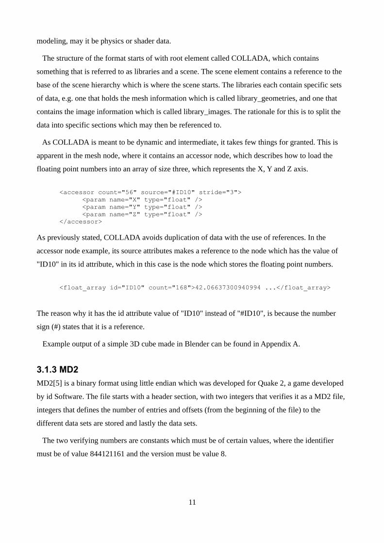
<accessor count="56" source="#ID10" stride="3"><param name="X" type="float" /><param name="Y" type="float" /><param name="Z" type="float" />
</accessor>
As previously stated, COLLADA avoids duplication of data with the use of references. In the
accessor node example, its source attributes makes a reference to the node which has the value of
"ID10" in its id attribute, which in this case is the node which stores the floating point numbers.
<float_array id="ID10" count="168">42.06637300940994 ...</float_array>
The reason why it has the id attribute value of "ID10" instead of "#ID10", is because the number
sign (#) states that it is a reference.
Example output of a simple 3D cube made in Blender can be found in Appendix A.
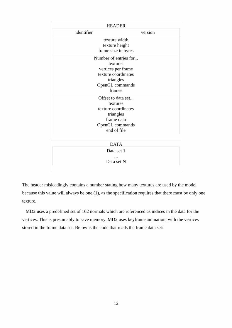
3.1.3 MD2MD2[5] is a binary format using little endian which was developed for Quake 2, a game developed
by id Software. The file starts with a header section, with two integers that verifies it as a MD2 file,
integers that defines the number of entries and offsets (from the beginning of the file) to the
different data sets are stored and lastly the data sets.
The two verifying numbers are constants which must be of certain values, where the identifier
must be of value 844121161 and the version must be value 8.
11
HEADERidentifier version
texture widthtexture height
frame size in bytes
Number of entries for...textures
vertices per frametexture coordinates
trianglesOpenGL commands
frames
Offset to data set...textures
texture coordinatestriangles
frame dataOpenGL commands
end of file
DATAData set 1
...Data set N
The header misleadingly contains a number stating how many textures are used by the model
because this value will always be one (1), as the specification requires that there must be only one
texture.
MD2 uses a predefined set of 162 normals which are referenced as indices in the data for the
vertices. This is presumably to save memory. MD2 uses keyframe animation, with the vertices
stored in the frame data set. Below is the code that reads the frame data set:
12

// Load the framesreader->seek_from_beginning( offset_frames );for( int i = 0 ; i < count_frames ; ++i ){
MD2::Frame frame;float scale[ 3 ] = { reader->read_float(), reader->read_float(),
reader->read_float() };float translate[ 3 ] = { reader->read_float(), reader->read_float(),
reader->read_float() };
frame.name = reader->read_char( 16 );
for( int j = 0 ; j < count_vertices_per_frame ; ++j ){
MD2::Vertex vertex;unsigned char *pos = (unsigned char*) reader->read_char( 3 );
vertex.position.x = pos[ 0 ]*scale[ 0 ] + translate[ 0 ];vertex.position.y = pos[ 1 ]*scale[ 1 ] + translate[ 1 ];vertex.position.z = pos[ 2 ]*scale[ 2 ] + translate[ 2 ];
int index = (int)((unsigned char)*reader->read_char( 1 ));
vertex.normal.x = MD2::NORMALS[ 3*index ];vertex.normal.y = MD2::NORMALS[ 3*index + 1 ];vertex.normal.z = MD2::NORMALS[ 3*index + 2 ];
frame.vertices.push_back( vertex );}
md2->frames.push_back( frame );}
MD2 doesn't provide any instructions on how to interpolate between two frames, though a simple
linear interpolation is probably good enough.
3.1.4 XX[7] is a file format from Microsoft for DirectX version 9 that exists as a little endian binary and as
a clear text format. DirectX version 9 contains a native API to load and display the contents of an X
file. It is possible to load an X file in later version, however it requires some extra steps to convert it
into an sdkmesh[14].
It uses predefined templates[8] to store the data. An example of template definition of a template
can be found below for the Material template:
13
template Material{ < 3D82AB4D-62DA-11CF-AB39-0020AF71E433 > ColorRGBA faceColor; FLOAT power; ColorRGB specularColor; ColorRGB emissiveColor; [...]}
The string enclosed by the angle brackets (< >) is a Universally Unique Identifier (UUID) which is
used in conjunction with the name of the template in order to reference it. The data members are
defined by the type and then its name and they are delimited from each other by a semicolon.
The [...] means that this is an open template, which translates to it being able to have any template
instance inline in the template. If it however looked like this:
[ Material <3D82AB4D-62DA-11CF-AB39-0020AF71E433>]
then it would mean that the template was a restricted template, which may only contain templates of
the kind specified within the brackets. The template is called a closed template if none of them are
present, which means that no templates may be placed inside the template.
Below is an example of an instance of the Material template:
Material material { 0.800000; 0.800000; 0.800000;1.0;; 0.500000; 1.000000; 1.000000; 1.000000;; 0.0; 0.0; 0.0;; }
The first row states this is an instance of the Material template named "material". The second row
represents the ColorRGBA variable named facecolor. ColorRGBA conscists of four floating point
numbers, which are, as previously stated, delimited by semicolons. The second semicolon at the end
on the second row states that the ColorRGBA variable is now done.
Instead of duplicating data, an instance of a template may be referenced by having its name,
UUID or borth placed with curly brackets ({ }). The reference to the instance of the Material
template above would like {material}, {<Material's UUID>} or {material <Materials UUID>}.
Example output of a simple 3D cube made in Blender can be found in Appendix A.
3.1.5 MDDMDD[6] is a binary format that uses big endian. It is a very simple format that is aimed for storing
14

animated meshes which have the following structure:
int number_of_framesint number_of_pointsfloat time_per_frame[number_of_frames]float points[number_of_frames][number_of_points][axis]
As this format was skipped, no more in depth introduction will be made.
3.1.6 X3DX3D[9] is a clear text format using XML to structure the data. It is a very feature rich format that
supports not only the storing of a 3D scene, but also e.g. interaction (i.e. user input) and audio. As
this format was skipped, no more in depth introduction will be made. An example output of a
simple 3D cube made in Blender can, however, be found in Appendix A.
3.1.7 XSIXSI[10] is a clear text format from Softimage Co. that uses templates to store its data. The
specification of templates is similar to the one in the X file format, as there exists a definition of the
templates which are then used to parse the instances of them. As this format was skipped, no more
in depth introduction will be made. An example output of a simple 3D cube made in Blender can,
however, be found in Appendix A.
3.2 Choice of file formatsThe selection of file formats was initially based on the export capabilities of the 3D modeling
software Blender. The reasoning behind the choice to work with and only with Blender was:
1. Keeping it simple. As I didn't have any real experience with 3D modeling software and due
to the limited time of this thesis.
2. The ability to export the same project to every format.
3. Assuming the exporters are equally good/bad, the comparison would be somewhat fair.
The choosing of the formats was then based on what they supported (textures and animation in this
case) and if there appeared to be some specification available. Although clear text formats were
supposed to be favored because it would be easier to understand what a section of data contained, it
didn't really interfere with the selection.
The file formats initially chosen were COLLADA2, MD2, XSI, X3D and MDD. All formats
2 Version 1.4.x
15

except for XSI were under a free license, but since Blender had the capability to export to it, this
wasn't considered as a big concern at the time.
The proprietary license of XSI meant that there weren't any official version of the specification
available and there were no known complete versions at the time. Not wanting to spend time
creating a parser which in the worst case would adhere to an incorrect specification, it was decided
to replace the file format with another.
Reiterating the same process as before, while emphasizing there being a seemingly complete
specification, the X file format was chosen.
While looking closer at the specification of the MDD format, it became evident that though it had
support for keyframe animation, it didn't have support for textures. As some kind of support for
textures was important, it was decided that it would be scratched as well.
Replacing the format proved to be slightly difficult, as there weren't any suitable candidates left
that Blender's exporter could handle. This meant that a format outside of the exporter's capabilities
had to be found, which allowed for more freedom in the choice. Looking at the irrLicht Engine3
project for inspiration, B3D was chosen. The specification was freely available and well written and
examples of saved 3D models could be easily found.
In the late phases of the thesis, it was decided that X3D would be skipped as well, as the reading
of the specification proved to be more difficult than anticipated. Though a parser was created using
the CodeSynthesis XSD4 project with the X3D's XSD files, it didn't help with the understanding of
the specification as the generated parser wasn't particularly human-readable.
3.3 How to evaluate and compareIn order to get more experience with the formats, it was decided that a parser for each of the formats
would be constructed. The parsers were to be written in C++, as the specifications tends to have
example code written in C or C++ and the need to translate the data types would be unnecessary
(for instance, unsigned integers doesn't exist in Java).
The initial thought was to have the parsers transform the parsed data into an intermediate format,
so that the process of turning it into OpenGL code could be simplified. Due to uncertainties on how
to translate the different ways the file formats store data into this intermediate format, it was
skipped and it was decided that the OpenGL code generation would be done separately for each of
the formats.
3 A free and open source 3D engine (http://irrlicht.sourceforge.net/)4 http://www.codesynthesis.com/products/xsd/
16

Recognizing that the time for this thesis was limited and not knowing how much work it would
take to make a parser for any of the formats, it was decided that if there weren't enough time, only a
theoretical study would be done. The reasoning for this decision was that having done one or more
parsers, it would be easier to imagine writing a parser by just looking at the specification.
17
4 ComparisonThe first part of this chapter will describe how the evaluation process of each of the file formats was
conducted and the last part will try to make a comparison based on the results of the evaluations.
4.1 Parser implementationsAs stated in section 3.3, a parser was to be constructed for each of the formats in order to get more
familiar and experienced with the formats.
In order to ease the implementation, the parsers were separated by design, joined by an interface
that determines which parser to use according to the file extension of the file and that returns a
Graphic object, which contains the converted OpenGL code.
Every parser implements the method parse( std::string filepath ), which returns the data structure
that corresponds to the file format. A visualizer class is then able to convert the data structure into
OpenGL code. In order to save time, a visualizer for each of the formats was constructed (due to
further lack of time, this was only done for COLLADA and MD2).
Though the parsers are separated from each other, shared tools were constructed in order to avoid
duplication of code and to save time. As the problem with different endianess became apparent
during the implementation of the MD2Parser, the BinaryReader was constructed to handle any
needed conversion between the endianess in the file format and the computer system (more details
can be found in section 4.1.2).
4.1.1 COLLADAA COLLADA parser was made, which proved to be uncomplicated. The specification was
structured in such a way that made it easy to implement. The attributes are clearly specified with
types, if they are optional and whether there is a default value. Child nodes are listed and the
number of occurrences can be easily read. At the end of each node specification, an example can
most of the times be found of how the node might look like in the file and also how to use the data
it contains.
Not wanting to spend a lot of time creating an XML parser from scratch, a search for one already
implemented was conducted. This search wasn't done in any particular way, the criteria was that it
would be based on the zlib/libpng license5 or similar (as this is the expected license for this project)
5 http://www.opensource.org/licenses/zlib-license.php
18
and that it would be simple and fast to use. IrrXML6 fulfilled all of the above requirements and was
therefor chosen.
Not having to worry about the XML parsing, the rest of the implementation was trivial. For each
node, a method was implemented that parsed and returned a corresponding data structure with the
parsed data. This split the parser into smaller pieces, which made it more maintainable and
simplified the implementation. Below is the code to parse an accessor node (an example of how this
node looks like was shown in section 3.1.2).
const Accessor* COLLADAParser::parse_accessor( irr::io::IrrXMLReader *reader ) const
{Accessor *acc = new Accessor();bool isNotDone = true;
const char* offset = reader->getAttributeValue( "offset" );const char* stride = reader->getAttributeValue( "stride" );
// count and source must be presentacc->count =
(unsigned int) atoi( reader->getAttributeValue( "count" ) );acc->source = reader->getAttributeValue( "source" );
// offset and stride may not be present, check if they were foundacc->offset = offset ? (unsigned int) atoi( offset ) : acc->offset;acc->stride = stride ? (unsigned int) atoi( stride ) : acc->stride;
while( isNotDone && reader && reader->read() ){
switch( reader->getNodeType() ){case EXN_ELEMENT:
if( !strcmp( "param", reader->getNodeData() ) )acc->params.push_back( parse_param( reader ) );
break;case EXN_ELEMENT_END:
if( !strcmp( "accessor", reader->getNodeData() ) )isNotDone = false;
break;default: break;}
}return acc;
}
This function is called when the starting tag for accessor (“<accessor>”) is parsed. Any attributes
that may be present in this tag is then parsed. In the case of the accessor node, the count and source
attributes must be present, whereas the offset and stride doesn't have to. If an attribute that is not
6 Part of the irrLicht project, it is a stand alone free and open source XML parser (http://www.ambiera.com/irrxml/)
19

present in the current tag, then the irrXMLReader will return null (otherwise a valid pointer to a
const char structure), which means that we need to check if the pointer to the offset and the stride is
0 or not and act accordingly.
As the optional attributes may have a default value (e.g. 0 for offset), these needs to be set if the
attributes aren't found in the tag. This was done by having the data structure initialize the values of
these variables to the default value and merely set the variable's value to the current one if the
pointer of the parsed data was null. Below is the code for the data structure for the accessor node.
#include <string>#include "Param.h"
struct Accessor{
Accessor(): offset( 0 ), // Default according to specstride( 1 ) // Default according to spec
{}
// Attributesunsigned int count;unsigned int offset;std::string source;unsigned int stride;
// Child elementsstd::vector<const Param*> params;
};
When the attributes have been parsed, it is time to parse the child nodes. As the specification doesn't
state in which order the nodes are placed, a loop was constructed in which a check is made for each
possible child node and then parse them if they are discovered. As there may be multiple
occurrences of the param node, a vector is used to store the parsed param nodes. The loop ends if
the end-tag for accessor is parsed.
A simple viewer was also created, which made it possible to verify that the parsed data was
correct. Figure 4.1 shows a 3D model created in Google SketchUp being displayed by the viewer.
20
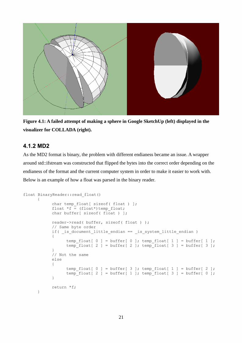
Figure 4.1: A failed attempt of making a sphere in Google SketchUp (left) displayed in the
visualizer for COLLADA (right).
4.1.2 MD2As the MD2 format is binary, the problem with different endianess became an issue. A wrapper
around std::ifstream was constructed that flipped the bytes into the correct order depending on the
endianess of the format and the current computer system in order to make it easier to work with.
Below is an example of how a float was parsed in the binary reader.
float BinaryReader::read_float(){
char temp_float[ sizeof( float ) ];float *f = (float*)temp_float;char buffer[ sizeof( float ) ];
reader->read( buffer, sizeof( float ) );// Same byte orderif( _is_document_little_endian == _is_system_little_endian ){
temp_float[ 0 ] = buffer[ 0 ]; temp_float[ 1 ] = buffer[ 1 ];temp_float[ 2 ] = buffer[ 2 ]; temp_float[ 3 ] = buffer[ 3 ];
}// Not the sameelse{
temp_float[ 0 ] = buffer[ 3 ]; temp_float[ 1 ] = buffer[ 2 ];temp_float[ 2 ] = buffer[ 1 ]; temp_float[ 3 ] = buffer[ 0 ];
}
return *f;}
21
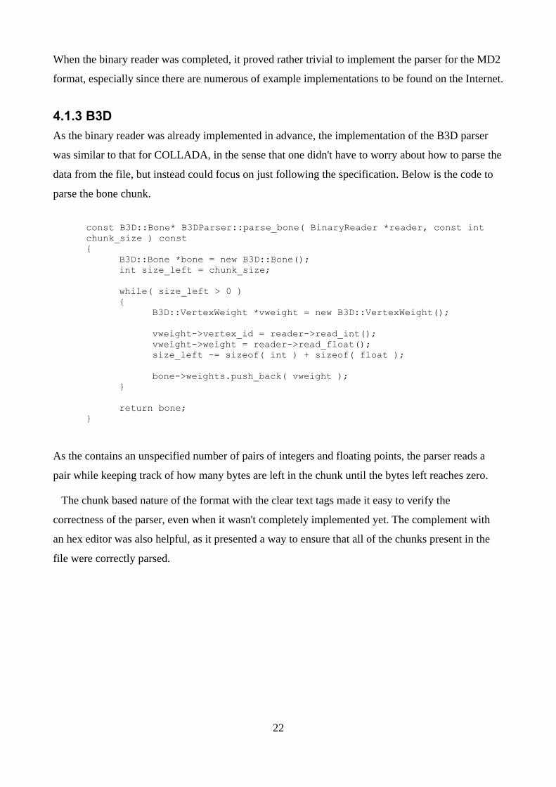
When the binary reader was completed, it proved rather trivial to implement the parser for the MD2
format, especially since there are numerous of example implementations to be found on the Internet.
4.1.3 B3DAs the binary reader was already implemented in advance, the implementation of the B3D parser
was similar to that for COLLADA, in the sense that one didn't have to worry about how to parse the
data from the file, but instead could focus on just following the specification. Below is the code to
parse the bone chunk.
const B3D::Bone* B3DParser::parse_bone( BinaryReader *reader, const int chunk_size ) const{
B3D::Bone *bone = new B3D::Bone();int size_left = chunk_size;
while( size_left > 0 ){
B3D::VertexWeight *vweight = new B3D::VertexWeight();
vweight->vertex_id = reader->read_int();vweight->weight = reader->read_float();size_left -= sizeof( int ) + sizeof( float );
bone->weights.push_back( vweight );}
return bone;}
As the contains an unspecified number of pairs of integers and floating points, the parser reads a
pair while keeping track of how many bytes are left in the chunk until the bytes left reaches zero.
The chunk based nature of the format with the clear text tags made it easy to verify the
correctness of the parser, even when it wasn't completely implemented yet. The complement with
an hex editor was also helpful, as it presented a way to ensure that all of the chunks present in the
file were correctly parsed.
22
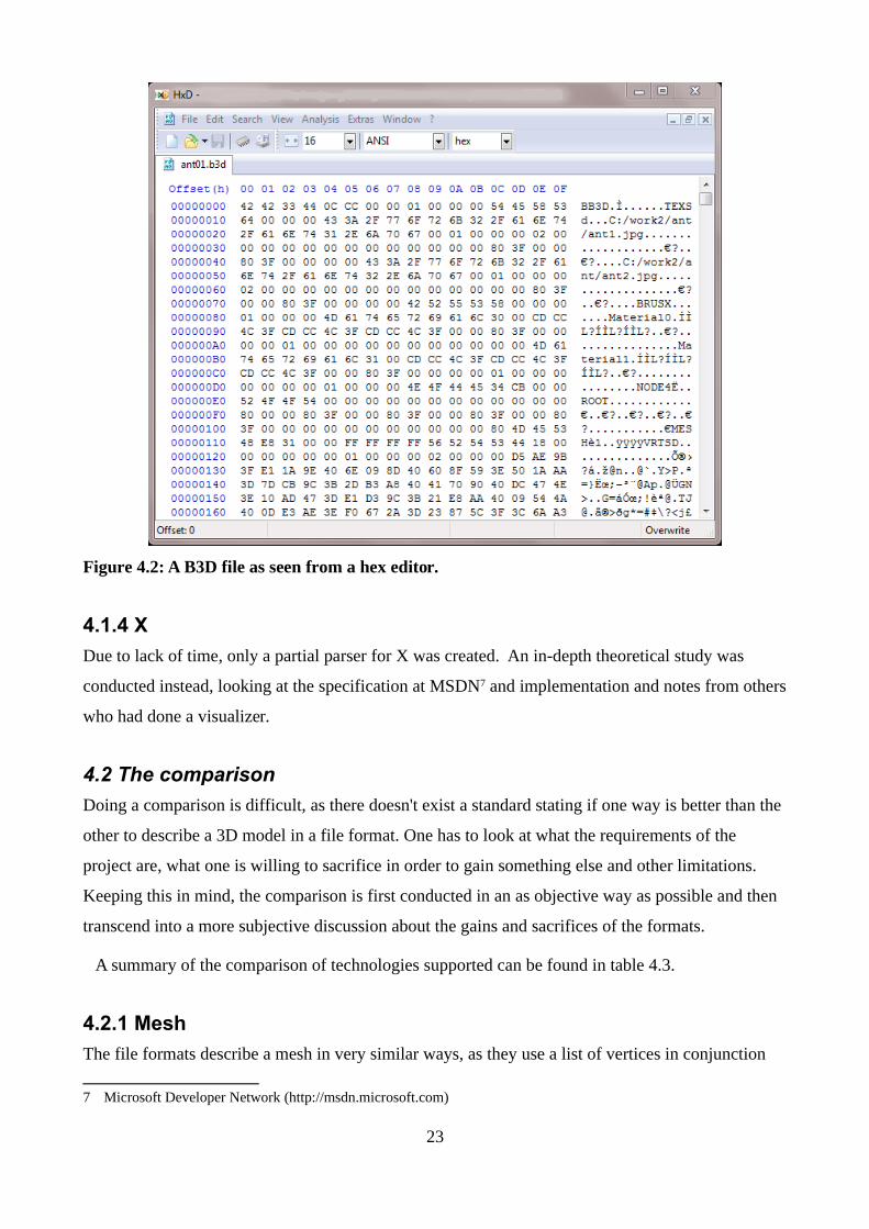
Figure 4.2: A B3D file as seen from a hex editor.
4.1.4 XDue to lack of time, only a partial parser for X was created. An in-depth theoretical study was
conducted instead, looking at the specification at MSDN7 and implementation and notes from others
who had done a visualizer.
4.2 The comparisonDoing a comparison is difficult, as there doesn't exist a standard stating if one way is better than the
other to describe a 3D model in a file format. One has to look at what the requirements of the
project are, what one is willing to sacrifice in order to gain something else and other limitations.
Keeping this in mind, the comparison is first conducted in an as objective way as possible and then
transcend into a more subjective discussion about the gains and sacrifices of the formats.
A summary of the comparison of technologies supported can be found in table 4.3.
4.2.1 MeshThe file formats describe a mesh in very similar ways, as they use a list of vertices in conjunction
7 Microsoft Developer Network (http://msdn.microsoft.com)
23
with a list of indices to describe polygons. The difference lies in how they split the mesh model.
MD2 uses a single mesh to describe the model while the others may also split the mesh model into
sub meshes.
4.2.2 AnimationMD2[5] and COLLADA[4] only supports keyframe animation, though they differ in the
implementation. Whereas MD2 stores a list of vertices for each frame, COLLADA instead uses
sampler that describes how to manipulate the mesh using splines depending on the time that has
elapsed.
B3D[3] and X[11] only supports forward kinematics with no significant difference in the
implementation.
Skinning is supported in COLLADA, B3D and X, as vertex weights are present. In addition to
this, the COLLADA specification contains information on how to perform skinning with an
algorithm and how to use the information stored in relevant nodes.
4.2.3 MaterialsMD2 supports no alpha blending and only one texture per model. COLLADA and B3D both
supports multitexturing and alpha blending.
X supports several textures and alpha blending, but it doesn't, however, include multitexturing
however.
4.2.4 File structureXML is a very neat format, as it is a human-readable format and as there exist numerous freely
available parsers for it. Translating it to data structures proved to be very easy and the process of
creating the COLLADA parser was very straight forward.
Binary formats are really easy to work with, as they tend to be compact and one doesn't have to
worry about spaces between the data. They are, for obvious reasons, not human-readable which is a
problem when verifying that the parser works correctly. The different endianesses is an issue, but it
is maintainable by making a reader that handles the conversion. Binary formats will most likely take
less time to parse, as the information is already in a format in which can be used (i.e. an integer is
not stored as a string, but as four bytes). A simple test was conducted where a varying amount of
floating points are saved in a clear text and as a binary file and a parser was made to read and
convert the data. Table 4.1 shows the time needed to parse for each of the readers. The difference is
24

noticeable when a large amount of numbers are parsed, but gets less visible as the amount of
numbers decreases. This is probably due to file size, as the binary file is 4kB in size in the first test
and 3907kB in the second, whereas the clear text file is 7kB in size in the first test and 6929kB in
the second. The source code and information about this test can be found Appendix B.
Number of floats Clear text (in seconds) Binary (in seconds)
1 000 (run #1) 0.070 0.054
1 000 (run #2) 0.061 0.072
1 000 (run #3) 0.075 0.064
1 000 average 0.069 0.063
1 000 000 (run #1) 0.680 0.178
1 000 000 (run #2) 0.674 0.166
1 000 000 (run #3) 0.698 0.165
1 000 000 average 0.684 0.170Table 4.1 The time needed to parse binary and clear text files.
Although the clear text format used in the X file format requires a custom parser, the uniform
structure of the templates should simplify the implementation.
4.2.5 SpecificationCOLLADA has a complete official specification that contains not only a description of every node,
it also contains valuable examples on how one should use the data. It is very easy to get into and
one doesn't have to spend a lot of time reading the specification before one can begin the
implementation.
Although no official MD2 specification was found, there are still a large number of sources that
contain not only information about the file format but also how to use it in OpenGL.
B3D's specification is easily found and it is very easy to read. It provides information on how to
translate the chunks into data structures and it contains many valuable comments.
The documentation for the X format at MSDN provides basic information about the templates. In
most cases, it just provides the structure for a template without stating how the values were meant to
be used. However, as in the case of MD2, there are other sources that contain useful comments and
some examples on how to use the data.
25

4.2.6 File sizeUsing the example project files8 for Blender version 2.49, the size of the files generated by the
exporters is measured, which is shown in table 4.2. MD2 is not present in the table, as the exporter
was unable to produce any output due to the format's limitation in how many vertices that can be
stored.
Test file COLLADA (in kB) B3D (in kB) X (in kB)
dolphin 2168 802 N/A
softbody_basics 57 22 169
monkey_cornelius 402 161 4898Table 4.2 Exported file sizes of test projects.
B3D appears to produce files of smaller sizes than COLLADA and X, but it is difficult to verify that
the output actually contains all of the necessary data as it is a binary format. In the case the dolphin
test file, the exporter for the X file format failed to produce a file that contained all of the data (only
a single mesh was present without any animation information). A possible explanation for the
smaller sizes of the COLLADA files compared to the X files is that COLLADA is able to reuse data
in a more efficient way, but it may also be because the COLLADA exporter was unable transport
the whole model.
A screenshot of the monkey_cornelius project is found in figure 4.3.
Figure 4.3: A screenshot of monkey_cornelius.
8 http://download.blender.org/demo/test/test249.zip
26

4.3 DiscussionThe discussion will begin with a subjective evaluation of each of the formats and end with a
motivation of when and where the format could be used. An overview of the technologies supported
in the formats is shown in table 4.3.
COLLADA MD2 B3D X
Binary x x
Animation
Keyframe x x
Forward Kinematics x x
Skinning x x x
Material
Multitexturing x x
Alpha blending x x xTable 4.3: An overview of the technologies supported in the file formats.
4.3.1 COLLADAThe sacrifice with COLLADA is that the format is very big and the files generated tends to be quite
large. COLLADA also supports many different ways to describe the same thing. Retrieving a single
mesh requires the whole document to be parsed in order to ensure that all the data is available. This
is because of the format's ability to make references that in turn might point to another reference
until it finally points to the actual data.
The dynamic nature of the format, which gives it the ability to split things up into smaller pieces,
makes it harder to predict what the output might look like from any 3D modeling software. For
instance, Blender's exporter tends to split meshes into sub meshes whereas Google SketchUp's tries
to only export a single mesh. Though this isn't a problem while parsing the file, it becomes an issue
when trying to use the data in order to visualize it. One has to first loop through the chain of
references until one reaches the actual data holding node. This means that the work of processing
the data will take some time which adds to the time required to load the model.
The advantage of COLLADA is that it contains (or at least might contain) a lot of advanced
features, such as physics and shaders. This makes it more likely that one shouldn't have to change
formats due to lack of support of a certain feature, which may save a lot of time.
27

4.3.2 MD2MD2 is a small and simple format that doesn't require much time to either implement or understand.
As implementations can be found in C (and probably lots of other languages) the time needed for
implementations is further reduced.
Its disadvantage lies in its simplicity. Bones, multitexturing and/or the ability to use more than one
texture per model are things that one might want to make use of, which would mean that a new
format would have to be chosen.
4.3.3 B3DB3D is a format made to be easy to use and extensible, where planned future features include
camera, lighting and sprites[3]. As it is chunk-based, only support for new chunks needs to be added
in order to update the parser.
4.3.4 XThe X format is a very dynamic format which supports a lot of things. The lack of official
documentation is a concern, as one is pretty much dependent on other sources to gain the much
needed comments. This might sound like the case with MD2, but there is a difference. As the X
format is a lot larger, finding a source that completely describes the format might prove difficult.
There are quite a few issues with the implementation of the format. The first one being that no
root template exist as the first template in the file. The second problem is the open templates. An
open template is a template that may contain other templates. This is similar to COLLADA and
B3D, with the exception that there exists templates that may contain any other template, instead of a
selected few. How does one implement this? How should this be used? With more time, these
question probably could have been answered, which is worth mentioning.
4.3.5 Ending notesWith this in mind, it is time to make a decision of when to use the formats, which will be based
upon the features supported and the work needed to make a parser.
COLLADA is a very big and complex format which supports a lot of features. Though the
specification is a big help, the numerous ways of representing a model with the format requires a lot
of work with the implementation of the parser, which makes the format suitable for bigger projects
that requires the features supported.
MD2 is a very small and simple format which requires very little effort to implement and use. The
28
supported features are however limited, which probably will be less than what is required in later
stages of a project. This makes MD2 suitable for projects that doesn't require many features besides
basic animation and doesn't need to support more than one texture.
B3D is a simple and extendible format which supports a fair number features. The specification is
complete with a number of useful comments which simplifies the implementation. The format is
suited for projects that are of medium to large in size.
X is a complex format which supports less features than COLLADA, but more than B3D, e.g.
bézier patches. The specification is difficult to read and it is in some cases incomplete. The open
templates makes the implementation of the parser non-trivial, which makes this format mostly
suitable for large projects, as the time needed to make an implementation will most likely take a lot
of time. It is though worth noting that if DirectX version 9 is to be used in the project, the use of the
format will probably be a lot simpler, as the built-in API9 then can be used.
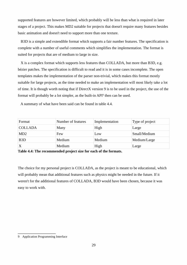
A summary of what have been said can be found in table 4.4.
Format Number of features Implementation Type of project
COLLADA Many High Large
MD2 Few Low Small/Medium
B3D Medium Medium Medium/Large
X Medium High LargeTable 4.4: The recommended project size for each of the formats.
The choice for my personal project is COLLADA, as the project is meant to be educational, which
will probably mean that additional features such as physics might be needed in the future. If it
weren't for the additional features of COLLADA, B3D would have been chosen, because it was
easy to work with.
9 Application Programming Interface
29

5 ConclusionsAlthough it wasn't a requirement in this study, creating a visualizer for each of the formats would
have resulted in a better understanding of the formats. This was especially true in the case of
COLLADA, where the problems lied more in how to use the data parsed rather than in the parsing
of the data. This would have resulted in more time having to be allocated for each format, which
would have made it necessary to reduce the number of formats to evaluate.
When considering a format, doing a thorough and in-depth study of the specification may prove to
save a lot of time. A week was spent on trying to create a parser for X3D, which is time that could
have been spent on evaluating another format or as extra time for the other formats, due to its
specification being very difficult to read. The same rational can be made for the MDD and the XSI
format, which needed to be replaced in the middle of the thesis, which probably resulted in days
work wasted trying to find other formats.
5.1 Future workMaking the implementation a requirement with both a parser and a visualizer would have enabled
the comparison of the time needed to import a model. This type of comparison would have been
very interesting to do with a big and complex model, as it would most likely show a distinct
difference between a format that is specialized for speed, like MD2, and a format which is made to
be intermediate, like COLLADA.
If possible, it would be interesting to see how much the output of the exporters of two different
3D modelling programs differs, as this would entail if a format is given a disadvantage because of
the choice of program.
30
Bibliography[1] Ingemar Ragnemalm, Polygons Feel No Pain, third edition, 2010
[2] Steve Rabin, Introduction to Game Development, second edition, Charles River Media, 2009
[3] Blitz Research Ltd , "Blitz3d file format V0.01",
http://www.blitzbasic.co.nz/sdkspecs/sdkspecs/b3dfile_specs.txt, June 2011
[4] M. Barnes and E. L. Finch, COLLADA – Digital Asset Schema Release 1.4.1, second edition,
2008
[5] D. Henry, "MD2 file format specifications (Quake 2's models)"
http://tfc.duke.free.fr/coding/md2-specs-en.html, June 2011
[6] M. Wilson, N/A http://www.ef9.com/ef9/PO1.5/LW/PointOven_lw.html, June 2011
[7] K. Ditchburn, “Direct3D 3D Models“, http://www.toymaker.info/Games/html/3d_models.html,
June 2011
[8] Microsoft, "Templates (Windows)", http://msdn.microsoft.com/en-
us/library/bb173021%28v=vs.85%29.aspx, June 2011
[9] Web3D Consortium, "What is X3D?" http://www.web3d.org/about/overview/, June 2011
[10] Avid Technology, Inc, "Softimage XSI File Format v3.0",
http://www.bz2md.com/fishdotxsi/xsi.htm#568262, June 2011
[11] Keith Ditchburn, "Load X Hierarchy",
http://www.toymaker.info/Games/html/load_x_hierarchy.html, June 2011
[12] Ingemar Ragnemalm, So how can we make them scream?, third edition, 2008
[13] R. S. Wright, Jr., N. Haemel, G. Sellers, B. Lipchak, OpenGL SuperBible: Comprehensive
Tutorial and Reference, fifth edition, Addison-Wesley Professional, 2010
[14] K. Ditchburn, "Direct3D 3D Models",
http://www.toymaker.info/Games/html/3d_models.html#d10, August 2011
31

Appendix A Example files describing a simple cube
A.1 COLLADA<?xml version="1.0" encoding="UTF-8" standalone="no" ?><COLLADA xmlns="http://www.collada.org/2005/11/COLLADASchema" version="1.4.1"> <asset> <contributor> <authoring_tool>Google SketchUp 8.0.3117</authoring_tool> </contributor> <created>2010-11-20T20:12:33Z</created> <modified>2010-11-20T20:12:33Z</modified> <unit meter="0.02539999969303608" name="inch" /> <up_axis>Z_UP</up_axis> </asset> <library_visual_scenes> <visual_scene id="ID1"> <node name="SketchUp"> <instance_geometry url="#ID2"> <bind_material> <technique_common> <instance_material symbol="Material2" target="#ID3"> <bind_vertex_input semantic="UVSET0" input_semantic="TEXCOORD" input_set="0" /> </instance_material> <instance_material symbol="Material3" target="#ID8"> <bind_vertex_input semantic="UVSET0" input_semantic="TEXCOORD" input_set="0" /> </instance_material> </technique_common> </bind_material> </instance_geometry> </node> </visual_scene> </library_visual_scenes> <library_geometries> <geometry id="ID2"> <mesh> <source id="ID5"> <float_array id="ID10" count="168">42.06637300940994 68.91902768970225 0 -24.86276084885776 -39.37458573056625 0 -24.86276084885776 68.91902768970225 0 42.06637300940994 -39.37458573056625 0 42.06637300940994 -39.37458573056625 0 42.06637300940994 68.91902768970225 0 -24.86276084885776 -39.37458573056625 0 -24.86276084885776 68.91902768970225 0 -24.86276084885776 68.91902768970225 0 -24.86276084885776 -39.37458573056625 0 42.06637300940994 68.91902768970225 0 42.06637300940994 -39.37458573056625 0 -24.86276084885776 68.91902768970225 38.97637795275591 -24.86276084885776 -39.37458573056625 0 -24.86276084885776 -39.37458573056625 38.97637795275591 -24.86276084885776 68.91902768970225 0 -24.86276084885776 68.91902768970225 0 -24.86276084885776 68.91902768970225 38.97637795275591 -24.86276084885776 -39.37458573056625 0 -24.86276084885776 -39.37458573056625 38.97637795275591 -24.86276084885776 -39.37458573056625 38.97637795275591 -24.86276084885776 68.91902768970225 38.97637795275591 -24.86276084885776 68.91902768970225 38.97637795275591 42.06637300940994 68.91902768970225 0 -24.86276084885776 68.91902768970225 0 42.06637300940994 68.91902768970225 38.97637795275591 42.06637300940994 68.91902768970225 38.97637795275591 -24.86276084885776 68.91902768970225 38.97637795275591 42.06637300940994 68.91902768970225 0 -24.86276084885776 68.91902768970225 0 42.06637300940994 68.91902768970225 38.97637795275591 42.06637300940994 68.91902768970225 0 42.06637300940994 -39.37458573056625
32

38.97637795275591 42.06637300940994 -39.37458573056625 0 42.06637300940994 68.91902768970225 38.97637795275591 42.06637300940994 68.91902768970225 38.97637795275591 42.06637300940994 68.91902768970225 0 42.06637300940994 -39.37458573056625 38.97637795275591 42.06637300940994 -39.37458573056625 0 42.06637300940994 -39.37458573056625 38.97637795275591 42.06637300940994 -39.37458573056625 38.97637795275591 -24.86276084885776 -39.37458573056625 0 42.06637300940994 -39.37458573056625 0 -24.86276084885776 -39.37458573056625 38.97637795275591 -24.86276084885776 -39.37458573056625 38.97637795275591 42.06637300940994 -39.37458573056625 38.97637795275591 -24.86276084885776 -39.37458573056625 0 42.06637300940994 -39.37458573056625 0 42.06637300940994 -39.37458573056625 38.97637795275591 -24.86276084885776 68.91902768970225 38.97637795275591 -24.86276084885776 -39.37458573056625 38.97637795275591 42.06637300940994 68.91902768970225 38.97637795275591 42.06637300940994 68.91902768970225 38.97637795275591 42.06637300940994 -39.37458573056625 38.97637795275591 -24.86276084885776 68.91902768970225 38.97637795275591 -24.86276084885776 -39.37458573056625 38.97637795275591</float_array> <technique_common> <accessor count="56" source="#ID10" stride="3"> <param name="X" type="float" /> <param name="Y" type="float" /> <param name="Z" type="float" /> </accessor> </technique_common> </source> <source id="ID6"> <float_array id="ID11" count="168">0 0 -1 0 0 -1 0 0 -1 0 0 -1 -0 -0 1 -0 -0 1 -0 -0 1 -0 -0 1 0 0 0 0 0 0 0 0 0 0 0 0 -1 0 0 -1 0 0 -1 0 0 -1 0 0 1 -0 -0 1 -0 -0 1 -0 -0 1 -0 -0 0 0 0 0 0 0 -0 1 0 -0 1 0 -0 1 0 -0 1 0 0 -1 -0 0 -1 -0 0 -1 -0 0 -1 -0 0 0 0 1 0 0 1 0 0 1 0 0 1 0 0 -1 -0 -0 -1 -0 -0 -1 -0 -0 -1 -0 -0 0 0 0 -0 -1 -0 -0 -1 -0 -0 -1 -0 -0 -1 -0 0 1 0 0 1 0 0 1 0 0 1 0 0 0 1 0 0 1 0 0 1 0 0 1 -0 -0 -1 -0 -0 -1 -0 -0 -1 -0 -0 -1</float_array> <technique_common> <accessor count="56" source="#ID11" stride="3"> <param name="X" type="float" /> <param name="Y" type="float" /> <param name="Z" type="float" /> </accessor> </technique_common> </source> <vertices id="ID7"> <input semantic="POSITION" source="#ID5" /> <input semantic="NORMAL" source="#ID6" /> </vertices> <triangles count="24" material="Material2"> <input offset="0" semantic="VERTEX" source="#ID7" /> <p>0 1 2 1 0 3 4 5 6 7 6 5 12 13 14 13 12 15 16 17 18 19 18 17 22 23 24 23 22 25 26 27 28 29 28 27 31 32 33 32 31 34 35 36 37 38 37 36 40 41 42 41 40 43 44 45 46 47 46 45 48 49 50 49 48 51 52 53 54 55 54 53</p> </triangles> <lines count="12" material="Material3"> <input offset="0" semantic="VERTEX" source="#ID7" /> <p>8 9 10 8 11 10 9 11 9 20 21 20 8 21 30 21 10 30 39 30 11 39 20 39</p> </lines> </mesh> </geometry> </library_geometries> <library_materials> <material id="ID3" name="material_0"> <instance_effect url="#ID4" /> </material>
33

<material id="ID8" name="edge_color000255"> <instance_effect url="#ID9" /> </material> </library_materials> <library_effects> <effect id="ID4"> <profile_COMMON> <technique sid="COMMON"> <lambert> <diffuse> <color>1 0.3294117647058824 0.3294117647058824 1</color> </diffuse> </lambert> </technique> </profile_COMMON> </effect> <effect id="ID9"> <profile_COMMON> <technique sid="COMMON"> <constant> <transparent opaque="A_ONE"> <color>0 0 0 1</color> </transparent> <transparency> <float>1</float> </transparency> </constant> </technique> </profile_COMMON> </effect> </library_effects> <scene> <instance_visual_scene url="#ID1" /> </scene></COLLADA>
A.2 Xxof 0303txt 0032
template VertexDuplicationIndices { <b8d65549-d7c9-4995-89cf-53a9a8b031e3> DWORD nIndices; DWORD nOriginalVertices; array DWORD indices[nIndices];}template XSkinMeshHeader { <3cf169ce-ff7c-44ab-93c0-f78f62d172e2> WORD nMaxSkinWeightsPerVertex; WORD nMaxSkinWeightsPerFace; WORD nBones;}template SkinWeights { <6f0d123b-bad2-4167-a0d0-80224f25fabb> STRING transformNodeName; DWORD nWeights; array DWORD vertexIndices[nWeights]; array float weights[nWeights]; Matrix4x4 matrixOffset;
34
}
Frame RootFrame {
FrameTransformMatrix { 1.000000,0.000000,0.000000,0.000000, 0.000000,1.000000,0.000000,0.000000, 0.000000,0.000000,-1.000000,0.000000, 0.000000,0.000000,0.000000,1.000000;; } Frame Cube {
FrameTransformMatrix { 1.000000,0.000000,0.000000,0.000000, 0.000000,1.000000,0.000000,0.000000, 0.000000,0.000000,1.000000,0.000000, 0.000000,0.000000,0.000000,1.000000;; }Mesh {24;1.000000; 1.000000; -1.000000;,1.000000; -1.000000; -1.000000;,-1.000000; -1.000000; -1.000000;,-1.000000; 1.000000; -1.000000;,1.000000; 1.000000; 1.000000;,-1.000000; 1.000000; 1.000000;,-1.000000; -1.000000; 1.000000;,1.000000; -1.000000; 1.000000;,1.000000; 1.000000; -1.000000;,1.000000; 1.000000; 1.000000;,1.000000; -1.000000; 1.000000;,1.000000; -1.000000; -1.000000;,1.000000; -1.000000; -1.000000;,1.000000; -1.000000; 1.000000;,-1.000000; -1.000000; 1.000000;,-1.000000; -1.000000; -1.000000;,-1.000000; -1.000000; -1.000000;,-1.000000; -1.000000; 1.000000;,-1.000000; 1.000000; 1.000000;,-1.000000; 1.000000; -1.000000;,1.000000; 1.000000; 1.000000;,1.000000; 1.000000; -1.000000;,-1.000000; 1.000000; -1.000000;,-1.000000; 1.000000; 1.000000;;6;4; 0, 3, 2, 1;,4; 4, 7, 6, 5;,4; 8, 11, 10, 9;,4; 12, 15, 14, 13;,4; 16, 19, 18, 17;,4; 20, 23, 22, 21;; MeshMaterialList { 1; 6; 0, 0, 0, 0, 0, 0;; Material Material {
35

0.800000; 0.800000; 0.800000;1.0;; 0.500000; 1.000000; 1.000000; 1.000000;; 0.0; 0.0; 0.0;; } //End of Material } //End of MeshMaterialList MeshNormals {24; 0.577349; 0.577349; -0.577349;, 0.577349; -0.577349; -0.577349;, -0.577349; -0.577349; -0.577349;, -0.577349; 0.577349; -0.577349;, 0.577349; 0.577349; 0.577349;, -0.577349; 0.577349; 0.577349;, -0.577349; -0.577349; 0.577349;, 0.577349; -0.577349; 0.577349;, 0.577349; 0.577349; -0.577349;, 0.577349; 0.577349; 0.577349;, 0.577349; -0.577349; 0.577349;, 0.577349; -0.577349; -0.577349;, 0.577349; -0.577349; -0.577349;, 0.577349; -0.577349; 0.577349;, -0.577349; -0.577349; 0.577349;, -0.577349; -0.577349; -0.577349;, -0.577349; -0.577349; -0.577349;, -0.577349; -0.577349; 0.577349;, -0.577349; 0.577349; 0.577349;, -0.577349; 0.577349; -0.577349;, 0.577349; 0.577349; 0.577349;, 0.577349; 0.577349; -0.577349;, -0.577349; 0.577349; -0.577349;, -0.577349; 0.577349; 0.577349;;6;4; 0, 3, 2, 1;,4; 4, 7, 6, 5;,4; 8, 11, 10, 9;,4; 12, 15, 14, 13;,4; 16, 19, 18, 17;,4; 20, 23, 22, 21;;} //End of MeshNormals } // End of the Mesh Cube } // SI End of the Object Cube } // End of the Root FrameAnimationSet AnimationSet0 {} // End of Animation Set
A.3 X3D<?xml version="1.0" encoding="UTF-8"?><!DOCTYPE X3D PUBLIC "ISO//Web3D//DTD X3D 3.0//EN" "http://www.web3d.org/specifications/x3d-3.0.dtd"><X3D version="3.0" profile="Immersive" xmlns:xsd="http://www.w3.org/2001/XMLSchema-instance" xsd:noNamespaceSchemaLocation="http://www.web3d.org/specifications/x3d-3.0.xsd"><head>
<meta name="filename" content="blender.x3dz" /><meta name="generator" content="Blender 249" /><meta name="translator" content="X3D exporter v1.55 (2006/01/17)" />
</head><Scene><NavigationInfo headlight="FALSE" visibilityLimit="0.0" type='"EXAMINE","ANY"'
36

avatarSize="0.25, 1.75, 0.75" /><Background groundColor="0.057 0.221 0.4" skyColor="0.057 0.221 0.4" />
<Collision enabled="false"><Transform DEF="Cube" translation="0.000000 0.000000 0.000000"
scale="1.000000 1.000000 1.000000" rotation="-1.000000 0.000000 0.000000 1.570796">
<Shape><Appearance>
<Material DEF="MA_Material" diffuseColor="0.8 0.8 0.8" specularColor="0.401 0.401 0.401" emissiveColor="0.0 0.0 0.0"
ambientIntensity="0.167" shininess="0.098" transparency="0.0" />
</Appearance><IndexedFaceSet DEF="ME_Cube" solid="true" coordIndex="0 1 2 3 -1, 4
7 6 5 -1, 0 4 5 1 -1, 1 5 6 2 -1, 2 6 7 3 -1, 4 0 3 7 -1, "><Coordinate DEF="coord_Cube"
point="1.000000 1.000000 -1.000000, 1.000000 -1.000000 -1.000000, -1.000000 -1.000000 -1.000000, -1.000000 1.000000 -1.000000, 1.000000 0.999999 1.000000, 0.999999 -1.000001 1.000000, -1.000000 -1.000000 1.000000, -1.000000 1.000000 1.000000, " />
</IndexedFaceSet></Shape>
</Transform></Collision></Scene></X3D>
A.4 XSIxsi 0300txt 0032SI_FileInfo {
"Blender Scene","Blender User","Now","xsi_export Blender Scene Exporter",
}SI_Scene no_name {
"FRAMES",0.000000,100.000000,30.000000,
}SI_CoordinateSystem coord {
1,0,1,0,5,2,
}SI_Angle {
0,}SI_Ambience {
0.000000,0.000000,0.000000,
}SI_MaterialLibrary {
1,
37

SI_Material Material {0.800000,0.800000,0.800000,1.000000,0.000000,1.000000,1.000000,1.000000,0.000000,0.000000,0.000000,0,0.800000,0.800000,0.800000,
}}SI_Model MDL-SceneRoot {
SI_Transform SRT-SceneRoot {1.000000,1.000000,1.000000,-90.000000,0.000000,0.000000,0.000000,0.000000,0.000000,
}SI_Model MDL-Cube {
SI_Transform SRT-Cube {1.000000,1.000000,1.000000,0.000000,0.000000,0.000000,0.000000,0.000000,0.000000,
}SI_Visibility {
1,}SI_GlobalMaterial {
"Material","NODE",
}SI_Mesh MSH-Cube {
SI_Shape SHP-Cube-ORG {2,"ORDERED",8,"POSITION",1.000000,1.000000,-1.000000,1.000000,-1.000000,-1.000000,-1.000000,-1.000000,-1.000000,-1.000000,1.000000,-1.000000,1.000000,0.999999,1.000000,0.999999,-1.000001,1.000000,
38
-1.000000,-1.000000,1.000000,-1.000000,1.000000,1.000000,14,"NORMAL",0.000000,0.000000,-1.000000,0.000000,-0.000000,1.000000,1.000000,-0.000000,0.000000,-0.000000,-1.000000,-0.000000,-1.000000,0.000000,-0.000000,0.000000,1.000000,0.000000,0.577349,0.577349,-0.577349,0.577349,-0.577349,-0.577349,-0.577349,-0.577349,-0.577349,-0.577349,0.577349,-0.577349,0.577349,0.577349,0.577349,0.577349,-0.577349,0.577349,-0.577349,-0.577349,0.577349,-0.577349,0.577349,0.577349,
}SI_TriangleList Cube {
12,"NORMAL","Material",0,1,2,3,0,2,4,7,6,5,4,6,0,4,5,1,0,5,1,5,6,2,1,6,2,6,7,3,2,7,4,0,3,7,4,3,0,0,0,0,0,0,1,1,1,1,1,1,2,2,2,2,2,2,3,3,3,3,3,3,4,4,4,4,4,4,5,5,5,5,5,5,
}}
}SI_Light Lamp {
0,1.000000,1.000000,1.000000,4.076245,1.005454,5.903862,
}SI_Camera Camera {
7.481132,
39
-6.507640,5.343665,0.000000,0.000000,0.000000,0.000000,35.000000,1.000000,10000000.000000,
}SI_Light ambient_sw3d {
9,0.000000,0.000000,0.000000,0.00000000,0.00000000,0.00000000,
}}
40

Appendix B Source code for the test program
B.1 InformationThe compiler used is g++ with the following version:
$ g++ --versiong++ (Ubuntu/Linaro 4.4.4-14ubuntu5) 4.4.5
No flags was used while compiling the programs. The time needed to parse the documents was
measured with the time command:
$ time ./test_binary
real 0m0.045suser 0m0.004ssys 0m0.020s
B.2 test_writer.cpp
#include <fstream>
#define NUMBER_OF_FLOATS 1000
// Creates test filesint main(){ // Open the binary file std::ofstream ob( "binary.dat", std::ostream::binary ); // Open the clear text file std::ofstream ot( "text.dat", std::ios_base::out );
float f = 1000.5; for( int i = 0 ; i < NUMBER_OF_FLOATS ; ++i ) { // Write the float value to the files ob.write( (char*)&f, sizeof( float ) ); ot << f << ' '; ++f; }
// Close the files ob.close(); ot.close();
return 0;}
41

B.3 binary_reader.cpp#include <fstream>
// Parses a binary documentint main(){ // Open the file std::ifstream ib( "binary.dat", std::istream::binary );
float f; // Read until end of file while( !ib.eof() ) ib.read( (char*)&f, 4 );
// Close the file ib.close();
return 0;}
B.4 text_reader.cpp#include <fstream>
// Parses a clear text formatint main(){ // Open the file std::ifstream i( "text.dat", std::ios_base::in );
float f; // Read a float until end of file while( i >> f ) { }
// Close the file i.close(); return 0;}
42