SIPA | School of International and Public AffairsISERP | Institute for Social and Economic Research and Policy

A Comprehensive Analysis of PovertyLQ � ,QGLD

Working Paper No. 2013-01

$UYLQG�3DQDJDUL\D&ROXPELD�8QLYHUVLW\

Megha Mukim World Bank

A Comprehensive Analysis of Poverty in India

Arvind Panagariya

Megha Mukim∗

Abstract

This paper offers a comprehensive analysis of poverty in India. It shows that no matter

which of the two official poverty lines we use, poverty has declined steadily in all states

and for all social and religious groups. Accelerated growth between the fiscal years

2004-05 and 2009-10 has also led to an accelerated decline in poverty rates. Moreover,

the decline in poverty rates during these years has been sharper for the socially

disadvantaged groups relative to upper caste groups so that we now observe a narrowing

of the gap in the poverty rates between the two sets of social groups. The paper also

provides a discussion of the recent controversies in India regarding the choice of poverty

lines.

∗ The authors are at Columbia University and the World Bank, respectively. The views expressed in the paper are those of the authors and not the World Bank.

2

Table of Contents

1.   Introduction .................................................................................................................. 1  

2.   The Expenditure Surveys ............................................................................................. 4  

3.   The NSSO versus NAS Expenditure Estimates ........................................................... 7  

4.   The Official Poverty Lines ........................................................................................... 9  

5.   Controversies regarding Poverty Lines ...................................................................... 11  

6.   Poverty at the National Level .................................................................................... 17  

7.   Poverty in the States: Rural and Urban ...................................................................... 25  

7.1.   Rural and Urban Populations .............................................................................. 26  

7.2.   Rural and Urban Poverty .................................................................................... 28  

8.   Poverty in the States by Social Groups ...................................................................... 32  

8.1.   Population Distribution by Social Groups within the States .............................. 33  

8.2.   Poverty by Social Groups ................................................................................... 36  

9.   Poverty in the States by Religious Groups ................................................................ 40  

10.   Inequality ................................................................................................................. 44  

11.   Concluding remarks ................................................................................................. 47  

1. Introduction

This paper provides comprehensive up-to-date estimates of poverty by social and

religious groups in the rural and urban areas of the largest seventeen states in India. The

specific measure of poverty reported in the paper is the poverty rate or head-count-ratio

(HCR), which is the proportion of the population with expenditure or income below a

pre-specified level referred to as the poverty line. In the context of most developing

countries, the poverty line usually relates to a pre-specified basket of goods presumed to

be necessary for above-subsistence existence.

In so far as prices vary across states and between rural and urban regions within

the same state, the poverty line varies in nominal rupees across states and between urban

and rural regions within the same state.1 Similarly, since prices rise over time due to

inflation, the poverty line in nominal rupees in a given location is also adjusted upwards

over time.

The original official poverty estimates in India, provided by the Planning

Commission, were based on the Lakdawala poverty lines so named after Professor D. T.

Lakdawala who headed a 1993 expert group that recommended these lines.

Recommendations of a 2009 expert committee headed by Professor Suresh Tendulkar led

to an upward adjustment in the rural poverty line relative to its Lakdawala counterpart.

Therefore, whereas the official estimates for earlier years are based on the lines and

methodology recommended by the expert group headed by Lakdawala, those for more

recent years have been based on the line and methodology recommended by the

1 Prices could vary not just between urban and rural regions within a state but also across sub-regions within rural and sub-regions within urban regions of a state. Therefore, in principle, we could envision many different poverty lines within rural and within urban regions in each state. To keep the analysis manageable, we do not make such finer distinctions in the paper.

2

Tendulkar Committee. Official estimates based on both lines and methodologies exist for

only two years, 1993-94 and 2004-05. These estimates are provided for the overall

population, for rural and urban regions of each state and for the country as a whole. The

Planning Commission does not provide estimates by social or religious groups.

In this paper, we provide estimates using both Lakdawala and Tendulkar lines for

different social and religious groups in rural and urban areas in all major states and at the

national level. Our estimates based on Lakdawala lines are computed for all years

beginning in 1983 for which large or “thick” expenditure surveys have been conducted.

Estimates based on the Tendulkar line and methodology are provided for the three latest

large expenditure surveys, 1993-94, 2004-05 and 2009-10.

Our objective in writing the paper is twofold. First, much confusion has arisen in

the policy debates in India around issues such as whether or not growth has helped the

poor; if yes, how much and over which time period; and whether growth is leaving

certain social or religious groups behind. We hope that by providing poverty estimates

for various time periods, social groups, religious groups, states and urban and rural areas

in one place this paper will help ensure that future policy debates are based on fact.

Second, researchers interested in explaining how various policy measures impact poverty

might find it useful to have readily available in one place the poverty lines and associated

poverty estimates for various social and religious groups over a long period and across

India’s largest states in rural and urban areas.

The literature on poverty in India is vast and many of the contributions or

references to the contributions can be found in Srinivasan and Bardhan (1974, 1988),

Fields (1980), Tendulkar (1998), Deaton and Dreze (2002), Bhalla (2002) and Deaton

3

and Kozel (2005). Panagariya (2008) provides a comprehensive treatment of the subject

until the mid-2000s including the debates on whether or not poverty had declined in the

post-reform era and whether or not reforms had been behind the acceleration in growth

rates and the decline in poverty. Finally, several of the contributions in Bhagwati and

Panagariya (2012a, 2012b) analyze various aspects of poverty in India using the

expenditures surveys up to 2004-05. In particular, Cain, Hasan and Rana (2012) study

the impact of openness on poverty, Mukim and Panagariya (2012) document the decline

in poverty across social groups, Dehejia and Panagariya (2012) provide evidence on the

growth in entrepreneurship in services sectors among the socially disadvantaged groups

and Hnatkovska and Lahiri (2012) provide evidence on and reasons for narrowing wage

inequality between the socially disadvantaged groups and the upper castes.

To our knowledge, this is the first paper to systematically and comprehensively

exploit the expenditure survey conducted in 2009-10. This is important because growth

was 2 to 3 percentage points higher between 2004-05 and 2009-10 surveys than between

any other prior surveys. As such we are able to study the differential impact accelerated

growth has had on poverty alleviation both directly, through improved employment and

wage prospects for the poor and indirectly, through the large-scale redistribution program

known as the National Rural Employment Guarantee Scheme, which enhanced revenues

made possible. In addition, ours is also the first paper to comprehensively analyze

poverty across religious groups. In studying the progress in combating poverty across

social groups, the paper complements our previous work, Mukim and Panagariya (2012).

The paper is organized as follows. In Section 2, we discuss the history and design

of the expenditure surveys conducted by the National Sample Survey office (NSSO),

4

which form the backbone of all poverty analysis in India. In Section 3, we discuss the

rising discrepancy between average expenditures as reported by the NSSO surveys and

by the National Accounts Statistics (NAS) of the Central Statistical Office (CSO). In

Section 4, we describe in detail the evolution of official poverty lines in India while in

Section 5 we discuss some recent controversies regarding the level of the official poverty

line. In Sections 6-9, we present the poverty estimates. In Section 6, we provide

estimates by social and religious groups in rural and urban areas at the national level. In

Section 7, we report the estimates for the total population in rural and urban areas of the

largest seventeen states, which account for 95 percent of India’s population. In Section 8,

we offer state-level poverty estimates by social groups and in Section 9 by religious

groups in the seventeen states. In Section 10, we discuss inequality over time in rural and

urban areas of the seventeen states. In Section 11, we conclude.

2. The Expenditure Surveys

The main source of data for estimating poverty in India is the expenditure survey

conducted by the National Sample Survey Office. India is perhaps the only developing

country that began conducting such surveys on a regular basis as early as 1950-51. The

surveys have been conducted at least once a year since 1950-51 though the sample was

too small to permit reliable estimates of poverty at the level of the state until 1973-74. A

decision was made in the early 1970s to replace the smaller annual surveys by large-size

expenditure (and employment-unemployment) surveys to be conducted every five years.

This decision led to the birth of “thick” quinquennial (five-yearly) surveys.

Accordingly, the following eight rounds of large-size surveys have been conducted: 27

(1973-74), 32 (1978), 38 (1983), 43 (1987-88), 50 (1993-94), 55 (1999-2000), 61 (2004-

5

05) and 66 (2009-10). Starting from the 42nd round in 1986-87, a smaller annual

expenditure survey was reintroduced except in the years in which the quinquennial

survey was to take place. Therefore, with the exception of the 65th and 67th rounds in

2008-09 and 2010-11, respectively, an expenditure survey exists for each year beginning

in 1986-87.

While the NSSO collects the data and produces reports providing information on

monthly per-capita expenditures and their distribution in rural and urban areas of

different states and at the national level, it is the Planning Commission that computes the

poverty lines and provides official estimates of poverty. The official estimates are strictly

limited to quinquennial surveys and to rural, urban and total populations in different

states and at the national level. The official estimates are not provided for specific social

or religious groups. These can be calculated selectively for specific groups or specific

years by researchers. With rare exceptions, discussions and debates on poverty have

been framed around the quinquennial surveys even though the non-quinquennial survey

samples are large enough to allow reliable estimates at the national level.

For each household interviewed, the survey collects data on the quantity of and

expenditure on a large number of items purchased. For items such as education and

health services for which the quantity cannot be meaningfully defined, only expenditure

data are collected. The list of items is elaborate. For example, the 66th round collected

data on 142 items of food, 15 items of energy, 28 items of clothing, bedding and

footwear, 19 items of educational and medical expenses, 51 items of durable goods, and

89 other items.

6

It turns out that household responses vary systematically according to the length of

the reference period to which the expenditures are related. For example, a household

could be asked about its expenditures on durable goods during the preceding 30 days or

the entire year. When the information provided in the first case is converted into annual

expenditure, it is found to be systematically lower than when the survey directly asks

households to report their annual expenditures. Therefore, estimates of poverty vary

depending on the reference period chosen in the questionnaire.

Most quinquennial surveys have collected information on certain categories of

relatively infrequently purchased items including clothing and consumer durables on the

basis of both 30-days and 365-days reference periods. For other categories including all

food and fuel and consumer services, they have used a 30-days reference period. The

data allow us to estimate two alternative measures of monthly per-capita expenditures:

• Uniform Reference Period (URP): All expenditure data used to estimate monthly

per-capita expenditure are based on the 30-days reference period.

• Mixed Reference Period (MRP): Expenditure data used to estimate the monthly

per-capita expenditure are based on the 365-days reference period in the case of

clothing and consumer durables and the 30-days reference period in the case of

other items.

With rare exceptions, monthly per-capita expenditure associated with the MRP turns

out to be higher than that associated with the URP. The original Planning Commission

estimate of poverty, which had employed the Lakdawala poverty lines, had relied on the

URP monthly per-capita expenditures. At some time prior to the Tendulkar Committee

report, the Planning Commission decided, however, to shift to the MRP estimates.

7

Therefore, while recommending revisions that led to an upward adjustment in the rural

poverty line, the Tendulkar Committee also shifted to the MRP monthly per-capita

expenditures in its poverty calculations. Therefore, the revised poverty estimates

available for 1993-94, 2004-05 and 2009-10 are based on the Tendulkar lines and the

MRP estimates of monthly per-capita expenditures.

3. The NSSO versus NAS Expenditure Estimates

We note an important feature of the NSSO expenditure surveys at the outset. The

average monthly per-capita expenditure based on the surveys falls well short of the

average private consumption expenditure separately available from the National

Accounts Statistics (NAS) of the Central Statistical Office (CSO). Moreover, the

proportionate shortfall has been progressively rising over successive surveys. These two

observations hold regardless of whether we use the URP or MRP estimate of monthly

per-capita expenditure available from the NSSO. Figure 1 graphically depicts this

phenomenon in the case of URP monthly per-capita expenditure, which is more readily

available for all quinquennial surveys since 1983.

Precisely what explains the gap between the NSSO and NAS expenditures has

important implications for poverty estimates. For example, if the gap in any given year is

uniformly distributed across all expenditure classes as Bhalla (2002) assumes in his work,

true expenditure in 2009-10 is uniformly more than twice of what the survey finds. This

would imply that many individuals currently classified as below the poverty line are

actually above it. Moreover, a recognition that the proportionate gap between NSSO and

NAS private expenditures has been rising over time implies that the poverty ratio is being

over-estimated by progressively larger margins over time. At the other extreme, if the

8

gap between NSSO and NAS expenditures is explained entirely by under-reporting of the

expenditures by households classified as non-poor, poverty levels will not be biased

upwards.

Figure 1: NSSO household total URP expenditure estimate as percent of NAS total

private consumption expenditure

Source: Author’s construction based on data from Government of India (2008) until

2004-05 and the authors’ calculation for 2009-10.

There are good reasons to believe, however, that the truth lies somewhere between

these two extremes. The survey underrepresents wealthy consumers. For instance, it is

unlikely that any of the billionaires and most of the millionaires are covered by the

survey. Likewise, the total absence of error among households below the poverty line is

highly unlikely. For example, recall that the expenditures on durables are systematically

9

under-reported for the 30-days reference period relative to that for 365-days reference

period. Thus, in all probability households classified as poor account for a part of the gap

so that there is some over-estimation of the poverty ratio at any given poverty line.2

4. The Official Poverty Lines

The 1993 expert group headed by Lakdawala defined all-India rural and urban

poverty lines in terms of per-capita total consumption expenditure at 1973-74 market

prices. The underlying poverty-line-consumption baskets were anchored in the per-capita

calorie norms of 2400 and 2100 in rural and urban areas, respectively. They also

provided for the consumption of all goods and services present in the rural and urban

poverty line baskets. The lines were based on different underlying baskets, however.

This meant that the two poverty lines represented different levels of real expenditures.

State-level rural poverty lines were derived from the national rural poverty line by

adjusting the latter for price differences between national and state–level consumer price

indices for agricultural laborers. Likewise, state-level urban poverty lines were derived

from the national urban poverty line by adjusting the latter for price differences between

the national and state–level consumer price indices for industrial laborers. National and

state-level rural poverty lines were adjusted over time by applying the national and state-

level price indices for agricultural workers, respectively. Urban poverty lines were

adjusted similarly over time. 2 We do not go into the sources of under-estimation of expenditures in NSSO surveys. These are analyzed in detail in Government of India (2008). According to the report (p. 56), “The NSS estimates suffer from difference in coverage, under-reporting, recall lapse in case of non-food items or for the items which are less frequently consumed and increase in non-response particularly from affluent section of population. It is suspected that the household expenditure on durables is not fully captured in the NSS estimates, as the expensive durables are purchased more by the relatively affluent households, which do not respond accurately to the NSS surveys.” Two items, imputed rentals of owner-occupied dwellings and financial intermediation services indirectly measured, which are included in the NAS estimate are incorporated into the NSSO expenditure surveys. But these account for only 7 to 9 percentage points of the discrepancy.

10

Lakdawala lines served as the official poverty lines until 2004-05. The Planning

Commission applied them to URP-based expenditures in the quinquennial surveys to

calculate official poverty ratios. Criticisms of these estimates on various grounds led the

Planning Commission to appoint an expert group under the chairmanship of Suresh

Tendulkar in December 2005 with the charge to recommend appropriate changes in

methodology to compute poverty estimates. The group submitted its report in 2009.

In its report, the Tendulkar committee (Planning Commission 2009) noted three

deficiencies of the Lakdawala poverty lines. First, the poverty line baskets remained tied

to consumption patterns observed in 1973-74. But more than three decades later, these

baskets had shifted, even for the poor. Second, the consumer price index for agricultural

workers understated the true price increase. This meant that over time, the upward

adjustment in the rural poverty lines was less than necessary so that the estimated poverty

ratios understated rural poverty. Finally, the assumption that health and education would

be largely provided by the government, underlying Lakdawala lines, did not hold any

longer. Private expenditures on these services had risen considerably, even for the poor.

This change was not adequately reflected in the Lakdawala poverty lines.

To remedy these deficiencies, the Tendulkar committee began by noting that the

NSSO had already decided to shift from URP-based expenditures to MRP-based

expenditures to measure poverty. With this in view, the committee’s first step was to

situate the revised poverty lines in terms of MRP expenditures in some generally

acceptable aspect of the existing practice. To this end, it observed that since the

nationwide urban poverty ratio of 25.7 percent, calculated from URP-based expenditures

in 2004-05 survey, was broadly accepted as a good approximation of prevailing urban

11

poverty, the revised urban poverty line be anchored to yield this same estimate using

MRP-based per-capita consumption expenditure from 2004-05 survey. This decision led

to MRP-based per-capita expenditure of the individual at 25.7 percentile in the national

distribution of per-capita MRP expenditures as the national urban poverty line.

The Tendulkar committee further argued that the consumption basket associated with

the national urban poverty line also be accepted as the rural poverty line consumption

basket. This implied the translation of the new urban poverty line using the appropriate

price index to obtain the nationwide rural poverty line. Under this approach, rural and

urban poverty lines became fully aligned. Applying MRP-based expenditures, the new

rural poverty line yielded a rural poverty ratio of 41.8 percent in 2004-05 compared with

28.3 percent under the old methodology. State-level rural and urban poverty lines were

also to be derived from the national urban poverty line by applying the appropriate price

indices derived from the price information within the sample surveys themselves. This

methodology fully aligned all poverty lines.

5. Controversies regarding Poverty Lines3

We address here the two rounds of controversies over the poverty line that broke out

in the media in September 2011 and March 2012. The first round of controversy began

with the Planning Commission filing an affidavit with the Supreme Court stating that the

poverty line at the time as being on average 32 and 26 rupees per person per day in urban

and rural India, respectively. Being based on the Tendulkar methodology, these lines

were actually higher than the Lakdawala lines on which the official poverty estimates had

been based until 2004-05. However, the media and civil society groups pounced on the

3 This section is partially based on Panagariya (2011).

12

Planning Commission for diluting the poverty lines so as to inflate poverty reduction

numbers and to deprive many potential beneficiaries of entitlements. For its part, the

Planning Commission did a poor job of explaining to the public precisely what it had

done and why.

The controversy resurfaced in March 2012 when the Planning Commission released

the poverty estimates based on the 2009-10 expenditure survey. The Planning

Commission reported that these estimates were based on average poverty lines of 28.26

and 22.2 rupees per person per day in urban and rural areas, respectively. Comparing

these lines to those previously reported to the Supreme Court, the media once again

accused the Planning Commission of lowering the poverty lines.4 The truth of the matter

was that whereas the poverty lines reported to the Supreme Court were meant to reflect

the price level prevailing in mid 2011, those underlying poverty estimates for 2009-10

were based on the mid-point of 2009-10. The latter poverty lines were lower because the

price level at the mid-point of 2009-10 was lower than that in mid 2011. In real terms,

the two sets of poverty lines were identical.

While there was no basis to the accusations that the Planning Commission had

lowered the poverty lines, the issue of whether the poverty lines remain excessively low

despite having been raised does require further examination. In addressing this issue, it is

important to be clear about the objectives behind the poverty line.

Potentially, there are two main objectives behind poverty lines: to track the progress

made in combating poverty and to identify the poor towards whom redistribution

programs can be directed. The level of the poverty line must be evaluated separately

4 See, for example, the report by the NDTV entitled “Planning Commission further lowers poverty line to Rs. 28 per day” at http://www.ndtv.com/article/india/planning-commission-further-lowers-poverty-line-to-rs-28-per-day-187729 (accessed December 29, 2012).

13

against each objective. In principle, we may want separate poverty lines for the two

objectives.

With regard to the first objective, the poverty line should be set at a level that allows

us to track the progress made in helping the truly destitute or those living in abject

poverty, often referred to as extreme poverty. Much of the media debate during the two

episodes focused on what could or could not be bought with the poverty-line

expenditure.5 There was no mention of the basket of goods that was used by the

Tendulkar Committee to define the poverty line.

In Annexure E of its report, the Tendulkar Committee gave a detailed itemized list of

the expenditures of those “around poverty line class for urban areas in all India”.

Unfortunately, it did not report the corresponding quantities purchased of various

commodities. In this paper, we now compute these quantities from unit-level data where

feasible and report them in Table 1 for a household consisting of five members.6 Our

implicit per-person expenditures on individual items are within 3 rupees of their

corresponding expenditures reported in Annexure E of the Tendulkar Committee report.

We report quantities wherever the relevant data is available. In the survey, the quantities

are not always reported in weights. For example, lemons and oranges are reported in

numbers and not in kilograms. In these cases, we have converted the quantities into

kilograms using the appropriate conversion factors. The main point to note is that while

the quantities associated with the poverty line basket may not permit a comfortable

5 For instance, one commentator argued in a heated television debate that since bananas in Jor Bagh (an upmarket part of Delhi) cost Rupees 60 a dozen, an individual could barely afford two bananas per meal per day at poverty line expenditure of 32 rupees per person per day. 6 We thank Rahul Ahluwalia for supplying us with Table 1. The expenditures in the table represent the average of the urban decile class including the urban poverty line. Since the urban poverty line is at 25.7 percent of the population, the table takes the average over those between 20th and 30th percentile of the urban population.

14

existence including a balanced diet, they allow above-subsistence existence. The

consumption of cereals and pulses at 50.9 and 3.5 kilogram compare with 48 and 5.5

kilogram, respectively, for the mean consumption of the top 30 percent population.

Likewise the consumption of edible oils and vegetables at 2.7 and 23.9 kilograms for the

poor compare with 4.5 and 35.5 kilogram, respectively, for the top 30 percent of the

population.7 This comparison shows that at least in terms of the provision of two square

meals a day, the poverty line consumption basket is compatible with above-subsistence-

level consumption.

We reiterate our point as follows. In 2009-10, the urban poverty line in Delhi was

1040.3 rupees per person per month (34.2 rupees per day). For a family of five, this

amount would translate into 5,201.5 rupees per month. Assuming that each family

member consumes ten kilogram per month of cereal and one kilogram per month pulses

and the prices of the two grains are 15 and 80 rupees per kilogram, respectively, the total

expenditure on grain would be 1150 rupees.8 This would leave 4051.5 rupees for milk,

edible oils, fuel, clothing, rent, education, health and other expenditures. While this

amount may not allow a fully balanced diet, comfortable living and access to good

education and health, it is consistent with an above-subsistence level of existence.

Additionally, if we take into account access to public education and health and subsidized

grain and fuel from the public distribution system, the poverty line is scarcely out of line

with the one that would allow exit from extreme poverty.

Table 1: The Tendulkar poverty line basket

7 The consumption figures for the top 30 percent of the population are from Ganesh-Kumar et al (2012). 8 These amounts of cereal and pulses equal or exceed their mean consumption levels according to the 2004-05 NSSO expenditure survey.

15

Source: Calculations from the NSSO expenditure survey, 2004-05, by Rahul Ahluwalia

of International School of Business, Hyderabad

But what about the role of the poverty line in identifying the poor for purposes of

redistribution? Ideally, this exercise should be carried out at the local level in light of

resources available for redistribution since the poor must ultimately be identified locally.

Nevertheless, if the national poverty line is used to identify the poor, could we still

defend the Tendulkar line as adequate? We argue in the affirmative.

16

Going by the urban and rural population weights of 0.298 and 0.702 implicit in the

population projections for January 1, 2010, the average countrywide per-capita MRP

expenditure during 2009-10 works out to 40.2 rupees per person per day. Therefore,

going by the expenditure survey data, equal distribution across the entire country would

allow barely 40.2 rupees per person per day in expenditures. Raising the poverty line

significantly above the current level must confront this limit with regard to the scope for

redistribution.

It could be argued that this discussion is based on the expenditure data in the

expenditure survey, which underestimates true expenditures. The scope for redistribution

might be significantly greater if we go by expenditures as measured in the National

Accounts Statistics. The response to this criticism is that the surveys underestimate not

just the average national expenditure but also the expenditures of those identified as poor.

Depending on the extent of this underestimation, the need for redistribution itself would

be overestimated.

Even so, it is useful to test the limits of redistribution by considering the average

expenditure according to the National Accounts Statistics. The total private final

consumption expenditure at current prices in 2009-10 was 37959.01 billion rupees.

Applying the population figure of 1.174 billion as of January 1, 2010 in the NSSO 2009-

10 expenditure survey, this total annual expenditure translates into daily expenditure of

88.58 rupees per person. This figure includes certain items such as imputed rent on

owner occupied housing and expenditures other than those by households such as the

expenditures of civil society groups, which would not be available for redistribution.

17

Thus, per-capita expenditures achievable through equal distribution, even when we

consider the expenditures as per the national accounts statistics, is likely to by modest.

To appreciate further the folly of setting too high a poverty line for purposes of

identifying the poor, recall that the national average poverty line was 22.2 rupees per

person per day in rural and 28.26 rupees in urban areas in 2009-10. Going by the

expenditure estimates for different expenditure classes in Government of India (2011a),

raising these lines to just 33.3 and 45.4 rupees, respectively, would place 70% of the rural

and 50% of the urban population in poverty in 2009-10. If we went a little further and set

the rural poverty line at 39 rupees per day and urban poverty line at 81 rupees per day in

2009-10, we would place 80 percent of the population in each region below the poverty

line. Will the fate of the destitute not be compromised if the meager tax revenues

available for redistribution were thinly spread on this much larger population?9

6. Poverty at the National Level

Official poverty estimates are available at the national and state levels for the entire

population but not by social or religious groups for all years during which the NSSO

conducted quinquennial surveys. Excluding the 1999-2000 survey, which became non-

comparable to other quinquennial surveys due to a change in sample design, these years

consist of 1973-74, 1977-78, 1983, 1987-88, 1993-94, 2004-05 and 2009-10. The

Planning Commission has published poverty ratios for the first six of these surveys at the

Lakdawala lines and for the last three at the Tendulkar lines for rural and urban areas at

the national and state levels.

9 Recently, Panagariya (2013) has suggested that if political pressures necessitate shifting up the poverty line, the government should opt for two poverty lines, the Tendulkar line, which allows it to track those in extreme poverty, and a higher one that is politically more acceptable in view of the rising apsirations of the people.

18

In this paper, we provide comparable poverty rates for all of the last five quinquennial

surveys including 2009-10 at Lakdawala lines. For this purpose, we update the 2004-05

Lakdawala lines to 2009-10 using the price indices implicit in the official Tendulkar lines

for 2004-05 and 2009-10 at the national and state levels. We provide estimates by both

social and religious groups for all quinquennial surveys beginning in 1983 at the

Lakdawala lines and for the years relating to the last three such surveys at Tendulkar

lines at the national and state levels.

While we focus mainly on the evolution of poverty since 1983 in this paper, it is

useful to begin with a brief look at the poverty profile in the early years. This is done in

Figure 2 using the estimates in Datt (1998) for years 1951-52 to 1973-74. The key

message of the graph is that the poverty ratio hovered between approximately 50 and 60

percent with a mildly rising trend. This is not surprising. India was extremely poor at

independence. Subsequently, unlike countries such as Taiwan, South Korea, Singapore

and Hong Kong, the country grew very slowly. Growth in per-capita income during these

years was a mere 1.5 percent per year. Such low growth coupled with a very low starting

per-capita income meant at best limited scope for achieving poverty reduction even

through redistribution. As argued above, even today, after more than two decades of

almost 5 percent growth in per-capita income, the scope for redistribution remains

limited.10

10 The issue is discussed at length in Bhagwati and Panagariya (2012).

19

Figure 2: The poverty ratio in India, 1951-52 to 1973-74.

We are now in a position to provide the poverty rates for the major social groups

based on the quinquennial expenditure surveys beginning in 1983. The social groups

identified in the surveys are Scheduled Castes (SC), Scheduled Tribes (ST), Other

Backward Castes (OBC) and the rest, which we refer to as forward castes (FC). In

addition, we define the non-scheduled castes as consisting of the OBC and FC. The

NSSO began identifying the OBC beginning in 1999-2000. Since we are excluding this

survey due to its lack of comparability with other surveys, the OBC as a separate group

begins appearing in our estimates from 2004-05 only.

In Table 2, we provide the poverty rates at the Lakdawala lines in rural and urban

areas and the two regions combined at the national level. Four features of this table are

worthy of note. First and foremost, the poverty rates have declined between every pair of

20

successive surveys for every single social group in each of rural and urban areas.

Contrary to common claims, growth has been steadily helping the poor from every broad

social group rather than leaving the socially disadvantaged behind.

Table 2: National rural and urban poverty rates by social groups at Lakdawala lines

Social group 1983 1987-88 1993-94 2004-05 2009-10

Rural

ST 64.9 57.8 51.6 47.0 30.5 SC 59.0 50.1 48.4 37.2 27.8 OBC

25.9 18.7

FC

17.5 11.6 NS 41.0 32.8 31.3 22.8 16.2 All groups 46.6 38.7 37.0 28.2 20.2

Urban

ST 58.3 56.2 46.6 39.0 31.7 SC 56.2 54.6 51.2 41.1 31.5 OBC

31.3 25.1

FC

16.2 12.1 NS 40.1 36.6 29.6 22.8 18.2 All groups 42.5 39.4 33.1 26.1 20.7

Rural + Urban

ST 64.4 57.6 51.2 46.3 30.7 SC 58.5 50.9 48.9 38.0 28.6 OBC

27.1 20.3

FC

17.0 11.8 NS 40.8 33.9 30.8 22.8 16.8 All groups 45.7 38.9 36.0 27.7 20.3

Second, predictably, the rates in rural India are consistently the highest for the ST

followed by the SC, OBC and FC in that order. This pattern also holds in urban areas

though with some exceptions. In particular, in some years, the ST poverty rates are lower

than the SC rates but this is not of great significance since more than 90 percent of the ST

population lives in rural areas.

21

Third, with growth accelerating to above 8 percent beginning in 2003-04, poverty

reduction between 2004-05 and 2009-10 has also accelerated. The percentage-point

reduction during this period has been larger than during any other five-year period. Most

importantly, the acceleration has been the greatest for the ST and SC in that order so that

at last the gap in poverty rates between the scheduled and non-scheduled groups has

declined significantly.

Finally, while the rural poverty rates were slightly higher than the urban rates for

all groups in 1983, the order switched for one or more groups in several of the subsequent

years. Indeed, in 2009-10, the urban rates turn out to be uniformly higher for every

single group. This largely reflects progressive misalignment of the rural and urban

poverty lines with the former becoming lower than the latter. It was this misalignment

that led the Tendulkar Committee to revise the rural poverty line to realign it to the

higher, urban line.

Table 3 reports the poverty estimates based on the Tendulkar lines. Recall that

the Tendulkar line holds the urban poverty ratio at 25.7 percent in 2004-05 when

measuring poverty at MRP expenditures. Our urban poverty ratio in Table 3 reproduces

this estimate within 0.1 percentage point.

The decline in poverty rates between every two successive surveys for every

social group in rural as well as urban areas, which we noted at the Lakdawala lines in

Table 2, remains valid at the Tendulkar lines. Moreover, rural poverty ratios now turn

out to be higher than their urban counterparts for each group in each year. As in Table 2,

the decline is the sharpest during the high-growth period between 2004-05 and 2009-10.

Finally and most importantly, the largest percentage-point decline between these years in

22

rural and urban areas combined is for the ST followed by the SC, OBC and FC in that

order. Given that the ST also had the highest poverty rates followed by SC, OBC and ST

in that order in 2004-05, this pattern implies that the socially disadvantaged groups have

done significant catching up with the better off groups. This is a major break with past

trends.

Table 3: National rural and urban poverty rates by social groups at the Tendulkar line

Social group 1993-94 2004-05 2009-10

Rural

ST 65.7 64.5 47.4 SC 62.1 53.6 42.3 OBC

39.9 31.9

FC

27.1 21.0 NS 43.8 35.1 28.0 All groups 50.1 41.9 33.3

Urban

ST 40.9 38.7 30.4 SC 51.4 40.6 34.1 OBC

30.8 24.3

FC

16.2 12.4 NS 28.1 22.6 18.0 All groups 31.7 25.8 20.9

Rural + Urban

ST 63.5 62.4 45.6 SC 60.2 51.0 40.6 OBC

37.9 30.0

FC

23.0 17.6 NS 39.3 31.5 24.9 All groups 45.5 37.9 29.9

Next, we report the national poverty rates by religious groups. In Table 4, we

show the poverty rates at Lakdawala lines in rural and urban India and the country taken

as a whole. Three observations follow. First, at the aggregate level (rural plus urban),

poverty rates show a decline between every pair of successive surveys in the case of

Hindus, Muslims, Christians, Jains and Sikhs. Poverty among the Buddhists also

23

declines steadily with the exception of between 1983 and 1987-88. With one exception

(Muslims in rural India between 1987-88 and 1993-94), the pattern of declining poverty

rates between any two successive surveys also extends to the rural and urban poverty

rates in the case of the two largest religious communities, Hindus and Muslims.

Table 4: National rural and urban poverty rates by religious groups at Lakdawala lines

Religion 1983 1987-88 1993-94 2004-05 2009-10

Rural

Buddhism 59.4 57.7 53.8 43.4 33.6 Christianity 38.3 33.2 34.9 19.6 12.9 Hinduism 47.0 40.0 36.6 28.0 20.4 Islam 51.3 44.1 45.1 33.0 21.7 Jainism 12.9 7.8 14.1 2.6 0.0 Sikhism 12.0 10.1 11.7 10.4 3.7 Others 46.1 46.9 41.5 51.4 24.2 Total 46.5 39.8 37.0 28.2 20.2

Urban

Buddhism 51.1 62.1 51.9 42.2 39.3 Christianity 30.7 30.1 24.5 15.3 13.0 Hinduism 38.8 37.5 31.0 23.8 18.5 Islam 55.1 55.1 47.8 40.7 33.7 Jainism 18.5 17.7 6.4 4.5 2.1 Sikhism 19.7 11.3 11.1 3.2 5.5 Others 35.9 45.5 34.2 18.1 7.9 Total 40.4 39.8 33.1 26.1 20.7

Rural + Urban

Buddhism 57.5 58.9 53.2 43.0 36.0 Christianity 36.3 32.3 31.6 18.2 13.0 Hinduism 45.5 39.5 35.3 27.0 20.0 Islam 52.2 47.5 46.0 35.5 25.8 Jainism 16.8 14.2 8.3 4.1 1.9 Sikhism 13.4 10.4 11.6 8.8 4.2 Others 42.7 45.7 39.4 47.0 20.1 Total 45.4 39.8 36.0 27.7 20.4

Second, going by the poverty rates in 2009-10 in rural and urban areas combined,

Jains have the lowest poverty rates followed by Sikhs, Christians, Hindus, Muslims and

24

Buddhists in that order. Prosperity among Jains and Sikhs is well known but the lower

level of poverty among Christians relative to Hindus is less well known. Also interesting

is the relatively small gap of 5.8 percentage points between poverty rates among Hindus

and Muslims.

Finally, the impact of accelerated growth on poverty between 2004-05 and 2009-

10 that we observed across social groups can also be seen across religious groups. Once

again, we see a sharper decline in the poverty rate for the largest minority, Muslims,

relative to Hindus who form the majority of the population.

This broad pattern holds when we consider poverty rates by religious groups at

the Tendulkar line, as seen in Table 5. Jains have the lowest poverty rates followed by

Sikhs, Christians, Hindus, Muslims and Buddhists in that order. With one exception

(Sikhs in rural India between 1993-94 and 2004-05), poverty declines between every pair

of successive surveys for every religious group in rural as well as urban India. The only

difference is that the decline in poverty among Muslims in rural and urban areas

combined between 2004-05 and 2009-10 is not as sharp as at the Lakdawala lines. As a

result, we do not see a narrowing of the difference in poverty between Hindus and

Muslims when taking rural and urban regions together. We do see a narrowing of the

difference in urban poverty but this gain is neutralized by the opposite movement in the

rural areas due to a very sharp decline in poverty among Hindus, perhaps due to the rapid

decline in poverty among the SC and the ST.

Table 5: National rural and urban poverty rates by religious groups at Tendulkar lines

Religion 1993-94 2004-05 2009-10

Rural

Buddhism 73.2 65.8 44.1 Christianity 44.9 29.8 23.8

25

Hinduism 50.3 42.0 33.5 Islam 53.5 44.6 36.2 Jainism 24.3 10.6 0.0 Sikhism 19.6 21.8 11.8 Others 57.3 57.8 35.3 Total 50.1 41.9 33.3

Urban

Buddhism 47.2 40.4 31.2 Christianity 22.6 14.4 12.9 Hinduism 29.5 23.1 18.7 Islam 46.4 41.9 34.0 Jainism 5.5 2.7 1.7 Sikhism 18.8 9.5 14.5 Others 31.5 18.8 13.6 Total 31.7 25.8 20.9

Rural + Urban

Buddhism 64.9 56.0 39.0 Christianity 38.4 25.0 20.5 Hinduism 45.4 37.5 29.7 Islam 51.1 43.7 35.5 Jainism 10.2 4.6 1.5 Sikhism 19.4 19.0 12.5 Others 51.2 52.5 29.9 Total 45.5 37.8 29.9

7. Poverty in the States: Rural and Urban

We next turn to the progress made in poverty alleviation in different states. Though

our focus in the paper is on poverty by social and religious groups, we first consider it at

the aggregate level in rural and urban areas. India has 28 states and 7 union territories.

To keep the analysis manageable, we limit ourselves to the 17 largest states.11 Together,

these states account for 95 percent of the total population. We exclude all seven union

territories including Delhi; the smallest six of the seven northeastern states (retaining only

11 Although Delhi has its own elected legislature and Chief Minister, it remains a union territory. For example, central home ministry has the effective control of the Delhi police through lieutenant governor who is the de jure head of the Delhi government and appointed by the Government of India.

26

Assam); and the states of Sikkim, Goa, Himachal Pradesh and Uttaranchal. Going by the

expenditure survey of 2009-10, each of the included states has a population exceeding 20

million while each of the excluded states has a population less than 10 million. Among

the union territories, only Delhi has a population exceeding 10 million.

7.1. Rural and Urban Populations

We begin by presenting, in Table 6, the total population in each of the 17 largest

states and its distribution between rural and urban areas as revealed by the NSSO

expenditure survey of 2009-10.12 The population totals in the expenditure survey are

lower than the corresponding population projections by the Registrar General and Census

Commissioner of India (2006) as well as those implied by Census 2011.13 Our choice is

dictated by the fact that poverty estimates should be evaluated with reference to the

population underlying the survey design instead of those suggested by external sources.

For example, the urban poverty estimate in Kerala in 2009-10 must be related to the

urban population in the state underlying the expenditure survey in 2009-10 instead of

projections based on the Census 2001 and Census 2011.14

According to Table 6, 27 percent of the national population lived in urban areas and

the remaining 73 percent in the rural areas in 2009-10. This composition understates the

true share of the urban population, which was revealed to be 31.2 percent in the Census

12 Our absolute totals for rural and urban areas of the states and India in Table 6 match those in Tables 1A-R and 1A-U, respectively, in Government of India (2011b). 13 The Planning Commission derives the absolute number of poor from poverty ratios using census-based population projections. Therefore, the population figure underlying the absolute number of poor estimated by the Planning Commission are higher than those in Table 6, which are based on the expenditure survey of 2009-10. 14 This distinction is a substantive in the case of states in which the Censuses reveal the degree of urbanization to be very different than that underlying the design of the expenditure surveys. For example, the expenditure survey of 2009-10 places the urban population in Kerala at 26 percent of the total in 2009-10. But the Census 2011 finds the rate of urbanization in the state to be 47.7 percent.

27

2011. The table shows ten states having populations of more than fifty million (sixty

million according to the Census 2011). We will refer to these ten states as the large

states. They account for a little more than three-fourths of the total population of India.

At the other extreme, eleven small states (excluded from our analysis and therefore not

shown in Table 6) have populations of less than ten million (13 million according to the

Census 2011) each. The remaining seven states, which we call medium-size states, have

populations ranging from 36 million in Orissa to 22 million in Chhattisgarh (42 million in

Orissa to 25.4 million in Chhattisgarh, according to the Census 2011).

Table 6: Rural and urban population in the largest 17 states of India, 2009-10

State Percent Rural

Percent Urban

Total Million)

Uttar Pradesh 80 20 175 Maharashtra 58 42 97 Bihar 90 10 84 Andhra Pradesh 72 28 77 West Bengal 76 24 75 Tamil Nadu 55 45 64 Madhya Pradesh 76 24 62 Rajasthan 76 24 62 Gujarat 62 38 54 Karnataka 65 35 53 Orissa 86 14 36 Kerala 74 26 31 Assam 90 10 28 Jharkhand 80 20 26 Haryana 70 30 23 Punjab 65 35 23 Chhattisgarh 82 18 22 Total (17 largest states) 74 26 993 Total (all India) 73 27 1,043

Among the large states, Tamil Nadu, Maharashtra, Gujarat and Karnataka in that

order are the most urbanized with 35 percent or higher rate of urbanization. Bihar is the

28

least urbanized among the large states and has an urbanization rate of just 10 percent.

Among the medium-size states, only Punjab has 35 percent urban population with the rest

having urbanization rates of 30 percent or less. Assam and Orissa, with just 10 and 14

percent urban populations, respectively, are the least urbanized medium-size states.

7.2. Rural and Urban Poverty

We now turn to the estimates of rural and urban poverty in the 17 largest states.

To conserve space, throughout the text of the paper, we confine ourselves to presenting

the estimates at the Tendulkar line. In the appendix, we report the estimates at the

Lakdawala lines. Recall that the estimates at the Tendulkar line are available for three

years: 1993-94, 2004-05 and 2009-10. Disregarding 1973-74 and 1977-78, which are

outside the cope of our paper, estimates at Lakdawala lines are available for two

additional years: 1983 and 1987-88.

Table 7 reports the poverty estimates with the states arranged in descending order

of their populations. Several observations follow. First, taken as a whole, poverty fell in

each of the 17 states between 1993-94 and 2009-10. When we disaggregate rural and

urban areas within each state, we still find a decline in poverty in all states in each region

over this period. Indeed, if we take the ten largest states, which account for three-fourths

of India’s population, every state except Madhya Pradesh experienced a decline in both

rural and urban poverty between every two successive surveys. The reduction in poverty

with rising incomes is a steady and nationwide phenomenon and not driven by the gains

made in a few specific states or just rural or just urban areas of a given state.

Second, acceleration in percentage points per year poverty reduction during the highest

growth period of 2004-05 to 2009-10 over that during 1993-94 to 2004-05 can be

29

observed in 13 out of the 17 states. The exceptions are Uttar Pradesh and Bihar among

large states and Assam, Haryana among medium-size states. Of these, Uttar Pradesh and

Assam had experienced at best modest acceleration in the Gross State Domestic Product

(GSDP) during the second period while Haryana had already achieved relatively low

level of poverty by 2004-05. The most surprising is the negligible decline in poverty in

Bihar between 2004-05 and 2009-10 since its GSDP in this state had grown at double-

digit rate during this period.

Table 7: Rural and urban poverty in Indian states

Rural

Urban

Total

State

1993-94

2004-05

2009-10

1993-94

2004-05

2009-10

1993-94

2004-05

2009-10

Uttar Pradesh 50.9 42.7 39.4 38.2 34.1 31.7 48.4 41.0 37.9 Maharashtra 59.2 47.8 29.5 30.2 25.6 18.3 48.4 38.9 24.8 Bihar 62.3 55.7 55.2 44.6 43.7 39.4 60.6 54.6 53.6 Andhra Pradesh 48.0 32.3 22.7 35.1 23.4 17.7 44.7 30.0 21.3 West Bengal 42.4 38.3 28.8 31.2 24.4 21.9 39.8 34.9 27.1 Tamil Nadu 51.0 37.6 21.2 33.5 19.8 12.7 44.8 30.7 17.4 Madhya Pradesh 48.8 53.6 42.0 31.7 35.1 22.8 44.4 49.3 37.3 Rajasthan 40.7 35.9 26.4 29.9 29.7 19.9 38.2 34.5 24.8 Gujarat 43.1 39.1 26.6 28.0 20.1 17.6 38.2 32.5 23.2 Karnataka 56.4 37.4 26.2 34.2 25.9 19.5 50.1 33.9 23.8 Orissa 63.0 60.7 39.2 34.3 37.6 25.9 59.4 57.5 37.3 Kerala 33.8 20.2 12.0 23.7 18.4 12.1 31.4 19.8 12.0 Assam 55.0 36.3 39.9 27.7 21.8 25.9 52.2 35.0 38.5 Jharkhand 65.7 51.6 41.4 41.8 23.8 31.0 61.1 47.2 39.3 Haryana 39.9 24.8 18.6 24.2 22.4 23.0 35.8 24.2 19.9 Punjab 20.1 22.1 14.6 27.2 18.7 18.0 22.2 21.0 15.8 Chhattisgarh 55.9 55.1 56.1 28.1 28.4 23.6 51.1 51.0 50.3 India 50.1 41.9 33.3 31.7 25.8 20.9 45.5 37.9 29.9

Finally, among the large states, Tamil Nadu has the lowest poverty ratio followed

by Andhra Pradesh and Gujarat in that order. Tamil Nadu, Karnataka and Andhra

Pradesh—all of them from the south—have made the largest percentage-point gains in

30

poverty reduction among the large states between 1993-94 and 2009-10. Among the

medium-size states, Kerala and Haryana in that order have the lowest poverty rates while

Orissa and Jharkhand have made the largest percentage-point gains during 1993-94 to

2009-10.

It is useful to relate the poverty levels to per-capita expenditures. In Table 8, we

present per-capita expenditures in current rupees in the 17 states in the three years for

which we have the poverty ratios, with the states ranked in descending order of

population. Ideally, we should have the MRP expenditures for all three years but since

they are available for only the last two years, we report the URP expenditures for 1993-

94. Several observations follow from a comparison of Tables 7 and 8.

Table 8: Per-capita expenditures in current rupees in rural and urban areas in the states

1993-94 (URP) 2004-05 (MRP) 2009-10 (MRP)

State Rural Urban Rural Urban Rural Urban Uttar Pradesh 274 389 539 880 832 1512 Maharashtra 273 530 597 1229 1048 2251 Bihar 218 353 445 730 689 1097 Andhra Pradesh 289 409 604 1091 1090 2015 West Bengal 279 474 576 1159 858 1801 Tamil Nadu 294 438 602 1166 1017 1795 Madhya Pradesh 252 408 461 893 803 1530 Rajasthan 322 425 598 945 1035 1577 Gujarat 303 454 645 1206 1065 1914 Karnataka 269 423 543 1138 888 2060 Orissa 220 403 422 790 716 1469 Kerala 390 494 1031 1354 1763 2267 Assam 258 459 577 1130 867 1604 Jharkhand

439 1017 724 1442

Haryana 385 474 905 1184 1423 2008 Punjab 433 511 905 1306 1566 2072 Chhattisgarh

445 963 686 1370

All-India 281 458 579 1105 953 1856

31

First, high per-capita expenditures are associated with low poverty ratios. For

example consider rural poverty in 2009-10. Kerala, Punjab and Haryana in that order

have the highest rural per-capita expenditures. They also have the lowest poverty ratios

in the same order. At the other extreme, Chhattisgarh and Bihar in that order have the

lowest rural per-capita expenditures and also the highest rural poverty ratios. More

broadly, the top nine states by rural per-capita expenditure are also the top nine states in

terms of low poverty ratios. A similar pattern can also be found for urban per-capita

expenditures and urban poverty. Once again, Kerala ranks at the top and Bihar at the

bottom in terms of each indicator. Figure 3 offers a graphical representation of the

relationship in rural and urban India in 2009-10 using state level data.

Figure 3: Poverty and per-capita MRP expenditure in rural and urban areas in Indian

states, 2009-10

Second, one state, which stands out in terms of low poverty ratios despite a

relatively modest ranking in terms of per-capita expenditure, is Tamil Nadu. It ranked

eighth in terms of rural per-capita expenditure but fourth in terms of rural poverty in

2009-10. In terms of urban poverty it did even better, ranking a close second despite its

ninth rank in terms of urban per-capita expenditure. Gujarat also did very well in terms of

32

urban poverty, ranking third in spite of the seventh rank in terms of urban per-capita

expenditure.

Finally, there is widespread belief that Kerala has achieved the lowest rate of

poverty despite its low per-capita income through more effective redistribution. Table 8

entirely repudiates this thesis. In 1993-94, Kerala already had the lowest rural and urban

poverty ratios and it enjoyed the second highest rural per-capita expenditure and third

highest urban per-capita expenditure among the 17 states. Moreover, in terms of

percentage-point reduction in poverty, all other southern states dominate Kerala. For

example, between 1993-94 and 2004-05, Tamil Nadu achieved 27.4-percentage points

reduction in poverty compared to 19.3 percentage points by Kerala. We may also add

that Kerala has had very high inequality of expenditures. In 2009-10, the Gini coefficient

associated with expenditures in the state was by far the highest among all states in rural

as well as urban areas.

8. Poverty in the States by Social Groups

In this section we decompose population and poverty by social groups. As previously

mentioned, traditionally, the expenditure surveys have identified the social group of the

households using a three-way classification: Scheduled Castes, Scheduled Tribes and

non-scheduled castes. But beginning with the 1999-2000 survey, the last category was

further subdivided into Other Backward Castes and the rest. The latter is sometimes

called forward castes, a label we use in this paper.

We begin by describing the shares of the four social groups in the total population of

the 17 states.

33

8.1. Population Distribution by Social Groups within the States

Table 9 reports the shares of various social groups in the 17 largest states according to

the expenditure survey of 2009-10. We continue to rank the states according to

population from the largest to the smallest.

Table 9: Shares of different social groups in the state population, 2009-10

State ST SC OBC FC NS Total

(million) Uttar Pradesh 1 25 51 23 74 175 Maharashtra 10 15 33 43 75 97 Bihar 2 23 57 18 75 84 Andhra Pradesh 5 19 49 27 76 77 West Bengal 6 27 7 60 67 75 Tamil Nadu 1 19 76 4 79 64 Madhya Pradesh 20 20 41 19 60 62 Rajasthan 14 21 46 19 65 62 Gujarat 17 11 37 35 72 54 Karnataka 9 18 45 28 73 53 Orissa 22 21 32 25 57 36 Kerala 1 9 62 27 90 31 Assam 15 12 26 47 73 28 Jharkhand 29 18 38 15 53 26 Haryana 1 29 30 40 70 23 Punjab 1 39 16 44 61 23 Chhattisgarh 30 15 41 14 55 22 India (17 states) 8 21 43 28 71 993 India (all states) 9 20 42 29 71 1043

Source: Authors’ calculations from the NSSO expenditure survey, 2009-10

Nationally, the Scheduled Tribes constitute 9 percent of the total population of India

according to the expenditure survey of 2009-10. In past surveys and the Census 2001,

this proportion was 8 percent. The Scheduled Castes form 20 percent of the total

population according to the NSSO expenditure surveys, though the Census 2001 placed

this proportion at 16 percent. The OBC are not identified as a separate group in the

34

censuses so that their proportion is available from the NSSO surveys only. The figure

has varied from 36 to 42 percent across the three quinquennial expenditure surveys since

the OBC began to be recorded as a separate group.

The Scheduled Tribes are more unevenly divided across states than the remaining

social groups. In so far as the ST were very poor at independence and they happen to be

outside the mainstream of the economy, ceteris paribus, states with high proportions of

ST population are at a disadvantage in combating poverty relative to the other states.

From this perspective, the four southern states enjoy a clear advantage: Kerala and Tamil

Nadu have virtually no tribal populations while Andhra Pradesh and Karnataka have

proportionately smaller tribal populations (5 and 9 percent of the total, respectively) than

some of the northern states with high concentrations.

Among the large states, Madhya Pradesh, Gujarat and Rajasthan in that order

have proportionately the largest concentrations of ST populations. The ST constitute 20,

17 and 14 percent of their respective populations. Some of the medium-size states, of

course, have proportionately even larger concentrations of the ST populations. These

include Chhattisgarh, Jharkhand and Orissa with the ST forming 30, 29 and 22 percent of

their populations, respectively.

Since the traditional exclusion of the SC has meant that they began with a very

high incidence of abject poverty and low levels of literacy, states with high proportions of

them also face an uphill task in combating poverty. Even so, since the SC populations

are not physically isolated from the mainstream of the economy, there is greater potential

for the benefits of growth reaching them than to the ST. This is illustrated, for example,

35

by the emergence of some rupee millionaires among the SC but not the ST during the

recent high-growth phase (Dehejia and Panagariya 2012).

Once again, at 9 percent, Kerala happens to have proportionately the smallest SC

population among the 17 states listed in Table 9. Among the largest 10 states, West

Bengal, Uttar Pradesh, Bihar, Rajasthan and Madhya Pradesh in that order have the

highest concentrations of the SC populations. Among the medium-size states, Punjab,

Haryana and Orissa in that order have proportionately the largest SC populations.

The SC and ST populations together account for as much as 40 and 35 percent of

the total state population in Madhya Pradesh and Rajasthan, respectively. At the other

extreme, in Kerala these groups together account for only 10 percent of the population.

These differences mean that ceteris paribus, Madhya Pradesh and Rajasthan face a

significantly more uphill battle in combating poverty than Kerala.

The ST populations also differ from the SC in that they are far more heavily

concentrated in rural than urban areas. Table 10 illustrates this point. In 2009-10, 89

percent of the ST population was classified as rural. The corresponding figure was 80 for

the SC, 75 for the OBC and 60 for FC.

Table 10: Distribution of national population across social groups and regions

Region ST SC OBC FC NS Total (million) Rural 89 80 75 60 69 761 Urban 11 20 25 40 31 282 Total 100 100 100 100 100 1043

An implication of the small ST population in the urban areas in all states and in

both rural and urban areas in a large number of states is that the random selection of

households results in a relatively small number of ST households being sampled in urban

36

areas nearly everywhere and in both rural and urban areas in many states. The problem is

especially severe in many of the smallest states in which the total sample size is small in

the first place. A small ST sample translates into a large error in the associated estimate

of the poverty ratio. We will present the poverty estimates in all states and regions as

long as positive group is sampled. Nevertheless, we caution the reader to the possibility

of errors in Table 11 associated with the number of ST households in the 2009-10 survey.

Table 11: Number of ST households in the 2009-10 expenditure survey

State Rural Urban Rural + Urban Uttar Pradesh 46 30 76 Maharashtra 468 150 618 Bihar 66 21 87 Andhra Pradesh 312 76 388 West Bengal 230 74 304 Tamil Nadu 38 33 71 Madhya Pradesh 569 127 696 Rajasthan 407 75 482 Gujarat 467 81 548 Karnataka 153 107 260 Orissa 669 149 818 Kerala 31 13 44 Assam 488 84 572 Jharkhand 610 136 746 Haryana 13 9 22 Punjab 7 12 19 Chhattisgarh 520 98 618 India (all states) 5359 1323 6682

8.2. Poverty by Social Groups

We now turn to poverty estimates by social groups. We present statewide poverty

ratios at the Tendulkar line for the ST, SC and non-scheduled castes in Table 12 and for

the OBC and FC in Table 13. Separate rural and urban poverty estimates at both the

Tendulkar and Lakdawala lines for each group are relegated to the appendix. As before,

37

we arrange the states from the largest to the smallest according to population in Tables 12

and 13.

Table 12: Poverty in the states by social groups at the Tendulkar Line

   ST

SC

NS

State

1993-94

2004-05

2009-10

1993-94

2004-05

2009-10

1993-94

2004-05

2009-10

Uttar Pradesh 45.7 41.7 40.1 68.1 55.2 52.4 42.8 36.7 32.9 Maharashtra 71.5 68.1 48.5 65.0 52.9 34.7 41.9 32.3 19.8 Bihar 72.1 59.1 62.0 75.4 77.0 67.7 56.0 48.2 49.2 Andhra Pradesh 56.7 59.3 37.6 61.7 40.3 24.5 39.8 24.7 19.4 West Bengal 64.2 54.0 31.6 48.5 37.9 32.6 33.5 31.9 24.5 Tamil Nadu 47.4 41.9 14.1 64.0 48.6 28.8 39.4 25.5 14.7 Madhya Pradesh 68.3 77.4 61.0 55.6 62.0 41.9 33.0 35.9 27.9 Rajasthan 62.1 57.9 35.4 54.0 49.0 37.1 29.6 25.2 18.7 Gujarat 51.2 54.7 47.6 54.1 40.1 21.8 32.6 27.1 17.6 Karnataka 68.6 51.2 24.2 69.1 53.8 34.4 43.6 27.6 21.2 Orissa 80.4 82.8 62.7 60.6 67.4 47.1 50.6 44.8 24.0 Kerala 35.2 54.4 21.2 50.3 31.2 27.4 29.4 17.8 10.4 Assam 54.1 28.8 31.9 57.8 44.3 36.6 51.3 35.2 40.2 Jharkhand 71.2 59.8 50.9 72.5 59.7 43.5 53.3 38.9 31.5 Haryana 65.7 6.7 57.4 59.1 47.4 37.8 27.4 16.3 12.1 Punjab 36.8 18.7 15.5 37.7 37.9 29.2 13.9 11.5 7.3 Chhattisgarh 64.0 62.9 65.0 52.6 48.0 60.1 42.1 44.5 39.6 Total (India) 63.5 62.4 45.6 60.2 51.0 40.6 39.3 31.5 24.9

With one exception, Chhattisgarh, the poverty ratio declines for each group in

each state between 1993-93 and 2009-10. There is little doubt that rising incomes have

helped all social groups nearly everywhere. In the vast majority of the states, we also

observe acceleration in the decline in poverty between 2004-05 and 2009-10 compared to

between 1993-93 and 2004-05. Reassuringly, the decline in ST and SC poverty has

accelerated recently with the gap in poverty rates between them and the non-scheduled

castes narrowing.

38

The negative relationship between poverty ratios and per-capita expenditures we

depicted in Figures 3 can also be observed for the social groups taken separately. Using

the rural poverty estimates by social groups from the appendix, we show this relationship

between SC poverty and per capita rural expenditures in the left panel and that between

the ST poverty and per capita rural expenditures in the right panel of in Figure 4. Figure

4 closely resembles Figure 3. The fit in the right panel is poorer than that in the left panel

as well as those in Figure 3. This is partially because the ST are often outside the

mainstream of the economy and less responsive to rising per-capita incomes. This factor

is presumably exacerbated by the fact that the number of observations in the case of the

ST has been reduced to 11 due to the number of ST households in the sample dropping

below 100 in six of the seventeen states.

Figure 4: SC and ST poverty and per-capita MRP expenditures in rural areas, 2009-10

For years 2004-05 and 2009-10, we disaggregate the non-scheduled castes into

the OBC and FC. The resulting poverty estimates are provided in Table 13. Taking the

estimates in Tables 12 and 13 together, it can be seen that on average, poverty rates are

the highest for the ST followed by SC, OBC and FC in that order. At the level of the

individual states, the ranking between SC and ST poverty rates is not clear-cut but with

39

rare exceptions the poverty rates for these two groups exceed systematically those for the

OBC, which in turn exceed the rates for the FC.

Table 13: Poverty at Tendulkar line among non-scheduled castes

OBC FC

State 2004-

05 2009-

10 2004-

05 2009-

10 Uttar Pradesh 42.2 38.7 24.4 20.3 Maharashtra 39.1 25.2 27.5 15.6 Bihar 52.5 55.0 33.9 30.2 Andhra Pradesh 29.7 23.3 16.3 12.3 West Bengal 27.5 27.0 32.3 24.2 Tamil Nadu 26.6 15.1 10.1 6.9 Madhya Pradesh 45.3 31.1 19.2 21.1 Rajasthan 28.0 22.1 19.4 10.5 Gujarat 40.5 28.1 12.4 6.3 Karnataka 34.6 23.9 20.1 16.7 Orissa 51.3 25.6 33.2 21.9 Kerala 21.3 12.3 10.1 5.9 Assam 31.4 30.2 36.5 45.8 Jharkhand 43.0 36.6 27.0 18.8 Haryana 28.1 19.5 8.1 6.5 Punjab 21.3 16.5 6.9 3.9 Chhattisgarh 48.4 43.3 26.3 28.6 Total (India) 37.9 30.0 23.0 17.6

An interesting feature of the FC poverty rates is their low level in all but a handful

of the states. For example, in 2009-10, FC poverty rate is just 3.9 percent in Punjab, 5.9

percent in Kerala, 6.5 percent in Haryana, 6.9 percent in Tamil Nadu and 10.5 percent

even in Rajasthan. In 14 out of the largest 17 states, FC poverty rate is below 25 percent.

The states with low FC poverty rates generally also have low OBC poverty rates making

the proportion of the SC and ST population the key determinant of the state-wide rate.

This point is best illustrated by a comparison of poverty rates between Punjab and

Kerala. Poverty rates for the non-scheduled caste population in 2009-10 is 7.3 percent in

40

Punjab and 10.4 percent in Kerala while those for scheduled castes are 29.2 and 27.4

percent, respectively, in the two states. Yet, since the SC constitute 39 percent of the

population in Punjab but only 9 percent in Kerala, statewide poverty rate turns out to be

15.8 percent in the former and 12 percent for the latter.

The caste composition also partially helps explain the differences in the poverty rates

between Maharashtra and Gujarat on the one hand and Kerala on the other. Statewide

poverty rates in the former states were 24.8 and 23.2 percent, respectively, and 12 percent

in 2009-10 in the latter (Table 10). In part, the differences follow from the significantly

higher per-capita expenditures in Kerala, as seen from Table 11.15 But Maharashtra and

Gujarat also face a more uphill task of combating poverty on account of significantly

higher proportions of the ST and SC populations. These groups respectively account for

17 and 11 percent of the total population in Gujarat and 10 and 15 percent in

Maharashtra. In comparison, only 1 percent of the population is ST and 9 percent SC in

Kerala (Table 9).

9. Poverty in the States by Religious Groups

We finally turn to poverty estimates by religious groups in the states. India is

home to many different religious communities including Hindus, Muslims, Christians,

Sikhism, Jains and Zoroastrians. Additionally, tribes follow their own religious practices.

Though tribal religions often have some affinity with Hinduism, many are independent in

their own rights.

15 This is true in spite of significantly higher per-capita GSDP in Maharashtra presumably due to large remittances flowing into Kerala. According to the NSSO (2010), one in every three households in both rural and urban Kerala reports at least one member of the household living abroad.

41

Table 14 provides the composition of population by religious groups and the

rural-urban split of each religious group as per the expenditure survey of 2009-10.

Hindus comprise 82 percent of the population, Muslims 12.8 percent, Christians 2.3

percent, Sikhs 1.7 percent, Jains 0.3 percent and Zoroastrians and others the remaining

0.3 percent.

Table 14: Composition of population by religion and rural-urban division of each group,

2009-10

Religion Rural Urban Population (million)

Hinduism 74 26 856 Islam 66 34 133 Christianity 70 30 24 Sikhism 75 25 18 Buddhism 60 40 7 Jainism 13 87 3 Zoroastrianism 3 97 0.16 Others 79 21 3 Total 73 27 1043

Together, Hindus and Muslims account for almost 95 percent of India’s total

population. With 34 percent of the population in urban areas compared to 26 percent in

the case of Hindus, Muslims are more urbanized than Hindus. Among the other

communities, Jains and Zoroastrians are largely an urban phenomenon. Moreover,

whereas Muslims can be found in virtually all part of India, other smaller minority

communities are geographically concentrated. Sikhs are principally in Punjab; Christians

in Kerala and adjoining southern states; Zoroastrians in Maharashtra and Gujarat; and

Jains in Gujarat, Rajasthan, Karnataka and Tamil Nadu.

Given their small shares in the total population and geographical concentration,

random sampling of households in the expenditure surveys yields less than 100

42

observations for minority religious communities, other than Muslims, in the vast majority

of the states. Indeed, as Table 15 indicates, only 13 out of the 17 largest states had

sufficiently large number of households even for Muslims to allow poverty to be reliably

estimated. Each of Orissa, Haryana, Punjab and Chhattisgarh had fewer than 100 Muslim

households in the survey. Thus, we attempt poverty estimates by religious groups in the

states separately for Hindus and Muslims only. We do provide estimates for the catch-all

“other” category but caution that in many cases these estimates are based on less than 100

observations and therefore subject to large statistical errors.

Table 15: Number of households sampled by religious groups in the states, 2009-10

Hindus

Muslims

Others

State Rural Urban Total Rural Urban Total Rural Urban Total Uttar Pradesh 5079 2155 7234 812 894 1706 15 38 53 Maharashtra 3599 2971 6570 188 600 788 228 409 637 Bihar 2789 1098 3887 498 164 662 12 9 21 Andhra Pradesh 3540 2380 5920 254 468 722 134 116 250 West Bengal 2425 2405 4830 1102 322 1424 49 22 71 Tamil Nadu 3068 2817 5885 83 271 354 169 230 399 Madhya Pradesh 2611 1662 4273 92 248 340 28 56 84 Rajasthan 2395 1205 3600 129 267 396 59 81 140 Gujarat 1584 1406 2990 130 251 381 5 48 53 Karnataka 1825 1648 3473 189 304 493 22 82 104 Orissa 2880 991 3871 39 44 83 56 20 76 Kerala 1389 1078 2467 614 423 1037 603 345 948 Assam 1749 719 2468 779 97 876 88 15 103 Jharkhand 1388 799 2187 165 94 259 205 96 301 Haryana 1311 1105 2416 51 35 86 78 40 118 Punjab 360 951 1311 30 36 66 1170 568 1738 Chhattisgarh 1458 659 2117 6 45 51 32 32 64 Total 39450 26049 65499 5161 4563 9724 2953 2207 5160

As before, we present the estimates for the statewide poverty among the religious

groups at the Tendulkar line, leaving more detailed estimates for rural and urban areas

and estimates at the Lakdawala lines for the appendix. Table 15 reports the estimates for

43

Hindus, Muslims and “other” minority religion groups for years 1993-94, 2004-05 and

2009-10.

Table 16: Poverty by religious groups.

Hindus Muslims Others

State 1993-

94 2004-

05 2009-

10 1993-

94 2004-

05 2009-

10 1993-

94 2004-

05 2009-

10 Uttar Pradesh 48.3 39.7 36.2 50.5 47.4 46.1 9.3 26.0 4.3 Maharashtra 47.7 37.4 23.7 49.9 45.6 28.5 55.4 47.7 33.6 Bihar 59.0 53.5 54.0 69.0 61.0 52.4 56.6 35.1 26.8 Andhra Pradesh 44.5 30.0 21.2 44.3 30.3 22.6 49.9 32.8 22.1 West Bengal 36.2 29.7 23.9 51.2 48.6 34.5 59.2 47.3 43.4 Tamil Nadu 45.2 31.6 17.8 35.5 18.8 12.7 50.5 29.7 15.1 Madhya Pradesh 45.1 49.9 38.2 38.9 46.7 27.6 26.4 4.7 5.0 Rajasthan 37.9 34.8 24.6 48.1 36.9 31.6 22.8 19.2 9.3 Gujarat 38.0 32.7 21.9 42.3 36.5 37.6 35.9 11.5 1.4 Karnataka 50.8 33.9 24.5 51.5 38.3 20.6 26.7 8.4 7.5 Orissa 59.4 57.5 36.9 52.6 38.6 38.0 74.8 80.6 69.6 Kerala 30.8 20.3 12.1 38.8 25.9 15.2 25.1 10.1 7.9 Assam 48.0 27.1 30.8 62.6 50.3 53.6 66.4 43.9 42.3 Jharkhand 59.9 45.1 37.8 68.3 51.4 49.0 65.4 58.8 43.8 Haryana 34.0 24.1 19.4 62.3 44.6 33.8 41.0 15.0 16.9 Punjab 23.6 21.6 18.1 40.4 32.3 11.6 20.4 20.8 14.6 Chhattisgarh 52.8 51.3 51.3 11.5 48.6 15.7 11.3 35.2 21.6 Total 45.5 37.6 29.7 51.0 43.7 35.4 34.3 26.3 19.4

Religious groups replicate the broad pattern seen in the context of poverty by social

groups. Poverty has fallen in every single state between 1993-94 and 2009-10 for Hindus

as well as Muslims though the change is not always monotonic. While the level of

poverty in 2009-10 is higher for Muslims than Hindus in the majority of the states, the

reverse is true in Bihar, Tamil Nadu, Madhya Pradesh and Karnataka. An anomaly is the

marginal increase in the poverty rate between 2004-05 and 2009-10 in Bihar for Hindus

and in Gujarat for Muslims. The observation is particularly surprising since we

simultaneously observe a significant decline in poverty during the same period for

44

Muslims in Bihar and for Hindus in Gujarat. Interestingly, as the appendix documents,

poverty rates for both Hindus and Muslims decline in both states at Lakdawala between

2004-05 and 2009-10.

10. Inequality

Although the focus of this paper is on poverty, we find it useful to briefly report the

evolution of inequality at the state and national levels in rural and urban areas. At the

outset it is important to note that the issue of inequality is complex in part because it can

be measured in numerous ways. 16 The potential list of measures is almost endless and

there is no guarantee that these different measures will move in the same direction.

Therefore, it is quite easy to show simultaneously that inequality has risen as well as

fallen depending on the choice of measure.

In this paper, we use one measure of overall inequality based on the same expenditure

survey data we have used to report the poverty measures in the previous sections: the

Gini coefficient of household expenditures in rural and urban areas in the seventeen states

and in India as a whole using URP expenditures in 1983, 1993-94, 1999-2000, 2004-05

and 2009-10. Table 17 and Table 18 report the Gini coefficient in rural and urban areas

respectively. As before, we arrange the states in descending order of population.

Table 17: The Gini coefficient in rural areas

State 1983 1993-94 1999-00 2004-05 2009-10 Uttar Pradesh 0.29 0.278 0.246 0.286 0.356 Maharashtra 0.283 0.302 0.258 0.308 0.268 Bihar 0.255 0.222 0.207 0.205 0.226 Andhra Pradesh 0.292 0.285 0.235 0.289 0.278

16 For instance it could be measured as the ratio of the top 10 to bottom 10 percent of the population, the ratio of rural to urban per-capita incomes, the ratio of skilled to unskilled wages (or formal and informal sector wages), the Gini coefficient (nationally or across states).

45

West Bengal 0.284 0.251 0.224 0.27 0.239 Tamil Nadu 0.324 0.307 0.279 0.316 0.264 Madhya Pradesh 0.292 0.277 0.242 0.265 0.292 Rajasthan 0.34 0.26 0.209 0.246 0.225 Gujarat 0.252 0.236 0.234 0.269 0.253 Karnataka 0.299 0.266 0.241 0.263 0.235 Orissa 0.266 0.243 0.244 0.281 0.262 Kerala 0.33 0.288 0.27 0.341 0.417 Assam 0.192 0.176 0.201 0.195 0.244 Jharkhand

0.225 0.24

Haryana 0.271 0.301 0.239 0.322 0.301 Punjab 0.279 0.265 0.239 0.279 0.288 Chhattisgarh

0.295 0.276

India 0.297 0.282 0.26 0.3 0.291

Source: Planning Commission website (accessed on February 4, 2013)

An immediate observation from Tables 17 and 18 is that with rare exceptions,

rural inequality is lower than urban inequality. At the national level the Gini in 2009-10

was 0.291 in rural areas and 0.382 in urban areas. These values reflect a difference of

nine percentage points. This is not surprising. The vast majority of the villagers are

small farmers or wage laborers. As a result, variation in their incomes and therefore

expenditures are not large. In contrast, cities serve as home to much of the industry and

formal sector services as well as to a large informal sector, which attracts migrant

workers. This results in greater variation in incomes and expenditures.

Table 18: The Gini coefficient in urban areas

State 1983 1993-94 1999-00 2004-05 2009-10 Uttar Pradesh 0.312 0.323 0.328 0.366 0.329 Maharashtra 0.329 0.351 0.348 0.372 0.41 Bihar 0.297 0.307 0.319 0.33 0.332 Andhra Pradesh 0.306 0.32 0.313 0.37 0.382 West Bengal 0.328 0.334 0.341 0.378 0.384 Tamil Nadu 0.347 0.344 0.381 0.356 0.332

46

Madhya Pradesh 0.29 0.327 0.315 0.393 0.364 Rajasthan 0.301 0.29 0.282 0.367 0.378 Gujarat 0.264 0.287 0.286 0.305 0.328 Karnataka 0.33 0.315 0.323 0.364 0.334 Orissa 0.294 0.304 0.292 0.35 0.389 Kerala 0.371 0.338 0.321 0.4 0.498 Assam 0.248 0.286 0.309 0.316 0.324 Jharkhand

0.351 0.358

Haryana 0.304 0.28 0.287 0.36 0.36 Punjab 0.321 0.276 0.29 0.393 0.371 Chhattisgarh

0.434 0.326

India 0.325 0.34 0.342 0.371 0.382

Source: Planning Commission website (accessed on February 4, 2013)

The tables show no clear trend in the Gini in rural areas but do show a tendency

for it to rise in urban areas. At the national level, rural Gini fell between 1983 and 1999-

2000, rose between 1999-2000 and 2004-05 and fell again between 2009-10 with a small

net decline over the entire period. In contrast, the urban Gini has climbed up steadily.

This is hardly surprising since rapid growth, which can produce increased inequality, is

concentrated in urban areas. In the Indian case, a dualism of sorts exists within urban

areas. Output growth has been concentrated in the formal sector while employment has

been disproportionately concentrated in the informal sector. Unlike South Korea and

Taiwan in the 1960s and 1970s and China more recently, employment in the formal

sector has not grown in India due to the poor performance of labor-intensive sectors.

Growth in India has concentrated in skilled-labor- and capital-intensive sectors.

The data do not support the hypothesis that high levels of poverty reflect high

levels of inequality. At least in the Indian case, the two outcomes are at best unrelated

and at worst negatively associated. For example, at the national level, rural inequality

47

has remained more or less unchanged and urban inequality has risen while both rural and

urban poverty have steadily and significantly declined over time.

Looking at a cross-section of the data, Kerala offers the most dramatic example.

In 2009-10, it had the lowest levels of rural and urban poverty and by far the highest rural

and urban Gini coefficients. At the other extreme, Bihar had the second-lowest rural

Gini but the highest rural poverty ratio in 2009-10.

At a more aggregate level, the left panel in Figure 5 plots the rural Gini against

the rural poverty ratio and the right panel plots the urban Gini against the urban poverty

ratio. The exponential trend line has a negative slope in each case though the fit is poor.

In other words, there is no evidence of a positive relationship between poverty and

inequality, but there is some evidence of a negative relationship.

Figure 5: Gini coefficients and poverty ratios in rural and urban areas in Indian states,

2009-10

11. Concluding remarks

In this paper, we have provided a comprehensive analysis of poverty in India

along six different dimensions: time, states, rural versus urban, social groups, religious

groups and poverty lines (Lakdawala and Tendulkar). To keep the exposition

48

manageable, we have concentrated on estimates based on the Tendulkar line except when

we discuss poverty at the national level. In the latter case, we report estimates in rural

and urban India at both the Lakdawala and Tendulkar lines. Our detailed estimates by

social and religious groups by rural and urban areas and by states at both the Lakdawala

and Tendulkar lines are provided in the appendix.

The following are some of the key conclusions of the paper. First, poverty has

declined between 1993-94 and 2009-10 along every dimension. Indeed, poverty has

fallen for every social and religious group in every state in rural and urban areas

separately as well as taken jointly. Estimates at the Lakdawala line, presented in the

appendix, show that the decline can be observed steadily since 1983 for all social and

religious groups in all seventeen large states.

Second, acceleration in growth rates between 2004-05 and 2009-10 has been

accompanied by acceleration in poverty reduction. Poverty rates have fallen rapidly for

all major social and religious groups at the national level. This phenomenon also holds

true for most states across various social and religious groups.

Third, for the first time, poverty reduction between 2004-05 and 2009-10 has

been larger for the Scheduled Castes and Scheduled Tribes than the upper caste groups.

Thus, the gap in poverty rates between the socially disadvantaged and upper caste groups

has narrowed over time. This pattern provides clear evidence to refute the claim that

reforms and growth have failed to help the socially disadvantaged or that they are leaving

these groups behind. A continuation of this trend, helped along by further reforms and

higher growth rates, would help eliminate the difference in poverty rates between the

historically disadvantaged and the privileged.

49

Fourth, inter-state comparisons reveal that the states with large Scheduled Caste

and Scheduled Tribe populations face a more uphill task with regards to combating

poverty. The point is most forcefully brought out by a comparison of Punjab and Kerala.

When we compare poverty rates in 2009-10 by social groups, the two states have very

similar poverty rates. But because the poverty rates for the Scheduled Castes are higher

than those for non-scheduled castes in both states and the Scheduled Castes account for

much larger proportion of its population, the aggregate poverty rate in Punjab turns out to

be significantly higher.

Finally, we find that in the Indian case, there is no robust relationship between

inequality and poverty. Indeed, to the extent that such a relationship exists, it suggests

that more unequal states enjoy lower levels of poverty. Kerala offers the most dramatic

example in this respect. It has had one of the highest Gini coefficients in rural as well as

urban areas and also one of the lowest poverty ratios in both regions. In 2009-10, its Gini

coefficients were by far the highest among the large states in both rural and urban areas

and poverty ratios the smallest.

In our discussion on redistribution we make references to differentiating between

those who are poor and those who live in extreme poverty. In this paper, we provide

comprehensive data on the distribution of the poor across various dimensions, but we do

not disaggregate the poor according to the extent of their poverty. This remains

important, especially with regard to debates around redistribution, and we aim to delve

deeper into these and other issues in the future.

50

51

References

Bhagwati, Jagdish and Arvind Panagariya. (2012a). India’s  Reforms:  How  they  Produced  

Inclusive  Growth,  New  York:  Oxford  University  Press.  

Bhagwati, Jagdish and Arvind Panagariya. (2012b). Reforms and Economic

Transformation in India, New York: Oxford University Press, 2012.

Bhalla, Surjit (2002). Imagine there’s No Country. Washington, DC: Institute for

International Economics.

Cain, J., Rana Hasan and Devashish Mitra. (2012). Trade Liberalization and Poverty

Reduction: New Evidence from Indian States. In Bhagwati, J. and Arvind

Panagariya, eds., India’s Reforms: How they Produced Inclusive Growth, New

York: Oxford University Press, pp. 91-185.

Datt, Gaurav (1998). ‘Poverty in India and Indian States: An Update’, International Food

Policy Research Institute, Discussion Paper No. 47, July.

Deaton, Angus and Jean Drèze (2002). ‘Poverty and inequality in India: a

reexamination’, Economic and Political Weekly 37(36), September 7-13: 3729-

48.

Deaton, Angus and Valerie Kozel. (2005). The Great Indian Poverty Debate, New Delhi:

Macmillan India Ltd.

Dehejia, Rajeev and Arvind Panagariya. (2012). Entrepreneurship in Services and the

Socially Disadvantaged. In Bhagwati, Jagdish and Arvind Panagariya, Reforms

and Economic Transformation in India, New York: Oxford University Press,

2012.

52

Fields, Gary (1980). Poverty, Inequality and Development. Cambridge: Cambridge

University Press.

Ganesh-Kumar, A. et al (2012). Demand and Supply of cereals in India 2010-20125.

IFPRI Discussion Paper 01158, International Food Policy Research Institute, New

Delhi Office.

Government of India. (2008). Report of the group Examining Discrepancy in PFCE

Estimates from NSSO Consumer Expendiure Data and Estimates Compiled by

National Accounts Division. Central Statistical Organization, Ministry of

Statistics and Program Implementation, New Delhi.

Government of india (2009). Report of the Expert group to review the methodology for

Estimation of Poverty. Planning Commission, New Delhi, November.

Government of India (2011a). Key Indicators of Household Consumer Expenditure in

India 2009-10. National Sample Survey Office, Ministry of Statistics and Program

Implementation, New Delhi, July.

Government of India (2011b). Level and Pattern of Consumer Expenditure. National

Sample Survey Office, Ministry of Statistics and Program Implementation, New

Delhi, December.

Hnatkovska, Viktoria and Amartya Lahiri. (2012). The Post-reform Narrowing of

Inequality across Castes: Evidence from the States. In Bhagwati, Jagdish and

Arvind Panagariya, Reforms and Economic Transformation in India, New York:

Oxford University Press, 2012, pp. 229-252.

Mukim, Megha and Arvind Panagariya. (2012). Growth, Openness and the Socially

Disadvantaged. In Bhagwati, J. and Arvind Panagariya, eds., India’s Reform:

53

How they Produced inclusive Growth, New York: Oxford University Press, pp.

186-246.

Panagariya, Arvind. (2008). India: The Emerging Giant. New York: Oxford University

Press.

Panagariya, Arvind. (2012). Myths about Poverty Lines. Times of India, March 30.

Panagariya, Arvind. (2013). Leave the Tendulkar Poverty Line Alone. The Times of

India, January 9.

Srinivasan, T. N. and P. K. Bardhan (1974). Poverty and Income Distribution in India.

Calcutta: Statistical Publishing Society.

Srinivasan, T. N. and P. K. Bardhan (eds.) (1988). Rural Poverty in South Asia. New

York: Columbia University Press.

Tendulkar, Suresh (1998). ‘Indian Economic Policy Reforms and Poverty: An

Assessment’, in Isher Judge Ahluwalia and I. M. D. Little (eds.), India’s

Economic Reforms and Development: Essays in Honor of Manmohan Singh, pp.

280-309. Delhi: Oxford University Press.

Appendix Tables

2

Table A1: Lakdawala Poverty Lines

State 1983 1987-88 1993-94 1999-2000 2004-05 2009-10*

Rural Urban Rural Urban Rural Urban Rural Urban Rural Urban Rural Urban Andhra Pradesh 72.66 106.43 91.94 151.88 163.02 278.14 262.94 457.40 292.95 542.89 468.93 893.06 Assam 98.32 97.51 127.44 126.60 232.05 212.42 365.43 343.99 387.64 378.84 560.94 549.92 Bihar 97.48 111.80 120.36 150.25 212.16 238.49 333.07 379.78 354.36 435 536.00 640.95 Chhattisgarh

322.41 560 498.91 879.41

Delhi 88.57 123.29 122.90 176.91 233.79 309.48 362.68 505.45 410.38 612.91 566.84 992.44 Gujarat 83.29 123.22 115.00 173.18 202.11 297.22 318.94 474.41 353.93 541.16 512.22 781.06 Haryana 88.57 103.48 122.90 143.22 233.79 258.23 362.81 420.20 414.76 504.49 620.16 785.56 Himachal Pradesh 88.57 102.26 122.90 144.10 233.79 253.61 367.45 420.20 394.28 504.49 536.41 739.82 Jharkhand

366.56 451.24 558.09 705.88

Karnataka 83.31 120.19 104.46 171.18 186.63 302.89 309.59 511.44 324.17 599.66 488.30 925.91 Kerala 99.35 122.64 130.61 163.29 243.84 280.54 374.79 477.06 430.12 559.39 620.63 794.74 Madhya Pradesh 83.59 122.82 107.00 178.35 193.10 317.16 311.34 481.65 327.78 570.15 507.15 826.64 Maharashtra 88.24 126.47 115.61 189.17 194.94 328.56 318.63 539.71 362.25 665.90 555.60 1012.89 Orissa 106.28 124.81 121.42 165.40 194.03 298.22 323.92 473.12 325.79 528.49 453.08 782.15 Punjab 88.57 101.03 122.90 144.98 233.79 253.61 362.68 388.15 410.38 466.16 626.70 697.09 Rajasthan 80.24 113.55 117.52 165.38 215.89 280.85 344.03 465.92 374.57 559.63 591.63 833.31 Tamil Nadu 96.15 120.30 118.23 165.82 196.53 296.63 307.64 475.60 351.86 547.42 509.04 783.13 Uttar Pradesh 83.85 110.23 114.57 154.15 213.01 258.65 336.88 416.29 365.84 483.26 558.00 726.45 Uttaranchal

478.02 637.67 707.34 951.23

West Bengal 105.55 105.91 129.21 149.96 220.74 247.53 350.17 409.22 382.82 449.32 552.85 651.88 ALL-INDIA 89.50 115.65 115.20 162.16 205.84 281.35 327.56 454.11 356.30 538.60

*Calculated by adjusting 2004-05 lines using the index implicit in the official Tendulkar lines for 2004-05 and 2009-10.

3

Table A2: Tendulkar Poverty Lines

State 1993-94 2004-05 2009-10

Rural Urban Rural Urban Rural Urban Andhra Pradesh 244.1 282 433.43 563.16 693.8 926.4 Assam 266.3 306.8 478 600.03 691.7 871 Bihar 236.1 266.9 433.43 526.18 655.6 775.3 Chhattisgarh 229.1 283.5 398.92 513.7 617.3 806.7 Delhi 315.4 320.3 541.39 642.47 747.8 1040.3 Gujarat 279.4 320.7 501.58 659.18 725.9 951.4 Haryana 294.1 312.1 529.42 626.41 791.6 975.4 Himachal Pradesh 272.7 316 520.4 605.74 708 888.3 Jammu & Kashmir 289.1 281.1 522.3 602.89 722.9 845.4 Jharkhand 227.7 304.1 404.79 531.35 616.3 831.2 Karnataka 266.9 294.8 417.84 588.06 629.4 908 Kerala 286.5 289.2 537.31 584.7 775.3 830.7 Madhya Pradesh 232.5 274.5 408.41 532.26 631.9 771.7 Maharashtra 268.6 329 484.89 631.85 743.7 961.1 Orissa 224.2 279.3 407.78 497.31 567.1 736 Punjab 286.9 342.3 543.51 642.51 830 960.8 Rajasthan 271.9 300.5 478 568.15 755 846 Tamil Nadu 252.6 288.2 441.69 559.77 639 800.8 Uttar Pradesh 244.3 281.3 435.14 532.12 663.7 799.9 Uttaranchal 249.5 306.7 486.24 602.39 719.5 898.6 West Bengal 235.5 295.2 445.38 572.51 643.2 830.6 All India

446.68 578.8 672.8 859.6

4

Table B1: Rural poverty by states by social groups at Lakdawala lines using URP expenditures: SC, ST and all groups

Scheduled Tribes Scheduled Castes All Groups

State 1983 1987-

88 1993-

94 2004-

05 2009-

10 1983 1987-

88 1993-

94 2004-

05 2009-

10 1983 1987-

88 1993-

94 2004-

05 2009-

10 Andhra Pradesh 35.73 39.56 26.4 28.3 19.5 36.72 28.49 26.0 15.5 9.0 26.77 21.03 15.9 10.5 7.8 Assam 48.60 45.66 41.9 12.6 16.0 43.86 34.71 45.3 25.7 20.1 43.32 39.42 45.2 22.1 20.2 Bihar 74.61 61.44 69.3 56.2 39.9 81.56 70.57 70.6 64.2 53.0 64.94 53.91 58.0 42.6 36.4 Chhattisgarh

54.8 42.0

32.0 46.8

40.8 37.9

Delhi*

9.32 7.68 12.4 0.0 0.0 6.99 1.28 2.0 6.9 0.0 Gujarat 56.59 43.52 30.5 34.3 17.4 37.07 35.91 32.9 22.8 11.4 29.41 28.32 22.2 18.9 8.4 Haryana 0.00 3.31 41.5 0.0 6.2 37.40 30.72 46.3 26.0 21.6 22.42 15.34 28.3 13.2 9.8 Himachal Prad. 11.00 10.94 64.9 15.7 15.3 28.57 20.39 37.1 19.9 5.2 17.79 16.68 30.4 10.5 3.4 Jammu & Kashmir 10.17 38.84 66.3 0.0 0.0 44.33 37.89 19.4 4.5 4.3 27.36 25.92 18.2 4.3 2.1 Jharkhand

54.1 43.4

57.5 40.1

46.2 35.6

Karnataka 56.93 37.31 38.7 21.4 13.7 54.20 54.80 46.1 31.3 17.1 36.21 32.63 30.1 20.7 13.5 Kerala 42.80 35.38 37.4 40.1 22.2 63.51 38.01 37.6 21.6 17.7 39.75 29.27 25.4 13.2 7.1 Madhya Pradesh 66.98 61.81 57.0 58.4 43.5 58.80 47.97 45.3 43.3 25.7 49.68 42.02 40.7 36.8 27.6 Maharashtra 62.55 54.22 51.8 56.3 23.6 60.19 54.33 51.4 44.8 20.6 45.95 40.91 37.9 29.6 14.1 Orissa 87.08 83.82 71.3 75.8 54.4 76.08 65.53 49.8 49.9 29.5 68.43 58.63 49.8 46.9 27.5 Punjab 16.18 22.92 25.9 30.7 0.0 27.50 26.37 22.1 14.5 7.1 14.38 12.80 11.7 9.0 3.8 Rajasthan 63.46 57.10 45.7 32.5 16.1 44.98 35.80 38.1 28.3 22.9 38.58 33.30 26.4 18.3 11.7 Tamil Nadu 70.98 56.14 45.9 27.2 8.6 69.14 63.88 44.4 30.4 15.0 56.73 44.50 32.9 23.0 10.7 Uttar Pradesh 44.34 40.98 35.6 32.2 44.0 58.15 57.82 59.4 44.7 38.9 47.15 40.27 42.3 33.3 27.5 Uttarakhand

44.5 39.6

53.3 24.7

40.6 18.2

West Bengal 76.71 63.21 62.1 42.7 22.6 73.30 58.06 46.3 28.9 21.6 63.80 48.83 41.2 28.4 19.7 Total 64.88 57.77 51.6 47.0 30.5 58.97 50.07 48.4 37.2 27.8 46.60 38.70 37.0 28.2 20.2

*Delhi is 95 percent urban. The SC and ST estimates in this case are based on too few households and therefore subject to substantial sampling errors.

5

Table B2: Rural poverty by states by social groups at Lakdawala lines using URP expenditures: Non-scheduled castes, Other Backward Castes and forward castes

Non-scheduled castes (NS)

Other Backward Castes (OBC)

Forward castes (FC)

State 1983 1987-

88 1993-

94 2004-

05 2009-

10 2004-

05 2009-

10 2004-

05 2009-

10 Andhra Pradesh 23.51 17.63 11.7 7.0 6.5 8.6 8.0 3.8 2.6 Assam 42.02 38.68 45.9 24.1 21.2 18.1 12.7 18.9 26.1 Bihar 59.90 49.13 52.7 36.0 30.9 38.5 35.8 49.1 14.3 Chhattisgarh

33.5 32.4 34.1 30.3 28.3 42.3

Delhi* 6.68 0.00 0.0 8.1 0.0 0.0 0.0 10.6 0.0 Gujarat 19.96 22.61 17.3 13.6 4.2 18.5 5.9 4.5 0.9 Haryana 17.70 10.47 21.0 8.3 4.8 13.7 7.5 3.9 2.6 Himachal Pradesh 14.33 15.62 26.1 6.4 1.6 8.8 3.1 5.7 1.1 Jammu & Kashmir 25.49 24.09 16.2 4.3 1.9 9.8 3.9 3.0 1.5 Jharkhand

39.4 28.4 40.0 30.7 36.9 19.5

Karnataka 31.06 27.76 24.4 17.6 12.3 20.8 15.4 13.7 5.9 Kerala 36.47 27.91 23.8 11.5 5.6 13.6 7.1 7.1 2.3 Madhya Pradesh 36.67 29.43 30.1 24.7 20.8 29.3 22.1 13.2 16.7 Maharashtra 41.27 36.96 32.1 21.3 10.7 24.1 12.5 18.6 8.7 Orissa 58.50 47.42 40.2 32.9 15.7 37.1 15.2 11.8 16.5 Punjab 9.02 5.56 4.8 5.2 1.1 10.5 2.8 2.3 0.4 Rajasthan 31.63 26.54 18.2 11.4 6.5 12.6 7.4 8.0 3.2 Tamil Nadu 52.79 37.99 28.5 20.2 9.3 20.2 9.5 18.8 0.0 Uttar Pradesh 44.04 34.82 36.9 29.4 22.8 32.9 26.6 32.4 12.5 Uttarakhand

36.2 14.9 44.4 13.9 33.5 15.1

West Bengal 58.27 42.69 35.6 26.3 18.5 17.7 17.7 32.6 18.6 Total 40.96 32.78 31.3 22.8 16.2 25.9 18.7 17.5 11.6

*Only 5% of Delhi by population Is rural. The SC and ST estimates in this case are based on too few households and therefore subject to substantial sampling errors.

6

Table B3: Urban poverty by states by social groups at Lakdawala lines using URP expenditures: SC, ST and all groups

Scheduled Tribes Scheduled Castes All Groups

State 1983 1987-

88 1993-

94 2004-

05 2009-

10 1983 1987-

88 1993-

94 2004-

05 2009-

10 1983 1987-

88 1993-

94 2004-

05 2009-

10 Andhra Pradesh 43.0 51.8 45.6 51.9 24.9 52.1 49.7 45.8 37.4 20.7 38.0 41.1 38.8 27.4 19.7 Assam 18.7 4.4 8.3 2.9 15.1 43.7 20.9 16.5 5.1 5.4 22.1 11.3 7.9 3.6 6.7 Bihar 51.2 54.6 35.0 57.2 11.4 64.6 62.5 57.0 66.9 45.2 48.9 51.9 34.8 36.1 29.3 Chhattisgarh

42.1 32.5

52.7 43.3

42.2 34.1

Delhi 5.4 11.0 9.1 0.0 68.9 53.0 47.6 48.9 40.5 36.4 28.6 15.5 16.1 16.3 17.7 Gujarat 83.2 64.0 35.6 21.0 13.4 43.8 50.0 45.9 17.8 23.3 41.3 38.5 28.3 13.3 11.4 Haryana 20.1 20.1 0.0 0.0 66.2 48.5 41.2 25.3 33.3 19.9 28.1 18.4 16.5 14.5 11.6 Himachal Prad. 20.4 0.0 0.0 2.4 18.6 23.7 18.4 20.1 5.0 15.0 12.6 7.2 9.3 3.2 7.9 Jammu & Kashmir 0.0 18.1 0.0 0.0 15.0 22.6 31.1 6.7 10.8 17.6 17.5 15.0 5.1 7.4 9.4 Jharkhand

42.5 36.9

48.8 37.8

20.3 25.2

Karnataka 51.6 69.9 62.7 61.9 36.9 50.6 62.6 62.8 50.3 36.9 43.0 49.2 39.9 32.6 25.7 Kerala 59.5 30.6 0.0 21.8 18.3 60.1 58.0 33.4 33.4 26.1 45.5 40.0 24.3 20.0 14.1 Madhya Pradesh 54.8 66.8 66.4 44.7 45.8 68.4 69.9 63.9 68.4 47.3 53.7 47.2 48.1 42.7 30.5 Maharashtra 67.0 64.1 60.5 40.9 35.7 66.0 61.2 53.8 42.8 38.2 41.0 40.3 35.0 32.1 23.7 Orissa 73.7 61.4 62.8 64.6 51.2 69.8 59.5 45.5 74.5 51.8 49.7 42.6 40.6 44.7 33.3 Punjab 56.3 18.7 0.0 2.4 0.7 36.1 26.2 26.9 14.3 13.8 23.5 13.7 10.9 6.3 7.3 Rajasthan 50.6 27.9 8.4 24.9 24.4 49.1 54.6 49.7 55.1 34.0 38.4 37.9 31.0 32.3 21.9 Tamil Nadu 74.8 51.8 25.0 33.1 20.5 69.6 63.3 61.5 41.2 28.4 50.8 40.2 39.9 22.5 15.3 Uttar Pradesh 33.4 49.8 27.9 37.6 18.7 57.8 57.1 59.0 43.5 36.4 51.1 44.9 35.1 30.1 27.8 Uttarakhand

69.0 0.0

70.1 38.0

36.5 32.9

West Bengal 42.4 43.3 23.5 22.2 12.1 48.9 49.8 38.7 25.5 21.8 33.4 33.8 22.9 13.5 11.4 Total 58.3 56.2 46.6 39.0 31.7 56.2 54.6 51.2 41.1 31.5 42.5 39.4 33.1 26.1 20.7

7

Table B4: Urban poverty by states by social groups at Lakdawala lines using URP expenditures: Non-scheduled castes, Other Backward Castes and forward castes

Non-scheduled castes (NS)

Other Backward Castes (OBC)

Forward castes (FC)

State 1983 1987-

88 1993-

94 2004-

05 2009-

10 2004-

05 2009-

10 2004-

05 2009-

10 Andhra Pradesh 36.4 39.7 37.9 24.8 19.4 28.7 22.7 20.2 16.1 Assam 19.0 10.2 7.3 3.5 6.4 5.4 3.8 1.4 7.1 Bihar 46.4 50.1 31.4 32.1 27.0 40.3 34.1 8.6 8.9 Chhattisgarh

40.3 32.3 53.9 41.9 22.3 22.3

Delhi 21.2 9.1 8.3 8.3 11.9 20.3 22.1 6.3 8.2 Gujarat 39.1 34.9 25.6 12.5 10.0 23.8 19.3 6.9 5.0 Haryana 24.7 13.2 14.6 10.3 8.0 20.5 14.2 5.7 4.1 Himachal Pradesh 9.4 3.2 6.9 2.8 5.0 9.8 22.0 1.8 3.2 Jammu & Kashmir 17.4 13.7 5.0 7.2 8.6 3.1 17.0 7.4 8.3 Jharkhand

13.0 20.9 17.4 33.6 8.2 7.0

Karnataka 41.8 47.0 35.7 29.0 23.7 38.2 23.9 21.0 23.4 Kerala 44.3 39.0 23.9 18.8 13.3 24.0 16.6 7.2 5.0 Madhya Pradesh 50.9 42.0 42.8 37.7 26.3 56.2 37.3 21.3 14.5 Maharashtra 37.5 36.9 30.6 29.5 20.5 35.6 29.7 63.4 16.3 Orissa 41.8 37.9 36.3 37.1 23.7 48.6 30.0 29.7 20.5 Punjab 19.6 10.6 6.3 3.3 4.9 5.7 10.8 2.5 2.9 Rajasthan 36.3 34.7 27.9 26.4 18.9 32.1 30.0 20.9 7.5 Tamil Nadu 48.4 37.1 36.6 19.2 13.1 20.8 14.2 7.0 1.0 Uttar Pradesh 50.2 43.2 31.3 28.0 26.5 36.0 36.6 19.0 15.5 Uttarakhand

29.3 32.5 43.9 55.8 25.1 19.3

West Bengal 30.6 31.1 19.7 10.3 8.6 7.4 11.7 5.2 8.3 Total 40.1 36.6 29.6 22.8 18.2 31.3 25.1 16.2 12.1

8

Table B5: Rural + urban poverty by states by social groups at Lakdawala lines using URP expenditures: SC, ST and all groups

Scheduled Tribes Scheduled Castes All Groups

State 1983 1987-

88 1993-

94 2004-

05 2009-

10 1983 1987-

88 1993-

94 2004-

05 2009-

10 1983 1987-

88 1993-

94 2004-

05 2009-

10 Andhra Pradesh 36.4 40.5 28.3 30.5 20.2 38.6 31.8 28.6 20.1 11.3 29.2 25.4 21.9 14.8 11.1 Assam 48.5 44.7 40.9 12.3 15.9 43.8 32.9 43.1 23.2 17.8 41.5 37.1 41.4 20.4 18.8 Bihar 73.2 61.0 66.6 56.3 38.5 79.9 69.7 69.5 64.3 52.7 62.9 53.7 55.2 42.0 35.7 Chhattisgarh

53.8 41.5

34.7 46.1

41.0 37.2

Delhi 3.7 9.5 8.1 0.0 67.1 49.5 42.8 45.5 38.9 32.5 27.5 13.8 14.6 15.7 16.8 Gujarat 58.4 45.7 30.9 33.1 17.1 39.3 39.7 36.9 21.3 15.4 32.9 31.1 24.1 17.0 9.6 Haryana 6.8 6.9 39.2 0.0 19.4 39.0 32.5 42.4 27.4 21.1 23.7 16.0 25.2 13.6 10.3 Himachal Pradesh 11.7 10.6 62.3 15.0 15.4 28.3 20.3 35.9 18.9 6.0 17.4 16.0 28.6 9.8 3.8 Jammu & Kashmir 6.8 33.8 54.8 0.0 1.0 43.2 37.2 18.0 5.4 7.0 25.4 24.0 15.2 5.1 3.8 Jharkhand

53.4 42.9

56.2 39.7

42.0 33.5

Karnataka 56.4 43.4 41.8 26.5 18.3 53.3 56.3 49.3 35.5 21.0 38.1 37.4 32.9 24.3 17.8 Kerala 44.2 34.8 32.3 38.8 21.5 63.1 39.8 37.0 23.8 19.1 40.8 31.1 25.1 14.8 8.9 Madhya Pradesh 66.5 62.1 57.6 57.5 43.7 60.7 51.2 49.7 48.3 30.0 50.4 43.0 42.4 38.2 28.3 Maharashtra 63.1 55.8 53.1 54.3 25.6 61.9 56.4 52.3 43.9 27.6 44.3 40.7 36.8 30.6 18.1 Orissa 86.2 82.3 70.8 75.2 54.0 75.5 65.2 49.4 52.6 32.3 66.2 56.8 48.6 46.6 28.3 Punjab 26.1 21.5 22.3 18.7 0.4 29.2 26.3 23.1 14.4 8.8 16.7 13.0 11.5 8.1 5.0 Rajasthan 63.0 55.6 44.5 32.2 16.8 45.6 39.1 40.5 34.2 25.4 38.6 34.2 27.5 21.4 14.2 Tamil Nadu 72.6 54.8 39.6 29.7 13.6 69.2 63.7 48.4 33.1 19.2 54.7 42.3 35.4 22.8 12.7 Uttar Pradesh 43.3 44.7 34.5 33.2 35.7 58.1 57.7 59.3 44.6 38.7 47.8 41.6 40.9 32.7 27.5 Uttarakhand

46.0 36.7

56.3 27.2

39.7 22.0

West Bengal 73.9 61.6 59.8 41.7 21.5 70.0 57.0 45.3 28.2 21.6 56.6 45.2 36.9 24.7 17.7 Total 64.4 57.6 51.2 46.3 30.7 58.5 50.9 48.9 38.0 28.6 45.7 38.9 36.0 27.7 20.3

9

Table B6: Rural + urban poverty by states by social groups at Lakdawala lines using URP expenditures: Non-scheduled castes, Other Backward Castes and forward castes

Non-scheduled castes (NS)

Other Backward Castes (OBC)

Forward castes (FC)

State 1983 1987-

88 1993-

94 2004-

05 2009-

10 2004-

05 2009-

10 2004-

05 2009-

10 Andhra Pradesh 26.7 23.0 19.7 12.0 10.5 13.5 11.5 9.5 8.6 Assam 39.8 36.2 41.3 22.0 19.6 16.9 12.1 23.6 23.8 Bihar 58.0 49.3 49.7 35.6 30.5 38.7 35.7 25.2 13.6 Chhattisgarh

34.9 32.3 36.9 32.2 25.3 32.6

Delhi 20.7 8.0 7.4 8.3 11.4 17.8 20.7 6.6 8.0 Gujarat 26.5 26.4 20.5 13.2 6.9 19.8 10.1 5.8 3.5 Haryana 19.4 11.1 19.2 8.9 5.8 15.2 9.4 4.5 3.1 Himachal Pradesh 14.0 14.8 24.3 6.0 1.9 8.8 3.9 5.2 1.3 Jammu & Kashmir 23.8 22.2 13.1 5.0 3.6 9.2 4.6 4.3 3.4 Jharkhand

33.9 26.3 36.7 31.3 25.9 13.6

Karnataka 34.3 33.8 28.1 21.5 16.9 26.2 18.4 16.5 14.6 Kerala 37.9 29.9 23.8 13.3 7.7 16.1 9.7 7.1 3.0 Madhya Pradesh 40.3 32.7 33.9 28.7 22.5 35.3 25.8 16.8 15.6 Maharashtra 39.9 36.9 31.5 24.8 15.2 27.7 18.1 22.8 12.9 Orissa 56.1 46.0 39.6 33.7 17.0 38.3 16.7 25.3 17.5 Punjab 11.9 7.1 5.3 4.5 2.7 9.1 5.9 2.4 1.5 Rajasthan 32.7 28.5 20.8 15.3 10.0 16.2 12.1 13.2 5.2 Tamil Nadu 51.1 37.5 31.6 19.8 11.1 20.5 11.6 9.7 0.9 Uttar Pradesh 45.3 37.5 35.7 29.1 23.6 33.4 28.3 19.4 13.6 Uttarakhand

34.4 19.9 44.3 32.2 31.3 16.1

West Bengal 50.3 39.2 30.9 21.7 15.8 15.9 16.5 22.3 15.7 Total 40.8 33.9 30.8 22.8 16.8 27.1 20.3 17.0 11.8

10

Table B7: Rural poverty by states by social groups at the Tendulkar line using MRP expenditures: SC, ST and all groups

Scheduled tribes (ST) Scheduled Castes (SC) All Groups

State 1993-94 2004-05 2009-10 1993-94 2004-05 2009-10 1993-94 2004-05 2009-10 Andhra Pradesh 58.1 60.3 40.2 64.2 41.8 25.7 48.0 32.3 22.7 Assam 55.3 28.8 32.0 58.4 45.3 36.9 55.0 36.3 39.9 Bihar 73.3 59.3 64.4 76.0 77.6 68.1 62.3 55.7 55.2 Chhattisgarh 65.9 65.5 66.8 53.4 48.6 67.6 55.9 55.1 56.1 Delhi 0.0

0.0 27.9 0.0 0.0 16.2 15.6 7.6

Gujarat 53.1 57.1 48.6 56.3 49.3 17.9 43.1 39.1 26.6 Haryana 69.7 0.0 49.6 63.1 47.5 33.6 39.9 24.8 18.6 Himachal Pradesh 62.4 35.4 22.0 43.6 39.4 14.4 36.7 25.0 9.1 Jammu & Kashmir 74.5 26.5 3.1 34.4 14.7 8.5 32.5 14.1 8.1 Jharkhand 72.6 60.6 51.0 73.7 61.0 44.1 65.7 51.6 41.4 Karnataka 70.3 50.5 21.3 72.4 57.4 35.6 56.4 37.4 26.2 Kerala 40.9 56.9 24.4 53.3 30.8 27.7 33.8 20.2 12.0 Madhya Pradesh 69.8 80.0 61.9 59.3 62.5 42.4 48.8 53.6 42.0 Maharashtra 74.2 73.2 51.7 73.8 66.1 37.6 59.2 47.8 29.5 Orissa 82.1 84.4 66.0 62.8 67.9 47.1 63.0 60.7 39.2 Punjab 35.9 30.7 16.1 34.6 38.4 27.2 20.1 22.1 14.6 Rajasthan 63.7 59.3 35.9 55.3 48.5 38.6 40.7 35.9 26.4 Tamil Nadu 57.0 47.3 11.5 66.3 51.2 31.2 51.0 37.6 21.2 Uttar Pradesh 49.6 42.0 49.8 68.6 56.6 53.6 50.9 42.7 39.4 Uttarakhand 54.9 32.4 20.0 43.5 46.2 20.0 36.7 35.1 13.7 West Bengal 66.5 54.3 32.9 48.2 37.1 31.5 42.4 38.3 28.8 Total 65.7 64.5 47.4 62.1 53.6 42.3 50.1 41.9 33.3

11

Table B8: Rural poverty by states by social groups at the Tendulkar line using MRP expenditures: Non-scheduled castes, Other Backward Castes and forward castes

Non-scheduled castes (NS)

Other Backward Castes (OBC) Forward castes (FC)

State 1993-94 2004-05 2009-10 2004-05 2009-10 2004-05 2009-10 Andhra Pradesh 42.4 26.4 20.4 31.6 24.3 16.1 10.3 Assam 54.5 37.1 42.2 31.9 31.0 38.9 48.7 Bihar 57.7 49.1 50.8 52.6 56.4 36.1 32.3 Chhattisgarh 48.2 49.6 45.4 51.0 45.6 38.7 44.3 Delhi 14.4 18.3 13.7 27.0 28.5 15.5 0.0 Gujarat 37.2 32.1 19.1 41.7 27.2 13.7 3.1 Haryana 30.1 16.1 11.8 25.7 19.0 8.2 5.9 Himachal Pradesh 33.0 18.4 5.7 19.0 8.3 18.3 4.9 Jammu and Kashmir 30.3 13.9 8.3 23.5 11.7 11.8 7.5 Jharkhand 59.6 44.8 33.6 46.7 35.7 37.4 25.3 Karnataka 50.0 30.3 23.8 35.8 27.2 23.7 16.5 Kerala 31.5 18.0 10.0 21.3 11.6 10.8 6.5 Madhya Pradesh 35.9 38.5 32.4 44.7 32.9 22.9 30.9 Maharashtra 53.0 39.3 23.4 44.6 26.6 34.0 19.7 Orissa 54.6 47.8 25.2 52.6 25.6 37.3 24.5 Punjab 10.7 11.1 4.3 21.7 11.4 5.1 1.5 Rajasthan 30.7 25.7 19.5 27.2 21.1 21.1 13.7 Tamil Nadu 45.4 32.4 18.1 32.6 17.9 22.2 32.9 Uttar Pradesh 45.2 37.9 33.7 42.2 38.2 26.1 21.5 Uttarakhand 33.4 31.8 11.5 43.5 8.0 27.9 12.3 West Bengal 36.0 36.8 27.1 28.3 26.3 37.7 27.3 Total 43.8 35.1 28.0 39.9 31.9 27.1 21.0

12

Table B9: Urban poverty by states by social groups at the Tendulkar line using MRP expenditures: SC, ST and all groups

Scheduled tribes (ST) Scheduled Castes (SC) All Groups

State 1993-94 2004-05 2009-10 1993-94 2004-05 2009-10 1993-94 2004-05 2009-10 Andhra Pradesh 43.9 50.1 21.2 45.6 35.0 19.8 35.1 23.4 17.7 Assam 17.0 29.8 29.2 49.7 37.2 34.9 27.7 21.8 25.9 Bihar 43.1 57.2 16.5 66.5 71.2 61.0 44.6 43.7 39.4 Chhattisgarh 18.6 32.7 28.6 48.5 44.6 29.7 28.1 28.4 23.6 Delhi 9.1 0.0 67.9 48.8 26.2 33.7 15.7 12.9 14.3 Gujarat 31.0 31.2 32.2 49.3 18.7 29.4 28.0 20.1 17.6 Haryana 0.0 22.2 85.0 41.8 46.9 48.3 24.2 22.4 23.0 Himachal Pradesh 0.0 2.4 19.6 26.9 9.2 20.4 13.6 4.6 12.5 Jammu & Kashmir 0.0 0.0 15.0 19.5 13.8 19.1 6.9 10.4 12.7 Jharkhand 56.1 47.2 49.5 67.9 52.6 40.5 41.8 23.8 31.0 Karnataka 56.9 55.7 35.6 55.4 41.2 29.5 34.2 25.9 19.5 Kerala 0.0 21.8 5.0 34.7 33.0 25.8 23.7 18.4 12.1 Madhya Pradesh 51.2 42.6 41.6 45.1 59.6 39.2 31.7 35.1 22.8 Maharashtra 56.1 34.8 32.4 48.2 36.0 30.4 30.2 25.6 18.3 Orissa 56.5 53.4 34.1 39.0 63.7 47.1 34.3 37.6 25.9 Punjab 42.1 2.4 15.0 50.6 36.2 35.3 27.2 18.7 18.0 Rajasthan 12.6 26.8 28.9 49.1 51.0 31.6 29.9 29.7 19.9 Tamil Nadu 25.4 34.7 17.6 56.5 40.7 23.4 33.5 19.8 12.7 Uttar Pradesh 27.9 40.3 20.2 63.8 44.2 42.2 38.2 34.1 31.7 Uttaranchal

39.0 0.0 0.0 47.5 28.1 18.7 26.2 25.0

West Bengal 28.1 48.0 20.6 50.1 40.9 38.2 31.2 24.4 21.9 Total 40.9 38.7 30.4 51.4 40.6 34.1 31.7 25.8 20.9

13

Table B10: Urban poverty by states by social groups at the Tendulkar line using MRP expenditures: Non-scheduled castes, Other Backward Castes and forward castes

Non-scheduled castes (NS)

Other Backward Castes (OBC) Forward castes (FC)

State 1993-94 2004-05 2009-10 2004-05 2009-10 2004-05 2009-10 Andhra Pradesh 33.9 20.4 17.2 23.8 19.7 16.5 14.7 Assam 26.5 18.5 23.5 26.7 19.7 15.9 24.6 Bihar 42.1 40.2 36.3 49.6 43.9 22.6 16.8 Chhattisgarh 25.5 24.5 21.8 32.5 31.3 14.0 12.0 Delhi 7.9 8.6 8.3 22.7 17.8 6.1 4.9 Gujarat 25.1 19.7 15.9 36.5 30.3 11.4 8.2 Haryana 20.5 16.8 12.8 36.5 20.9 8.1 7.7 Himachal Pradesh 10.7 3.5 9.5 10.8 22.0 2.5 8.2 Jammu & Kashmir 5.1 10.2 12.1 3.1 17.5 10.5 11.9 Jharkhand 33.2 16.5 26.3 22.0 39.9 10.3 11.4 Karnataka 30.3 22.6 17.4 32.1 17.8 14.3 16.9 Kerala 23.2 17.0 11.3 21.2 14.0 7.9 4.3 Madhya Pradesh 26.7 29.8 18.5 46.9 25.8 14.6 10.7 Maharashtra 25.9 23.0 15.5 26.8 22.4 21.4 12.3 Orissa 29.9 31.1 18.0 42.4 26.0 23.8 14.0 Punjab 20.2 12.3 11.5 20.2 24.7 9.6 7.1 Rajasthan 26.6 24.0 16.5 31.3 25.9 17.0 7.0 Tamil Nadu 29.8 16.0 11.0 17.3 11.8 6.5 1.3 Uttar Pradesh 34.1 32.5 30.1 42.7 41.1 20.9 18.1 Uttaranchal 19.8 21.8 24.8 35.0 40.4 17.9 16.0 West Bengal 27.4 19.7 17.6 23.6 29.9 19.5 16.6 Total 28.1 22.6 18.0 30.8 24.3 16.2 12.4

14

B11: Rural poverty by states by religious groups at Lakdawala lines using URP expenditures: Hindus, Muslims and all groups

Hindus

Muslims

Others

State 1983

1987-88

1993-94

2004-05

2009-10 1983

1987-88

1993-94 2004-05

2009-10 1983

1987-88

1993-94

2004-05

2009-10

Andhra Pradesh 26.6 21.5 15.8 10.5 7.8 27.0 26.7 12.4 10.2 7.0 32.7 20.1 23.9 50.0 8.2 Assam 41.3 36.0 40.7 15.0 17.0 46.0 44.7 54.9 35.3 26.9 61.6 58.3 61.4 7.7 3.3 Bihar 65.2 53.8 56.3 41.0 37.3 64.2 57.3 67.0 52.1 32.1 53.1 55.3 64.9 39.0 12.1 Chhattisgarh

40.9 38.4

41.8 52.5

12.0 0.7

Delhi 4.2 2.0 2.2 7.2 0.0 19.4 0.0 0.0 0.0 0.0

0.0 0.0 0.0 Gujarat 29.6 28.8 22.2 19.5 8.9 20.6 18.2 15.8 12.5 2.9 31.9 22.5 37.2 4.1 0.0

Haryana 23.3 15.5 26.3 12.8 9.6 15.6 28.2 52.8 29.9 12.2 15.0 5.7 32.6 9.1 3.8 Himachal Pradesh 18.0 17.5 30.7 10.6 3.4 6.6 4.4 35.7 7.5 0.0 23.8 12.5 11.0 23.1 7.0 Jammu & Kashmir 35.4 26.4 16.2 4.0 1.3 24.1 28.2 47.5 4.2 2.7 21.7 12.4 4.7 40.9 0.0 Jharkhand

44.9 35.2

46.4 39.4

53.3 38.7

Karnataka 36.6 33.1 29.9 20.7 13.6 33.7 30.9 34.4 25.0 13.1 34.1 32.9 23.6 1.8 34.3 Kerala 40.3 28.5 24.5 13.6 6.7 49.2 41.3 32.0 17.1 10.6 30.5 16.3 20.7 2.4 2.9 Madhya Pradesh 50.1 43.6 41.2 37.0 28.5 37.7 38.3 27.8 35.0 4.4 25.5 42.2 26.6 1.2 24.2 Maharashtra 44.8 40.0 36.4 28.8 12.6 53.9 38.1 43.1 26.4 14.3 53.5 55.0 50.9 11.0 7.1 Orissa 68.6 58.6 49.6 46.4 26.9 62.9 38.6 40.7 26.3 21.0 65.2 81.7 67.6 37.4 62.3 Punjab 21.4 22.4 12.0 6.8 4.1 32.4 30.9 20.5 4.2 0.0 11.4 10.7 11.4 10.0 6.2 Rajasthan 38.8 34.5 26.3 18.5 11.2 45.6 33.9 32.2 16.1 26.4 15.9 5.1 15.4 8.2 0.3 Tamil Nadu 57.1 46.6 32.7 23.4 11.0 52.0 41.8 24.7 10.0 7.6 54.6 52.8 40.7 10.5 2.6 Uttar Pradesh 46.3 42.1 42.5 32.7 27.7 52.5 46.2 42.9 36.5 26.1 33.3 34.2 6.3 38.3 0.0 Uttarakhand

40.5 19.0

44.2 17.1

25.6 3.0

West Bengal 63.2 48.5 38.4 24.4 16.7 65.2 49.6 48.5 36.9 25.1 67.7 45.9 57.6 35.7 17.2 Total 47.0 40.0 36.6 28.0 20.4 51.3 44.1 45.1 33.0 21.7 30.3 26.6 27.9 19.4 11.7

15

Table B12: Urban poverty by states by religious groups at Lakdawala lines using URP expenditures: Hindus, Muslims and all groups

Hinduism

Islam

Others

State 1983

1987-88

1993-94 2004-05

2009-10 1983

1987-88

1993-94

2004-05

2009-10 1983

1987-88

1993-94

2004-05

2009-10

Andhra Pradesh 37.0 39.1 37.2 25.9 17.9 41.1 53.8 49.7 39.5 27.8 21.9 29.0 26.3 11.1 3.4 Assam 22.0 13.2 6.2 3.1 4.5 24.0 12.2 22.2 6.1 20.0 24.9 17.2 0.0 20.0 2.3 Bihar 50.3 50.9 31.6 33.0 26.2 73.8 56.9 47.8 50.6 44.4 40.8 35.9 28.9 2.5 6.3 Chhattisgarh

42.6 33.2

61.1 48.7

7.3 23.5

Delhi 29.5 19.1 15.3 16.8 17.4 29.9 27.7 30.2 23.0 26.3 18.7 3.8 6.2 0.0 1.5 Gujarat 39.0 36.5 25.4 11.6 8.7 56.1 51.8 46.8 29.4 28.5 15.3 24.5 24.4 20.7 0.8 Haryana 29.4 20.7 15.6 15.0 10.3 28.8 0.0 39.8 9.5 35.6 14.7 9.6 23.2 0.4 20.0 Himachal Pradesh 12.1 9.1 9.9 3.6 8.5 0.0 0.0 0.0 1.3 0.0 20.5 0.0 0.0 0.0 0.0 Jammu & Kashmir 17.8 15.2 4.9 4.8 7.5 18.2 15.6 22.8 9.1 12.0 2.5 16.4 0.0 0.0 25.5 Jharkhand

18.4 25.5

40.1 32.6

27.4 7.6

Karnataka 41.5 46.0 35.9 29.1 24.8 53.5 64.2 57.8 48.5 34.5 18.9 35.8 22.7 7.9 4.6 Kerala 42.0 37.3 24.6 20.0 15.0 62.1 49.8 26.8 28.2 20.6 37.0 33.0 21.3 9.5 2.0 Madhya Pradesh 50.2 47.0 47.2 40.1 30.3 69.5 58.8 59.7 61.3 36.6 51.0 44.2 31.3 6.3 0.8 Maharashtra 33.5 38.0 32.4 27.0 20.0 55.4 55.2 49.6 54.7 39.6 27.0 36.7 31.9 14.1 11.9 Orissa 49.7 42.5 39.6 44.2 31.9 49.3 69.0 64.1 47.0 61.6 62.6 38.3 24.4 42.8 0.0 Punjab 23.0 14.2 10.9 7.4 8.0 35.2 34.7 22.5 13.7 15.3 22.2 11.6 10.6 5.5 2.0 Rajasthan 37.4 36.9 27.7 31.2 20.3 47.4 49.1 55.7 44.2 30.7 21.8 23.4 13.9 3.8 15.9 Tamil Nadu 48.2 41.2 39.5 23.0 15.1 60.7 45.3 46.0 21.7 11.7 43.8 30.0 34.3 29.6 5.6 Uttar Pradesh 50.5 37.9 31.0 25.6 21.6 69.5 63.5 46.4 40.5 43.5 19.1 36.5 7.1 10.6 8.6 Uttarakhand

35.2 23.7

51.3 61.4

0.0 26.1

West Bengal 31.0 30.0 19.9 11.1 9.8 53.5 57.8 42.5 28.8 22.0 28.8 16.7 27.3 16.7 15.9 Total 38.8 37.5 31.0 23.8 18.5 55.1 55.0 47.8 40.7 33.7 28.6 27.9 23.4 12.6 10.9

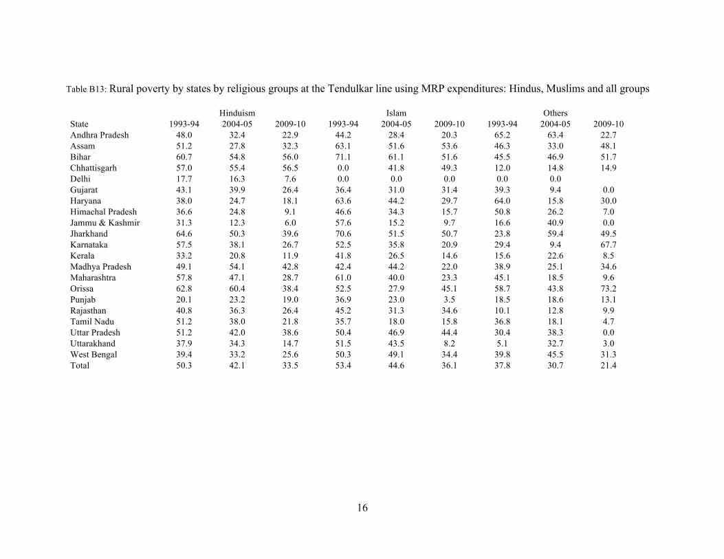
16

Table B13: Rural poverty by states by religious groups at the Tendulkar line using MRP expenditures: Hindus, Muslims and all groups

Hinduism

Islam

Others

State 1993-94 2004-05 2009-10 1993-94 2004-05 2009-10 1993-94 2004-05 2009-10 Andhra Pradesh 48.0 32.4 22.9 44.2 28.4 20.3 65.2 63.4 22.7 Assam 51.2 27.8 32.3 63.1 51.6 53.6 46.3 33.0 48.1 Bihar 60.7 54.8 56.0 71.1 61.1 51.6 45.5 46.9 51.7 Chhattisgarh 57.0 55.4 56.5 0.0 41.8 49.3 12.0 14.8 14.9 Delhi 17.7 16.3 7.6 0.0 0.0 0.0 0.0 0.0

Gujarat 43.1 39.9 26.4 36.4 31.0 31.4 39.3 9.4 0.0 Haryana 38.0 24.7 18.1 63.6 44.2 29.7 64.0 15.8 30.0 Himachal Pradesh 36.6 24.8 9.1 46.6 34.3 15.7 50.8 26.2 7.0 Jammu & Kashmir 31.3 12.3 6.0 57.6 15.2 9.7 16.6 40.9 0.0 Jharkhand 64.6 50.3 39.6 70.6 51.5 50.7 23.8 59.4 49.5 Karnataka 57.5 38.1 26.7 52.5 35.8 20.9 29.4 9.4 67.7 Kerala 33.2 20.8 11.9 41.8 26.5 14.6 15.6 22.6 8.5 Madhya Pradesh 49.1 54.1 42.8 42.4 44.2 22.0 38.9 25.1 34.6 Maharashtra 57.8 47.1 28.7 61.0 40.0 23.3 45.1 18.5 9.6 Orissa 62.8 60.4 38.4 52.5 27.9 45.1 58.7 43.8 73.2 Punjab 20.1 23.2 19.0 36.9 23.0 3.5 18.5 18.6 13.1 Rajasthan 40.8 36.3 26.4 45.2 31.3 34.6 10.1 12.8 9.9 Tamil Nadu 51.2 38.0 21.8 35.7 18.0 15.8 36.8 18.1 4.7 Uttar Pradesh 51.2 42.0 38.6 50.4 46.9 44.4 30.4 38.3 0.0 Uttarakhand 37.9 34.3 14.7 51.5 43.5 8.2 5.1 32.7 3.0 West Bengal 39.4 33.2 25.6 50.3 49.1 34.4 39.8 45.5 31.3 Total 50.3 42.1 33.5 53.4 44.6 36.1 37.8 30.7 21.4

17

Table B14: Urban poverty by states by religious groups at the Tendulkar line using MRP expenditures: Hindus, Muslims and all groups

Hinduism

Islam

Others

State 1993-94 2004-05 2009-10 1993-94 2004-05 2009-10 1993-94 2004-05 2009-10 Andhra Pradesh 33.8 22.1 16.0 44.5 32.7 24.7 19.4 11.6 3.2 Assam 25.2 21.5 21.4 50.4 24.2 52.7 0.0 22.7 13.1 Bihar 38.7 40.1 35.9 59.2 60.8 56.5 14.6 2.5 6.3 Chhattisgarh 30.4 28.1 25.2 16.7 54.4 10.4 5.6 4.4 3.0 Delhi 15.2 12.8 14.9 33.1 21.7 14.1 0.0 2.7 1.5 Gujarat 25.7 17.7 13.8 45.6 42.3 42.4 12.4 20.8 2.1 Haryana 23.3 22.5 22.2 51.7 46.5 42.4 38.5 0.4 20.0 Himachal Pradesh 13.7 5.2 11.7 0.0 1.7 51.4 20.7 0.0 0.0 Jammu and Kashmir 6.9 5.5 8.4 22.8 13.0 17.6 0.0 11.2 25.5 Jharkhand 40.4 21.7 30.6 55.0 49.8 44.3 18.5 29.5 9.8 Karnataka 30.7 23.0 19.9 50.6 40.3 20.4 13.1 2.2 6.5 Kerala 23.7 19.0 12.6 27.6 23.7 17.1 18.2 9.6 2.4 Madhya Pradesh 31.5 33.5 22.0 36.4 48.3 31.7 34.5 2.7 0.8 Maharashtra 27.5 20.1 15.2 44.0 47.9 30.9 14.5 12.0 10.2 Orissa 33.5 36.4 26.3 52.8 44.2 27.6 10.5 41.7 0.0 Punjab 27.5 20.5 17.3 50.8 40.5 23.7 23.7 20.9 7.6 Rajasthan 26.7 28.0 18.0 52.5 42.4 29.5 22.4 7.0 16.2 Tamil Nadu 33.3 20.1 12.6 35.4 19.1 11.2 29.6 29.3 4.3 Uttar Pradesh 33.4 27.5 24.7 50.7 48.4 49.5 23.1 32.3 8.5 Uttarakhand 18.5 24.2 17.1 32.5 44.3 49.4 0.0 0.0 26.1 West Bengal 27.3 20.9 20.0 56.1 45.7 34.9 20.6 22.1 15.9 Total 29.5 23.1 18.7 46.4 41.9 33.9 22.8 13.5 12.9

Program on Indian Economic Policies

Columbia University in the City of New York420 West 118th Street3rd Floor, Mail Code 3355New York, NY 10027Email: indianeconomy@columbia.eduindianeconomy.columbia.edu

September 2013