a comprehensive guide to agricultural …pdf.usaid.gov/pdf_docs/pnadl008.pdfa comprehensive guide to...

A COMPREHENSIVE GUIDE TO AGRICULTURAL LOAN PRODUCT DESIGN FOR UGANDA’S RURAL FINANCIAL

INTERMEDIARIES

The author’s views expressed in this publication do not necessarily reflect the views of the United States Agency for International Development or the United States Government.

Rural SPEEDA USAID funded projectContract No. PCE-1-00-99-00003-00, TO 826

TABLE OF CONTENTS

Review of Basic Financial Theory Underpinning Lending Operations 3

Demand Analysis and Qualified Demand Analysis 13

Selecting Bankable Enterprises 23

Analysis of Capacity to Supply a Loan Product 29

Initial Planning of Product Cash Flows 45

Risk Mitigation and the Affiliated Variable Costs 55

Loan Procedures and Costs 59

Product Costing and Interest Rate Determination 69

Product Promotional Strategy 87

Product Re-Evaluation 89

1

Chapter I

Review of Basic Financial Theory Underpinning Lending Operations

IntroductionProvision and recovery of credit is not a simple task. The lender will always face challenges of choosing the right borrower, financing the right business and recovering what has been loaned at a profit. This manual is meant to address the design of effective agricultural loan products. Agriculture is often the most difficult sector to lend to because the lender’s under-standing of the business is often limited and information for making lending decisions is often difficult to come by. The purpose of this manual is to equip the lender to raise critical ques-tions regarding an agricultural lending opportunity, research the answers to those questions and produce a product which is both profitable and sound from a lending risk perspective.

In order to effectively engage in lending for any business, certain theoretical issues surround-ing effective lending operations must first be understood. A basic theoretical grounding will enable the lender to first see if the logic behind their idea for a loan product is sound before digging in to the difficult tasks of designing the product. Core theoretical issues include:

6 A clear understanding of markets, supply and demand for credit;

6 A clear understanding of loan products with respect to their profit, risk and costs; and

6 A clear understanding of the need for a loan product to meet both the needs of the borrower and the lender at the same time.

Each of these topics will be handled in turn over the coming pages.

Markets, Supply and Demand for Credit:In simple terms, a market is a place where buyers and sellers of goods and services meet. Markets can be actual (a local market where traders come daily) or virtual (buying and selling goods and services over the telephone or internet). All goods and services have markets. There are markets for agricultural products, manufactured goods, labor, advice and, most importantly for the purposes of this manual, credit.

Given that a market is a place where buyers and sellers meet, a clear understanding of buyer and seller behavior becomes necessary before an understanding of the market itself is possible. This is where defining supply and demand becomes relevant. In markets there are two types of actors, producers and consumers. Producers supply goods and services; consumers demand goods and services. The behavior of each of them can be described as follows:

6 Producers supply a larger quantity of a good or service as the price for that good or service increases; producers supply a smaller quantity of a good or service as the price for that good or service decreases.

6 Consumers demand a smaller quantity of a good or service as the price for that good or service increases; consumers demand a larger quantity of a good or ser-vice as the price for that good or service decreases.

6 Like with all goods and services, credit also has a price. The price of credit is measured in terms of the interest rate the producer charges and the consumer

3

pays. The producer of credit in this case is the financial institution and the consumer in this case is the borrower. When interest rates are low the borrower will demand more credit; when interest rates are high the borrower will demand less credit. When interest rates are high the lender will supply more credit; when interest rates are low the lender will supply less credit.

6 In addition to price, buyers and sellers may also consider other issues when making trading decisions such as quality, location, cost of traveling to the market and packag-ing of the product.

At some point the demand from borrowers is equal to the supply from lenders. It is at this point that a market is created (borrowers and lenders are meeting and agreeing a quantity and price). This is called market equilibrium and this equilibrium will determine the amount of credit available to the borrowers and the interest rate at which that credit is available.

The ability of a financial institution to supply credit is decided by the institution’s costs. Because this manual is written for financial institutions, a greater understanding (and ex-planation) of supply is relevant. This is the topic of the next section.

Determining the Effective Supply of Credit:

The previous section provided a simple explanation of supply and demand. This section will expand that simple explanation by going into greater depth with respect to supply. Supply can be divided into simple supply and effective supply.

QUANTITY

PRIC

E

SUPPLY

QUANTITY

PRIC

E

DEMAND

QUANTITY

PRIC

E

DEMAND

SUPPLY

EQUILIBRIUM

5

Simple supply is determined by the cost of funds that a financial institution must pay to acquire its loanable funds. Normally, simple supply is determined by the interest rate the financial institution must pay to its depositors or its lenders (its cost of liabilities). In the il-lustration below, this supply is represented by S1.

Note carefully, that if we consider only the cost of loanable funds the equilibrium is very low on the demand curve. You can see that the equilibrium price of credit is low and the equilibrium quantity of credit supply is high. However, this is not reality because other than the cost of loanable funds, there are many other costs that a lender must account for in an interest rate.

Effective supply of credit considers not only the cost of loanable funds but also all other costs the lender must incur to make and recover a loan. These include the operational costs (staff costs, building costs, computer costs, vehicle costs, utilities, etc.), inflation costs (the fact that money loaned is losing purchasing power), the costs of expected losses from default and a profit margin to help the institution grow and pay its owners a dividend . If we consider these we come to the actual costs of lending and the effective supply of credit (now S2) as reflected in the illustration below.

Note carefully that when we see the real costs of lending, the effective supply of credit to the market changes remarkably compared to the simple supply. Also, the new equilibrium shows clearly that after considering the actual costs of lending, there is a smaller quantity of credit available at a higher price to the borrower. Understanding and accounting for the costs of lending is essential to designing an appropriate and functional agricultural loan product.

QUANTITY

PRIC

ES1

QUANTITY

PRIC

E

S1

DEMAND

QUANTITY

PRIC

E

S1

S2 Cos

ts o

f le

ndin

g

QUANTITY

PRIC

E

S1

S2 Cos

ts o

f le

ndin

g

DEMAND

Note that this new price is the supplier’s (lender’s) price. Borrowers may have to pay more in travel and bureaucracy to access and repay loans. Lenders should consider borrower costs of access to remain com-petitive in their own market.

7

Profit, Risk and Cost

The actual purpose of any loan product, agricultural or otherwise, is to maximize profit to the institution and to minimize risk2 to the institution. Both of these functions have a direct impact on the costs to the institution and therefore the effective interest rate at which credit is supplied.

Profit is itself the difference between revenue (what the institution earns) and cost (what the institution must pay to earn its revenue). Although the institution must maximize profit, this statement must be conditioned to include the fact that the market will only allow an institution to charge a reasonable rate of interest. If the interest rates are too high, as illustrated in the supply and demand review above, the quantity of credit demanded will be very low. There-fore, if the market will only allow interest rates to rise to a certain point, then the only way for an institution to maximize profit is to minimize costs of delivering and recovering credit. This manual is meant to help lenders to identify all of the costs of lending and to encourage the lender to be as efficient as possible in dealing with these costs because as the costs are minimized, more of the revenue is left over for profit.

Profit is important to a financial institution because it is from this profit that the institution can: increase its loan portfolio to service more and bigger clients, improve efficiencies by invest-ing in systems and technology, demonstrate to other businesses that the institution itself is a success and pay its investors (members in the case of a SACCO) good dividends which will help them to become more wealthy. The greatest threat to a financial institution is default and arrears. Loan default not only means that the institution loses its investment, it may also mean that the institution will be unable to pay back its depositors. Loan arrears, though less severe than default, can lead to problems with liquidity. If loans are not paid back on time, depositors funds may not be available when they claim them (undermining client confidence in the financial institution) and/or other borrowers will not receive their loans on time (which negatively impacts both the borrowers’ businesses and the perception of the institution in its market). Furthermore, inadequate liquidity as a result of default or arrears may have regulatory consequences such as suspending operations, or closing and liquidating the institution.

Risk cannot be eliminated, but it can be minimized. The very act of minimizing risk pro-duces a number of costs to the institution which must be reflected in the interest rate as will be explained later in this manual in the chapter covering Risk Mitigation. The real science behind a loan product is setting an interest rate which maximizes profit (by providing loans at an interest rate that attracts quality borrowers and minimizing the costs of lending), while minimizing risk (by covering the necessary risk management costs).

Excessively high interest rates (because costs are not controlled) encourage only those bor-rowers who can’t get credit anywhere else (the most likely borrowers to default) to borrow. This is not minimizing risk. Artificially low interest rates encourage large numbers of borrow-ers but leave the institution unable to monitor and recover the credit (because costs are not adequately planned for). This also is not minimizing risk.

2Principally risk includes the risks of non repayment (default) and/or late repayment (arrears).

9

Effective Product Design

The previous sections have covered the market for financial institutions where the price at which credit can be supplied and demanded is measured by the interest rate. Further cov-ered was the fact that effective supply of credit (and effective interest rates by implication) must take into account the full costs of lending (cost of loanable funds, operational costs, in-flation costs, reserves for losses and profit margin) which lowers the amount of credit avail-able and raises the price of that credit. Finally, the previous section covered the importance of maximizing profit and minimizing risk by first incurring sufficient costs to appraise and monitor borrowers but by secondly keeping those costs to a minimum to leave the maximum revenue for institutional profit.

All of these points are concluded in this section where effective product design will be dis-cussed. An effective loan product design, in the simplest terms, is a design which both satisfies the needs of the borrowers and the needs of the lenders at the same time. From the lender’s perspective, profit must be maximized and risk minimized while providing a product at an interest rate that a large number of borrowers can afford. From the borrower’s perspective the loan must be large enough to cover the business being borrowed for; the interest rate low enough for the borrower to be able to repay and remain with a reasonable profit on the business they are borrowing for; and, the timing of the loan must be ideal for the business being conducted. Both the borrower and the lender must be mindful of their capacities. The borrower must be capable of using the loan effectively to earn a profit on their business and repay the lender. The lender must be mindful of their capacity to understand the borrower’s business, ap-praise the borrower, monitor and recover the loan. The illustration below demonstrates the overlap of borrowers’ and lenders’ priorities:

Any product that meets the client’s needs without meeting the financial institution’s needs is not an appropriate loan product. Conversely, any product that meets the financial insti-tution’s needs without meeting the client’s needs is also not an appropriate loan product. Operationalizing this idea goes beyond simply understanding it. The financial institution’s policies and procedures must embody the appropriate product design, be made public and be well understood by both the borrower and the lender.

BORROWERS

Priorities Price Capacities Timing

LENDERS

Priorities Price Capacities Timing

APPROPRIATE

LOAN

PRODUCT

11

Chapter II

Demand Analysis and Qualified Demand AnalysisBackground

As was discussed in Chapter I credit markets are governed by effective supply of credit (that is the cost of funds plus the costs of delivering the credit). Beyond this there is what is called qualified demand. Agricultural loan products, like any other loan products, must be underpinned by existence of effective and sustainable demand. Qualified demand refers to what clients are willing to pay for whereas demand refers only to what clients want. Demand must be identified and qualified demand must be verified. The demand for a loan product must be backed up by a viable business from which the loan repayments will be made. This implies that the business must generate adequate positive margins to cover costs and ensure lender repayment and attractive returns to the borrower. If the realizable margins on the activity are negative or zero the risk of repayment default is very high. Obviously, if the realizable margins are positive the risk of default will be lower (though the risk of willful default must still be considered by the lender).

Both the capacity and willingness of the borrower to repay constitute core considerations in demand analysis. Capacity is characterized by adequate resources and cash flows on the part of the borrower. Willingness is less tangible and refers more to the borrower’s ethical personality, trustworthiness and attitude.

The total potential demand (critical mass) of borrowers is an equally crucial consideration. A small number or dozens of viable undertakings in a locality may not constitute adequate demand. This necessitates ascertaining both the output volumes and the profitable farm enterprises’ activities within the catchment area of the financial institution.

Understanding Value-addition Chains

Value chain refers to every transaction in the production and marketing of a commodity. For example in rice, the value chain would include the business of wholesaling inputs, the busi-ness of retailing inputs, the business of converting inputs into rice (through farm production), the business of transporting rice, the business of milling rice, and the business of market-ing the milled rice. For each business in the value chain there are cash flows where goods and services are purchased and sold. Likewise there is value addition at each business. Assessing value addition should involve ascertaining the costs of each activity that renders realization of proceeds, matching the revenue against the costs and ascertaining the profit (loss) at each transaction point. There is need to have standard reference such as output per acre or a kilogram of the sold commodity at that particular transaction point. That is to say, how much it takes to produce or procure or process that kilogram that is sold to realize revenue and thus profit. See the following upland rice example.

13

Upland Rice Value Chain Map

Based on Kabarole, Hoima and Kumi rice farmers. Commercial financing for millers and traders.

Category of transaction Value Per Acre (2MT

yield)

Value Per KG

Value Added (UGX/KG)

Internal Rate of Return

Months Annual Return on

Investment

1. Input Retail (farm delivered)Rice SeedTSP/MOP fertiliserUrea fertiliserSatuni/Rical herbicide

Total Cost of Inventory

(36,000.0)(21,000.0)(50,000.0)(44,000.0)

(151,000.0)

(18.0)(10.5)(25.0)(22.0)(75.0)

Input Price (151,000.0) (75.0) 0.00 0% 1 0%

2. ProductionPloughing ServicesPurchased InputsHired Labor (field operations)Hired Labor (harvesting & handling)Packing

Total Costs of Production Before Financ-ing

(90,000.0)(151,000.0)(88,000.0)

(140,000.0)(14,000.0)

(483,000.0)

(45.0)(75.5)(44.0)(70.0)(7.0)

(241.5)

Farmgate paddy price 1,000,000.0 500.0 258.50 107% 8 161%

3. Milling/processing (Kampala-based mills)Paddy costTransport (local)HandlingMilling Loss (35% on above costs)Milling costs (power, depreciation, etc)Rent and overheadsTrade Finance (Total costs, 1.83%/month)

Total mill price, Transport, Handling & Storage

(1,000,000.0)(60,000.0)(6,000.0)

(373,100.0)(140,000.0)(76,363.6)(47,011.5)

(1,702,475.1)

(500.0)(30.0)(3.0)

(186.6)(70.0)(38.2)(23.5)

(851.2)

Millgate price 2,000,000.0 1,000.0 148.76 17% 1 210%

4. Wholesale Traders (Kampala-based Traders)Mill priceTransportHandlingRent and overheadsTrade Finance (Total costs, 1.83%/month)

Total mill price, Transport, Handling & Storage

(2,000,000.0)(20,000.0)(4,000.0)

(15,000.0)(37,374.9)

(2,076,374.9)

(1,000.0)(10.0)(2.0)(7.5)

(18.7)(1,083.2)

Price to Retail Shop (Kampala) 2,400,000.0 1,200.0 161.81 16% 1 187%

As is clear in the value chain map above, availability of reliable data is very important. Very often in agriculture, farmers and even rural traders, do not keep records on production and transaction costs, though they have fair knowledge of their revenues. Also, they do not properly cost some of the activities such as the use of family labor or acquisition costs for productive assets, and thus limit the accuracy and relevancy of the cost data. However, for financing purposes, the value chain analysis process can ignore some of these costs as sunk costs.

15

Value Chain Mapping is a powerful tool to determine whether or not an agricultural enter-prise will be creditworthy. Mapping value chains is a skill which should be developed by lenders in this market. This method helps the lender to verify:

1. Producers’ experience/knowledge;

2 Producers’ skills; and

3. Producers’ attitude towards commercialization.

The following are the necessary steps to follow to realize the mapping of a value chain.

Steps

1. Identify the sector for which demand analysis is to be done (for example rice pro-duction and marketing).

2. Select sample space from whom to gather data in an area. There is need to have a cross-cutting sample that includes best, average and poor performers.

3. Ascertain the costs of undertaking the agricultural activity that encompasses best practice say on an acre basis or metric ton basis. Take care to include all the trans-actions that are necessary to accomplish the activity and assign realistic costs to these activities, including the non-paid for activities.

4. Ascertain the fair profit margin for the transaction point. Make a judgment as to whether the margin is attractive enough to warrant borrowing over the transaction time. It is the level of the anticipated profit margin that is the major motivator for accessing credit for the transaction.

5. Ascertain the fair estimate of the number of actors for the transaction point and the commercial expertise for the activity in the geographical area.

6. Ascertain the availability of and accessibility to the productive resources that are critical for the successful accomplishment of the activities, including inputs, labor, equipment and facilities like storage and transportation.

7. Ascertain the availability, proximity and accessibility of external productivity and profitability enhancement opportunities such as extension services and technical assistance.

Internal Rate of Return (IRR)

For an activity to qualify for borrowing presupposes that the activity must generate a positive financial return and is thus capable of realizing revenue that surpasses its costs, including financing costs. All entrepreneurs undertake activities in anticipation of realizing profit, and the higher the expected rate of return, the bigger the motivation to successfully undertake the activity. Basically any loan product must ensure that the venture to be financed has the capacity to generate what is called a positive Internal Rate of Return. Internal Rate of Return refers to the percentage financial return of a given business excluding all cash flows external to the business.

The rate of return for agricultural activities may not necessarily need to be based on comple-tion of the agricultural cycle but rather analyze each business along the value chain inde-pendently. Thus an internal rate of return may be ascertained for the farm-level activities, rural trading and regional trading activities as opposed to looking at all of these at once. It is prudent for product development to ascertain the internal rates of return for the various transaction points in the commodity value chain and thus tailor any product development to

17

particular segments of the chain that are highly profitable and with less risk. Analysis of the entire value chain also helps to understand the commercial synergies within the chain. For instance financing for an otherwise attractive field level rate of return can be thwarted by a low or negative return realizable at the marketing transaction point and vice versa.

Calculating Simple IRR

In simplest terms IRR can be defined as follows:

IRR = [(Total Revenue per KG – Total Cost per KG) ÷ Total Cost per KG] x 100%.

This figure tells us how much the business can pay in interest before it starts to make losses.

For example, from the value chain map presented earlier, in rice production we have a to-tal cost per acre of UGX 483,000 (including land, labor, inputs, etc.), total revenue of UGX 1,000,000 and a total output of 2,000 KG per acre. To calculate the IRR, you first work out the cost per KG which is UGX 242 and the revenue per KG which is UGX 500. You then subtract the total cost from the total revenue, divide that result by the total cost and then multiply that figure by 100% resulting in 107%. This result tells the lender that a potential borrower can pay up to 107% interest on the total costs of the business before they begin to earn losses. This should be very encouraging to a lender.


yield)

Value Per KG




Investment



(90,000.0)(151,000.0)(88,000.0)

(140,000.0)(14,000.0)

(483,000.0)

(45.0)(75.5)(44.0)(70.0)(7.0)

(241.5)


It is often important to express the IRR in both transaction period and annual rates to facili-tate easy comparison of financing costs and the expected return. In the example above, financing an agricultural business whose rate of return for eight months is 107% percent (results in an annual IRR of only 161%) with a loan bearing interest and charges of 4% per month the borrower will certainly have the capacity to repay.

It is wise for the lender to also look at the sensitivity of the loan to price changes for the farm gate price. What happens, for example, if the price drops to UGX 400 per KG?

19


yield)

Value Per KG

Value Added

(UGX/KG)



Investment


Total Costs of Production Before Financing

(90,000.0)(151,000.0)(88,000.0)

(140,000.0)(14,000.0)

(483,000.0)

(45.0)(75.5)(44.0)(70.0)(7.0)

(241.5)

Farmgate paddy price 800,000.0 400.0 158.50 66% 8 98%

We can see from the example above, that the borrower still earns 66% for the business and could therefore still be capable of paying 4%/month for the loan. What happens if the price drops to UGX 300 per KG?


yield)

Value Per KG

Value Added

(UGX/KG)



Investment



(90,000.0)(151,000.0)(88,000.0)

(140,000.0)(14,000.0)

(483,000.0)

(45.0)(75.5)(44.0)(70.0)(7.0)

(241.5)

Farmgate paddy price 600,000.0 300.0 58.50 24% 8 36%

Here we see that the borrower now earns only 24% for the business and therefore could not pay 4% per month. The lender should be keenly aware of what the history of price changes has been for a given commodity to make a good judgment regarding how susceptible this loan is to price risk.

21

Chapter III

Selecting Bankable EnterprisesAs earlier presented, it is imperative to finance a bankable enterprise, bankable in the sense that the enterprise is capable of generating positive IRR and thus able to repay the loan prin-cipal and interest and fees, while generating surplus for the entrepreneur as a motivation for further engagement in the same activity. Agricultural enterprises with annualized IRR that are significantly higher than interest and lending charges ought to be bankable.

IRR alone constitutes a necessary condition for enterprise selection but is not by itself suf-ficient. There are other considerations that constitute sufficient conditions for enterprise selection. These include: the duration within which the business cycle will be completed; the regularity of the business cash flow; the volume of the business within the geographical area; the attributes of the entrepreneurs, including their experience, skills and attitude; the availability of and accessibility to production resources such as inputs, labor, tractors, stor-age, transport, quality enhancing equipment, etc; access to stable and sustainable market; and existence of external support such as field extension services and technical assistance. These have direct impact on both the capacity and willingness of the borrowers to repay and on the cost of delivering the credit by the financial institution.

Enterprises with short completion cycle and regular cash flows have lower risk of loan default compared to those with longer terms and irregular cash flows. Also existence of productivity enhancing inputs and resources, and access to external support reduce the risk of potential loan default by increasing the IRR through reduced unit cost of production. The existence of a critical volume of business in the geographical area can help to substantially lower loan delivery and recovery costs and thus increase profit realized on loans or provide leverage for lower lending charges. Finally the existence of a stable market for the commodity provides a sound base for realization of sustainable positive IRR. Commodities with fluctuating market prices and marketable volumes present higher risk for financing as the lending institution is bound to face loan recovery difficulties during overproduction, commodity market slumps and price collapses. Conversely, commodities with stable and assured markets such as forward contracted production present lower risk for lenders.

Ranking Potential Investments

It is important to rank the potential bankable investments (enterprises) and thus select those that have a lower potential for non repayment before designing a loan product. A fair criteria needs to be developed to guide a realistic and quantitative investment ranking process. The following variables, in order of priority, are suggested for ranking agricultural enterprises for which appropriate loan products can be designed for financing purposes:

6 Positive Internal Rate of Return

6 Existence and stability of the market

6 Tenure of the activity to be financed

6 Timing of its cash inflows

6 Level of commercialization or volume of business in the given location

6 Availability of production resources

6 Accessibility to external technical support

23

See the example of Ranking Criteria Table below:

IRR Market Strength Tenure (months) Timing of Income

Analysis Score Analysis Score Analysis Score Analysis Score

< 20 % 1 Poor 0 > 12 1 At harvest > 1 year 1

20 – 30 % 2 Fair 1 8 – 12 2 At harvest > 6-12 months 3

30 – 40 % 3 Good 2 4 – 8 5 At harvest < 6 months 7

40 – 50 % 5 V/Good 4 3 – 4 7 Regular 10

> 50 % 10 Excellent 10 < 3 10

Level of Regional Commercialization

Availability of Production Resources

Access to Technical Support

Analysis Score Analysis Score Analysis Score

Poor 1 Poor 0 Poor 1

Fair 2 Fair 1 Fair 2

Good 5 Good 3 Good 3

V/Good 7 V/Good 7 V/Good 6

Excellent 10 Excellent 10 Excellent 10

Scoring Potential Enterprises

Use the table below, or one similar, to score the potential enterprises and rank them. Tables such as this really assist a financial institution in making scientific determinations of the best potential loan products. There is a filled in example at the end of this section.

Attribute Enterprise 1 Enterprise 2 Enterprise 3


IRR (annual)

Market stability

Tenure

Regularity of cash flows

Volume of business

Access to resources

Access to external support

Overal Score

Overall Score In order for the FI to diversify risk, realize portfolio balance and minimize operational loan-related costs, it may be prudent for it to select more than one agricultural enterprise in a geographical location for which separate loan products can be developed. For instance if rice and maize production in an area can meet the desired ranking criteria scores, it may be appropriate to design loan products for the two commodities in order to minimize loan delivery operational costs and maximize loan revenue.

25

A fundamental question arises here as to whether selection of bankable enterprises should be done internally by the financial institution staff or through external sourcing. There is no cut-off point on this. If the institution has adequate capacity to undertake this activity, it may serve better as it provides better understanding of the sector for subsequent lending deci-sions once the product has been designed. However, if the internal capacity is inadequate or there is a critical staff time constraint, external expertise may suffice. Though in the latter case it may be very important to attach a staff to the externally sourced personnel to gain a deeper insight on how the activity is accomplished and minimize potential for future misun-derstanding in regard to the enterprise selected.

Comparison of Commodities for Financing (Rice, Maize and Sun Flower - Production)

Attribute Maize Rice Sunflower


IRR (annual) 36% 3 107% 10 42% 5

Market stability Very Good 4 Very Good 4 Excellent 10

Tenure (months) 8 2 8 2 4 5

Regularity of cashflows

At harvest6-12 months

3 At harvest6-12 months

3 At harvest < 6months

7

Volume of business Very Good 7 Good 5 Very Good 7

Access to resources Very Good 7 Fair 1 Poor 0

Access to external support Good 3 Very Good 6 Very Good 6

Total Score (Max 70) 29 31 40

Source: USAID Rural SPEED commodity value chain analysis reports.

From the above ranking, the financial institution is able to select an enterprise or enterprises for which to develop one or more loan products. In the above case sunflower production would provide the best option, followed by rice and maize. However, it must be reiterated that the enterprise IRR as measured against the financial institution’s lending rate, should have a critical bearing on the selection of the enterprise to fund.

This analysis is practical even if there is only one enterprise to rank as it still provides a criti-cal lens through which to evaluate the lending opportunity. In this case the Board of Direc-tors of the financial institution should set a minimum score below which the loan product will not be developed.

27

Chapter IV

Analysis of Capacity to Supply a Loan ProductIn the previous chapter, this manual addressed identifying loan opportunities. This chapter is dedicated to self evaluation of the financial institution to verify that it is capable of effec-tively supplying the credit. Toward that goal, this chapter will provide guidelines to financial institutions to analyze their ability to cost effectively generate loanable funds; review the financial institution’s internal staff capacities to appraise, lend and recover; review the fi-nancial institution’s physical resources for effective loan management; consider competition with both other financial institutions and with other products being offered by the financial institution itself; and finally to consider the needs of balancing lending for agriculture with lending for other, less risky, opportunities.

Availability of Offsetting Liabilities, Their Terms and Conditions:

Obviously, the most critical element in offering a loan product is having the funds available for lending. No client wishes to come to a financial institution, apply for a loan, and endure the approval process only to learn that the institution doesn’t have the money to lend.

In accounting terms, loans occupy the Asset side of the balance sheet because they are obligations owed to the financial institution just like debts owed to a business. These assets are obligations on the part of the borrower to pay the financial institution both the principal borrowed, the interest due for the costs of delivering the loan and for the privilege of access-ing the loan. It is also clear in accounting terms that without the Liabilities and Equity side of the balance sheet, providing any loan (to become an Asset) is impossible. In other words, assets must be backed by funding resources.

Liabilities are normally made up of various types of savings deposits and loans to the finan-cial institution from wholesale lenders. These are obligations the institution must repay at a specified time in the future. It is normally Liabilities that provide the majority of a financial institution’s loanable funds. In relation to loan Assets, Liabilities are often referred to as Offsetting Liabilities. This is because the obligation of the borrower to pay the loan (an As-set to the financial institution) is offset by an obligation of the financial institution to repay a depositor or lender (a Liability).

Equity, the remaining balance sheet category, is normally made up of owners’ shares (mem-bers’ shares in the case of a SACCO), any grants the institution may have received and retained profits. Equity is considered more stable than Liabilities as owners’ shares are only paid out when the institution is closed and retained profits are considered the property of the institution itself. However, Equity is normally inadequate for funding loans and is usually used as reserve funds within the financial institution. Thus, in order to make loans, Offset-ting Liabilities are, by and large, the most important funding source.

The fact that Offsetting Liabilities are the most important source of loanable funds forces a financial institution to consider and manage some key issues. These include:

6 Value of Offsetting Liabilities;

6 Timing of Offsetting Liabilities; and

6 Cost of Offsetting Liabilities.29

Value of Offsetting Liabilities

In terms of value of Offsetting Liabilities, a financial institution should pursue having at least the same value of Offsetting Liabilities as it has in loans. This is the essence of financial intermediation. That is, bring in liabilities at a low interest rate, consolidate these liabilities and lend them out at a high interest rate. By using, to the greatest degree possible, Liabili-ties to finance the loan portfolio, the institution reduces the risk to its Equity which is the key to long term sustainability.

Timing of Offsetting Liabilities

One problem that arises with using Offsetting Liabilities to finance the loan portfolio is the need to manage the timing of Offsetting Liabilities. Obviously, when a financial institution borrows for on lending, the loan must be repaid. If the loans to the institution come due before the loans from the institution to its clients come due, the institution risks illiquidity or worse, insolvency. This is also true for other liabilities such as savers’ deposits.

Using voluntary deposits as Offsetting Liabilities is extremely risky because these deposits can be demanded by depositors at any time. In order to mitigate this risk, the institution must always keep adequate cash on hand to meet voluntary withdrawals. To adequately plan for this, the institution must monitor on a regular basis client demands for their volun-tary deposits3. When the institution is sure that they have more than adequate liquidity at all times to meet client withdrawals, the balance of these demand deposits can be used as Offsetting Liabilities to finance loans.

Using fixed deposits as Offsetting Liabilities is perhaps the best way to finance lending. With a fixed deposit, the financial institution guarantees the depositor an increased return on their deposit because the depositor guarantees the financial institution that they will not withdraw the fixed deposit before it matures. Normally, a financial institution will determine its loan opportunities, the time when loans will be repaid and then offer its clients fixed de-posits in the same value of the total loan opportunities to mature after the loans are repaid. This is a very stable method of financing the loan portfolio and has the added advantage of building clients’ propensity to save.

It is critical to note that the timing of Offsetting Liabilities must be managed. Default and/or arrears in the lending operation will lead to delays in paying back wholesale lenders and de-positors. These delays erode confidence in the institution and in the worst case can lead to insolvency. The structure of Offsetting Liabilities has a bigger impact on setting loan product terms such as grace periods, loan duration and both timing and size of loan installments. Very often there is a concerted debate in favor of longer term loans and grace period for agricultural loans to match the gestation periods of the agricultural ventures. Such ideas are only feasible if the maturity of the existing Offsetting Liabilities allow for them.

3 Often, for example, the weeks preceding Christmas holidays and school opening calendar are times when many demand deposits are withdrawn.

31

Cost of Offsetting Liabilities

The last point to consider regarding Offsetting Liabilities is the issue of their cost. This cost is normally the interest the financial institution must pay to the lender or depositor for the use of these funds plus the operational cost to the institution to manage these funds. The three methods of generating Offsetting Liabilities mentioned above have different cost im-plications for the institution. While voluntary deposits are the least costly source of funds in terms of interest payable, they are also the least predictable and therefore the most costly to manage. Fixed deposits normally fall next in terms of interest payable and require rela-tively less management once they are secured. The problem, of course, with fixed deposits is that savers may not have enough money to invest in fixed deposits or they may not have the ability to wait the allotted time to be repaid with interest. Borrowing funds from a whole-sale lender is usually the highest cost solution for generating Offsetting Liabilities. Interest payable on wholesale loans is normally higher than interest payable on voluntary or fixed deposits. The cost of acquiring the funds can also be considerable if it entails multiple visits and bureaucratic procedures with a large lender. Finally, management time can also be considerable depending on the repayment terms.

Finally, it may not be prudent to use a single source for a financial institution’s Offsetting Liabilities. Voluntary deposits are somewhat unpredictable; fixed deposits are somewhat difficult to come by; and, loans are expensive. It is perhaps best to balance the use of all three of these Offsetting Liabilities while paying close attention to the value needs, the tim-ing of repayment and the costs of using them.

Human Resource Capacity Assessment

Risk management, analysis and mitigation are critical in lending. Thus the need for effec-tive project appraisal, appropriate loan decisions, effective monitoring and loan recovery constitutes essential ingredients for an effective financial product portfolio, including agri-cultural products. Unfortunately not all the skills can perfectly cut across all loan products in lending situations. Agricultural lending, especially for production, requires unique skills different from strict commercial lending. Lending for agriculture, to enhance realization of a higher IRR, requires careful appraisal (both technical and analytical) of the business and of the borrower; timely lending decisions; appropriate loan amounts; appropriate disburse-ments; proper business monitoring and understanding the external factors such as climatic and market trends.

Any financial institution interested in developing and offering an agricultural loan product must evaluate the capacity of its human resources that will design and deliver the product. Stringent agricultural lending processes call for appropriate skills within the financial insti-tution contemplating introducing agricultural lending. This doesn’t necessarily mean that the institution must possess the staff with appropriate skills but there must be deliberate and realistic plans to have such staff to implement the loan product. It may further not be necessary for a financial institution contemplating introducing agricultural lending to have or recruit graduates of agricultural disciplines. As mentioned earlier, feasibility analysis and product design skills can be externally sourced if the institution lacks such skills. However, the human resource, with appropriate skills, to deliver the product must be internal within the institution.

The financial institution can enhance its skills through selectively recruiting staff that have formal agricultural training background or those that have accessed informal training in agricultural lending, including field coaching. Also a deliberate skills enhancement program can improve skills for agricultural lending among the existing staff of the financial institution,

33

especially in collaboration with entities promoting agricultural production, financing and mar-keting programs. Such entities include donor projects, NGOs and government agencies.

Other important attributes for human resource capacity assessment include adequate num-ber of agricultural loan officers, attitude of the loan officers towards handling agricultural credit and motivation of the loan officers in the agricultural portfolio. The loan-load for agri-cultural loan officers directly affects the timing of the loan decisions. Very often agricultural businesses in a given geographical location have peak timing and thus exert pressure on loan officers. Unlike commercial business, any delay in financing decisions for the agricul-tural business directly impacts the borrower performance and loan repayment capacity. It is therefore crucial that either the financial institution has adequate number of loan officers to appraise the applicants or the appraisal and loan decision process be scheduled much ahead of the peak period (though disbursement will coincide with the activity timing).

Most often loan officers in financial institutions tend to prefer handling non-agricultural cli-ents and if possible would want to entirely avoid agricultural clients in their loan load. It may thus be preferable to have loan officers dedicated purely to the agricultural portfolio and this may be appropriately specified at the time of recruitment. Much of the negative inclination to agricultural clients is associated with personal attitude of the loan officers and has no practi-cal relevance to career development or non-performance risk for the loan officers. It is thus a perception problem that clearly needs to be demystified.

Associated with the above is the need to institute a proactive agricultural portfolio incentive scheme within the financial institution. In a number of instances, agricultural loan officers encounter circumstances beyond their control that may impact their financial incentives, especially where the financial institution’s incentive system is based on standardized pa-rameters such as repayment according to a predetermined schedule. Such circumstances may include delayed rains and or bumper harvest that may delay marketing of the commod-ity. These may delay recovery of the loans and thus create artificial arrears that may lead to poor performance rating of the affected staff and consequent incentive penalties which cannot be reversed once the loans have been repaid after marketing of the commodity. Also the agricultural loan officers are subjected to many occupational field inconveniences and hazards such as rain, storms, exposure to airborne diseases, traveling long distances for appraisal and monitoring, and often on very poor rural roads. Thus there is need for a mo-tivational incentive scheme specifically tailored for the agricultural loan portfolio within the financial institution that addresses the unavoidable circumstances and also compensates for the personal field inconveniences.

Physical Resources for Effective Outreach and Portfolio Quality Main-tenanceJust as there is need for adequate and skilled human resources to deliver effective agri-cultural credit, the availability of and accessibility to appropriate physical resources within the financial institution is equally important. Agricultural staff must be mobile for effective appraisal, monitoring and loan recovery, and should be facilitated to explore future lending opportunities. Also there is need to have regular reliable information about the client and portfolio performance, in addition to ensuring regular contact with the borrowers and other collaborating partners.

The above warrants the institution to possess sound and appropriate transport facilities such as motorcycles, or, at least, bicycles and field-related accessories such as gum boots and rain coats, an effective Management Information System (MIS) for portfolio information processing and report production in addition to functioning communication facilities. The

35

transport equipment must be relevant to the terrain and road infrastructure of the geographi-cal area to ensure cost-effective, easy and timely outreach. In order to rationalize the fleet-related costs it is imperative that the loan officers develop cost-saving field schedules that facilitate serving many clients on each field visit. Functioning communication facilities such as mobile telephones can substantially leverage transport costs and provide easy means of maintaining regular contact with the borrowers.

The financial institution’s computer equipment should have appropriate software that facili-tates realistic appraisal analysis and effective performance monitoring, and ensure genera-tion of timely reports that reflect the quality of the portfolio. If the financial situation allows, the institution should ensure the availability of computer equipment purely dedicate to the agricultural portfolio.

In many instances, agricultural loan officers fail or delay to appraise and monitor their clients due to unavailability of transport, either physical transport or supplies such as fuel, and in some cases due to breakdown of the transport equipment in the field due to poor mainte-nance. Similarly, lack of computer equipment may impair the capacity of the loan officer to adequately track the loans in arrears that may lead to deterioration of the portfolio quality.

Competition and Borrower Behavior

Provision of financial services (in this case agricultural loan products) involves, among other things, competition. Competition in this respect involves two dimensions. On the one hand, there is competition with other financial institutions offering similar agricultural loan products and on the other there is the competition within the financial institution among loan products with regard to resource allocation and portfolio targets. The latter competition aspect can be effectively internally managed through clear profit center analysis and appropriate policies with emphasis on the capacity of the loan product to positively contribute to the profitability and goals of the financial institution. Of course there may be other secondary consider-ations that make the product internally competitive such as compatibility with the national policies such as the Plan for Modernization of Agriculture (PMA) and community support for the products. The perception among the institution’s policy makers and management of the risk of the loan product to be introduced will substantially influence its internal competitive-ness.

The external competition with institutions having similar product offerings ought to be of crucial consideration. If the quality and terms of the product offered by the competitors are better than what the institution can offer, it means the institution’s capacity to generate viable business with that product is undermined. Thus the institution contemplating introducing an agricultural loan product that is being offered by competitors must carefully evaluate its competitive advantage in offering the product and evolve mechanisms to consistently guard that competitive advantage. Competition among institutions offering the same or similar products will be determined by each institution’s policies and procedures.

Often financial institutions consider the cost of lending, and thus loan pricing, as the sole competitive variable, and also the sole concern for the borrower. However, it is evident from practice that cost of borrowing is often least considered by the borrowers. Similar to finan-cial institutions, borrowers want to maximize profit on the undertaking for which they borrow. They know what to do and what it takes to achieve it. Non-loan costs, such as convenience of access and timing of agricultural credit, as well as having a good credit relationship that builds sustainable trust between the client and the lender are major considerations for bor-rowers, beyond good loan pricing. For instance it is not worthwhile getting a low-priced agricultural loan which is disbursed two weeks late into the season versus getting a loan two

37

weeks ahead of the start of the season. Furthermore, borrowers prefer having the flexibility to reschedule their repayments to allow for successful marketing of the commodity versus getting an agricultural loan where their collateral may be disposed of when the marketing season is delayed despite the realization of good harvest.

Therefore, there is need for adequate competitor analysis and clear understanding of the behavior of borrowers in order to develop a loan product that will be relevant to the borrow-ers. This may require intelligence gathering that will involve obtaining information on com-petitors’ loan product policies and procedures and thus tailoring the institution’s loan product policies and procedures to harness a competitive position and sustainable market share. For example loan product policies and procedures that minimize non-direct loan access costs such as transport and time for the borrower, including in-the-field borrower screening and appraisal, can substantially increase the competitiveness of the institution’s agricultural loan product.

Another consideration for agricultural loan product competitiveness is the provision for regu-lar review of the product. Regular review allows for adjustment of product cost and price, and also the revision of the product delivery policies and procedures to match both the competition and the demand. The frequency of the product review should take into consid-eration the costs involved and the effect on the perceptions of the existing product clients. Any adjustments following a product review need to be beneficial to both new and existing clientele if the product is to remain competitive.

Portfolio Balancing Between Agriculture and Other Lending Activi-ties

One significant issue a financial institution must always consider is risk diversification. That is, a financial institution should never concentrate on a single strategy to generate either li-abilities or assets. On the Liability side, by offering different savings products and pursuing wholesale loans allow the institution to diversify not only its sources of funding but also the risk that comes with each of those sources. The same can be said on the Asset side. By offering different loan products targeting different types of businesses and investments, the institution can diversify not only its sources of income but also the risk that comes with each of those sources.

Agriculture, and particularly production, is a relatively risky sector. When a lender compares lending to a farmer to grow a crop the risks are much larger than lending to other ventures. Consider the table below comparing an agricultural production loan to a trade loan:

39

Consideration Agriculture Loan Trade Loan Discussion

Loan TermLonger (repayment after harvest and marketing)

Shorter (repayment aftergoods sold)

The longer a lender has its money in the borrowers’ hands the greater the risk the lender won’t be repaid.

Frequency ofRepayment Infrequent Frequent

Traders have daily cash flow which can be used to repay a loan, agricultural producers have a one time cash flow.Frequent repayment leads to frequent contact between borrower and lender; frequent contact means stronger relationships and less risk.

Borrower Location Far from Lender Close to Lender

Closer borrowers will have more interaction with the lender and a greater propensity to pay and pay on time. This is clearly less risky.

Tangible Collateral

Inputs which are purchased with the loan and expended during the production cycle.

Inventory purchasedwith the loan and resoldfor cash

Inventory is finished goods with a market value and can be seized or resold from a defaulting borrower; inputs are buried in the soil. Inventory is less risky.

Price Risk and Product Turnover

Farmers speculate onprice far at planting andfar in advance of harvest; they turnover their product only once.

Traders speculate on price in the near term and turn over their inventory frequently; if something doesn’t sell for a profit, they don’t stock it.

It is easier to predict the market price of a product one day in advance versus six or eight months in advance. Borrowers for trade are far less risky as a result.

WeatherFarmers rely on and hope for good weather.

Traders are largely unaffected by weather.

Weather can’t be predicted or controlled. Loans relying on good weather are more risky than those that don’t.

Clearly, relative to trade loans, agricultural loans are much riskier. However, just because something is riskier than something else, a lender cannot always avoid it. In order to grow the loan portfolio, a lender must lend to the opportunities in the geographical area. If a lender is in a rural area, the lender must consider agriculture. While the risks are consider-able, good loan management can mitigate most of the potential pitfalls. Remember that though agriculture is considered risky by lenders, every one of us still eats and the food we eat comes from farmers. The lesson is to be aware of the risks and to plan strategies to mitigate those risks versus simply avoiding the risks. Portfolio balancing is one strategy to mitigate risks.

Portfolio balancing in short means lending for a several well understood activities (for ex-ample dividing the portfolio among small trade loans, large trade loans, school fees loans, salary loans, agriculture loans, etc.). If one activity encounters problems, then the lender remains with other activities which should be immune to the same problem.

In the United States, conventional wisdom for rural banks is never to invest greater than 20% of the total loan portfolio in agricultural production. American rural lenders normally balance this with trade loans, small business investment loans and housing finance. Given that the US is a relatively highly developed agricultural society (with well functioning mar-kets, weather and price insurance, farmers with assets, widespread irrigation, etc.), it is

41

probably soundly logical if Uganda’s lenders also avoid investing greater than 20% of their total portfolio in production agriculture and balance that investment with 80% investments in less risky activities.

As a final point, it is worth noting that diversifying risk should also be addressed within the agricultural portfolio itself. It is wise for a financial institution to lend for several types of agricultural ventures so as to diversify the risks associated with each one. For example, by lending for both bananas and maize, if the banana crop is destroyed by wilt or another disease, there remains a high probability that the maize loans will continue to perform. The further advantage is that the lender maintains a continuous presence in its target market.

43

Chapter V

Initial Planning of Product Cash Flows:

Background

Cash flows, for accounting purposes can be divided into two basic types in a financial in-stitution. These are Operational Cash Flows and Financial Cash Flows. The Financial Cash Flows refer essentially to inflows and outflows of cash connected directly to saving, borrowing, lending and recovering (i.e. interest and principal). Operational Cash Flows, on the other hand, refers to income and expense on things such as fee income, monitoring ex-penses, office overhead, etc. The key elements to understanding cash flows (in either case) are to understand the timing element and the volume element of the cash flows.

It is not enough to say the institution will earn a certain income or pay a certain expense without specifying when and how much of these cash flows are expected. This is obviously critical in planning the institution’s liquidity so that the institution has neither too much money at a given time that is not earning income or too little money at a given time which forces the institution to borrow to meet short term needs.

Financial Cash Flows and Timing

As stated above, Financial Cash Flows refer to inflows and outflows of cash related directly to saving (deposits and withdrawals), institutional borrowing (borrowing and repaying) and lending (lending and recovering). All of these cash flows related directly to activities re-sulting in interest earned and/or paid. It is critical that adequate funds be available before promising:

6 Savers available cash when they want to withdraw savings, or

6 Creditors available cash when they are promised a loan repayment, or

6 Borrowers available cash when they are promised a loan disbursement

Without planning for these, the institution can be forced to borrow short term (at high interest and high expense for organizing the short term loan) to meet these obligations. Further, if the institution fails to find the short-term finance to meet these obligations, it will risk insol-vency and loss of client confidence.

Planning adequately for Financial Cash Flows begins at the product design phase. It is useless to offer a product without analyzing the impact that the product will have on the institution’s ability to meet its financial obligations with respect to volume and timing of cash available.

Operational Cash Flows and Timing

Again, as stated above, Operational Cash Flows refer to inflows and outflows of cash (in-come and expense) related to activities, which are not directly related to interest earned and/or paid. Operational Income is sourced from fees, sales of passbooks, commissions,

45

etc. Operational Expense covers things such as overheads, staff costs, transport, etc. As with Financial Cash Flows, it is critical that adequate funds be available to meet:

6 Staff salary payments

6 Loan monitoring costs

6 Payments to utility and service providers.

Again, without planning for adequate liquidity to meet these obligations, when they come due, the institution will lose the confidence of its employees, clients and creditors. Further, by not meeting the costs of loan monitoring, the institution again, puts its Financial Cash Flows at risk, which results in damaging the quality of the loan portfolio.

As with Financial Cash Flows, Operational Cash Flows also must be planned for in the de-sign phase of any product the institution offers. It makes no sense to offer a product only to realize that there is not adequate income at the right times to cover the costs, at the right times, of delivering and monitoring that product.

Upland Rice Example

When planning a new loan product, an essential exercise is to map the anticipated cash flows to determine the capacity of the institution to effectively deliver the product. The simplest way to do this is to draw a cash flow diagram. Before showing the Upland Rice Example, a general cash flow diagram will be explained.

Cash flow diagrams represent both the timing and volume of both inflows and outflows. This is normally represented by drawing an x-axis for time and various y-axes for volume. Posi-tive cash flows (meaning inflows to the institution) are above the x-axis and negative cash flows (meaning outflows from the institution) are below the x-axis.

-50

Jan Feb Mar Apr

+25 +25 +25

The above illustration shows the viewer that there is an anticipated outflow of 50 in Janu-ary and anticipated inflows of 25 in February, March and April. Modeling loan products in this way will help the institution to quickly determine if the timing and volumes of cash flows will meet their liquidity management needs. It is important to realize the true power of this diagram method. Multiple cash flow diagrams can actually be added together so that the institution can see the cash flow pattern of all of its products and activities together.

47

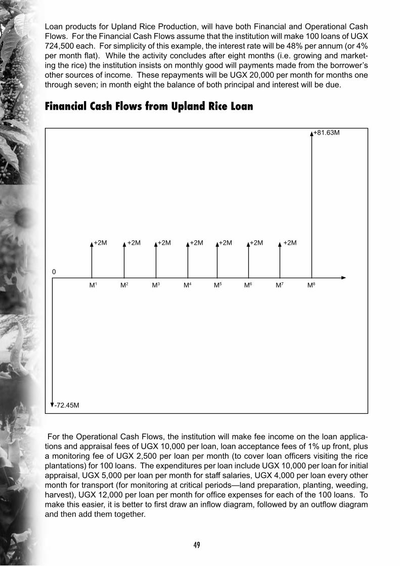
Loan products for Upland Rice Production, will have both Financial and Operational Cash Flows. For the Financial Cash Flows assume that the institution will make 100 loans of UGX 724,500 each. For simplicity of this example, the interest rate will be 48% per annum (or 4% per month flat). While the activity concludes after eight months (i.e. growing and market-ing the rice) the institution insists on monthly good will payments made from the borrower’s other sources of income. These repayments will be UGX 20,000 per month for months one through seven; in month eight the balance of both principal and interest will be due.

Financial Cash Flows from Upland Rice Loan

For the Operational Cash Flows, the institution will make fee income on the loan applica-tions and appraisal fees of UGX 10,000 per loan, loan acceptance fees of 1% up front, plus a monitoring fee of UGX 2,500 per loan per month (to cover loan officers visiting the rice plantations) for 100 loans. The expenditures per loan include UGX 10,000 per loan for initial appraisal, UGX 5,000 per loan per month for staff salaries, UGX 4,000 per loan every other month for transport (for monitoring at critical periods—land preparation, planting, weeding, harvest), UGX 12,000 per loan per month for office expenses for each of the 100 loans. To make this easier, it is better to first draw an inflow diagram, followed by an outflow diagram and then add them together.

+81.63M

-72.45M

0

+2M +2M +2M +2M +2M +2M +2M

M1 M2 M3 M4 M5 M6 M7 M8

49

Operational Inflows from Upland Rice Loan

Operational Outflows from Upland Rice Loan

Thus, combining the Operational Inflows with the Operation Outflows yields the Operational Cash Flow

Note carefully here that on the Operational Cash Flow the result is that the institution is cash flow negative on a monthly basis. Though this may look pessimistic, this is often the normal case. However, when considering both Financial and Operational Cash Flows, it becomes clear that the institution will have adequate liquidity throughout the loan cycle. Further, it must be noted that often Operational Expenses are paid out of Financial Income.

0 M1 M2 M3 M4 M5 M6 M7 M8

+.25M +.25M +.25M +.25M +.25M +.25M +.25M +.25M

+1.73M

0 M1 M2 M3 M4 M5 M6 M7 M8

-1M

-1.7M-2.1M

-1.7M-2.1M

-1.7M-2.1M

-1.7M-2.1M

M1 M2 M3 M4 M5 M6 M7 M8+.73M

-1.5M-1.9M

-1.5M-1.9M

-1.5M-1.9M

-1.5M-1.9M

0

51

Net Diagram for both Operational and Financial Cash Flows

Clearly the above diagram indicates that with this product structured as written, the institu-tion can meet its liquidity needs. However, it is also easy to see that with small changes in policies and procedures at the institution (for example lowering monitoring fees) this would not be true. This tool is very powerful in assisting the institution to determine its policies with respect to generating income and covering expense in such a way that volumes of cash and timing of cash enable the institution to always meet its obligations.

0 M1 M2 M3 M4 M5 M6 M7 M8

+.5M +.1M +.5M+.1M

+.5M+.1M

+.5M

+79.7

-71.72

53

Chapter VI

Risk Mitigation and the Affiliated Variable CostsBefore any lending decision on the part of a financial institution can be made, the loans officer and/or credit committee must assess each borrower’s willingness and capacity to repay. The best and easiest way to do this systematically is to apply the Five C’s of Lend-ing as described below. As with all activities, the financial institution must be conscious that evaluating a client will incur costs. These costs are largely variable costs because they are expensed on a loan-by-loan basis and as such should be paid by the particular borrower.

The Five C’s of Lending:

Character

Character reflects a borrower’s willingness to repay. Before making a loan, a lender must assess the borrower’s character by speaking to members of the community who know the borrower well, speaking to individuals and institutions that the borrower borrowed money from previously to assess if they were repaid without any problems, speaking to community leaders to assess if the borrower is considered an honest person, asking the borrower to provide guarantors who promise to repay his/her loan (and are capable of repaying his/her loan) in the event that the borrower defaults. Collecting this information on the borrower’s character requires the financial institution to incur some minimal variable costs during the loan appraisal. These costs are often best handled by charging the potential borrower a fee to appraise their loan.

Capacity

Capacity reflects a borrower’s Capacity to repay. Before making a loan, a lender must as-sess the borrower’s capacity by reviewing the borrower’s loan application and business plan. The lender will determine if the plan is feasible, well thought out, thorough, etc. The lender will further assess whether or not the borrower has done this type of business before. The lender will determine if the borrower has the necessary materials, skills, experience and experienced colleagues/employees to realize the success of the business he/she is borrow-ing for. Also the capacity to repay may be ascertained from the other viable activities the borrower is undertaking in addition to the business being loaned for. This review of capacity during appraisal will take time, effort and expense. Again, this cost should be borne by the potential borrower through the leveling of an appraisal fee.

Capital

Capital reflects both a borrower’s capacity and willingness to repay. Before making a loan, a lender must assess a borrower’s capital by reviewing the borrower’s loan application and business plan and verifying that the borrower has invested in the project the amount that he/she claims. If a borrower wants to borrow for a business or project,

that borrower should normally have at least 50% of the total costs for that project from their own assets. If a borrower is borrowing from another lender and then borrowing from your financial institution to cover the entire investment, this does not qualify. The borrower will be more serious when he/she has at least as much to lose as the lender. Appraising the

55

value of the potential borrower’s share of the investment will again cause the lender to incur some variable costs. These costs should be covered by the borrower and are best handled by leveling an appraisal fee to review the loan.

Collateral

Collateral reflects a borrower’s capacity and willingness to repay. Before making a loan, a lender must assess a borrower’s collateral by reviewing the borrower’s loan application and business plan and verifying that the borrower has the collateral that he/she claims. Collat-eral, as a matter for review, is any asset that the borrower pledges to the lender as payment in the event that the borrower defaults. Further, it is desirable for the lender that the bor-rower always pledges collateral. While the borrower may not have collateral with immediate cash value, he/she may pledge some objects of great personal value that they would rather not lose under any circumstance. The fear of losing such objects will compel the borrower to repay. Evaluating and/or encumbering the pledged collateral also represent a variable cost that the lender must cover by leveling a fee on the borrower.

Conditions

Conditions have an impact on the borrower’s capacity and willingness to repay. Conditions include economic conditions, political conditions, social conditions and environmental con-ditions that will influence the borrower’s success at investing his/her loan. Lenders must be aware of what impact external conditions might have on the borrower’s reliability and keep themselves informed as to market trends, etc.

Due Diligence

Finally as a matter of review, the concept of Due Diligence is another risk management tool. Due diligence is the concept that the lender must do everything in his/her power to make certain that a borrower is qualified to borrow before lending and that the borrower repays and repays according to the loan agreement. Application of due diligence includes using the five Cs of lending and using any other strategy to compel the borrower to honor the lending contract.

Interest Rate Determination

Recall that an interest rate for a loan contains five fundamental parts and that these parts can be further disaggregated into many more parts. The basic parts of an interest rate are “cost of funds (CF)”, “operational costs (OC)”, “inflation costs (IC)”, “loan loss costs (LLC)”, and profit. Of particular interest in risk management are the concepts of OC, IC and LL.

Operational Costs (OC) should reflect all costs of management. The lender should be certain to estimate and cover not only normal fixed management costs in OC, but also all variable costs associated with reviewing clients using the Five Cs; and, all costs associated with applying Due Diligence. The costs of screening, monitoring and penalizing borrowers (when necessary or appropriate) must be reflected in the OC.Loan Loss Costs (LLC) should reflect estimated loan losses. It may (and perhaps should) be different for different types of loans. Low-risk loans will have lower LLCs and hence lower overall interest rates. High-risk loans will have higher LLCs and hence higher overall interest rates.

57

Chapter VII

Loan Procedures and CostsIn the previous chapter, the concept of due diligence was presented. This chapter builds on that background to cover the costs involved in appraising, delivering and recovering ag-ricultural loans.

Development of an agricultural loan product is incomplete unless procedures and mecha-nisms for delivery of the product are stipulated and incorporated. Procedures and mech-anisms refer to the ‘hows’ the loan product will be effectively delivered, right from client screening to disbursement, monitoring and recovery of the loan, including provision for mak-ing repeat loans to the borrower. It refers to what both the lender and the borrower ought to do to facilitate the delivery of the agricultural loan product.

Each procedure has implications on both cost and time, and therefore has relevancy to the loan interest and charges if the product is to be viable. There are both direct and indirect costs related to the respective loan procedures. Thus for the financial institution, it is im-perative that the agricultural loan product procedures be cost-effective and optimize loan decision time.

Application and CostsThe prospective client must apply for the loan and must be screened as a potential bor-rower. The cost associated with the application process is largely the time for the screening interview, except where the prospective applicants have to be solicited by the staff which may involve transport and other field costs. The loan application form costs are recoverable from the sale of the form to the applicant.

Appraisal and CostsDetailed project and borrower appraisal is very important in making a rational agricultural lending decision. Site and applicant’s home visits are crucial for effective appraisal. This necessarily involves transport and other in-field costs. The number of applications appraised and the total value of loans accessible on a single visit impact the average loan appraisal cost and the cost per loan. Thus repeat loans and a bigger number of applications ap-praised on a single visit lower the appraisal costs. The appraisal procedures should enable the assessment of the repayment capacity of the agricultural business to be funded, the capacity of the applicant to repay the loan, including assessing and securing documenta-tion for the proposed collateral. It is at this point that the five Cs of lending, presented in the previous chapter are effectively applied.

Approval and CostsThe approval procedures relate to the loan decision process and are just intended to test the effectiveness and completeness of the appraisal process. It is normally by a consti-tuted panel or loan committee to which the loan officer presents the application appraisal for concurrence. Thus the relevant costs are those related to the time spent by the committee on a loan case presented and also the costs relating to collateral registration. However, the latter costs are directly recoverable from the borrower on disbursement of the loan and thus need not be considered.

59

Disbursement and CostsAn approved agricultural loan should be timely and appropriately disbursed to the borrower to minimize delayed performance and the risk of the borrower diverting the money from the loan to some other purpose. It is prudent to disburse the loan according to the schedule of the proposed activities to be accomplished. On disbursement a proper loan agreement should be signed by the borrower and the manager and witnessed. The costs involved here are largely overheads relating to staff time and stationery.

Monitoring and CostsAgricultural businesses need closer monitoring than other types of loans. Any omission or delay in execution of any activity impacts on the overall outcome of the business and affects the loan repayment capacity. For example if a farmer accesses a loan for rice production but fails apply fertilizer either because the fertilizer is unavailable in the market or the loan funds have been diverted, the expected yield will certainly not be realized. Similarly if weed-ing is either not done at all or is not done on time, the yield will be lower. Therefore, there is need for effective monitoring of the funded agricultural businesses if the risk of default due to poor performance of the business is to be minimized or avoided.

However, monitoring involves costs as it has to be done at the site of the business to en-sure that everything is being done as initially planned. The major costs are transport and in-field expenses. The greater the number of monitoring visits undertaken the more will be the costs. Therefore, it is important to monitor only the critical stages such as at planting to ensure that the right inputs have been used, at weeding to ensure that the weeding activ-ity has been done on time and at harvest to ensure that the crop has been harvested and therefore verify the certainty of sales proceeds.

As earlier pointed out, if there are many agricultural loans extended in a given location, any single monitoring can cover more than one client and thus help to spread the monitoring costs and lower the average cost per loan.

It is important that the monitoring be documented and filed for future reference as the activ-ity progresses. It may be necessary for the borrower to countersign the monitoring notes to avoid future counter accusation about what was done or not done that led to problems in repayment.

Recovery and CostsRecovery of loans, especially those in default, can be a tedious and costly undertaking. Hence there is a need to avoid loans in arrears as much as possible through undertaking careful application appraisal, setting appropriate loan terms, carrying out effective monitor-ing and building sound client relationships that foster willful loan repayments. The recovery costs relate to transport and telephone services while trying to secure the recovery and, collateral disposition costs and legal costs in the case of loans in default.

Sample Guidelines and Procedures for Agricultural Production Loan Product

Eligibility/Client Selection Procedure1. The applicant should be engaged in the production of the crop or livestock for

which the loan product is on offer.

61

2. The applicant must have no any outstanding loans with the financial institution be-fore applying for the agricultural loan.

3. The applicant should have experience of at least two years in the farming activ-ity for which a loan is required. She or he should have evidence that the farming activity is profitable and uses improved agronomical practices to improve on the quantity and quality of production.

4. The applicant should own land used for agricultural production or have verifiable proof of authority to use it.

5. The applicant should demonstrate capacity to provide reasonable matching equity for the activity to be funded.

6. If any of the above requirements is not met, the loans officer will have the preroga-tive to advise the applicant not to pursue the loan any further. If the prospective applicant doesn’t agree with the loan officer, she or he can seek manager’s audi-ence who, together with the loan officer, will enter a final verdict on whether or not the application can processed further.

Application Procedure

1. If the eligibility criteria are satisfied, the agricultural loans officer advises the appli-cant to purchase the specific application form for agricultural loans.

2. The loans officer assists the applicant to complete the loan application form.

3. The agricultural loans officer schedules with the applicant the actual day to visit the farm/business to appraise the application.

Loan Assessment/Appraisal Procedure

1. The loan officer visits the applicant’s farm/business and residence on a date agreed.

2. The loan officer gathers financial and social economic data about the proposed and other businesses of the applicant, as detailed in the agricultural loan application form, photographs of the business, photographs of the applicant’s residence and details of proposed collateral.

3. Data collected by the loan officer, including costs, prices and income (dully verified for accuracy and reliability) is analyzed in the form of an income statement and cash flow projection covering the whole agricultural production period of the enter-prise to be funded.

4. The loan officer uses analyzed data to estimate the capacity of the applicant to pay and determines the appropriate loan terms including loan amount, loan period and repayment installments.

5. The loan officer prepares a loan application summary for presentation to the loans committee.

63

Loans Committee Decision Procedure

1. All agricultural loans must be approved by a loans committee consisting of the chair-person, credit supervisor/senior credit officer and one or more credit officer.

2. The loan officer presents a summary page of the completed loan application form photocopied and distributed to all loans committee members at least 6 to 12 hours before the meeting.

3. The loans officer who made the appraisal leads the discussion and presents the recommendation on the loan application as per summary sheet information.

4. The committee members verify the correctness of the presentation by asking ques-tions on the enterprise to be financed as well as the applicant. It is important that committee members are familiar with the general background of the farming ac-tivities of the area such as yield, the risks therein, the prices and market trends in order to avoid accepting an over optimistic presentation from the loans officer.

5. When the committee members are convinced, they individually sign on the loan summary sheet. No single individual is allowed to make a loan decision, but loan decisions will be made unanimously. There is no exception to this rule. All the members of the loan committee will sign the committee summary.

Disbursement Procedure 1. A documentation checklist is completed by the manager verifying and ensuring that

all the documents have been properly filed and signed and the listed collateral pro-vided.

2. The manager, on being satisfied that all the loan conditions have been fulfilled, au-thorizes the disbursement of the loan.

3. Prior to disbursement it is important to ensure that:

a. Loan agreements are fully signed by the borrower, manager and witness. Note that the loan agreement must have the repayment schedule annexed to re-mind the borrower the due dates for the repayment of installments.

b. The committee summary is duly signed and has the appropriate loan authori-zation.

c. The loan collateral is properly documented, with the necessary encumbrances entered.

Monitoring Procedure 1. The loan officer shall visit the applicants business at least three times during the

tenure of the loan, at the critically identified stages in the production cycle.

2. During the monitoring, the loan officer shall particularly ensure that the borrower applied the loan funds on the activity funded in a manner that renders the attain-ment of maximum yield possible.

3. In case of detection of diversion of loan funds by the borrower, the loan officer will recommend a recall of the loan.

65

4. The loan officer shall document the monitoring observations on each monitoring visit that will be filed in the loan file. The borrower will countersign the monitoring notes.

Recovery Procedure

1. A week to the due date of the installment, the loan officer notifies the borrower of the need to pay the installment.

2. If any installment falls in arrears, the loan officer must immediately communicate to the borrower and point out the penalties involved in loan arrears. The loan officer arranges for a visit to the borrower for installment recovery.

3. If the borrower refuses or is unable to pay, the loan officer initiates the forced re-covery process, including liquidation of collateral and legal action.

4. In case of forced recovery, all recovery costs must be transferred to the borrower.

Note on rescheduling, write offs and early repayments:

Not all loans or installments must be repaid when they fall due. There are instances when the borrower may genuinely not be able to pay one or a number of installments when they are due as a result of existing circumstances such as delayed marketing of the commodity. In this case, the loan should be rescheduled but the interest must continue to accrue.

Also there may be a possibility where a borrower generates capacity to repay the loan ahead of its maturity. In such cases it may be reasonable to restructure the repayment plan and reschedule the installments or accept early retirement of the loan. Rescheduling the repayment needs to be negotiated ahead of the due date and thus require a continuous assessment of client’s capacity to repay the installments through maintaining close contact with the loan officer. Similarly where the borrower requests for early retirement of the loan, for example in case of marketing the commodity ahead of the anticipated timing or where the borrower accesses funds from other sources, such a request should be granted at no penalty save for a reasonable administrative charge. In the extreme where it is certain that a loan in arrears cannot be recovered, it is prudent to write off the loan rather than pursue recovery which adds further costs and thus losses and also distorts the portfolio quality.

67

Chapter VIII

Product Costing and Interest Rate Determination:Background

There are essentially two methods to setting interest rates. The first, and easier, method is to review the interest rates charged by competitors for the same or similar products and determining if by charging that interest rate (or slightly less) the institution can be profitable. The second method is to determine every cost that is incurred in delivering a product and designing the interest rate and attached fees to cover all of those costs and leave some margin for the institution. While in Uganda, the most common way of setting interest rates is the first, it is not the better way of doing this critical task. There are many reasons for this:

6 Competition is relatively rare (1 in 10 Ugandans are banked) so determining inter-est rates based on perceived competitors is flawed logic;

6 Cost accounting skills are weak and this leads to underestimated delivery costs.

6 For member-based institutions, one of the driving goals is service at cost to the members; therefore it is always preferable to determine the costs first.

6 There is no guarantee that the competitor is charging an interest rate which covers their internal costs.

Product Costing

In order for a financial product to be viable it must achieve full delivery cost recovery, produce profit and minimize risk to the institution. There are many ways to disaggregate the various costs of delivering a financial product from an institution. One of the simplest scientific ways to do this is by categorizing the costs into four broad categories. These are:

1. Cost of Funds (CF),

2. Operational Costs (OC),

a. Fixed,

b. Variable

3. Inflation Costs (IC), and

4. Loan Loss Costs (LLC)

In addition to these four costs, the institution must also consider a profit margin to help it to both grow and produce prosperity for the shareholders. After accounting for the product costs and profit margin, the interest rate charged to the borrower for a given product can be determined:

Interest Rate = CF+OC+IC+LLC+Profit

69

Cost of Funds (CF):

CF is what the financial institution must pay to receive adequate lending capital (refer back to the discussion of Offsetting Liabilities). There are many methods of funding a loan prod-uct. These include (from least costly to most costly) funding from compulsory deposits, funding from fixed deposits, funding from voluntary deposits, funding from subsidized loans, funding from wholesale commercial loans, funding from reserves, funding from non bank lenders. The financing plan for a loan product must clearly indicate where the funding for the product is coming from and the costs of that funding must be determined in terms of an annual percentage rate. If there are multiple sources, the sources must be weighted and averaged (this will be demonstrated in the example at the end of this chapter).

Operational Costs (OC)

OC is what the financial institution must pay to cover the costs of delivering, monitoring and recovering the loan. OC must also cover the overhead expenses of maintaining the physical structure and staff of the financial institution. These overheads must be properly allocated over each financial product the institution offers. OC is normally divided into both fixed costs and variable costs. The fixed costs include the overheads and ongoing costs (which must be paid whether or not any loan is made). The variable costs include all costs incurred spe-cifically to deliver, monitor and recover that particular loan product including staff costs for reviewing the application, initial field appraisal, disbursement costs, field follow up monitor-ing, anticipated visits to eliminate arrears, etc.). As with CF, these costs must be determined in terms of an annual percentage rate (this will also be covered in the example at the end of this chapter).

Inflation Costs (IC)

IC is what the financial institution must pay to cover the loss of the value of the money they lend to their clients. Everyone is aware that what a shilling buys today is less than what a shilling bought five years ago. This is the effect of inflation (money is losing its value rela-tive to the costs of goods and services). The rate of inflation is nationally determined and is available from the Bank of Uganda. It is based on an annual percentage rate and does not require conversion (this will also be covered in the example at the end of this chapter).

Loan Loss Costs (LLC)

LLC is what the financial institution must pay to cover the anticipated losses from loan de-faults which result in write offs. This can be determined over several loan cycles (the institu-tion may learn for example that on dairy loans, 5% of the amount loaned is never recovered for one reason or another). Before there is any real experience in determining loan losses, it is best to over estimate what those losses might be (this will also be covered in the example at the end of this chapter).

Profit

Profit is what the financial institution plans for its own growth and for the benefit of its owners (shareholders, etc.). It is best to plan a profit margin in every loan product in order to have a good estimate ex ante of what the institution will be able to earn and distribute as dividends. Again, this figure should be on an annual percentage rate basis (this will also be covered in the example at the end of this chapter).

71

Interest Rate Determination Example of Upland Rice

Assume that the financial institution determines that the cost for a borrower to grow one acre of upland rice is UGX 1,000,000. The term of the loan will be 8 months including production, harvesting and marketing. In following prudent lending standards, the institution expects that the borrower will provide 50% of the necessary investment. Therefore, the institution determines that each upland rice loan will be UGX 500,000. As with previous examples, the institution will make 100 of these loans for a total portfolio of UGX 50M.

Cost of Funds (CF)

To determine its interest rate, the institution must look at its CF, IC, OC, LLC and profit. To cover its CF, the institution will use a combination of savings and borrowing. The institution has savers to whom they must pay 10%/annum for fixed deposits worth UGX 25M (in order to meet this obligation the institution must accrue enough income over the course of the year). In addition, the institution will borrow UGX 25M from a wholesale lender at 18%/an-num which is payable in two-six month installments of both principal and interest4 . To deter-mine the CF, the institution must take the weighted average of these two sources of funds.

Operational Costs (OC)

The institution must also look at its fixed and variable OC to further specify its interest rate. In terms of fixed costs, the institution has the following annual costs (payable on a monthly basis): Management Salaries (Indirect Staff Time) UGX 20M, Rent UGX 5M, Utilities and Services UGX 3M, Other Overheads UGX 2M. This loan will represent 10% of the institu-tion’s total loan portfolio.

In addition to fixed costs, actually making each loan has the following variable costs: Paper-work UGX 10,000 before the loan is released, Field Appraisal Expenses UGX 4,000 before the loan is released, Loan Monitoring Costs UGX 4,000 in months 2, 4 and 8, Direct Staff Time UGX 20,000 (spread over the eight month period). In addition to these costs, the insti-tution will consult an extension agent specialized in rice at a cost of UGX 2,000/loan during the appraisal before the loan is released. To determine the interest rate, both the fixed and variable OCs must be determined on an annual percentage rate basis.

Inflation Cost (IC)

In consulting the Bank of Uganda, the IC is found to 5%/annum.

Loan Loss Costs (LLC)

Because this is a new product, and the institution has experience in launching other new products, based on that experience, the institution will expect losses of 3.5% of the amount loaned in the first year.

4 Wisely, both sources of funds (which are offsetting liabilities) are relatively stable in that half the loan will not come due for a year and the savings must only be paid back after one year. However, the institution must be careful to pay off half of the loan after six months.

73

Profit

After covering all costs, the institution is seeking a 6%/annum return on their agricultural loans.

Determining the Interest Rate

CF

The total portfolio for this product will be UGX 50M. The institution will get UGX 25M from fixed savings deposits at 10%/annum; and UGX 25M from a bank loan at 18%/annum. To find the CF, the institution will take the average of these two values as follows:

CF = (UGX 25M ÷ UGX 50M) x 10%/annum + (UGX 25M ÷ UGX 50M) x 18%/annum

CF = 14%/annum

OC

The total fixed costs for the institution are UGX 30M/annum of which 10% are allocated to this loan product. Therefore, UGX 30M/annum _ 10% = UGX 3M (given 100 loans, this works out to UGX 30,000/loan). The variable costs per loan are a total of UGX 48,000. The institution must express the sum of these costs as a percentage of the value loaned. The total of each loan is UGX 500,000. Therefore, the OC is found as follows:

OC = (UGX 30,000 ÷ UGX 500,000) x 100%/annum + (UGX 48,000 ÷ UGX 500,000) x 100%/annum

OC = 15.6%/annum

IC

This is given as 5%/annum by the Bank of Uganda

IC = 5%/annum

LLC

LLC is estimated to be 3.5%/annum based on previous experience.

LLC = 3.5%/annum

Profit

As discussed above, the institution expects a profit of 6%/annum on this product.

Profit = 6%/annum.

75

Recall that,

Interest Rate = CF+OC+IC+LLC+Profit

Therefore,

Interest Rate = 14% + 15.6% + 5% + 3.5% + 6% = 44.1%/annum

This is a good way to start looking at the product viability. All costs have been identified and planned for in the interest rate. However, recall that on the basis of the cash flow analysis chapter, it is not enough to know how the large the inflows and outflows are; the institution must also be conscious of precisely when they will materialize. Otherwise there will not be adequate liquidity to meet the institution’s obligations.

Re-Evaluate the Expected Cash Flows to Verify Institution’s Capacity to Provide the Product

In order to better understand the timing the cash flows, the institution must review when it expects its inflows and outflows on the basis of the five parts of its interest rate. Based on the example above, the institution can develop the following cash flow diagrams:

CF

Recall that the CF is based on two parts. These are a fixed deposit savings liability payable at the end of 12 months at 10% annual interest and a loan liability at 18% annual flat interest payable in two equal six month installments.

Fixed Deposit:

0

M1 M2 M3 M4 M5 M6 M7 M8 M9 M10 M11 M12

+25M

-27.5M

MONTH

77

Commercial Loan:

Combining these for the total CF cash flow, the institution finds the following:

OC

-14.75M

0

M1 M2 M3 M4 M5 M6 M7 M8 M9 M10 M11 M12

+25M

-14.75M

MONTH

0

M1 M2 M3 M4 M5 M6 M7 M8 M9 M10 M11 M12

+50M

-42.25M

-14.75M

MONTH

79

The institution now must break down the OC according to fixed and variable costs to de-termine the timing of these cash flows. Recall that the total fixed costs attached to making the loan are payable on a monthly basis and are UGX 30M per year. This represents a monthly cost of 2.5M Further the variable costs per loan are as follows: at disbursement UGX 16,000/loan; each month UGX 2,500/loan and in months 2, 4 and 8 an additional UGX 4,000/loan. Therefore, for 100 loans the figures are: UGX 1.6M at disbursement, UGX 250,000 per month except in months 2, 4 and 8 when the costs will be UGX 650,000.

Fixed Cost Cash Flows

Variable Cost Cash Flows

Therefore, for 100 loans the figures are: UGX 1.6M at disbursement, UGX 250,000 per month except in months 2, 4 and 8 when the costs will be UGX 650,000.

0 M1 M2 M3 M4 M5 M6 M7 M8 M9 M10 M11 M12

-25M -25M -25M -25M -25M -25M -25M -25M -25M -25M -25M -25M

MONTH

0 M1 M2 M3 M4 M5 M6 M7 M8 M9 M10 M11 M12

-25M -25M -25M -25M -25M -25M -25M -25M -25M -25M -25M -25M

MONTH

0 M1 M2 M3 M4 M5 M6 M7 M8 M9 M10 M11 M12

-1.5 -0.25 -0.65 -0.25 -0.65 -0.25 -0.65 -0.25 -0.65 MONTH

81

Combining these for the total OC cash flow, the institution finds the following:

IC, LLC and Profit:

These three items are accrual items and therefore have no precise cash flows that the insti-tution must consider in order to meet its obligations.

Combined Cash Flows

All of the expense related cash flow diagrams can be combined into a single expense cash flow as shown below.

The cash flow diagram above tells the financial institution what cash it needs at what time to service the costs of delivering this loan product for upland rice. This diagram again can be combined with an income cash flow diagram.

Income Cash Flow Diagram

Remember that the institution is borrowing UGX 25M from a lender and raising UGX 25M in fixed deposits. Beyond this assume that the institution receives application fees of UGX 5,000 per loan and a one time full repayment of principal and interest after eight months. If we have 100 loans of UGX 500,000 earning interest of 44.1% annually or 3.7% monthly the cash flow for this income will appear as follows:

-50M

0 M1 M2 M3 M4 M5 M6 M7 M8 M9 M10 M11 M12

-2.75 -3.15 -2.75 -2.75-3.15

-17.5

-2.75 -3.15

-42.25M

MONTH

83

0 M1 M2 M3 M4 M5 M6 M7 M8 M9 M10 M11 M12

-1.6 -2.75 -3.15 -2.75 -3.15 -2.75 -2.75 -3.15-2.75 MONTH

Combining the income and expense cash flow diagrams, we get the following result:

0 M1 M2 M3 M4 M5 M6 M7 M8 M9 M10 M11 M12

+64.8M

+50.5M

MONTH

M1 M2 M3 M4 M5 M6 M7 M8 M9 M10 M11 M12

+50.5M

0

+61.65M

-17.5M

-42.25

-2.75-2.75-2.75-2.75 -3.15 -3.15 MONTH

85

Chapter X

Product Promotional StrategyOnce the agricultural loan product has been designed and tested, and the financial institu-tion is confident of rolling it out on the market, there is need to market or promote it. Product promotion entails raising the public awareness of the existence of the loan product within the financial institution. This takes many forms ranging from print and broadcast media, radio communication to word of mouth.

The marketing approach adopted has implications in terms of outreach effectiveness, mar-keting costs and potential loan revenue to be generated. There is therefore need to develop a strategy to optimize these variables and thus realize bigger impact. Focusing on only one aspect such as cost may not be ideal. Again the characteristics of the target market, as de-termined by demand analysis and enterprise selection, should assist in adopting an effective promotional strategy. For instance if the access to television in the locality is limited due to either lack of electricity or broadcast facilities, it is not worthwhile advertising the prod-uct on television. Similarly if the readership of newspapers in the rural area of the product market focus is poor, any promotion through newspapers will be wasted and may not create the desired impact. In the case of promotion through radio, the timing of the promotion is equally important. Agricultural enterprises, especially those in production, may not access radio during the day when producers are busy in their fields. Thus radio promotion for an agricultural product may best be done in the evening or at night when the availability of the intended audience is certain.

From the above explanation it is clear that the financial institution intending to promote an agricultural loan product must plan and adopt an effective promotional strategy that will ensure realization of impact as will be measured by the number of loans sought in a given period of time. The impact needs to be monitored and where necessary the marketing strat-egy evaluated for possible adjustment.

Printed promotional materials that can be distributed, pinned on strategic places including in the banking hall of the financial institution have a bigger effect of carrying the message to the intended audience. Also direct personal contact through promotional meetings, semi-nars and mini workshops at which the product features and the institution’s procedures are explained can equally be very effective.

The promotional message needs to very clear so that it is easily communicated to the in-tended recipients. Language, content, general presentation and color play a big role. The information in the promotional material should be brief, specific and in the language under-stood by the recipients. Inclusion of a relevant photograph may create additional attraction potential. The information conveyed should target at arousing interest of the potential bor-rower rather than explain all the loan product details.

For effectiveness, the loan product marketing strategy should be underpinned by a well thought out promotional budget. More often there is a remarkable tendency to allow for a lower promotional budget for a new loan product owing to the perceived uncertainty of the product and thus its capacity to generate sustainable income. If the demand analysis was adequately undertaken and proper product design achieved, such mystic perception within the institution ought to be minimized.

87

Chapter XI

Product Re-EvaluationAs discussed in Chapter I, a product is only viable if it both satisfies the needs of the bor-rower and lender. This entire manual is largely dedicated to evaluating the lenders needs. However, a financial institution would be short sighted to look only at covering its costs with-out evaluating whether or not a client would want the product. In essence, a client will only borrow if she or he can repay and remain with a reasonable profit for their efforts.

Following the example of upland rice, we know from the previous chapter that the financial institution must charge at least 44.1% annually to mitigate its risks, cover its costs and earn a reasonable profit on this product. Recall from chapter III that the value chain mapping exercise revealed the following:

This shows that the client in eight months will earn 107% on his investment in eight months which annualizes to 161%. Therefore, the borrower can easily pay 44.1% in interest and remain highly profitable.

Therefore, if the institution is considering this product and has properly costed all of the rel-evant parts to delivering this product, it should decide to offer this product to its clients.


yield)

Value Per KG




Investment


Total Costs of Production Before Financing

(90,000.0)(151,000.0)(88,000.0)

(140,000.0)(14,000.0)

(183,000.0)

(45.0)(75.5)(44.0)(70.0)(7.0)

(211.5)


89

a comprehensive guide to agricultural …pdf.usaid.gov/pdf_docs/pnadl008.pdfa comprehensive guide to...

Documents