a comprehensive mathematical model for the design of cellular manufacturing systems
TRANSCRIPT

ARTICLE IN PRESS
0925-5273/$ - see
doi:10.1016/j.ijp
�Correspondifax: +1514 848
E-mail addre
Int. J. Production Economics 103 (2006) 767–783
www.elsevier.com/locate/ijpe
A comprehensive mathematical model for the design of cellularmanufacturing systems
Fantahun M. Defersha, Mingyuan Chen�
Department of Mechanical and Industrial Engineering, Concordia University, 1455 Maisonneuve West, Montreal, Que., Canada H3G 1M8
Received 9 July 2004; accepted 30 October 2005
Available online 13 June 2006
Abstract
The design of cellular manufacturing systems (CMS) involves many structural and operational issues. One of the
important design steps is the formation of part families and machine cells. In this paper, a comprehensive mathematical
model for the design of CMS based on tooling requirements of the parts and tooling available on the machines is proposed.
The model incorporates dynamic cell configuration, alternative routings, lot splitting, sequence of operations, multiple
units of identical machines, machine capacity, workload balancing among cells, operation cost, cost of subcontracting part
processing, tool consumption cost, setup cost, cell size limits, and machine adjacency constraints. Numerical examples are
presented to demonstrate the model and its potential benefits.
r 2006 Elsevier B.V. All rights reserved.
Keywords: Cellular manufacturing; Dynamic cell configuration; Alternate routings; Lot splitting; Workload balancing; Integer
programming
1. Introduction
A cellular manufacturing system (CMS) is aproduction approach aimed at increasing produc-tion efficiency and system flexibility by utilizing theprocess similarities of the parts. It involves groupingsimilar parts into part families and the correspond-ing machines into machine cells. This results in theorganization of production systems into relativelyself-contained and self-regulated groups of ma-chines such that each group of machines undertakean efficient production of a family of parts. Such
front matter r 2006 Elsevier B.V. All rights reserved
e.2005.10.008
ng author. Tel.: +1514 848 2424x3134;
3175.
ss: [email protected] (M. Chen).
decomposition of the plant operations into sub-systems may often lead to reduced paper work,reduced production lead time, reduced work-in-process, reduced labor, better supervisory control,reduced tooling, reduced setup time, reduceddelivery time, reduced rework and scrap materials,and improved quality (Wemmerlov and Johnson,1997).
In the last three decades, research in CMS hasbeen extensive and literature in this area isabundant. Comprehensive summaries and taxo-nomies of studies devoted to part-machine groupingproblems were presented by Wemmerlov andHyer (1986), Kusiak (1987), Selim et al. (1998),and Mansouri et al. (2000). Methods for partfamily/machine cell formation can be classified as
.
ARTICLE IN PRESS
Table 1
List of manufacturing attributes
1. Alternative routing
(a) Selecting the best route
(b) Allowing alternative routing coexist
2. Demand fluctuation
(a) Deterministic
(b) Probabilistic
3. Dynamic cell reconfiguration
4. Workload balancing
(a) Inter-cell workload
(b) Intra-cell workload
5. Lot-splitting
6. Types of tools required by a part
7. Types of tools available on a machine
8. Machine proximity constraint
(a) Separation constraint
(b) Collocation constraint
9. Sequence of operation
(a) Used as input for determine magnitude of material flow
(b) Used as similarity measure between parts
10. Setup cost/time
(a) Setup cost
(b) Setup time
11. Cell/part family size constraint
(a) Cell size constraint
(b) Part family size constraint
12. Movement of parts (material handling cost)
(a) Inter-cell movement
(b) Intra-cell movement
13. Facility layout
(a) Inter-cell layout
(b) Intra-cell layout
14. Operator allocation
15. Machine capacity
16. Identical machines
(a) Within a cell
(b) In the entire system
17. Machine investment cost
18. Subcontracting cost
19. Tool consumption cost
20. Unit operation time
21. Operation cost
F.M. Defersha, M. Chen / Int. J. Production Economics 103 (2006) 767–783768
design-oriented or production-oriented. Design-or-iented approaches group parts into families basedon similar design features. An overview of design-oriented approaches based on classification andcoding was presented by Askin and Vakharia(1990). Production-oriented techniques are foraggregating parts requiring similar processing.These approaches can be further classified intocluster analysis, graph partitioning, mathematicalprogramming, artificial intelligence (AI) basedapproaches, and heuristics (Greene and Sadowski,1984; Joines et al., 1996).
Mathematical programming is widely used formodeling CMS problems. The objective of themathematical programming model is often tomaximize the total sum of similarities of parts ineach cell, or to minimize inter-cell material handlingcost. Purcheck (1974) applied linear programmingtechniques to a group technology problem. Kusiak(1987) proposed the generalized p-median modelconsidering the presence of alternative routings.Shtub (1989) used the same approach and reformu-lated the problem as a generalized assignmentproblem. Wei and Gaither (1990) developed a 0–1programming cell formation model to minimizebottleneck cost, maximize average cell utilization,and minimize intra-cell and inter-cell load imbal-ances. The bottleneck cost is related to the proces-sing of bottleneck parts. Rajamani et al. (1990)proposed three integer programming models toconsider budget and machine capacity constraintsas well as alternative process plans. Askin and Chiu(1990) proposed a cost-based mathematical formu-lation and a heuristic graph partitioning procedurefor cell formation. Shafer and Rogers (1991) applieda goal programming method to solving CMSproblems for different system reconfiguration situa-tions: setting up a new system and purchasing allnew equipment, reorganizing the system using onlyexisting equipment, and reorganizing the systemusing existing and some new equipment. Shaferet al. (1992) presented a mathematical programmingmodel to address the issues related to exceptionalelements. Heragu and Chen (1998) developed amathematical programming model for cell forma-tion and used Benders’ decomposition to solve theproblem.
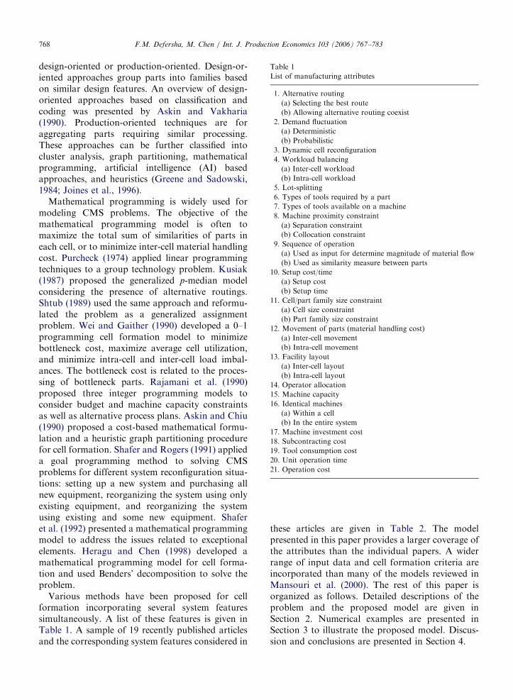
Various methods have been proposed for cellformation incorporating several system featuressimultaneously. A list of these features is given inTable 1. A sample of 19 recently published articlesand the corresponding system features considered in
these articles are given in Table 2. The modelpresented in this paper provides a larger coverage ofthe attributes than the individual papers. A widerrange of input data and cell formation criteria areincorporated than many of the models reviewed inMansouri et al. (2000). The rest of this paper isorganized as follows. Detailed descriptions of theproblem and the proposed model are given inSection 2. Numerical examples are presented inSection 3 to illustrate the proposed model. Discus-sion and conclusions are presented in Section 4.

ARTICLE IN PRESS
Table 2
Attributes used in the present study and in a sample of recently published articles
Article/Attributes 1 1 2 2 3 4 4 5 6 7 8 8 9 9 10 10 11 11 12 12 13 13 14 15 16 16 17 18 19 20 21 Total attr.
a b a b a b a b a b a b a b a b a b a b
Present study (this paper) � � � � � � � � � � � � � � � � � � � � � 21
Cao and Chen (2004) � � � � � � 6
Jayaswal and Adil (2004) � � � � � � � � � � 10
Solimanpur et al. (2004) � � � � � � � � � � 10
Xambre and Vilarinho (2003) � � � � � � � 7
Asokan et al. (2001) � � � � � � � � 8
Baykasoglu et al. (2001) � � � � � � � � � � � � 12
Diaz et al. (2001) � � � � � � � 7
Onwubolu and Mutingi (2001) � � � 3
Akturk and Turkcan (2000) � � � � � � � � � � � � 12
Caux et al. (2000) � � � � � � � � 8
Mungwattana (2000) � � � � � � � � � � � � � 13
Plaquin and Pierreval (2000) � � � � � 5
Zhao and Zhiming (2000) � � � � � � � � � 9
Sofianopoulou (1999) � � � � � � 6
Wicks and Reasor (1999) � � � � � � � � � � � 11
Chen (1998) � � � � � � 6
Heragu and Chen (1998) � � � � � � � � � � 10
Selim et al. (1998) � � � � � � � � � � � � � � 14
Su and Hsu (1998) � � � � � � � � � � � � � 13
Note: Attributes’ names are referred in Table 1.
F.M. Defersha, M. Chen / Int. J. Production Economics 103 (2006) 767–783 769
2. The mathematical model
2.1. Problem description
Consider a manufacturing system consisting of anumber of machines to process different parts. Eachmachine has a number of tools available on it and apart may require some or all of the tools on a givenmachine. A part may require several operations in agiven sequence. An operation of a part can beprocessed by a machine if the required tool isavailable on that machine. If the tool is available onmore than one machine type then the machines areconsidered as alternative routings for processing thepart. An entire lot of a part may split into differentcells for the processing of an operation. Themanufacturing system is considered for a numberof time periods. Each machine has a limitedcapacity expressed in hours during each time period.Machines can be duplicated to meet capacityrequirements and to reduce or eliminate inter-cellmovement. If additional machines are required in agiven time period, the machines can be procuredwith certain limit. Assume that the demands for thepart processing vary with time in a deterministicmanner. Further assume that the processing, setup,
and tool consumption costs do not depend on theplanning period. Machines are to be grouped intorelatively independent cells with minimum inter-cellmovement of the parts. In grouping the machines, itis also required that the workload of the cells shouldbe balanced. Machines that cannot be located in asame cell due to technical and environmentalrequirements should be separated. Machine pairsthat utilize common resources are required to belocated in the same cell. To address this multipletime period cell formation problem, a mixed integerprogramming model is formulated. The objective ofthe model is to minimize machine maintenance andoverhead cost, machine procurement cost, inter-celltravel cost, machine operation and setup cost, toolconsumption cost, and system re-configuration costfor the entire planning time horizon. The notationsused in the model are presented below.
Indices:
Time period index: t ¼ 1; 2; . . . ;TPart type index: i ¼ 1; 2; . . . ; IIndex of operations of part i: j ¼ 1; 2; . . . ; Ji
Machine index: k ¼ 1; 2; . . . ;KTool index: g ¼ 1; 2; . . . ;GCell index: l ¼ 1; 2; . . . ;L

ARTICLE IN PRESSF.M. Defersha, M. Chen / Int. J. Production Economics 103 (2006) 767–783770
Input data:
diðtÞ
demand for part i in time period tVi
unit cost to move part i between cells Bi batch size of product iFi
cost of subcontracting part iljig ¼ 1
if operation j of part i requires tool g, 0otherwisedgk ¼ 1
if tool g is available on machine k, 0otherwisehjik
processing time of operation j of part i onmachine type kwjik
tool consumption cost of operation j ofeach part i on machine type kmjik
setup cost for operation j of part i onmachine type kQkðtÞ
maximum number of machine type k thatcan be procured at the beginning of period tPkðtÞ
procurement cost of machine type k atthe beginning of period tHk
maintenance and overhead costs ofmachine type k per time period tOk
operation cost per hour of machine type kCk
capacity of one machine of type k for onetime periodLBl
minimum number of machines in cell lUBl
maximum number of machines in cell lIþk
cost of installing one machine of type kI�k
cost of removing one machine of type kq
0pqo1; a factor for the workload of acell being as low as q� 100% from theaverage workload per cellZiðtÞ
the number of cells among which anentire lot of part i may split into duringtime period t for the processing of certainoperations; ZiðtÞ 2 f1; 2; . . . ;LgM
a large positive number S a set of machine pairsfðka; kbÞ=ka; kb
2 f1; . . . ;Kg; kaakb,andka cannot be placed in the same cell with
kb}
O a set of machine pairs fðkc; kdÞ=
kc; kd2 f1; . . . ;Kg; kcakd , and kc should
be placed in the same cell with kdg
Decision variables:General integer:
NklðtÞ
number of type k machines to assign to celll at the beginning of period tyþklðtÞ
number of type k machines to add to cell lat the beginning of period t
y�klðtÞ
number of type k machines to remove fromcell l at the beginning of period tContinuous:
ZjiklðtÞ
the proportion of the total demand ofpart i with the jth operation to performby machine type k in cell l duringperiod tZiðtÞ
the proportion of the total demand of parti to be subcontracted in time period tAuxiliary binary variables: The auxiliary binaryvariables are used to formulate logical constraints.The values of these variables are not required tomake decisions for system configuration and opera-tion assignments. These variable are:
rklðtÞ ¼ 1
if type k machines are to be assigned tocell l during time period t0
otherwise pjilðtÞ ¼ 1 if operation j of part i is to be processed incell l during period t
0
otherwise.2.2. Objective function and constraints
The mixed integer programming model for theCMS design is presented below.
Objective:
MinimizeZ ¼XT
t¼1
XL
l¼1
XK
k¼1
NklðtÞ �Hk
þXT
t¼1
XK
k¼1
PkðtÞ �max 0;XL
l¼1
NklðtÞ
(
�XL
l¼1
Nklðt� 1Þ
!)
þ1
2
XT
t¼1
XL
l¼1
XI
i¼1
XJi�1
j¼1
� diðtÞ � Vi
XK
k¼1
Zjþ1;iklðtÞ �XK
k¼1
ZjiklðtÞ
����������
!
þXT
t¼1
XL
l¼1
XK
k¼1
XI
i¼1
XJi
j¼1
diðtÞ � ZjiklðtÞ � hjikðtÞ �Ok
þXT
t¼1
XL
l¼1
XK
k¼1
XI
i¼1
XJi
j¼1
diðtÞ � ZjiklðtÞ � wjik
þXT
t¼1
XL
l¼1
XK
k¼1
XI
i¼1
XJi
j¼1
diðtÞ � ZjiklðtÞ
Bi
� mjik

ARTICLE IN PRESSF.M. Defersha, M. Chen / Int. J. Production Economics 103 (2006) 767–783 771
þXT
t¼1
XL
l¼1
XK
k¼1
ðIþk � yþklðtÞÞ
þ I�k � y�klðtÞ
þXT
t¼1
XI
i¼1
Fi � diðtÞ � ZiðtÞ ð1Þ
subject to
diðtÞ �XL
l¼1
XK
k¼1
ZjiklðtÞ
¼ diðtÞð1� ZiðtÞÞ; 8ði; j; tÞ, ð2Þ
ZjiklðtÞpljig � dgk; 8ði; j; k; l; t; gÞ, (3)
XK
k¼1
ZjiklðtÞppjilðtÞ; 8ði; j; l; tÞ, (4)
XL
l¼1
pjilðtÞpZiðtÞ; 8ði; j; tÞ, (5)
Ck �NklðtÞXXI
i¼1
XJi
j¼1
diðtÞ � ZjiklðtÞ � hjik;
8ðk; l; tÞ, ð6Þ
XL
l¼1
NklðtÞ �XL
l¼1
Nklðt� 1ÞpQkðtÞ; 8ðk; tÞ, (7)
XK
k¼1
XI
i¼1
XJi
j¼1
diðtÞ � ZjiklðtÞ � hjik
Xq
L
XL
l¼1
XK
k¼1
XI
i¼1
XJi
j¼1
diðtÞ � ZjiklðtÞ � hjik; 8ðl; tÞ, ð8Þ
LBlpXK
k¼1
NklðtÞpUBl ; 8ðl; tÞ, (9)
NklðtÞ ¼ Nklðt� 1Þ þ yþklðtÞ � y�klðtÞ; 8ðk; l; tÞ,
(10)
NklðtÞpM � rklðtÞ; 8ðk; l; tÞ (11)
rklðtÞpNklðtÞ; 8ðk; l; tÞ, (12)
rkalðtÞ þ rkblðtÞp1; ðka; kbÞ 2 S 8ðl; tÞ, (13)
rkclðtÞ � rkd lðtÞ ¼ 0; ðkc; kdÞ 2 O 8ðl; tÞ, (14)
0pZiðtÞp1; 8ði; tÞ, (15)
yþklðtÞ; y�klðtÞ;NklðtÞ 2 f0; 1; 2; . . . ; g&
pjilðtÞ; rklðtÞ 2 f0; 1g; 8ði; j; k; l; tÞ. ð16Þ
Objective function: The first term of Z is machinemaintenance and overhead costs. The second term ismachine procurement cost where
PLl¼1NklðtÞ;8tX1,
is the number of machines of type k in the system atthe beginning of period t.
PLl¼1Nklð0Þ is the number
of machines of type k available from a previoussystem if the problem is to reconfiguring an existingsystem. For setting up a new system,
PLl¼1Nklð0Þ ¼
0;8k. The third term represents the inter-cellmaterial handling cost. Assume that the costs ofmoving the same material between different cells arethe same since the fixed costs involved in movingmaterials are normally large while the distancerelated cost components are typically small (Heraguand Chen, 1998), and hence are negligible. Thefourth–seventh terms of Z are machine operatingcost, tool consumption cost, setup cost, andmachine relocation cost, respectively. The eighthterm is the cost for sub-contracting parts.
Model constraints: Eq. (2) is to ensure that if apart is not subcontracted, the processing of eachoperation of this part must be assigned to amachine. An assignment of an operation of a partis permitted only to a machine having the requiredtool using (3). This constraint is also for limiting thevalues of ZjiklðtÞ within ½0; 1�. The processing of anoperation j of part i is allowed to be performed in atmost ZiðtÞ cells in time period t with (4) and (5).Machine capacity constraints are in (6). Eq. (7)limits the number of type k machines to procure atthe beginning of period t to maximum possible.Workload balancing among cells is enforced with(8) where the factor q 2 ½0; 1Þ is used to determinethe extent of the workload balance. If the number ofcells is L, the minimum allowable workload of a cellis q=L� 100% of the total workload in terms ofprocessing time. The maximum allowable workloadis given by ððq=LÞ þ 1� qÞ � 100% of the totalworkload. If q is chosen close to 1.0, the allowableworkload of each cell will be close to the averageworkload given by 1=L� 100% of the total work-load. Lower and upper bounds on the sizes of thecells are enforced with (9). Eq. (10) is to ensure thatthe number of machines of type k in the currentperiod in a particular cell is equal to the number ofmachines in the previous period, adding the numberof machines moved in and subtracting the numberof machines moved out of the cell. Eqs. (11) and(12) are for setting rklðtÞ to 1 if at least one type k
machine is located in cell l during period t, 0otherwise. Eq. (13) is to ensure that machine pairsincluded in S should not be placed in the same cell.
ARTICLE IN PRESSF.M. Defersha, M. Chen / Int. J. Production Economics 103 (2006) 767–783772
Eq. (14) is to ensure that machine pairs included inO should be placed in the same cell. The values ofZiðtÞ are limited within ½0; 1� by (15).
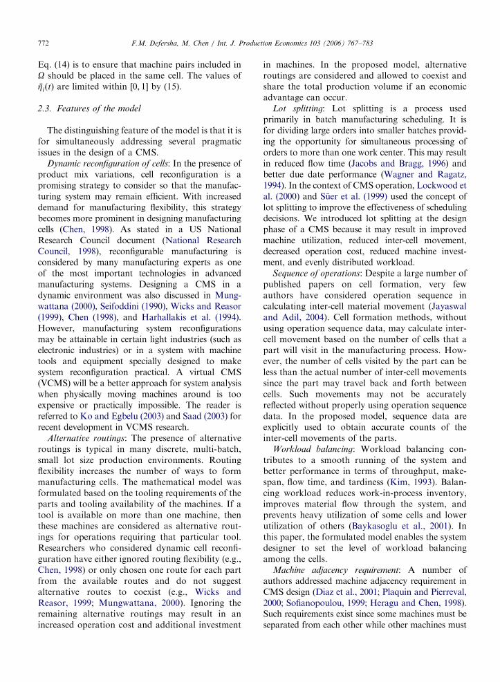
2.3. Features of the model
The distinguishing feature of the model is that it isfor simultaneously addressing several pragmaticissues in the design of a CMS.
Dynamic reconfiguration of cells: In the presence ofproduct mix variations, cell reconfiguration is apromising strategy to consider so that the manufac-turing system may remain efficient. With increaseddemand for manufacturing flexibility, this strategybecomes more prominent in designing manufacturingcells (Chen, 1998). As stated in a US NationalResearch Council document (National ResearchCouncil, 1998), reconfigurable manufacturing isconsidered by many manufacturing experts as oneof the most important technologies in advancedmanufacturing systems. Designing a CMS in adynamic environment was also discussed in Mung-wattana (2000), Seifoddini (1990), Wicks and Reasor(1999), Chen (1998), and Harhallakis et al. (1994).However, manufacturing system reconfigurationsmay be attainable in certain light industries (such aselectronic industries) or in a system with machinetools and equipment specially designed to makesystem reconfiguration practical. A virtual CMS(VCMS) will be a better approach for system analysiswhen physically moving machines around is tooexpensive or practically impossible. The reader isreferred to Ko and Egbelu (2003) and Saad (2003) forrecent development in VCMS research.
Alternative routings: The presence of alternativeroutings is typical in many discrete, multi-batch,small lot size production environments. Routingflexibility increases the number of ways to formmanufacturing cells. The mathematical model wasformulated based on the tooling requirements of theparts and tooling availability of the machines. If atool is available on more than one machine, thenthese machines are considered as alternative rout-ings for operations requiring that particular tool.Researchers who considered dynamic cell reconfi-guration have either ignored routing flexibility (e.g.,Chen, 1998) or only chosen one route for each partfrom the available routes and do not suggestalternative routes to coexist (e.g., Wicks andReasor, 1999; Mungwattana, 2000). Ignoring theremaining alternative routings may result in anincreased operation cost and additional investment
in machines. In the proposed model, alternativeroutings are considered and allowed to coexist andshare the total production volume if an economicadvantage can occur.
Lot splitting: Lot splitting is a process usedprimarily in batch manufacturing scheduling. It isfor dividing large orders into smaller batches provid-ing the opportunity for simultaneous processing oforders to more than one work center. This may resultin reduced flow time (Jacobs and Bragg, 1996) andbetter due date performance (Wagner and Ragatz,1994). In the context of CMS operation, Lockwood etal. (2000) and Suer et al. (1999) used the concept oflot splitting to improve the effectiveness of schedulingdecisions. We introduced lot splitting at the designphase of a CMS because it may result in improvedmachine utilization, reduced inter-cell movement,decreased operation cost, reduced machine invest-ment, and evenly distributed workload.
Sequence of operations: Despite a large number ofpublished papers on cell formation, very fewauthors have considered operation sequence incalculating inter-cell material movement (Jayaswaland Adil, 2004). Cell formation methods, withoutusing operation sequence data, may calculate inter-cell movement based on the number of cells that apart will visit in the manufacturing process. How-ever, the number of cells visited by the part can beless than the actual number of inter-cell movementssince the part may travel back and forth betweencells. Such movements may not be accuratelyreflected without properly using operation sequencedata. In the proposed model, sequence data areexplicitly used to obtain accurate counts of theinter-cell movements of the parts.
Workload balancing: Workload balancing con-tributes to a smooth running of the system andbetter performance in terms of throughput, make-span, flow time, and tardiness (Kim, 1993). Balan-cing workload reduces work-in-process inventory,improves material flow through the system, andprevents heavy utilization of some cells and lowerutilization of others (Baykasoglu et al., 2001). Inthis paper, the formulated model enables the systemdesigner to set the level of workload balancingamong the cells.
Machine adjacency requirement: A number ofauthors addressed machine adjacency requirement inCMS design (Diaz et al., 2001; Plaquin and Pierreval,2000; Sofianopoulou, 1999; Heragu and Chen, 1998).Such requirements exist since some machines must beseparated from each other while other machines must

ARTICLE IN PRESS
Table 3
Number of variables in the linearized model
Variable name Nature of variable Variable count
ZjiklðtÞ Continuous K � L� T �OP
ZiðtÞ Continuous I � T
f þk ðtÞ Continuous K � T
f �k ðtÞ Continuous K � T
nþjil ðtÞ Continuous L� T �OP
n�jil ðtÞ Continuous L� T �OP
Nkl ðtÞ Gen. integer K � L� T
yþkl ðtÞ Gen. integer K � L� T
y�kl ðtÞ Gen. integer K � L� T
rkl ðtÞ Binary K � L� T
pjil ðtÞ Binary L� T �OP
xkðtÞ Binary K � T
bijl ðtÞ Binary L� T �OP
OP: Total number of operations in all of the parts.
Table 4
Number of constraints in the linearized model
Eq. no. Total count
(2) T �OP
(3) K � L� T �OP
(4) L� T �OP
(5) T �OP
(6) K � L� T
(7) K � T
(8) L� T
(9) L� T
(10) K � L� T
(11) K � L� T
(12) K � L� T
(13) NðSÞ � L� T
(14) NðOÞ � L� T
(15) I � T
(17) K � T
(18) K � T
(19) K � T
(21) L� T �OP
(22) L� T �OP
(23) L� T �OP
NðSÞ: Number of machine pairs in S.
NðOÞ: Number of machine pairs in O.
F.M. Defersha, M. Chen / Int. J. Production Economics 103 (2006) 767–783 773
be placed together due to technical and safetyconsiderations. For example, machines that producevibrations, dust, noise, or high temperatures may needto be separated from electronic assembly and finaltesting. In other situations, certain machines should beplaced in the same cells. For example, a heat treatmentstation and a forging station may be placed adjacentto each other for safety reasons. Machines that share acommon resource or those that require a particularoperator’s skill may also be placed in a same cell.
2.4. Linearizing the objective function
The objective function in the model is a non-linear function due to the max function and theabsolute values in the second and third costelements. These terms can be linearized using theprocedures given below.
Linearizing the max function: The max function inthe second cost term can be linearized by introdu-cing non-negative real variables f þk ðtÞ and f �k ðtÞ, anda binary variable xkðtÞ. The term maxf0; ð
PLl¼1
NklðtÞ �PL
l¼1Nklðt� 1ÞÞg can then be replaced byf þk ðtÞ with the following added constraints:
XL
l¼1
NklðtÞ �XL
l¼1
Nklðt� 1Þ
!
¼ f þk ðtÞ � f �k ðtÞ; 8ðk; tÞ, ð17Þ
f þk ðtÞpM � xkðtÞ; 8ðk; tÞ, (18)
f �k ðtÞpM � ð1� xkðtÞÞ; 8ðk; tÞ, (19)
xkðtÞ 2 f0; 1g; 8ðk; tÞ. (20)
Linearizing the absolute value term: The absolutevalue j
PKk¼1Zjþ1;iklðtÞ �
PKk¼1ZjiklðtÞj in the third cost
element of the objective function can be linearizedby introducing non-negative real variables nþijlðtÞ andn�ijlðtÞ, and a binary variable bijlðtÞ. The term thencan be replaced by nþijlðtÞ þ n�ijlðtÞ with followingadded constraints:
XK
k¼1
Zjþ1;iklðtÞ ¼XK
k¼1
ZjiklðtÞ þ nþijlðtÞ � n�ijlðtÞ:
8ði; j; l; tÞ, ð21Þ
nþijlðtÞpM � bijlðtÞ : 8ði; j; l; tÞ, (22)
n�ijlðtÞpM � ð1� bijlðtÞÞ : 8ði; j; l; tÞ, (23)
bijlðtÞ 2 f0; 1g : 8ði; j; l; tÞ. (24)
After these two terms are linearized, the objectivefunction of the integer programming model haslinear terms only. All constraints in the model arealso linear. The number of variables and number ofconstraints in the linearized model are presented inTables 3 and 4, respectively, based on the variableindices.

ARTICLE IN PRESS
Table 5
Data for the part types
Part no. Batch
size Bi
Cost of inter-
cellular
movement per
unit Vi
Demand during
period t
t ¼ 1 t ¼ 2
1 100 6 4000 0
2 150 12 0 3200
3 300 27 4000 2500
4 200 18 0 4500
5 100 15 4400 0
6 100 15 0 4500
7 150 24 0 4500
8 150 12 3600 0
9 150 12 3400 0
10 200 18 6500 0
11 300 24 0 4500
12 100 12 0 3550
13 100 27 2000 6000
14 150 21 4000 0
15 300 27 4400 4500
16 150 24 0 6000
17 200 12 3500 0
18 100 21 3800 5700
19 100 18 4800 0
20 100 12 0 3800
21 100 24 0 3000
22 150 15 4700 3000
23 120 18 5400 0
24 150 27 0 4500
25 150 18 0 4500
F.M. Defersha, M. Chen / Int. J. Production Economics 103 (2006) 767–783774
3. Numerical examples
Several example problems, all solved with LIN-GO, a commercially available optimization soft-ware, are presented in this section. Example 1 isexplained in detail for its input data and computa-tional results. Since, other example problems aresimilar to Example 1, only summarized results arepresented to further illustrate the CMS design issuesaddressed with the proposed model.
3.1. Example 1
In solving this example, we consider 10 differenttypes of machines, 25 part types, and two planningtime periods. The machines are to be grouped intothree relatively independent cells and reconfigura-tion is to be performed at the beginning of thesecond period to respond to the changes ofproduction demand.
3.1.1. Input data and problem size
The input data of this example are given inTables 5–10. In Table 5, data on production batchsize, unit cost of inter-cell movement, and thedemand for the parts in the two time periods aregiven. The tool requirements for the various opera-tions of the parts are given in Table 6. In Table 7,data of tool availability on different machines arepresented. Table 8 contains the data related toalternative routings generated from matching toolrequirement by operations of the parts and toolavailability on the machines. In Table 9 the data formachine overhead costs, operating costs, machineinstallation and removal costs, machine capacities,the maximum number of machines that can beprocured, and machine procurement costs. For thenumerical examples, we assume that machineinstallation cost is the same as machine removalcost. Data for the number of cells to be formed,lower and upper bounds for the cell sizes, list ofmachine pairs that cannot be placed in a same celland workload balancing factor q are given in Table10. To setup a new system at the beginning of thefirst time period, we set
PkNklð0Þ ¼ 0;8l. We
assume that no part processing will be contractedout, so the subcontracting cost Fi was given a largenumber for each part type. Since, the number ofparts in the numerical example is small, thedifferences in the tool consumption cost for a giventool type among the various alternative routes arenegligible and should not influence the choice of the
alternative routes. Hence, tool consumption costswere not considered in this small example problem.
With the data and assumptions, the linearizedmodel has 16,930 variables including 5320 integervariables. The corresponding number of constraintsis 24,030. These counts of variables and constraintscan be reduced by removing variables that can befixed to zero from the model. The variables whichcan be fixed to zero were removed from the modelusing sparse set membership filtering technique ofLINGO (LINDO Systems Inc., 2002). After thesevariables are fixed, some of the constraints becameredundant and were subsequently removed. Theresulting formulation has a total of only 6437variables and 2120 are integer variables. Thenumber of the corresponding constraints wasreduced to 5602.
3.1.2. Solution of Example 1
The cells generated during each time period andthe part assignment to the various cells are given in

ARTICLE IN PRESS
Table 6
Tool requirement of parts
Part no. The index g of the tool required for processing operation j
j ¼ 1 2 3 4 5 6 7 8 9
1 1 10 3 13 15
2 30 31 35 25 27 26 37 36 38
3 6 7 8 2 1 22 24 23
4 16 17 21 36 38
5 34 37 38 26 28 29 27 32 33
6 17 19 21 1 2 37
7 1 2 3 11 12 15 4 5 20
8 6 7 22 23 8 9
9 28 29 33 38 39 34 35
10 16 17 18 20 39 40
11 1 10 12 3 6 24
12 8 9 1 25 24
13 27 26 25 30 31 33 19 18 20
14 22 23 24 17 21
15 3 11 12 5 15 35
16 34 35 25 26 29
17 2 8 9 24
18 10 11 13 1 15
19 18 19 20 36 38 37
20 6 7 8 1 2 9 23 24
21 39 40 27 28 29 22 30 31
22 1 3 10 12 6 24
23 1 2 17 19 21 36
24 22 23 7 6 9
25 28 29 32 34 35 39
Table 7
Tool availability on machines
Machine type k Indices of the available tools
1 1, 2, 3, 4, 5
2 1, 2, 6, 7, 8, 9
3 10, 11, 12, 13
4 12, 13, 14, 15
5 16, 17, 18, 19, 20, 21
6 22, 23, 24
7 25, 26, 27, 28, 29
8 30, 31, 32, 33, 34, 35
9 36, 37, 38, 39, 40
10 36, 37, 38
F.M. Defersha, M. Chen / Int. J. Production Economics 103 (2006) 767–783 775
Tables 11 and 12. Since, the full listing of the valuesof all of the variables ZjiklðtÞ may not be useful, weonly present values of a sample of these variablesfor part types 1, 6, 10, 15 and 21 in Table 13. Part 15is entirely processed in cell 1. This is indicated inTable 11 by a unit value corresponding to the
machines required to process this part. Many otherparts are also processed without inter-cell move-ments. Similar to part 15, part 1 is also processed inone cell during period 1. Notice that the fourthoperation of part 1 is performed partially bymachine type 3 and partially by machine type 4due to alternative routings that coexist. Part 10 isprocessed partially in cell 1 and partially in cell 2due to lot splitting. One can see that part 10 appearsin columns 7 and 10 and there are no values outsidethe diagonal block corresponding to this part.Similar to part 10, part 6 is also processed in twocells during period 2. There is a combined effect oflot splitting and alternative routings as the fourthand fifth operations of this part are performed bymachine type 1 in cell 2 and by machine type 2 incell 3. The first four operations of part 21 areprocessed partially in cell 2 and partially in cell 3.The fifth operation is processed partially in cell 3and partially in cell 1 while the last three operationsare performed within cell 1 only. Hence, there is aninter-cell movement from cell 2 and cell 3 to cell 1.

ARTICLE IN PRESS
Table 8
Routes and alternative routings
Part no. Operation no.
1 2 3 4 5 6 7 8 9
1 (1,100,12) (3,80,18) (1,150,10) (3,120,10) (4,90,16)
(2,110,11) (4,155,8)
2 (8,40,16) (8,40,14) (8,40,16) (7,90,12) (7,120,12) (7,90,10) (9,100,10) (9,130,17) (9,180,16)
(10,120,10) (10,120,18) (10,120,18)
3 (2,90,5) (2,90,10) (2,90,15) (1,100,10) (1,100,16) (6,30,20) (6,40,15) (6,40,10)
(2,120,9) (2,120,15)
4 (5,30,8) (5,30,10) (5,90,12) (9,70,16) (9,70,20)
(10,140,15) (10,120,19)
5 (8,60,9) (9,90,10) (9,60,12) (7,90,6) (7,120,8) (7,100,8) (7,120,10) (8,40,16) (8,60,12)
(10,120,9) (10,120,11)
6 (5,30,16) (5,60,10) (5,90,8) (1,100,12) (1,100,16) (9,100,12)
(2,100,12) (1,120,14) (10,120,12)
7 (1,100,5) (1,100,8) (1,150,6) (3,80,10) (3,120,12) (4,90,14) (1,150,16) (1,150,10) (5,70,8)
(2,120,5) (2,120,9) (4,140,11)
8 (2,90,6) (2,90,8) (6,30,12) (6,40,14) (2,110,8) (2,110,8)
9 (7,120,6) (7,100,12) (8,60,16) (9,60,14) (9,80,20) (8,60,6) (8,60,16)
(10,120,13)
10 (5,30,12) (5,30,6) (5,60,8) (5,70,16) (9,80,7) (9,80,4)
11 (1,100,7) (3,80,10) (3,120,10) (1,150,15) (2,90,8) (6,40,5)
(2,90,7) (4,140,9)
12 (2,110,7) (2,110,11) (1,100,8) (7,90,15) (6,40,15)
(2,120,7)
13 (7,20,5) (7,90,14) (7,90,8) (8,40,10) (8,40,6) (8,60,5) (5,60,10) (5,60,12) (5,70,12)
14 (6,30,16) (6,40,8) (6,40,12) (5,30,6) (5,90,4)
15 (1,150,5) (3,80,10) (3,120,12) (1,150,5) (4,90,8) (8,60,4)
(4,140,11)
16 (8,60,12) (8,60,10) (7,90,14) (7,90,9) (7,100,14)
17 (1,100,16) (2,110,6) (2,110,18) (6,40,12)
(2,120,16)
18 (3,80,5) (3,80,8) (3,130,10) (1,100,8) (4,90,16)
(4,140,9) (2,120,7)
19 (5,60,10) (5,60,9) (5,70,13) (9,70,12) (9,60,12) (9,70,16)
(10,120,11) (10,110,11) (10,120,15)
20 (2,90,8) (2,90,6) (2,110,6) (1,100,9) (1,100,16) (2,110,7) (6,40,15) (6,40,12)
(2,100,9) (2,110,15)
21 (9,80,14) (9,80,10) (7,120,8) (7,120,5) (7,100,5) (6,30,12) (8,40,18) (8,40,12)
22 (1,100,18) (1,150,8) (3,80,14) (3,140,16) (2,90,12) (6,40,12)
(2,105,17) (4,125,15)
23 (1,100,8) (1,110,20) (5,30,7) (5,60,9) (5,90,12) (9,70,12)
(2,120,7) (2,140,18) (10,125,11)
24 (6,30,14) (6,40,16) (2,90,8) (2,90,10) (2,110,8)
25 (7,120,8) (7,120,6) (8,40,12) (8,60,10) (8,60,6) (9,80,5)
Routes and alternative routings were determined by matching the tool requirement of the parts and the tool availability on the machines.
F.M. Defersha, M. Chen / Int. J. Production Economics 103 (2006) 767–783776
This is reflected by elements outside the diagonalblock in Table 12. The reconfiguration performed atthe beginning of period 2 can be found from thedata given in Tables 11 and 12.. For example, sixmachines of type 2, one machine of type 3, and fourmachines of type 6 are added to cell 1 in period 2. Atthe same time, one unit of machine types 1, 4, 7, 8,
9, and 10 as well as two units of machine type 5 areremoved from cell 1 at the beginning of the secondtime period.
3.1.3. Solution analysis for Example 1
Workload balancing: For the generated three cells,the minimum allowable workload is q=L� 100 ¼

ARTICLE IN PRESS
Table 9
Data for machines
Machine type k Hk Ok Ck Iþk I�k QkðtÞ PkðtÞ
t ¼ 1 t ¼ 2 t ¼ 1 t ¼ 2
1 500.00 12.00 2000 75.00 75.00 7 1 12500.00 12700.00
2 600.00 11.00 1800 100.00 100.00 12 1 11800.00 12200.00
3 800.00 8.00 1800 140.00 140.00 10 3 10000.00 10200.00
4 400.00 10.50 2000 90.00 90.00 7 2 11200.00 11200.00
5 900.00 8.50 2000 80.00 80.00 8 4 17200.00 17200.00
6 450.00 10.00 2200 100.00 100.00 9 1 13200.00 13200.00
7 650.00 9.00 1840 70.00 70.00 10 2 16200.00 16200.00
8 450.00 8.00 1800 70.00 70.00 10 1 15000.00 15000.00
9 650.00 13.00 2200 80.00 80.00 10 2 12200.00 12200.00
10 300.00 12.00 2200 75.00 75.00 10 4 13200.00 13200.00
Table 10
Miscellaneous data
Number of cells 3
Lower bound for the cell size 2 machines
Upper bound for the cell size 25 machines
Pair of machines that should not be
located in the same cell (arbitrarily
selected)
{2, 4} and {6, 9}
Pair of machines that should be located in
the same cell (arbitrarily selected)
{1, 3}
Workload balancing factor, q 0.90
F.M. Defersha, M. Chen / Int. J. Production Economics 103 (2006) 767–783 777
0:93� 100 ¼ 30% of the total workload in processing
time with the maximum being ððq=LÞ þ 1� qÞ�
100 ¼ ð0:93þ 1� 0:9Þ � 100 ¼ 40%. In order to see
the impact of enforcing workload balancing, werecalculated the example problem without thisrequirement by letting q ¼ 0. The resulting work-load distributions and the corresponding objectivefunction values are in Table 14. As it can be seenfrom this table, there are significant workloaddifferences among the cells. In period 1, the work-load difference between cell 1 and cell 3 is 569,967processing time in minutes. If we assume theaverage processing time of the operations to be12min, then 47,498 more operations are performedin cell 1 than in cell 3. In period 2, cell 3 receivesonly half of the load of cell 1. Such unbalancedworkload may lead to a poor performance of thesystem in terms of production throughput andincreased work-in-process inventory. For q ¼ 0:9,the workload is evenly distributed among the cellswith 0.5% increment of the objective function value.
Cost savings: Cost savings may come fromdynamic cell reconfiguration, lot splitting, and
routing flexibility. To investigate the cost saving asa result of these features, we solved the model byeliminating these features one at a time. If we addthe constraint:
y�klðtÞ ¼ yþklðtÞ ¼ 0; tX2 (25)
to the basic model, we can enforce that all requiredmachines be installed at the beginning of period 1and no system reconfiguration afterwards. If ZiðtÞ isset to 1 in (5), 8i; t, then no lot-splitting can takeplace. If we add the constraint:
XT
t¼1
XL
l¼1
Z1;1;1;lðtÞ ¼ 0 (26)
to the model, the use of machine type 1 for thefirst operation on part 1 is prevented since thismachine has a higher setup and operation cost thanmachine type 2, i.e., ½ðm1;1;1=B1Þ þO1 � h1;1;1�4½ðm1;1;2=B1Þ þO2 � h1;1;2�. Similar constraints canbe added corresponding to alternative routes. Thuseach operation will have exactly one route andalternative routes will no longer be used in the cellformation decision. Adding the following con-straints to the basic model, the model will selecteither a type 1 machine or a type 2 machine toprocess the first operation of part 1.
XL
l¼1
Z1;1;1;lðtÞpM � X 1ðtÞ, (27)
XL
l¼1
Z1;1;2;lðtÞpM � ð1� X 1ðtÞÞ, (28)
X 1ðtÞ is binary. (29)

ARTICLE IN PRESS
Table 11
Part-cell assignment for period 1
Cell Machine Parts types
Type Qnt. 1 5 9* 10* 23 9* 10* 13* 15 18 19 3 8 13* 14 17 22
C1 M1 2 1 1
M3 1 1
M4 1 1
M5 2 0.33 1
M7 2 1 0.41
M8 2 1 0.41
M9 1 1 0.41 0.33 1
M10 1 1 0.41 1
C1 M1 1 1 1
M3 1 1 1
M4 2 1 1
M5 3 0.67 0.31 1
M7 2 0.59 0.31
M8 1 0.59 0.31 1
M9 1 0.59 0.67 1
M10 2 0.59 1
C3 M1 1 1
M2 6 1 1 1 1
M3 2 1
M5 1 0.69 1
M6 4 1 1 1 1 1
M7 1 0.69
M8 2 0.69
The numbers in the body of the table indicate the proportion of the total demand of parts whose operations are performed in the
corresponding cell.*Parts appearing in more than one column of this table represent spot splitting.
Table 12
Part-cell assignment for period 2
Cell Machine Parts types
Type Qnt. 3 11 12 16* 20 21 6* 7 13* 15 16* 18 2 4 6* 13* 25
C1 M1 1 1 0.94
M2 6 1 1 1 0.94
M3 2 1
M6 4 1 1 1 1
M7 1 1 0.13 1
M8 1 0.13 1
C2 M1 3 0.18 1 1 1
M3 2 1 1 1
M4 3 1 1 1
M5 2 0.18 1 0.66
M7 3 0.60 0.66 0.87
M8 2 0.66 1 0.87
M9 1 0.60 0.18
C3 M2 2 0.06 0.82
M5 1 1 0.82 0.34
M7 3 0.40 1 0.34 1
M8 3 1 0.34 1
M9 3 0.40 1 1 0.82 1
M10 1 1 1
Numbers outside the diagonal blocks indicate the presence of inter-cell movement.
F.M. Defersha, M. Chen / Int. J. Production Economics 103 (2006) 767–783778

ARTICLE IN PRESS
Table 14
Workload distribution
q Cell Workload of cells in processing time and as a percentage of the total workload Objective function value
Period 1 Period 2
0 1 1,527,821 40% 2,053,727 44%
2 1,380,987 36% 1,597,487 34% 2,613,864.00
3 957,854 25% 1,025,005 22%
0.9 1 1,259,986 33% 1,644,312 35%
2 1,160,890 30% 1,616,507 35% 2,626,995.00
3 1,448,759 37% 1,397,494 30%
Table 13
Sample values of ZjiklðtÞ
Period Part no. Cell Machine, ZjiklðtÞ
Operation
1 2 3 4 5 6 7 8
1 15 1 1, 1.00 3, 1.00 4, 1.00 1, 1.00 4, 1.00 8, 1.00
1 1 1 1, 1.00 3, 1.00 1, 1.00 3, 0.90 4, 1.00
4, 0.10
1 10 1 5, 0.33 5, 0.33 5, 0.33 5, 0.33 9, 0.33 9, 0.33
2 5, 0.67 5, 0.67 5, 0.67 5, 0.67 9, 0.67 9, 0.67
2 6 2 5, 0.18 5, 0.18 5, 0.18 1, 0.18 1, 0.18 9, 0.18
3 5, 0.82 5, 0.82 5, 0.82 2, 0.82 2, 0.82 9, 0.82
2 21 2 9, 0.60 9, 0.60 7, 0.60 7, 060
3 9, 0.40 9, 0.40 7, 0.40 7, 040 7, 0.40
1 7, 0.60 6, 1.00 8, 1.00 8, 1.00
Table 15
Cost saving as a result of some features of the model
Feature inhibited from the basic model Objective function value Cost saving by considering the feature
None 2,626,995.00 NA NA
Dynamic reconfiguration of cells 2,661,179.00 34,184.00 1.3%
Lot splitting 2,696,860.00 69,865.00 2.7%
Alternative routings 2,732,050.00 105,055.00 4.0%
Coexistence of alternative routings 2,656,860.00 29,865.00 1.1%
F.M. Defersha, M. Chen / Int. J. Production Economics 103 (2006) 767–783 779
Similar sets of constraints can be added for otherparts and operations having alternative routings.This will prevent the coexistence of alternativeroutings.
By eliminating the features mentioned above oneat a time from the basic model using the corre-
sponding sets of constraints, we recalculated theexample problem to observe the impacts on thesolution of the model. The results are summarizedin Table 15 and cost savings are significant for thisexample problem if dynamic reconfiguration, lotsplitting, and routing flexibility are allowed.
ARTICLE IN PRESS
Table 16
Generic attributes of the 10 additional problems
Problem no. No. of
planning
periods
No. of cells No. of
machines types
No. of part
types
No. of potentially non-zero
variables
No. of
constraints
Integer Total
2 2 3 10 25 2120 6392 5694
3 2 3 10 25 2024 6098 5676
4 2 3 6 25 2040 6190 5376
5 2 3 6 25 1932 5860 5420
6 2 3 6 15 1392 4186 3664
7 2 3 6 15 1392 4186 3772
8 3 3 6 15 2088 6275 5506
9 3 3 6 15 2088 6284 5579
10 2 4 8 20 1856 5474 4928
11 2 4 8 20 5474 1856 4993
Table 17
Impacts of the workload balancing constraint on the workload
distributions and objective function values of the 10 arbitrarily
generated problems
Problem
no.
Maximum cell load difference
as % of total
Objective value
increment (%)
Period q ¼ 0 q ¼ 0:9
F.M. Defersha, M. Chen / Int. J. Production Economics 103 (2006) 767–783780
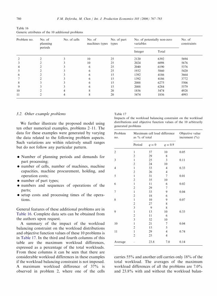
3.2. Other example problems
We further illustrate the proposed model usingten other numerical examples, problems 2–11. Thedata for these examples were generated by varyingthe data related to the following problem aspects.Such variations are within relatively small rangesbut do not follow any particular pattern.
2 1 37 10 0.05
2 29 8
� 3 1 25 3 0.11Number of planning periods and demands forpart processing;
2 24 10
� 4 1 33 4 0.332 26 4
5 1 31 7 0.01
number of cells, number of machines, machinecapacities, machine procurement, holding, andoperation costs;
2 35 10
� number of part types; 6 1 11 6 0.02 �2 29 7
7 1 33 9 0.04
numbers and sequences of operations of theparts;
2 18 6
� 8 1 10 9 0.072 27 8
3 9 8
9 1 13 10 0.33
2 11 6
3 32 10
10 1 21 7 0.04
2 15 5
11 1 29 4 0.74
2 25 4
Average – 23.8 7.0 0.14
setup costs and processing times of the opera-tions.
General features of these additional problems are inTable 16. Complete data sets can be obtained fromthe authors upon request.
A summary of the impact of the workloadbalancing constraint on the workload distributionsand objective function values of these 10 problems isin Table 17. In the third and fourth columns of thistable are the maximum workload differences,expressed as a percentage of the total workloads.From these columns it can be seen that there areconsiderable workload differences in these examplesif the workload balancing constraint is not imposed.A maximum workload difference of 37% isobserved in problem 2, where one of the cells
carries 55% and another cell carries only 18% of thetotal workload. The averages of the maximumworkload differences of all the problems are 7.0%and 23.8% with and without the workload balan-

ARTICLE IN PRESS
Table 18
Cost savings resulted from some features of the model on 10 arbitrarily generated problems
Problem no. Feature eliminated-objective/cost saving
None Dynamic
reconfiguration
Lot splitting Alternative routing Coexistence of
alternative routings
2 3,296,888.00 3,308,990.00 3,661,735.00 3,364,681.00 3,326,555.00
NA 12,102.00 364,847.00 67,793.00 29,667.00
3 3,794,331.00 3,804,331.00 3,879,594.00 3,848,139.00 3,824,084.00
NA 10,000.00 85,263.00 53,808.00 29,753.00
4 2,022,009.00 2,024,922.00 2,065,277.00 2,088,094.00 2,023,695.00
NA 2,913.00 43,268.00 66,085.00 1,686.00
5 2,924,824.00 2,929,882.00 2,986,842.00 3,072,987.00 2,940,365.00
NA 5,058.00 62,018.00 148,163.00 15,541.00
6 1,529,347.00 1,548,218.00 1,548,005.00 1,666,412.00 1,530,340.00
NA 18,871.00 18,658.00 137,065.00 993.00
7 1,535,497.00 1,538,605.00 1,549,114.00 1,705,372.00 1,536,560.00
NA 3,108.00 13,617.00 169,875.00 1,063.00
8 2,067,705.00 2,070,649.00 2,141,568.00 2,283,562.00 2,069,057.00
NA 2,944.00 73,863.00 215,857.00 1,352.00
9 2,214,939.00 2,227,884.00 2,556,638.00 2,246,319.00 2,231,734.00
NA 12,945.00 341,699.00 31,380.00 16,795.00
10 1,744,313.00 1,757,518.00 1,844,063.00 1,769,873.00 1,763,632.00
NA 13,205.00 99,750.00 25,560.00 19,319.00
11 2,439,456.00 2,448,741.00 2,511,847.00 2,478,229.00 2,449,698.00
NA 9,285.00 72,391.00 38,773.00 10,242.00
Average saving in percent 0.50 5.95 6.47 0.53
F.M. Defersha, M. Chen / Int. J. Production Economics 103 (2006) 767–783 781
cing constraint, respectively. The last column of thistable are the increments of the objective functionvalue due to workload balancing constraint. As canbe seen from this column, the increment of theobjective function value is less than 0.1% for theseven of the ten problems and the average percen-tage increment is 0.14%. In Table 18 we present thecost savings observed from these 10 exampleproblems as a result of dynamic reconfiguration,lot splitting, alternative routings and allowingalternative routings to coexist. As can be seen fromthis table, lot splitting and alternative routing haveresulted in significant cost savings with the averagesbeing 5.95% and 6.47%, respectively. Cost savingfrom lot splitting can be due to reduced inter-cellmovement, reduced machine investment, and bettermachine utilization. It can also enable workloadbalancing with minimal inter-cell movement sincethe processing of an operation of a batch can beallocated to different cells. The cost saving from
alternative routings can be from reduced inter-cellmovement, operation cost, setup costs, and machineinvestment cost since it can increase the number ofways in which the cells can be formed to reducethese costs. Dynamic reconfiguration and allowingalternative routings to coexist have resulted inconsiderable cost savings in these 10 problems withthe averages being 0.50% and 0.53%, respectively.
4. Discussion and conclusion
In this paper, a comprehensive mathematicalprogramming model for CMS design is proposed.A commercially available optimization software isused to solve the formulation for small sizeproblems. Computational experience on such smallproblems showed that a significant amount of costsavings can be achieved by considering systemreconfigurations, lot splitting and system flexibility.Our computational results also show that there are

ARTICLE IN PRESSF.M. Defersha, M. Chen / Int. J. Production Economics 103 (2006) 767–783782
significant differences on workload distributionamong the cells, if workload balancing is notattempted. Thus, with this work, we have demon-strated the importance of addressing several designissues in an integrated manner. Since, the proposedmixed integer programming model is NP-hard, weare currently developing heuristic methods toefficiently solve the proposed model for problemsof larger sizes. The heuristic methods will bedesigned to generate several near optimal alterna-tive solutions that will be further evaluated for theirperformances related to machine utilization, work-in-process inventory, and due date.
Acknowledgements
This research is supported by Discovery Grantfrom NSERC of Canada and by Faculty ResearchSupport Fund from the Faculty of Engineering andComputer Science, Concordia University, Mon-treal, Quebec, Canada. The authors sincerely thankthe three anonymous referees for their thoroughreviews of the early versions of this paper and theirvery valuable comments.
References
Akturk, M.S., Turkcan, A., 2000. Cellular manufacturing system
design using a holonistic approach. International Journal of
Production Research 38, 2327–2347.
Askin, R.G., Chiu, K.S., 1990. A graph partitioning procedure
for machine assignment and cell formation in group
technology. International Journal of Production Economics
28, 1555–1572.
Askin, R.J., Vakharia, A.J., 1990. Group technology—cell
formation and operation. In: Cleland, D.I., Bidanda, B.
(Eds.), Automated Factory Handbook: Technology and
Management. TAB Books, Inc., New York, pp. 317–366.
Asokan, P., Prabhakaran, G., Kumar, G.S., 2001. Machine-cell
grouping in cellular manufacturing systems using non-
traditional optimisation techniques—a comparative study.
Integrated Manufacturing Systems 18, 140–147.
Baykasoglu, A., Gindy, N.N.Z., Cobb, R.C., 2001. Capability
based formulation and solution of multiple objective cell
formation problems using simulated annealing. Integrated
Manufacturing Systems 12, 258–274.
Caux, C., Bruniaux, R., Pierreval, H., 2000. Cell formation with
alternative process plans and machine capacity constraints: A
new combined approach. International Journal of Production
Economics 64, 179–284.
Chen, M., 1998. A mathematical programming model for system
reconfiguration in a dynamic cellular manufacturing environ-
ment. Annals of Operations Research 74, 109–128.
Cao, D., Chen, M., 2004. Using penalty function and Tabu
search to solve cell formation problems with fixed cell cost.
Computers and Operations Research 31, 21–37.
Diaz, B.Z., Lozano, S., Racero, J., Gurrero, F., 2001. Machine
cell formation in generalized group technology. Computers
and Industrial Engineering 41, 227–240.
Greene, T., Sadowski, R., 1984. A review of cellular manufactur-
ing assumptions, advantages, and design techniques. Journal
of Operations Management 4, 85–97.
Harhallakis, G., Ioannou, G., Minis, I., Nagi, R., 1994.
Manufacturing cell formation under random product de-
mand. International Journal of Production Research 32,
47–64.
Heragu, S.S., Chen, J.R., 1998. Optimal solution of cellular
manufacturing system design: Benders decomposition ap-
proach. European Journal of Operational Research 107,
175–192.
Jacobs, F.R., Bragg, D.J., 1996. Repetitive lots: Flow time
reduction through sequencing and dynamic batch sizing.
Decision Sciences 19, 281–294.
Jayaswal, S., Adil, G.K., 2004. Efficient algorithm for cell
formation with sequence data, machine replications and
alternative process routings. International Journal of Produc-
tion Research 19, 281–294.
Joines, J., Culbreth, C., King, R., 1996. A comprehensive review
of production oriented cell formation techniques. Interna-
tional Journal of Factory Automation and Information
Management 3, 225–265.
Kim, Y.-D., 1993. A study on surrogate objectives for loading a
certain type of flexible manufacturing system. International
Journal of Production Research 31, 381–392.
Ko, K.-C., Egbelu, P.J., 2003. Virtual cell formation. Interna-
tional Journal of Production Research 41, 2365–2389.
Kusiak, A., 1987. The generalized group technology concept.
International Journal of Production Research 25, 561–569.
LINDO Systems Inc., 2002. LINGO: Users guide. LINDO
Systems Inc., Chicago.
Lockwood, W.T., Mahmoodi, F., Ruben, R.A., Mosier, C.T.,
2000. Scheduling unbalanced cellular manufacturing systems
with lot splitting. International Journal of Production
Research 38, 951–965.
Mansouri, S.A., Husseini, S.M., Newman, S.T., 2000.
A review of the modern approaches to multi-criteria cell
design. International Journal of Production Research 38,
1201–1218.
Mungwattana, A., 2000. Design of cellular manufacturing
systems for dynamic and uncertain production requirements
with presence of routing flexibility. Ph.D. Thesis, Virginia
Polytechnic Institute and State University, Blackburg, VA.
National Research Council, 1998. Visionary manufacturing
challenges for 2020. National Academics Press, Washington,
DC.
Onwubolu, G.C., Mutingi, M., 2001. A genetic algorithm
approach to cellular manufacturing systems. Computers and
Industrial Engineering 39, 125–144.
Plaquin, M.-F., Pierreval, H., 2000. Cell formation using
evolutionary algorithms with certain constraints. Interna-
tional Journal of Production Economics 64, 267–278.
Purcheck, G.F.K., 1974. A mathematical classification as a basis
for the design of group technology production cells. Produc-
tion Engineer 54, 35–48.
Rajamani, D., Singh, N., Aneja, Y., 1990. Integrated design of
cellular manufacturing systems in the presence of alternative
process plans. International Journal of Production Research
30, 1541–1554.

ARTICLE IN PRESSF.M. Defersha, M. Chen / Int. J. Production Economics 103 (2006) 767–783 783
Saad, S.M., 2003. The reconfiguration issues in manufacturing
systems. Journal of Materials Processing Technology 138,
277–283.
Seifoddini, H., 1990. A probabilistic model for machine cell
formation. International Journal of Production Research 9,
69–75.
Selim, H.M., Askin, R.G., Vakharia, A.J., 1998. Cell formation in
group technology: Review, evaluation and direction for future
research. Computers and Industrial Engineering 34, 2–30.
Shafer, S.M., Rogers, D.F., 1991. A goal programming approach
to the cell formation problem. Journal of Operations
Management 10, 28–43.
Shafer, S.M., Kern, G.M., Wei, J.C., 1992. A mathematical
programming approach for dealing with exceptional elements
in cellular manufacturing. International Journal of Produc-
tion Research 30, 1029–1036.
Shtub, A., 1989. Modeling group technology cell formation as a
generalized assignment problem. International Journal of
Production Research 27, 775–782.
Sofianopoulou, S., 1999. Manufacturing cells design with
alternative process plans and/or replicate machines. Interna-
tional Journal of Production Research 37, 707–720.
Solimanpur, M., Vrat, P., Shankar, R., 2004. A multi-objective
genetic algorithm approach to the design of cellular manu-
facturing systems. International Journal of Production
Research 42, 1419–1441.
Su, C.-T., Hsu, C.-M., 1998. Multi-objective machine-part cell
formation through parallel simulated annealing. International
Journal of Production Research 36, 2185–2207.
Suer, G.A., Saiz, M., Gonzalez, W., 1999. Evaluation of
manufacturing cell loading rules for independent cells.
International Journal of Production Research 36,
2185–2207.
Wagner, B.J., Ragatz, G.L., 1994. The impact of lot splitting on
due date performance. Journal of Operations Management
12, 13–25.
Wei, J.C., Gaither, N., 1990. A capacity constrained multi-
objective cell formation method. Journal of Manufacturing
Systems 9, 222–232.
Wemmerlov, U., Hyer, N.L., 1986. Procedures for part-
family/machine group identification problem in cellular
manufacturing. Journal of Operations Management 6,
125–145.
Wemmerlov, U., Johnson, D.J., 1997. Cellular manufacturing at
46 user plants: Implementation experiences and performance
improvements. International Journal of Production Research
35, 29–49.
Wicks, E.M., Reasor, R.J., 1999. Designing cellular manufactur-
ing systems with dynamic part populations. IIE Transactions
31, 11–20.
Xambre, A.R., Vilarinho, P.M., 2003. A simulated annealing
approach for manufacturing cell formation with multiple
identical machines. European Journal of Operational Re-
search 151, 434–446.
Zhao, C., Zhiming, W., 2000. A genetic algorithm for manu-
facturing cell formation with multiple routes and multiple
objectives. International Journal of Production Research 38,
385–395.