a computational platform for gene expression analysis · a computational platform for gene...
TRANSCRIPT

FACULDADE DE ENGENHARIA DA UNIVERSIDADE DO PORTO
A Computational Platform for Gene
Expression Analysis
Diogo André Rocha Teixeira
Mestrado Integrado em Engenharia Informática e Computação
Supervisor: Rui Camacho
Second Supervisor: Nuno Fonseca (EMBL-EBI, Cambridge, UK)
July 19, 2014


A Computational Platform for Gene ExpressionAnalysis
Diogo André Rocha Teixeira
Mestrado Integrado em Engenharia Informática e Computação
Approved in oral examination by the committee:
Chair: Ana PaivaExternal Examiner: Sérgio Matos
Supervisor: Rui Camacho
July 19, 2014


Abstract
The advent of next generation sequencing methods has revolutionized the field of molecularbiology in the past few years. Nowadays, we are able to produce enormous amounts of bio-logical information, both quickly and at low cost. As such, tools have to evolve accordingly,in order to cope with such large volumes of information. In this report we discuss the usageof computer tools capable of conducting gene expression profiling based on information ob-tained through RNA Sequencing techniques, applied to a specific set of biological problems.In particular, we present the idealization process and implementation details of a web plat-form capable of addressing these problems, as well as the actual platform prototype. Theprototype’s functionality is showcased with a real case study, produced in collaboration withbiology researchers. This report also includes a literature review, covering both the biologicaland technical aspects of the work, with special emphasis in machine learning techniques ap-plied to data mining tasks. Lastly, we review the work done and results obtained so far andoutline the possible future of the web platform.
i

ii
Resumo
O advento das técnicas de sequenciação de nova geração revolucionou o campo da biologiamolecular nos últimos anos. Hoje em dia somos capazes de produzir enormes quantidadesde informação biológica rapidamente e a baixo custo. Assim sendo, as ferramentas devemtambém evoluir, a fim de lidarem com estas extensas quantidades de informação. Neste re-latório discutimos o uso de ferramentas informáticas capazes de analisar perfis de expressãogénica com base em informação obtida através de técnicas de RNA Sequencing, aplicadas aum conjunto específico de problemas biológicos. Em particular, apresentamos o processo deidealização e os detalhes de implementação de uma plataforma web capaz de resolver estesproblemas, assim como o protótipo funcional dessa plataforma. As funcionalidades deste pro-tótipo são demonstradas através de um caso de estudo real, produzido em colaboração cominvestigadores da área da biologia. Este relatório inclui também uma revisão da literatura, co-brindo os aspetos biológicos e técnicos deste trabalho, com um ênfase especial em técnicas deaprendizagem máquina aplicadas a tarefas de data mining. Por fim, revemos todo o trabalhoefetuado e os resultados obtidos até ao momento e delineamos as possibilidades futuras paraa plataforma web.
iii

iv

Acknowledgements
First of all, I would like to direct my gratitude to my supervisor, Rui Camacho (FEUP). Hisconcern about my work and the helpfulness he has always shown were key factors for thesuccess of this project. I extend the same gratitude to my co-supervisor, Nuno Fonseca (EMBL-EBI), for his endless patience in answering my questions.
I would also like thank Alexandra Moreira, Andrea Cruz and Jaime Freitas (IBMC) for thefantastic way they always welcomed me. Their willingness to help me through the difficult oflearning a completely new field of study was fundamental to my progress.
A very special thank you to my all my friends at FEUP, that were with me in what is surelyone of the best periods in my life. In particular I would like to acknowledge Pedro. Ourconstant competition, along with our shared antics, made working on this project that muchmore fun and fulfilling.
To my parents, Joaquim and Maria, I leave a truly heartfelt thank you; for all the nightsthey spent awake worrying about me; for all their guidance and wisdom; for being with me inevery good and bad moment of my life. I would not be the person I am today without them.
Lastly, but definitely not least, I thank my girlfriend, Raquel. Of everything I have and oweto her, nothing is more important than the smile she puts on my face every day, as she givesme the strength to face the world.
Diogo Teixeira
v

vi

“ Often people, especially computer engineers, focus on the ma-chines. They think, "By doing this, the machine will run faster. Bydoing this, the machine will run more effectively. By doing this, themachine will something something something." They are focusingon machines. But in fact we need to focus on humans, on how hu-mans care about doing programming or operating the applicationof the machines. We are the masters. They are the slaves. ”
Yukihiro Matsumoto
vii

viii

Contents
1 Introduction 11.1 Domain Problem . . . . . . . . . . . . . . . . . . . . . . . . . . . . . . . . . . . . . . . . 11.2 Motivation and Objectives . . . . . . . . . . . . . . . . . . . . . . . . . . . . . . . . . . 21.3 Project . . . . . . . . . . . . . . . . . . . . . . . . . . . . . . . . . . . . . . . . . . . . . . 31.4 Structure of the Report . . . . . . . . . . . . . . . . . . . . . . . . . . . . . . . . . . . . 3
2 Problem Domain and Technological Base Concepts 52.1 Biological Base Concepts . . . . . . . . . . . . . . . . . . . . . . . . . . . . . . . . . . . 5
2.1.1 Gene Expression . . . . . . . . . . . . . . . . . . . . . . . . . . . . . . . . . . . 52.1.2 RNA-Binding Proteins . . . . . . . . . . . . . . . . . . . . . . . . . . . . . . . . 62.1.3 Sequencing . . . . . . . . . . . . . . . . . . . . . . . . . . . . . . . . . . . . . . 72.1.4 Transcriptome Assembly . . . . . . . . . . . . . . . . . . . . . . . . . . . . . . 82.1.5 Relevant Standard File Formats . . . . . . . . . . . . . . . . . . . . . . . . . . 8
2.2 RNA-Seq Analysis . . . . . . . . . . . . . . . . . . . . . . . . . . . . . . . . . . . . . . . 102.2.1 RNA-Seq Pipeline . . . . . . . . . . . . . . . . . . . . . . . . . . . . . . . . . . 102.2.2 RNA Sequencing, Read Alignment and Analysis Tools . . . . . . . . . . . . 132.2.3 Differential Expression Analysis Tools . . . . . . . . . . . . . . . . . . . . . . 142.2.4 File Manipulation and Pre-processing Tools . . . . . . . . . . . . . . . . . . 15
2.3 Data Mining . . . . . . . . . . . . . . . . . . . . . . . . . . . . . . . . . . . . . . . . . . 162.3.1 Clustering Techniques . . . . . . . . . . . . . . . . . . . . . . . . . . . . . . . . 172.3.2 Clustering Algorithms . . . . . . . . . . . . . . . . . . . . . . . . . . . . . . . . 192.3.3 Clustering Evaluation and Assessment . . . . . . . . . . . . . . . . . . . . . . 212.3.4 Common Distance Measures . . . . . . . . . . . . . . . . . . . . . . . . . . . . 222.3.5 Clustering Tools . . . . . . . . . . . . . . . . . . . . . . . . . . . . . . . . . . . 25
2.4 Chapter Conclusions . . . . . . . . . . . . . . . . . . . . . . . . . . . . . . . . . . . . . 27
3 Solution Description 293.1 Overview . . . . . . . . . . . . . . . . . . . . . . . . . . . . . . . . . . . . . . . . . . . . 293.2 Gene Expression Analysis Pipeline . . . . . . . . . . . . . . . . . . . . . . . . . . . . . 30
3.2.1 Analysis Configuration . . . . . . . . . . . . . . . . . . . . . . . . . . . . . . . 303.2.2 Experimental Data Management . . . . . . . . . . . . . . . . . . . . . . . . . 303.2.3 Analysis Workflow . . . . . . . . . . . . . . . . . . . . . . . . . . . . . . . . . . 30
3.3 RNA Binding Protein Analysis Web Platform . . . . . . . . . . . . . . . . . . . . . . . 323.3.1 Experimental Data . . . . . . . . . . . . . . . . . . . . . . . . . . . . . . . . . . 323.3.2 User Information Management . . . . . . . . . . . . . . . . . . . . . . . . . . 333.3.3 Analysis Workflow . . . . . . . . . . . . . . . . . . . . . . . . . . . . . . . . . . 33
3.4 Tool Integration . . . . . . . . . . . . . . . . . . . . . . . . . . . . . . . . . . . . . . . . 343.5 Chapter Conclusions . . . . . . . . . . . . . . . . . . . . . . . . . . . . . . . . . . . . . 34
ix

CONTENTS
4 Implementation 354.1 Gene Expression Analysis Pipeline . . . . . . . . . . . . . . . . . . . . . . . . . . . . . 35
4.1.1 Combining Differential Expression Results . . . . . . . . . . . . . . . . . . . 354.2 RNA Binding Protein Analysis Web Platform . . . . . . . . . . . . . . . . . . . . . . . 36
4.2.1 Web Interface . . . . . . . . . . . . . . . . . . . . . . . . . . . . . . . . . . . . . 364.2.2 Data Persistance . . . . . . . . . . . . . . . . . . . . . . . . . . . . . . . . . . . 364.2.3 Analysis Server . . . . . . . . . . . . . . . . . . . . . . . . . . . . . . . . . . . . 364.2.4 Analysis Workflow . . . . . . . . . . . . . . . . . . . . . . . . . . . . . . . . . . 374.2.5 Base Analysis . . . . . . . . . . . . . . . . . . . . . . . . . . . . . . . . . . . . . 374.2.6 Data Set Enrichment . . . . . . . . . . . . . . . . . . . . . . . . . . . . . . . . 404.2.7 Clustering Analysis . . . . . . . . . . . . . . . . . . . . . . . . . . . . . . . . . . 414.2.8 Web Interface . . . . . . . . . . . . . . . . . . . . . . . . . . . . . . . . . . . . . 43
4.3 Chapter Conclusions . . . . . . . . . . . . . . . . . . . . . . . . . . . . . . . . . . . . . 46
5 Case Studies 475.1 Gene Expression Analysis Pipeline . . . . . . . . . . . . . . . . . . . . . . . . . . . . . 47
5.1.1 Case Study Setup . . . . . . . . . . . . . . . . . . . . . . . . . . . . . . . . . . . 475.1.2 Comparison with Previous Results . . . . . . . . . . . . . . . . . . . . . . . . 49
5.2 RNA Binding Protein Analysis Web Platform . . . . . . . . . . . . . . . . . . . . . . . 495.2.1 Case Study Setup . . . . . . . . . . . . . . . . . . . . . . . . . . . . . . . . . . . 505.2.2 Results . . . . . . . . . . . . . . . . . . . . . . . . . . . . . . . . . . . . . . . . . 515.2.3 Correctness and Completeness of the Results . . . . . . . . . . . . . . . . . . 535.2.4 Comparison with Previous Method . . . . . . . . . . . . . . . . . . . . . . . . 54
5.3 Chapter Conclusions . . . . . . . . . . . . . . . . . . . . . . . . . . . . . . . . . . . . . 56
6 Conclusions 576.1 Objective Fulfilment . . . . . . . . . . . . . . . . . . . . . . . . . . . . . . . . . . . . . 576.2 Future Work . . . . . . . . . . . . . . . . . . . . . . . . . . . . . . . . . . . . . . . . . . 58
References 59
Glossary 62
A iRAP Example Configuration 67
B Examples of Biological Information Files 71B.1 SAM Example . . . . . . . . . . . . . . . . . . . . . . . . . . . . . . . . . . . . . . . . . 71B.2 VCF Example . . . . . . . . . . . . . . . . . . . . . . . . . . . . . . . . . . . . . . . . . . 72B.3 FASTQ Example . . . . . . . . . . . . . . . . . . . . . . . . . . . . . . . . . . . . . . . . 72B.4 FASTA Example . . . . . . . . . . . . . . . . . . . . . . . . . . . . . . . . . . . . . . . . 73B.5 GTF/GFF Example . . . . . . . . . . . . . . . . . . . . . . . . . . . . . . . . . . . . . . 73
x

List of Figures
2.1 Overall structure of a gene . . . . . . . . . . . . . . . . . . . . . . . . . . . . . . . . . 62.2 Removal of introns from precursor mRNA . . . . . . . . . . . . . . . . . . . . . . . . 62.3 Role of RBPs in the RNA metabolism process . . . . . . . . . . . . . . . . . . . . . . 72.4 Representation of a standard RNA-Seq analysis pipeline . . . . . . . . . . . . . . . 122.5 iRAP RNA-Seq data analysis pipeline . . . . . . . . . . . . . . . . . . . . . . . . . . . 132.6 Example of a silhouette plot . . . . . . . . . . . . . . . . . . . . . . . . . . . . . . . . 232.7 RapidMiner user interface . . . . . . . . . . . . . . . . . . . . . . . . . . . . . . . . . . 262.8 Weka interface selection . . . . . . . . . . . . . . . . . . . . . . . . . . . . . . . . . . . 26
3.1 Gene expression analysis pipeline workflow . . . . . . . . . . . . . . . . . . . . . . . 313.2 Simplified PBS Finder workflow . . . . . . . . . . . . . . . . . . . . . . . . . . . . . . 33
4.1 PBS Finder workflow . . . . . . . . . . . . . . . . . . . . . . . . . . . . . . . . . . . . . 384.2 Job view example . . . . . . . . . . . . . . . . . . . . . . . . . . . . . . . . . . . . . . . 444.3 Transcript view example . . . . . . . . . . . . . . . . . . . . . . . . . . . . . . . . . . . 454.4 Protein view example . . . . . . . . . . . . . . . . . . . . . . . . . . . . . . . . . . . . . 46
5.1 Comparison between manual RBP analysis and automatic RBP analysis . . . . . . 55
xi

LIST OF FIGURES
xii

List of Tables
3.1 Examples of identifiers accepted by PBS Finder . . . . . . . . . . . . . . . . . . . . . 32
4.1 Information retrieved for genes and transcripts in the base analysis stage . . . . . 394.2 Information retrieved for proteins in the data set enrichment stage . . . . . . . . 40
5.1 Specifications of the test environment used for the case study experiments . . . . 485.2 Number of distinct lines resulting from differential expression analysis . . . . . . 495.3 RhoGTPase family genes used as data set in the case study . . . . . . . . . . . . . . 505.4 Specifications of the test environments used for the case study experiments . . . 515.5 Case study results generated by PBS Finder . . . . . . . . . . . . . . . . . . . . . . . 525.6 RBPs found to characterize each cluster . . . . . . . . . . . . . . . . . . . . . . . . . 535.7 Execution times of the case study data set in two different environments . . . . . 565.8 Results comparison between manual analysis and both test machines . . . . . . . 56
xiii

LIST OF TABLES
xiv

List of Algorithms
2.1 Partitioning Around Medoids (PAM) algorithm . . . . . . . . . . . . . . . . . . . . . . 20
3.1 Combination of differential expression results . . . . . . . . . . . . . . . . . . . . . . 32
4.1 Processing a new analysis request from the web interface . . . . . . . . . . . . . . . 374.2 Selection of best clustering results . . . . . . . . . . . . . . . . . . . . . . . . . . . . . 42
xv

LIST OF ALGORITHMS
xvi

Abbreviations
k-NN k-Nearest-Neighbors.
API Application Programming Interface.
BLAST Basic Local Alignment Search Tool.
cDNA Complementary DNA.
CPU Central Processing Unit.
CSS Cascading Style Sheets.
DBMS DataBase Management System.
DNA DeoxyriboNucleic Acid.
ENA European Nucleotide Archive.
GUI Graphical User Interface.
HTML HyperText Markup Language.
IBMC Instituto de Biologia Molecular e Celular.
ILP Inductive Logic Programming.
mRNA Messenger RNA.
NCBI National Center for Biotechnology Information.
NGS Next Generation Sequencing.
PAM Partition Around Medoids.
RBP RNA Binding Protein.
RNA Ribonucleic Acid.
rRNA Ribosomal RNA.
SAM Sequence Alignment/Map.
xvii

SQL Structured Query Language.
SRA Sequence Read Archive.
tRNA Transfer RNA.
WTSS Whole Transcriptome Shotgun Sequencing.

Chapter 1
Introduction
Molecular biology is a branch of biology that studies biological activities of living beings, at
a molecular level. The grounds for this field of study were set in the early 1930s, although
it only emerged in its modern form in the 1960s, with the discovery of the structure of DNA.
Among the processes studied by this branch of biology is gene expression. Gene expression
(further explained in Chapter 2) is the process by which DNA molecules are transformed
into useful genetic products, typically proteins, which are essential for living organisms. This
knowledge is not only important in fields like evolutionary or molecular biology, but has
crucial applications in fields such as medicine. One example of such an application is the
usage of gene expression analysis in the diagnosis and treatment of cancer patients [PASH03].
With the advent of NGS (Next Generation Sequencing) techniques, researchers have at
their disposal huge amounts of sequencing data, that is not only cheap and fast to produce,
but also commonly available. This data can then be used to obtain relevant information
about organisms’ gene expression. But, as the cost of sequencing genomes was reduced, the
cost of processing such information was increased. NGS techniques tend to produce much
smaller reads1 than previously used techniques, presenting a more challenging problem, from
a computational standpoint [Wol13].
1.1 Domain Problem
Despite its great advancements in the past decades, molecular biology is still a relatively
new subject and, as such, there are still a lot of unknowns and partial knowledge in this
area. In respect to gene expression, some mechanisms of this intricate process are yet to
be fully understood. One such mechanism is the one that regulates the transcription speed
of RNA. One of the objectives of this thesis is to understand how the final sequences of a
gene’s exons are responsible for the speed at which the exons themselves are transcribed. The
1A read is a single fragment of a genome/transcriptome, obtained through sequencing techniques.
1

Introduction
other objective is to understand how RNA-Binding Protein (RBP) manipulation can be used to
better understand an organism’s gene expression. These are, however, complex tasks that can
be further decomposed in the three main problems that were addressed in the thesis, namely:
• Sequencing read alignment against a reference genome and differential expression anal-
ysis between samples of different individuals (of the same species). This is effectively
one of the most complex problems addressed in the thesis. We used data obtained
through a sequencing method called RNA Sequencing2. Further insight about this
method will be given in Chapter 2, with particular emphasis on tools used to align
and analyze this data (Section 2.2.2).
• Gene enrichment and RBP analysis. This part of the work aims to collect as much rele-
vant information as possible about the particular genes being studied at the time, to help
biologists better understand their function. RBP knowledge is particularly important for
gene manipulation and a very useful tool for better understanding gene expression, as
further described in Chapter 2.
• Further analysis of the produced data, using machine learning techniques for data min-
ing, specifically for clustering analysis. These techniques were employed in an effort to
give biologists more relevant information about gene expression, uncovering possible
relationships in the retrieved information. This topic will be developed in Section 2.3.
Solving these problems requires the use of computational tools. As such, the development
of a computer system (or multiple systems) to tackle these problems emerges as another
objective of the thesis. The details of the design of this system will be presented in Chapter 3,
while its concrete implementation will be discussed in Chapter 4.
1.2 Motivation and Objectives
Gene expression analysis is essential for modern day molecular biology. Among many of the
possible applications of this information, we can highlight: better classification and diagnosis
of diseases, assessing how cells react to a specific treatment, and others.
While nowadays powerful computational tools exist to target almost any biology problem,
many of those tools require a very specific set of technical skills and have a steep learning
curve. Possibly the most important motivation behind this thesis, and ultimately its main
objective, is to provide researchers with powerful yet simple and user friendly tools. This
means developing a system simple enough that any user can learn to operate in a short period
of time with minimal effort, but sufficiently advanced to suit the user’s research needs.
Another typical problem that biology researchers face nowadays is information dispersion
and the repetitive and lengthy task of compiling that information. Researchers frequently
2RNA Sequencing is also referred to as Whole Transcriptome Shotgun Sequencing, or WTSS.
2
Introduction
have to manually merge information originating from a multitude of platforms, which use
inconsistent formats and notations. Our objective is therefore to provide a system that is able
to take this burden off the user, making the process faster and simpler.
1.3 Project
The project itself revolves around the development of a prototype computer system, capable
of solving the aforementioned problems. Due to the complexity of the complete system, its de-
velopment followed a modular organization (further described in Chapter 3). The envisioned
system architecture is divided into three major components:
Differential expression analysis pipeline is responsible for aligning reads against a refer-
ence genome and compare contrasts between different samples. The pipeline is based
on the preexisting iRAP pipeline3. The pipeline’s capabilities are further enhanced with
both job configuration automation and consolidation of differential expression results
from multiple tools.
RNA-binding protein analysis workflow aggregates information about RBPs from multiple
biologic web databases (Ensembl, NCBI, UniProt, etc.) and organizes it in ways that
are useful to biology researchers. Moreover, this information is clustered using data
mining techniques, in order to reveal groups of genes and RBPs that may hold biologic
relevance.
Web platform is responsible for storing and managing genetic data, coordinating interaction
between the other components of the system and providing a web interface for user
interaction. This component is based mainly on typical web technologies, that is, a
document based database for data storage (MongoDB), a web framework for business
logic implementation (Padrino) and web markup and styling languages for interface
implementation (HTML, CSS).
1.4 Structure of the Report
Besides the introduction chapter, this document is composed by five additional chapters.
Chapter 2 introduces some basic biology and RNA-Seq concepts, that are essential to un-
derstand the problems with which this document deals. Furthermore, we describe the main
techniques used for genome/transcriptome sequencing and assembly, their differences, appli-
cations and the tools and data formats typically used in those areas. Lastly, we give some
insight about data mining algorithms and how they will be applied in the context of the
project. Chapter 3 presents the design of the software solution. The basic system architecture
is outlined in this chapter, as well as relevant design decisions. Chapter 4 establishes relevant
3https://code.google.com/p/irap/
3

Introduction
implementation details for the developed solution, giving a more in depth knowledge about
its inner workings. Used technologies are also reviewed, and their selection is justified. In
Chapter 5 we present the case study that was used to assess the quality of the produced so-
lutions. We review the test data set, test conditions and obtained results. Lastly, Chapter 6
sums up what was accomplished during the project. We review our objectives in terms of their
fulfilment and present some possibilities for future work.
4

Chapter 2
Problem Domain and Technological
Base Concepts
In this chapter we begin by making a more in-depth presentation of the process of gene
expression. This will be followed by a literature and state-of-the-art review in the fields of read
alignment, differential expression analysis and data mining. We will present the tools used in
the development of the analysis pipelines and the web platform. Lastly, we review some results
evaluation techniques and relevant data representation formats for genetic information.
2.1 Biological Base Concepts
Before dwelling in the details of the state of the art that constitute the foundations of the
thesis, it is important to explain some concepts of the domain of molecular biology.
2.1.1 Gene Expression
As explained in Chapter 1, gene expression is the mechanism by which an organism’s DNA
can be expressed into functional genetic products, like proteins. This process starts with the
genetic code, or nucleotide sequence, of each gene. Different genes in an organism’s DNA
are responsible for the creation of different genetic products. The process of gene expression
itself is composed by two main stages, transcription and translation [GEN].
Transcription is the stage at which genetic data in the form of DNA is used to synthesize
RNA, being this the process that concerns the thesis’ main question. Several different types
of RNA are produced by this process, including messenger RNA (which specifies the sequences
of amino acids that form a protein), ribossomal RNA and transfer RNA, both later used in the
translation stage. Simplifying a gene’s structure, it can be seen as composed by two types of
sequences, introns and exons, as seen in Figure 2.1.
5

Problem Domain and Technological Base Concepts
Exon 1 Exon 2 Exon 3 Exon 4Intron 1 Intron 2 Intron 3
Gene
DNA
Figure 2.1: Overall structure of a gene, with its different areas (simplified).
The exons are useful in the gene expression process, being also known as coding regions.
Introns, on the other hand, are not used in the process. They are present in an early stage
mRNA molecule, the precursor mRNA, but are later removed (or spliced) in the final molecule
before the translation stage [GEN]. Figure 2.2 illustrates the removal of introns from the
mRNA molecule, during the splicing process.
Exon 1 Exon 2 Exon 3Intron 1 Intron 2
5′ 3′
Exon 1 Exon 2 Exon 35′ 3′
Precursor mRNA
Mature mRNA
splicing
Figure 2.2: The removal (splicing) of introns from the precursor mRNA, during the transcrip-tion process.
After the conclusion of the transcription process comes the translation process. In this
process, the synthesized mRNA is used to specify the sequence of amino acids that constitute
the particular protein being produced. The other types of RNA molecules (rRNA and tRNA)
are also used in this stage of the gene expression process.
2.1.2 RNA-Binding Proteins
RNA-binding proteins, also referred to as RBP, regulate every aspect of the RNA metabolism,
including pre-mRNA splicing, mRNA transport, location, stability and translation control
6

Problem Domain and Technological Base Concepts
[CWD09, MMNMMN13, SH07, SH09], as shown in Figure 2.3.
Cell
Nucleus
Gene
1. Splicing
2. Transport
Cytoplasm
Protein
5. Translation Control
3. Localization4. Stability
Figure 2.3: Diagram of a typical cell showing the multiple roles of RBPs in post transcriptionalprocesses [JM11]. The grey ellipses represent RBPs. The numbered text represents the dif-ferent processes in which RBPs take part. Multiple RBPs can bind with a single RNA at oneor more locations, creating an abundance of different combinations and possibilities in everystep of the RNA metabolism.
The binding of RBPs to RNA depends on different RNA-sequence specificities and affinities.
This aspect, coupled with the existence of hundreds of RBPs in an organism, gives rise to a
plethora of different combinations and outcomes to the RNA metabolism.
RBPs regulate gene expression in health and disease, and mutations affecting the function
of RBPs may cause several diseases [CWD09]. Therefore, understanding the binding patterns
of RBPs during a particular biological process is crucial to get insight into that process, both
during health and disease conditions.
2.1.3 Sequencing
Obtaining genetic information is done experimentally, by employing a sequencing technique.
For quite some time this process was carried out using Sanger’s and other similar sequencing
methods [RF09]. Though effective, such methods were notably slow and costly, with large
projects like the Human Genome Project (HGP) consuming roughly thirteen years and US$ 3
7

Problem Domain and Technological Base Concepts
billion. These limitations were so severe that, other than the realm of human genetics, this
kind of study was restricted to model organisms, such as the fruit fly and mouse genomes
[Wol13]. The past few years have seen the appearance and rise in popularity of the NGS tech-
niques. These techniques differ from the more classical ones by producing larger amounts of
information, at lower cost. As such, the techniques can be easily employed by single labora-
tories, which has greatly contributed to their popularity.
The rise in popularity and availability of NGS techniques, coupled with the importance
of RNA knowledge in understanding gene expression, led to the appearance of RNA-Seq.
RNA-Seq makes use of these newly available deep-sequencing techniques to profile complete
transcriptomes. This is, however, a difficult task to accomplish. NGS techniques produce
shorter reads than their older counterparts, being that “(...) transcriptome assembly from
billions of RNA-Seq reads (...) poses a significant informatics challenge” [MW11, p. 671].
Although this thesis does not deal with the problems of sequencing techniques, it is im-
portant to indicate that the read data sets that were used resulted from NGS techniques, in
particular RNA-Seq. As such, suitable tools for this particular type of data were used.
2.1.4 Transcriptome Assembly
Transcriptome assembly is the process by which experimentally obtained RNA data reads can
be organized and merged together in a partial or complete transcriptome. As stated above, the
advent of next generation sequencing techniques, with their reduced costs, greatly increased
the availability of transcript sequencing data.
For years, microarrays were the standard tool available for examining features of the
transcriptome and global patterns of gene expression [Wol13]. However, microarrays are
typically more oriented towards assembly against existing reference data, hence limiting their
application to species with well known reference genomes. This is a severe constraint, as NGS
techniques allow to cheaply obtain genetic information of previously non-studied species. This
is one of the reasons that led to the inception of RNA-Seq. Contrary to microarrays, RNA-Seq
techniques are able to wield results that are suitable for both reference guided assembly and
de novo assembly approaches [WL09]. De novo or exploratory assembly has captured the
interest of researchers in the past few years, leading to the appearance of multiple RNA-Seq
tools that are capable of making this type of assembly without a reference genome [FEB+11].
Transcriptome assembly was not performed during this thesis, as its main focus in terms of
the RNA-Seq process is read alignment and differential expression analysis.
2.1.5 Relevant Standard File Formats
As expected, the great diversity of RNA-Seq tools brings with it a wealth of file formats. Some
of these formats are developed from the ground up to satisfy a specific need, while others are
mere contextual adaptations or specializations of already established formats. Below we will
present a few of the most popular and widely spread file formats, talking about their basic
8

Problem Domain and Technological Base Concepts
structure, the types of data they represent and their applications. Some examples of these file
formats can be consulted in Appendix B.
FASTA
FASTA is the standard line and character sequence format used by NCBI [NCB], using this
organization’s character code conventions (see Appendix B.4). It is a simple format, that can
be used to easily store data represented by character sequences, like nucleotide (DNA, RNA)
or amino acid (protein) sequences. This file format is widely use to store sequencing reads,
DNA/RNA sequences and other character sequences in database systems. Its simplicity makes
it extremely easy to manipulate and parse, presenting itself as an attractive solution for data
transfer between different tools.
FASTQ
FASTQ is used to store character sequences, typically nucleotide sequences [CFG+10] (see
Appendix B.3). It is quite similar to the standard FASTA format, in respect to the manner in
which character sequences are represented. However, for every sequence, there is a second
sequence of equal length, representing the quality scores of the original sequence. These
quality scores are also represented as single characters, taking values between ASCII-33 and
ASCII-126. It is typically used in the same situations as the FASTA format, when quality scores
are available/relevant.
SAM and BAM
The SAM format is a text format for storing sequence alignment data [Lab] (see Appendix
B.1). It is widely used to store mapping information between sequencing reads and a given
reference genome. This sort of information is typically the product of sequencing alignment
tools, that consume sequencing reads from FASTQ files and align them with a reference
genome.
The BAM format contains exactly the same information as the SAM format and the same
rules apply for both formats. The difference between both formats lies in their encoding.
While SAM is a text based format, BAM is a binary format. This means that BAM sacrifices
human readability for increased machine processing performance, as it is more efficient to
work with compressed and indexed binary data.
VCF
VCF is a text file format used to store gene sequence variants [Smi13] (see Appendix B.2). In
the past few years, as larger and larger genome sequencing projects became more common
9

Problem Domain and Technological Base Concepts
(like the 1000 Genomes Project1), storing such large amounts of information became a serious
concern. Instead of storing the complete genome, VCF stores only the variations (and their
respective positions) of newly sequenced genomes relatively to a known reference genome,
typically in a compressed text file. As such, it is a format often used when building genome
databases.
GFF and GTF
GFF is a text based file format to store gene features [San11] (see Appendix B.5). Many
genome assembly tools execute this process in two separate steps: feature detection for iden-
tification of specific regions (exons, introns, etc.) and genome assembly, using those features
as reference. However, it is beneficial to decouple these two steps, using different and more
efficient tools for each. As such, the GFF format emerged as a protocol for feature information
transfer between tools.
The GTF format is similar to the GFF format, in which it is based. It is also used in similar
situations. However, GTF builds on top of GFF, defining additional conventions, specific to
the domain of genetic information. Despite their initial relation, both formats continue to be
developed individually.
2.2 RNA-Seq Analysis
2.2.1 RNA-Seq Pipeline
The analysis of RNA-Seq data is a complex process, with multiple stages, organized as a
pipeline. An analysis pipeline uses a set of tools, chained together in such a way that the
output of one tool becomes the input to the succeeding tool.
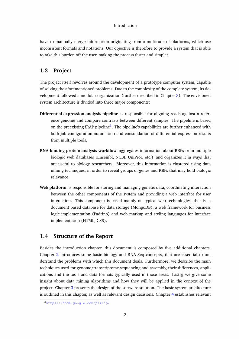
A typical RNA-Seq analysis pipeline is composed by six essential stages [Fas12] (see Figure
2.4):
Read quality control and improvement is a pre-processing stage. It comprises the usage of
quality control tools, whose function is to trim bad quality data, in order to improve the
overall quality of the data set. Other than direct data manipulation, this stage might
produce some statistical data about the reads, that can later be used to better drive the
succeeding stages.
Sample contamination checking is also a pre-processing stage. As read data is obtained
experimentally, it is not uncommon for contamination of the samples to occur. Bacterial
contaminations, such as E. coli, are fairly common and can sometimes skew the analysis
results. In some cases it is possible to detect these contaminations and remove the
affected data, hopefully improving the final results.
1The 1000 Genomes Project, started back in 2008, is an international effort to establish the most comprehensivecatalogue to date of human genetic variations.
10

Problem Domain and Technological Base Concepts
Read alignment is the stage in which reads are positioned against a reference sequence. This
sequence can be either a known and annotated reference genome (typically a combi-
nation of a FASTA file and a GTF file) or an assembled transcriptome, either assembled
de novo or against a reference genome (see Section 2.1.4). This alignment will allow
assessing gene abundance in later stages of the pipeline.
Quantification is the stage where transcript abundance is determined/estimated (gene ex-
pression). This involves counting the number of occurrences of certain transcripts in the
read data. Typically this stage produces transcript count tables, that can later be used
for differential expression analysis.
Differential expression is the stage where transcript abundances between different samples
are compared. As such, the produced count data is used to predict differences between
transcript abundances in two or more samples, effectively demonstrating differences in
gene expression. A common task for differential expression analysis is the comparison
between a control and a mutated sample.
Result reporting is the final stage in most pipelines. In this stage the resulting data is or-
ganized and represented in a manner that is useful to the user. This usually involves
producing plots, tables and reports. Some pipelines may perform additional task before
or after this stage, like gene set enrichment.
Note that this is only a generic architecture of a RNA-Seq analysis pipeline. In practice
new stages can be added and other can be removed, to better suit the experiment at hand and
the available data. In the given example (Figure 2.4) there is an additional stage, gene model
parsing, that is only applied when the read are aligned against an annotated genome.
iRAP
iRAP2 is a RNA-Seq analysis pipeline [FPMB14]. It implements a workflow similar to the one
described above, albeit with some differences (see Figure 2.5). iRAP also allows some stages
of the analysis to be skipped. Differential expression analysis is one such stage. This particular
analysis will only be performed at user request. The gene set enrichment stage (Figure 2.5, in
dashed line) is also optional. This stage uses Piano [VNN13], an R package capable of con-
ducting gene set analysis using various statistical methods, from different gene level statistics
and a wide range of gene-set collections. However, this stage will not be analysed in-depth,
as gene set enrichment was not performed in this thesis.
One of the major strengths of iRAP is the ability to choose the tools that are used in each
stage [FPMB14]. This allows for a vast array of pipeline customization possibilities, making
it easy to adapt to a particular experiment. Below we will present a set of tools, integrated in
iRAP, that were used during this thesis.
2https://code.google.com/p/irap/
11
Problem Domain and Technological Base Concepts
Quality Controland Improvement
Contamination
Read Data (obtained through RNA-Seq)
ID List
Check
Available Reference?
Read Alignment Read Alignment
Predicted or AssembledTranscriptomeGenome
Annotated
QuantificationParse GeneModels
DifferentialExpression
Report Results / Further Analysis
Figure 2.4: Representation of a standard RNA-Seq analysis pipeline [Fas12]. The analysisworkflow has a slight variation depending on whether an annotated genome or an assembledtranscriptome are used as reference for read alignment. Although this is a standard represen-tation of the stages of RNA-Seq analysis, stages can be added or removed as needed to suit aparticular assay.
iRAP requires is a minimum set of user provided information to perform RNA-Seq analysis:
the annotated reference genome and the raw reads, as previously mentioned. Note that the
reads are organized in libraries. A library, in this case a complementary DNA library, is a
collection of cDNA fragments that together constitute a portion of the transcriptome.
12

Problem Domain and Technological Base Concepts
Quality Control(filter reads)
Mapping(align reads against
QuantificationGene SetEnrichment
Read Data (obtained through RNA-Seq)
ID List
Web Reports
reference genome)
DifferentialExpression
Figure 2.5: iRAP RNA-Seq data analysis pipeline. Note that the gene enrichment step (indashed line) is optional and was not used.
2.2.2 RNA Sequencing, Read Alignment and Analysis Tools
We now present some bioinformatic tools, used to support the multiple steps of the RNA
Sequencing, read alignment and data analysis process. It is important to note that none of
these tools were used separately, but rather as parts of an analysis pipeline (also described
below).
Tuxedo Suite
The Tuxedo suite is a free, open-source collection of applications that has been widely adopted
as analysis toolset for fast alignment of short reads. It is composed by four separate tools
(Bowtie, TopHat, Cufflinks and CummRbund) briefly reviewed below. These tools are exten-
sively used for RNA Sequencing analysis. Although the applications are made for command
line execution, there are several workflow managers, like Galaxy3, that easily integrates with
the suite, providing a web interface for its use. Note that not all components of the Tuxedo
Suite were used.
Bowtie. Bowtie is an ultrafast, memory-efficient short read aligner [LTP+09]. Bowtie is
typically used to build a reference index for the genome of the organism being studied, for
posterior use by other tools, like TopHat. It can also output alignments in the standard SAM
format, allowing Bowtie to interoperate with tools like SAM Tools4. However, it should not
be used as a general purpose alignment tool, as it was created and is more effective when
aligning short read sequences against large reference genomes.
3http://galaxyproject.org/4http://samtools.sourceforge.net
13

Problem Domain and Technological Base Concepts
TopHat. TopHat is a fast splice junction mapper for RNA Sequencing reads [TPS09]. It uses
Bowtie as the underlying alignment tool, using its results and a FASTA formated reference
genome to identify splice junctions between exons.
Cufflinks. Cufflinks assembles transcripts, estimates their abundances, and tests for differ-
ential expression and regulation in RNA Sequencing samples [TWP+10]. It uses the SAM or
BAM formatted files as input, typically the ones produced by TopHat, outputting GTF files as
a result.
CummeRbund. Lastly, CummeRbund5 is an R package (see Section 2.3.5) designed to help
the visualization and analysis of Cufflinks’ RNA Sequencing output. As such, it is not directly
involved in the trascriptome alignment process. It takes the various output files from Cufflinks
and uses them to build a SQLite database describing appropriate relationships between genes,
transcripts, and other relevant data points. This database is later used to convert that data to
R objects which allows them to be used by plotting functions, as well as by other commonly
used data visualization tools.
HTSeq
HTSeq is a programming framework used for processing data resulting from next generation
sequencing methods [APH14], developed in Python. While many tools can efficiently align
reads, sometimes data needs to be manipulated before being passed to those tools. These data
can either be badly formated (or “dirty”), or simply in a format different from the one that is
needed. The latter is a particularly common problem when trying to pass the results of one
tool to the one that succeeds it in the pipeline. HTSeq is useful for easily creating scripts that
accomplish this task, acting as a “glue” between tools.
HTSeq provides parsers for many popular formats for representing genetic information
(see Section 2.1.5). In addition, it ships with two standalone scripts, HTSeq-QA and HTSeq-
Count. HTSeq-QA is used to provide an initial assessment of the quality of sequencing runs,
producing plots with that information. HTSeq-Count takes a SAM/BAM file and GTF/GFF file
containing gene models. It then counts, for each gene, how many aligned reads overlap that
gene’s exons.
2.2.3 Differential Expression Analysis Tools
Below we describe the tools that were used for differential expression analysis. These tools
are integrated in the iRAP pipeline, as part of its fourth analysis stage.
5http://compbio.mit.edu/cummeRbund/
14

Problem Domain and Technological Base Concepts
DESeq
DESeq [AH10] is available as an R package (see Section 2.3.5), included in the Bioconductor
super package. DESeq takes count data generated from RNA-Seq analysis assays. As count
data is discrete and skewed, it is not well approximated by a normal distribution. DESeq solves
this problem by applying a test based on the negative binomial distribution, which can reflect
these properties. This method has a much higher power to detect differential expression.
edgeR
edgeR [RMS10] as available in an R package (see Section 2.3.5), included in the Bioconductor
super package. It provides methods for the statistical analysis of count data from comparative
experiments on next generation sequencing platforms, among which is RNA-Seq, the most
common source of data used with edgeR. It has many characteristics in common with the
previously mentioned DESeq, as it also uses negative binomial models (among others) to
distinguish biological from technical variation. Later we describe how both tools can be used
together to produce better results.
2.2.4 File Manipulation and Pre-processing Tools
Sometimes data is badly formated or otherwise in a format that is not compatible with a
specific tool. This is particularly frequent when passing data between two different tools in
a pipeline. As such, we need some intermediate tools that are able to easily manipulate and
transform data, making it useful again. Below we present some tools that can be used to
accomplish this task.
SAM Tools
SAM Tools6 is a library package designed for parsing and manipulating alignment files in the
SAM/BAM format [LHW+09] (see Section 2.1.5). SAM Tools has two separate implementa-
tions, one in C and the other in Java, with slightly different functionality. Beyond manipu-
lation of SAM and BAM files, this package is able to convert between other read alignment
formats, sort and merge alignments and show them in a text-based viewer.
FASTX
FASTX7 (FASTX-Toolkit) is a collection of command line tools for pre-processing short read
files. These short read files can be either in FASTA or FASTQ format. FASTX is used to
manipulate these files before the aligning stage, in order to produce better results. It includes
tools to convert files from FASTQ to FASTA format, assess statistics about the reads, filter and
remove sequences based on their quality, among others. Although the toolkit contains only
6http://samtools.sourceforge.net/7http://hannonlab.cshl.edu/fastx_toolkit/
15

Problem Domain and Technological Base Concepts
command line tools, some of them are already integrated in the Galaxy web based workflow
manager.
FastQC
FastQC8 is a tool for quality control for NGS data, implemented in Java. Its main objective
is to find errors and problematic areas in NGS read data. FastQC accepts FASTQ, SAM and
BAM files, and is able to report results both inside the tool itself and by exporting HTML files.
These reports contain, among other information, summary graphs and tables that allow quick
access to the data. FastQC can either be used as a standalone tool with its graphical interface,
or as part of an analysis pipeline.
2.3 Data Mining
Data mining is the process of “extracting or “mining” knowledge from large amounts of data”
[HKP06, p. 5]. As such, it consists of a set of techniques that can be used to find interesting
patterns in large data sets, that translate in newfound knowledge. Data mining borrows
techniques from multiple fields, such as artificial intelligence, machine learning, statistics, and
database systems [CEF+12]. Its ultimate goal is to combine all those techniques and transform
large and (apparently) meaningless sets of data into understandable and useful information.
Thus, data mining was motivated by the perspective of harnessing the abundance of data, that
characterizes today’s information systems, to produce meaningful knowledge.
Because of their large quantities of input data, data mining tasks are usually totally, or at
least partially, automated. As such, there are several algorithms for these tasks and tools that
implement such algorithms, as presented in Section 2.3.2 and Section 2.3.5, respectively.
We can divide data mining in descriptive data mining and predictive data mining [FPSS96].
Descriptive data mining is focused on finding the underlying structure of a given set of data.
Instead of predicting future values, it concerns the intrinsic structure, relations and inter-
connectedness of the data being analyzed, presenting its interesting characteristics without
having any predefined target. On the other hand, predictive data mining is used to predict
explicit values, based on patterns determined from the data set. With predictive data mining
we try to build models using known data and use those models as a base to predict future
behavior.
As we can see, data mining does not represent a single type problem. In fact there are
several different types of problems that can be addressed by data mining techniques. Each
of these problems may require a different data mining method. A brief review of the most
common type of problems is given below.
8http://www.bioinformatics.babraham.ac.uk/projects/fastqc/
16

Problem Domain and Technological Base Concepts
Classification is a type of problem that tries to generalize the already known structure of a
data set, so that it applies to new data sets. In other words, with classification we try to
learn a function that is capable of mapping our data into predefined classes.
Regression tries to learn a function that models relationships between variables in the data
set. That function can latter be used to find real value predictions of future behavior of
data sets originated from the same population.
Clustering consists in identifying a finite set of categories or clusters of similar values, to de-
scribe the data set. As such, it is used without prior knowledge about the data structure.
Summarization provides a more compact representation of a subset of data, in a way that
the summarized data retains the central points of the original data. This can be accom-
plished in several different ways, like using report generation or multivariate visualiza-
tion techniques.
Dependency modeling finds a model which describes relationships between variables, re-
vealing their dependencies.
Change and deviation detection tries to discover the most significant changes in the data,
when compared with previously measured data. This method is useful for finding inter-
esting data variations or data errors.
Note that due to the nature of the work of this thesis we will focus on clustering analysis
techniques and, as such, the following sections will contain a more in-depth review of these
methods, along with descriptions of the used algorithms and tools.
2.3.1 Clustering Techniques
As explained above, clustering is the process of grouping data into clusters, in such a way
that objects inside a cluster are very similar to each other, while being as different as possible
from objects in other clusters [HKP06]. These similarities (and dissimilarities) are assessed
based on the attributes of each object using a comparison method, often a distance function.
Clustering is used in situations where the classes contained in the data set are unknown, either
because they are difficult to determine or because such an assessment would be too costly or
we known little about the domain and want to do a prospective study.
However, data clustering as a process is highly dependent on the data being analysed. For
example, while some data sets can be easily clustered using “spherical” clusters, other can
only be represented by “concave” clusters. In other words, there is no global technique to
group similar objects, it needs to adapt to the problem at hand. This multitude of different
interpretations of the cluster notion led to the appearance of many different clustering meth-
ods and algorithms. Clustering methods can be classified in different categories: partitioning
methods; hierarchical methods; density-based methods; grid-based methods; and model-based
methods [HKP06].
17
Problem Domain and Technological Base Concepts
Generally, there are two types of clustering methods, divisive methods and agglomerative
methods. In divisive methods all the objects in the data set start in the same cluster. At
each iteration all clusters are divided into two smaller clusters, that better satisfy the fitness
condition of that particular algorithm. This process stops when all clusters are composed by
only one element. Inversely, agglomerative methods start with n clusters with one elements,
joining them iteratively until only one cluster remains.
Partitioning Methods
Partitioning methods are based around the construction of partitions of the whole data set.
Each one of the constructed partitions represents a data cluster. Given a dataset with n ele-
ments, and a number k of clusters, the correct application of these methods must verify two
conditions [HKP06]:
(1) each cluster must contain at least one object (k≤ n);
(2) a single object of the data set must only belong to one cluster.
These methods try to maximize cohesion between objects in the same partition, while
assuring that clusters are as distant as possible between themselves. In other words, the
elements within a partition should be as similar or “close” as possible between them, while
being as different as possible from elements in other groups.
Achieving the optimal partitioning would require the exhaustive enumeration and com-
bination of all possible clusters. This is, of course, impractical and even unfeasible in some
situations. As such, most partitioning methods adopt some sort of heuristic evaluation of their
clusters’ quality. For example, the k-means algorithm uses the mean value of the objects in a
cluster to represent the same cluster; the k-medoids algorithm, which is centroid based, uses
an object that is roughly at the center of the cluster to represent it. Typically these methods
work well with “spherical” clusters, but may falter with clusters having more complex shapes
(“concave” shaped clusters, for example).
Hierarchical Methods
These methods create an hierarchical division among objects in the data set. This hierarchy is
represented as a tree structure. There are two strategies for hierarchical analysis, the divisive
strategy and the agglomerative strategy [HKP06]. The divisive strategy consists of putting all
objects in the same cluster and then divide them in multiple clusters, based on their distance.
Inversely, the agglomerative strategy starts by putting each object in its own clustering, and
then iteratively merges clusters.
One notable weak point of hierarchical methods is that calculated results are irreversible;
that is, once an objects is attributed to a cluster, that result will not be evaluated again.
This may lead to incorrect labeling of some objects. These problems can be minimized by
pre-processing the data set. A possible example of data set pre-processing is performing a
18

Problem Domain and Technological Base Concepts
dimension reduction, decreasing the number of random variables under consideration. Note
that this single pass evaluation gives hierarchical methods good computational performance.
Density-based Methods
Unlike the previous methods that rely on the notion of distance between objects, density-based
methods are based on the notion of cluster density [HKP06]. The basic idea of these methods
is to keep growing a given cluster while the number of objects in its vicinity (or density)
exceeds a certain user defined threshold. Density-based methods are particularly useful to
discover clusters with irregular shapes. An example of an algorithm that implements this kind
of analysis is DBSCAN [EpKSX96].
Grid-based Methods
Grid-based methods transform the data set object space into a finite number of cells, forming
a grid structure [HKP06, Mad12]. All clustering operations are then conducted using the
grid representation of the data set. Algorithms that implement this strategy are usually high-
performance, as execution times are dependent on the number of cells in each dimension of
the grid, rather than on the number of objects in the data set.
Model-based Methods
Model-based methods work by hypothesizing a mathematical model for each cluster and then
finding the objects that best fit those models [Mad12]. These methods typically follow the
assumption that objects are distributed by clusters according to an underlying statistical prob-
ability. This also makes it possible for the number of clusters to be automatically determined,
based on such statistics [HKP06].
2.3.2 Clustering Algorithms
Below we present the clustering algorithms that were used during the progress of this the-
sis. These methods were chosen based on their suitability for the tasks at hand, as will be
described in Chapter 4.
k-Medoids
The k-medoids specification appeared as an evolution of the k-means algorithm. As k-means
uses the mean value of the objects of a cluster to determine its center, it is sensitive to outliers
(objects that deviate considerably from the data set average): an object with a large, dispro-
portional value might skew the results. k-medoids mitigates this problem by using medoids,
picking a specific object of the cluster as its “center” [HKP06]. Medoids are chosen randomly
at the beginning. This means that the algorithm may produce different results depending on
19

Problem Domain and Technological Base Concepts
the starting objects (it does not reach an optimal solution). The remaining objects are then
clustered with the medoid to which they are most similar.
The most common implementation of k-medoids is the Partitioning Around Medoids (PAM)
algorithm (see Algorithm 2.1).
Input: k, the number of clusters; D, a data set containing n objects.Result: A set of k clusters.
choose k objects at random as representatives of each cluster;repeat
assign each remaining object to the cluster with the nearest representative object;randomly select a non-representative object, orandom;compute the total cost, S, of swapping representative object, o j , with orandom;if S< 0 then swap o j with orandom to form the new set of k representative objects;
until no change;
Algorithm 2.1: Partitioning Around Medoids (PAM) algorithm, a k-medoids implementa-tion for partitioning based on medoid or central objects.
Average Linkage Hierarchical Clustering
Average linkage is a method for calculating distance between clusters in the standard hierar-
chical clustering analysis. In order to decide which clusters should be combined or divided,
in agglomerative and divisive clustering respectively, we need a measure of dissimilarity be-
tween those clusters. In the average linkage method this dissimilarity is computed based on
the average distance between all elements in both clusters. The average is calculated over all
pairs of objects composed by one object from the first cluster and one object from the second.
The linkage function is therefore defined as
D(X ,Y ) =1
NX ×NY
NX∑
i=1
NY∑
j=1
d(x i , yi), x i ∈ X , y j ∈ Y (2.1)
where X and Y are two clusters; NX and NY and the number of elements in clusters X and Y ,
respectively; and d(x i , y j) is the distance between objects x ∈ X and y ∈ Y .
Inductive Logic Programming
ILP is a subfield of machine learning that uses first order logic to represent both data and mod-
els [Mug91, LD98]. ILP infers hypotheses (models) from examples and background knowl-
edge. The examples may be of two types: instances of the concept to be “learned” (positive
examples), and non-instances of the concept (negative examples). Background knowledge
is a set of predicates encoding all information that the experts find useful to construct the
models. ILP might be used to tackle several machine learning and data mining problems, like
classification, regression, clustering and association rules discovery.
20

Problem Domain and Technological Base Concepts
The first and most important motivation for ILP systems is that they overcome the repre-
sentation limitations of attribute-value learning systems. Attribute-value systems base their
representations of data in tables. Although effective in many situations, this representation is
not very expressive and might not even be feasible for certain problems [BM95]. The second
motivation for ILP is that by using a logical representation, the hypotheses are understand-
able and interpretable by humans, being therefore useful to explain the phenomenons that
produce the data. This representation also means that background knowledge can be repre-
sented and employed in the induction process, in contrast to attribute-value models, where
this information is difficult to represent. The expressive power of first-order logic enable an
easy representation of data with complex structure, and the encoding of complex models that
may combine numerical computation and relational information.
Despite these advantages, ILP cannot be applied indiscriminately to any clustering or clas-
sification problems. ILP systems are typically very heavy when it comes to computational
resource consumption and run for long periods of time [FCSC03]. To ameliorate this situa-
tion there has been significant progress in parallel execution of ILP systems.
2.3.3 Clustering Evaluation and Assessment
The goal of most clustering methods is to achieve high similarity between objects in the same
cluster, while maintaining the dissimilarity between other clusters [MRS08]. This is called an
internal evaluation criterion, as it is only dependent on the clustered data itself. However, high
internal evaluation scores do not necessarily translate to good results in a real application.
To provide a better judgement of clustering results we may use external criteria [MRS08].
Such criteria act as a surrogate for the judgement of a human field expert. As such, they must
use a set of data outside the clustering data set, that was pre-classified by an expert. This set
of data is considered a golden standard, that is, the best possible outcome for the clustering
analysis, under reasonable conditions.
Note that in the specific case of this thesis no pre-classified data set was available. As
such, we focused our assessments purely on internal evaluation methods. Despite this lack of
automated external evaluation, our results were evaluated by experts in this field, as explained
in Chapter 5.
Silhouette Coefficient
The silhouette coefficient is a direct representation of the intra-cluster similarity and inter-
cluster dissimilarity concept. In other words, the silhouette coefficient improves as the cohe-
sion between elements in the same group and the farthest the distance from that particular
21

Problem Domain and Technological Base Concepts
group to all the other groups [Rou87]. The silhouette coefficient is computed using the for-
mula
s(i) =
1− a(i)b(i) if a(i)< b(i),
0 if a(i) = b(i),b(i)a(i) −1 if a(i)> b(i),
(2.2)
where a(i) is the average dissimilarity between i and all other objects in the same cluster;
and b(i) is the lowest average dissimilarity between i and any other cluster to which i does
not belong. The higher the value of s(i), the more appropriately clustered the data point is.
Inversely, low silhouette values are the result of unfitting clustering. The average s(i) of a
single cluster can be used to measure how tightly all its data points are grouped. The average
s(i) over the entire data set can be used to measure how appropriately the data has been
clustered.
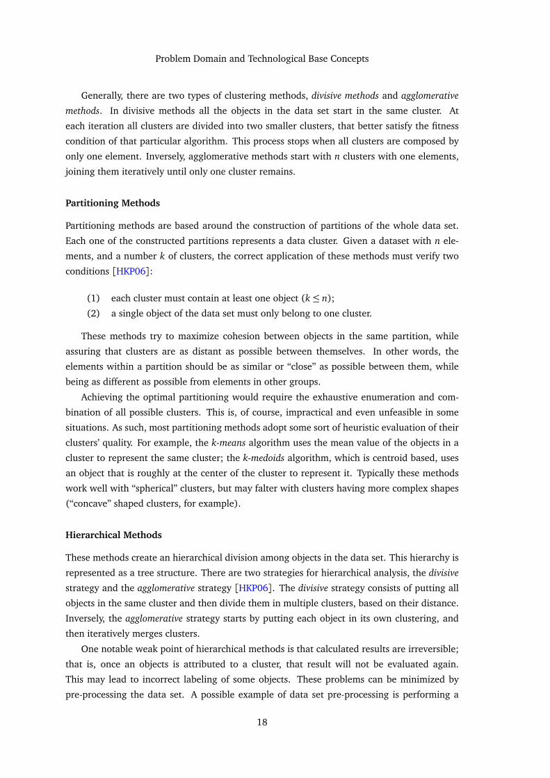
The silhouette coefficient can also be used to provide a visual representation of the clus-
tering results, as dendograms do for hierarchical clustering analysis (Figure 2.6). This plot
combines silhouettes widths for all objects in the data set, the average silhouette width for
each cluster, and the silhouette of the complete data set.
Other than that, the average silhouette of the clustering results may be used to determine
the best number of clusters. This is done by repeatedly executing the analysis with different
k values, between a specified range. The chosen k value is the one that produces the best
average silhouette.
2.3.4 Common Distance Measures
Many clustering algorithms rely on the notion of distance between objects in the data set.
These distances are used as a measure of similarity/dissimilarity between those objects. Typ-
ically, objects that are close to each other are considered similar, as opposed to objects that
are far away from each other and therefore considered different. Below we will present some
common types of distance measures that are used in clustering methods.
Euclidean Distance
Euclidean distance is one the most common distance measures. It represents the geometric
distance between two points, in a n-dimensional space [Mad12]. Euclidean distance can be
defined as shown in Equation 2.3 (for n-dimensions).
d(x , y) =
s
n∑
i=1
�
�x i− yi
�
�
2(2.3)
Squared Euclidean Distance. The squared Euclidean distance is a simple variation of the
standard distance, obtained by squaring it (Equation 2.4). It is used when there is the need
22

Problem Domain and Technological Base Concepts
Silhouette width si
0.0 0.2 0.4 0.6 0.8 1.0
Silhouette plot of pam(x = dataset, k = 4)
Average silhouette width : 0.74
n = 75 4 clusters Cj
j : nj | avei∈Cj si
1 : 20 | 0.73
2 : 23 | 0.75
3 : 17 | 0.67
4 : 15 | 0.80
Figure 2.6: Example of a silhouette plot, using the PAM algorithm. It represents the silhouettesof every objects in the data set, as well as the average silhouette for each cluster (k= 4) andthe average silhouette for the complete data set.
to attribute progressively greater weight to objects that are far apart from each other.
d(x , y) =
s
n∑
i=1
�
�x i− yi
�
�
2
2
=n∑
i=1
�
�x i− yi
�
�
2(2.4)
Manhattan Distance
The Manhattan distance between two objects is the sum of the differences between each of
their components. In other words, it is equivalent to the distance between the two objects, if
a n-dimensional grid-like path was followed [Mad12]. It is defined as shown in Equation 2.5.
23

Problem Domain and Technological Base Concepts
d(x , y) =n∑
i=1
�
�x i− yi
�
� (2.5)
Chebychev Distance
The Chebychev distance is less common than the previously mentioned distances. The Cheby-
chev distance between two objects is defined as the maximum distance between components
of the objects (Equation 2.6). Is is useful in situations where two object must necessarily be
considered different if one of their components is different, as the use of the maximum value
removes the dampening factors of other (closer) components.
d(x , y) =max¦�
�x i− yi
�
�
©
(2.6)
Jaccard Distance
The Jaccard distance is a measure of dissimilarity between two objects. It is related to the
Jaccard coefficient, a similarity measure. In some cases a simple geometric distance, like the
Euclidean distance, might not accurately represent the distance (or dissimilarity) between the
two objects.
For binary attributes, the Jaccard coefficient (similarity) is computed as
sim(x , y) =q
q+ r+ s(2.7)
where q is the number of attributes that are true for both objects; r is the number of attributes
that are true for object x and false for object y; and s is the number of attributes that are
false for object x and true for object y . Note that by definition the similarity coefficient is a
value between 0 and 1, where 0 indicates that the objects are completely different, while 1
indicates that the objects are exactly equal. A distance measure can be obtained directly from
this coefficient, as shown in Equation 2.8.
dist(x , y) = 1− sim(x , y) (2.8)
In this representation a value of 0 is given to two objects that are close, while the value 1 is
attributed to distant objects.
Similarly, the Jaccard coefficient and distance can be computed for sets. This can be
useful to determine distance between to objects whose attributes contain nominal values. The
Jaccard coefficient for sets is calculated as shown in Equation 2.9, while the distance between
sets is calculated in the same way than between binary attributes.
sim(x , y) =
�
�x ∩ y�
�
�
�x ∪ y�
�
(2.9)
24

Problem Domain and Technological Base Concepts
2.3.5 Clustering Tools
Except in rare cases of very specific problems, it typically makes no sense for someone to
implement any data mining algorithm that they might need. In fact, today we have lots of
data mining tools (many of which are free), that already implement many of those algorithms.
These tools are usually customizable, making it easy to adapt them to most problems. Below
we’ll briefly review some of the most popular data mining tools, applicable to the specific
needs of this thesis. Note that some of these tools, namely RapidMiner and Weka, were only
used for testing purposes during the development of the project. As such, they are not part of
the final prototype.
RapidMiner
RapidMiner [rap12] is a complete solution for data mining problems. it is available as a stan-
dalone GUI based application, as seen in Figure 2.7. It is a commercial application, although
its core and earlier versions are distributed under an open source license and it offers a free
version, beyond its multiple paid versions. Being one of the most popular data mining tools
used today, its applications span several domains, including education, training, industrial and
personal applications, among others. Its functionality can also be easily extended through the
use of plugins9, reflecting an increased value for this tool. One of such example in the area of
bioinformatics is the integration plugin between RapidMiner and the Taverna10 open source
workflow management system [JEF11].
Weka
Weka [HNF+09] is an open source tool that implements several machine learning algorithms
and allows its user to easily apply those algorithms to data mining tasks. Created at the
University of Waikato, New Zeland in 199711, it is still in active development to date. Weka
supports several common data mining tasks, like data preprocessing, classification, cluster-
ing, regression and data visualization. Its core libraries are written in Java and allow for an
easy integration of its data mining algorithms in pre existing code and applications. Other
than that, Weka can be used directly through a command line/terminal or through one of its
multiple GUIs (Figure 2.8). Its simple API and well structure architecture allow it to be easily
extended by users, should they need new functionalities.
9Plugin is a software module that adds new functionality to an existing software application. Plugins aretypically dependent on the platform they extend and can’t be used as standalone tools.
10http://www.taverna.org.uk/11The current version was completely rewritten in 1997, despite the first iteration of the tool being developed
as early as 1993.
25

Problem Domain and Technological Base Concepts
Figure 2.7: RapidMiner user interface.
Figure 2.8: Weka interface selection.
R Language
R [Iha98] is a free programming language and software environment for statistical comput-
ing and graphics generation. Originally developed by Ross Ihaka and Robert Gentleman at
the University of Auckland, New Zealand in 1993, it is still under active development. R is
typically used by statisticians and data miners, either for direct data analysis or for developing
new statistical software [FA05].
26

Problem Domain and Technological Base Concepts
R is an implementation of the S programming language12, borrowing some characteristics
from the Scheme programming language. Its core is written in a combination of C, Fortran
and R itself. It is possible to directly manipulate R objects in languages like C, C++, Java
and Prolog. R can be used directly through the command line or through several third party
graphical user interfaces like Deducer13. There are also R wrappers for several scripting lan-
guages.
R provides several different statistical and graphical techniques, including linear and non-
linear modeling, classical statistical tests, time-series analysis, classification, clustering, among
others. It can also be used to produce publication-quality static graphics. Tools like Sweave
[Lei02] allow users to embed R code in LATEX documents, for complete data analysis.
Bioconductor Package. Bioconductor is a free and open source set of tools for genomic
data analysis, in the context of molecular biology [Lei02]. It is primarily based on R. It is
under active development, with two stable releases each year. Counting with more than seven
hundred different packages, it is the most comprehensive set of genomic data analysis tools
available for the R programming language. It contains many of the tools that are part of most
open source biological analysis pipelines. It also provides a set of tools to read and manipulate
several of the most common file formats used in molecular biology oriented applications,
including FASTA, FASTQ, BAM and GFF.
2.4 Chapter Conclusions
In this chapter we gave a brief introduction of the molecular biology concepts that serve as
base of the thesis. We have reviewed the concepts on RNA-Seq and data mining and presented
short analyses of concrete tools and algorithms that were used during this thesis.
12S is an object oriented statistical programming language, appearing in 1976 at Bell Laboratories.13http://www.deducer.org/pmwiki/index.php
27

Problem Domain and Technological Base Concepts
28

Chapter 3
Solution Description
In this chapter we present the designed solution. The main objectives of the solution’s design
are reviewed, along with the most important choices made. Both major components of the
developed solution and their envisioned integration process are described in detail.
3.1 Overview
As discussed, from a purely biological standpoint, this thesis has two objectives: to perform
differential expression analysis of RNA-Seq data and to discover and characterize RBPs related
to groups of genes. While both objectives are important for our particular domain problem,
they present different problems and require different approaches. Furthermore, both parts of
the problem are relevant by themselves.
Splitting the domain problem into two objectives led to the first important design decision.
It was decided that the software solutions to both problems would be implemented indepen-
dently and, at a later stage, integrated with each other, to form the complete system. This
would also allow both tools to be used separately, leading to a wider array of possibilities in
terms of future uses.
Designing software solutions with high performance, scalability and extensibility is also a
major concern. A software solution should be able to quickly and efficiently fulfil a user’s re-
quests, while dealing with a large number of simultaneous users. It should allow new features
to be easily added, in order to better respond to the users’ needs. If these requirements are
not met, the solution is at risk of being abandoned by its users, becoming therefore useless.
The software solutions presented in this thesis were designed with these goals in mind, as is
further discussed in Chapter 4.
29

Solution Description
3.2 Gene Expression Analysis Pipeline
The gene expression analysis pipeline uses iRAP [FPMB14] as its foundation. As discussed
before, iRAP provides begin-to-end gene RNA-Seq data analysis. However, while iRAP is a tool
aimed at a broad group of users, both beginners and advanced users, it is still a command line
tool, with many configuration settings. This technological barrier may drive away some more
inexperienced users. One of the objectives of this part of the work was to make it a simpler
and more straightforward process, accessible to any user with basic computer literacy; another
was to combine results of several different tools, with the aim of improving those results. Note
that some of the features described below were not implemented, due to time constraints. As
such, those features are presented as future work.
3.2.1 Analysis Configuration
iRAP is configured with an experiment configuration file (see Appendix A). This file must
define the name of the species being analysed, the reference and read data files, the tools to
use for the analysis, read libraries, contrast groups, among other variables. Although many
of these configurations are difficult to infer and define automatically, it is possible to create
a more user friendly way to configure the experiments. This is accomplished through a web
form. This web form has two different views: the normal view allows users to configure only
the essential settings of the experiment, those that cannot be inferred; the advanced view
allows more experienced users to tweak every configuration.
3.2.2 Experimental Data Management
Gene expression analysis with iRAP requires two sets of files, reference files and read data files.
Reference files are both the reference genome (in FASTA format) and its annotations (in
GTF or GFF formats). These files are automatically obtained from Ensembl’s FTP endpoint.
The current release contains information of a total of sixty six species. The tool automatically
checks if a new release is available, and in that case downloads and substitutes the files. In
the experiment configuration users need only to indicate which species they are analysing,
and the correct files will be automatically passed to iRAP.
Read data files contain the reads obtained through sequencing, in FASTQ formats. The
user needs to upload these files. One file must be provided for each library the user wants to
analyse, and should be compressed. As some of these files can be quite large, users also have
the possibility to provide a link to those files. If a link is provided, the files will be downloaded
before the analysis starts.
3.2.3 Analysis Workflow
Once both the configuration file and the required data files are ready, the analysis process can
begin. The analysis process starts by passing those files to iRAP (Figure 3.1). In this initial
30

Solution Description
stage of the workflow the analysis will stop immediately after the quantification step (see
Section 2.2.1).
ID List
Differential Expression Results
Read Data Reference Data
Base Analysis
Differential Expression(edgeR)
Differential Expression(DESeq)
Combine Results
Figure 3.1: Gene expression analysis pipeline workflow.
The next step is to sequentially execute differential expression analysis with the chosen
tools, in this case DESeq [AH10] and edgeR [RMS10]. The resulting files are kept until
all tools are executed. Note that there is no need for the analysis process to start from the
beginning every time a new tool is used, as iRAP can (in most cases) reuse the results produced
up until the point where a new tool is introduced.
After all tools are executed their results must be combined into a final list of gene identi-
fiers. This is done in an attempt to give researchers an higher level of confidence in differential
expression results. Note that this process is not part of the iRAP analysis pipeline, and there-
fore a new tool must be developed. Algorithm 3.1 shows the basic process of combining the
obtained differential expression results. First, entries in every file must be filtered by their
p-value1, that must be inferior to a maximum threshold (0.05 by default). Then all entries
1A p-value is used to assert the statistical significance of results. It represents the probability of obtaining thesame results as before in a new sample, given that the null hypothesis is true [Goo].
31

Solution Description
in all files are compared with each other. This produces an intersection of all files, in other
words, a list of entries that are present in all files.
genes = empty map;files = load all result files;max_pvalue = 0.05;foreach file in files do
foreach entry in file doif entry.pvalue ≤ max_pvalue then
increase gene count in genes[entry.gene];end
endendforeach gene, count in genes do
if count < number of files thenremove gene from genes
endendwrite genes to a file;
Algorithm 3.1: Combination of differential expression results.
3.3 RNA Binding Protein Analysis Web Platform
The main objective of this system is to transform a complex, manually performed analysis,
into an automated workflow. The platform should require as little information as possible
from the user, inferring analysis parameters whenever possible. It should also be able to
automatically group genes (and proteins), to reveal implied relationships between them that
might be useful to experts. This platform was named Protein Binding Site Finder (PBS Finder)
and shall henceforth be referred to by that name.
3.3.1 Experimental Data
The only data PBS Finder collects from the user is a list of gene (or transcript) identifiers that
should be analysed. These identifiers can be in one of five different formats: Ensembl Gene,
Ensembl Transcript, Entrez, RefSeq or GenBank (see Table 3.1). Users can submit jobs with any
combination of the previous types and use identifiers from multiple species.
Table 3.1: Two sets of examples of identifiers accepted by PBS Finder.
Ensembl Gene ENSG00000224274 ENSRNOG00000013536Ensembl Transcript ENST00000003156 ENSRNOT00000117589Entrez 11245 66850RefSeq NM_001107622.1 NM_031098.1GenBank U49845 C35522
32

Solution Description
While PBS Finder can accept all these kinds of identifiers, internally the analysis can only
be started with Ensembl Gene or Entrez identifiers, that map to Ensembl’s and NCBI’s pages, re-
spectively. As such, the identifiers must be first separated into different groups and converted.
This conversion is reviewed with more detail in Section 3.3.3.
3.3.2 User Information Management
In order to use PBS Finder a new user must create an account, providing their name and
email, and choosing their authentication password. The account system was implemented so
that jobs could be associated with their creator in a cross browser/system manner, in contrast
with a typical cookie-based2 data persistence. This allows each user to list their own jobs.
Despite jobs being only directly accessible by their owner (creator), no effort was made to
deny users access to each other’s jobs through the job’s URL. We believe that sharing results is
an essential part of the investigation process.
To create a new job the user provides a job description and an identifier list. The identifier
list is a newline-separated list (a single entry per line) of unique identifiers for genetic infor-
mation databases. In the current version acceptable types of identifiers include Ensembl (both
Gene and Transcript), Entrez, RefSeq and GenBank. Users can submit jobs with any combina-
tion of the previous types and use identifiers from multiple species. Upon job creation, users
can choose to be notified by email when the job finishes.
3.3.3 Analysis Workflow
PBS Finder is based on a three stage analysis model (Figure 3.2): base analysis, data set
enrichment and clustering analysis.
Job Data
ID List
Base Analysis ClusteringEnrichment
Transcript Data Protein Data Cluster Info
Figure 3.2: Simplified PBS Finder workflow.
2Modern websites sometimes need to save information about the user, for example credentials. This data canbe saved in the client machine, through the use of a web browser cookie.
33

Solution Description
Base analysis comprises data set filtering, retrieval of basic gene and transcript information
and finding RBPs. The first released version of the platform implemented only this stage of
the analysis. It contains all the information that is necessary to answer one of the base thesis
problems. However, further stages build on top of this information, bringing a more valuable
set of results to biologists.
In the enrichment stage additional information about every protein is retrieved. This
information is obtained from UniProt3, a web platform for curated protein information. This
stage was implemented in the second release of the platform.
The clustering stage takes all the information collected in the previous stages and uses it to
perform clustering analysis. There are two types of clustering analysis performed: clustering
using RBP presence and clustering using RBP attributes. The objective of this analysis is to
uncover implicit relationships in the collected data, that may be of use to biologists.
These stages are described in more detail in Chapter 4.
3.4 Tool Integration
In the designed solution both tools should be integrated, so that a user could perform the
complete analysis creating a unique analysis job. This would be accomplished by using the
interface of the RNA-Seq analysis pipeline as the master (or main) interface for job creation.
When the analysis completes, the pipeline presents the preliminary results to the user and
automatically launches a PBS Finder analysis for the resulting gene identifier list. At this
point the RNA-Seq pipeline’s interface should include a direct link to the created job in PBS
Finder. That link can then be used by the user to view the results of the RBP localization
analysis. Note that, while both tools are now integrated, the results of both analyses are
independent. As such, they can be consulted/reviewed independently from each other, as if
both had run separately.
3.5 Chapter Conclusions
In this chapter we reviewed the most important details about the design of the proposed
software solution (implementation details are described in Chapter 4). We presented the
modular, two subsystem model, that allows both tools to be used as standalone products,
increasing the number of their possible uses. Lastly, we talked about the general details of the
workflows of both tools, as well as the integration of those workflows.
3http://www.uniprot.org
34

Chapter 4
Implementation
In this chapter we present and discuss some specific details of the implementation of the
designed solution. We will also review some of the used technologies, and provide the rational
behind their choice, whenever relevant.
4.1 Gene Expression Analysis Pipeline
Due to time constraints the gene expression analysis pipeline could not be fully finished.
Integration with PBS Finder’s analysis pipeline was not accomplished. Similarly, it was also not
possible to provide the RNA-Seq analysis pipeline’s functionality through the web interface.
However, both the iRAP pipeline and the results combining program were completed and
functional.
4.1.1 Combining Differential Expression Results
The results combining tool was implemented in the form of a Ruby script. As a command
line script this tool can be easily integrated with the existing iRAP workflow, as iRAP is also
completely executed in the command line.
The results of differential expression produced by iRAP are exported as tab-separated val-
ues (TSV) files. Each differential expression analysis tool produces a TSV file for each contrast
that is analysed. These files contain gene identifiers and a variety of statistical values for each
identifier, including the p-value.
The tool takes all files from a single contrast, filters entries by p-value and counts the num-
ber of times each gene identifier is found. Note that each file has at most one occurrence of
a gene identifier. Every identifier that appears in all files is exported to the text file that con-
tains the combined results. This file can then be used as input for the RBP analysis platform,
obtaining further information about those genes.
An example of the use of this module is provided in Section 5.1.2 of Chapter 5
35

Implementation
4.2 RNA Binding Protein Analysis Web Platform
PBS Finder is implemented in two parts, following a client-server architecture: the web inter-
face and the analysis server. In this case the web interface is the client and the analysis server
is the server. This means that, whenever a user submits an analysis job, the web interface
sends an analysis request to the server, including the data set given by the user. The server
then processes the request and reports the results back to the web interface, that presents
them to the user.
4.2.1 Web Interface
PBS Finder’s web application interface is written in Ruby, using the Padrino1 framework.
Padrino is a web framework built on top of the Sinatra2 web library. Padrino allows the
creation of web applications that use Ruby to define their back-office logic.
4.2.2 Data Persistance
User and job data is persisted in a database; in this case the MongoDB3 database system
was chosen. MongoDB is a document based, NoSQL database. While widely adopted rela-
tional database management systems rely on large data banks and relational calculus, NoSQL
databases store information in the form of documents [SSK11], instead of relational table
records. NoSQL databases sacrifice the possibility to use some complex mechanisms of classi-
cal relational databases (for example structured queries and enforced information integrity),
in order to achieve higher performance and scalability. NoSQL databases are most effective
when the saved records are large but are seen as loosely structured collections of information.
4.2.3 Analysis Server
The analysis server is responsible for managing analysis requests sent by the web interface.
The server is implemented on top of Distributed Ruby (dRuby), a distributed object system
for Ruby. dRuby allows methods and behaviours to be invoked on an object that exists in
a different process or even in a different computer, using a network connection. From the
client’s point of view it seems like the object is local, as it can be used as any other object. The
server uses a master distributed object to receive analysis requests from the web interface.
The server launches each job concurrently. This behaviour allows the server to run multi-
ple analyses at the same time. Note that the server is not bound to a single type of analysis,
it can perform any type of analysis, as long as a valid implementation is available. The only
two constraints to create a new type of analysis are that the analysis workflow must be encap-
sulated inside an instantiable class. That class must implement a defined interface, in other
1http://www.padrinorb.com2http://www.sinatrarb.com3http://www.mongodb.org
36

Implementation
words, it must implement a simple set of methods that allows the server to control it. As
such, new analysis methods can be easily added in the future as their core functionality can
be opaque to the server as long as they implement the server’s interface.
Algorithm 4.1 represents the behaviour of the server when a new request arrives. The first
step is to determine if the requested analysis method is available. If it is, the corresponding
class is instantiated, and the analysis data set (and other relevant information) is passed to it.
Note that at the same time the server creates a file with a copy of all the parameters of that
particular request. If for some reason the server stops working, analyses that were running at
that time will be automatically restarted once the server is available again. After the object
that will be responsible for the analysis is created, the server creates and starts a new thread
for it. The server also saves an indication that that particular analysis is being executed.
receive request;if request.analysis_method is available then
instantiate request.analysis_method with request.parameters;save request.parameters to disk;run the analysis in a new thread;if success then
report results;else
report error;enddelete request.parameters from disk;
elsereport error;
end
Algorithm 4.1: Processing a new analysis request from the web interface.
Once the analysis is complete the server is notified through its distributed instance, and
the results are communicated to the web interface. This also prompts the server to eliminate
both the indication of the running analysis from its internal list and the file with the analysis’
parameters from the file system.
4.2.4 Analysis Workflow
A detailed overview of the RBP analysis workflow can be seen in Figure 4.1. This workflow is
composed by three main stages: base analysis, data set enrichment and clustering analysis, all
of which will be described in detail below.
4.2.5 Base Analysis
The first step in the pipeline is to prepare the gene identifiers for the following analysis steps.
These identifiers can be written in five different notations, as described in Section 3.2.3. As
such, identifiers are separated according to their automatically detected notation in those five
37

Implementation
Ensembl Gene ID
Ensembl Transcript ID
Ensembl Gene ID List
Entrez ID
RefSeq ID
GenBank ID
Preliminary ID Matching
Entrez ID List
Convert to Ensembl Gene IDConvert to
Entrez ID
Convert toConvert to
Ensembl Gene ID
Gene Enrichment
Group Genesby Species
Find RBPsQuery RBPDB
UniProtEnrichment
KEGGEnrichment
CollectKEGG IDs
RBPClustering
RBP ClusterCharacterization
ClusterSelection
Gene ClusterCharacterization
GeneClustering
ClusterSelection
ID List
ID List
Base Data Set
Intermediate Data Set (with RBPs)
Enriched Data Set
Results
Figure 4.1: PBS Finder workflow. Note that error paths were not represented for simplicity.However, every component implements health checks, that may stop the entire analysis if theminimum requirements for success are not met.
38

Implementation
groups. However, some of those identifiers may be invalid, despite appearing to fit in one of
the possible notations. It is assumed that if an identifier is valid, it can at least be converted
to either Ensembl Gene or Entrez notation. These notations were chosen because they are
the native notations for genes in the used platforms (Ensembl and NCBI). This conversion is
done using bioDBnet’s [MCYS09] identifier conversion service. The service was chosen for
its simplicity and its large conversion database, that draws from multiple conversion services
like NCBI or Ensembl. Entrez conversion is only attempted if Ensembl Gene conversion is not
available. While none of those platforms are preferred, converting as many identifiers as
possible to one convention helps to maintain data set coherence.
Since only two lists remain, one with Ensembl Gene identifiers and the other with Entrez
identifiers, information about those genes’ transcripts must be collected. This information in-
cludes the transcript’s name, its identifier, and its relevant genetic sequences. This information
is collected using their corresponding platform (Ensembl or NCBI).
The transcript sequences are then used to retrieve the related RBPs using RBPDB, an online
RNA binding protein database [CKZ+11]. For each sequence RBPDB finds every possible
RBP, along with its name, location and binding sequence. A complete list of all information
retrieved for both genes and transcripts can be found in Table 4.1. For a specific transcript,
if the retrieved 3’ UTR sequence is at least three hundred base pairs long it will be used with
RBPDB. If the 3’ UTR is too short, the 3’ UTR downstream sequence (genomic sequence) will
be used, with a fixed length of one thousand base pairs. If none of the above situations is
possible, the 3’ UTR will be used as is (if it is at least one base pair long). Note that while
the 5’ UTR sequence is also collected (when available), the consulted experts were interested
in analysing only the 3’ region. This information is sufficient to answer one of this thesis’
problems. However, it will be enriched and further analysed, bringing greater benefits to
researchers.
Table 4.1: Information retrieved for genes and transcripts in the base analysis stage. Informa-tion marked with “*” represent optional information; it might be relevant to the researcherand is therefore shown if available, but it is not crucial to the analysis. On the other hand,the unmarked fields represent required information, without which analysis on that particulargene/transcript cannot continue.
GeneTranscript identifiersGene name*Species*
TranscriptProtein identifiersTranscript name*Genetic sequences (3’ UTR, 3’ UTR downstream, 5’ UTR)Names, locations and bind sequences of RBPs
39

Implementation
4.2.6 Data Set Enrichment
Given the RBP names obtained in the base analysis stage, a query is made to UniProt in order
to obtain their respective accession identifiers. These are used internally by UniProt to refer to
specific proteins. With the accession identifiers, the pages for each RBPs can be retrieved and
analyzed individually. These pages contain information about their respective RBPs, including
keywords, related tissues and information about the RBPs’ ontologies (cellular components,
molecular functions and biological processes).
The information collected from UniProt may also contains links to the KEGG web plat-
form. Among other useful information, KEGG contains information about protein pathways.
A pathway is a sequence of actions, related to specific molecules, that produce certain changes
within a cell, when performed. This information is crucial to understand the function of RBPs.
As such, it is collected for further analysis (see Table 4.2 for a complete list of all information
retrieved).
The first step for this phase is to use the protein names to retrieve a list of matching
UniProt Accession identifiers. By default PBS Finder will try to find a reviewed accession whose
species matches the species in question. If this is not possible it will fallback to an unreviewed
accession, from the same species. In case this is also not possible, it will try to find a reviewed
human analogue accession or, as a last case, an unreviewed one. After finding the identifiers,
the batch retrieval service is used to enrich the protein information. This information includes
ontologies, related tissues, and references to external databases. From these references, KEGG
identifiers in particular are used to retrieve information about pathways in which the RBPs
are expressed. For each pathway, both its name and link to the KEGG pathway viewer are
provided.
Table 4.2: Information retrieved for proteins in the data set enrichment stage. Informationmarked with “*” represent optional information; it might be relevant to the researcher andis therefore shown if available, but it is not crucial to the analysis. On the other hand, theunmarked fields represent required information, without which analysis on that particularprotein cannot continue.
Protein
Protein nameUniProt identifierAccession speciesRelated tissues*Keywords*Pathways*Ontologies*URLs to external platforms*
40
Implementation
4.2.7 Clustering Analysis
The last stage of the workflow is clustering analysis. Two different types of clustering ap-
proaches were conceived: clustering by RBP presence and clustering by RBP information. Note
that this analysis will not be performed if the quantity of available data is below certain
thresholds (typically the tool will not analyse data sets that have less than ten genes and/or
ten RBPs).
Clustering by RBP Presence
In the first case, the clustering analysis is only conducted at the gene level. Two genes are
similar if they are associated with the same RBPs. Inversely, two genes that do not have any
(or few) RBPs in common are considered “distant”. The tool makes an additional step in order
to determine which RBPs are common in one particular group, while being absent in all the
other groups. This information allows researchers to easily determine which RBPs can be used
to interact with a particular group of genes, while not affecting the others.
Clustering by RBP Information
In the second case the clustering process has two phases. In the first phase RBPs are grouped
based on their similarity. Similarity is computed using a set of attributes that include (de-
pending on availability): pathways; tissues where the RBP is expressed; keywords describing
their main functions; and other relevant information such as ontologies (biological processes,
molecular function and cellular components). The tool compiles a list of defining features for
each group (to later present to the user). However, in this case the RBP groups will be used to
group similar genes. Unlike the previous method, similarity between genes is not only mea-
sured in how many RBPs they have in common. In this case any two genes may be considered
similar if both are related to RBPs that were grouped together in the previous step, even if
they do not share exactly the same RBPs between them.
Setup Variation
To produce the final results multiple clustering experiments are attempted. Due to the small
amount of time that the chosen clustering algorithms need to run it is possible to execute
a large number of attempts and then choose only the best results. Each attempt is a varia-
tion of the analysis parameters, being that each possible value for a parameter is combined
with every value for the remaining parameters, giving rise to a large number of experiments.
When clustering by RBP presence the variable parameters are: clustering algorithm (either
hierarchical clustering or partitioning around medoids); and the number of clusters (between
two and ten). While clustering by RBP information the same variable attributes apply. How-
ever, the decision about what RBP information is used for their comparison is also variable,
from a minimum of two information fields. For example, in a particular clustering attempt
41

Implementation
only information about the RBPs’ pathways and related tissues may be used, while another
attempt may use all available information. Furthermore, for this particular type of analysis
the representation of the data set can also vary. The data set can be represented either as a
binary matrix (as is the case in clustering by RBP presence) or by a Jaccard distance matrix,
calculated from the sets of possible values for each of the protein’s attributes.
Result Selection
With the large number of results obtained from all the clustering attempts, it is not reasonable
to expect a user to manually choose the ones that are most interesting. As such, internal evalu-
ation techniques for clustering are coupled with rules that define minimum acceptance criteria
for results, narrowing the result space to only one for each type of clustering. Algorithm 4.2
represents the method used for result selection.
sort clustering results by average silhouette (descending);filter clustering results with clusters with less than 8% of data set objects;abundance_frequency = 0.90;while abundance_frequency ≥ 0.50 do
foreach clustering result doclassify as abundant any attribute with frequency ≥ abundance_frequency;remove abundant attributes that appear in multiple clusters;if at least one unique abundant attribute exists for each cluster then
select cluster;break loop;
elseabundance_frequency = abundance_frequency − 0.05;
endend
endif a cluster was selected then
return selected cluster;else
return cluster with highest average silhouette;end
Algorithm 4.2: Selection of best clustering results.
ILP Clustering
Clustering using ILP techniques was also attempted. The main objective of this approach was
to uncover more information about the implicit relationships present in the data sets. While
conventional clustering methods present only the data set objects grouped in clusters, with
ILP it is possible to understand exactly what rules were used to form those clusters.
The devised approach had two steps. First, the results for each new job would be repre-
sented in the form of Prolog clauses. Second, those clauses would be used as data set for the
42

Implementation
ERDA [FCC12] clustering system, running on top of YAP Prolog [CDR11]. However, due to
problems with the available tools, this approach could not be included in the current version
of PBS Finder.
4.2.8 Web Interface
Job View
Job view, also known as main view, is the default projection of a job’s results (Figure 4.2).
It gives the user a matrix that matches every gene (and transcript) in the data set with their
corresponding binding proteins, as well as an histogram of the genes (a bar chart of the
number of genes with which each RBP binds). This matrix also contains two columns that
provide information about how the genes were grouped, based on the two distinct clustering
techniques. In addition to this information, clicking any group of genes will give the user a
list of all the characteristics that differentiate that particular group from all the others.
This view also contains a mechanism that allows users to provide feedback and report
problems. Clicking the “Report a problem” button the user is presented with a form that
allows them to provide a brief description of the problem. If the user chooses to send that
report, the web platform will send an email to its administrator, containing the submitting
user’s information, the problem description and a direct link to the offending page.
Transcript View
The transcript view (Figure 4.3) offers more detailed information about the transcript’s bind-
ing proteins, giving for each protein the base pairs that compose the binding site (and its
start and stop positions) and a percentage score of the match’s quality. A maximum of three
different genetic sequences (5’ UTR, 3’ UTR and 3’ UTR downstream4) are also displayed,
depending on their availability. Whenever possible, related links to other platforms are pre-
sented (Ensembl, NCBI and UniProt). Like the job view, it also contains clustering information,
but in this case only one column, that shows how the RBPs related to that specific transcript
were grouped. Also similarly to the job view, users can click any group to obtain relevant
information about the defining characteristics of that particular group.
Protein View
The protein view (Figure 4.4) displays relevant classification information for every RBP (when
available). This information includes the protein’s name, links to other platforms (UniProt,
KEGG, Gene3D, etc.), tissues in which the protein might be expressed, the protein’s ontologies
and the pathways in which the protein participates. Each pathway is coupled with a link to
the corresponding KEGG pathway browser page.
45’ UTR and 3’ UTR are non-coding regions located before the initiation codon and after the terminationcodon, respectively. While these regions are not translated to useful genetic products, their presence is importantto regulate cellular processes.
43

Implementation
Figure 4.2: Job view example, also known as main view. It is comprised by three maincomponents: general information (which includes data download); RBP frequency histogram;and RNA binding protein matching table.
Exporting the Results
Besides browsing, users can download their results as text files. Three different types of data
projections of the results are provided: RBP data, protein data and the complete data set. RBP
data can be downloaded in either comma-separated values (CSV) or tab-separated values
(TSV) format. This file gives the user a match matrix of binding proteins, similar to the one in
the job results view, as well as species, gene and transcript information. Protein data can also
be downloaded in both CSV and TSV formats. It gives a more complete view of the results,
including species, gene, transcript and protein identifiers and additional protein information
44

Implementation
Figure 4.3: Transcript view example. It contains four main areas: general information aboutthe transcript; RNA sequences (5’UTR, 3’UTR and 3’UTR downstream are shown dependingon availability); RBP locations histogram; and RBP location table (including clustering resultsand match sequences).
(keywords, related tissues, ontologies, etc.). Finally, the data set may be downloaded as a
complete Prolog predicate representation of the job results. This is the same representation
of the results that was created with the usage of ILP clustering techniques in mind. While it
was not possible to use those techniques, the produced data set representation might still be
of use to researchers.
While in most cases these data representation conversions are apparently instantaneous,
for large data sets they may take an additional amount of time. This would cause the web
application to seemingly block if the user tried to download one of those files. To solve this
problem all files are generated during the analysis process, then stored in the web application’s
45

Implementation
Figure 4.4: Protein view example, containing four relevant areas: general information aboutthe protein; links to other web platforms with relevant information about the protein (notethat some of those platforms might not contain information about a particular protein, andtherefore no links can be shown); additional info, including keywords, related tissues andpathways in which the protein is expressed; and lastly, information about the protein’s on-tologies, including cellular components, molecular functions and biological processes.
MongoDB instance through GridFS5. This allows those files to be downloaded instantly, as
they need only to be generated once.
4.3 Chapter Conclusions
In this chapter we presented a concrete approach to the development of the proposed so-
lutions. We reviewed their most important features and implementation choices. Further
examples of their usage is available through a case study in Chapter 5.
5GridFS is a functionality integrated in MongoDB that allows a simple file system to be simulated inside adatabase. Files are divided into small chunks and those chunks are stored as regular MongoDB documents.
46

Chapter 5
Case Studies
In this chapter we present two case studies that were used as a proof of concept for the
developed system. We characterize the experimental environment, the used data sets and the
obtained results for both cases. We then compare the developed solutions with the previously
available methods.
5.1 Gene Expression Analysis Pipeline
This case study illustrates the developed gene expression pipeline, composed by iRAP and the
differential expression results combination tool. Gene expression analysis is a complex task
and, because of that, no definitive tool exists that can produce good results for every possible
case. Some tools are better when analysing certain types of data/organisms, while other tools
might have other strengths and weaknesses. It is difficult for an inexperienced user, as it is to
an automated tool, to determine the best tool to use in each case. The objective of this case
study is to ascertain if the developed pipeline enhancement can help overcome this difficult,
by combining the best results from multiple tools.
5.1.1 Case Study Setup
The data used in this case study was obtained from Ensembl Genomes (annotated reference
genome) and ENA Sequence Read Archive (sequencing reads). The experiment itself is based
on RNA-Seq experiment E-GEOD-48829, available at ArrayExpress1.
1ArrayExpress in an online database where researchers can submit and search functional genomics experi-ments. This particular experience can be found at http://www.ebi.ac.uk/arrayexpress/experiments/E-GEOD-48829/.
47

Case Studies
Analysis Data Set
The used data set was the same as in ArrayExpress experiment E-GEOD-48829. This exper-
iment studies the Escherichia coli bacteria, commonly known as E. coli. E. coli is a model
organism: a “simple”, non-human organism that is extensively studied, with the expecta-
tion that the discoveries made for that particular organism are useful to understand different
organisms [FJ05]. Other examples of model organisms are Rattus norvegicus (norway rat),
Drosophila melanogaster (fruit fly) and Mus musculus (common mouse).
Being extensively studied was just one of the reasons that led to this choice of data set. As
a single cellular organism, E. coli is a simple organism, whose genome is fairly short (when
compared with vertebrates, for example). This allows for much faster analysis times of a few
hours, as opposed to the longer run times of larger genomes.
The experiment was composed by a total of six libraries, divided into two groups. These
groups were used to define a contrast2 in the differential expression analysis.
Experimental Environment
For this data set all tests were performed in the same machine. The machine’s specifications
can be consulted in Table 5.1. Performance was not a big concern in this case study, as it is
expected that iRAP may takes between hours and days to complete an experiment. In these
experiments the biggest constraint is the machine’s memory: older machines might not have
enough memory to execute a complex iRAP analysis.
Table 5.1: Specifications of the test environment used for the case study experiments.
MachineOperative system Debian GNU/Linux Jessie/SidCPU Intel Core 2 Quad Q9400 (4 cores)CPU speed 2.66 GHzMemory 16 GiB DDR2 (800 MHz)
Methodology
Firstly, all information related to the experiment was downloaded to the test machine (an-
notated reference genome and reads). A configuration file for the experiment was written,
defining settings, libraries, groups, contrasts and any other information relevant to the exper-
iment.
The experiment was then executed until the quantification step; no differential expres-
sion analysis was performed at this point. This preliminary experiment used TopHat as a
mapping/alignment tool and HTSeq as a quantification tool (see Section 2.2.2).
2In the context of differential expression a contrast is composed by two groups of libraries; these groups arecompared between them, in order to uncover differences in their expression levels.
48

Case Studies
Differential expression analysis was then performed using the previously produced quan-
tification data. This analysis was conducted with both edgeR and DESeq (see Section 2.2.3).
The total number of distinct lines in each result file was counted (for both tools). The next
step was to remove any entries with high p-values from those files, leaving only lines with a
p-value less or equal to 0.05. New line counts were produced for each of the filtered files.
Finally, both files were combined in a single using the produced tool, and a last line count was
made.
5.1.2 Comparison with Previous Results
The developed tool’s results were compared with both the normal “raw” results directly pro-
duced by the differential expression tools and with those same results, filtered by p-value.
Table 5.2 shows these results, in terms of distinct lines per results file. Note that every line
corresponds to a unique differentially expressed gene.
Table 5.2: Number of distinct lines resulting from differential expression analysis. Theseresults are relative to the raw results produced by the differential expression tools, thosesame results filtered by p-value and combined with the produced tool.
Raw results Filtered results Combined resultsedgeR 4494 386
191DESeq 4494 204
This experiment demonstrates that the developed tool can in fact filter the results of dif-
ferential expression into a smaller data set. This filtered data set will hopefully reveal itself
more useful to researchers, eliminating unnecessary information and giving higher levels of
confidence in the results. However, we have no way of comparing these results with the pre-
vious ones from a biological standpoint. Such assessment must be performed by experts in
this field, which was not possible at this time.
5.2 RNA Binding Protein Analysis Web Platform
This case study is aimed at the RBP analysis tool (PBS Finder). RhoGTPases comprise a family
of molecular switches that control signal transduction pathways that link cell surface receptors
to a variety of intracellular responses. In this particular case the genes are related to the
well known model organism Rattus norvegicus, commonly known as norway rat. This data
set was produced by IBMC experts. The same experts then validated the obtained results
experimentally.
This experiment has three distinct goals. The first goal is to assess the general usefulness of
PBS Finder. It is important to determine if the developed tool can at least reproduce the results
obtained with previous methods. It is also relevant to assess if PBS Finder is able to provide
even more relevant information to researchers, facilitating their work. The second goal is
49

Case Studies
to compare PBS Finder with the existing techniques of manual analysis. One of the major
constraints of manual analysis is the time it takes to complete; PBS Finder should be able to
reduce the duration of the analysis. Lastly, the third goal is to assess the impact of differences
in hardware performance in the overall performance of the platform. PBS Finder should
be sufficiently optimized to be able to run in personal computers with decreased hardware
performance, instead of only in servers or computer clusters.
5.2.1 Case Study Setup
The available case study data set was produced by IBMC experts. The same experts then
validated the obtained results experimentally.
Analysis Data Set
The analysis data set is comprised by twenty three gene identifiers, from the RhoGTPase family.
The actual genes used for our tests can be found in Table 5.3. Note that the tool only needs
to receive gene identifiers; gene names are not currently accepted as input data.
Table 5.3: RhoGTPase family genes used as data set in the case study.
Gene name Gene ID Transcript IDRhoj ENSRNOG00000021919 ENSRNOT00000031979Rhog ENSRNOG00000020393 ENSRNOT00000027641Rac3 ENSRNOG00000048172 ENSRNOT00000073886Rac2 ENSRNOG00000007350 ENSRNOT00000009994Rhod ENSRNOG00000019220 ENSRNOT00000026092Rhof ENSRNOG00000042607 ENSRNOT00000064390Rhoh ENSRNOG00000002540 ENSRNOT00000003425Rnd ENSRNOG00000020698 ENSRNOT00000028089Rhoc ENSRNOG00000012630 ENSRNOT00000017254Cdc42 ENSRNOG00000013536 ENSRNOT00000029025Cdc42 ENSRNOG00000013536 ENSRNOT00000018118Rhoq ENSRNOG00000015415 ENSRNOT00000020822Rac1 ENSRNOG00000001068 ENSRNOT00000001417Rhou ENSMUSG00000039960 ENSMUST00000136615Rhou ENSMUSG00000039960 ENSMUST00000045487Rhoa ENSRNOG00000050519 ENSRNOT00000071664Rnd1 ENSRNOG00000013621 ENSRNOT00000018276Rnd3 ENSRNOG00000004624 ENSRNOT00000006111Rhob ENSRNOG00000021403 ENSRNOT00000008008Rhobtb1 ENSRNOG00000000633 ENSRNOT00000000784Rhobtb2 ENSRNOG00000017373 ENSRNOT00000023876Rhobtb3 ENSRNOG00000012414 ENSRNOT00000016838Rhov ENSRNOG00000013380 ENSRNOT00000018277
50

Case Studies
Experimental Environment
The testing environment was reproduced in two different machines. These machines differ in
their hardware and operative system, but every other variable in the environment (internet
connection speeds, machine usage, etc.) holds for both machines. Performance results for the
case study experiment for both machines are given in Section 5.2.4. Henceforth the machines
will be referenced as Machine1 and Machine2, as shown in Table 5.4.
Table 5.4: Specifications of the test environments used for the case study experiments.
Machine1 Machine2Operative system OS X 10.9.3 Debian GNU/Linux Jessie/SidCPU Intel Core i7 4850HQ (4 cores) Intel Core 2 Quad Q9400 (4 cores)CPU speed 2.30 GHz 2.66 GHzMemory 16 GiB DDR3 (1600 MHz) 16 GiB DDR2 (800 MHz)Internet connection 100 Mbps 100 Mbps
Methodology
In order for the experiments’ execution time to depend only on the hardware of the machines
several environment restrictions were enforced. Firstly, it was ensured that both machines
were running their operative systems with the minimum required applications, without any
parallel usage. The network connections were also checked to assert if they were working at
equal speeds. Lastly, both machines were verified in order to ascertain if all needed software
had equal or equivalent versions.
Ten experiments ran on each machine. These experiments were executed sequentially
rather than concurrently, to ensure more consistent results. Note that access to the tool was
barred to other users during these experiments for the same reason. It was also ensured that
the support structures of the platform, including databases, were only used for this set of
experiments and reset after each one.
5.2.2 Results
Table 5.5 includes the relevant results for this case study. As expected, some RBPs are able
to bind to almost all members of the RhoGTPase family (for example Muscleblind-Like Splicing
Regulator 1 (MBNL1)), where others were more specific (for example Y Box Binding Protein
1 (YBX1)). The latter kind is more interesting to analyse, as it might be used to manipulate
a very specific set of genes, while leaving all others unaltered. In this case we chose the
RBP YBX1 as the base of our validation, both because it only interacts with five genes and
because the genes it interacts with are representative of the data set, in terms of biological
classification.
Table 5.5 shows that the tool found two clusters of genes within the data set. In this case
the best results were obtained using average linkage hierarchical clustering, coupled with a
51

Case Studies
Table 5.5: Case study results generated by PBS Finder (table divided intro three sections forlegibility). Each row represents a single gene from the data set and each column representsan RBP with which the genes potentially bind. Note that for this particular analysis the tooldivided the genes into two clusters, joining together genes that bind with similar proteins.
SNRPA ELAVL2 HNRNPA1 NONO PABPC1 ZRANB2 RBMY1A1 FUS PUM2 SFRS9 MBNL1 EIF4B
Clus
ter
1
Rhoj × × × × × × × ×Rhog × × × × × ×Rac3 × × × × × × × × ×Rac2 × × × × × ×Rhod × × × × × × ×Rhof × × × × × × ×Rhoh × × × × ×Rnd2 × × × × × ×Rhoc × × × × × × × ×
Clus
ter
2
Cdc42 × × × × × × × × × × × ×Cdc42 × × × × × × × ×Rhoq × × × × × × × × ×Rac1 × × × × × × ×RhouRhou × × × × × × × × × × ×Rhoa × × × × × × ×Rnd1 × × × × × ×Rnd3 × × × × × × × × ×Rhob × × × × × × × × × ×Rhobtb1 × × × × × × × × × × × ×Rhobtb2 × × × × × ×Rhobtb3 × × × × × × × × × × × ×Rhov × × × × × × × ×
EIF4B KHSRP YTHDC1 VTS1 RBMX KHDRBS3 SFRS1 ELAVL1 SFRS13A SFRS7 A2BP1 QKI
Clus
ter
1
Rhoj × × × × × × × × × × ×Rhog × × × × × × × × ×Rac3 × × × × × × × × × × ×Rac2 × × × × × × × ×Rhod × × × × × × × × × × ×Rhof × × × × × × × × × ×Rhoh × × × × × × ×Rnd2 × × × × × × × × × ×Rhoc × × × × × × × × × ×
Clus
ter
2
Cdc42 × × × × × × × × × × × ×Cdc42 × × × × × × × × × ×Rhoq × × × × × × × × × × ×Rac1 × × × × × × × × × ×RhouRhou × × × × × × × × × ×Rhoa × × × × × × × × × ×Rnd1 × × × × × × × × ×Rnd3 × × × × × × × × × ×Rhob × × × × × × × × × × ×Rhobtb1 × × × × × × × × × ×Rhobtb2 × × × × × × ×Rhobtb3 × × × × × × × × × × ×Rhov × × × × × × × × ×
QKI SUS YBX2-A PSI SAP-49 ACO1 YBX1 SFRS2 ZFP36 RBM4 PTBP1
Clus
ter
1
Rhoj × × × × ×Rhog × ×Rac3 ×Rac2 ×Rhod ×Rhof × × × ×RhohRnd2 × ×Rhoc
Clus
ter
2
Cdc42 ×Cdc42 × × × × × × ×Rhoq × × × × × ×Rac1 × × × × ×RhouRhou × × × ×Rhoa × × × × ×Rnd1 × ×Rnd3 × × × × ×Rhob × × ×Rhobtb1 × × ×Rhobtb2 × ×Rhobtb3 × × × × × ×Rhov × ×
52
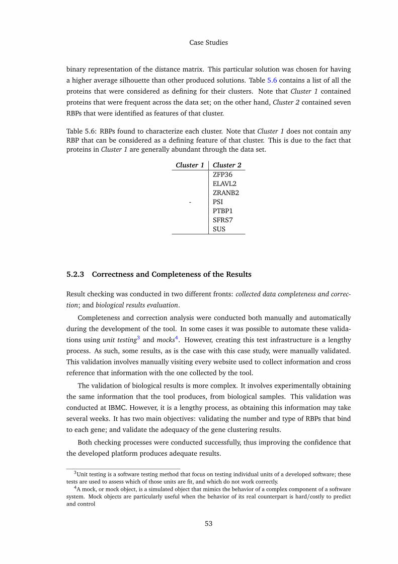
Case Studies
binary representation of the distance matrix. This particular solution was chosen for having
a higher average silhouette than other produced solutions. Table 5.6 contains a list of all the
proteins that were considered as defining for their clusters. Note that Cluster 1 contained
proteins that were frequent across the data set; on the other hand, Cluster 2 contained seven
RBPs that were identified as features of that cluster.
Table 5.6: RBPs found to characterize each cluster. Note that Cluster 1 does not contain anyRBP that can be considered as a defining feature of that cluster. This is due to the fact thatproteins in Cluster 1 are generally abundant through the data set.
Cluster 1 Cluster 2
-
ZFP36ELAVL2ZRANB2PSIPTBP1SFRS7SUS
5.2.3 Correctness and Completeness of the Results
Result checking was conducted in two different fronts: collected data completeness and correc-
tion; and biological results evaluation.
Completeness and correction analysis were conducted both manually and automatically
during the development of the tool. In some cases it was possible to automate these valida-
tions using unit testing3 and mocks4. However, creating this test infrastructure is a lengthy
process. As such, some results, as is the case with this case study, were manually validated.
This validation involves manually visiting every website used to collect information and cross
reference that information with the one collected by the tool.
The validation of biological results is more complex. It involves experimentally obtaining
the same information that the tool produces, from biological samples. This validation was
conducted at IBMC. However, it is a lengthy process, as obtaining this information may take
several weeks. It has two main objectives: validating the number and type of RBPs that bind
to each gene; and validate the adequacy of the gene clustering results.
Both checking processes were conducted successfully, thus improving the confidence that
the developed platform produces adequate results.
3Unit testing is a software testing method that focus on testing individual units of a developed software; thesetests are used to assess which of those units are fit, and which do not work correctly.
4A mock, or mock object, is a simulated object that mimics the behavior of a complex component of a softwaresystem. Mock objects are particularly useful when the behavior of its real counterpart is hard/costly to predictand control
53

Case Studies
5.2.4 Comparison with Previous Method
As with any newly developed automation tool, it is essential to assess if the developed tool is
in fact an improvement over previously available methods. The results produced by the tool
were already determined correct in Section 5.2.3. As such, the tool should now be evaluated
from the user experience standpoint, namely, in terms of task simplification and efficiency.
Task Simplification
Figure 5.1 depicts how PBS Finder simplified the analysis process, from the user point of view.
When conducting a manual analysis, the user must individually analyse every gene in the data
set.
The first step is to select a gene for analysis. The gene identifier is then searched in either
Ensembl or NCBI web platforms, depending on the type of the identifier. If the gene is found
in those platforms, the next step involves finding the 3’UTR sequence in the results page and
copying it. That sequence is then passed to an online RBP analysis platform, that should
retrieve a list of RBPs that may bind to that particular sequence. Lastly, the RBP information
must be manually combined in the results table. When this information is collected for every
gene it is finally possible to conduct a useful analysis.
On the other hand, with PBS Finder the user needs only to provide the complete list of
all gene identifiers in the data set. The tool will them automatically process those identifiers,
find all relevant information and present it to the user, ready for further analysis. Note that
these results contain additional information that is not available in the manual analysis: gene,
transcript and protein information (names, additional sequences, pathways, etc.); links to
external platforms; useful histograms; and gene and protein clustering results.
Efficiency
It is essential for the developed platform to be able to conduct the analysis in a timely fashion,
making tool performance a major concern. As such, we compared the average time that an
expert would take to analyse the data set to the average time that the tool takes to analyse
the same data set.
The consulted molecular biology expert estimated that, on average, it would take thirty
minutes to analyse a single gene. This means that an expert would need an average of eleven
and a half hours (30 minutes×23 genes) to process the entire case study data set.
On the other hand, the automated tool takes a shorter amount of time to conduct the
analysis of the same data set. In order to assess the actual amount of time the tool took to
analyse the entire data set we ran twenty sequential experiences, ten for each of the exper-
imental environments. Table 5.7 depicts the duration of each one of those experiments, as
well as their average duration. As expected, an automated tool widely outperforms a human
expert in information collection and analysis.
54

Case Studies
(a) Manual Analysis (b) Automatic Analysis (PBS Finder)
Microarray or RNA-Seq gene list Microarray or RNA-Seq gene list
Select a gene
Search for the mRNA sequence(NCBI or Ensembl web platforms)
Select the 3’UTR sequence
Search for the 3’UTR sequence
in a RBP Database
Fill in the gene/RBP table
Analyse the results
Copy IDs into PBS Finder
Analyse the results
Candidate selection Candidate selection
Repeat for
each gene
Figure 5.1: Comparison between manual RBP analysis and automatic RBP analysis (conductedwith PBS Finder).
Table 5.8 contains the stress test results of both machines, compared to the estimated
work time needed by an expert. In this case stress tests were executed with one hundred,
five hundred and nine hundred gene identifiers. Even the slowest test can be completed by
the machine with less performance (Machine2) in under three hours. That same effort would
take an expert approximately four hundred and fifty hours, which amounts to two and a half
weeks on a twenty four hour working day, and to just under two months in normal working
conditions (eight hours per day).
55

Case Studies
Table 5.7: Execution times of the case study data set in two different environments (sequentialexperiments). Note that while Machine2 has a significant loss in performance (due to itsoutdated hardware) it still achieves satisfactory execution times. This test also shows that itis possible to efficiently run PBS Finder in a home computer.
Machine1 Machine2Experience 1 1m 47s 6m 34sExperience 2 1m 58s 6m 25sExperience 3 1m 46s 6m 30sExperience 4 1m 45s 6m 15sExperience 5 2m 23s 6m 42sExperience 6 1m 35s 6m 30sExperience 7 1m 40s 6m 31sExperience 8 1m 39s 6m 11sExperience 9 1m 42s 6m 42sExperience 10 1m 42s 6m 52sAverage time 1m 42s 6m 31s
Table 5.8: Results comparison between manual analysis and both test machines.
Number of IDs Machine1 Machine2 Manual method100 9m 56s 11m 1s ≈ 50h500 41m 47s 55m 51s ≈ 250h900 1h 33m 32s 2h 7m 4s ≈ 450h
5.3 Chapter Conclusions
The first case study has shown that the developed tool for result combination can in fact
produce more refined data sets. These filtered and combined data sets eliminate unnecessary
data, and give biologists an higher level of confidence in the differential expression results.
Through the second case study we have shown that PBS Finder produces relevant and
correct results for large-scale analysis of RBPs using data from NGS techniques. We have also
shown that our tool significantly facilitates the work of the biologist, by making analysis of
this data easier and quicker. As such, we consider PBS Finder a tool of great value for studying
RNA biology.
56

Chapter 6
Conclusions
In this thesis we developed a prototype of an integrated platform for RNA-Seq data analysis.
This platform is able to perform the entire analysis process, from the sequencing reads, to
grouping genes by their RBPs. This means that is able to perform read alignment, quantifica-
tion and differential expression analysis tasks, as well as data set enrichment, RBP identifica-
tion and clustering analysis of genes and proteins. Through two case studies we showed the
developed prototype in use, and assessed its correctness and efficiency. Below we will share
our thoughts on the fulfilment of the objectives of this thesis, and present some possibilities
for any future development in our solution.
During this thesis we were advised by molecular biology experts from IBMC. The data set
used in the second case study was provided by IBMC experts and the results obtained are
currently being experimentally verified in their laboratory.
6.1 Objective Fulfilment
Our objectives, in terms of studying the problem at hand and developing a solution to it,
were completely fulfilled. The proposed solution corresponds to all of our expectations. Both
analysis pipelines were completely prototyped and tested, being that PBS Finder was tested in
both development and production environments. However, it was not possible to integrate the
RNA-seq data analysis pipeline with PBS Finder’s analysis pipeline, due to time constraints.
Similarly, it was also not possible to provide the RNA-Seq analysis pipeline’s functionality
through the web interface. As such, our objective of prototyping and testing the complete
integrated system could not be completely achieved.
57
Conclusions
6.2 Future Work
A natural continuation of the proposed work would be to finish the implementation and in-
tegration of the RNA-Seq data analysis pipeline. This would allow our solution to work as
designed, integrating the complete analysis pipeline, from sequencing data to gene cluster-
ing and result visualization. Furthermore, it would be useful to study the developed tools in
terms of performance, under large volumes of information and requests. Whilst the tools were
developed taking in consideration their performance, making them available in a large scale
would require another kind of infrastructure.
58

References
[AH10] Simon Anders and Wolfgang Huber. Differential expression analysis for se-quence count data. Genome Biology, 11(10):R106, 2010.
[APH14] Simon Anders, Paul Theodor Pyl, and Wolfgang Huber. Htseq – apython framework to work with high-throughput sequencing data. bioRxiv,2014.
[Bla03] Douglas L. Black. Mechanisms of alternative pre-messenger rna splicing.Annual Review of Biochemistry, 72(1):291–336, 2003. PMID: 12626338.
[BM95] Ivan Bratko and Stephen Muggleton. Applications of Inductive Logic Pro-gramming. Commun. ACM, 38(11):65–70, November 1995.
[CDR11] Vítor S. Costa, Luís Damas, and Ricardo Rocha. The YAP Prolog System.February 2011.
[CEF+12] Soumen Chakrabarti, Martin Ester, Usama Fayyad, Johannes Gehrke, JiaweiHan, Shinichi Morishita, Gregory Piatetsky-Shapiro, and Wei Wang. Datamining curriculum: a proposal, version 1.0. Available at www.kdd.org/curriculum/CURMay06.pdf, last access on February 2014, April 2012.
[CFG+10] Peter J a Cock, Christopher J Fields, Naohisa Goto, Michael L Heuer, and Pe-ter M Rice. The Sanger FASTQ file format for sequences with quality scores,and the Solexa/Illumina FASTQ variants. Nucleic acids research, 38(6):1767–71, April 2010.
[CKZ+11] Kate B. Cook, Hilal Kazan, Khalid Zuberi, Quaid Morris, and Timothy R.Hughes. Rbpdb: a database of rna-binding specificities. Nucleic Acids Re-search, 39(suppl 1):D301–D308, 2011.
[CWD09] Thomas A Cooper, Lili Wan, and Gideon Dreyfuss. {RNA} and Disease. Cell,136(4):777–793, March 2009.
[EpKSX96] Martin Ester, Hans peter Kriegel, Jörg S, and Xiaowei Xu. A density-basedalgorithm for discovering clusters in large spatial databases with noise. pages226–231. AAAI Press, 1996.
[FA05] John Fox and Robert Andersen. Using the R statistical computing environ-ment to teach social statistics courses. Department of Sociology, McMasterUniversity, (January), 2005.
59

REFERENCES
[Fas12] Joe Fass. Read alignment for RNA-Seq. Bioinformatics Core, University ofCalifornia, available at http://training.bioinformatics.ucdavis.edu/docs/2012/05/RNA/_downloads/Alignment.pdf, May 2012.
[FCC12] Nuno A Fonseca, Vítor Santos Costa, and Rui Camacho. Conceptual cluster-ing of multi-relational data. In Inductive Logic Programming, pages 145–159.Springer, 2012.
[FCSC03] Nuno Fonseca, VS Vitor Santos Costa, Fernando Silva, and Rui Camacho. Onthe implementation of an ILP system with Prolog. Technical report, Technicalreport, DCC-FC & LIACC, UP, 2003.
[FEB+11] Nuno Fonseca, Dent Earl, Keith Bradnam, et al. Assemblathon 1: A compet-itive assessment of de novo short read assembly methods. Genome Research,21(12):2224–2241, December 2011.
[FJ05] Stanley Fields and Mark Johnston. Cell biology: Whither model organismresearch? Science, 307(5717):1885–1886, 2005.
[FPMB14] Nuno A. Fonseca, Robert Petryszak, John Marioni, and Alvis Brazma. irap -an integrated rna-seq analysis pipeline. bioRxiv, 2014.
[FPSS96] UM Fayyad, G Piatetsky-Shapiro, and P Smyth. Knowledge Discovery andData Mining: Towards a Unifying Framework. KDD, 1996.
[GEN] GENIE. Gene expression and regulation. University of Leicester,available at http://www2.le.ac.uk/departments/genetics/vgec/schoolscolleges/topics/geneexpression-regulation, last ac-cess on February 2014.
[Goo] Steven Goodman. A dirty dozen: Twelve p-value misconceptions. SeminHematol, 45:135–140.
[HKP06] Jiawei Han, Micheline Kamber, and Jian Pei. Data mining: concepts andtechniques. Morgan kaufmann, 2006.
[HNF+09] Mark Hall, Hazeltine National, Eibe Frank, Geoffrey Holmes, BernhardPfahringer, Peter Reutemann, and Ian H Witten. The WEKA Data MiningSoftware : An Update. SIGKDD Explorations, 11(1):10–18, 2009.
[Iha98] Ross Ihaka. R: Past and future history. COMPUTING SCIENCE AND STATIS-TICS, 1998.
[JEF11] Simon Jupp, James Eales, and Simon Fischer. Combining RapidMiner op-erators with bioinformatics services–a powerful combination. In RapidMinerCommunity Meeting and Conference, (RCOMM), 2011.
[JM11] Sarath Chandra Janga and Nitish Mittal. Construction, structure and dynam-ics of post-transcriptional regulatory network directed by RNA-binding pro-teins. In RNA Infrastructure and Networks, pages 103–117. Springer, 2011.
[Lab] Abecasis Lab. Sam - genome analysis wiki. University of Michigan, availableat http://genome.sph.umich.edu/wiki/SAM, last access on February2014.
60

REFERENCES
[LBZ00] Harvey Lodish, Arnold Berk, and SL Zipursky. Molecular cell biology 4thedition. 2000.
[LD98] N Lavrac and S Dzeroski. Inductive logic programming, volume 1446 of Lec-ture Notes in Computer Science. Springer-Verlag, Berlin/Heidelberg, 1998.
[Lei02] Friedrich Leisch. Sweave: Dynamic generation of statistical reports usingliterate data analysis. In Wolfgang Härdle and Bernd Rönz, editors, Comp-stat 2002 — Proceedings in Computational Statistics, pages 575–580. PhysicaVerlag, Heidelberg, 2002. ISBN 3-7908-1517-9.
[LHW+09] Heng Li, Bob Handsaker, Alec Wysoker, Tim Fennell, Jue Ruan, Nils Homer,Gabor Marth, Goncalo Abecasis, and Richard Durbin. The SequenceAlignment/Map format and SAMtools. Bioinformatics (Oxford, England),25(16):2078–9, August 2009.
[LTP+09] Ben Langmead, Cole Trapnell, Mihai Pop, Steven L Salzberg, et al. Ultra-fast and memory-efficient alignment of short dna sequences to the humangenome. Genome Biol, 10(3):R25, 2009.
[Lyo98] Robert Lyons. A molecular biology glossary. DNA Sequencing Core, Univer-sity of Michigan, available at http://seqcore.brcf.med.umich.edu/doc/educ/dnapr/mbglossary/mbgloss.html, last access on February2014, July 1998.
[Mad12] T. Soni Madhulatha. An overview on clustering methods. CoRR,abs/1205.1117, 2012.
[MCYS09] Uma Mudunuri, Anney Che, Ming Yi, and Robert M. Stephens. biodbnet: thebiological database network. Bioinformatics, 25(4):555–556, 2009.
[MMNMMN13] Michaela Muller-McNicoll, Karla M Neugebauer, Michaela Müller-McNicoll,and Karla M Neugebauer. How cells get the message: dynamic assembly andfunction of mRNA-protein complexes. Nat Rev Genet, 14(4):275–287, April2013.
[MRS08] Christopher D. Manning, Prabhakar Raghavan, and Hinrich Schütze. Intro-duction to Information Retrieval. Cambridge University Press, New York, NY,USA, 2008.
[Mug91] Stephen Muggleton. Inductive logic programming. New Generation Comput-ing, 8(4):295–318, 1991.
[MW11] Jeffrey Martin and Zhong Wang. Next-generation transcriptome assembly.Nature reviews. Genetics, 12(10):671–82, October 2011.
[NCB] NCBI. Web blast page options. NCBI, available at https://www.ncbi.nlm.nih.gov/BLAST/blastcgihelp.shtml, last access on February2014.
[PASH03] Lajos Pusztai, Mark Ayers, James Stec, and Gabriel N Hortobágyi. ClinicalApplication of cDNA Microarrays in Oncology. The Oncologist, 8(3):252–258,January 2003.
61

REFERENCES
[rap12] RapidMiner. Available at http://rapid-i.com/content/view/181/190/, last access on May 2014, April 2012.
[RF09] Jorge S. Reis-Filho. Next-generation sequencing. Breast cancer research :BCR, 11 Suppl 3:S12, January 2009.
[RMS10] M.D. Robinson, D.J. McCarthy, and G.K. Smyth. edger: a bioconductor pack-age for differential expression analysis of digital gene expression data. Bioin-formatics, 26(1):139–140, 2010.
[Rou87] Peter J. Rousseeuw. Silhouettes: A graphical aid to the interpretation andvalidation of cluster analysis. Journal of Computational and Applied Mathe-matics, 20(0):53 – 65, 1987.
[San11] Sanger Institute. Gff (general feature format). Available at http://www.sanger.ac.uk/resources/software/gff/spec.html, last access onFebruary 2014, 2011.
[SH07] Nahum Sonenberg and Alan G Hinnebusch. New Modes of TranslationalControl in Development, Behavior, and Disease. Molecular Cell, 28(5):721–729, December 2007.
[SH09] Nahum Sonenberg and Alan G Hinnebusch. Regulation of Translation Initi-ation in Eukaryotes: Mechanisms and Biological Targets. Cell, 136(4):731–745, February 2009.
[Smi13] Smith, Steven and Browning, Brian. Introduction to variant call format.Available at http://faculty.washington.edu/browning/beagle/intro-to-vcf.html, last access on February 2014, 2013.
[SSK11] Christof Strauch, Ultra-Large Scale Sites, and Walter Kriha. Nosql databases.Lecture Notes, Stuttgart Media University, 2011.
[TPS09] Cole Trapnell, Lior Pachter, and Steven L. Salzberg. Tophat: discoveringsplice junctions with rna-seq. Bioinformatics, 25(9):1105–1111, 2009.
[TWP+10] Cole Trapnell, Brian A Williams, Geo Pertea, Ali Mortazavi, Gordon Kwan,Marijke J van Baren, Steven L Salzberg, Barbara J Wold, and Lior Pachter.Transcript assembly and quantification by rna-seq reveals unannotated tran-scripts and isoform switching during cell differentiation. Nature biotechnol-ogy, 28(5):511–515, 2010.
[VNN13] Leif Väremo, Jens Nielsen, and Intawat Nookaew. Enriching the gene setanalysis of genome-wide data by incorporating directionality of gene ex-pression and combining statistical hypotheses and methods. Nucleic AcidsResearch, 41(8):4378–4391, 2013.
[WL09] Brian T Wilhelm and Josette-Renée Landry. RNA-Seq-quantitative measure-ment of expression through massively parallel RNA-sequencing. Methods(San Diego, Calif.), 48(3):249–57, July 2009.
[Wol13] Jochen B W Wolf. Principles of transcriptome analysis and gene expressionquantification: an RNA-seq tutorial. Molecular ecology resources, 13(4):559–72, July 2013.
62

Glossary
Alternative splicing
Alternative splicing that causes a specific gene to be transcribed to several different RNA
sequences, by means of different combinations of exons. This process is a major source
of protein diversity in an organism [Bla03].
cDNA
DNA which has been reverse transcribed using RNA as a template [Lyo98].
Cytoplasm
The protoplasm of a cell contained within the cell membrane, but excluding the nucleus.
It helps to move materials around the cell and is also responsible for dissolving cellular
waste [Lyo98].
Exon
The portions of a genomic DNA sequence which will be represented in the final, ma-
ture mRNA. Exons may include coding sequences, the 5’ untranslated region or the 3’
untranslated region [Lyo98].
Expression
To “express” a gene is to cause it to function. A gene which encodes a protein will, when
expressed, be transcribed and translated to produce that protein. A gene which encodes
an RNA rather than a protein (for example, a rRNA gene) will produce that RNA when
expressed [Lyo98].
Gene
A unit of DNA which performs one function. Usually, this is equated with the produc-
tion of one RNA or one protein. A gene contains coding regions, introns, untranslated
regions and control regions [Lyo98].
Genome
The total DNA contained in each cell of an organism. There are somewhere in the order
of a hundred thousand genes, including coding regions, 5’ and 3’ untranslated regions,
introns, 5’ and 3’ flanking DNA [Lyo98].
63

Glossary
Intron
Introns are portions of genomic DNA which are transcribed (and thus present in the
primary transcript) but which are later spliced out. Thus, they are not present in the
mature mRNA [Lyo98].
mRNA
“Messenger RNA” contains sequences coding for a protein. The term mRNA is used only
for a mature transcript (with all introns removed), rather than the primary transcript in
the nucleus [Lyo98].
Nucleus
The nucleus is a part of the cell, that is enclosed by a membrane [Lyo98]. It contains
the cell’s genetic information, in the form of DNA and RNA molecules [Lyo98].
rRNA
“Ribosomal RNA” describes any of several RNAs which become part of the ribosome,
and thus are involved in translating mRNA and synthesizing proteins [Lyo98].
Shotgun cloning
The process of randomly shearing an organism’s genomic DNA and cloning it into a
suitable vector, resulting in a genomic library [Lyo98].
Shotgun sequencing
Sequencing the DNA library created by shotgun cloning [Lyo98].
Signal transduction
Process in which an extracellular signaling molecule activates a specific receptor located
in the border (or inside) a cell; in turn this receptor triggers a chain of events inside the
cell that leads to its response [LBZ00].
Transcription
The process of copying DNA to produce an RNA transcript. This is the first step in the
expression of any gene. The resulting RNA will produce the desired protein molecule
by the process of translation [Lyo98].
Translation
The process of decoding a strand of mRNA, thereby producing a protein based on the
code [Lyo98].
64

Glossary
tRNA
“Transfer RNA” represents one of a class of rather small RNAs used by the cell to carry
amino acids to the enzyme complex (the ribosome) which builds proteins, using an
mRNA as a guide [Lyo98].
65

Glossary
66
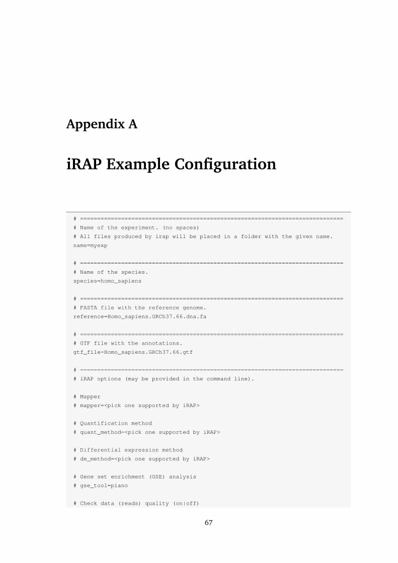
Appendix A
iRAP Example Configuration
# =============================================================================
# Name of the experiment. (no spaces)
# All files produced by irap will be placed in a folder with the given name.
name=myexp
# =============================================================================
# Name of the species.
species=homo_sapiens
# =============================================================================
# FASTA file with the reference genome.
reference=Homo_sapiens.GRCh37.66.dna.fa
# =============================================================================
# GTF file with the annotations.
gtf_file=Homo_sapiens.GRCh37.66.gtf
# =============================================================================
# iRAP options (may be provided in the command line).
# Mapper
# mapper=<pick one supported by iRAP>
# Quantification method
# quant_method=<pick one supported by iRAP>
# Differential expression method
# de_method=<pick one supported by iRAP>
# Gene set enrichment (GSE) analysis
# gse_tool=piano
# Check data (reads) quality (on|off)
67
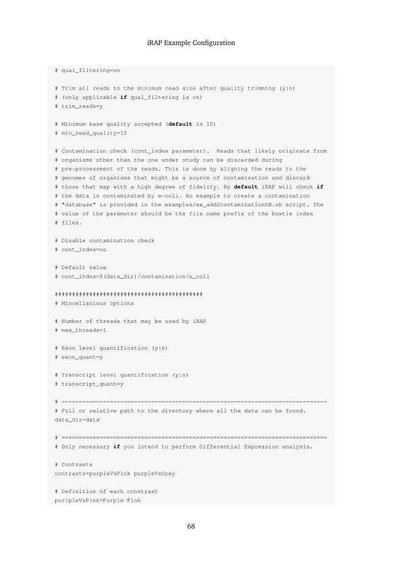
iRAP Example Configuration
# qual_filtering=on
# Trim all reads to the minimum read size after quality trimming (y|n)
# (only applicable if qual_filtering is on)
# trim_reads=y
# Minimum base quality accepted (default is 10)
# min_read_quality=10
# Contamination check (cont_index parameter). Reads that likely originate from
# organisms other than the one under study can be discarded during
# pre-processment of the reads. This is done by aligning the reads to the
# genomes of organisms that might be a source of contamination and discard
# those that map with a high degree of fidelity. By default iRAP will check if
# the data is contaminated by e-coli. An example to create a contamination
# "database" is provided in the examples/ex_add2contaminationDB.sh script. The
# value of the parameter should be the file name prefix of the bowtie index
# files.
# Disable contamination check
# cont_index=no
# Default value
# cont_index=$(data_dir)/contamination/e_coli
###########################################
# Miscellanious options
# Number of threads that may be used by iRAP
# max_threads=1
# Exon level quantification (y|n)
# exon_quant=y
# Transcript level quantification (y|n)
# transcript_quant=y
# =============================================================================
# Full or relative path to the directory where all the data can be found.
data_dir=data
# =============================================================================
# Only necessary if you intend to perform Differential Expression analysis.
# Contrasts
contrasts=purpleVsPink purpleVsGrey
# Definition of each constrast
purlpleVsPink=Purple Pink
68

iRAP Example Configuration
purlpleVsGrey=Purple Grey
# Groups definition
Purlple=myLib1 myLib2
Pink=myLib3
Grey=myLib4
# Technical replicates
technical.replicates="myLib1,myLib2;myLib3;mylib4"
# =============================================================================
# Data
# *_rs => read size
# *_qual => quality encoding (33|64)
# *_sd => standard deviation
# *_ins => insert size
myLib1=f1.fastq
myLib1_rs=75
myLib1_qual=33
myLib2=f2.fastq
myLib2_rs=75
myLib2_qual=33
myLib3=f3_1.fastq f3_2.fastq
myLib3_rs=50
myLib3_qual=33
myLib3_ins=350
myLib3_sd=60
myLib4=f4_1.fastq f4_2.fastq
myLib4_rs=50
myLib4_qual=33
myLib4_ins=350
myLib4_sd=60
# List the names of your single-end (se) and paired (pe) libraries
se=myLib1 myLib2
pe=myLib3 myLib4
69

iRAP Example Configuration
70

Appendix B
Examples of Biological Information
Files
B.1 SAM Example
HD VN:1.0 SO:coordinate
@SQ SN:seq1 LN:5000
@SQ SN:seq2 LN:5000
@CO Example of SAM/BAM file format.
B7_591:4:96:693:509 73 seq1 1 99 36M * 0 0
CACTAGTGGCTCATTGTAAATGTGTGGTTTAACTCG <<<<<<<<<<<<<<<;<<<<<<<<<5<<<<<;:<;7
MF:i:18 Aq:i:73 NM:i:0 UQ:i:0 H0:i:1 H1:i:0
EAS54_65:7:152:368:113 73 seq1 3 99 35M * 0 0
CTAGTGGCTCATTGTAAATGTGTGGTTTAACTCGT <<<<<<<<<<0<<<<655<<7<<<:9<<3/:<6): MF:i
:18 Aq:i:66 NM:i:0 UQ:i:0 H0:i:1 H1:i:0
EAS51_64:8:5:734:57 137 seq1 5 99 35M * 0 0 AGTGGCTCATTGTAAATGTGTGGTTTAACTCGTCC
<<<<<<<<<<<7;71<<;<;;<7;<<3;);3*8/5 MF:i:18 Aq:i:66 NM:i:0 UQ:i:0 H0:i:1
H1:i:0
B7_591:1:289:587:906 137 seq1 6 63 36M * 0 0
GTGGCTCATTGTAATTTTTTGTTTTAACTCTTCTCT (-&----,----)-)-),’--)---’,+-,),’’*,
MF:i:130 Aq:i:63 NM:i:5 UQ:i:38 H0:i:0 H1:i:0
EAS56_59:8:38:671:758 137 seq1 9 99 35M * 0 0
GCTCATTGTAAATGTGTGGTTTAACTCGTCCATGG <<<<<<<<<<<<<<<;<;7<<<<<<<<7<<;:<5% MF:i
:18 Aq:i:72 NM:i:0 UQ:i:0 H0:i:1 H1:i:0
EAS56_61:6:18:467:281 73 seq1 13 99 35M * 0 0
ATTGTAAATGTGTGGTTTAACTCGTCCCTGGCCCA <<<<<<<<;<<<8<<<<<;8:;6/686&;(16666 MF:i
:18 Aq:i:39 NM:i:1 UQ:i:5 H0:i:0 H1:i:1
EAS114_28:5:296:340:699 137 seq1 13 99 36M * 0 0
ATTGTAAATGTGTGGTTTAACTCGTCCATGGCCCAG <<<<<;<<<;<;<<<<<<<<<<<8<8<3<8;<;<0;
MF:i:18 Aq:i:73 NM:i:0 UQ:i:0 H0:i:1 H1:i:0
71

Examples of Biological Information Files
B.2 VCF Example
##fileformat=VCFv4.0
##fileDate=20090805
##source=myImputationProgramV3.1
##reference=1000GenomesPilot-NCBI36
##phasing=partial
##INFO=<ID=NS,Number=1,Type=Integer,Description="Number of Samples With Data">
##INFO=<ID=DP,Number=1,Type=Integer,Description="Total Depth">
##INFO=<ID=AF,Number=.,Type=Float,Description="Allele Frequency">
##INFO=<ID=AA,Number=1,Type=String,Description="Ancestral Allele">
##INFO=<ID=DB,Number=0,Type=Flag,Description="dbSNP membership, build 129">
##INFO=<ID=H2,Number=0,Type=Flag,Description="HapMap2 membership">
##FILTER=<ID=q10,Description="Quality below 10">
##FILTER=<ID=s50,Description="Less than 50% of samples have data">
##FORMAT=<ID=GT,Number=1,Type=String,Description="Genotype">
##FORMAT=<ID=GQ,Number=1,Type=Integer,Description="Genotype Quality">
##FORMAT=<ID=DP,Number=1,Type=Integer,Description="Read Depth">
##FORMAT=<ID=HQ,Number=2,Type=Integer,Description="Haplotype Quality">
#CHROM POS ID REF ALT QUAL FILTER INFO
FORMAT NA00001 NA00002
NA00003
20 14370 rs6054257 G A 29 PASS NS=3;DP=14;AF=0.5;DB;H2
GT:GQ:DP:HQ 0|0:48:1:51,51 1|0:48:8:51,51 1/1:43:5:.,.
20 17330 . T A 3 q10 NS=3;DP=11;AF=0.017
GT:GQ:DP:HQ 0|0:49:3:58,50 0|1:3:5:65,3 0/0:41:3
20 1110696 rs6040355 A G,T 67 PASS NS=2;DP=10;AF=0.333,0.667;AA=
T;DB GT:GQ:DP:HQ 1|2:21:6:23,27 2|1:2:0:18,2 2/2:35:4
20 1230237 . T . 47 PASS NS=3;DP=13;AA=T
GT:GQ:DP:HQ 0|0:54:7:56,60 0|0:48:4:51,51 0/0:61:2
20 1234567 microsat1 GTCT G,GTACT 50 PASS NS=3;DP=9;AA=G
GT:GQ:DP 0/1:35:4
B.3 FASTQ Example
@SRR014849.1 EIXKN4201CFU84 length=93
GGGGGGGGGGGGGGGGCTTTTTTTGTTTGGAACCGAAAGG
GTTTTGAATTTCAAACCCTTTTCGGTTTCCAACCTTCCAA
AGCAATGCCAATA
+SRR014849.1 EIXKN4201CFU84 length=93
3+&$#"""""""""""7F@71,’";C?,B;?6B;:EA1EA
1EA5’9B:?:#9EA0D@2EA5’:>5?:%A;A8A;?9B;D@
/=<?7=9<2A8==
72

Examples of Biological Information Files
B.4 FASTA Example
>gi|5524211|gb|AAD44166.1| cytochrome b [Elephas maximus maximus]
LCLYTHIGRNIYYGSYLYSETWNTGIMLLLITMATAFMGYVLPWGQMSFWGATVITNLFSAIPYIGTNLV
EWIWGGFSVDKATLNRFFAFHFILPFTMVALAGVHLTFLHETGSNNPLGLTSDSDKIPFHPYYTIKDFLG
LLILILLLLLLALLSPDMLGDPDNHMPADPLNTPLHIKPEWYFLFAYAILRSVPNKLGGVLALFLSIVIL
GLMPFLHTSKHRSMMLRPLSQALFWTLTMDLLTLTWIGSQPVEYPYTIIGQMASILYFSIILAFLPIAGX
IENY
B.5 GTF/GFF Example
## GFF
##gff-version 3
##sequence-region ctg123 1 1497228
ctg123 . gene 1000 9000 . + . ID=gene00001;Name=EDEN
ctg123 . TF_binding_site 1000 1012 . + . ID=tfbs00001;Parent=gene00001
ctg123 . mRNA 1050 9000 . + . ID=mRNA00001;Parent=gene00001;Name=
EDEN.1
ctg123 . mRNA 1050 9000 . + . ID=mRNA00002;Parent=gene00001;Name=
EDEN.2
ctg123 . mRNA 1300 9000 . + . ID=mRNA00003;Parent=gene00001;Name=
EDEN.3
ctg123 . exon 1300 1500 . + . ID=exon00001;Parent=mRNA00003
ctg123 . exon 1050 1500 . + . ID=exon00002;Parent=mRNA00001,
mRNA00002
ctg123 . exon 3000 3902 . + . ID=exon00003;Parent=mRNA00001,
mRNA00003
---------------------------------------------------
## GTF
140 Twinscan inter 5141 8522 . - . gene_id "";
transcript_id "";
140 Twinscan inter_CNS 8523 9711 . - . gene_id "";
transcript_id "";
140 Twinscan inter 9712 13182 . - . gene_id "";
transcript_id "";
140 Twinscan 3UTR 65149 65487 . - . gene_id "
140.000"; transcript_id "140.000.1";
140 Twinscan 3UTR 66823 66992 . - . gene_id "
140.000"; transcript_id "140.000.1";
140 Twinscan stop_codon 66993 66995 . - 0 gene_id "
140.000"; transcript_id "140.000.1";
73