A Computational Study of the Aerodynamics and

Aeroacoustics of a Flatback Airfoil Using Hybrid

RANS-LES

Christopher Stone∗

Computational Science & Engineering, Athens, GA, 30606, USA

Matthew Barone†

Sandia National Laboratories, Albuquerque, NM, 87185-1124, USA

C. Eric Lynch‡ and Marilyn J. Smith§

Georgia Institute of Technology, Atlanta, Georgia, 30332-0150, USA

This work compares the aerodynamic and aeroacoustic predictions for flatback air-foil geometries obtained by applying advanced turbulence modeling simulation techniqueswithin Computational Fluid Dynamics (CFD) methods that resolve the Reynolds-AveragedNavier-Stokes (RANS) equations of motion. These flatback airfoil geometries are designedfor wind turbine applications. Results from different CFD codes using hybrid RANS-LESand RANS turbulence simulations are correlated and include analysis with experimentaldata. These data comparisons include aerodynamic and a limited amount of aeroacousticresults. While the mean lift prediction remains relatively insensitive across many simulationtechniques and parameters, the mean drag prediction is dependent on both the grid andturbulence simulation method. Aeroacoustic predictions obtained from post-processing ofthe airfoil surface pressure agree reasonably well with experimental data when consistentboundary layer tripping is used for both the simulation and experimental configuration.

Nomenclature

a Speed of soundc Chord, mCd Sectional drag coefficientCD Total drag coefficientCl Sectional lift coefficientCL Total lift coefficientcp Specific heat due to constant pressureCp Pressure coefficientd Distance to the walle Specific internal energyf Frequency of vortex shedding, 1/sh Base length of the flatback airfoil trailing edge, m or enthalpyi, j, k Unit vectors in the x,y,z directions

∗President and Chief Scientist, AIAA Member.†Senior Member of Technical Staff, Wind Energy Technology Dept., AIAA Senior Member.‡Ph.D. Student and Graduate Research Assistant, School of Aerospace Engineering, AIAA Student Member.§Associate Professor, School of Aerospace Engineering, AIAA Associate Fellow.

1

47th AIAA Aerospace Sciences Meeting Including The New Horizons Forum and Aerospace Exposition5 - 8 January 2009, Orlando, Florida

AIAA 2009-273

This material is declared a work of the U.S. Government and is not subject to copyright protection in the United States.

k Turbulent kinetic energyl LengthM Mach numberN Number of grid pointsp PressurePrL Laminar Prandtl number, PrL = cpµ/κq Heat flux vectorR Distance from sound source to observer, mRLL Lift fluctuation correlation functionRe Reynolds numberSt Strouhal number, St = fh/U∞

t Time, sT Temperatureu, v, w Velocity in the x, y, z directionsx, y, z Cartesian coordinate system in the stream, normal and span directionsZ Spanwise extent of the computational domainy+ Dimensionless sublayer-scaled distance, uT y/νU Velocityα Angle of attack, degrees ()∆ Local grid cell size or change in quantityλ Acoustic wavelengthµ Molecular viscosityµT Eddy viscosityΛ Spanwise lift correlation lengthω vorticityρ Densityσ centroid of correlation functionτij Reynolds shear stress tensorθ Angle, as defined in textω Vorticity

Subscripts and Superscripts

i, j, k Tensor directionsl Lengthrms Root mean squaresgs Subgrid-scaletot TotalT Turbulent(.)′ Fluctuating term for a time-averaged quantity(.)′′ Fluctuating term for a Favre-averaged quantity

(.) Mean quantity

(.) Mass-averaged quantity∞ Free stream

Abbreviations

CFD Computational Fluid DynamicsDES Detached Eddy SimulationGT–HRLES Georgia Tech hybrid RANS/LES turbulence methodHRLES Hybrid RANS/LESLES Large Eddy SimulationRANS Reynolds-Averaged Navier-Stokes

2

SA Spalart-Allmaras RANS turbulence modelSPL Sound pressure level, dB (ref: 20 × 10−6 Pa)

I. Introduction

A specific barrier to widespread wind turbine deployment, especially in densely populated areas, is thehigh level of flow-generated noise. To ensure that wind energy can attain appreciable deployment in suchareas, aeroacoustic (i.e., aerodynamically generated) noise must be reduced,1–3 while maintaining optimalturbine performance. The achievement of these two technical goals will permit the expansion and newdevelopment of wind power resources in areas near population centers.

The problems of maintaining or improving performance while reducing the aeroacoustic noise cannot betackled as separate goals, as they are inherently coupled. For example, the design of quieter turbines couldpermit higher turbine tip-speeds, which in turn can improve performance. There are many different sourcesof aeroacoustic noise in a full-scale wind turbine configuration, which are driven by the unsteady aerodynamicflow field. For utility-scale wind turbines, (1) turbulent inflow noise, (2) turbulent boundary layer trailingedge noise and (3) blunt trailing edge vortex shedding noise are the primary sources of aerodynamic noise.Turbulent inflow noise is due to turbulent flow/leading-edge interaction, while turbulent boundary layertrailing edge noise is due to scattering of fluctuations in the turbulent boundary layer by the trailing edge.Blunt trailing edge vortex is a narrow-band noise source that results from organized shedding of vorticity inthe wake of a blunt trailing edge. It is clear that accurate characterization of the local unsteady aerodynamicflow field is key to predicting, understanding, and ultimately reducing the aeroacoustic noise.

With respect to the performance goals, it is well known that the power generating potential of a giventurbine increases proportionately with the rotor disk area. To this end, designers have been investigatingnew wind turbine configurations with ever longer blades. To reduce the overall rotor weight and the resultingdrive-train stress associated with these longer blades, light-weight, composite airfoils are being deployed. Tomaintain the necessary structural integrity and longevity, airfoils with trailing edges that are significantlythickened or even blunted have been studied.4, 5 The complex, bluff-body nature of these airfoils, commonlyknown as flatback airfoils due to their trailing-edge shape, comes with penalties including increased drag andaeroacoustic noise. Recently, Berg and Zayas6 investigated both the aeroacoustic noise and aerodynamicperformance of a flatback airfoil design in a series of anechoic wind-tunnel experiments. Similar perfor-mance studies of flatback airfoils have also been investigated experimentally and numerically.4, 7 Low-fidelity(potential) aerodynamic models are not adequate to properly predict the strength and location salient aero-dynamic phenomena for these wind-turbine airfoils. Existing empirical estimates8 for the noise generationdo not account for thicknesses greater then 1% of chord, complicating the design of new wind turbines.

Computational fluid dynamic (CFD) modeling of wind turbines is desirable as a design and research toolfor both conventional as well as these flatback airfoils, but it is limited because of the difficulties encounteredin accurately predicting the aerodynamic flow field features (e.g., turbulent inflow, separation) that are keyto the performance and noise predictions. Wind turbines routinely operate at a wide disparity of localReynolds numbers (Re) that can reach values of Re > 107 near the rotor tips. The ratio of the largest-to-smallest turbulence scales is proportional to Re9/2. As a consequence, a fully-resolved simulation (e.g.,Direct Numerical Simulations (DNS)) for design and analysis of wind turbines (or even the airfoils) is notpractical for the foreseeable future, without the aid of massively parallel computational hardware. To reducethe computational costs, attempts are made to statistically model the effects of these turbulent scales, whilenumerically simulating the mean flow field. The turbulence models are tuned utilizing a number of differentclassic test cases, none of which include the unsteady, rotational configurations found in wind turbines. Thistraditional method, CFD or Reynolds Averaged Navier-Stokes (RANS) CFD, applies these empirical modelsto all turbulence length- and time-scales, resulting in a steady-state prediction of the macroscopic flow field.Under specific time-scale conditions, an unsteady solution for the slowest time-scales (URANS) is possible.Despite their wide usage, these models are overly dissipative and are poorly suited for predicting unsteady,separated flow typically encountered at high wind speeds (i.e., high angle-of-attack) and near the rotor

3

hub (bluff-body)9–11 where viscous-induced separation is dominant. Furthermore, due to their steady-statenature, direct acoustic predictions derived from RANS are questionable. These restrictions considerablylimit RANS’s predictive potential for wind turbine design and analysis.

Large-Eddy Simulation (LES) methods are an alternative technique to RANS and DNS. Unlike RANS,LES exactly simulates the larger, energy-containing length scales and reverts to phenomenological/empiricalmodeling only at length-scales smaller then the local grid resolution.12, 13 By directly resolving the mostenergetic eddies in both time and space, LES can capture the unsteadiness found in separated flows morerealistically. However, for LES to be applicable, the grid resolution must be sufficiently refined so thatits scaling cut-off will capture eddies in the inertial sub-range. In this regime, the turbulence statisticsare considered more universal and less dependent on the geometry of the flow.14, 15 Unfortunately, theinertial sub-range requirement makes LES an expensive albeit tractable (with sufficient parallel processing)simulation method.

Unfortunately, the flow around a wind turbine has an extremely high Reynolds number (typically, on theorder of several millions) and is geometrically complex (e.g., rotating turbine with twisted blades). Evenwith the computational savings offered by LES, the effective cost remains far too high for design-level CFDstudies. As a compromise, hybrid modeling approaches combine near-wall RANS models with LES methodswhere the turbulent eddy scale disparities are less severe. This methodology can be implemented in existingLES and RANS codes. Most engineering-based applications typically modify an existing RANS code so thatit will employ the LES model in separated flow regions. One of the first, and most commonly used hybridapproach is Detached-Eddy Simulation (DES).12, 16 In this approach, the Spalart-Allmaras one-equation orκ − ω SST RANS model is used in wall-bounded regions and then transitions to a Smagorinsky17 eddy-viscosity model.

In the remainder of this work, a series of numerical simulations mimics some selected configurationsof the experiments conducted with a flatback version of the DU97-W-300 airfoil reported in.6, 18 Thesenumerical simulations are conducted using different existing RANS CFD codes with two hybrid RANS-LESturbulence simulation methods. These results are correlated with aerodynamic loads (e.g., integrated liftand drag forces) and turbulence statistics in the wake. The simulated turbulence data are used to estimatethe blunt trailing edge vortex-shedding noise and compared to the experimental acoustic measurements ofthe vortex-shedding tone.

II. Hybrid RANS/LES Turbulence Simulation Techniques

Recent research efforts19, 20 indicate that advanced turbulence simulation techniques in the guise of hybridRANS/LES methods show some promise in bridging the gap between RANS and LES computational tech-niques. It has been postulated19 that hybrid techniques in legacy CFD codes should capture the largest scaleswherever grid resolution is sufficient to support LES. Thus even coarse grids, more suitable for Very-Large

LES (VLES), should be more representative of the flow physics than RANS simulations on comparably-sizedgrids.

The compressible Navier-Stokes equations, when Favre-averaged (mass-averaged), can be mathematicallyexpressed as :

4

∂ρ

∂t+

∂

∂xj(ρuj) = 0

∂

∂t(ρui) +

∂

∂xj(ρuiuj) = −

∂p

∂xi+

∂σij

∂xj−

∂

∂xj(ρu

′′

i u′′

j )

∂

∂t[ρ(e + 0.5uiui)] +

∂

∂xj[ρuj(h + 0.5uiui)] =

∂

∂xj(−qLj

+ uiσij) −∂

∂t[0.5ρu′′

i u′′i ]

+∂

∂xj[−ujρu′′

i u′′j + uj0.5ρu′′

i u′′i − ρu′′

j h′′

+ σjiu′′i − 0.5ρu′′

j u′′i u′′

i ]] (1)

As a result of the averaging process, a Reynolds-stress tensor (ρτij = −ρu′′i u′′

i ) appears that requires

closure. The turbulent kinetic energy (k) can then be defined as ρk = 0.5ρu′′i u′′

i . Favre-averaging also

gives rise to the the turbulent heat flux (qT i = ρu′′i h′′) and the rate of turbulent dissipation (ρǫ = σji

∂u′′

i

∂xj).

For flows up through the low supersonic regime, the molecular diffusion and turbulent transport terms(σjiu′′

i − ρu′′j 0.5u′′

i u′′i ) are typically ignored.21

∂ρ

∂t+

∂

∂xj(ρuj) = 0

∂

∂t(ρui) +

∂

∂xj(ρuiuj) = −

∂p

∂xi+

∂σij

∂xj−

∂

∂xj(ρτij)

∂

∂t[ρ(e + 0.5uiui)] +

∂

∂xj[ρuj(h + 0.5uiui)] =

∂

∂xj(−qLj

+ uiσij) −∂

∂t[ρk]

+∂

∂xj[−ujρτij + ujρk − qTj

] (2)

If symmetry is assumed, the Reynolds-stress tensor yields six unknowns that are approximated usingmodels about the behavior of the fluctuating correlations, u′′

i u′′j . These approximations yield the set of

RANS turbulence models, ranging from algebraic to two-equation techniques. It was previously notedthat the current practice is to assume the Boussinesq approximation, which can be utilized to relate thefluctuations to an eddy viscosity, µT :

ρτij = 2µT [Sij −1

3

∂uk

∂xkδij ] −

2

3ρkδij (3)

Similarly, the turbulent heat flux vector can be related to the eddy viscosity, µT , via proportionality to themean temperature gradient:

qT i = −µT

PrT

∂h

∂xj= −

µT cp

PrT

∂T

∂xj(4)

that introduces the turbulent Prandtl number, PrT , which can be either constant or variable, depending onthe application. Finally, the rate of turbulent dissipation can be expressed as

ρǫ = µ[2SjiS′′ij −

2

3ukku′′

ii] (5)

As previously discussed, LES directly captures the large turbulence eddies as part of the solution of theFavre-averaged Navier-Stokes equations, relegating the smaller turbulence eddies to be modeled. In order toseparate these effects, in addition to the averaging process, the variables in the equation of motion should

5

also be filtered (typically referred to as Favre-filtering) to obtain the small or subgrid scale (sgs) turbulence.These filtering techniques are discussed in Wilcox.21

The hybrid RANS/LES methods are developed by computing these closure quantities for both RANS andLES, and then combining them via either zonal and blended approaches. In the zonal approach, the RANSmodel provides the near-wall model and the matching interface with the outer LES simulation is definedarbitrarily a priori to the simulation. In the blended approach, the hybrid simulation smoothly combinescompatible forms of the LES and RANS equations, again using the RANS model to resolve the near-wallflow. Here, a blending function smoothly combines the RANS turbulent kinetic energy and subgrid kineticenergy.

Two blended RANS/LES approaches were applied in this paper: DES and GT–HRLES. A short descrip-tion of both is provided, along with seminal references, for the convenience of the reader.

A. Detached Eddy Simulation

The Detached Eddy Simulation (DES) is a hybrid scheme in which an existing single RANS turbulencemodel, typically the Spalart-Allmaras or Menter k−ω SST models, is utilized in both its RANS sense and asa subgrid model. The RANS model is used in its original sense close to the wall, within turbulent attachedboundary layers, while in separated regions where the grid spacing is smaller than the turbulent zone orlayer, the model acts as a filter similar to classic LES subgrid scale (sgs) filters. The distance from the wall,d, in classic RANS models is replaced by a modified distance from the wall, d, which is defined as

d = min(d, cDES∆) (6)

where ∆ is the length of the largest side of the cell (max(∆x, ∆y, ∆z)) and cDES is an empirical constant,usually taken to be 0.65.

The sgs model based on the use of d is simplistic, but the results using the DES is directly coupled to thegrid size. Thus, care must be taken in grid generation as large aspect ratio cells in any direction will impactthe efficacy of the solution. As many RANS grids routinely apply large aspect ratio cells (typically in thespan direction along a wing), these existing grids may not provide dramatically improved results with DES.

B. GT–HRLES

Another blended hybrid RANS/LES approach,20, 22 denoted as the GT–HRLES method, combines the two-equation k−ω RANS model with a one-equation sub-grid turbulence kinetic-energy model (i.e., k-equation).This approach has been successfully applied to dynamically pitching airfoil simulations22, 23 and for wind-turbine blade simulations,24 and it has recently been initially extended25 for application with unstructuredgrid methodologies.

The closure information exchange for this model occurs via the turbulent kinetic energy, k. In this work,the RANS turbulence model applied is the Menter k − ω SST turbulence model,26 based on its success insimilar CFD applications of interest.27–29

The Menter k − ω SST turbulence model solves two differential equations that describe the turbulentkinetic energy, as well as an approximation for the length scale based on the dissipation per unit turbulentkinetic energy, ω. These equations are given by:

∂

∂t(ρk) +

∂

∂xj(ρujk) = τrans

ij

∂ui

∂xj− β∗ρωk +

∂

∂xj

[(µ + σkµT )

∂k

∂xj

](7)

∂

∂t(ρω) +

∂

∂xj(ρujω) =

γρ

µTτransij

∂ui

∂xj− βρω2 +

∂

∂xj

[(µ + σωµT )

∂ω

∂xj

]+ 2(1 − F2)ρσω2

1

ω

∂k

∂xj

∂ω

∂xj(8)

where the rans superscript is used to denote the use of the Reynolds-averaged Reynolds-stress tensor.Menter26 indicates that the production terms (τrans

ij∂ui

∂xj) can be modeled directly with µT Ω2 where Ω is the

vorticity magnitude defined by Ω2 = (∂w/∂y − ∂v/∂z)2 + (∂u/∂z − ∂w/∂x)2 + (∂v/∂x − ∂u/∂y)2.

6

An equation for the subgrid turbulent kinetic energy (ksgs) can be expressed as

∂

∂t(ρksgs) +

∂

∂xj(ρujk

sgs) = τsgsij

∂ui

∂xj− Cǫ

(ksgs)3/2

∆+

∂

∂xj

[(µ

P r+

µsgs

Prt

)∂ksgs

∂xj

](9)

where Cǫ and Cν are model coefficients governing the dissipation and production of ksgs, respectively. Thisevolution equation has been successfully utilized by Kim and Menon.30 It is worth emphasizing that theRANS k-equation solves for the total kinetic energy while the LES ksgs is only modeling that not fullyresolved on the computational mesh.

The RANS equations of motion and kinetic energy equation are linearly merged to form the hybrid modelbased on the recommendations of Baurle et al.19 and Speziale:31

∂

∂t(~F ) +

∂

∂xj(uj

~F ) =∂

∂xj(~Gtrans) + ~Gsrc +

∂

∂xj(~Ghybrid

Ttrans) + ~Ghybrid

Tsrc(10)

where ~E = ρ, ρuj, ρE, ρk and the right hand side of the equation consists of the original transport (~Gtrans)

and source (~Gsrc) vectors excluding the fluctuating turbulence terms, which have been formulated into new

vectors, ~GTtransand ~GTsrc

that will be hybridized. The hybridization of the two ~GT terms occurs via a

simple linear formulation ~GhybridT = F ~Grans

T + (1 − F )~GsgsT . The function F which is used as the switch

mechanism is F = tanh(x4) where x = max( 2√

k0.09ωy , 500ν

y2ω ).In this implementation of GT–HRLES, realizability constraints to maintain physical values of the tur-

bulent kinetic energy are not strictly enforced. Further details of the development of this hybridizationtechnique can be found in Sanchez-Rocha and Menon.22 It should be noted that Sanchez-Rocha20 has re-cently published a new version of this model that includes new terms that preserve the consistency of thehybrid equations, and proposes a localized dynamic approach to compute all the model coefficients locallyin space and time.

III. Correlation Experiment Description

The numerical results are compared with experiments conducted with a flatback version of the DU97-W-300 airfoil. The airfoil investigated is a flatback version of the Delft University DU97-W-300 airfoil.32

The flatback airfoil was created from the original airfoil by adding thickness about the mean camber lineover the aft portion of the airfoil, leaving a blunt trailing edge with a thickness of 10% of the chord (seeFig. 1). This airfoil, along with the original DU97-W-300 airfoil, was tested in the Virginia Tech StabilityWind Tunnel and both aerodynamic and aeroacoustic measurements were made.6, 18 Measurements were alsomade with a splitter plate with length equal to the flatback base height attached to the center of the base.The airfoil models had a chord of 0.9144 meters and a span of 1.8 meters, allowing measurements at chordReynolds numbers up to 3.2 × 106. Measurements were made of the airfoil model profiles, and smoothedversions of the measured flatback profile were used to define the geometry for the numerical simulations.Detailed descriptions of the instrumentation and test setup are available,18, 33 along with some preliminaryresults. Included in the data were microphone measurements of the trailing edge vortex-shedding noise foran observer located in the symmetry plane of the airfoil model, at a distance 3.12 meters from the trailingedge and at an angle of 112 degrees from the streamwise (x) axis.

IV. Computational Methodologies

A. SACCARA

SACCARA34 is a multi-block, structured grid finite- volume code that solves the steady or unsteady com-pressible Navier-Stokes equations. The nominal flux scheme is the second order Symmetric Total-Variation-Diminishing (STVD) scheme.35 The STVD scheme is generally too dissipative for unsteady simulation ofturbulent flows, thus the code has been modified to incorporate a low-dissipation version of the STVD

7

0 0.1 0.2 0.3 0.4 0.5 0.6 0.7 0.8 0.9 1−0.2

−0.1

0

0.1

0.2

x/c

y/c

Figure 1. DU97-W-300 and DU97-flatback airfoils.

scheme. This low-dissipation scheme employs a wavelet-based flow sensor36 to reduce or eliminate numericaldissipation in regions of smooth flow. Time-accurate computations are performed using a 2nd-order implicitbackward difference scheme. Hybrid RANS/LES models available in SACCARA include the Detached EddySimulation (DES)37 model and the Partially-Averaged Navier-Stokes (PANS) model.38

B. OVERFLOW

OVERFLOW39 uses overset, structured grids to solve the flow around complex and moving geometries. Thiscode was chosen since it has been successfully applied to numerous complex, moving body environments suchas rotorcraft40–42 and to wind turbines.43, 44

OVERFLOW solves the compressible form of the unsteady RANS equations using an implicit, finite-difference approach with overset grids. The method is 1st- or 2nd-order accurate in time with 4th-order centraldifferences for spatial derivatives. The method uses 2nd- and 4th-order central difference dissipation terms forstability. The use of overset grids to simulate complicated configurations and moving frames of reference hasbeen in practice for many years and can be considered well-established. Overset grids dramatically reduce thedifficulties associated with structured mesh generation for complicated configurations. OVERFLOW employslow Mach number preconditioning to handle numerical difficulties associated with low-speed simulations. Arecent advancement for unsteady low Mach preconditioning (ULMP) has been published by.45 This methodcan significantly improved convergence rates for low-speed flows.

The DES model37 based on either the Spalart-Allmaras one-equation or Menter k − ω SST turbulencemodel is available, and GT–HRLES has been implemented into this version of OVERFLOW.28

C. FUN3D

FUN3D implicitly solves the Reynolds Averaged Navier-Stokes (RANS) equations using node-centered un-structured mixed topological meshes46, 47 and has been successfully utilized for a number of applications thatencompass the aerospace spectrum.48, 49 FUN3D can resolve the RANS equations for both compressible andincompressible50 flows. Steady state solutions are obtained using a 1st-order backward Euler scheme withlocal time stepping, while time accurate solutions utilize the 2nd-order backward differentiation formula(BDF). The resulting linear system of equations is solved using a point-implicit relaxation scheme. The Roeflux difference splitting technique51 is utilized to calculate the inviscid fluxes on the control volume faces,while viscous fluxes are computed using a finite volume formulation that results in an equivalent centraldifference approximation.

The DES model37 based on the Spalart-Allmaras one-equation turbulence model is available withinFUN3D and the GT–HRLES method has been extended for unstructured topologies and implemented intoFUN3D.25

8

V. Computational Setup

A series of 2-D and 3-D simulations have been conducted on the DU97W300 flatback airfoil at an angle-of-attack (α) of 4 and 10. These simulations are repeated with a splitter-plate attached at the trailingedge. The splitter-plate is intended to alter the vortex shedding properties.

A. SACCARA

For the computations discussed in this work, SACCARA solutions were computed using the original DEShybrid model, based on the one-equation Spalart-Allmaras turbulence model. The STVD scheme was usedupstream of the trailing edge, while the wake region was computed using the low-dissipation scheme. Initially,a steady, two-dimensional RANS solution was found using the STVD scheme in the entire domain. Theunsteady simulation was then initiated, using the low-dissipation scheme downstream of the trailing edge.The initial transient induced by the change in numerical schemes was sufficient to trigger vortex-sheddingin the wake.

The SACCARA simulations were run on a series of grids with varying spanwise domain width Z andnumber of spanwise grid cells Nz. Each two-dimensional spanwise section of the grid was a C-grid containing400 cells along the airfoil surface, 188 grid cells normal to the upper and lower surfaces, 120 cells across theairfoil base, and 300 cells in the streamwise direction downstream of the trailing edge. This resulted in2.24 × 105 total grid cells in each two-dimensional section. The wall-normal grid spacing at the upper andlower surfaces was ∆/c < 2.9 × 10−6, resulting in a y+ value for the first grid cell off the wall of less than0.4 for the RANS solutions. The outer boundary of the domain extended to at least 50c in all directions.Spanwise periodic boundary conditions were applied for all simulations. The trailing edge region of the gridis pictured in Figure 2.

Figure 2. Grid used for SACCARA simulations, with trailing edge detail.

Both steady RANS and unsteady DES simulations were run with SACCARA at a Reynolds number ofRec = 3 × 106 and a Mach number of 0.17. The time step used for all unsteady SACCARA results was∆tU∞/c = 5 × 10−4. This resulted in the dominant sinusoidal vortex shedding period being resolved byapproximately 1000 time steps. For each physical time steps a total of 15 subiteration steps were taken.

Boundary layer transition was specified at x/c = 0.05 on the upper surface and x/c = 0.10 on the lowersurface for all simulations. In SACCARA this was accomplished by explicitly setting the eddy viscosity tozero upstream of the transition locations.

B. OVERFLOW

All simulations are conducted with a free-stream Mach number (M) of 0.2 and a Reynolds number (Re)of approximately 3 million. All simulations are assumed to be fully turbulent with fixed transition points

9

located at 0.05 and 0.1 x/c from the leading edge on the suction and pressure sides respectively.Along the airfoil surface, a no-slip, rigid, adiabatic wall condition is enforced. A free-stream characteristic

boundary condition is imposed at the far-field boundary located 50c from the surface in the normal andstreamwise directions. A spanwise periodic boundary condition is imposed for all 3-D simulations. Thespacing in the periodic direction is uniform with a spanwise extent of 1c using sixty-five equally-spacedspanwise locations (c/65) for all 3-D simulations.

A body-fitted, O-type, finite-difference mesh is used to define the airfoil surface, as illustrated in Fig. 3b).The wall-normal spacing near the trailing edge is held to less than 10−6c with a hyperbolic stretching functionextending the grid outward in the normal direction. The near-body (NB) airfoil mesh has an outer boundaryof approximately 1c with a maximum normal spacing of 0.025c and maximum stretching of approximately9% using 141 points. Clustering in the streamwise direction occurs at the leading-edge stagnation point andin the vicinity of the sharp corners at the trailing-edge (Fig. 4a) and splitter-plate (Fig. 4b). The finestspacing in the streamwise direction is 10−4c and the maximum stretching is limited to 5% requiring 989points in total. Smoothing is applied to avoid poor resolution near the sharp convex and concave cornersof the flat-back and splitter-plate grids. The effect of the concave corner in the splitter-plate mesh is easilyvisualized by the fine clustering of points eminating at approximately 45. The thinness of the splitter-platebase area resulting in some difficulty with the wake resolution. Future grid-refinement studies are needed toaddress this affect.

A series of hierarchal, Cartesian, overset meshes are employed to extend the domain to the user-specifiedfar-field location (Fig. 3a). The finest Cartesian mesh (Level-1) has a resolution of 0.025c in the stream-wiseand normal directions to match the NB resolution. Grid resolutions double with each subsequent oversetlevel. The NB mesh is fully immersed within Level-1 with second-order accurate (double-fringe) oversetmethod. Telescoping, hierarchal meshes of this style are critical for efficiently maintaining the necessaryresolution for wake studies with structured grids. Each 2-D plane consists of 139,449 grid points.

(a) Telescoping overset meshes (b) Near-body mesh O-mesh

Figure 3. OVERFLOW overset meshes.

2-D simulations were conducted using the steady-state Spalart-Allamaras (SA) and two-equation k − ωSST 26 (SST) steady-state RANS models. These two models are widely used in industry for aerodynamicpredictions and are included for comparison. Steady-state RANS simulations are assumed converged whenthe integrated aerodynamic lift coefficients (CL) has reached a steady value. As there is no converged solutionfor unsteady simulations, the time-averaged coefficients are reported instead. Two-dimensional GT–HRLESsimulations were also run for both geometries and both α’s. However, only GT–HRLES simulations wereconducted in 3-D.

All unsteady simulations, except where noted, use a constant time-step of ∆t = 0.001. Based on a

10

(a) Flatback trailing edge (b) Splitter-plate trailing edge

Figure 4. Trailing-edge OVERFLOW meshes.

presumed vortex shedding (reduced) frequency of St = 0.2, this yields approximately 500 timesteps per cycle.For added stability and convergence rates, the time-step size for the 10 splitter-plate simulations was reducedto 0.0005. Newton sub-iterations were performed at every time-step to achieve higher temporal accuracy(approximately 2nd-order). The number of iterations was manually set to achieve 3 orders-of-magnitudedrop in the L2-norm of the right-hand-side residual. The required number ranged from 8 sub-iterations forthe 4 cases up to 16 for the 10 3-D splitter-plate GT–HRLES case.

C. FUN3D

For the FUN3D unstructured simulations, a free-stream Mach number (M) of 0.2 and a Reynolds number(Re) of 3 million were applied to the flatback airfoil at 4 and 10 angles of attack. All simulations areassumed to be fully turbulent, using the GT–HRLES and Mentor k−ω SST models, and were run with thecompressible version of the methodology. The simulations are 2nd-order in space and time and were resolvedusing a Roe scheme without flux limiters. The time step, ∆t, was set to 0.005, which is the same time stepapplied for the OVERFLOW simulations, but with a different non-dimensionalization applied. This providesapproximately 500 time steps per shedding cycle.

A body-fitted, mixed element mesh (Fig. 5) is used to define the control volume for the simulations.The 2-D mesh is comprised of 176,468 nodes on 2 identical planes for a total node size of 352,936. Of this93,616 hex cells comprised the boundary layer region about the airfoil, and 160523 prismatic cells formedthe inviscid region. The wall normal spacing near the trailing edge is approximately 8.5c × 10−6. Theouter boundary of the mesh is rectangular with the freestream boundaries located 20c upstream and 30cdownstream of the airfoil surface. The upper and lower freestream boundaries are each 20c from the surface.The structured OVERFLOW surface mesh was used as the geometry definition for the unstructured mesh.Tangential grid spacing along the wall was identical to the OVERFLOW mesh.

VI. Results

The results of the numerical simulations are reported in this section, including aerodynamic and aeroa-coustic quantities. For comparison with the numerical results that are presented in the following sections, alimited portion of the aerodynamic and aeroacoustic data from the Virginia Tech stability wind tunnel forthe DU97-flatback are given in Table 1 for Rec = 3 × 106, along with estimated experimental uncertainties.

11

(a) (b)

Figure 5. Unstructured flatback airfoil mesh utilized for FUN3D simulations.

There are several important considerations to bear in mind when interpreting the data and its relation tothe numerical simulations. The measured lift coefficient is reported with trip strips at x/c = 0.1 on thelower surface and x/c = 0.05 on the upper surface, consistent with the tripping used in the numerical sim-ulations. However, drag coefficient and the peak vortex-shedding noise for α = 4 were measured only forthe clean (un-tripped) configuration. Noise was measured for an effective angle of attack of both α = 4

and α = 11; the latter α was slightly different from the computational setup of α = 10, but the differenceis not expected to be significant relative to the uncertainty of both the experiment and the computationalmodels. The measured peak SPL for the clean α = 11 case was 89.5 dB, or 4 dB lower than for the trippedcase. This suggests that the SPL for the α = 4 tripped case may also be higher than the 94 dB value forthe clean case. Note also that the experimental lift coefficients were obtained by integrating the measuredsurface pressures and do not include the loading from the splitter plate surface, which was not instrumented.

Table 1. DU97-flatback experimental data for Rec = 3×106. Quantities measured with boundary layer trippingunless denoted with superscript ∗ which indicates quantity was measured only for the clean (un-tripped)configuration.

Splitter Plate α, deg. CL CD St SPL, dB

No 4 0.81 ± 0.09 0.060∗ ± 0.005 0.24 ± 0.01 94.0∗ ± 1

Yes 4 0.71 ± 0.09 0.032∗ ± 0.005 0.30 ± 0.01 79.0 ± 1

No 11 1.57 ± 0.13 0.055∗ ± 0.005 0.24 ± 0.01 93.5 ± 1

Yes 11 1.52 ± 0.13 0.030∗ ± 0.005 0.27 ± 0.01 76.9 ± 1

A. Aerodynamic Performance

The integrated aerodynamic lift and drag coefficients for the 2-D and 3-D flatback airfoil simulations havebeen assembled in Table 2. The time-averaged CL and CD are given for unsteady simulations and theconverged solution for steady-state. The intensity of fluctuations in the unsteady coefficients are measured

12

Table 2. Integrated aerodynamic loading simulations for the DU97W300 flatback airfoil. Results are steady-state or time-averaged lift/drag coefficient (CL) and RMS value (C′rms

L). For time-accurate simulations, the

lift oscillation reduced frequency (Strouhal Number) is given. 3-D Grid information is given as spanwisedepth/number of points. All HRLES runs are assumed to be unsteady, while all RANS runs are assumed tobe steady unless otherwise noted.

α Grid Turbulence Code CL CD C′rmsL C′rms

D Strouhal

Method Used Number

4 2D SA OF 0.88 0.037 – – –

4 2D SST OF 0.858 0.034 – – –

4 2D SST FUN3D 0.874 0.039 – – –

4 2D SST (Unsteady) FUN3D 0.908 0.055 0.0491 0.0053 0.210

4 2D SA SAC 0.88 0.042 – – –

4 2D SADES SAC 0.85 0.135 0.14 0.015 0.21

4 2D GT–HRLES OF 0.883 0.144 0.107 0.024 0.230

4 2D GT–HRLES FUN3D 0.906 0.052 0.0413 0.0042 0.206

4 0.5c/33 GT–HRLES OF 0.844 0.056 0.027 0.007 0.195

4 0.2c/64 SADES SAC 0.87 0.10 0.11 0.015 0.20

4 0.4c/64 SADES SAC 0.86 0.11 0.11 0.014 0.20

4 0.8c/64 SADES SAC 0.89 0.084 0.05 0.0098 0.19

10 2D SA OF 1.62 0.042 – – –

10 2D SST OF 1.59 0.046 – – –

10 2D SST FUN3D 1.618 0.046 – – –

10 2D SST (Unsteady) FUN3D 1.638 0.052 0.0232 0.0052 0.198

10 2D SADES(Steady) SAC 1.63 0.047 – – –

10 2D SADES SAC 1.58 0.133 0.13 0.023 0.20

10 2D GT–HRLES OF 1.630 0.103 0.076 0.018 0.213

10 2D GT–HRLES FUN3D 1.658 0.054 0.0319 0.0071 0.195

10 0.5c/33 GT–HRLES OF 1.56 0.078 0.078 0.017 0.183

10 0.4c/64 SADES SAC 1.63 0.096 0.08 0.019 0.19

through the root-mean-squared (RMS) and are also shown in Table 2. Additionally, the effective Strouhalnumber that indicated the reduced frequency of the fluctuating lift is reported. This frequency has beennormalized by the flatback base height, h, to allow comparisons with other bluff-body flow solutions (seebelow).

For the flatback airfoil, it is readily observed that the mean lift coefficient remains within 5.5% nomatter what the grid, code or turbulence method utilized. The numerical predictions also fall within theexperimental range of lift coefficient, albeit very close to the upper experiment bound. The mean dragcoefficient, however, does show significant variation with all of these parameters. The 2-D steady dragpredictions using RANS are 1/3 − 1/2 lower than the experimental data, interestingly these are in theopposite direction to the expected trends as the experiment was untripped. This appears to be an artifice ofrunning the simulation in the steady-mode as the URANS drag predicted by k−ω SST using FUN3D is withinthe experimental bounds, although it too is slightly lower than the experimental mean. The 2D HRLESpredictions by SACCARA and OVERFLOW are within about 6% of each other, but over predict the dragby over 100%. The FUN3D 2-D HRLES prediction falls within the experimental bounds. The OVERFLOWand SACCARA 3-D results confirm prior results52 that grid studies for infinite wing (airfoil) simulations forLES and hybrid RANS/LES are critical to achieve accurate drag computations. Two-dimensional hybrid

13

Table 3. Comparison of 2-D and 3-D Fluctuations for the Flatback Airfoil using SACCARA

α () Grid Mode CL CD C′rmsL C′rms

l C′rmsD C′rms

d St

4 2D Steady 0.88 0.042 – – – – –

4 2D Unsteady 0.85 0.135 0.14 0.14 0.015 0.015 0.21

4 2c/64 Unsteady 0.87 0.10 0.11 0.10 0.015 0.024 0.20

4 4c/64 Unsteady 0.86 0.11 0.11 0.11 0.014 0.025 0.20

4 8c/64 Unsteady 0.89 0.084 0.05 0.05 0.0098 0.014 0.19

4 8c/128 Unsteady

10 2D Steady 1.63 0.047 – – – – –

10 2D Unsteady 1.58 0.133 0.13 0.13 0.023 0.023 0.20

10 4c/64 Unsteady 1.63 0.096 0.08 0.08 0.019 0.024 0.19

RANS/LES predictions of the drag have been previously shown within structured meshes to be high,25, 28, 52

but it is unclear given these limited studies if grid independence (and hence accurate drag predictions) hasbeen reached. The fact that the SACCARA and OVERFLOW codes exhibit large variations in the lowangle of attack data, while FUN3D does not implies that differences in implementation (boundary condition,mesh, numerical scheme, steady/unsteady) may be the source of the differences. The 3-D GT-HRLES resultfor OVERFLOW falls within the experimental range, while the SADES results from SACCARA still remainhigher than the experimental bounds. Flow-field visualizations included later in the paper shed some lighton possible reasons for differences in drag coefficient predictions for the 3D simulations.

These observations can be extended to the fluctuating values of the respective coefficients. For the 3-Dsimulations, the Strouhal number is within 5% no matter what method is applied, however the value ofapproximately 0.20 is 13% below the experimental bounds of the experimental Strouhal number. The oneexception to this is the 2-D prediction using GT–HRLES within OVERFLOW, which predicts a value of0.23, which is the lower experimental bound. However, since once again, it is noted that the 2-D hybridsimulations using OVERFLOW and SACCARA generate values that are 5 − 20% higher than their 3-Dcounterparts, the 3-D correlation is not as accurate.

A comparison of the sectional and full-span fluctuating lift and drag coefficients was done using theSACCARA code predictions. At any instant in time the integrated forces at each 2-D section are oscillating.If all of the 2-D sections are in perfect phase, then the 2-D and 3-D force fluctuations will be equal. If they arenot in phase, there is a cancellation effect when the force of all the 2-D sections are combined to compute the3-D force. It is readily observed in Table 3 that the lift is almost perfectly in phase along the span for thesesimulations, as the sectional lift fluctuation, C′

l , is equal (to 2 digits) to the 3-D lift fluctuation, C′L. The

drag fluctuations indicate however that drag is not in phase. The sectional drag fluctuation values, C′d, are

higher by 40-80% than the 3-D drag fluctuations, C′D, in all evaluations. Thus, while a 2-D simulation may

be utilized to determine unsteady lift characteristics, a full 3-D simulation is necessary for drag fluctuationanalysis.

Relative to similarly shaped sharp trailing edge airfoils, the flat-back geometry is expected to incur anincreased CD due to the large base pressure. The addition of the splitter-plate is expected to reduce thesignificance is this by limiting highly coherent vortex shedding. Results for the geometry with the additionof the splitter plate is provided in Table 4. These runs were accomplished using the OVERFLOW codeonly. When these tabulated values are compared with the results in Table 2, it is clear that overall liftcoefficient is decreased, as is the drag coefficient when compared to the original flatback configuration, aspredicted by the experiment. The 2-D RANS results for lift fall within the experimental bounds, whilethe 2-D GT-HRLES result is slightly above the bound. In this instance, the numerically predicted dragcoefficient is higher than the experimental values, which is the expected result as the experimental valueswere obtained using an untripped configuration. When comparing the performance parameter L/D, the

14

Table 4. Integrated aerodynamic loading simulations for the DU97W300 flatback airfoil with splitter plate.Results are steady-state or time-averaged lift/drag coefficient (CL) and RMS value (C′rms

L). For time-accurate

simulations, the lift oscillation reduced frequency (Strouhal Number) is given. 3-D Grid information is givenas spanwise depth/number of points.

α Grid Turbulence Code CL CD C′rmsL C′rms

D Strouhal

Method Used Number

4 2D SA OF 0.79 0.044 - - -

4 2D SST OF 0.80 0.043 - - -

4 2D GT–HRLES OF 0.844 0.037 0.019 0.002 0.220

4 0.5c/33 GT–HRLES OF 0.74 0.041 0.026 0.0032 0.282

10 2D SA OF 1.50 0.043 - - -

10 2D SST OF 1.53 0.059 - - -

10 2D GT–HRLES OF 1.61 0.043 0.020 0.005 0.212

10 0.5c/33 GT–HRLES OF 1.34 0.064 0.048 0.010 0.170

splitter plate provides typically a 15− 20% increase in L/D. The numerically predicted values for the L/Dwere approximately 18-22, which fall within the L/D experimentally-bounded values for the 4 case, but thenumerically predicted L/D values at 10 fall below the lower experimental bound.

The aerodynamic effect of the splitter-plate can be visualized in the pressure coefficient (Cp) in Fig. 6 forthe 3-D OVERFLOW simulations (GT–HRLES) at α = 4 with and without the splitter-plate. The x-axishas been normalized by c, the chord length not including the splitter-plate’s length. The results are derivedusing the time- and span-averaged surface pressure. As the airfoils have the same basic geometry, there islittle difference seen near the leading-edge. However, the upstream effects of the trailing-edge splitter-plateare quickly felt on both the suction and pressure sides. The peak-suction (x/c = 0.2) and peak-pressure(x/c = 0.26) are reduced by 5 and 10%, respectively. There is an anomaly on the pressure side at x/c = 0.3which corresponds to the maximum camber location. This anomalous pressure discontinuity is being furtherinvestigated. There is little apparent affect from the splitter-plate further downstream on the pressureside. The suction reduction by the splitter-plate continues along the extent of the suction side and is mostpronounced at the trailing edge. As was seen in the integrated lift and drag results above, both are predictedlowered with the addition of the splitter-plate.

Time-averaged streamwise (U) and transverse (V ) velocities and their correlation (u′v′) are shown alongthe mid-span location in Figs 7(a-f). Comparing U reveals significant differences in the trailing-edge recir-culation region as well as the location of the separation bubble along the airfoil suction side. The latter isfurther aft with the addition of the splitter-plate. Additionally, the recirculation zone is extended down-stream further. Based upon the mean CD results in Tables 2 and 4 shows a lowering of the drag with theinclusion of the plate. The splitter-plate appears to act as a flow straightener lessening the intensity of therecirculation zone. This effect can also been seen in the plot of the u′v′ correlation (Figs 7c,f)). There,location of significant u′v′ is moved from just after of the body to well downstream with the addition of thesplitter-plate; likewise, the intensity is also attenuated.

B. Spectral Analysis of Lift Coefficient Fluctuation

A spectral analysis has been applied to the time-dependent lift coefficient CL(t) signal for both 4 and 10

OVERFLOW cases. The results are shown in Fig. 8. There, both 2- and 3-D simulations using HRLES areshown for each α. The frequency of the fluctuations are normalized by the flatback base height (h) insteadof the chord (c) for direct comparison with bluff-body Strouhal number (St) correlations. From the 2-Dsimulations, it is clear that the primary mode is at St = 0.21 which fits well with reported bluff-body vortexshedding frequencies for turbulent flows, but deviates somewhat from the reported experimental value. The

15

0 0.25 0.5 0.75 1x / c

-1

0

1

2

-Cp

Flat-back (OF GT-HRLES)Splitter-plate (OF GT-HRLES)

Figure 6. cp plot for flat-back and splitter-plate 3-D simulations at α = 4 using OVERFLOW GT–HRLES.

(a) Flatback U (b) V (c) u′v′

(d) Splitter-plate U (e) V (f) u′v′

Figure 7. Streamwise and spanwise time-averaged mean velocity for α = 10 computed at the mid-span locationof the 3-D simulations using OVERFLOW with GT–HRLES.

16

presence of 3-D flow features leads to a less tonal signal when comparing the 2-D and 3-D simulations. Theshedding frequency for the flatback simulations are both reduced to St = 0.195 and 0.183 for the 4 and10 cases, respectively. The splitter-plate simulations resulted in significant changes depending on α. Forα = 4, the shedding frequency is significantly increased to St = 0.282 while it is largely unaffected in the10 case. The amplitude of C′

L is attenuated with the addition of the splitter-plate for α = 4 yet again isunaffected for α = 10.

0 0.2 0.4 0.6 0.8 1Reduced Frequency (St = f h/U )

0.01

0.1

1

10

100

CL’ S

pect

ral A

mpl

itude

Flatback (2D)Flatback (3D)Splitter-plate (2D)Splitter-plate (3D)

(a) α = 4

0 0.2 0.4 0.6 0.8 1Reduced Frequency (St = f h/U )

0.01

0.1

1

10

100

CL’ S

pect

ral A

mpl

itude

Flatback (2D)Flatback (3D)Splitter-plate (2D)Splitter-plate (3D)

(b) α = 10

Figure 8. Spectral analysis of fluctuation lift coefficient (C′L) for unsteady LES simulations. Spectral amplitude

versus reduced frequency (St = fh/U∞).

C. Estimate of Vortex-Shedding Noise

Airfoils with a blunt base (trailing edge), such as the flatback airfoil, produce tonal noise associated with theinteraction of vortex shedding in the airfoil wake with the trailing edge. This noise source can be modeled asa low-frequency dipole, with far-field sound intensity proportional to the mean-square of the lift fluctuationproduced by the shedding. This type of model has been applied successfully to prediction of vortex-sheddingnoise from circular cylinders.53 In addition to the assumption of low Mach number, the primary assumptionsare that the acoustic wavelength λ is larger than the characteristic dimension of the scattering body, in thiscase the airfoil chord c, and that the distance from sound source to observer, R, is much larger than λ.Consider the case of a wing section with invariant two-dimensional shape and spanwise width Z, and assumethat the vortex-sound source is perfectly correlated along the span. For an observer in the plane of the centersection, at an angle θ with the x-axis, the vortex sound intensity relation is

I =p′2

ρa=

sin2 θ

32a3R2ρU6

∞Z2C′2Lrms(St)2. (11)

The sound intensity is thus related to the density and speed of sound of the surrounding fluid, the freestream velocity, observer position, the mean-square of the lift coefficient fluctuation and the Strouhal numberassociated with the vortex shedding.

Now consider the case of imperfectly correlated sources of sound along the spanwise direction. This canoccur for the flatback airfoil if three-dimensional vortex-shedding modes are present and alter the phase ofthe sectional lift coefficient signal along the span. The correlation function of the lift coefficient fluctuation

17

is defined as

RLL(ξ) ≡C′

l(z, t)C′l(z + ξ, t)

C′2l

. (12)

The level of correlation of the lift fluctuation can be characterized by the correlation length,

Λ ≡ 2

∫ L

0

RLL(ξ)dξ, (13)

and the centroid of the correlation function

σ ≡2

Λ

∫ L

0

ξRLL(ξ)dξ. (14)

The vortex-shedding noise is now modeled by the relation53

I =p′2

ρc=

sin2 θ

32c3R2ρU6

∞C′2Lrms(St)2Λ(Z − σ). (15)

The quantities C′2Lrms , (St)2, Λ, and σ can be extracted from a CFD simulation and used in eqn. (15) to

estimate the vortex-shedding noise. Computation of RLL(ξ) must take into account the spanwise-periodicboundary conditions applied to the CFD solutions. This is done by fitting the computed correlation functionto a functional form proposed by Norberg:54

RLL(ξ) =

(1 +

[ξ

C Γ

]n)−1

, C =n

πsin

π

n. (16)

The fit is performed over only one quarter of the length of the computational domain so that the influenceof the periodic boundary condition on the fit is minimized.

Results for radiated far-field sound are presented in terms of the Sound Pressure Level (SPL) in dB,where

SPL ≡ 10 log10

(p′2

20 × 10−12Pa2

)dB (17)

Results for the predicted SPL at the experimental measurement location using eqn. (15) are given in Table 5for the SACCARA results and in Table 6 for the OVERFLOW results. These can be compared to theexperimental values reported in Table 1. The 2-D SACCARA simulations overpredict the noise at bothangles of attack by 7–8 dB using this method. This is due to the assumption of perfectly correlated vortexshedding as well as the stronger lift fluctuation predicted by the 2-D simulations. The three-dimensionalSACCARA results over-predict the SPL by 3–4 dB, keeping in mind that the experimental value for thetripped case may be higher than the reported free-transition value at α = 4. The longer-span, lower-resolution case (8h/64) at α = 4 predicts a lower value than experiment due to a much-less correlatedspanwise lift fluctuation.

The OVERFLOW predictions of SPL using Equation (15) without the splitter plate are lower than theSACCARA results, due mainly to a less correlated vortex structure, as indicated by the lower correlationlengths. The value of 95.2 dB at α = 10 is very close to the experimental value of 93.5 dB at α = 11. Thesplitter plate reduces the noise for α = 10, in accordance with the experimental trend, but underpredictsthe amount of reduction by about 7 dB. The simulation actually predicts an increase in noise due to thesplitter plate for α = 4; more analysis is required to determine the cause of this increase.

The OVERFLOW surface pressure time histories were also analyzed by the aeroacoustic analysis softwarePSU–WOPWOP55–57 to predict the noise generation at the specified observer location. PSU-WOPWOPtakes as input the time-dependent surface pressure over the airfoil. It then integrates from the source pointsto the observer to predict the net noise level. For comparison to the full-span experimental results, thelimited-span WOPWOP results were corrected by multiplying the intensity of the sound by the square of

18

the ratio of the full-span to the limited span. In addition to the surface pressure, wake flow noise can alsobe included in the analysis. This will be reported in the future. The resulting sound-pressure-levels (SPL)for the two 3-D 10 GT–HRLES OVERFLOW cases are shown in Fig. 9. There, the for the flat-backgeometry, the peak sound level is predicted at St = 0.184, the same as the dominant vortex shedding mode.The maximum predicted noise generated is approximately 94 dB, within 1.5 dB of the result using theapproximate theory of eqn. (15). With the inclusion of the splitter-plate, the peak frequency is shifted toSt = 0.17 and the maximum sound level is reduced by approximately 4 dB to 89.7 dB, which is very closeto the 90.5 dB estimated using eqn. (15). As with the flatback geometry, the peak SPL correlates to thevortex shedding mode. Overall, the PSU–WOPWOP results described above compare well to the theoreticalresults reported in Table 6, providing a verification of the applicability of the theory.

Table 5. Aeroacoustic noise estimates for SACCARA.

α (deg)SplitterPlate Grid SPL (dB) Λ/h σ/h

4 No 2D 101.7 – –

4 No 2h/64 98.4 38.9 9.9

4 No 4h/64 98.6 34.1 9.3

4 No 8h/64 89.9 15.6 6.3

10 No 2D 101.4 – –

10 No 4h/64 96.5 35.8 9.5

Table 6. Aeroacoustic noise estimate for OVERFLOW with GT–HRLES.

α (deg)SplitterPlate Grid SPL (dB) Λ/h σ/h

4 No OF4d 84.5 11.8 5.5

4 Yes OF4f 87.2 14.3 6.2

10 No OF10d 95.2 26.9 8.3

10 Yes OF10f 90.5 28.2 8.5

D. 3-D Flow Analysis

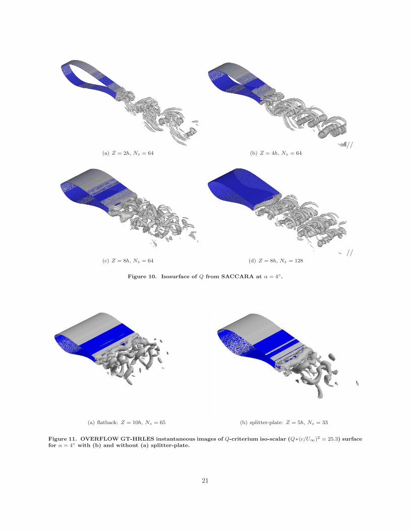
The frequency of vortex-shedding was seen to correlate quite closely to the peak noise frequency in theprevious section. Further, significant correlation was observed in the sectional lift coefficients (Cl) in the 3-Dsimulations with the level of correlation dependent upon the span-wise resolution. To investigate this, we havevisualized the coherent 3-D flow structures in the airfoil wakes. Following Dubief and Delcayre,58 one mayidentify coherent structures through iso-surfaces of the Q-criterion. The iso-surfaces of Q× (c/U∞)2 = 25.3for the six 3-D simulations at 4 are shown in Figs. 10 and 11 for SACCARA SADES and OVERFLOWGT-HRLES results, respectively.

In the SACCARA simulations with a spanwise resolution (δz) finer than h/16 (0.1c/16), there are well-defined 2-D rollers with 3-D braids between these. This is most clearly visible in Figs. 10(b) and (d) wherethe spanwise extent is 4h (0.4c) or more. This same flow structure is present in the 2h simulation, but it ismore difficult to observe. While there are more resolved 3-D turbulent flow structures in these higher resolu-tion cases, the spanwise correlation of Cl reported in Table 15 is higher due to the presence of the coherent2-D rollers. Lower δz resolutions predict more unorganized wake flow patterns with poorly defined rollers.However, based on the shedding frequency and aeroacoustic sound levels, there is evidence of bluff-bodyvortex shedding in these cases. From this, it appears that the less resolved spanwise instability wavelengthsare leading to incoherent vortex shedding for the coarser resolution cases. Note that the more incoherent

19

0 0.4 0.8 1.2 1.6 2Reduced frequency (St = f h/U)

0

20

40

60

80

100

Sou

nd P

ress

ure

Leve

l (dB

)

Flatback (OF GT-HRLES)Splitter-plate (OF GT-HRLES)

Figure 9. Sound pressure level (SPL) for a 3-D 10 flatback and splitter-plate airfoil simulations using OVER-FLOW with GT–HRLES.

shedding associated with coarser spanwise resolution actually improves agreement with the measured ex-perimental mean drag coefficient. Also note that aerodynamic and aeroacoustic quantities for the 8h/128case pictured in Fig. 10 have not been reported because it has not yet reached a statistical steady state.It is not clear which vortex-shedding mode more accurately reflects what is observed in experiment: themore two-dimensional roller with braid structure predicted by the finer resolution cases or the less coherentthree-dimensional shedding. Further work is needed to determine if more three-dimensional structure canbe induced in the fine-grid cases by, for example, altering the initial conditions.

Comparing the wake features predicted by SACCARA and OVERFLOW show similar wake structures(see Figs. 11(a) and 10(b)). However, the flow structures dissipate more rapidly with OVERFLOW. Whilethe wake resolutions in the near-field are similar, the SACCARA mesh maintains the resolution furtherdownstream which may explain the reduced dissipation. An exact matching of conditions is required to ruleout numerical algorithm effects.

The distinction between the wake flow with and without the splitter-plate is difficult to discern in theOVERFLOW GT–HRLES simulations. Both predict a highly incoherent shedding pattern following thedescription above. Simulations at twice the spanwise resolution (not shown) are currently underway whichfollow the trend of increased coherence with the observation of 2-D rollers and braids. Statistical analysis ofthese simulations will be reported in the near future.

VII. Conclusion

Computations of the flatback version of the DU97-W-300 airfoil in two and three dimensions usingtraditional RANS turbulence models and hybrid RANS/LES turbulence simulation techniques within CFDcodes have been accomplished. Several conclusions on the efficacy and future promise on the aerodynamicand aeroacoustic prediction capability of these advanced turbulence methods can be drawn:

• Time-averaged lift prediction is insensitive to grid, domain size, and simulation mode (steady RANSvs. unsteady hybrid RANS/LES), and both RANS and hybrid RANS/LES methods typically predict

20

(a) Z = 2h, Nz = 64 (b) Z = 4h, Nz = 64

//

(c) Z = 8h, Nz = 64 (d) Z = 8h, Nz = 128

//

Figure 10. Isosurface of Q from SACCARA at α = 4.

(a) flatback: Z = 10h, Nz = 65 (b) splitter-plate: Z = 5h, Nz = 33

Figure 11. OVERFLOW GT-HRLES instantaneous images of Q-criterium iso-scalar (Q∗(c/U∞)2 = 25.3) surfacefor α = 4 with (b) and without (a) splitter-plate.

21

lift coefficients within experimental bounds for the two angles of attack examined (4 and 10). Asthe angles of attack are relatively mild with primarily attached flow, significant differences in the liftcoefficients predicted by RANS and hybrid RANS/LES are not expected, as noted in prior applications.

• Time-averaged drag is consistently lower and more accurate for RANS than for unsteady hybridRANS/LES in two dimensions, as expected. The unstructured drag simulations using both RANSand hybrid RANS/LES are the exception to this, as both provide mean drag coefficients that are veryclose or within experimental bounds. In three-dimensions, while the unsteady simulations predict alower drag than two-dimensional simulations, further study to provide guidance on grid independencyis needed. The improved correlation of the drag on grids with larger spanwise computational domainsappears to result from wake structures that have more three-dimensional features.

• For the finest grid SACCARA simulations, The RMS lift fluctuation is highly correlated along thespan (C′

Lrms ≈ C′lrms) for all unsteady simulations. For α = 4 degrees, C′

Lrms is highest for the two-dimensional simulations and lowest for the simulation on the 0.8c (largest computational extent) grid.It decreases for α = 10 degrees.

• Strouhal number of the vortex shedding is insensitive to grid resolution, domain size, and angle ofattack, but appears to be 10to15% lower than experiment.

• The RMS drag fluctuation is not as highly correlated (C′Drms < C′

drms) as the lift fluctuation (C′Lrms ≈

C′lrms) for the SACCARA three-dimensional simulations.

• Aeroacoustic predictions using both approximate theory and integrated surface pressures from thesimulations agree well with one another. For the α = 10 case, simulation predictions are within 4 dBof experimental values, with the level of agreement dependent on the grid resolution, domain size, andcode used. OVERFLOW predicted a decrease in SPL due to the splitter plate of 5 dB at α = 10.

Acknowledgments

This work was supported in part by the National Science Foundation, Project 0731034, ”AdvancingWind Turbine Analysis and Design for Sustainable Energy”. The authors would like to thank NSF and theNSF Program Officer, Dr. Trung Van Nguyen, for their support in this endeavor. Additional funding wasprovided by Sandia National Laboratories, Wind Energy Technology Department, under contract #793065.Sandia is a multiprogram laboratory operated by Sandia Corporation, a Lockheed Martin Company forthe United States Department of Energy’s National Nuclear Security Administration under contract DE-AC04-94AL85000. Computational support for this research was supported in part by the National ScienceFoundation through TeraGrid59 (grant # TG-MSS080017N) and Sandia National Laboratories. TeraGridresources were provided by NCSA and SDSC.

The authors would like to thank James Erwin at Pennsylvania State University for his aid in obtainingacoustic data from the computations, as well as the FUN3D Development Team for their aid in the FUN3Dsimulations.

References

1Hubbard, H. and Shepherd, K., “Wind turbine acoustics,” TP 20320-77, NASA, December 1990.2Hubbard, H. and Shepherd, K., “Aeroacoustics of large wind turbines,” Acoustical Society of America Journal , Vol. 89,

June 1991, pp. 2495–2508.3Migliore, P. and Oerlemans, S., “Wind tunnel aeroacoustic tests of six airfoils for use on small wing turbines,” Journal

of Solar Energy Engineering , Vol. 126, November 2004, pp. 974–985.4Standish, K. and van Dam, C., “Aerodynamic analysis of blunt trailing edge airfoils,” Journal of Solar Energy Engi-

neerging , Vol. 125, Novemeber 2003, pp. 479–487.5Paquette, J. A. and Veers, P., “Increased Strength in Wind Turbine Blades through Innovative Structural Design,”

Proceedings of the European Wind Energy Conference, 2007.

22

6Berg, D. E. and Zayas, J. R., “Aerodynamic and aeroacoustic properties of flatback airfoils,” AIAA Paper 2008–1455 ,2008.

7Baker, J., Mayda, E., and van Dam, C., “Computational and Experimental Analysis of Thick Flatback Wind TurbineAirfoils,” AIAA Paper 2006–0193 , 2006.

8Brooks, T. F., Pope, D. S., and Marcolini, M. A., “Airfoil self-noise and prediction,” NASA RP-1218 , 1989.9Sorensen, N. N., Michelsen, J. A., and Schreck, S., “Navier-Stokes Predictions of the NREL Phase VI rotor in the NASA

Ames 80ft x 120 ft wind tunnel,” Wind Energy , Vol. 5, 2002, pp. 151–169.10Duque, E. P. N., Burklund, M. D., and Johnson, W., “Navier-Stokes and Comprehensive Analysis Performance Predictions

of the NREL Phase VI Experiment,” Solar Energy Engineering , Vol. 125, 2003, pp. 457–467.11Strawn, R. C., Caradonna, F., and Duque, E., “30 Years of rotorcraft computational fluid dynamics research and devel-

opment,” Journal of the American Helicopter Society , Vol. 51, No. 1, 2006.12Spalart, P. R., Jou, W.-H., Strelets, M., and Allmaras, S. R., “Comments on the Feasibility of LES for Wings and on a

Hybrid RANS/LES Approach,” Advances in DNS/LES , edited by C. Liu and Z. Liu, Greyden Press, 1997, pp. 1–20.13Kim, W.-W. and Menon, S., “A new dynamic one-equation subgrid-scale model for large-eddy simulations,” AIAA Paper

95-0356 , 1995.14Erlebacher, G., Hussaini, M. Y., Speziale, C. G., and Zang, T. A., “Toward the Large-Eddy Simulation of Compressible

Turbulent Flows,” Journal of Fluid Mechanics, Vol. 238, 1992, pp. 155–185.15Ghosal, S., “On the large eddy simulation of turbulent flows in complex geometries,” Center for Turbulence Research:

Annual Research Briefs, 1993, pp. 11–128.16Strelets, M., “Detached eddy simulation of massively separated flows,” AIAA Paper 2001-0879 , 2001.17Smagorinsky, J., “General circulation experiments with the primitive equations,” Monthly Weather Review , Vol. 91,

No. 3, 1993.18Barone, M. and Berg, D., “Aerodynamic and Aeroacoustic Properties of a Flatback Airfoil: An Update,” AIAA Paper

2009-0271, 2009 ASME Wind Energy Symposium, 2009.19Baurle, R. A., Tam, C. J., Edwards, J. R., and Hassan, H., “Hybrid Simulation Approach for Cavity Flows: Blending,

Algorithm, and Boundary Treatment Issues,” AIAA Journal , Vol. 41, No. 8, 2003, pp. 1463–1480.20Sanchez-Rocha, M., Wall-Models for Large Eddy Simulation Based on a Generic Additive- Filter Formulation, Ph.D.

thesis, Georgia Inst. of Technology, 2008.21Wilcox, D., Turbulence Modeling for CFD , CDW Industries, La Canada, CA, 2nd ed., 1998.22Sanchez-Rocha, M., Kirtas, M., and Menon, S., “Zonal hybrid RANS–LES method for static and oscillating airfoils and

wings,” AIAA Paper 2006-1256 , 2006.23Kok, J., Dol, H., Oskam, B., and van der Ven, H., “Extra large eddy simulations of massively separated flows,” AIAA

Paper 2004-0264 , 2004.24Stone, C., Tebo, S. M., and Duque, E., “Computational fluid dynamics of flatback airfoils for wing turbine applications,”

AIAA Paper 2006-0194 , 2006.25Lynch, C. E. and Smith, M. J., “Hybrid RANS–LES Turbulence Models on Unstructured Grids,” AIAA Paper 2008–3854 ,

2008.26Menter, F., “Two-equation eddy-viscosity turbulence models for engineering applications,” AIAA Journal , Vol. 32, No. 8,

1994, pp. 598–605.27Smith, M. J., Wong, T.-C., Potsdam, M., Baeder, J., and Phanse, S., “Evaluation of CFD to Determine Two-Dimensional

Airfoil Characteristics for Rotorcraft Applications,” Journal of the American Helicopter Society , Vol. 51, No. 1, 2006.28Shelton, A. B., Braman, K., Smith, M. J., and Menon, S., “Improved Turbulence Modeling for Rotorcraft,” Proceedings

of the 62nd American Helicopter Society Annual Forum, Phoenix, AZ, May 9-11,2006 , 2006.29Renaud, T., D. M. O’Brien, J., Smith, M. J., and Potsdam, M., “Evaluation of Isolated Fuselage and Rotor-Fuselage

Interaction Using CFD,” Journal of the American Helicopter Society , Vol. 53, No. 1, 2008, pp. 3–17.30Menon, S. and Kim, W.-W., “A New Dynamic One-Equation Subgrid Model for Large-Eddy Simulations,” AIAA Paper

1995–0352 , 1995.31Speziale, C. G., “Turbulence Modeling for Time Dependent RANS and VLES: A review,” AIAA Journal , Vol. 36, No. 2,

1998, pp. 173–184.32Timmer, W. and van Rooij, R., “Summary of the Delft University wind turbine dedicated airfoils,” J. Solar Energy

Engineering , Vol. 125, 2003, pp. 488–496.33Berg, D. and Barone, M., “Aerodynamic and Aeroacoustic Properties of a Flatback Airfoil,” 2008 AWEA Windpower

Conference, 2008.34Wong, C. C., Blottner, F. G., Payne, J. L., and Soetrisno, M., “Implementation of a parallel algorithm for thermo-chemical

nonequilibrium flow solutions,” AIAA Paper 95-0152, January 1995.35Yee, H. C., “Implicit and Symmetric shock capturing schemes,” NASA-TM-89464, May 1987.36Sjogreen, B. and Yee, H., “Multiresolution wavelet based adaptive numerical dissipation control for high order methods,”

J. Scientific Computing , Vol. 20, No. 2, 2004, pp. 211–255.37Spalart, P. R., Jou, W.-H., Strelets, M., and Allmaras, S. R., “Comments on the feasibility of LES for wings, and on

a hybrid RANS/LES approach,” Advances in DNS/LES, 1st AFOSR International Conference on DNS/LES, Greyden Press,1997.

23

38Girimaji, S. S., “Partially-Averaged Navier-Stokes model for turbulence: A Reynolds-Averaged Navier-Stokes to DirectNumerical Simulation bridging method,” J. Appl. Mech., Vol. 73, 2006, pp. 413–421.

39Buning, P., Parks, S., Chan, W., and Renze, K., “Application of the Chimera Overlapped Grid Scheme to Simulation ofSpace Shuttle Ascent Flows,” Proceedings of the Fourth International Symposium on Computational Fluid Dynamics, Vol. 1,1991, pp. 132–137.

40Ahmad, J. and Duque, E., “Helicopter rotor blade computation in unsteady flows using moving overset grids,” Journalof Aircraft , Vol. 33, No. 1, 1996, pp. 54–60.

41Meakin, R., “Moving grid overset grid methods for complete aircraft tiltrotor simulations,” AIAA Paper 93-3350 , 1993.42Lim, J. and Strawn, R., “Prediction of HART II rotot BVI loading and wake system using CFD/CSD loose coupling,”

AIAA Paper 2007–1281 , 2007.43Duque, E., van Dam, C., and Hughes, S., “Navier-Stokes simulations of the NREL combined experiment Phase II rotor,”

AIAA Paper 99-0037 , 1999.44Meakin, R., “Unsteady simulation of the viscous flow about a V-22 rotor and wing in hover,” AIAA Paper 95-3463 ,

1995.45Potsdam, M. A., Venkateswaran, S., and Pandya, S., “Unsteady low Mach preconditionging with application to rotorcraft

flows,” AIAA Paper 2007-4473 , 2007.46Bonhaus, D., An Upwind Multigrid Method For Solving Viscous Flows On Unstructured Triangular Meshes, Masters

thesis, George Washington University, 1993.47Anderson, W., Rausch, R., and Bonhaus, D., “Implicit/Multigrid Algorithms for Incompressible Turbulent Flows on

Unstructured Grids,” Journal of Computational Physics, Vol. 128, No. 2, 1996, pp. 391–408.48OBrien, D. M. and Smith, M. J., “Analysis of Rotor-Fuselage Interactions Using Various Rotor Models,” AIAA 43rd

Aerospace Sciences Meeting, Reno, NV , 2005.49Biedron, R., Vatsa, V., and Atkins, H., “Simulation of Unsteady Flows Using an Unstructured Navier-Stokes Solver on

Moving and Stationary Grids,” Proceedings of the 23rd AIAA Applied Aerodynamics Conference, Toronto, Canada, 2005.50Chorin, A., “A Numerical Method for Solving Incompressible Viscous Flow Problems,” Journal of Computational Physics,

Vol. 2, No. 1, 1967, pp. 12–26.51Roe, P., “Approximate Riemann Solvers, Parameter Vectors, and Difference Schemes,” Journal of Computational Physics,

Vol. 43, No. 10, 1981, pp. 357–371.52Kravchenko, A. G. and Moin, P., “Numerical Studies of Flow over a Circular Cylinder at ReD = 3900,” Physics of Fluids,

Vol. 12, No. 2, 2000, pp. 403–417.53Blevins, R., Flow-Induced Vibration, Krieger Publishing Company, Malabar, FL, 2nd ed., 2001.54Norberg, C., “Fluctuating Lift on a circular cylinder: review and new measurements,” J. Fluids and Structures, Vol. 17,

2003, pp. 57–96.55Hennes, C., Lopes, L., Shirey, J., and Erwin, J., “PSU-WOPWOP 3.3.2 User’s Guide,” Tech. rep., The Pennsylvania

State University, 2008.56Hennes, C. and Brentner, K., “The effect of blade flexibility on rotorcraft acoustics,” Proceedings of the 31st European

Rotorcraft Forum, 2005.57Brentner, K. and Farassat, F., “Analytical comparison of the acoustic analogy and kirchoff formulation for moving

surfaces,” AIAA Journal , Vol. 36, No. 8, 1998, pp. 1379–1386.58Dubief, Y. and Delcayre, F., “On coherenent-vortex identification in turbulence,” Journal of Turbulence, Vol. 1, No. 11,

2000.59Catlett, C., “TeraGrid: Analysis of Organization, System Architecture, and Middleware Enabling New Types of Appli-

cations,” HPC and Grids in Action, Ed. Lucio Grandinetti, IOS Press ’Advances in Parallel Computing’ series, Amsterdam,2007 , 2007.

24