a computer-aided study of the graded lie algebra of a ... · journal of pure and applied algebra 91...
TRANSCRIPT

Journal of Pure and Applied Algebra 91 (1994) 2555315
North-Holland 255
A computer-aided study of the graded Lie algebra of a local commutative noetherian ring *
Jan-Erik Roos Department of Mathematics. University of Stockholm, S-106 91 Stockholm, Sweden
Dedicated to Steve Halperin on his 50th birthday
Abstract
Roos, J.-E., A computer-aided study of the graded Lie algebra of a local commutative noetherian
ring, Journal of Pure and Applied Algebra 91 (1994) 2555315.
We initiate a systematic study of the homotopy Lie algebra gR of a local commutative noetherian
ring R. Particular emphasis is put on the sub Lie algebra qR, generated by elements of degree 1. The
computer is used in an essential way to detect new phenomena and new structure results, which are
then proved by hand calculations. In Appendix B (by Clas Liifwall) it is proved that in many cases
(including many examples encountered in this paper) gR is a nice semi-direct product of qR by means
of a free graded Lie algebra.
1. Introduction
Let (R, m) be a local commutative noetherian ring with maximal ideal m and residue
field k = R/m. Let ExtR*(k, k) be the corresponding Ext-groups. It is known that under
Yoneda product, the graded algebra
Ext;(k, k)
is even a Hopf algebra [ 131 (cf. also [28] and [29] for other references) and in fact it is
the enveloping algebra of a graded Lie algebra gR:
ExtR*(k, k) 7 U(gR).
This Lie algebra gR (called the homotopy Lie algebra of (R, m) and sometimes also
denoted n*(R)) says a lot about the singularity of (R, m) but its structure in general is
almost completely unknown. Let me just recall that:
Correspondence to: J.-E. Roos, Department of Mathematics, University of Stockholm, S-106 91 Stock- holm, Sweden. Email: [email protected].
*Appendix B written by Clas Liifwall.
0022-4049/94/$07.00 0 1994 Elsevier Science B.V. All rights reserved SSDI 0022-4049(93)EOO64-B

256 J.-E. Roes
(1) The following conditions are equivalent:
(a) gX = 0 for some i > 0,
(b) g6 = 0 for i 2 3,
(c) (R, m) is a local complete intersection.
Furthermore, (R, m) is regular if and only if gk = 0 for i 2 2. (2) If we define the radical rad(g,) of the Lie algebra gR as the sum of the solvable
ideals s of gR (an ideal s is solvable if the sequence s 2 [s, s] z [[s, s], [s, s]] z . .
reaches 0 after a finite number of steps, where e,g. [s, s] is the ideal of linear
combinations of [x, y], where x ES and YES), then rad(g,) is finite-dimensional and
the sum of the dimensions of its even degree parts is I dim,(m/m2) - depth(R).
(3) If dimk(m/m “) - depth(R) _< 3 then gR is a Lie algebra extension of a nilpotent
Lie algebra (situated in degrees 1 and 2) by means of a free Lie algebra.
Suitable references to the results (l))(3) can be found for (1) (results by Tate,
Assmus, and Halperin) in [13] and [14], for (2) in [ll] and for (3) in 141. There are
similar results (and problems) for the “equivalent” problem concerning the Lie algebra
of homotopy groups (under Whitehead product) of a finite (say), simply connected
CW-complex (the analogy is most striking for rational homotopy groups).
But apart from the previous results, very little is known in concrete situations:
Many of the current rings studied in algebra are either invariant rings of reductive
algebraic groups or determinantal rings defined by the annihilation of determinants of
certain matrices of indeterminates, or rings defined by some general construction, e.g.
the ring of the singularity of commuting n x IZ matrices of indeterminates. The
preceding rings are Cohen-Macaulay rings (in the last example at least for n = 3), but
this assertion should be only considered as the first step towards a more precise
theory. If (R, m) is a Cohen-Macaulay ring, and if you divide out by an R-sequence
you come down to an artinian local ring (R, fi), which has almost never been studied
in detail.
In a situation like this when little is known and the hand calculations of explicit
examples are hard, it is very natural to use the computer. This will be done in this
paper, where we will also prove theorems, inspired by the results obtained by our
computations.
Here is a summary of the present paper: In Section 2 we prove some elementary
results about the relations between a local Cohen-Macaulay ring and the associated
artinian ring and as a warm-up we study the homotopy Lie algebra in a special case.
This leads to Section 3, where we introduce a class of rings (R, m) (satisfying the
condition d3-this class contains the class of those rings for which m3 = 0), for which
the study of the homotopy Lie algebra gR is reduced in a nice way to the study of the
smaller Lie algebra yap of the primitive elements of the subalgebra of Ext,*(k, k),
generated by Exti(k, k) (we also introduce “higher” variants of J&: JZ~ and _Ys which
can be most easily understood by means of a complex C,(R) which we introduce for
any local ring (R, m)).
Our study is continued in Section 4 where we prove some new general results about
the relations between the Lie algebras ylR and gR. In particular we prove that for rings
The graded Lie algebra of a local commutative noetherian ring 251
(R, m) satisfying m3 = 0 the sub Lie algebra, gc (consisting of the elements of degree
> t in gR) is a free Lie algebra if and only if qzf 1s a free Lie algebra. In [2], Avramov
defines R to be generalized Golod of level I t if gzf . IS free and he proves that for such
R all finitely generated R-modules have a rational Poincare-Betti series of a nice form
(earlier Avramov and Felix proved similar results for CW-complexes [3]). In Section
5 comes the main exotic examples of the structure of gR (and vR) found among rings of
the form
k[X,, X2, X3, X,]/(quadratic forms in the Xi’s)
and their quotients. We are able to describe the Lie algebra gR in all these cases and in
particular we obtain the first examples where yap is not nilpotent and gz” is free but
gz3 is not free.
In passing we also answer (negatively) some questions that have been posed by
Irena Peeva and David Eisenbud.
In Section 6 we describe very briefly some examples in embedding dimension 5 and
higher, in particular an irrationality and convergence example (“the Opera Cellar
Case”), which we like.
In Section 7 we present some (according to our opinion) reasonable conjectures in
this area.
In Appendix A I present some technical details about how I used the computer to
find my results. I hope this will be useful for mathematicians.
Finally, Appendix B (written by Clas Liifwall) contains all those useful results that
he obtained when the tried to answer some of my questions, that were inspired by my
computations. I wish to express my sincere thanks to him for having written down
these results, and for having been willing to discuss these problems with me.
Besides Clas Liifwall, I also wish to thank many other mathematicians and
computer scientists for stimulating discussions and useful help, in particular: Luchezar
Avramov, Jiirgen Backelin (whose program BERGMAN was extremely useful), Rick-
ard Bogvad, Torsten Ekedahl, Ralf Friiberg, Hubert Grassmann, Bernd Herzog,
Joachim Hollman, Freyja Hreinsdottir, Calle Jacobsson, A. Kustin, . . and finally
Dave Bayer and Mike Stillman, whose beautiful program MACAULAY [9] started
these investigations.
A general assumption: In order to avoid extra complications we assume throughout
that the characteristic of the residue field k = R/m is diferent from two.
2. Connections between a Cohen-Macaulay ring and the associated artinian ring
It follows from [13] and [21] that if R is a local ring, t is a non zero-divisor in R, and
R = R/(t) then the ring map R -+ l? is either a large map, i.e. the induced map
Ext;(k, k) + Ext;r(k, k)

258 J.-E. Roos
is a monomorphism, or R + R is a Golod map, i.e. the induced map
Ext;(k, k) + Ext,*(k, k)
is an epimorphism with a Hopf algebra kernel which is a free algebra (in this special
case on one generator of degree 2). The first case occurs if t is in m but outside m2 and
the second case occurs if t is in m2. In particular the Lie algebra gE is either a sub Lie
algebra of gR of codimension 1 (they differ only in degree 1) or gR is a quotient algebra
of gR with kernel of dimension 1 (they differ only in degree 2). Iterating this observa-
tion we arrive at the following proposition:
Proposition 2.1. Let R be a Cohen-Macaulay ring, (r 1, . . , rt) the ideal generated by
an R-sequence, R the corresponding quotient ring and R -+ R the corresponding ring map
inducing a map of Ext-algebras,
Ext;(k, k) + Ext,*(k, k),
and thereby a map of the corresponding Lie algebras,
This map is an isomorphism in degrees > 2 and ifthe R-sequence is linearly independent
modulo m2 then the map is even a monomorphism which is an isomorphism in degrees
>l. 0
Thus for the study of the essential part of the Lie algebra gR, it is for Cohen-
Macaulay rings sufficient to study artinian rings. This reduction is very useful when
one is using a computer. In Appendix A, I will describe how this is done in practice.
We now turn to a more detailed study of the Lie algebra gi of the artinian ring l?.
I claim that in many cases it is for many purposes sufficient to study the Lie
subalgebra no of gR generated by the set of elements of degree 1. Let me just give an
example to illustrate this:
Example. Let U and V be two 3 x 3 matrices of indeterminates Xi, . . ., Xr8:
The condition that these matrices commute, U V = VU, leads to 9 quadratic equa-
tions in the XI’s, which generate an ideal I in the ring k[X,, . . ., X,s]. It was Mike
Artin who asked (more generally for n x n-matrices) whether the corresponding

The graded Lie algebra of a local commutative noetherian ring 259
quotient ring R = k [X 1, . . ., X,,]/Z was a CohenMacaulay ring. This was proved
by Bayer and Stillman using the computer program MACAULAY [9] for the case
y1 = 3 (cf. Example A.3) but the general case is open (cf. the note at the end of the
paper). We will now show how one can dig deeper and get information about the Lie
algebras gR and gR for n = 3:
Indeed the ring R in question is Cohen-Macaulay of dimension 12, hence one
can reach an artinian ring R by dividing out a linear R-sequence of 12 elements
(cf. Example A.3). One then reaches an artinian ring R with Hilbert series
1 + 6t + 13t2 + lot3 + t4.
Let rl~ be the sub Lie algebra of gc generated (as a graded Lie algebra) by the
elements of degree 1. It follows from Theorems B.2 and B.9 that the inclusion map
v],- + gi can be split by a Lie algebra map n and that we have an exact sequence of
graded Lie algebras
wheref is a free graded Lie algebra.
It follows that the two Lie algebras gE and VR are closely related. The important
thing now is that it is possible to use the computer algebra program MACAULAY, to
prove that VR is a nilpotent Lie algebra. Indeed, writing for simplicity f instead of VR,
we have that q is generated as a Lie algebra by its elements of degree 1. Thus to prove
that f is nilpotent it is sufficient to prove that one of the yl”s is zero, for then it follows
that the qj’s for j > i are zero too. Let us now use the program MACUALAY to
calculate parts of the first (bi)graded Betti numbers of R (i.e. for each i the dimensions
of the graded vector space dimJExti(k, k))). Introduce l? to MACUALAY-more
details in Appendix A-, issue the command:
nres R t 4
and then break the computations after a while and issue the new command:
betti t
We get as an answer the scheme:
total: 1 6 23 73 ???
0: 1 6 23 70 183 (2.2)
1: --~ 3 ??
(The question marks means that the corresponding computations have not been
finished. The important thing is however that the calculation of the middle horizontal
row is finished and this is so since the calculations in the last row have been started,

260 J.-E. Roes
leading to at least one betti number, namely 3.) The numbers in the middle horizontal
row are the first coefficients in the Hilbert series
A(t) = f dim,(A’)t’, i=O
(2.3)
where A is the enveloping algebra of q. This series can be expressed as an infinite
product;
(2.4)
where for any vector space V’ over a field k, we write 1 VI = dim,(V). Then 1$1’s are
called the (sub)deviations of l? and the 1$1’s are called the deviations of l?. The
numbers 1 ij’l are uniquely determined by the series on the left-hand side of (2.3). More
precisely, the 1 ij’l’s in degree < v are uniquely determined by the series A(t) in degree
< v. Furthermore, a “four-line” MATHEMATICA program for calculating the I ij i I’s
from the series A(t) is given in Example A.6. Using this (but it can also be done by
hand calculations), we get that the dimensions of vi, q, q3 and q4 are 6, 8, 2 and 0.
From what we just have said above it follows that all the $‘s are 0 for i 2 4 so that
&qt) = (1 + t)V + t312 (1 - t2)s
and the Lie algebra q is nilpotent of index 3.
From what we have done so far we get the following theorem:
Theorem 2.2. Let R be the “universal” singularity of two commuting 3 x 3 matrices, and
gR the homotopy Lie algebra of R. The Lie algebra gR is free in degrees 2 4 but not free
in degrees 2 3.
Indeed, in degrees 2 2 the Lie algebras gR and gR above are isomorphic (Proposi-
tion 2.1). It follows from the exact sequence (1) and the fact that v], is nilpotent of index
3 that gR is isomorphic to the free Lie algebra fin degrees 2 4. If gE were free in
degrees 2 3 its sub Lie algebra SIR would be so too. But in degrees 2 3 we have just
seen that v], is isomorphic to the abelian Lie algebra on two generators in degree 3 and
this last Lie algebra is not free. 0
Remark. It is of course interesting to try to determine all the (bi)graded Betti numbers
of R (and R) in the example we have just studied. For this we need to make a much
more precise study of the conections between the Hopf algebras B = Ext,*(k, k) and
A = the subalgebra of B, generated by Ext ‘,(k, k) both for R and t?. This will be done
in the next two sections.

The graded Lie algebra of a local commutative noetherian ring 261
3. A natural generalization of rings having & = 0. Conditions MS, ZS and a useful
complex
The conditions As
Let (R, m) be a local commutative noetherian ring. Let k = R/m and let B be the
Yoneda Ext-algebra Ext,*(k, k) and A the subalgebra of B, generated by Exti(k, k).
Both Liifwall [23-251 and I [28], have made a thorough study of the relationship
between A and B in the case when m3 = 0. Of course, many rings that occur “in
nature” do not satisfy m 3 = 0 but it often occurs that their properties are “m3 = O”-
like. The aim of the present sdction is to give definitions and to prove precise results
about this. First note that if A4 is any R-module then the Yoneda product
Ext;(k, k) @ Ext;(M, k) + Ext;+” (M, k)
makes Ext,*(M, k) to a left Ext,*(k, k)-module.
In Section 1 of [28] I observed (cf. Theorem 1’ on p. 295) that if a is an ideal of an
arbitrary local ring (R, m) then we have an exact sequence of graded left
B = Ext,*(k, k)-modules:
_ O~s~‘S,-,s~lExtR*(R/ma,k)~ BOkExtk(R/a,k)
and
-r;Ext;(R/a,k)+S,+O (3.1)
_ Ohs-‘S,~s~‘ExtR*(R/ma,k)~BO,Ext~(R/u,k)
(3.2)
where for any graded B-module N, (s- ‘N)” = N”- ‘, N denotes the elements of N of
strictly positive degrees, Y is the Yoneda product and S, is defined as the cokernel of
Y in (3.1) Clearly we also have an exact sequence
where k has the “trivial” graded B-module structure. In [28], from the middle of p. 295
and onwards we assume m3 = 0 and we go on and use (3.1) and (3.2) for a = m and
a = m2 and prove the formula (22) of Theorem 3 of p. 298 (lot. cit.). More precise
homological relations between the algebras A and B are given on pp. 298-306 (lot.
cit.). (Note that (22) was first proved by Liifwall [25] in a different way in the
equicharacteristic case, cf. Remark 8 on p. 298 of [28] for more details). But it was
262 J.-E. Roes
quite clear that one could go further if m3 # 0 and we will do that now: First some
notations: If V is a graded vector space over a field k,
v= @vi it0
we define the Hilbert series V(z) of V as follows:
V(z) = c dim, Viz’. iZ0
Even if (R, m) is not graded, we define the Hilbert series HR(z) of R as the Hilbert series
of the graded associated ring. The Poincare-Betti series of R is the Hilbert series of
B = Extg(k, k) and it will be denoted by Ps(z). With these notations the following
result follows easily from (3.1) and (3.2):
Proposition 3.1. Let (R, m) be any local ring, PR(z) the Poincar&Betti series qf R and
HR(z) the Hilbert series of R. Then we have the following identity offormal power series,
PR(z)HR( - z) = 1 + (1 + z) 1 ( - z)~&++I(z)
k20
= (1 + 2) c ( - Z)kSm’(+*(Z),
k20 (3.4)
where .?,,,k+ 1 and S ,++I are dejined by the sequences (3.1) and (3.2).
Proof. Put a = mk for varying k in (3.1) and (3.2), observe that the alternating sums of
the Hilbert series in (3.1) and (3.2) are zero and combine the results. 0
Corollary 3.2. Let (R, m) be a local ring such that
(*) f,++2=0 fork>O.
Let A be the subalgebra of Extg(k, k) generated by ExtA(k, k). Then we have the
following formula relating the Poincarb-Betti series PR(z), the Hilbert series A(z) of
A and the Hilbert series HR(z) of R:
PR(z)-’ = (1 + l/z)/A(z) - HR( - z)/z. (3.5)
Proof. The formula (3.4) gives that
PR(z)Hix( - z) = 1 + (1 + z)%(z).

The graded Lie algebra qf a local commutative noetherian ring 263
Furthermore, Theorem 2 on p. 297 of [28] gives the following formula valid for any
local ring:
PR(Z) = A(z)Sm(z). (3.6)
Now replace S,(z) by 1 + g,,,(z) in (3.6) and eliminate f,Jz) from (3.4) and (3.6). This
gives formula (3.5). 0
Remark 3.3. If m3 = 0 then of course ( * ) is true and (3.5) is as we said well-known. In
[28] cases were given where m 3 # 0, m4 = 0 but nevertheless ( * ) was satisfied. In the
present paper we will give many more examples.
Definition. (i) We say that a local ring (R, m) satisfies the condition A3 if (R, m)
satisfies the condition (*) above.
(ii) More generally, we say that (R, m) satisfies the condition Jt?S (s fixed, s 2 2) if
(es) S,k+S-,=O fork20
Remark 3.4. If the maximal ideal m of a local ring (R, m) satisfies mk = 0 then
R satisfies the condition &k, but the converse is not necessarily true. Indeed, it is, for
example, clear that (R, m) is a “Koszul algebra” (also called a “Friiberg ring”) if and
only if R satisfies AZ [6,25,28]. Furthermore, it follows from the results of Levin [19,
201 (the ArtinRees lemma is used) that for any local commutative noetherian ring
(R, m) there is an integer no > 0 such that R satisfies Mk for all k > no. More details
are given below.
Remark 3.5. In the graded case, i.e. when R is a quotient of a polynomial ring
k[ X1, . ., X,] (where the generators Xi have degree 1) by an ideal generated by
homogeneous elements, it is clear that the vector spaces ExtL(k, k) have an extra
grading, so that we can introduce a Poincare&Betti series in two variables
P,(x, y) = 1 dim,Exti(k, k)jx’yj it0, j>i
(3.7)
It follows easily that if (R, m) satisfies JZ~ then we have then even more precise
two-variable version of (3.5)
PR(X> YF l = (1 + l/X)/WY) - ffR( - XY)lX, (3.8)
and of course this formula reduces to (3.5) if we put y = 1. The formula (3.8) is
extremely useful for testing with the computer program MACAULAY if a graded
(R, m) satisfies A3. Indeed, MACAULAY calculates a diagram of Betti numbers of

264 J.-E. Roos
a quotient of a polynomial ring k[Xl, . . ., X,] by a homogeneous ideal up to a
degree specified by the user which can look as follows if the homological degree
specified is 3:
total: 1 6 23 73
0: 1 6 23 70 (3.9)
1: -- ~ 3
The numbers in the middle horizontal row are the dimkExtk(k, k)’ = dim,(A’)
and the whole diagram (3.9) gives PR(x, y) up to the degree in x that is specified.
Furthermore, the Hilbert series of the local ring is also determined by
MACAULAY.
A useful complex. The conditions ZS
For any local commutative noetherian ring (R, m) we will now construct an
extremely useful complex from the exact sequences (3.1) and (3.2) (for varying a) above:
First consider the exact sequence (3.1) for a = m, then take sP1 of (3.2) for a = m2, se2
of (3.2) for a = m3, etc. We get a set of exact sequences:
O-kS-'s,+S -‘ExtR(R/m2, k) 3 B Ok ExtA(R/m, k)
5 Exti(R/m, k) + S, --f 0,
o+ sm2s m2 + sm2Extg(R/m3, k) 5 s-‘(B OkExtL(R/m2, k))
~s-‘Ext~(R/m2, k)+ sP1Sm2-+0,
_ o+s-3s,s+s- 3Extj$(R/m4, k) ysP 2(B Ok Extb(R/m3, k))
xss2EXtE(R/m3, k)+ sC2$,,,” --+ 0,
etc.
where Y, Y’, Y”, . . are Yoneda products and where the maps X, X’, X” are defined
by the diagram. It is now clear how to turn the right vertical column and
B = Ext,*(R/m, k) into a complex of left B-modules:
... +s -2(B Ok Exti(R/m3, k)) Esm’(B@kExti(R/m2, k))
%B@kExti(R/m, k)4 B.

The graded Lie algebra of a local commutative noetherian ring 265
This complex C,(R) is extremely useful for studying a local ring (R, m) and we will
now determine its homology explicitly. First we need some notations: Since gmn is the
image of the natural restriction map
Ext;I(R/m”, k) -+ Ext;(R/m”+‘, k)
it follows that the s,,, form an inductive system whose transition maps we will denote
by i,,,. In particular we have natural maps
We are now ready to calculate the homology of C,(R):
Theorem 3.5. Let (R, m) be a local commutative noetherian ring, and C,(R) tlze complex
of B = Extz(k, k)-modules introduced above.
(i) Using the previous notations the homology H, = H,(C,(R)) sits in the middle of
an exact sequence
+ s~(~-~)(~,,,~-~ n Ker(Exti(R/m”, k)+ Extff(R/m”+‘, k))+ 0 (3.10)
(this sequence is also valid for small n 2 0 if we interpret gmo as zero, write Ho, etc.).
(ii) The condition A?, is verified (i.e. S,j = Oforj 2 s - 1) ifand only ifHi = 0
for i 2 s.
(iii) Let gS be the condition that the complex C,(R) is spherical at s - 1, i.e. that
Hi(C*(R)) = Ofor i # 0, s - 1. Then YS and M, are equivalentfor s = 2 and s = 3 and
for s 2 4 we have that
=% * M, and smi i’,‘+ 1 , ,Y?,,,, + I are isomorphisms for i = 1, , s - 3.
Proof (i) follows by an easy diagram chasing. Let us prove (ii). First if S,j = 0 for
j 2 s - 1 it follows from (3.10) that H,(C,(R)) = 0 for n 2 s. The converse is slightly
more tricky: We need the Artin-Rees lemma, used as in [19, 201. Thus we assume
H,(C,(R)) = 0 for n L s and recall that Levin proved that for any local commutative
noetherian ring R there always exists a to such that the image of the map:
mi(R/m’, k) + Exti(R/m’+‘, k) is zero for t 2 to. Let us assume that to is chosen as
small as possible. If to < s, then in particular s,, = 0 for i 2 s - 1 (2 to) and the
converse assertion is proved. Thus we can assume to 2 s. But then H,,(C.J = 0, and
the formula (3.10) for n = to gives that gmrO- 1 = 0, which contradicts the fact that
to was chosen as small as possible.

266 J.-E. Roos
To prove (iii) we first note that we always have
fFm2 H,(C*(R)) = S-l ~ ( 1 il,2(Sm) .
Thus if A3 holds, i.e. $,,,L = 0 for i 2 2, then H,(C,(R)) = 0, proving the equivalence
of ~%!s and Zs. The conditions A3 and L& are the same and it is clear that if they hold,
then C,(R) is a minimal resolution of S,. Assume now that s 2 4. If M, is true then
(3.10) shows that H,(C,(R)) = 0 for 1 I i I s - 2 if and only if
Smj+l
ij,j+l(Smj)
=0 forj= l,...,s-2
and
$,,,-I n Ker(Exts(R/mj, k)+ Extz(R/mj+‘, k)) = 0
forj=2,...,s-2.
Inspection of the diagram
O”,O Ext,*(R/mj, k) - S,, - Ext,*(R/m’+ ‘, k)
I ‘Id+1
I mi(R/m’+‘, k) A S,j+l v
now gives the result and the Theorem 3.5 is completely proved. Cl
Remark 3.6. Inside the Hopf algebra B = Exti(k, k) we have the subalgebra A gener-
ated by Exti(k, k) and the previous construction of C,(R) can be done over this
smaller algebra A instead of B. We then get a smaller complex C,(R) of left A-modules,
and we have a natural isomorphism of complexes: B Oa C,(R)%C,(R). Since B is
a free right A-module it follows that we also have an isomorphism of homology
groups
and that for a fixed i H,(C,(R)) = 0 if and only if Hi(C*(R)) = 0. It follows that there
is a version Theorem 3.5’ of Theorem 3.5, where we work over A instead of B and that
Theorem 3.5’ and Theorem 3.5 are equivalent (we do not give details, just an
indication: m,*(R/mj, k) should be replaced by A.Exti(R/mj, k), etc.). The complex
C,(R) has been introduced in another way in Appendix B, when R is “2-homogene-
The graded Lie algebra of a local commutative noetherian ring 267
ous”. Indeed our complex C,(R) is the dual (over k) of the complex U (lot. tit), and
Liifwall denotes C,(R) by R* Ok A is Appendix B (and he uses an upper grading,
which is only a minor notational difference from our lower grading). In particular,
Theorem B.3 (combined with Lemma B.l) gives an alternative proof of the equiva-
lence:
&k 0 Hi(e*(R)) = 0, for i 2 k
Liifwall’s explicit calculations with R* Ok A in Appendix B will be extremely impor-
tant in Sections 5 and 6.
Remark 3.7. If a ring (R, m) satisfies _Pk for some fixed k 2 3, then Theorem 3S(iii),
combined with the formulae (3.4) and (3.6) gives a generalization of the formulae (3.5)
and (3.8). This generalization is not written down here, since Lofwall has proved it
(first) in Theorem B.4 in another way in the “2-homogeneous case”. The ring in
Case VIII in Section 5 satisfies JZ’~ but not Zj.
Remark 3.8. If
Ext; (R/m’, k) --f
is zero then R+ RJm’+’
Exti(R/m’+‘, k) (3.1 l)t
is a “strong Golod map” [20,21]. If t = 2 and if
(R, m) is graded in the sense described above then the following conditions are
equivalent:
(I) Extz(R/m’, k)+ mg(R/m3, k) is zero.
(II) R + R/m3 is a Golod map.
(III) R + R/m3 is a strong Golod map.
An example in the non-graded case where (II) is true but (I) is false is
R = kCx, yll(x2 + y3, XY).
For t 2 3, even in the graded case, it is not true that (3.1 lh is zero if R -+ R/m’+ ’ is
Golod, even if one supposes that the map (3.1 l)f_ 1 is zero. Indeed, using formulae
(3.1), (3.2) for a = m, m2, . . . and (3.6) it is, for example, easy to prove if (R, m) is graded
and (3.11), is zero then the following are equivalent:
(a) (3.11)3 is zero.
(b) l+z Z (1 + l/Z) ffR,m‘d - Z) ~ - ~ = PR(Z) PR/m4(Z) A(z) - z
and R + R/m4 is Golod. (3.12)

268 J.-E. Roes
(c) The two-variable version of(b):
1+x X (1 + l/X) HR,m4 - XY)
my)- hw(X,Y)= AbY) - x
and R -+ R/m4 is Golod. (3.13)
Of course there are versions for higher t and condition (c) and its higher variants are
very suitable for testing on a computer.
Remark 3.9. Let (R, m) be a local graded Gorenstein ring with m4 = 0. Let A be the
subalgebra generated by ExtA(k, k) in Ext,*(k, k). Then ~k’~ is verified, so that the
equations (3.5) and (3.8) are true. Indeed, if m3 # 0 then since the socle is l-dimen-
sional (R is Gorenstein), the socle must be equal to m3 and Avramov and Levin
proved [S] that R + R/m3 is a Golod map (if the embedding dimension of (R, m) is
> 1, which we can assume). Now apply the equivalence (I) o (II) above. If m3 = 0 the
result is even easier to prove.
Here is a variant of the preceding result: Assume that (R, m) is a local graded
Gorenstein ring with ms = 0 and that R -+ R/m3 is a Golod map. Then 4?, is still
verified. Indeed, we can assume m4 # 0. In this case R + R/m4 is still a Golod map.
Then ~,4’~ is still verified. Indeed, we can assume m4 # 0. In this case R -+ R/m4 is still
a Golod map but Levin and Avramov actually proved that stronger statement that
(3.1 1)3 is zero [S, 203. Since R + R/m3 is supposed to be Golod the map (3.1 1)2 is zero.
It is evident that the higher (3.11), for t > 3 are all zero. Thus, the condition M3 is
verified.
Remark 3.10. We have been unable to prove that the ring R of the commuting 3 x 3
matrices of Section 2 satisfies kC3. Since @is = 0 it is clear that A5 is satisfied, but it
follows from Theorem B.9, that also _4Z4 holds true. It remains to prove that for the
ring l? in question we have that the map
Ext&+ii2, k) + Ext;(l?/ti3, k)
is zero. If this is the case, then the formula (3.8) predicts that PR(x, y) is equal to
(x2yZ - xy + l)*
~"y"~8s'y'+4~~y'+28s~y~ -8x"J'b~56~5y5+8~4y5+70~4J~4-3~3y4-56s~~3+28~2J~2~8xy+1
which has the Taylor series expansion
1 + 6xy + 23x2y2 + (70~~ + 3y4)x3 + (183~~ + 34y5)x4

The graded Lie algebra of a local commutative noetherian ring 269
+ (428~~ + 217~~)~’ + (918~~ + 1022~~ + 9y8)x6
+ (1836~’ + 3943~~ + 150y9)x7 + (3465~’ + 13156~~ + 1351y”‘;s’
+ (6226~~ + 39220~” + 8702~~~ + 27~“)~~
+ (10725~” + 10674Oy” + 44811~” + 594~‘~)~‘~ + 0(x”)
leading to that prediction that MACAULAY should produce the following table of
graded Betti numbers for fi:
total 1 6 23 73 217 645 1949 5929 17972 54175 162870
0: 1 6 23 70 183 428 918 1836 3465 6226
1: _ 3 34 217 1022 3943 13156 39220
2: _ _ _ 9 150 1351 8702
3: _ _ _ _ _ 27
10725
106740
44811
594
The second horizontal row (in boldface) is of course already calculated completely
(cf. Section 2). The other numbers are predicted, and if MACAULAY would give
something different anywhere in the table, then M3 would not hold for l?. But using
about 2.3 MB internal memory, MACAULAY calculates the first 5 columns rather
easily (the commands are:
nres l? t 4
betti t
and the first 5 columns come out as they should after 201 minutes and 49 seconds on
a Sparcstation 1 with 64 MB of internal memory). If you try the commands
nres l? t 5
betti t
you do get that the first 6 columns come out as they should, but this time you have to
use a SPARCSERVER 690MP and you have to wait about 96 hours and use 30 MB
of internal memory.
Remark 3.11. In all the remaining explicit cases studied in this paper with the
exception of Case VIII in Section 5, the condition A3 is verified, and in most cases the
proof of the validity of d3 is a consequence of results proved in Appendix B.
4. A theorem about sub Lie algebras of gR and VfR
Recall (cf. the Introduction) that a local ring (R, m) is said to be generalized Golod of
level < t if the sub Lie algebra gzf of the homotopy Lie algebra gR, consisting of the
elements of degree > t is a free Lie algebra.

270 J.-E. Roes
Theorem 4.1. Let (R, m) be a local commutative noetherian ring with maximal ideal
m and residue field k = R/m. Assume that m 3 = 0 The following assertions are equiva- .
lent:
(i) (R, m) is generalized Golod of level I t.
(ii) The sub Lie algebra of Extg(k, k) generated by ExtA(k, k) is free in degrees > t.
Proof. Since a sub Hopf algebra of a free Hopf algebra is itself free, we clearly have
(i) * (ii).
The converse is slightly more tricky: Put B = Exti(k, k), A = the subalgebra of
B generated by ExtA(k, k). Then we have the following two exact sequences of left
B-modules (formulae (17) and (18) of p. 295 of [28] and the same sequences as (3.1) and
(3.2), for a = m)
_ O+ splSm-+ s-1(B@kExt~(R/m2, k))+ B@,ExtA(k, k)
5 B + S, -+ 0, (4.1)
O-+S,,,+S,+k+O, (4.2)
where for any graded B-module M, (s -‘M)” = M”- ‘, Y is the Yoneda product and
S, is defined as the cokernel of Yin (4.1) [S, is the part of S, that is in strictly positive
degrees].
Let us now write A and B as enveloping algebras of graded Lie algebras:
A = U(n) and B = U(g)
We want to prove that if v] ” is a free Lie algebra, then so is g”. But if S is a sub Hopf
algebra of a Hopf algebra H then H is a free S-module [27], so that in particular
Torf”“‘(k, k) = Tor, “(q’(k @ o(s”) u(g)> k) (4.3)
and similarly
Torf’““‘(k, k) = Tor, ““‘(k 0 “(,,>I) u(n), k) (4.4)
We know that the left-hand side of (4.4) is zero for n > 1 and we want to prove the
same result for (4.3). Let M be the right B = U(g)-module k @ UCq>~j U(g). Now tensor
the exact sequence (4.2) to the left with the right B-module M. We obtain an exact
sequence
. . . + Tor:(M, S,) + Torf(M, k) + Torf_ ,(M, S,) + . . . (4.5)

The graded Lie algebra of a local commutative noetherian ring 271
But (4.1) implies (note that the three middle B-modules in (4.1) are B-free) that for
n>l
Torf_l(M, F’S,,,) = Tor:+2(M, S,) (4.6)
and since clearly S, = B Oak the right group of (4.6) and the left group of (4.5) are
isomorphic to Tort+z(M, k) and Tort(A4, k), respectively. Thus we have an exact
sequence for n 2 2
. . -+ Torff(A4, k) + Tor:(M, k) + Tort+2(M, s(k)) + . (4.7)
where s is the inverse of s -I. But it is almost clear (see below) that as a right A-module,
M is a direct sum of copies of N = k @ uc,>~,U(q) and this last module N has the
property that
Tort(N, k) = Tory’““‘(k, k) = 0, for n > 1
Thus using (4.7), Theorem 4.1 is proved, modulo the “almost clear assertion”
which follows from the fact that we have an isomorphism of right U(g)-
modules,
where the right U(g)-module structure on the right is defined by the ring map
U(g) --f U(g/g”). Similarly
and
is a sub Lie algebra of
S/S” = g10g20 ‘.. Og’
so that U(g/g”) is a free U(q/q”)-module. 0
Remark 4.2. Clearly, under the hypotheses rn3 = 0 many other homological proper-
ties of A and B are also equivalent e.g. the properties that U(g”) and U(q”) have
homological dimension v, etc.

272 J.-E. Roes
Remark 4.3. In general (no assumptions on R) it is of course true that (i) *(ii) in
Theorem 4.1. The converse is much more difficult. If we weaken the condition m 3 = 0
to A3, i.e. if we suppose that the natural restriction maps
%f,*(R/m’, k) -+ Exts(R/m’+‘, k)
are zero for t 2 2, the method of proof in Theorem 4.1 only gives that g’f has global
dimension I 2. But if we also make the stronger assumption that ye is nilpotent of
index t, i.e. that ;rl” = 0 then g” is free.
This last assertion follows even if we suppose that instead of d3, the condition
_!Zk is satisfied for some k 2 2. This follows from Theorem B.2 combined with
Theorem B.3 (even more general results can be deduced). More examples will be given
in Sections 5 and 6, and for reasonable conjectures we refer the reader to Section 7.
5. C. Jordan and the computer
The aim of this section and the next is to describe how we got all the strange
examples in embedding dimension 4 and 5. We are fairly sure that we now have an
almost complete picture of the homotopy Lie algebras, Poincare-Betti series, etc., of
at least quotients of polynomial rings in four and five variables with respect to ideals
generated by quadratic forms, but at the moment we have no complete structure
theorem. We have therefore preferred to describe here how we found our examples
and to choose 8 typical examples, that we describe in detail (more details about how
the computer was used are given in Appendix A). In Section 6 we treat the case of
higher embedding dimensions and finally in Section 7 we present (according to our
intuition) reasonable conjectures about structure theorems.
In a series of papers, of which the last but one was [ 151, Jordan classified explicitly
all pairs of quadratic forms (under the equivalence of simultaneous linear transforma-
tion of the variables) in 2, 3, 4, . ., variables. A very good historical background of
this type of problem and an overview of all of Jordan’s results is given by J. Dieudonne
on pages vii-xiv of the third volume of Jordan’s collected papers [16] and the paper
by Jordan just cited is the first half of paper 119 in Dieudonne’s list of Jordan’s
publications. In particular there are 22 isomorphy classes of pairs of quadratic forms
in four variables of which there are 2 resp. 6 classes depending only on 2, resp.
3 variables. Of the 14 remaining classes (that really depend on 4 variables) only one
class has a parameter in it. More details are given in Section 10 of [15].
We now want to go further and understand the homological behaviour of quotients
of polynomial rings in four variables by means of 3 linearly independent quadratic
forms (and then four, five, etc.). The idea is very simple: There are 10 linearly
independent quadratic forms in 4 variables. We start with one of the 22 preceding
cases of 2 quadratic forms and we add a third one as a linear combination of
8 monomials which are not dependent of the 2 given quadratic forms. We have chosen

The graded Lie algebra OJ a local commutatiw noethrrian ring 273
to study the case in which the coefficients in the linear combination are 0 or 1. Then we
get 2’ = 256 different cases. It is very easy to generate these 256 cases from inside the
computer algebra program MACAULAY (more details are given in Appendix A) and
then we calculate by means of MACAULAY for each ring
R = U-x, Y, z, ull(fi,fi,fs)
where thefi’s are quadratic forms, the following:
(1) The Koszul homology of R.
(2) The standard basis of the ideal (fi ,f2, f3) and corresponding Hilbert series.
(3) The resolution of the residue field k = R/m of the ring R up to a certain degree.
Since this resolution is infinite we have to stop somewhere, but 6 or 7 betti numbers
seem to be sufficient to predict the general behaviour.
Then we apply MAPLE to get a suggestion of a corresponding rational function
(details in Appendix A) and finally we prove this result at the same time as we get
information about the corresponding Lie algebras, using some new ideas (cf. e.g.
“Indications of proofs” in Case I below), the theory of Sections l-4 and Appendix B.
In all we have to check 22 x 256 - 22 = 5610 rings of which clearly some can be
easily transformed into each other, but this transformation is not worth the effort,
since all this can be made automatic and calculated rather quickly (at least if we do not
ask for more than 6 or 7 betti numbers).
Here is the result of the calculations which we present as an observation:
Observation 5.1. Out of the 5610 rings mentioned above,
where fi, f2, f3 are quadratic forms in (x, y, z, u), the overwhelming number of rings fall
into case A, almost 600 into case C, about 200 into case B and the rest into D, E, F of
Table 1, where E and F are the most exotic (18 and 6 cases respectively).
The case E is the only case which does not come from a 3-variable situation. All other
cases can be explained by the results of Backelin and Friiberg [S] for the case of three
variables. In all cases the ring is either a Golod ring (cases C, D, F) or a complete
intersection (case A) or is the image of a Golod map from a complete intersection
(cases B, E). It follows that the homotopy Lie algebra is in all cases free in degrees 2 3.
Furthermore, the condition A3 of Section 3 is valid in all cases.
When we now pass to the case of four quadratic relations the situation changes
dramatically, and we will find cases where the homotopy Lie algebra is free only in
degrees 2 4 and where the Lie algebra of the subalgebra generated by Extk(k, k) is
free in degrees 2 4 but not nilpotent. These examples seem to be the first of their kind.
The general idea is still very simple: We start with some (preferably exotic) cases of
3 quadratic relations in four variables and we then add in a similar way as above

214 J.-E. Roos
Table I
Case Example Hilbert
of idea1 series H(t)
Poincart-
Betti P(t)
Double PoincarkBetti series P(x, y).
and irs first 4 or 5 terms,
i.e. P(x, y) =
by. Y2, z2) 1 + 2t- t3
(1 - tp
(XY,Y2, xz) 1 + 2t
(1 ~ ty
(X2,Y2,XZ + yu) 1 +2t-22tj+t4
(1 - t)2
by, Y 2T YZ) I + t - 2tZ + t3
(1 - t)3
1+t
(1 - t)’
(1 + t)*
1 - 2t + t3 - t4
(1 + t)*
1 -2t + t3
(1 + rs
1 - 2t
(1 + t)2
1 - 2t - t4
(1 + t)’
I - r - 2t2 - r3
P(yx) = 1 + 4yx + 9y2x2 + 16y3x3
+ 25y4x4.
(l + xY)2
1 - 2xy + 2X3Y3 - x3y4 - x4y4
= 1 +4yx+9y*xz
+ (16~’ + y4)x3 + ‘.
P(yx) = 1 + 4yx + 91,2x2 + 17413x3
+ 3oy4x4 ‘.
P(yx) = 1 + 4yx + 9y2xz + 18y3x3
+ 36~~~“.
(l + xY)2
1 - 2xy + 2x3y3 - 2x3y4 - x4y4
= 1+4yx+9yzxz
+ (16~~ + 2y4)x3 +
P(yx) = 1 + 4yx + 9yzxz + 19y3x3
+ 41y4x4. ‘.
a fourth quadratic form which we choose in 2’ = 128 possible ways. It is good that in
each instance we only have 128 cases, because the calculations of the betti numbers of
the quotient ring now become considerably harder. In some cases we need up to 12 or
14 or maybe even 16 betti numbers to be able to make a prediction of the Poin-
car&Betti series and this is not possible with MACAULAY unless you have (at least
in the last case) up to 1 GB ( = 1024 MB) of internal memory, an extremely fast
computer and lots of time. In those cases we had to prove first that the condition
_&TX holds (using Appendix B if necessary) so that it is sufficient to calculate the Hilbert
series of the non-commutative graded algebra A (cf. Section 3) and for this we use the
extremely useful and fast program BERGMAN (written by Jiirgen Backelin at the
Department of Mathematics of the Stockholm University). More details are given in
Appendix A. We then take a set of 4 quadratic forms (preferably chosen in an exotic
way) as relations and add a fifth form chosen in 26 = 64 ways, etc. Instead of
presenting our systematic studies here we choose to present the 8 most exotic cases for
quadratic forms in four variables with complete details and comments:

The graded Lie algebra of a local commutative noetherian ring 275
Case I
We take the ring with four quadratic relations:
R = k[x, y, z, ul/(x’ + xy, y2, xu, xz + yu)
Summary of results
(a) The Hilbert series of the subalgebra A generated by Exti(k, k) is equal to
(1 + z)” (1 - z + 22) Nz) = (1 - z)2 (1 - z - z2 _ z4 _ z5)'
(b) The Hilbert series of the ring R is
HR(t) = (1 + 2t - t2 - 2t3 + t4)/(1 - ty
= 1 + 4t + 6t2 + 6t3 + 7t4 + St5 +. .
(c) The ring R satisfies the condition A3 (cf. Section 3) so that the Poincare-Betti
series in 2 variables x and y of R is given by the formula
PR(X, Y)F' = (1 + llX)l~(XY) - ff( - XY)lX,
which in our case gives
PR(X, Y) = (1 + x3y3)(1 + xy)
1 - 3xy + 2x2y2 + x3y3 - 2x4y4 + x5y5 + x6y6 - x6y’ - x’y’
In particular, for the graded betti numbers of R we have Tor:,(k, k) = 0 for p # q
and p < 6 and Tort,,(k, k # 0 only for q = 7 and 6 and these two vector spaces are 1,
resp. 167-dimensional. This gives a negative answer to a question of Peeva and
Eisenbud who asked whether
Torfj(k, k) = 0 for i # j and i < dim,(m/m2)
implies that
TorFj(k, k) = 0 for all i # j.
(d) The subalgebra A = U(q) generated by ExtA(k, k) in Exti(k, k) has according
to the recipe of Liifwall [25] the presentation
k<T,, T2, T3r T4)
(T: - CT,, &I> CT,, T31 - CG, T41, CT,, &I, Tj', CT,, 7'41, Lf)

276 J.-E. Roos
where k( T,, T,, T3, T,) is the free associative k-algebra in variables Tl, T,, TX, T, of
degree I and where [T, q] = 7; q + TjTi is the graded commutator. Let l? be the
ring k[x, y, z, u]/(xz + yu, xu + y2). This ring is a local complete intersectiona nd it is
also a so called Froberg ring, so that in particular Extff(k, k) is equal to
Now the natural ring map R”+ R which induces a map of the corresponding Ext-
algebras, Extg(k, k) + Ext$(k, k), also induces a map on the subalgebras generated by
Ext ’ which induces a map of Lie algebras YI -+ y” which sits in an exact sequence of Lie
algebras,
o-tK+rf--+ij+o. (5.1)
One further proves that K in (5.1) is equal to the semi-direct product of a I-
dimensional abelian Lie algebra a in degree 3 and a free Lie algebrafgenerated by
finite-dimensional graded k-vector space
where the dimensions of Vi are 2,1,1,2,1 for i = 2,. . . ,6 and where the operations of
a can be explicitly described (cf. below). In particular, we have an exact sequence of Lie
algebras,
O-kf+IC+a+O. (5.2)
Since 6 is zero in degrees > 2 (R is a complete intersection) the sequence (5.1) shows
that K"; v'~. More generally K" G q" for all t 2 2. Now since a’ 3 = 0 the exact
sequence (5.2) implies that we have an isomorphismf”G q” for all t 2 3 and since every sub Lie algebra of a free Lie algebra is free we obtain that q’3 is a free Lie
algebra.
According to the theory of Sections 3 and 4 we obtain that l? = RJm3 has an
Ext-algebra Ext$(k, k) = U(g) where g --> 3 is a free Lie algebra which is not nilpotent (in
particular not zero). We use here that v] = q [25]. This ring R seems to be the first of its
kind that has been found. For R itself, and Extz(k, k) = U(g) we can for the moment
only prove that g’3 has global dimension I 2.
Remark. In this case it is too hard to use MACAULAY to make a prediction about
the betti numbers of this ring. Instead we use the program BERGMAN by Jorgen
Backelin to get a useful prediction about ,4(z). After that we must of course prove
everything:

The graded Lie algebra of a local commutatioe noetherian ring 277
Indications of proofs
Here is a sketch of how one proves by direct calculations that the subalgebra
A generated by Exti(k, k) is as asserted in Case I: In the paper by Cohen, Moore, and
Neisendorfer [lo], the authors study on p. 132 an exact sequence of “homology Hopf
algebras” over a ring, which we here take to be a field k:
k-+A’+A+A”+k. (5.3)
Since A is a free A’-module we have a natural isomorphism Tor$‘(k, k) + Tor:(A”, k)
which gives in particular a left action of the algebra A” on Tor<‘(k, k) = I(A’)/(I(A’)‘,
i.e. the space of indecomposable generators for the algebra A’. On the other hand the
Lie bracket [ ,] : A 0 A --t A induces a left A”-operation on I(A’)/I(A’)2. In Lemma
3.12 of [lo] the authors prove that these two left A”-module structures coincide. In
our special case the Hochschild-Serre spectral sequence for the extension of Lie
algebras (5.3) shows that the set of generators for the Hopf algebra U(K) is generated
as a fi-module by two elements in degree 2. Clearly one can choose as these generators
t1 = Tf ( = [T,, T,]) and c2 = T$ - [T,, T4]. Combining this with the fact men-
tioned above one sees that one obtains generators for U(rc) in degree 3 by letting the
generators T,, T,, T,, T, of U(n) operate by the adjoint map on the ti’s. Since K lies
inside q, we can use all the relations in n when we calculate, as well as the Jacobi
identity which for elements a, b, c of degrees Ial, 1 bl, ICI looks like
( - I)‘~‘.‘~’ [a, [b, c]] + ( - 1)“““’ [b, [c, a]] + ( - 1)“’ lb’ Cc, [a, bll = 0
(5.4)
We obtain
and
CT,>i”zl = ~2, C7’23521 = ~2 -PI, CT3,521 = 0, C7’4r521 = ~1,
where ,u~ and p2 are defined by these formulae, i.e. pl = [T,, T:] and p2 = [T,, T:].
Let us show quickly how for example the formula [T2, c2] = p2 - pi is obtained:
CT2,<21 = C7’2, T: - CT,, TJI = 0 - CT2,CTl, Tall
= CT,, CT4> T211 + CT43 CT,, T,ll
= CT,,CT,> 7,311 + CT,> T:l = - CTJ, T:l + CT,, T:l

278 J.-E. Roes
where we have used that [r,, r:] = 0, the Jacobi identity
the facts that [r,, T2] = [r,, T3] and [T,, T,] = r: in q and finally the fact that
The other formulae are proved in a similar way. It follows that we have found at
most two new generators in degree 3: ,LL, and pLz. We now continue and let the Tts operate on the p;s. We obtain
where u is defined by these formulae above. Thus we have found at most one new
generator of degree 4, namely u. We now continue and let the Tts operate on u. This
gives
Thus if we now continue with the operations of the Ti:s we see (using (5.4)) that no
new possible indecomposable generators are found. We therefore now try to find
possible relations between tl, c2, p, , pLz and U. We clearly have (the second equality of
(5.5))
C~,,C~I,P~II = C~,>CT,>ull = 0 (5.6)
where the last equality comes from the Jacobi identity
CT~,CTZ>UII - CT,, lu> Tdl + Cu> CT3, Tzll = 0,
the fact that [T3, u] = 0 (5.5) and that [T,, T,] = 0 in 9.
But if we apply the Jacobi identity to the left-hand side of (5.6) we obtain
so that cl: = 0 (we have always assumed that the characteristic of k is # 2). Further-
more, if we apply the Tls to the formula ,u: = 0 we get only one interesting relation,

The graded Lie algebra of a local commutative noetherian ring 279
namely [pi, u] = 0. Summing up, we obtain the following candidate for a presentation
of the enveloping algebra U(K) of the Lie algebra K by generators and relations:
where 2,) z2, fil, ii2 and ii are variables of degree 2,2,3,3 and 4. But
and clearly
k<b,,fQ (P:, El 3 4)
= k[C] @ E(F,).
Using the formulae for the Hilbert series of a tensor product and for
[18, p. 1081 it follows that the Hilbert series of U(K)candidate is equal to
1 + 23 1 _2z2_z3 - z4 - zz5 - 26
(5.7)
a coproduct
It is also easy to see that a coproduct as (5.7) above can hav: no nontrivial elements of
positive degree in its center.
Note however that we have so far only proved that U(K) is a quotient of U(rC)candidale
above. To prove that the natural onto map
is an isomorphism we do as follows: Let the generators of the free algebra
k(T1, T2, T3, T4) operate on the generators of the free algebra k(fl;, f2, ,il, /&, G)
by the formulae, inspired by our calculations above,
T,.5; = 0, T,.r2 = fi2,
T2.5; = 0, T,& = ji2 - j&,
T,& = jil, T& = 0,
T4& = b2, T4.F2 = fin>
T1.h = u”, T,.b2 = Ckt21, T~.fi = C4;,iiJ>
T,.,ii, = 0, T,.ji, = ii, T2.E = &i&l,
T3.j& = 0, T3.ji2 = 0, T3.ii = 0,
T4./ll = 0, T4./12 = 0, T4.G = - C~2>ihl>

280 J.-E. Roes
and extend these as graded derivations on the augmentation ideal of
k(r,, f2,~,,ji,,fi) so that, for example,
and more generally
Ti.(flj) = (Tf.f)tj + ( - l)“f”(Ti.g)
when,f”and Q are homogeneous elements of positive degrees of k ( Fl, 12, ii1, ji2, 9) and
If1 is the degree off: It is easy to see that the ideal (fi:, [bi, fi]) of k(i;, , r2, ,L,, ,&, ji) is
invariant under our operations, so that in fact T1, T,, T,, T4 operates on
U(K) candidate. Thus the whole algebra k( T1, T,, T3, T,) operates on U(K),,“didate. By
calculating further one sees that the elements Tf - [T,, T2], T:, [T,, T3],
[T,, T,] - [T2, T4], [T3, T,], Ti of k(T1, T2, T3, T4) give the zero operations on
U(K) candidate SO that U(q) operates on U(K)candidate. Furthermore it is easily seen that
the elements 5, = Tf = [IT,, T,], t2 = T: - [T,, T,], etc. in U(K) (lying inside U(q))
operate on U(K)candidate as the commutator of [i, etc. By induction one sees that higher
Lie elements in 51, . . . , u operate on U(K)candidate as the commutator of the corres-
ponding Lie element in t,, . . . , IT. Thus if a Lie element in the generators of
U(K) candidate is mapped to zero by ?r then it must lie in the center of U(K),,“didate. But We
have just seen that this center is zero. Thus TC is an isomorphism. Thus K is built up as
asserted and
(1 + z)4 1 + z3 A(z) = (1 _ z2)2 1 _ zz2 _ z3 _ z4 _ zz5 _ z6
(1 + z)’ l-z+z2 =(11 -z-z~_z4_z5’
Remark. It follows also from what we have proved that U(K) is the semi-tensor
product T(V,) 0 E(pL,) [31], where E(pl) is the exterior algebra on one generator pi
(of degree 3), T(V,) is the tensor algebra on the graded vector space
where Vz is generated by e2 = [I and f2 = t2, V3 is generated by f3 = p2, V4 is
generated by e4 = U, V5 is generated by e5 = [pi, tl] and f5 = [/A~, t2] and V.5 is

The graded Lie algebra qf a local commutatioe noetherian ring 281
generated by e6 = [pi, ,uz] and where the operations of pl on T( V,) are given by its
values on the generators:
pt.e2 = e5, pl.,fZ =.f5, pl.f3 = e6, pl.e4 = 0,
pl.e5 IO, pl.j5 = 0, pl.e6 = 0.
Case II
We take the ring with five quadratic relations:
R=k[x,y,z,~]/(~~+xy,y~,~~,~~+yu,zu+~~).
Summary of results
(a) The Hilbert series of the subalgebra A generated by Exti(k, k) is equal to
(1 + z)(l - z + z”) A(z) = (1 - z)2(l - 22 - z”)’
(b) The Hilbert series of the ring R is
HR(t) = (1 + 3t + t2 - 2t3)/(1 - t)
= 1 + 4t + 5t2 + 3t3 + 3t4 + 3t5 + ..’
(c) The ring R satisfies the condition A3 (cf. Appendix B) so
car&Betti series in 2 variables x and y of R is given by the formula
that the Poin-
p,(x,y)-’ = (1 + w4l4xy) - ff( - XY)lX,
which in our case gives
PI&Y) = (1 + xy)(l - xy + x2yZ)
1 - 4xy + 5x2yz - 2x3y3 - x4y4 + 2x5y5 - x5y6 - x6y6’
In particular, for the graded betti numbers of R we have Tori,,(k, k) = 0 for p # q
and p < 5 and Torf,,(k, k) # 0 only for q = 6 and 5 and these two vector spaces are 1,
resp. 137-dimensional. This gives also a negative answer to questions of Peeva and
Eisenbud.
(d) The subalgebra A = U(q) generated by Extk(k, k) in ExtB(k, k) is built up in
a similar way (the proofs are similar) as in Case I. Thus R/m3 is still another example
where the homotopy Lie algebra is free but not nilpotent (in particular not 0) in
degrees > 3. For the homotopy Lie algebra of R we only know that its part of

282 J.-E. Roos
degree >3 has global dimension I 2. In our case it is also possible to prove that the
natural ring map (R, is the ring of Case I)
RI-+ R,J(zu + u’) = R
(R is the ring of Case II) is a Golod map.
Case III
We take the ring with five quadratic relations:
R = k[x, y, z, u]/(x” + xy, y2, xu, xz + yu, 2’).
Summary of results
(a) The Hilbert series of the subalgebra A generated by Exti(k, k) is equal to
(1 + z)(l - z + z2) A(z) = (1 _ z)3(1 - z - z2 - z4 - z5)’
(b) The Hilbert series of the ring R is
HR(t) = (1 + 3t + t2 - 3t3)/(1 - t)
=1+4t+5t2+2t3+2t4+2t5+2t6+ “..
(c) The ring R satisfies the condition .&Z3 (cf. Appendix B) so that the Poin-
care-Betti series in 2 variables x and y of R is given by the formula
PR (x, Y) 1 + x3y3
= 1 - 4xy + 5x2y2 - x3y3 - x3y4 - 3x4y4 + 3x5y5 - 2x6y7 - 2x7y7 + x7y8 + x8 y8 .
In particular, for the graded betti numbers of R we have Tor&(k, k) = 0 for p # 4 and
p < 3 and Torf,,(k, k) # 0 only for q = 4 and 3 and these two vector spaces are 1, resp.
26-dimensional.
(d) The subalgebra A = U(q) generated by Extk(k, k) in ExtR(k, k) is built up in
a similar way as in Case I. Thus R/m3 is still another example where the homotopy Lie
algebra is free but not nilpotent (in particular not 0) in degrees > 3. For the
homotopy Lie algebra of R we only know that its part of degree > 3 has global
dimension I 2.
Case IV
We take the ring with six quadratic relations:
R = k[x,y,z,u]/(x2 + xy,y2,xu,xz + yu,z2,zu + u’).

The graded Lie algebra of a local commutative noetherian ring 283
Summary of results
(a) The Hilbert series of the subalgebra A generated by Exti(k, k) is equal to
(1 - 2 + z2)2
A(z) = (1 - z)3(1 - 32 + 322 - 323)’
(b) The Hilbert series of the ring R is
H,(t)=1+4t+4t2.
(c) The ring R satisfies the condition A3 (evident) so that the Poincar&Betti series
in 2 variables x and y of R is given by the formula
PRb, Y) = (1 -xy+xZy2)2
1 - 6xy + 15x2y2 - 22x3y3 + 21x4y4 - 12x5y5 - x5y6 + 3x6y6
In particular, for the graded betti numbers of R we have Tor&(k, k) = 0 for p # q and
p < 5 and Torf,,(k, k) # 0 only for q = 6 and 5 and these two vector spaces are 1, resp.
192-dimensional. This gives also a negative answer to questions of Peeva and Eisen-
bud.
(d) In this case we do have m3 = 0 in the ring so it follows that the whole
Ext-algebra Extff(k, k) = U(g) is a semidirect product of A by a free algebra T(s- ’ M),
where M is the third syzygy of k over A, and A operates on this tensor algebra in the
natural way (see [24] and Appendix B). Furthermore, if A = U(q) then we can find an
explicit description of A and r] as follows: Consider the natural ring map
R”= k[x,y,z,u]/(xz + yu,xu + y',xu + z2)
1 R = k[x, y,z, #]/(x2 + xy, y2, z2, xu, xz + yu, zu + u”)
(5.8)
This map is certainly not a Golod map, but the first ring R is a complete intersection
which satisfies the Friiberg conditions. The map (5.8) induces a map of the subalgebras
generated by Ext’ inducing a surjection of Lie algebras 9 + Q so that we have an exact
sequence of Lie algebras (K is defined by the sequence)
o+ic+~+ij+o. (5.9)
Here fi only exists in degrees 1 and 2 (where it is 4 and 3 dimensional) and K sits in the
middle of an exact sequence which is a semi-direct product,
O-+z-+lc-+a-+O,

284 J.-E. Roos
where a is an abelian Lie algebra which is 2-dimensional and concentrated in degree 3.
Furthermore, z is the free Lie algebra on a graded vector space V, @ V, @
V4 @ I’, @ V6, where the dimensions of the vector spaces Vi are 3,2,3,6,3 and where
the operations of a on V, are easily given.
Thus in this case it is clear that y ‘3 is free and not nilpotent. Furthermore, since
m3 = 0 we have, by Theorem 4.1 that g’ 3 is free too.
Indications $proofs
The proof is similar to the proof in Case I.
Case V
We now give an example in 4 variables, where the subalgebra generated by Ext’ is
the enveloping algebra of a nilpotent graded Lie algebra y which is different from zero
only in degrees 1, 2 and 3:
We take the ring with four quadratic relations:
R = k[x, y,z, u],‘(x2 + xy, z2,xz + yu + zu, yz + xu).
Summary of results
(a) The Hilbert series of the subalgebra A generated by Extk(k, k) is equal to
1 + z3 A(z)= (1 _ z)4’
(b) The Hilbert series of the ring R is
H,z(t) = 1 + 3t + 2t2 - t3
l-t = 1 + 4t + 6t2 + 5t3 + 5t4 + ... .
(c) The ring R satisfies the condition A3 (cf. Appendix B) so that
PR (x, Y) = 1 + x3y3
1 - 4xy + 6x2y2 - 4x3y3 + x4y4 - x4y5’
In particular, for the graded betti numbers of R we have Tori,,(k, k) = 0 for p # q and
p < 4 and Torf,,(k, k) # 0 only for 4 = 5 and 4 and these two vector spaces are 1, resp.
39-dimensional.
(d) In this case the Lie algebra n which only exists in degrees 1, 2 and 3 has
dimension 4,4 and 1 in these degrees, and now it follows easily from the Theorem B.2
that the homotopy Lie algebra g of R is free in degrees > 3 but not free in degrees
> 2.
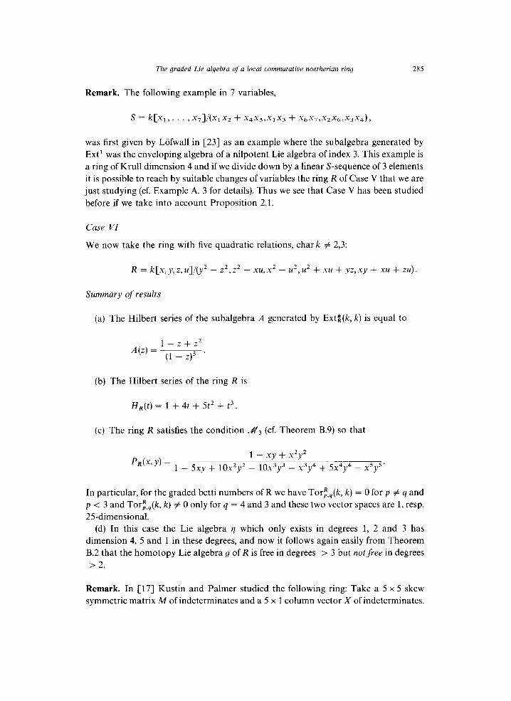
The graded Lie algebra of a local commutative noetherian ring 285
Remark. The following example in 7 variables,
s = k[Xl,. . . ) x7l/(x1x2 + x4x5>x1x3 + x6x,,x2x6,x3x4),
was first given by Lofwall in [23] as an example where the subalgebra generated by
Ext’ was the enveloping algebra of a nilpotent Lie algebra of index 3. This example is
a ring of Krull dimension 4 and if we divide down by a linear S-sequence of 3 elements
it is possible to reach by suitable changes of variables the ring R of Case V that we are
just studying (cf. Example A. 3 for details). Thus we see that Case V has been studied
before if we take into account Proposition 2.1.
Case VI
We now take the ring with five quadratic relations, char k # 2,3:
R = k[x, y,z, u]/(y2 - z2, z2 - xu,x2 - u2, uz + xu + yz,xy + xu + zu)
Summary of results
(a) The Hilbert series of the subalgebra A generated by ExtR(k, k) is equal to
l-z+z2 A(z) = (1 _ z)5 .
(b) The Hilbert series of the ring R is
HR(t) = 1 + 4t + 5t2 + t3.
(c) The ring R satisfies the condition M3 (cf. Theorem B.9) so that
PR(X, Y) = 1 - xy + x2y2
1 - 5xy + lOx2y2 - lOx3y3 - x3y4 + 5x4y4 - x5y5.
In particular, for the graded betti numbers of R we have Torf,,(k, k) = 0 for p # q and
p < 3 and Tori,,(k, k) # 0 only for q = 4 and 3 and these two vector spaces are 1, resp.
25-dimensional.
(d) In this case the Lie algebra n which only exists in degrees 1, 2 and 3 has
dimension 4, 5 and 1 in these degrees, and now it follows again easily from Theorem
B.2 that the homotopy Lie algebra g of R is free in degrees > 3 but not free in degrees
> 2.
Remark. In [17] Kustin and Palmer studied the following ring: Take a 5 x 5 skew
symmetric matrix M of indeterminates and a 5 x 1 column vector X of indeterminates.
286 J.-E. Roes
In total we have 10 + 5 indeterminates and we now consider the quotient S of the
polynomial ring in 15 variables by the ideal generated by the five quadratic relations
corresponding to the matrix equation M.X = 0. One can prove that S is a
Cohen-Macaulay ring of Krull dimension 11 and it can be proved that if we divide by
a suitable S-sequence then we come down to the ring R above. Now Proposition 2.1
shows again that Case VI is essentially the same example as that studied by Kustin
and Palmer [17], but the methods here give an alternative approach. In particular,
combining all this with Appendix B we obtain a new proof of their rationality results
for the Poincarl-Betti series.
Case VII
We now take the ring with six quadratic relations:
R = k[x, y,z, u]/(xu,zu, x2 + xy,z2, xz + yu, x2 + yz + d)
Summary of results
(a) The Hilbert series of the subalgebra A generated by Exti (k, k) is equal to
1 ,Qz) = (1 - z)2(1 - 22 - zz _ z3)’
(b) The Hilbert series of the ring R is
ffR(t) = 1 + 3t - 3t3
l-t =1+4t+4t2+t3+t4+ .“.
(c) The ring R satisfies the condition A3 (cf. Appendix B) so that
pR(x, Y) = 1 + xy
1 - 3xy + 3x3y3 - x5y6 - x6y6’
In particular, for the graded betti numbers of R we have Torf,,(k, k) = 0 for p # q
and p < 5 and Tort,,(k, k) # 0 for q = 6 and 5 and these two vector spaces are 1, resp.
225-dimensional. Thus it also gives a negative answer to the question of Peeva and
Eisenbud.
(d) In this case the Lie algebra q is an extension of a nilpotent Lie algebra Fj of
index 2 by a free Lie algebra on a graded vector space V2 @ V3 @ V4 0 V, where the
dimensions of the vector spaces Vi are 4, 5, 3, 1 and where the operations of Fj on V,
are easily given.
Remark. This case is probably not so exotic as the preceding six cases, since it might
be possible to reach this ring by a Golod map from a complete intersection.

The graded Lie algebra of a local commutative noetherian ring 287
Case VIII
We give one last example of embedding dimension 4 with four quadratic relations.
It is interesting for the reason that it is the only case we know of in embedding
dimension 4 with 4 quadratic relations where the condition A3 is not satisfied.
R = k[x, y, z, u]/(x2 + xy, xz + yu,z’, x2 + yz + u’).
Summary of results
(a) The Hilbert series of the subalgebra A generated by Exti(k, k) is equal to
1 A(z) = (1 _ z)4’
(b) The Hilbert series of the ring R is
HR(t) = 1 + 3t + 2t2 - 2t3 - 3t4
l-t =1+4t+6t2+4t3+t4+t5+ . . . .
(c) The ring R does not satisfy the condition J%‘~. Instead the Poincare-Betti series
in 2 variables x and y of R is given by the formula
p&G Y) = 1 + xy
(1 - xy)3( 1 - x2y2) - x3y5.
In particular, for the graded betti numbers of R we have Tor&(k, k) # 0 only if p I 4
and q - p is even.
(d) In this case the Lie algebra v] is nilpotent, and this ring satisfies the condition Z4
of Section 3. This gives the explicit formula for P,(x, y) above and also an explicit
presentation of U(gR) (cf. the last paragraph of Appendix B).
Historical note
In the first part of his thesis, Ralf Friiberg [12] proved that if R = k[Xl, . . . , X,1/1
where I is an ideal generated by (some) quadratic monomials in the Xi’s then the
Poincare-Betti series PR(z) and the Hilbert series HR(z) are related by the formula
PR(z) = l/H,( - z). (5.11)
In the thesis of Lofwall[25] several equivalent conditions are given (some of them due
to Backelin [6]) for the validity of the formula (5.11). The first counterexamples to the
validity of (5.11) when I is generated by quadratic forms were given independently by

288 J.-E. Roos
Christer Lech and Gunnar Sjodin [12]: Christer Lech noted that if I is generated by five
generic quadratic forms in 4 variables, then the Hilbert series of R must be 1 + 42 + 52’
but the Taylor series of l/(1 - 42 + 52’) = 1 + 42 + 1 1z2 + 24z3 + 41z4 + 442’
- 29z6 + 0(z7) has negative terms so a formula like (5.11) can never be valid. Gunnar
Sjiidin had essentially the same example, but it was very explicit:
R = k[x,y,z,u]/(x2 - y2,y2 - z2>Z2 - u2,XY>-= - YU).
One sees easily that A is the enveloping algebra of a Lie algebra which only exists in
degree 1(4-dimensional) and 2 (5dimensional). Later examples of these phenomena in
embedding dimension 3 were given by Friiberg and Backelin [S] - the so-called 3b
cases. However some of the examples we have given here are more sophisticated, since
they can not be reached by a Golod map from a complete intersection (indeed if R can
be reached in such a way then g,$’ is free).
6. Other examples
6.1. The embedding dimension 5 case
Here we will be much more concise. We hope indeed to come back to these cases in
a separate publication. We will only give three examples of rings that come up if we search
through many possible cases with the aid of the procedures, mentioned in Section 5.
R = k[x, y,z, u, v]/(y2, xy, yz + ZU, UU, u’)
This ring has a non-finitely generated Ext-algebra. I gave the first example of such
a ring in [28] but the example here has fewer relations and is in a sense simpler. The
Hilbert series is
- H(t) 1 + 2t - 2t2 3t3 + 4t4 - t5 =
(1 - t)3
= 1 + 5t + lot2 + 13t3 + 18t4 + 24t5 + ...
and the subalgebra A generated by Extk(k, k) has Hilbert series
(1 + z)3(1 - z) A(z) = (1 _ z _ z2)3
If we go through the constructions of Lemaire [18] where we replace the free algebra
in two variables of degree 1, by the algebra k( T1, T2)/( Tf) which has Hilbert series

The graded Lie algebra of a local commutative noetherian ring 289
(1 + z)/(l - z - z”) then we obtain a proof of the assertions here. I have also
calculated the To$(k, k) for i = 3,4,5,6, . . by means of BERGMAN and a
Govorov-Tor program of Backelin. These spaces turn out to be 13,1,1 and l-dimen-
sional etc. In [7], Backelin has also earlier been led to study this example.
R = k[x,y,z, u, v]/(x2,xy,xz + yu + zv,uv,v2)
Here the Hilbert series is
H(t) = 1 + 3t + t2 - 2t3 + t4
(1 - t)Z
= 1 + 5t + lot2 + 13t3 + 17t4 + 21t5 + 25t6 + .”
and
(1 + z)2 A(z) = (1 - z - ,2)2 n=l
fi 1 + z2n-i 1 - Z2” .
Furthermore the Lie algebra q is built up as an extension
O-+h -+vj-+e2xZ2-+0, (6.1)
where e2 is the Lie algebra of the ring k[x, y]/( x2, xy), E2 is the Lie algebra of the ring
k[u, v]/(v2, uv) and h is the free abelian Lie algebra which is l-dimensional in each
degree 2 1 and the extension (6.1) is defined by a 2-cocycle, just as it is in the case that
Lofwall and I studied in [26] (of course we were inspired by the results of Cl]). In the
case we treated in [26] the role of e2 x g2 is taken by f2 xT2 wheref2 is the free Lie
algebra which is the homotopy Lie algebra of k [x, y]/(x2, xy, y’) and similarly forf2 ).
The condition A3 is satisfied in Case 8 so that the Poincare-Betti series in two
variables of R is given by
P,(x,Y)-~ = (1 + ll4lWy) - H( - XY)/X
and the first part of the corresponding Taylor series looks like
1 + 5yx + 15y2x2 + 38y3x3 + 88y4x4 + (191~’ + y6)x5
+ (395~~ + lly7)x6 + (63~~ + 788y7)x7 + (1530~’ + 262y9)x8
+ (905~” + 2907~~)~~ + (5425~” + y” + 2771y”)~‘~
+ (17~‘~ + 7783~” + 9975~“)~” + O(X’~).

290 J.-E. Roes
Note 6.1. The preceding ring is also mentioned by Backelin in [7], but he did not
study the irrationality problem.
Note 6.2. Since A(z) is irrational, the preceding ring is of course “highly singular” and
as a matter of fact it can be obtained in the following way which emphasizes this:
Let (X, . . . X,) be 9 indeterminates and let Rg be the “universal ring” of the
singularity defined by annihilating the square of a 3 x 3 matrix, i.e. consider the matrix
of indeterminates
‘XI X2 X3
x = x, x5 x,
\X’ X8 X,
and take Rg = k[X1,. . . , X,]/(X’ = 0) where (X2 = 0) is the ideal generated by all
the 9 elements of the matrix X2 in k[X1,. . , X,]. Clearly this ring Rg is “very
singular”, and if we specialize Rg by putting some variables equal to zero we obtain
essentially the Case S? ring: Take, for example,
I 0 0 0
x=y x u
z 0 v
Then
and
i 0
x2 = xy + zu
ZV
\
1 0 0
x2 xu + uv
0 v2
k[x, y, z, u, v]/(X2 = 0) = k[x, y, z, u,u]/(x2, xy + zu, xu + uu,w 0’)
which is essentially the Case &?. Of course there are many more possibilities of
interesting rings, obtained by taking alternating, symmetric, etc. matrices of indeter-
minates, higher order matrices, etc.
Case % (The “Opera Cellar Case”)
R = k[x, y, z, u, v]/(x’, y2. z2, u2, u2, xz + yu + zv,yz + xv + zu, xu + yv)
This ring has Hilbert series 1 + 5t + 7t 2. More interesting is the subalgebra
A = U(q) generated by Exti(k, k) which has Hilbert series (char k # 2,7)
(1 -t @(l + z3)5(1 + z5)5(1 + z’)j(l + z9)5(1 + z11)3 A(z) = (1 _ z2)8(1 _ z4)4(1 _ z6)6(1 _ z8)3(1 _ z10)6(1 _ z12)3 .‘. . (6’2)

The graded Lie algebra of a local commutative noetherian ring 291
Note the periodicity here, which implies that the sequence dim,($) is bounded. It
follows that A(z) is an irrational function, which has a power series expansion, which
converges in the whole interior of the unit circle.
As far as I know this is the first known example of this phenomenon. Indeed,
according to Clas Liifwall, he and David Anick decided that if one of them found such
an example, then he would be invited by the other fellow to the “Opera Cellar
Restaurant” in Stockholm.
I have also calculated the Tor&(k, k) for i = 3,4,5,6 by means of BERGMAN and
a Govorov-Tor program of Backelin. These spaces turn out to be 0,1,6 and ?-
dimensional. Clearly there are variants of the preceding example, for example
R,,, = k[x, y, z, u, u]/(x2, y2, u2, u2, xz + yu + zv, yz + xu + zu,xu + yu)
which has Hilbert series
H,,,(t) = 1 + 4t + 3t2 - 5t3
l-t =1+5t+Xt2+3t3+3t4+3t5+ ..’
and whose A,,,(z) = A(z)(l - z2)(1 - z4)/(1 + z3)2 (thus it is almost the same as the
.4(z) of (6.2)). This ring satisfies condition J3. We hope to come back to this and
similar examples at a later occasion.
6.2. Higher embedding dimension cases
Recall that we have earlier defined what it means for (R, m) to be generalized Golod
of level I t. Let us say that (R, m) is generalized Golod of level exactly t if furthermore
(R, m) is not of level I t - 1 and let us say that (R, m) is of nilpotent type if the sub Lie
algebra generated by Exti(k, k) is nilpotent and A3 is verified. We have earlier seen
that in embedding dimension 4 there are (R, m) which are generalized Golod of level
exactly equal to 1, 2 and 3, both of nilpotent and non-nilpotent type. It would be nice
to see what happens in higher dimensions. Of course the reasoning in [29] shows that
the old example k[x, y, z, u, u]/(x2, y2, xy, xz + yu + zu, 12, uu, u2) is not generalized
Golod of any level and the same assertion holds for Case g above. But in a series of
papers Wisliceny [34,35] has studied the extremal cases of the possible degrees of
nilpotency of nilpotent Lie algebras, given by generators and relations. It is certainly
possible to develop his theory in the graded case. Instead of doing so we just mention
the following result which is very explicit, but not the best one:
Case 9
R = k[xl, . , ~,-~,u,u]/(m~,x,u + x2u,x2u + x3u,. . . ,
x,-3u + x,_2u,u2,u2)

292 J.-E. Roes
For each integer n 2 4, this is a local ring of embedding dimension n which is
generalized Golod (of nilpotent type) of level exactly
n - 2 if n is odd and n - 3 if n is even.
Here comes the proof of this: First note (for any R) that if the sub Lie algebra
v] generated by Extk(k, k) is such that @+i = 0 but @ # 0 then we have that qzS is free
(it is even zero), but for odd s q >’ is not free (its enveloping algebra has non-trivial
elements whose square is 0). Ifs is even, and dimkg” = 1 we have that ye >’ is free, but
that yZS-i is not free so that in both cases we have (if m3 = 0) according to Theorem
4.1 that (R, m) is generalized Golod (of nilpotent type) of level exactly s, ifs is odd, and
exactly s - 1, ifs is even. Now, in the case at hand it follows according to the recipe in
[25] that U(v) can be presented as the quotient of the free algebra
k(T1,. , Tnm2, U, V) with the ideal generated by the elements
CC, ul - CT,+l, V] for 1 I i 2 n - 3,
[Ti, Tk], 1 I i,k I n - 2,
CT,, VI, CT,-2, Ul and [U, VI.
But it is easily seen (proved by Lofwall who produced this example of Lie algebra
a long time ago) that the corresponding Lie algebra has in degrees 2 3 a vector space
basis all the elements of degree 2 3 among the
so that for n 2 4
Iv11 = n, I$ = n - 1,
Iqkl=n-k-l fork=3,...,n-2,
I#1 = 0, forj 2 n - 1.
This gives the result.
7. Conjectures and questions
It seems too early to put forward general conjectures about the structure of
B = U(gR) = ExtR(k, k) when (R,m) is a general ring of the form
kCXl>. > X,ll(f~, . . . J-t)

The graded Lie algebra of a local commutatioe noetherian ring 293
where thefi’s are quadratic forms in (Xi, . . , X,). At least the following seems to be
true:
(i) For n = 4 we have that A = U(v],), the subalgebra of Extg(k, k) generated by
Exti(k, k) sits inside B as in Appendix B, i.e. with the notations given there, the
homology of positive degrees of the complex R* @ A is concentrated only in one degree,
either in degree 2 (examples: Cases I-VII of Section 5) or in degree 3 (example: Case VIII
of Section 5). Furthermore ylR is free in degree 2 4 in all cases we have seen. If this were
true in general, it would follow that there are no irrational Poincare-Betti series PR(z)
for n = 4 and that the Lie algebra gR would sit in the middle of a split extension
wherefis a free Lie algebra. Will something of the preceding assertions survive in the
general embedding dimension 4 case (not necessarily quadratic relations)?
(ii) For n 2 5 it would be interesting to know where the non-zero homology of
R* @ A can be situated (we return to the case of quadratic relations). Are there
examples where this homology can be in two diflerent positive degrees? I guess that
there are no such examples for n = 5. But for higher n’s this can probably occur and it
would be interesting to know the exact limits (cf. the note at the end of the paper).
(iii) As we have mentioned earlier it would also be interesting to know the
homotopy Lie algebra of certain “universal” singularities. The determinantal singular-
ities with quadratic relations satisfy AZ but it would be nice to determine the
homological dimensions of the corresponding homotopy Lie algebra.
(iv) Another problem: Let R be a Cohen-Macaulay ring, and R = R/(an R-se-
quence). Are the conditions yk and/or &k true for R if and only if they are true for R?
(v) A technical problem: Let
R = kCX1,. . . > X,1 Vi>. . . 4)
where thefi are quadratic forms. Does there exist (at least for n I 5) a function N(n, t),
such that knowledge of the first N(n, t) betti numbers gives the rest of them?
(vi) The complexes C,(R) and C,(R) are objects in the derived category of lower
bounded complexes of finitely generated free B-, resp. A-modules having bounded
homology. More generally for each finitely generated R-module M we have a similar
complex. This should lead to interesting new invariants of local noetherian rings and
finitely generated modules over them.
Appendix A. Some technical details about how the computer was used
When I first started to use version 2.0 and later 2.17 of the program MACAULAY
in 1988 I was amazed by the possibilities of that program (resolutions of graded

294 J.-E. Roes
modules over graded polynomial rings, Hilbert series and standard bases of such
modules, etc.), but from my point of view the main drawback of version 2.17 was that
it was unable to handle resolutions over quotients of such polynomial rings. This
problem was solved by version 3.0 of Macaulay [9] that I got hold of in April 1989
(Macintosh and SUN3 version). But it was not until the SPARC(SUN4) version
became available later that year that I was able to make real progress with the
problems of this paper.
I will now give more details about how to do the computations hinted at in Section
5 since this might be useful for mathematicians who are unfamiliar with computers.
Thus what follows is a series of recipes and tricks, some of which might be useful in
other contexts. I do not claim to have presented the most elegant solutions, but they
work and are rather easy to understand. The methods are most easily described by
concrete examples.
Example A.l. This example shows a Macaulay scriptfile that is used to examine the
25 = 32 cases of rings where we have in k[x, y, z, u] a given ideal, defined by gener-
ators: (fi ,fz,f3,f4,f5) and add new linear combinations of 5 quadratic monomials.
(More details were given in Section 5). This scriptfile can be called from inside
Macaulay with the command line
< name of the scriptfile
On Unix systems you can also use the command
nohup macaulay < name_of_the_scriptfile > outputfile &
if you want to be able to logout without interrupting the calculations. You can then
login at a later occasion and examine the file outputfile.
Here comes the scriptfile (the commands inside the scriptfile are in boldface and the
comments are placed after the sign ;):
ring r
ideal j 5 y2 - 22 22 - xu x2 ~ u2 u2 + X” + yz xy + X” + Z” mat a
; We initialize a polynomial ring in 4 variables
; over a finite field of characteristic 31991 (the default), i.e. this line is empty. ; 4 variables
; The names of the 4 variables.
;The variables are given the weight 1 (the default), i.e. this line is empty.
; We have the reverse lexicographical order on the variables (the default). ; We now introduce the ideal generated by the f-i’s of Case VI of Section 5. ; We have 5 generators.
; We have now created the ideal j of Case VI in r.
; Now create a column matrix,

The graded Lie algebra of a local commutatioe noetherian ring 295
5 1
XY xz
YZ Y” ZU
mat m 2 1 0 1 mat K2 2 1 0 0 mat L2 2 1 1 1 outer K2 K2 K4 outer K4 K2 KS outer K8 K2 K16 outer L2 L2 K4 outer L4 L2 L8 outer L8 L2 L16 concat K2 m concat L2 m transpose K2 K2t transpose L2 L2t concat K2t L2t transpose K2t K2tt concat K4 K2tt concat L4 K2tt transpose K4 K4t transpose L4 L4t concat K4t L4t transpose K4t K4tt concat KS K4tt concat L8 K4tt transpose KS K8t transpose L8 L8t concat K8t L8t transpose K8t K8tt concat K16 K8tt concat L16 K8tt transpose K16 Kl6t transpose L16 Ll6t concat Kl6t Ll6t
;with 5 rows and
; 1 column of course.
;These are the 5 monomials
;of which we wish to take the
; 2-5 linear combinations
; with O’s and l’s as coefficients and
; then add one combination at a time to the ideal j generated by the f-i’s,
; We now start building up a 2-5 x 5 matrix
; whose rows are the 2-5 5-tuples of O’s and 1’s.
;The matrix m is a column matrix with two rows:
; the first row consists of a 0 and
; the second row consists of a 1.
; Here is another building block
;of the big matrix we are constructing,
; namely a 2 x 1 matrix of zeros.
;And here is the last building block
; of the big matrix we are constructing,
;namely a 2 x 1 matrix of ones.
;The command outer takes the
; outer tensor product of two matrices (the first two arguments)
; and places the result in the third argument.
;Thus K16 is a 16 x 1 matrix of zeros,
;and L16 is a 16 x 1 matrix of ones.
;concat is a command which concatenates matrices and places the
;result in the first argument destroying the previous value.
; transpose (should be called tr in some Macintosh versions
;of Macaulay) takes the transpose of a matrix and
;places it in the second variable.
;The matrix K2tt is a 2-2 x 2 matrix whose rows are
; the 2-2 possible strings of length 2 consisting of zeros and ones.
;The matrix K4tt is a 2-3 x 3 matrix whose rows are
; the 2-3 possible strings of length 3 consisting of zeros and ones.
;The matrix KStt is a 2-4 x 4 matrix whose rows are
; the 2-4 possible strings of length 4 consisting of zeros and ones.
transpose Kl6t Klitt ;The matrix K16tt is the 2-5 x 5 matrix we are looking for. submat KlLtt Sl ; We now start taking out the 32 different rows of K16tt.
1 ; 1 means the first row,
1.s ;and 1..5 means the first 5 columns. Thus Sl is the first row of K16tt.

296 J.-E. Roes
submat K16tt S2
‘
13
submat K16tt S32
32 1.s set echo 1
mult Sl a jl concat jl j nres jl kl betti kl std jl sl bilb sl qring sl ql
nres ql tl 6 betti tl
type jl mult S2 a j2 concat j2 j
nres j2 k2
betti t32 type j32 exit
;Thus S2 is the second row of K16tt..
; Several lines corresponding to rows 3-3 1 omitted.
;These rows can be generated automatically by scripts given below.
;Thus S32 is the last row of K16tt.
; We now start the real work and want to see (echo) all input.
; We now multiply the row Sl with the column a. The result is called jl.
;jl is concatenated with j and the new result is called jl.
; We calculate the Koszul resolution k I of j I.
; We obtain the Betti numbers of kl.
; We calculate the standard basis of jl and place it in sl.
; We obtain the Hilbert series of j 1.
; We now introduce the quotient ring ql = r/jl. ; We calculate a minimal free resolution of the maximal ideal of ql up to order 6.
; We display the first 6 graded Betti numbers of ql,
; We want to see explicitly what the ideal jl is.
; We multiply the second row S2 of K16tt with the column a, ;and construct a new ideal j2 and we continue as we did for jl:
;etc. up to the ideal j32.
;The script for the ideals j2 _.. j32 can be generated automatically, cf. below.
; We exit from the Macaulay program.
; We have not shown how to kill variables
It took 48 minutes to run the previous script (only resolutions up to degree 5) on
a SPARCSERVER 690MP and circa 30 minutes to run a smaller version of it (only
resolutions up to degree 4-this is however not sufficient) on a MACINTOSH SE/30.
Let us exclude the ring ql. The result was that out of the remaining 3 1 possible cases,
23 were “standard” rings satisfying the Friiberg formula (5.1 ltthe Hilbert series is
1 + 42 + 42’ for all the 31 rings. The cases q8 and q29 were exotic, i.e. essentially the
Case IV of Section 5, and finally the cases q22,q14,q23 and q28 are essentially the
same case, whose double PoincarC-Betti series is equal to
1
1 - 4xy + 4x2yz - x3y4 - x4y4’
Example A.2. How to create the part of the script in Example
jl . . . j32 by means of a shell script on UNIX (Berkeley) systems:
First create with a text editor the following file:
number = 1 while r‘$number” -1t 331 do echo “mult S$number a jhumber” echo “concat j$number j” echo “nres j&umber k&umber” echo “betti k&umber”
A.1 for the ideals

The graded Lie algebra of a local commutatitie noetherian ring 297
echo “std j$number &umber” echo “hilh s$number” echo “qring &number q$number”
echo “nres q$number t$number 6” echo “betti t&umber” echo “type j$number”
number = ‘expr &umber + 1’ done
Call this file e.g. “myloop”. Make the preceding file executable with the command
chmod + x myloop
Now enter the command
myloop
The preceding command creates that part of the scriptfile that we are looking for.
If you are working with MACAULAY under MPW on a Macintosh you have to
formulate the preceding commands slightly differently. We illustrate this by showing
how the part of the script of Example A.l. that creates the 32 rows Sl . . . S32 of the
matrix K16tt can be constructed:
set i 1 loop if({i}= =33)
break END echo submat K16tt S(i) echo {i} echo 1.S set i ‘Evaluate {i} + 1’ END
If you write the preceding commands to the MPW shell, select the 10 lines in question
and press “enter”, the MPW shell generates the 3 x 32 lines that creates Sl . . . S32 and
these lines can then be copied to the input file that you are constructing.
Example A.3. Here is a description of how you get the Lie algebra of the ring of the
singularity of commuting 3 x 3 matrices of indeterminates, mentioned in the Introduc-
tion and Section 2.
You first start MACAULAY. The commands to MACAULAY are written in
boldface.
< ring 18 a-z r
cat a U
; < ring calls the script ‘ring’ which is supplied with the program
; Macaulay to create a polynomial ring in the 18 variables a-r.
;This command creates the 3 x 3 matrix U

298 J.-E. Roes
rows = 0 3 6 columns = 0 1 2
cat j V rows = 0 3 6 columns = 0 1 2
mult U V UV
mult V U VU subtract UV VU COMM
flatten COMM j
std j s bilb s
qring s q < random-mat 1 12 q ra
std ra sra
putstd sra
< ring 6 m-r rr
rmap f r rr
a + 15542m-658n-12560 + 733813 + 15855q + 11522r b- 13834m + 11536n - 89130 + 6489~ - 4206q - 5041r
1 + - 2407m + 9597n + 154130 - 11134~ - 121479 + 10419r m-t -m
r+ -r
setring r ev f j newj std newj snewj
qring snewj qnew
;of the first 9 indeterminates of the
;introduction to this paper,
;and this command creates the second V
;of the introduction.
; If you write help cat you get more explanations.
; We multiply U with V and place the result in UV.
; We multiply V with U and place the result in VU. We then take
; the difference of the matrices UV and VU and call the result
;COMM.
; On UNIX systems you have to write ‘subtract’ instead of ‘sub’.
; We create the ideal j in r, generated by the elements of COMM.
; We calculate the standard basis of s of j.
; We calculate the Hilbert series of j. Inspection of the
; series shows that the quotient ring q = r/j is a Macaulay ring,
; a fact
;already proved by Bayer and Stillman. Furthermore we can
; reach
; an artinian ring by dividing out a linear q-sequence of 12 ele-
; ments.
; We now start doing this division in MACAULAY:
;This is the quotient ring q = r/j
; We call the script ‘random-mat’
; to create a q-sequence of linear elements in the 18 variables a-r.
; We calculate the standard basis of ra.
; We now exhibit this standard basis.
; The last 12 elements of this standard basis could e.g. look like:
; 1 - 2407m + 9597n + 154130 - 11134~ - 12147q + 10419r
; k ~ 4398m - 15832n - 32540 - 9245~ ~ 7940q - 5179r
;j + 15933m + 5930n + 63340 ~ 9018~ - 2510q + 5950r
;i + 9302m - 4526n - 23410 - 5917~ + 4917q + 2199r
;h + 7763m + 8289n + 113840 + 1935~ ~ 10123q + 1404r
;g + 10142m - 10610n ~ 15620 - 8787~ - 9188q ~ 2934r
;f- 8113m - 15561n + 53030 - 11770~ + 15322q + 15711r
;e + 11410m + 5057n + 121550 - 9370~ - 9216q ~ 5455r
;d - 9433m + 13783n + 127500 - 7826~ + 13941q - 12508r
;c - 12779m - 2421n - 60310 + 6743~ + 2098q + 15223r
; b + 13834m + 11536n - 89130 + 6489~ - 4206q - 5041r
;a + 15542m ~ 658n ~ 12560 + 7338~ + 15855q + 11522r
; We construct a polynomial ring rr in the six variables m-r.
; We construct a ring map f from r to rr.
;etc. etc
; etc. etc.
;r is one of the variables. No conflict with the ring r!
; We go back to our original polynomial ring.
; We evaluate the image newj of the ideal j under f. ;The standard basis is now calculated in the ring rr.
;This quotient ring qnew is the result of dividing q with our
;q-sequence
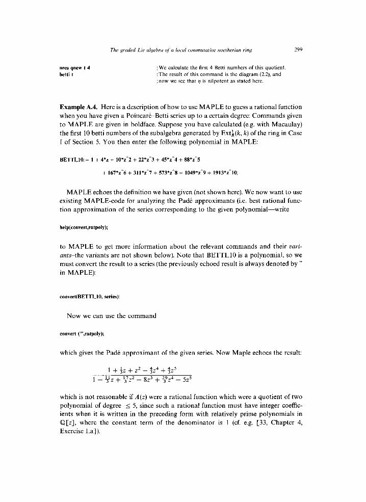
The graded Lie algebra of a local commutative noetherian ring 299
nres qnew t 4 betti t
; We calculate the first 4 Betti numbers of this quotient ;The result of this command is the diagram (2.2), and
;now we see that 9 is nilpotent as stated here.
Example A.4. Here is a description of how to use MAPLE to guess a rational function
when you have given a PoincarbBetti series up to a certain degree: Commands given
to MAPLE are given in boldface. Suppose you have calculated (e.g. with Macaulay)
the first 10 betti numbers of the subalgebra generated by Exti(k, k) of the ring in Case
I of Section 5. You then enter the following polynomial in MAPLE:
BETTI_10:= 1 + 4*2 + lO*z-2 + 22*z-3 + 45*z-4 + 88*z-5
+ 167*z^6 + 311*z-7 + 573*z-8 + 1049*z-9 + 1913*z-10;
MAPLE echoes the definition we have given (not shown here). We now want to use
existing MAPLE-code for analyzing the Pade approximants (i.e. best rational func-
tion approximation of the series corresponding to the given polynomial-write
help(convert,ratpoly);
to MAPLE to get more information about the relevant commands and their uari- urn-the variants are not shown below). Note that BETTI_10 is a polynomial, so we
must convert the result to a series (the previously echoed result is always denoted by ”
in MAPLE):
convert(BETTI_lO, series);
Now we can use the command
convert (“,ratpoly);
which gives the Pad& approximant of the given series. Now Maple echoes the result:
1 + +z + z2 - 32” + $z’
1 - yz + yz2 - 8z3 + qz” - 5z5
which is not reasonable if A(z) were a rational function which were a quotient of two
polynomial of degree I 5, since such a rational function must have integer coeffic-
ients when it is written in the preceding form with relatively prime polynomials in
Q[z], where the constant term of the denominator is 1 (cf. e.g. [33, Chapter 4,
Exercise 1 .a] ).

300 J.-E. Roes
If we continue with MACAULAY calculating more and more coefficients of A it is
not until we reach 14 coefficients that the Pade approximant becomes a nice rational
function with integral coefficients and then we get the same rational function for 15,
16 . calculated coefficients, leading to a prediction for A(z) which is then proved by
hand calculations (cf. Case I in Section 5). Unfortunately what we just said is in this
case only theoretically true, since it is almost impossible in this Case I to calculate
more than 1 l-12 coefficients by MACAULAY (cf. Table 2 below). Instead one must
use the program BERGMAN:
Example A.5. Here is a description of how to use the computer algebra program
BERGMAN of Jiirgen Backelin on e.g. Case I of Section 5: In the case mentioned it is
as we said under Example A.4 rather hard to calculate enough Betti numbers with
MACAULAY. Instead we now calculate the Hilbert series of the non-commutative
algebra A, given by generators and relations.
The program BERGMAN was developed by Jiirgen Backelin in Portable Standard
Lisp (PSL), the same LISP that is underlying the Computer Algebra Program REDUCE.
It should be available by anonymous ftp from our machine 130.237.198.6 as the file
pub/src/bergman.tar.Z. More information can be obtained from: [email protected].
The program is extremely fast, and it calculates the Hilbert series and standard bases
of ideals in both commutative and non-commutative algebras, both in characteristic
0 and in characteristic p. The reason for this program being so fast even in the
non-commutative setting is that it implements in a very clever way some theoretical
results from Backelin’s thesis (1982, University of Stockholm) for calculating the
Hilbert series of the non-commutative ring with monomial relations associated to
a Grobner basis of an ideal up to a certain degree (recall that in the non-commutative
setting, Griibner bases of finitely generated two-sided ideals are often infinite). Earlier
I had mentioned the problem of computiny Hilbert series of non-commutative alge-
bras to Gerhard Pfister at the MEGA conference in Castiglioncello 1990, and
Gerhard Pfister mentioned this problem to Hubert Grassmann in Berlin. H. Grass-
mann developed a nice and useful program GB (in PASCAL originally for IBM PC’s,
but later ported by H. Grassmann to the SPARCSERVER 690MP of the Department
of Mathematics, University of Stockholm) as an extension to his computer algebra
program RAC, but even on the SPARCSERVER it was only possible to calculate
about 7, 8 or may be 9 terms of the Hilbert series in reasonably small examples by
means of GB, which was however extremely useful when we were debugging
BERGMAN. In what follows I just describe how to calculate with BERGMAN the
Hilbert series of the non-commutative algebra A of Case I in Section 1. BERGMAN
can accept MAPLE-form input but also LISP input. We illustrate how to work with
LISP-input in Case I: First create with a text editor the following file:
(setq embdim 4) (LISPFORMINPUT) ((I 1 1)(-l 12)(-l 2 1)) % this corresponds to the element Tf - [T,, T,]

The graded Lie algebra oj’a local commutative noetherian ring 301
((1 1 3)(1 3 1)(-l 2 4)(-l 4 2)) % this corresponds to the element [T,, T,] - [Tz. T,]
((1 2 3) (13 2)) ((1 3 3)) ((134)(143)) ((1 4 4)) (LISPFORMINPUTEND)
Call this file “input”. Then start BERGMAN and write (in char 0)
(ncpbhgroebner “input” “tl” “t2” “t3”)
Here ncpbhgroebner is short for “non-commutative-poincart-betti-hilbert-groeb-
ner” and the files tl, t2 and t3 are the names you give the three files which are created
by the program. The file tl contains the standard basis of the ideal in question, t2 is
the double series of the corresponding monomial ring and t3 is the Hilbert series. (If
the ideal has ajnite Griibner basis for the given ordering of variables-not so in the
case we are studing here-the program stops in the highest degree of a Griibner basis
element, but you can force it to continue up to a higher degree by adding the extra
relation (say): ((1 1 1 1 1 1 1 . 1 1 1)) in the input file.
For the example in question BERGMAN takes 17 minutes and 41 seconds to get
a Hilbert series of 20 terms and MACAULAY takes 56 minutes and 56 seconds to get
only 9 terms (both timings are for the programs running on a Sparcserver 690MP).
More details are given in Table 2. To be quite fair, one should remark that it is not
necessary in each case to calculate to the (bitter) end in MACAULAY since as we have
said earlier it is sufficient to calculate the second horizontal line of the betti numbers
and this can be done in slightly less time in MACAULAY. On the other hand the
timings in the table are for BERGMAN computing in characteristic 0, and for
MACAULAY computing in characteristic 31991 and BERGMAN in characteristic
31991 is faster than BERGMAN in characteristic 0. The table shows the extreme
importance of BERGMAN for our computations in those cases where MACAULAY
needs too much time and memory.
Remark. The calculations with BERGMAN in the table mentioned above do not use
much internal memory (not more than 64 MB). But in some cases you need to go
further and calculate say 30 non-commutative Hilbert series coefficients in embedding
dimension 4. Then you must enter the following command at the beginning of your
input file above:
(set-heap-size 16100000)
This gives you the possibility to use about 128 MB of internal memory for your
calculations. Unfortunately there is a limitation in PSL which prevents you from
using more memory. But there is a program called SL-in-CL which allows you to run
Portable Standard Lisp programs under e.g. Sun Common Lisp and since Sun

302 J.-E. Roes
Table 2
The Hilbert Time in seconds for Time in seconds for Time in secons for
Series of A BERGMAN on a MACAULAY on the same MACAULAY on a
in degrees I Sparcserver 690 MP Sparcserver 690 MP Macintosh SE/30
(40 MHZ Cypress Spare) (192 MB internal memory) (68030, 16.67 MHZ, 8 MB)
2 0.32 <l <l 3 0.37 <l 1
4 0.44 <I 5 5 0.53 1 16 6 0.61 4 75 7 0.73 35 535 8 0.94 372 5020 9 1.21 3416 Prob. imposs. with 8 MB
10 1.56 31724 Impossible 11 2.04 259647 (93 MB int. mem. used) Impossible 12 2.84 Probably impossible Impossible 13 4.47 Impossible Impossible 14 7.49 Impossible Impossible 15 13.9 Impossible Impossible 16 27.8 Impossible Impossible 17 59.3 Impossible Impossible 18 167 Impossible Impossible 19 411 Impossible Impossible 20 1061 Impossible Impossible
Common Lisp can use more memory this enables you to get many more Hilbert series
coefficients.
Example A.6. Here is a “four-lines” MATHEMATICA program for calculating the
deviations of a local ring if you have a corresponding Poincare - Betti series given,
where the third line is the given input.
+I_]: = c[nl = Coefficient [Normal[Series[q[n-11, {z, 0, a+ l}]], fn] qln_1: = IflOddQ[n], q[n-l]/(l +z”n)“c[nl, q[n-11 (1-z*n)*c[nll 4101 = I+%+ 18~~2 +55z^3+ 150zA4+376zA5 +883zA6+ 1966~~7 +4190zA8+8604zA9+ 17107zYO
4Ol
If (on the Macintosh-similar procedures on other machines) you write the preceding
four lines into a cell in MATHEMATICA, select the cell and press enter, you will get
the 10th deviation c[lO]. If you then write
?c
and press enter, you will get all the deviations from the first up to the tenth.
This example is particularly interesting (you see a periodicity in the c[i]‘s), since it
comes from the Hilbert series of the subalgebra A generated by Extfi(k, k) for the ring

The graded Lie algebra of’a local commutatioe noetherian ring 303
in 5 variables with quadratic relations of Case $7 of Section 6. This ring (and minor
variants) is the only one we know of (in 5 variables) where A(z) is irrational, but
holomorphic in the whole interior of the unit circle.
Appendix B. The Lie algebra structure of a ring satisfying Jkt and variants’
Let R be a local noetherian ring with maximal ideal m and R/m = k. Suppose R is
“two-homogeneous” (see [25]); i.e., as a vector space, R is equal to
k@mlm2Qm2/m3Qm3,
and the multiplication on R maps m/m2@m/m2 onto m2/m3. It is proved in [25] that
the sub Hopf algebra of U(gR) = Ext,(k, k), generated by the one-dimensional ele-
ments, gk, is
U(y) = A = T((m/m2)*)/(im((m2/m3)* + (m/m’)*@(m/m2)*)).
It is also proved [25, p. 3301 that U = R @ A* has a structure of a differential graded
R-algebra, such that
BUnm2U c B(mU), z(U) c m2U + BU and H,(U) = k. (B.1)
Also, the minimal resolution Y of k over R is proved to be a free differential U-module,
Y = U@([email protected]), where F = Fz2 is a free graded R-module and dF c m2 Y.
Moreover, if H(U) has trivial Massey operations, it is proved that there is a split
exact sequence of Hopf algebras
k --f T((s&U))*) + U(gR) + U(q) + k.
In [25] the case m4 = 0 is considered. In this appendix we will study some other cases,
which imply that H(U) has trivial Massey operations.
Since TorR(R/m’, k) is the dual of Ext,(R/ mi, k), the property A, (see Section 3) for
a ring R may be formulated in terms of the minimal resolution Y as follows:
BYnm’+‘YcB(m’Y) foriks-1.
Lemma B.l. Suppose R is two-homogeneous. Then R satisjes A, if and only if
ZUnm’+’ Uc B(m’U) foriks- 1.
1 Written by Clas Liifwall.

304 J.-E. Roes
If R satis$es A4 then H(U) has trivial Massey operations, and these may be chosen such
that the Massey product of r cycles is in rn*” U for any r 2 1.
Proof. Suppose R satisfies J%‘~. Since, for allj, Uj is a noetherian R-module, it follows
by the ArtinRees lemma that, for allj, there is an r such that
ZjUnmi+‘Uj c miZjU for all i 2 0.
From above, the minimal resolution Y of k over R has the form Y = U@(U gRF),
where dF c m2Y. Suppose i 2 s - 1 and z E ZjUnmif ’ Uj. Since z is a boundary in
Y and R satisfies JZ7, there is an x E m’Y such that dx = z. Write x as u + v, where
u E m’U and v E m’U @ F. Since dF c m2 Y, the U-component of dv is in mi+2U. Thus,
~-du~ZjUnm’+~ Uj. Continuing in the same manner, we conclude that there is
u EmiU, such that z - du 6 ZjUnmif’f’Uj. Hence, from above,
z - du E mi+‘ZjU c m’BU = B(m’U),
and it follows that z E B(m’U).
To prove the opposite direction, suppose that
ZUnm’+‘U c B(m’U) for i 2 s - 1.
We want to prove that R satisfies JN~. Suppose i 2 s - 1 and y E BYnm’+ 1 Y. We may
write n
Ycu+ C CUjkOfjk9
j=2 k
where u,ujk E U and fjk are basis elements in F, such that the homological degree of
fjk is j. We will prove that y E B(m’Y) by induction on n. For n = 0 this follows by
assumption. Since y is a cycle, u,,~ is a cycle for all k. Since also y E mi+ ’ Y, it follows by
assumption that u,& = d(v,k) for some u,& E m’U. Now, d(fnk) E mY and hence,
y - dj&l”,@hr) E BYnm’+‘Y. \k /
By induction it follows that y E B(m’Y).
Finally, we prove that H(U) has trivial Massey operations if R satisfies &Z4. Since
z(U) c m2U + BU, we may choose cycles in m2U representing a basis for I?(U).
Thus, from above, the product of any two of these cycles is a boundary of an element
in m3U, which defines the Massey products, y(zl, z,), of order two. To define a triple
Massey product, y(zl, z2, z,), we need to consider the cycle
(_ l)Zlfl zly(z2, z3) + ( - 1)z1+z2~(zl, z2b3.

The graded Lie algebra of a local commutative noetherian ring 305
This cycle is in m5U and hence, from above, it is a boundary of an element in m4U.
This process may be continued and we get the result. 0
We may now apply the results in [ZS] to obtain that if R satisfies A4, then gR is
a semi-direct product of PJ with a free Lie algebra L(M), where M = (&(U))* is
a certain q-module. A priori, the action of q on L(M) restricted to M, may contain Lie
products of elements in M (see [30, Remark 1 after Theorem 41). However, if
R satisfies Jz’~, the y-module structure of M completely determines the action of ye on
L(M). For the proof we will use the same technique as in [24] (where some other cases
are studied).
Theorem B.2. Suppose R is two-homogeneous and suppose there is a t 2 2, such that
U = R @ A* satisfies the following three conditions
(1) z”U c m’U + BU,
(2) BUnm’U c B(m’-‘U),
(3) ZUnm’+’ U c B(m’U) for i 2 2t - 2.
These conditions are satisfied for t = 2 if R satis$es A3. Let gR be the Lie algebra of
R and n the sub Lie algebra of gR generated by gk. Then there is an n-module M, such
that gR is the semi-direct product of v] with the free Lie algebra L(M) equipped with the
induced y-module-algebra structure.
Proof. By (B.l) and Lemma B.l, the conditions are satisfied if t = 2 and R satisfies
Ma. The conditions imply that H(U) has trivial Massey operations, which may be
chosen such that the product of r cycles is in rnrtmr+’ U for any r 2 1. The minimal
resolution Y of k over R has the form U Ok T(W), where W = sfi(U) and f(W) is the
tensor algebra on W equipped with the shuffle product. The differential d on Y satis-
fies the following for v E W@“,
due &(mrt-“+’ u Ok w@” ~ ‘), I= 1
where W@’ = k. We have that U(gR) is equal to Horn,,, Y, k) as vector space, and the
product is given as composition in HHom,( Y, Y). To get the result, it is enough to
consider f E n1 = Horn,,, Y,, k) and g E M = Homk( W, k) (g is considered to be zero on
the other components of Y) and prove that [g, f ] E M. It is possible to define a lifting
F E Z Hom,(U, U) off (see [24, p. 3091). Next, we define F on W. Using condition (2),
we then prove in the same way as in [24, p. 3073, that F may be defined such that
F(W) c W@m’-’ U. Finally, we define F E Z Horn,,, Y, Y) degree by degree, first on
f(W), then using the derivation rule, on all of Y.
From the analysis in [24, p. 3081 or from the proof of Lemma 7 in [30], it follows
that [g, f ] is equal to go F restricted to

306 J.-E. Roes
Hence, we are done if we can define F such that
(the tensors to the left are of length at least two). In fact, we will prove
by induction over the homological degree. For i = 1 this is true. Suppose it is true for
< i and let u E W@' + ‘. From above we have -
due ~(mr+‘(r-l)UO,W~‘~r). r=O
By induction and the derivation rule, this is also true for F(dv). The component of
F(du) in m’U Ok W@’ may be written xx,,@ y,,, where (y,} is a basis for W@“’ and
x, E m’U. Since F(du) is a cycle, x, is a cycle for all ~1. Hence, by condition (2), there are
a,, E m’-‘U and u, E W such that x, = da, + du, and we get
Now we look at the “highest” component again. We get rid of this term by subtracting
d( Cb, 0 z,), where b, E m 2t- 2U and z, E W@’ ~ ‘. Here we have used condition (3) for
i = 2t - 2. Finally we get that F(du) is a boundary of an element of the right type,
which we choose as the definition of F(u). 0
From now on we assume that R is graded; i.e.,
R = R,@R,@R,@... z Gr(R) = kQmlm2@m2/m3@m3/m4@... .
The differential d on the graded free complex U = R@A* satisfies d: Ri@(A*)j +
Ri + 1 @ (LI*)~_ 1. Dualizing we get a graded complex, R* @A, which is a graded free
complex over A. We say that (R*)‘@ A’ has homological degree i and internal degree
i + j. The differential maps (R*)‘@ A’ to (R*)‘- 1 @ A’+ ‘. We can now reformulate the
conditions in Theorem B.2. and describe the y-module M.
Theorem B.3. Suppose R ‘u Gr(R) and suppose there is a t 2 2 such that
H’(R*@A)=OforO<i<t and i>2t-2.

The graded Lie algebra of a local commutatiae noetherian ring 307
Then the conditions in Theorem B.2 are satis$ed and
Zf-2
M = @ s’-‘H’(R*@A)
i=f
as right A-modules, where s shifts the internal degree. Moreover, R satisjes JV~ if and
only [f
H’(R*@A)=O for i2s.
Proof. Using the graded structure of U, it follows that BUnm’+‘U c B(m’U) for
i 2 1 and from this, the conditions (l)-(3) in Theorem B.2 are easily proved. We will
now examine the A-module M. If f~ H,(U, k), then the lifting F: U + U used in the
proof of Theorem B.2 is defined as the R-linear extension of (1 of) o A : A* + A*. The
dual of F is right multiplication by f on R*@A. As was noticed in the proof of
Theorem B.2, [g,f] = go F forfE y and g E M. This gives the claim about the A-
module structure of M. The occurrence of the operator sip ’ in the formula for M is
motivated as follows. We have (M*), = H, _ 1 (R @ A*), where the homology degree is
the “A*-degree”. The internal degree of H’(R* @A) is i step higher than the A-degree.
Hence the formula follows, since (siplHi(R* @ A))” = H’(R* @ A)“+‘- ‘.
The last claim follows from Remark 3.6 or from Lemma B.l and the fact that, in the
graded case, BUnm’+‘U c B(m’U) for i 2 1. 0
Theorem B.4. Let R = k[x, . . , x,]/(fi , . . ,fi, gl, . . . , gs), wherefi, gi are homogene-
ous polynomials with deg(A) = 2, deg(gJ 2 3, and let S = k [x, . . . , x,]/(fi, ,f*). Suppose R satisjes 9t for some t 2 2; i.e.,
H’(R*@A)=O for i#O,t- 1
(see also Section 3). Let B = U(gR) = Ext,(k, k) and A = U(q), where v] is the sub Lie
algebra qf gR generated by gi. Then we have the following formula for the Poincar6 series
ofR:
P,‘(x, y) = (1 - (- x)-‘+‘)/A(xy) + (- x)-*+‘Hd - xy). 03.2)
Moreover, we have the following formulas, where A and B are considered as graded by
the homological degree only:
Torf(k, k)” N (S,)*,
Torfl(k, k)‘+l N Tor~(k,k)“‘lO(S,+,-l/R,+t-l)*,
Torf(k, k)j = Tori(k, k)j@Torf+,_ ,(k, k)j+‘-’ for j # n + 1.
(B.3)
03.4)
(B.5)
308 J.-E. Roes
In particular, we have
Torf(k, k)’ N (RI)*, Torf(k, k)* N (St/R,)*,
Torf(k, k)j N Tor:(k, k)jifP2 for j 2 3,
Tor!(k, k)’ cx (R2)*, To$(k, k)3 = (SI +JR1 +J*,
Tort(k, k)j N Tor:+t(k, k)j+fP2 fbr j 2 4.
Proof. To get the first formula, we consider the complex R* @A in each internal
degree. This is a finite complex of finite-dimensional vector spaces and we may use the
technique of taking the alternating sum of the dimensions, before and after homology
is applied. A simple computation gives, A(z)H,( - z) = 1 - ( - l)‘~‘~~M(z), where
M = s’-‘Htm ‘(R* @A). But, as a vector space, B is equal to A@ T(M). Hence,
P,(x, y) = A(xy)/(l - yce2M(xy)), and the result follows.
To get the other formulas, we apply first the Hochschild-Serre spectral sequence to
the split extension of Hopf algebras
k+T(M)+B+A+k
and get
Torg(TorrCM)(k, k), k) =E= Torfl(k, k).
The spectral sequence degenerates, since the sequence splits and d2 is given as the cap
product by the second cohomology class defining the extension. Thus,
Torf(k, k) N Tor!(k, k) 0 Tar/_ 1 (M, k).
It remains to compute Tori_ ,(M, k). Put I/ = H’- ‘(R* @ A). Let P be a free resolu-
tion of k over A and consider the spectral sequence associated to the double complex
(R* @ A)OAP. Since
‘k ifq=O,
H4(R* @A) = ( V if q = t - 1,
,O if q#O, q#t-1,
we get a long exact sequence
. . . -+Tor~-4-t+l(V,k)+RT +Tor$(k,k) +Tor$_4-t(V,k) +Ri*_l + ....

The graded Lie algebra of a local commutatiae noetherian ring 309
This is a sequence of (upper) graded modules, where RT has upper degree i. Hence,
Tort(k, k)j ‘v Tortm4_,( F’, k)j for j > i
and, since V = V” implies Tor~-_r+I(V, k)’ = 0, we get an exact sequence,
0 --+ R,+ -+ Tort (k, k)’ + Tort_4_,(V, k)’ + 0.
Now by [25, Corollary 1.21, we get Tort (k, k)’ % ST. Hence,
Tor$(M, k)j = TorA(V, k)j+rm2 5 Tort+4,,(k, k)j+t-2 forj > i + 2,
Torf(M, k)i+l = 0, Tort (M, k)‘+2 = Tort (I’, k)i+t ‘v (Si+t/Ri+,)*,
and the result follows. 0
Remark B.5. We have in fact that A and B are bigraded, where A is concentrated on
the diagonal. Thus, To?(k, k) has three degrees. It is possible to read off the third
(internal) degree from the formulas given in the theorem, using the fact that the
internal degree of Rf (and SF) is i. Thus, e.g., (B.5) may be split up into the following
formulas:
Tort(k, k)jj = Tort (k, k)“,
Torfl(k, k) j,j+tv2 = ~~~;+,_~(k, k)j+t-2.j+r-2,
Tot-f (k, k)jq = 0 for 4 # j,j + t - 2.
Remark B.6. When m3 = 0, V is the third syzygy in a minimal resolution of k over A.
Hence, in this case we have
Tort(V, Q)’ = Torf+33k Q)'
for any left A-module Q. Using this, we get an alternative proof of Theorem 4.1:
Suppose q ” is free. The Lie algebra gi ’ is a sub Lie algebra of the Lie algebra
generated by M and rl “. Hence, it is enough to prove that this Lie algebra is free,
which follows if we can prove that rj ” acts freely on M. But this is true since
Tory’V”‘(V, k) N Torf(V, A@ut,>t,k) N Tori(k, A@ucq>t,k)
II Tory(q”)(k, k) = 0.
We will now turn to a detailed study of the complex R*@ A, in the case when
R = k[x, y, z, . . . ]/(quadratic polynomials). We prove that if) R,,I I 2 for some IZ 2 2,
then H’(R* @A) = 0 for i 2 n; i.e., R satisfies JZ,,. In particular, R satisfies A3 if
lR31 I 2.
The following lemma was shown to me by Rickard Bogvad.

310 J.-E. ROOT
Lemma B.7. Suppose n is a graded Lie algebra, A = U(n), and a E A,. If ax = 0 for
some 0 # x E A, then x = ayfor some y E A and a2 = 0 in r]. Similarly, rfxa = Ofor some
0 # x E A, then x = ya for some y E A and a2 = 0 in n.
Proof. This easily follows from the Poincare-llirkhoff-Witt theorem, or from Lemma
B.8 below. 0
Lemma B.8. Suppose n is a graded Lie algebra, A = U(g), and suppose aI,. . . , a, E A’
are linearly independent elements. The solutions to xlal + . + x,a, = 0 (or
alxl + . . + a,x, = 0) over A are generated by the solutions to the same equation over
the subalgebra A0 of A generated by a,, . . , a,,. Moreover, the minimal relations in A,,
determine a generator set for the solution space of the equation. The dimension of the
solutions to xlal + . + x,a, = 0 in degree i is equal to the dimension of the solutions
to alxl + .... + a,x, = 0 in degree i.
Proof. The first claim follows since A,, is equal to the enveloping algebra of the
Lie algebra generated by aI, . . , a,, and hence A is free over AO. The rest of the
claims follow from the interpretation of Tort@, k), valid for any augmented
k-algebra A. 0
Theorem B.9. Suppose R = k[x, y, z, . . . ]/(quadratic polynomials) and suppose
1 R,) I 2~for some n 2 2. Then R satisfies A,,.
Proof. We will separately study the cases 1 R, 1 = 1 and 1 R, 1 = 2.
IR,J = 1: The matrix for d,:R,* @ A + R,*_ 1 @A is given by a column matrix
(a,,..., a,,,), where a,, . , a, E A’. We may suppose a = a, # 0, since the complex is
minimal. If ker(d,) = 0 then R,, , = 0 and the result follows. Suppose 0 # b E ker(d,).
Then ab = 0 and hence, by Lemma B.7, a2 = 0. This implies that R is non-artinian,
since we may choose a presentation of R as k[x, y, z, . . . ]/(relations), where a is dual
to x, such that x2 does not occur in the relations. In the same way we see that as = 0
and furthermore, if a and a2 are linearly independent, we may choose a presentation of
R with two variables x, y such that x2 and y2 do not occur in the relations. Hence, x”,
y” # 0 in R and so lR,,l 2 2, which is a contradiction. It follows that we can find
a basis for A”, such that the matrix for d, is the column (a, 0,. . . , 0). Now, ker(d,) is
generated by a, and hence the complex has the form
(4 (0) . ..- A-ALA”‘,
and is acyclic according to Lemma B.7.
I R, I = 2: We first prove that, after a base change, the matrix for d, has two linearly
independent elements, a and b, in the first row. Indeed, if this is not true, we may
The graded Lie algebra of a local commutatice noetherian ring 311
assume that the first row is (a, 0), where a # 0, the second row is (0, a) and the other
rows are zero. But then a2 = 0, and we can choose bases, such that the first two
columns in the matrix for d,_ 1 are the same as the matrix for d,. Continuing in this
manner, we finally end up with (a, a, ) as the matrix for dI, which is impossible.
Next, we divide the case study according to the value of dim(R,+ i). This is bounded
from above by dim(N), where N = {(x, y) E A’ x A’ 1 ax + by = 0}, and, by Lemma
B.8, this dimension is equal to the number of linearly independent relations between
a2, b2, [a, b]. Th e case a2 = b2 = [a, b] = 0 is impossible, since then R may be
presented as k [x, y, . . ] /(relations), where x2, y2, xy do not occur in the relations, and
this implies that 1 R, 1 2 3. Hence dim(R,+ r) I 2.
Suppose R,+ 1 = 0. We have to prove that ker(d,) = 0. Suppose (0,O) # (x, y) E
ker(d,). Since R is artinian, it follows from Lemma B.7 and the argument above that
x and y are linearly independent. Also, by Lemma B.8, x and y belong to the
subalgebra of A generated by a and b. By the Poincare~Birkhoff-Witt theorem, it
follows that all elements in the matrix for d, also belong to this subalgebra. Again,
since R is artinian, no row in the matrix for d, can have exactly one zero element.
Hence we can find a basis such that the second row in the matrix ford, is (b a) and the
other rows are zero. But if x0, y, E A’ are the first two elements in the first row in the
matrix for d,_ 1, we get that xoa + y, b = 0 and y,a + x0 b = 0. From this it easily
follows that some linear combination of a and b has square zero, which, as above, is
impossible.
Suppose dim(R,+ r) = 1 (the case dim(R,+ 1 ) = 2 is treated similarly). Let (x,, y,) be
a basis for N. By Lemma B.8, we know that x0 and y, belong to the subspace of A’
generated by a and b. If x0, y, are linearly independent, the same lemma shows that
(a, b) is a basis for {(x, y) E A’ x A’ 1 xx0 + yy, = 0). But then we may assume that all
except the first row in the matrix for d, are zero. This implies, by Lemma B.7, that the
elements in the first column of the matrix ford,_ 1 are multiplies of both a and b, which
is impossible. Hence x0 and y, are linearly dependent. Since ax0 + by, = 0, Lemma
B.7 gives that a linear combination of a and b has square zero. Hence R is non-artinian
and by the first part of the proof we must have, 1 Ri 1 = 1 for i 2 n + 1. After a base
change, we may assume that a2 = 0 and the matrix for d, has first column equal to
(a, 0, . , 0). The complex R* @A in homological degrees 2 n - 1 has the following
form,
\O hml (4 -+ A-!~!-.+A---+... -*J+p- (0) . . . At?,+1
The complex is exact in homological degrees 2 IZ + 1, by Lemma B.7. Suppose that
(x, y) E ker(d,), where y # 0. By Lemma B.7 and since dim(R,+ r) = 1, hi is a multiple
of a for all i. From the first part of the proof it follows that m 2 1, and hence we may
assume that the second column is (b, a, 0, . . . , 0). But {(x, y) E A’ x A’ 1 xb + ya = 0)

312 J.-E. Roes
is generated by (0, a). Hence, the first column in the matrix for d,_ 1 must be zero,
which is impossible, Thus, the complex is acyclic.
This case does occur. If R = k[x, y, z]/(xy - z2, y2, xz, yz), then R* @ A has the
form above in degrees 2 2, where m = 2, b, = a, b2 = - c and a, b, c is the basis dual
to x, y, z. 0
Remark B.10. Examining the proof above, we see that we in fact have proved that one
of the following cases hold if 1 R, 1 I 2 (and the relations are of degree two in R),
(1) R,+I = 0, (2) ( Ri ( = 1 for i > n,
(3) lRil=2fori>n.
The fact that 1 Ril 5 2 for i 2 n follows from the Macaulay inequality (cf. [32]).
However, the result that R is non-artinian if R,, 1 # 0 seems to be new, at least the
proof method. The result above for IZ = 2 was obtained by Backelin [6, Theorem 4.81
and his methods may be used to get an alternative proof for a general n.
We may now apply Lemma B.l and Theorem B.9 to obtain that R satisfies A3 in
Case III, VI and VII of Section 5. In Case IV this is trivially true. The other cases may
be handled by explicitly writing down the complex R* @ A, and showing (using
Lemmas B.7 and B.8) that its augmented homology is concentrated in degree two. In
Case VIII, R does not satisfy J.&‘~. However, in this case the augmented homology is
concentrated in degree three; i.e., R satisfies Yb. Thus, Theorem B.4 may be applied.
In this case, it is in fact possible to write down an explicit resolution of k over A, and
a presentation of Ext,(k, k).
Here is the complex R* @A in Case II (a, b, c d is the basis for A’ dual to X, y, z, u):
- R;@A - R;@Ap . . .
I 0 0 Oh-a c
0 0 c a -d
cdh0 a I
\’ c-d ’ ’ -‘I RTOA(a b c d)
, -A
It is easy to prove that the homology is zero in degree 2 3, using Lemma B.7 and the
relations [b, c] = 0 and d2 = [c, d].

The graded Lie algebra of a local commutative noetherian ring
Here is the complex in Case VIII:
. . .
A4 (0 b C d) - A.
Again, it is fairly easy to see that the augmented homology is concentrated in degree three and that H3(R*0 A) is generated by (( - d - a - c)b, (a + c)‘, ab,
(B.6)
- (a + c)b) E A4. Also, H 3(R* 0 A) is isomorphic to A/bA as right A-modules.
Thus, by Theorem B.3, we have the following presentation of B = ExtR(k, k):
B = k(a, b, c, d, e>l(a” - [a, bl - Cb, cl, b2, Cb, cl - d2,
CG cl - Cb, 4, [a, 4, Cc, 4, Cb, el)
where a, b, c, d has homological and internal degree 1, while e has homological
degree 3 and internal degree 5.
The resolution of k over A in homological degrees I 3 is obtained from (B.6). By
the above, the rest of the resolution may be calculated. The result is
0 (-d-a-c)h
(; ‘“;‘)‘) . . (,” -(a;c)i)Ae44BAe4 - Aess@Ae56 P 5 A4,
where eij is a generator of homological degree i and internal degree j. Hence,
Torf(k, k)’ = R;,
1 Tor”(k, k)i+l 1 = 1 for i 2 4,
TorA(k, ky’ = 0 for j > i + 1.
314 J.-E. Roes
Moreover, by Theorem B.4 with t = 4, we have
P,(x, y)_’ = (1 - l/x2)/A(xy) + H( - xy)/x2,
and
TorB(k, k)’ = RF,
I Torf(k, k)‘+ 1 1 = 1 for i 2 4,
lTorB(k, k)i+21 = 1 for i 2 1,
Torf(k, k)j = 0 for all other values of i and j.
In particular, ) Tort(k, k)46 ( = 1 (cf. Remark B.51, which corresponds to the relation
[b, e] = 0 in the presentation of B above.
Note added in proof. The problem about commuting n x n matrices in Section 2 has
been solved for n = 4 in [36]. Further relevant examples and results related to our
own paper are given in [37] and [38].
References
[1) D.J. Anick, A counterexample to a conjecture of Serre, Ann. of Math. 115 (1982) l-33; Correction Ann. of Math. 116, p, 661.
[2] L.L. Avramov, Local rings over which all modules have rational Poincare series, J. Pure Appl.
Algebra 91 (1994) this volume.
[3] L.L. Avramov and Y. Felix, Espaces de Golod, in: H.R. Miller, J.-M. Lemaire et J.-C. Thomas, eds.,
Theorie de l’homotopie, Asttrisque 191 (1990) 29934.
[4] L.L. Avramov, A.R. Kustin and M. Miller, Poincare series of modules over local rings of small
embedding codepth or small linking number, J. Algebra 118 (1988) 1622204.
[S] L.L. Avramov and G. Levin, Factoring out the socle of a local Gorenstein ring, J. Algebra 55 (1978) 74483.
[6] J. Backelin, A distributiveness property of augmented algebras, and some related homological results,
part of thesis, Stockholm, 1982.
[7] J. Backelin, Golod attached rings with few relations II, Reports, No. 20, Department of Mathematics, University of Stockholm, 1982.
[S] J. Backelin and R. Froberg, Poincare series of short artinian rings, J. Algebra 96 (1985) 4955498.
[93 D. Bayer and M. Stillman, MACAULAY, version 3.0 for Sun 4 (SPARC), Sun 3, Macintosh, Amiga, etc. available by anonymous ftp from math.harvard.edu (198991992).
[lo] F.R. Cohen, J.C. Moore and J.A. Neisendorfer, Torsion in homotopy groups, Ann. of Math. 109
(1979) 121-168. [I l] Y. Felix, S. Halperin, C. Jacobsson, C. Lofwall and J.-C. Thomas, The radical of the homotopy Lie
algebra, Amer. J. Math. 110 (1988) 301-322. [12] R. Froberg, Determination of a class of Poincare series, Math. Stand. 56 (1975) 29939.
[13] T.H. Gulliksen and G.L. Levin, Homology of Local Rings, Queen’s Papers in Pure and Applied
Mathematics Vol. 20 (Queen’s University, Kingston, Ont., 1969).
The graded Lie algebra of a local commutative noetherian ring 315
[14] S. Halperin, The non-vanishing of the deviations of a local ring, Comment. Math. Helv. 62 (1987)
646653.
[lS] C. Jordan, Reduction d’un reseau de formes quadratiques ou bilineaires, J. de Math. (6) 2 (1906)
403-448.
[16] C. Jordan, (Euvres de Camille Jordan, ed. Jean Dieudonnt, Tome III (Gauthier-Villars, Paris, 1962).
[17] A.R. Kustin and SM. Palmer, The Poincare series of every finitely generated module over a codimen-
sion four almost complete intersection is a rational function, J. Pure Appl. Algebra, to appear.
[18] J.-M. Lemaire, Algebres Connexes et Homologie des Espaces de Lacets, Lecture Notes in Mathemat-
ics, Vol. 422 (Springer, Berlin, 1974).
[19] G. Levin, Local rings and Golod homomorphisms, J. Algebra 37 (1975) 266289.
[20] G. Levin, Lectures on Golod homomorphisms, Reports, No. 15, Department of Mathematics,
University of Stockholm, 1976.
[21] G. Levin, Large homomorphisms of local rings, Math. Stand. 46 (1980) 2099215.
1221 G. Levin, Finitely generated Ext-algebras, Math. Stand. 49 (1981) 161-181.
[23] C. Lofwall, The Yoneda Ext&algebra for an equi-characteristic local ring (R, m) with m3 = 0, unpub-
lished manuscript, circa 1976.
[24] C. Lofwall, On the homotopy Lie algebra of a local ring, J. Pure Appl. Algebra 38 (1985) 3055312.
[25] C. Ldfwall, On the subalgebra generated by one-dimensional elements in the Yoneda Ext&algebra, in
J.-E. Roos, ed., Algebra, algebraic topology, and their interactions, Lecture Notes in Mathematics,
Vol. 1183 (Springer, Berlin, 1986) 291-338.
[26] C. Liifwall and J.-E. Roos, Cohomologie des algebres de Lie graduees et series de Poincare&Betti non
rationnelles, CR. Acad. Sci. Paris Ser. I Math. 290 (1980) A7333A736.
[27] J.W. Milnor and J.C. Moore, On the structure of Hopf algebras, Ann. of Math. 81 (1965) 21 l-264.
[28] J.-E. Roos, Relations between the Poincare-Betti series of loop spaces and of local rings, Lecture
Notes in Mathematics, Vol. 740 (Springer, Berlin, 1979) 2855322.
[29] J.-E. Roos, On the use of graded Lie algebras in the theory of local rings, in: R.Y. Sharp, ed.,
Commutative algebra, Durham 1981, London Mathematical Society Lecture Note Series, Vol. 72
(Cambridge University Press, Cambridge, 1982) 204-230.
[30] G. Sjodin, The Ext-algebra of a Golod ring, J. Pure Appl. Algebra 38 (1985) 337-351.
[31] L. Smith, Split extensions of Hopf algebras and semi-tensor products, Math. Stand. 26 (1970) 1741.
[32] R. Stanley, Hilbert functions of graded algebras, Adv. in Math. 28 (1978) 57783. [33] R. Stanley, Enumerative Combinatorics, Vol. 1 (Wadsworth & Brooks/Cole, Monterey, CA, 1986).
[34] J. Wisliceny, Eine Methode zur Konstruktion nilpotenter Liescher Algebren, Math. Nachr. 118 (1984)
209-214.
1351 J. Wisliceny, Konstruktion nilpotenter associativer Algebren mit wenig Relationen, Math. Nachr. 147
(1990) 75-82.
[36] F. Hreinsdbttir, A case where choosing a product order makes the calculation of a Groebner basis
much faster, 1993 (submitted to J. Symbolic Comput.).
[37] J.-E. Roos, Commutative non-Koszul algebras having a linear resolution of arbitrarily high order.
Applications to torsion in loop space homology, C.R. Acad. Sci. Paris Ser. 1. Math. 316 (1993)
1123-1128.
1381 J.-E. Roos, On computer assisted research in homological algebra, in: Proceedings of the Inter-
national IMACS Symposium on Symbolic Computation, Lille (1993) 74-84.