a computer method for calculation of the complete … · of the complete and incomplete elliptic...
TRANSCRIPT

Office of Naval Research
Department of the Navy
Contract Nonr 220(43)
A COMPUTER METHOD FOR CAlCUlATION OF THE COMPLETE AND INCOMPLETE
ElLIPTIC INTEGRALS OF THE THIRD KIND
K" " arman
by
D. K. Ai and Z. l. Harrison
Hydrodynamics Laboratory
Laboratory of Fluid Mechanics and Jet Propulsion
California Institute of Technology
Pasadena, California
Report No. E-ll 0.3 February 1964

Office of Naval Research Department of the Navy Contract Nonr 220(43)
A COMPUTER METHOD FOR CALCULATION
OF THE COMPLETE AND INCOMPLETE
ELLIPTIC INTEGRALS OF THE THIRD KIND
by
D. K. Ai and Z. L. Harrison
Reproduction in whole or in part is permitted for any purpose of the United States Government
Hydrodynamics Laboratory Karman Laboratory of Fluid Mechanics and Jet Propulsion
California Institute of Technology Pasadena, California
Report No. E-110. 3 Approved by: T. Y. Wu
A.J. Acosta
February 1964

ABSTRACT
Numerical approximations and a Fortran IV program are given
for the calculation by an IBM 7090 computer of the complete and incom
plete elliptic integrals of the third kind. In its present form results are
limited to six decimal places, but the method is valid for all values of
amplitude cp, modulus k and real values of the parameter a. 2. For
the purpose of completeness, adaptations of other programs for complete
and incomplete elliptic integrals of the first and second kind are also pr e
sented.

TABLE OF CONTENTS
Abstract
List of Symbols and Definitions
1. Introduction
2. Complete Elliptic Integrals of the Third Kind
3. Incomplete Elliptic Integrals of the Third Kind
4. Appendices
A. Approximate Functions for the Complete Elliptic Integrals of the First and Second Kind
B. Evaluation of the Incomplete Elliptic Integrals of the First and Second Kind
C. Flow Charts and Subroutines
References
Page
1
3
7
17
19
24
27

LIST OF SYMBOLS AND DEFINITIONS
k,k'
y or cp
F(cp, k), E(cp, k),
II(cp,a. 2 ,k)
K, E and II(a. 2, k)
parameter in the elliptic integral of the third kind.
modulus and complementary modulus, 0 ~ k 2 ~ 1 and k' = Jl - k2 .
argument of the elliptic integral 0 < y~ l, O<cp~~
elliptic integrals of th e first, second and third kind respectively, where
and y
1 dt II(cp,a.2, k) = s
0 1 - a.2 t2 V(l - t2 H 1 - k2 t2)
complete elliptic integrals of the first, second and third kind respectively, where
.. 1 1r 12 K = K(k) = { d t = (' de
jo J(l-t2)(1 -k2 t2 ) jo Jl-k2 sin2 e
1 ,1r 12 ,....v 2 2 5 r----E = E(k) = \ 1 - k t d t = J 1- k 2 sin2 e de Jo I- t 2 o
1
II(a.2' k) = s 0
1
,'IT 1?.
= '~o 1 - a.2 :in2 e
dt
dB

Z(q>,k)
A (q>,k) 0
approximation functions of complete elliptic integrals of the first and second kind.
Jacobian Zeta Function.
E Z(q> , k) = E(q>, k) - K F(q>, k)
Heuman's Lambda Function.
A (q>,k) = ~ {EF(q>,k') + K( E(q>,k')- F(q> , k')]} 0 'IT

l. Introduction
There are tables of the elliptic integral of the third kind, [l] , [z] ':';
these tables are somewhat tedious to use because of the limited number
~:~ :::;: of entries and range necessary in a three parameter tabulation. Either
cross plotting or non-linear interpolation are necessary to obtain values
of IT within the range of the tables and furthermore, values of the integral
outside the range of the tables must be calculated from cumbersome
addition formulae as well as interpolation. These methods are undesir-
able when very many values of these integrals are needed and completely
impractical for adaptation to computer use.
Our interest and need of evaluating these elliptic integrals arise
1n a study of free-streamline potential flows. This problem requires
the numerical integration of expressions involving II as well as evaluat-
ing all of the elliptic integrals many times. Since these calculations
are performed on an IBM 7090 digital computer, it is necessary to have
computer methods of evaluating these elliptic integrals as needed.
Three subroutines have been written in Fortran IV language to ac-
complish this result: the complete elliptic integrals of the first and sec-
ond kind K and E; the incomplete elliptic integrals of the first and sec-
ond kind, F(cp, k) and E(cp, k); and most especially th e complete and in
complete e lliptic integrals of the third kind, II(a. 2 , k) and I1(cp,a. 2 , k)
':' The numbers in brackets refer to references at the end of the text. ,;,,:, In Ref. [l] for example, - 1 <a. z < l and in Ref. [z] - l <a. z < 0.

respectively. The first two of these programs closely follow methods
outlined by others, Refs.[3] and[4] and are detailed in Appendices A
and B respectively.
The present programs are written in single precision arith-
metic since that accuracy is sufficient for our calculations. The accuracy
of the program for K and E, which uses the approximate formulae
given in Ref. [3] , would not be improved by converting to double pr eci-
sian arithmetic. The remaining subroutines use series representations
and consequently their accuracy can be improved by carrying more signi-
ficant figures. All programs are, in their present form, accurate to six
figures with the following exceptions: when k sin cp > 0. 9, E(cp, k) and
F(cp,k) lose accuracy; when k 2 > 0.9 or la. 2 -ll< 0.1, II(cp,a. 2 ,k) and
:::c II(a. 2
, k) lose accuracy. Four figure accuracy is guaranteed except
k sin cp> 0 . 9999 or !1- a. sin cpj< 0. 0001. Whenever the accuracy is less
than six figures, comments are printed and indicators are set to inform
the user of this loss in accuracy.
The flow chart and the Fortran IV program listings are in-
eluded in Appendix C.
>:< This result is because the accuracy in computing (1- k sin cp), (l-a. 2 ), and (1-a. sin cp) decreases as a. and k approach unity as cp tends to Tf /2.
z

2. Complete Elliptic Integrals of the Third Kind
The complete elliptic integral of the third kind, i. e. ,
1
TI(a.Z' k) = s 0
l dt rrh.
= \ 1 - a.2
1
s in2 f)
dfJ
depends on the two parameters a. 2 and k. Considering only real
values of a. 2 , the ranges of these parameters are
Some special cases of a. 2 and k are as follows:
a) k = 0; the integral can be integrated in closed form and is
rr 1 a.2 < l 2 ~ n (a. 2, o) = 00 a.2 = 1
;!< a.2 > 0 1
b) k = l; rr (a. z, l) = 00
c) a.2 = 0; rr (O, k} = K
d) a.2 = ±k; Il(±k,k) 1
[rr+2(l 'fk}K] = 4(1 =fk}
e) a.2 = k2; rr (k2, k) E ---1- k 2
f) a.2 = l; Il(l,k} = 00
The remainder of the values of a. 2 and 0 < k 2< 1 can be classified
into four cases as shown in Fig. l.
For a. 2 > 1, the integral is interpr eta ted by its Cauchy s principal value.
3
( l }
(2}
( 3)
(4)
( 5)
(6)
(7)

Case I, 0< -a. 2 < oo
Circular cases;
Case II,
Case III,
Hyperbolic cases;
Case IV,
-oo 0 1.0 00
------- I ------+1 ..... >----- lli -----~-1 ...... .___ li -~--+-1------ .nz:: --
Figure 1
The integral, II(a. 2 , k), can be evaluated in terms of elementary _,,
functions and Heuman's Lambda function'''
A (rp,k) =3_ {EF(rp,k') + K[E(rp,k')- F(rp,k')]} 0 1T
for the circular cases (I and II) or of the Jacobian Zeta function
E Z(rp,k) = E(rp,k)- K F(rp,k)
or KZ(rp,k) = KE(rp,k)- EF(rp,k)
for the Hyperbolic cases (III and IV).
,:, These definitions and formulae can b e f o und in R e f. [5] .
(8)
(9)
(9a)
4
5
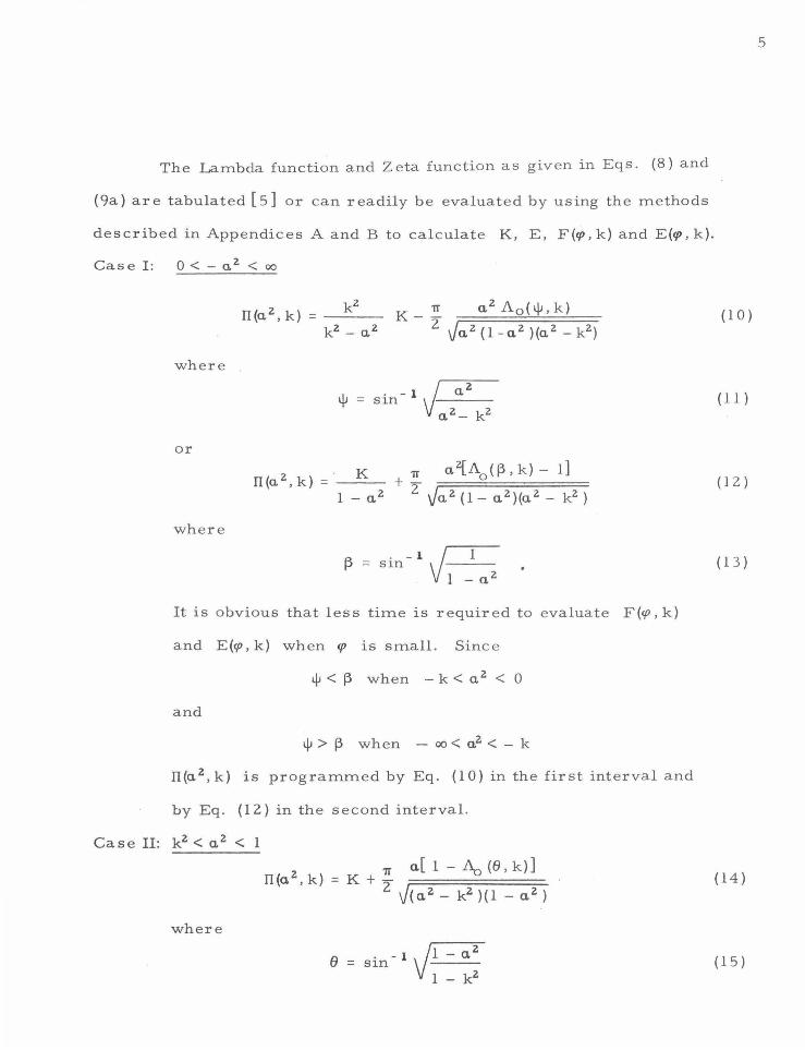
The Lambda function and Zeta function as given in Eqs. (8) and
(9a) are tabulated [5] or can readily be evaluated by using the methods
described in Appendices A and B to calculate K, E, F(cp, k) and E(cp, k).
easel: 0<-a. 2 <oo
K- ~ a.zAo(l!J,k)
2 Ja.z(l-a.Z}(a.2.-kZ) ( 1 0)
where
( 11 )
or
(] 2)
where
(.t .-lt tJ = s1n 1 - a. z
( 13)
It is obvious that less time is required to evaluate F(cp, k)
and E(cp,k) when cp issmall. Since
l.jJ < 13 when - k < a. 2 < 0
and
l.jJ > 13 when - oo < a.2 < - k
II(a. 2 , k) is programmed by Eq. (10) in the first interval and
by Eq. ( 12) in the second interval.
Case II: k 2 < a. 2 < 1
1T a.[ 1 - ~ (B, k)] =K+-
2 J ( a. z - kz ) ( 1 - a. z ) ( 14)
where
a · -1~-a.Z u = s1n 1 - kz
( 15)

or
a. ~ (€., k)
where
In the ranges
k<a. 2 <l ()<€,
and when
k2 < a. 2 < k ' () > €.
In the program, Eq. (14) is used for () < €. and Eq. (16) is
used for () > €..
Case III: 0 < a. 2 < k 2
where
. -1 a. R. = s1n t-' k
Case IV: l < a. 2 < oo
TI(a.z,k)= _ a.KZ(A,k)
v(a.z- l )(a.z- kz)
where
A = sin - 1 l a.
The flow chart and the subroutine programmed in Fortran IV ...
language··· are presented in Appendix C .
( 16)
( l 7)
( 18)
( 19)
(20)
(21 )
... ··· All programs in this report were written for the IBM 7090 Computer
at Booth Computing Center, California Institute of Technology.
6
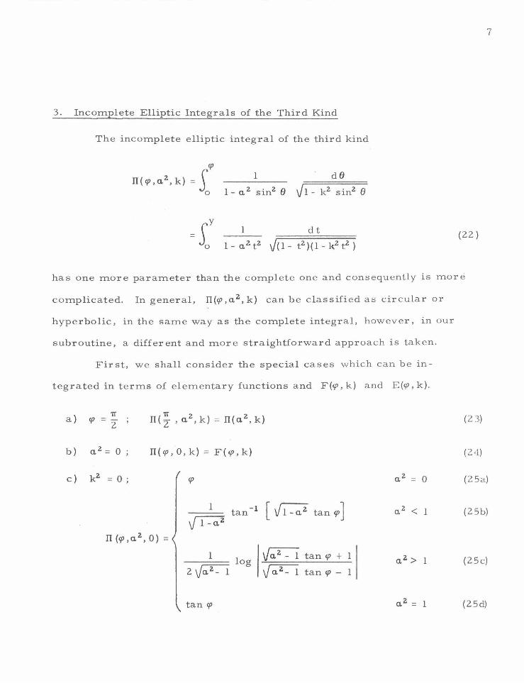
3. Incomplete Elliptic Integrals of the Third Kind
The incomplete elliptic integral of the third kind
cp
TI(cp,a.z, k) = s 0
1 dB
1 dt
l - a. 2 t 2 J (l - t 2 )( 1 - k 2 t 2 )
7
(22)
has one more parameter than the complete one and consequently is mor e
complicated. In general, I1 (cp, a. 2 , k) can be classified as circular or
hyperbolic, in the same way as the complete integral, however, in our
subroutine, a different and more straightforward approach is taken.
First, we shall consider the special cases which can be in-
tegrated in terms of elementary functions and F(cp, k) and E(cp, k).
a)
b)
c)
"iT cp -z-
a.2= 0
k2 = 0;
( "iT z )- 2 n 2 ,a. ,k -IT(a. ,k)
IT(cp,O,k) = F(cp,k)
-;:==1~ tan -l [ {1":;;2 tan cp] Jl-a.Z
ll(cp,a. 2 ,0) = l
2~
tan cp
log J a. 2 - 1 tan cp + 1
J a. 2 - 1 tan cp - 1
(2 3)
(24)
(25 a)
(25b)
(25c)
(25d)

d) k = 1;
II (cp ,a. 2 , 1) =
sincp + {- log [ 1 + s~ncp] 2 cos cp 1- s1ncp
-1- [log (tan cp + sec cp)
1- a.Z
lo 11 + a. s~n cp I] g 1 -0. Sln cp
1 [log (tan cp + sec cp)
1- a.Z
+ ~ tan -l ( J'la'ZT sin cp )]
Il(cp,1,k) =[k' 2 F(cp,k)- E(cp,k)
+tan cpJ1- k 2 sin2 cp ]kr-Z
f) I kz . ] = lE(cp, k) _ smcp cos cp k' -z
J1 - k 2 sin2 cp
The remaining values of a. 2, for 0 < k 2 < 1, and 0 < cp < rr/2
can be divided into three regions, with two series expansione [5]. In
the regions
the series expansion is
where
00
= \ b kzm L m ' m= 0
sin2 me dO
1 - a. z sin2 e
8
(26a)
(26b)
(26 c)
(27)
(28)
(29)

Hence
b
b - cp 0
= 0
b 2
1
~
1
2 Ja.2-
= 1
16a.4
and the recurr ence r elation is
1
tan - 1 [ J1 -a. 2 tan cp] a. 2 < 1 (30)
log Ja.2- 1 tan cp + 1
Ja.z- 1 tan cp - 1 a. 2 > l (31)
[ 3a. 2 sin cp cos cp + 6 b - 3 ( 2 + a. 2 ) cp] 0
9
2(m+l}a. 2 b +l= (2m+l+2ma. 2 }b +(l-2m)b 1-(-)m ( -i) sin2 m-lcpcoscp
m m m- m-1
In the region I a. 2 1 < 1 , k 2 < 1
a different series expansion is valid,
Both series can be derived very eas ily. Th e series in Eq. (29) is obtained
by expanding the quantity
(1-k' sin'B)-} o I (;;t) (-k')m sin'me
m =0
and the series in Eq . (32) , by the above expansion times the geometric
series expansion of 00
(1 -a. 2 sin2 e)- 1 = L (a. 2 sin2 e)j.
j = 0
Term by term integrations are th e n carrie d out for both expansions.
The regions of validity of th e two series, with their overlapping

region l > la. 2 i > k 2 are shown in Fig. 2.
~ OVERLAPPING REGION -
-I - kz 0 kz I az axis CXl
I CXl
Series given by Eq . (32)
-b. given by b. given by-Eq. (30) Eq . (31)
b. given by Eq . (30)
Series given by Eq . ( 29) t----- Series given by Eq . (29) ----
Figure 2
We have chosen to evaluate the integral in this common region by Eq. (29).
For values of ({) and k such that k 2 sin2 ({) is near one, both series ex-
pans ions for IT(({) ,a. 2 , k) converge slowly and henc e certain addition
formulae [5] ':'must be used to facilitate these calculations. These addi-
tion formulae are of the form
10
(33)
where
or
() = 2 tan -1 [ sin({) J1 -k2 sin2 f3 ± sin f3 J l-k2 sinz ({) ] cos (/) + cos f3
() = cos -1 [cos<p cos f3 + sin<p sinf3 J(l-k2 sin2 <p) (l-k2 sin2 f3) J . l -k2 sin2 <p sin2 f3
(34)
(35)
·'· .,. Some errors of sign for thes e formula e w e r e found in this r e fer e nce.

We now let
and
Q = a
Qb = ia. 2 _ 1 ~ (: 2 _ k2 )
Then for
sin(/' sinf3 sine Ja. 2(l-a. 2) (a. 2-k2) ]
sin2 e ±a. 2 sin(/' sinf3 cos e Jl-k2sin2 e
tanh -1 [--....:.s....::.i::....n_:_(/'_s _in_!_f3_s_i_n_e___:J_a._2_!(a._
2 _- _1 ~) ~(a.;::2=-=k:::::2===) ==::==e ] .
l-a. 2sin2 e±a. 2sinqJ sinf3 cose Vl-k2 sin2
-oo< a. 2< 0 Q = -Q a'
0 < a.2 < k2 Q = Qb;
k2 < a.2 < l Q = Q · a'
l<a. 2 <oo Q = Q b
In order to apply these formulae to our problem one must assign a value
to f3' choose a sign and then calculate a e from the given (/} and k.
The proper choic e of f3 and sign will produc e a e < qJ and hence th e
series for rr(e ,a. 2 , k) will converge with f ewer terms than the series for
Obviously the choice of f3 and th e sign is rather important. The
minimum e occurs when f3 = lT I 4 and th e lower sign is chosen. Making
this substitution and choosing Eq. (34) the more convenient form for e,
th e addition formulae can b e written as
II(qJ,a. 2,k) = rr{e,a. 2 ,k) + II(n"/4,a. 2,k) + Q
ll
(36)
( 37)
( 38)
{39)
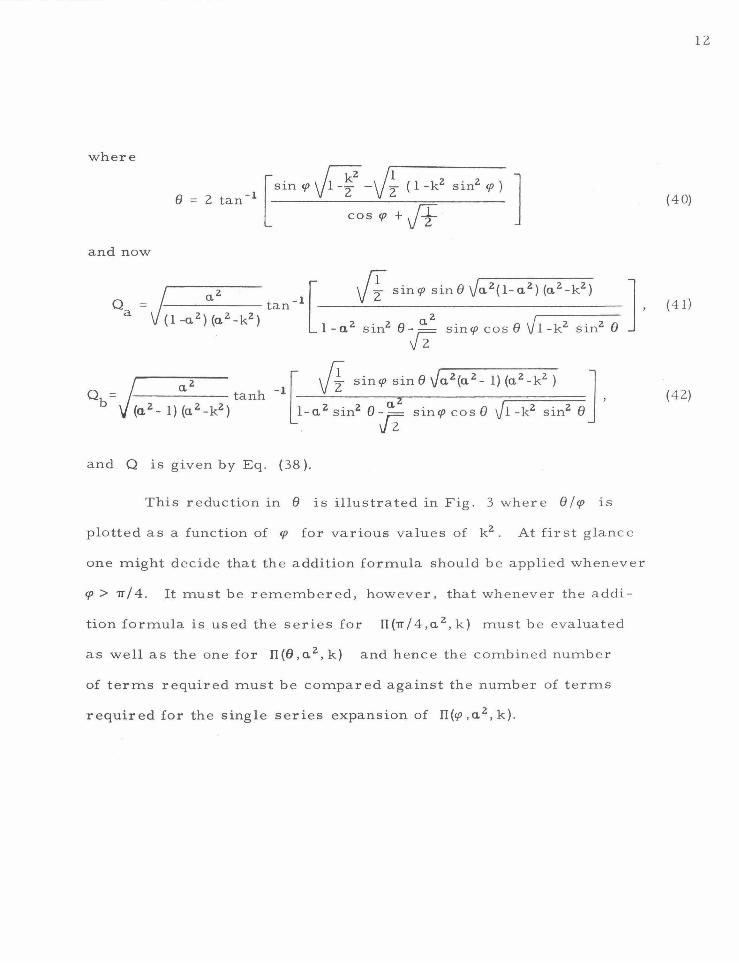
where
and now
Q = b
[
sin cp ~ -J~ ( 1 -k2
sin2
cp) ]
cos cp + ~
and Q is given by Eq. (38 ).
This reduction in f) is illustrated in Fig. 3 where 8/cp is
plotted as a function of cp for various values of k 2 . At first glance
one might decide that the addition formula should be applied whenever
cp > TT/4. It must be remembered, however, that whenever the addi-
tion formula is used the series for ll(TT/4 , a. 2 , k) must be evaluated
as well as the one for n(fJ,a. 2 , k) and hence the combined number
of terms required must be compared against the number of terms
required for the single series expansion of n(cp ,a. 2 , k) .
12
(40)
( 41)
(42)

13
1.4
1.2
1.0
0.8 0 .9
0.8
0.6
0.4
0.2
8 0 cp 10 20 30 60
cp, DEGREES
70 80 90
-0.2
-0.4
-0.6
-0.8
-1.0
-1.2
-I .4 L--------.1.....&----------------------------'
Figure 3 . Variation of 8 /cp with cp for several values of the modulus k 2.
8 is calculated by Eq. (34 ).

For values of k 2 very near one, the reduction in qJ is not
sufficient to as sure fast convergence, and therefore repeated applica-
tion of the addition formula can be carried out. Let () be the final n
value of 9 after the addition formula has been applied n times. Then
the integral can be expressed as follows:
where
so that,
Il(qJ,a. 2, k) = nll(1T/4,a. 2 , k) +II(() ,a. 2 , k) + Q
n
_ [sinqJ Jf- )"Iz: ( 1-k2
sin2
qJ)] () = 2 tan 1 ,
1 cos qJ +[f
() = z [
sin() Jl- kz - )!:... ( 1- k 2 sin2 () } ]
2 -1 1 2 2 1 ~n ,
cos () + !I 1 v 2
() = 2 tan -1 n- 1 V 1 - 2 2 n- 1 .
[
sin() V' - ji ( 1- k 2 sinz () ) ]
cos ()n-L +Ji n
+ + .
14
(43)
(44}
( 45)

and
~ =);a}- l~:nz- kz)
+ + .
1 [ ~ sinq> sin en Ja
2(a
2- 1) (a.
2-k
2) J l
+ tanh- If J 2 . 2 · ] -nz (sirf e + L sinq> cos e 1-k Sln en)
n 2 n
Again Q is given by Eq, (38 ).
Table I illustrates how well repeated application of the addition
formula works for the most difficult cases exp e cted to be encountered.
In this table values of e for n = 1, 2, 3, 4, 5 are shown for q> =- rr/2 n
and k 2 = 0 . 9990 and 0. 9999.
Table I Reduction of the Ar g ume nt
kz q> el e e3 e e 2 4 ~
0. 9990 rr/2 1.5392 1. 4820 1. 3518 1. 0499 0.4271
0. 9999 TT/2 1. 56 08 1. 5425 1. 5008 l. 4015 1 . 1664 ___j
Test runs were made with our program and the t o tal numbl' r o f
terms were recorded for cases when the addition formula was used and
when it was not used. We found that the least computer ti1n e r e sult e d
if we used the addition formula for values of q> and k such that
(46)
15

k sin cp> 0. 7 5. Furthermore, the addition formula is repeatedly used
until k sine < 0.75. In this way we were able to calculate II(cp,a. 2, k)
n
forallranges of a. 2 , la. 2 -k2 I>O . l,':<where O<cp<l.570 and
0< k 2 < 0.999 using less than a total of 25 terms.
The flow chart and a copy of the subroutine are given in Appen -
dix C.
-·. ,. The details of the r eg ion la. 2 - k 2 I:S 0.1 are given in Appendix C .
16

17
APPENDICES
Appendix A. Approximate functions for the complete elliptic integrals
of the first and second kind.
The complete elliptic integrals of the first and second kind, i.e. ,
K(k) (A. I)
TT I 2.
E(k) = s J,-l---k-2-sl-.n-2_8_ de 0
(A.2)
where 0 ~ k 2 < l, can be calculated by the approximate functions [ 3]
+ {b + b T} + b T} 2 + b T}3 + b T} 4 }log.!_ 0 1 2. 3 4 T}
(A. 3)
and
(A.4)
In these equations
and the coefficients as given in Ref. [3] are

a= 1.3862,9436,112 b = 0.5 0 0
a = 0 . 0966,6344,259 b = 0. 1249,8593,597 1 1
a = 0. 0359,0092,383 b = 0.0688,0248,576 z z
a = 0. 0374,2563,713 b = 0. 0332,8355,346 3 3
a = 0. 0145,1196,212 b = 0. 0044,1787,012 4 4
c = 0.4432,5141,463 d = 0. 2499,8368,310 1 1
c = 0. 0626, 0601' 220 d = 0. 0920,0180,037 2 2
c = 0. 0475,7383,546 d = 0.0406,9697,526 3 3
c = 0. 0173,6506,451 d = 0. 0052,6449,639 4 4
The error curves of these approximation functions are shown in
Fig. A-1.
1.0 X I 0- 8
- 1.0 X I 0- 8
Figure A -- 1. Error inK':' and E ,:, as a function of sin- 1k. This figure is given in Ref. [3], p 172.
18

19
The subroutines of these functions are not included since they are
quite straightforward.
Appendix B: The Evaluation of the Incomplete Elliptic Integrals of the
First and Second Kind.
The incomplete elliptic integrals of the first and second kind
F(rp, k)
are evaluated by two types of series and some special formulae for the
boundary condition cases. The reader may refer to Ref. 4 for detailed
discussion of these series expansions.
In the range 0 < j k sinrp I < tanh 1 = 0. 7615, 942 the series ex-
pansions are evaluated by the equations
F(rp,k) (2n}!
z2 n n! 2
and
00
E(rp' k) = -I (2n)!
n=O
~.qJ
k 2 n j sin2 n e d e 0
(B . la)
(B.l b)
(B.2a}
(B. 2b)
These formulae can be derived directly by the binomial expansion of the
integrands of F(rp, k) and E(rp, k) in Eqs. (B.l ). Though these series
are convergent for the entire range of qJ and k, their convergence is

slow when lk sinq> l >tanh 1. A second set of series therefore is used
to evaluate F(q>, k) and E(q>, k) in the range
tanh l < lk sinq>l < l.
These are presented in Ref. 4 and are
F(tp,k) = ~ K' log [ 4 ] + lkl J 1-~ log [1+ lkxl] • J1-kz~+ lkl ~ 1-kzxz ---z--
~ ~ z lkl Vr:(:-1--~--;-:),...,(:-1---k•'~.......,.)I f;_"n
1!;, (1-kz~)n I [ (2mt2)! J (k')zm-zn
n = 0 nt . m = n + 1 zZmtz (mt I ) ! Z
~ [ (Zn)! ] z
n~1 zznn!Z m(Zm-1)
where
x = sin q>
20
(B.3a)
(B.3b)

Our subroutine for F(cp, k) and E(cp, k) follows closely the one
suggested in Ref. 4, pages ll to 14. The flow chart and a copy of the
subroutine written in Fortran IV language for the IBM 7090 are given
in Appendix C.
The maximum number of terms required to yield six decimal
places in the neighborhood of k sin cp =tanh 1 is nineteen terms for
the first series method (Eqs. (B.2)), and fourteen terms for the sec
ond method (Eqs. (B. 3 )). It should also be pointed out that even though
Eqs. (B.3) are theoretically good in th e regions of k sin cp = 1, when
k 2 sin2 cp exceeds 0.99 the number of significant figures is reduced.
This loss in accuracy occurs becaus e the quantity 1- k 2 sin2 cp must
be evaluated.
A few words are also needed for the boundary condition cases:
Case 1: k 2 near 0
This presents no special problem since the first series (B.2)
will converge rapidly. We have arbitrarily considered k 2 < l 0-7
to be equal to zero and hence only the first terms of the series in
Eqs. (B.2) are required yielding
F(cp,O) = cp
and
E(cp,O)=cp
21

!T(a2,k) • Eq.(l2) where 8 • Eq.(l3) Return
.z < -k
where 8• Eq.(l I) f---k<a2<0 1100
D(a2,k) • Eq.(IO) ~
Return
O(k2,kl • Eq.(6) Return
M •1,3
8~·----- M • 2 __i_ la2 - k21 s 10-4
fl(a2,k) • Eq.(l4) where 8 • Eq.( 15) Return
nla2,k) • Eq.(l6) where 8 • Eq.(l7) Return
[J(a2 ,k) • Eq.(20) where 8 • E q.(21l Return
M • I
[J(a2,k) • Eq.(5)
Return
M=2
M=3
O(a2,k) = Eq.(l8) where 8 • Eq.(l9)
Return
nlf>,a2,kl • Eq.( 32)
Return
Addition formula Eq.(43) where
{
Eq.(46), Q•
-Eq.(45),
until ksin8n <0.75,
then ITI8n ,a2,kl • Eq.(32) Return
ENTER
8--i O(O,i,kl=O Test 4> 4>•0---• 10 '------J . Return
<i>JtO
lt-a2 l ~0.1 and --...-(
>0.9999 k2 s 0.9
)l-a2(<0.1 and (1-asin<l>l<!:I0-4
or k
2 > 0.9 and k sin 4> :S 0.9999
8
?-----1---- + • f 0< +< f ----..1. 20
; <0 or
•Pf
n{f>,O,k) • Flr;,kl
Return
filf>,l,k) = Eq.(27)
Return
k sin; <0.75
~ lazl< kz ---<
k sin;< 0.75
>--- a2> I --e( k sin;> 0.75
Addition formula Eq.(43) where.
{
Eq.(46), a2 > 0 Q•
-Eq.(45), a2 <0
until k sin8n < 0.75,
then D (S,,a2,kl• Eq.(29).
Return
k2 < la21 < I or .. 2 <-I
ksln; <0.75
k sin;> 0.75
DC<~o,a2,kl • Eq.(29)
where b. • Eq.(30)
Return
D!-;, .. 2,1) = Eq.(26c)
Return
D(f>,a2,kl • Eq.(29l
whefe b.• Eq.(31)
Return
Addition formula Eq.(43)
where Q • Eq.(46)
until k sin 8n < 0.75,
then 0(8,.,ca2,k) • Eq,(29).
Return
Figure C-1. The flow chart of Subroutine PIX for calculation of the complete or incomplete elliptic integral of the third kir.d. The circled numbers in the flow chart refer to statement numbers in the pJgram listing in Fig. C -2.
0.9999 < k2 s I
Il(r;,I,Ol • ton f>
Return
R(.,c2,kl • Eq.(25el Return
ll(f>,l,l) • Eq.(26a)
Return

F(cp, k) and E(cp, k) have the following series expansions [5]
1n powers of k 12
F(cp, k) = k ,zm p (cp) zm
m = O
where
l+sinm = log ___ '~";__ coscp
p (cp) 2
1 1
1 + sin <p --z og cos<p
p (cp) = - 1-[sinzm-l cp sec2 mcp+(l -2m)p (cp)] zm zm zm- z
and
00
E(cp, k) = I(l)k'zm dzm (cp)
m= 0
where
d (cp) = sincp 0
. 1 + sincp d (cp) = - smcp +log ___ ;__ oil cos <P
d4
(cp) = ·H sin3 <P sec2 <p + 3 sincp - 3 log 1 ~:;~<P]
d ( ) 1 [sinzm-l <p sec2 (m-l)m + (l-2m)d ( ) (cp)]
zm <P = 2(m-l) r z m-1
with m=fl.
22
(B.4a)
(B .4b)

Again we have arbitrarily considered 10-7
our criterion for
zero. That is we have taken lk' 2 l~ 10- 7 to be k' 2 = 0 or jl.O-k2 j~ 10-7
to be the same as k 2 = 1. 0 so that F and E are r epr es en ted by their
first terms in Eqs. (B.4) giving
F(<p, 1) = log (tan <p + seccp)
and
E(<p, 1) = sin cp
The flow chart and Fortran IV program are given in Appendix C.
23

Appendix C . The most frequently used symbols in the subroutine list-
ings in Figs. C-2 and C-4 have the following definitions:
AS
XK
SK
PK
PHI
THE
K
Ec
F
E
PI
TOL
M
I a)
a.~
k
kz
k'
cp
()
-·--·-K
-·--·-E
F(cp,k)
E(cp,k)
Il(cp,a. 2 ,k) or I1 (a. z' k)
Allowable error
Accuracy or error indicator - (output)
M = l, less than four figure accuracy or error return due to non-convergence, overflow or illegal parameter in argument
M= 2, six figure accuracy
M = 3, four to six figure accuracy
Indicator in subroutine PIX - (output)
I= 0, () , F, and E were not calculated
I= l, 0, F(O,k') and E(O,k') were calculated
I= 2, (), F(O, k) and E(O , k) were calculated
24

b) Indicator in subroutine ELLI - (input)
I= l, both F and E to be calculated
I=2, calculate E only
I= 3, calculate F only
Figures C-I and C-2 are the flow chart and Fortran IV listing for
the subroutine which calculates IT(a. 2 ,k) or IT(q~,a. 2 ,k) the complete or
incomplete elliptic integral of the third kind. The circled numbers in
Fig. C -1 refer to statement numbers in the program listing given in
Fig. C-2.
Six figure accuracy is guaranteed except when II- a. 2 I< O.I or
k 2 > 0 . 9 and at least four figure accuracy is guaranteed when II- a. sinq~l
~ 0. 0001 and k sinq~~ 0. 9999. The accuracy indicator M is set as des
cribed above and a message is printed whenever the accuracy is less
than six figures.
If ksinq~ isgreaterthan0.75or ql=tr/2 themethodsoutlinedin
the text cannot calculate IT(a. 2 ,k) or IT(q~,a. 2 ,k) to six figures when
la. 2- k 2 1 ~ O.I or to four figures when la. 2 - k 2 1 ~ 0. 000 I, because accuracy
is lost in calculating the quantity a. 2 - k 2 . Therefore, our program trans
fers control to statement number lOI using Eq. (32), without the addi
tion formulae for both integrals whenever Ia. 2 - k 2 I is less than or
equal to 0. 1 and M = 2 (six figure accuracy); thus the quantity a. 2 - k 2
need not be evaluated. When la. 2 - k 2 ~~ 0. 0001 and no more than four
figure accuracy is required (M =I or M = 3), a. 2 is considered to be
the same as k 2 so that
II (q~, a. 2 , k) = II (q~, k 2 , k)
25

or
IT(n 2 , k) = IT(k2 , k).
The remaining deviation from the text is the case when cp = Tr/2, M = 3
and 0. 000 l < \n2.- k 2 j < 0.1 . For this case better accuracy is obtained if
IT(n 2, k) is calculated as a special case of th e incompl e t e integral.
The flow chart and Fortran IV listing for the subroutine which
calculates the incomple te elliptic integrals of the first and second kind
are given in Figs. C-3 and C-4 respectively. As above , the circled
numbers in the flow chart correspond to statement numbers in the pro
gram listing.
26

Fig
ure
C-2
. T
he F
ort
ran
IV
lis
tin
g o
f S
ub
rou
tin
e P
IX.
SUB
RO
UT
INE
P
IX(
PH
I ,A
S,X
K,
TO
L,M
1 P
I ,K
,EC
, I,
TH
E ,F
,El
l F
OR
MA
TI1
9H
PHI
NE'
G
OR
GT
Pl/
21
2
FOR
MA
T I
7H
K
G T
l)
3 F
OR
MA
T1
30
H
PI
AT
LE
AS
T
4 F
IGU
RE
A
CC
UR
AC
Y)
4 FO
RM
AT
! IS
H
OV
ER
FLO
W
IN
Pll
5
FOR
MA
T 11
7H
P
I N
OT
CO
NV
ER
GE
D I
6
FO
RM
AT
I20
H
PI
NE
AR
S
ING
UL
AR
ITY
) 1
00
7
FO
RM
AT
I22H
A
S O
R SK
=ON
E1
PIC
=IN
FI
RE
AL
K,
N
DIM
EN
SIO
N
81
10
11
T
AL
=O
. p
1 f:
.:Q
. Q
::z:
Q.
NN
=l
TH
E=
O.
pI
:zQ
.
N:O
. I
=0
E
C=
l..
K=
O.
F=
O.
E=
O.
CA
LL
O
VE
RF
LI
L1
IFIA
BS
IPH
il.L
E •
• O
OO
OO
Oll
GO
TO
10
S
K=
XK
•XK
S
P=
SIN
IPH
I I
A=
SQ
RT
IAB
SIA
S)I
A
SP
=A
•SP
IF
IAS
.LT
.O.t
A
SP
=-A
SP
IF
!AB
S!l
.O-A
SI.
GE
•• l
.AN
O.S
K.L
E •
• 9
1 G
O
TO
8 IF
IAB
SI
l.O
-A.S
Pl.
LT
••
OO
Ol
.O
R.X
K•S
P.
GT
•• 9
99
9l
GO
TO
7
WR
ITE
I b
o 3
1 fo
1:3
GO
TO
9
7 W
RIT
EI6
,61
11
=1
GO
TO
9
8 11
=2
9 IF
I.O
OO
OO
Ol.
LT
.PH
I.A
NO
.PH
I.L
T.l
.57
07
96
21
GO
TO
2
0
lFIA
BS
IPH
I-1
.57
07
96
31
.LE
....
OO
OO
OO
l)
GO
TO
1
00
0
WR
ITE
16
r 11
M
= 1
RE
TU
RN
1
0 P
I =
0.
M=
2 R
ET
UR
N
20
C
P=
CO
SIP
HI
I S
PS
=S
P•S
P
IFL
OO
OO
OO
L.L
T.S
K.A
NO
.SK
.LE
... 9
99
91
G
O
TO
30
IF
ISK
.LE
••
OO
OO
OO
ll
GO
TO
4
0
IFIS
K.L
T.1
.0
00
00
0ll
G
O
TO
50
W
RIT
E
16
,21
M
=1
RE
TU
RN
4
0
IFIA
BS
IAS
I.L
E..
OO
OO
OO
ll
GO
TO
4
3
IFIA
BS
IAS
-1.Q
I.L
T ..
. 0
00
11
GO
T
O
41
IF
IAS
.GT
.L.O
I G
O
TO
42
X
=S
CR
Til
.O-A
SI
PI=
AT
AN
IX•S
P/C
PI/
X
RE
TU
RN
4
1
PI
=S
P/C
P
RE
TU
RN
4
2
X=
SQ
RT
IAS
-1.0
1
PI
=.5
/X•A
LO
GI
AB
S I
II X
•SP
/CP
I+l.
1/1
I X
•SP
/CP
J-1
.o
I I
I R
ET
UR
N
43
P
I=P
HI
M=
2 R
ET
UR
N
50
lF
IAB
SIA
S-l
.O
).L
T.
.OO
Oll
G
O
TO
5
2
IF!A
S.L
T .
0.1
G
O
TO
53
P
I =
I A
LO
G I
( S
P+
t.O
1/C
PI-
0.
S•h
AL
OG
lA
BS
( l
l.O
+A
SP
l/ (
1.0
-AS
P l
J II/
lll.
O-A
Sl
RE
TU
RN
5
2
PI=
.S•I
SP
/IC
P•C
PI+
.S•A
LO
Gtl
l.O
+S
PI/
11
.0-S
Pll
l R
E 1
UI(
N
53
P
i=IA
LO
G(I
SP
+t.
OI/
CP
ltA
•AT
AN
I-A
SP
J 1
/11
.0-A
SI
~E T
UR
\1
30
IF
IAB
SIA
S)
.L
( ••
OO
OO
OO
LI
GO
TO
3
1
IFIA
BS
IAS
-1.0
l.L
T •• O
OO
ll
GO
TO
3
2
IFIA
BS
IAS
-SK
I.L
f ••
OO
OO
OO
ll
GO
TU
3
3
IFIA
BS
IAS
-SK
I.L
E •
• 0
00
1l
GO
TO
(3
3,1
01
,33
1,M
IF
IAB
S(A
S-S
KJ.
LE
.O ..
ll
GO
TO
1
35
r10
1,3
51
,M
GO
TO
3
5
3l
CA
LL
E
llli
PH
I,X
K,F
,E,J
,L,T
Oll
P
I :~
:f
RE
TU
RN
3
2
CA
LL
E
lll(
PH
J,
XK
,F,E
,t,L
,TO
L)
PI
=I
I 1
.u
-SK
I•F
-E+
SP
/CP
•SQ
RT
I 1
.0-S
K•
SP
S 1
1/1
1 .0
-SK
I R
ETU
RN
3
3
CA
LL
E
LL
IIP
HI,
XK
,F
,Er2
rl.T
Oll
P
I =
I E
-SK
•S
P•C
P/S
QR
T 1
1. 0
-SK
•SP
S I
I I
I 1
.0
-SK
I R
ET
UR
N
35
IF
IAB
SIA
S).
LT
.SK
I G
O
TO
IOU
IF
ISK
.LT
.AtJ
SIA
Sl.
AN
O.A
BS
IAS
l.L
T.1
.01
G
O
TO
20
0
IFIA
S.
GT
.l.
OI
GO
TO
3
00
2
00
1
F(X
K•S
P.L
T •
• 7
51
G
O
TO
25
2
20
1 TH
E:2
. 0
• A
T A
Nt
( SQ
R T
I 1
.0-. 5
•SK
I•S
P-.
70
71
06
78
•SU
RT
I 1
.0-S
K•S
PS
II
I 1
ICP
+.7
07
10
67
81
1
ST
:::S
IN
I TH
E I
CT
=C
OS
I TH
E I
ST
S=
ST
•ST
Q
:SQ
R T
I A
S/ Ill. 0
-A
S 1
•1 A
S-S
KI
II •
1'\T
AN
I+
. 7
07
10
6 7
B •S
P•
ST •
SQ
RT
I A
S•
( l
.0
-1
AS
I •
I A
S-S
KI
1/1
l.
0-
AS
• S
TS
-. 7
07
10
6 7
8•A
S•S
P•C
T •S
OR
T I
1.-
SK•S
TS
I J
I +Q
P
HI=
-TH
E
SP
=S
T
CP
=C
T
SP
S=
SP
•S
P
TA
L=
TA
L+
I.O
lF
IX
K•S
P.G
T..7
51
GO
TO
2
01
N
N=
2 G
O
TO
2
52
2
10
P
IT=
PI
Tl =
N
NN
=3
PH
I=. 7
85
39
81
6
SP
= ..
70
71
06
78
C
P=
. 7
07
10
67
8
SP
S=
. 5
GO
T
O
25
2
21
1
IFIA
S.L
T.O
.I
GO
TO
2
12
P
I=T
Al
•P
l+P
ITtQ
R
ET
UR
N
21
2
Pl=
lftl
•PI+
PIT
-U
RE
TU
RN
2
52
S
AS
=S
QR
Til
.O-A
Sl
BO
:A T
AN
t SA
S•S
P /C
P 1
/SA
S
25
1
Bl
11=
.5
•(8
0-P
Hli
/AS
S
C:S
P•C
P
TK=
SK
•SK
6
t 21
= .
06
25
•13
. O
ttA
S•S
C+
6.
O•B
O-
I 6.0
+3
.0•A
S J
•PH
II I
I A
S•A
S I
PI
:z:B
O+
Bil
lttS
K+
BI2
J•T
K
OM
=-S
C
EM
:-.
5 J:.
5•
(PH
I-S
Cl
DO
2
60
J=
Z,
LOO
N
=J
TN
:2•J
SC
:SC
•SP
S
OM
:OM
•I f>
l-1
. 5
I •S
PS
/ IN
-1.
01
E
M=E
M•IN
-1
.51
/N
T
=(
{ T
N-1
.0l
•T-S
CI/
TN
0
1 J•ll =
II T
N+
l.O
tTN
•AS
) •
B I
J I tl
1. 0
-T
NJ
•B I
J-1
1-D
M-E
M•T
II
I A
S•I
TN
+2
.0
1 I
TK
=S
K•T
K
TE
RM
=B
IJ+
11
•TK
P
I=P
I+T
ER
M
lFIA
BS
I IE
.lM
).L
E.T
Oll
G
O
TO
15
0l,
21
0,
2ll
t31
0,
31
li,N
N
26
0
CU
NT
IN
UE
2
61
\oiR
ITE
(6,
'il
M=
1 ~E T
UR
N
10
0
IFIX
K•S
P.
GT
..7
51
G
O
TO
10
2
10
1
SC
=S
P•C
P A
K:-
SK
/1\S
T
=."
J•I
Pii
i-S
CI
A T
:AS

Fig
ure
C-2
co
nti
nu
ed
C=
-.5
•AK
C
M:l
.Q+
C
Pl=
CM
•AT
•T
DO
1
10
M
M=
2,2
00
N
=H
M
TN
=2
•MM
S
C=
SC
•SP
S
T=
(l T
N-l
.Ol•
T-S
CI/
TN
A
T=
AT
•AS
C
=C
• I 0
. 5
-N I•A
K/N
C
H:C
M+
C
SM
=C
H•A
T•T
P
J:P
J+S
H
IFIA
BS
tSM
I(P
J+P
HI)
).L
E.T
OL
I G
O
TO
10
3
IFIA
BS
IAT
I.G
T.L
O
E-3
01
G
O
TO
11
0
Af:
AT
•L.O
E
30
C
=C
•l.O
E
-30
C
M=
CH
•l.O
E
-30
1
10
C
ON
TIN
UE
G
O
TO
26
1
10
3
PI=
PI+
PH
I GO
TO
15
0lt
l2lt
l22
1,N
N
10
2
TH
E=
Z. O
•AT
AN I
t SQ
R T
I 1.0
-.
5•
SK l
• S
P-.
70
7L
06
7B
•SC
RT
II.
0-S
K•S
PS
I II
1 IC
P+
. 7
07
10
67
81
I
ST
=S
JNIT
HE
I C
T=
CO
SIT
HE
I S
TS
=S
hS
T
JF
IAS
.LT
.O.I
G
O
TO
10
5 Y
=
+. 7
07
10
67
8•
SP
•ST
•SQ
RT
lA
S•
I AS
-1
.01
• I A
S-S
K I
I/
l 1
1. 0
-AS
•S
TS
-. 7
07
l06
78
•S
P•C
T•
SQR
T I
1. 0
-SK
•S T
S I •
AS
I T
Y=
.5•
AL
OG
IAB
SI
t l.O
+Y
l/1
1.0
-YI
I I
Q=
SQ
RT
IAS
/1 I
AS
-l.O
l•IA
S-S
KII
l•T
Y+
Q
10
4
PH
I=T
HE
S
P=
S T
C
P•C
T
SP
S•S
TS
T
Al=
T A
l +
1.
0 IF
IXK
•SP
.GT
••
75
}
GO
TO
1
02
N
N=
2 G
O
TO
10
1
10
5
Q=
-SQ
R T
I A
S/I
I 1
.0-A
Sl •I
AS
-SK
I I
l•A
TA
N!.
70
7l0
67
8•
SP
•S
T•S
OR
T I A
S•Il.
0-
1 A
Sl•
IAS
-SK
II/1
1.0
-AS
•ST
S-.
70
71
06
78
•AS
•SP
•CT
•SO
RT
I1.-
SK
•ST
Sll
l+O
G
O
TO
10
4
12
1
PIT
=P
I N
N=
3 P
HI=
. 7
85
39
81
6
SP
=.
70
71
06
78
C
P=
.70
71
06
78
S
PS
=.5
G
O
TO
10
1
12
2
PI=
TA
L•P
l+P
IT+
Q
RE
TU
RN
3
00
IF
IXK
•SP
.GT
..7
5l
GO
TO
3
05
3
02
S
AO
=S
OR
TIA
S-1
.0
1
XX
=S
AO
•SP
/C
P
80
=.
5/S
AD
•AL
OG
lA
BS
II
XX
+ 1
.01
/1 X
X-1
.01
I I
GO
TO
2
51
3
05
T
HE
=2
.0•A
T A
N I
I S
OR
T 1
1. 0
-.
5•
SK I
•S
P-
. 7
07
l06
78
•SQ
R T
11
. 0
-SK
•S
PS
II/
1 IC
P+
.70
71
06
78
1 I
S
T=
S I
NI
TH
E I
C
T=
CO
SI
IHE
I
ST
S=
ST
•ST
Y
=+
.70
71
06
78
•SP
•ST
•S0
RT
lA
S•
IAS
-1.
01
•I
AS
-SK
I J/
1 1
1. 0
-AS
• S
TS
-. 7
07
10
67
8•
SP
•C
T•S
CR
T 1
1. 0
-SK
•S
TS
J •A
S l
TY
=.
5•A
LO
GI
AS
S I
ll.
O+
YI/
11
.0-Y
J J
I
Q=
SQ
R T
I A
S/I
I A
S-1
.0 I
•IA
S-S
KI
li•T
Y+
Q
PH
I=T
HE
S
P=
S T
C
P=
CT
S
PS
=S
TS
T
AL
=T
AL
+1
.0
JFIX
K•S
P.G
T..
75
l G
O
TO
30
5
NN
=4
GO
TO
3
02
3
10
P
I T
=P
l N
N=
5 P
HI=
.78
53
98
16
S
P=
.70
71
06
78
CP
=.7
07
10
67
8
SP S
=.
5 GO
TO
3
02
3
11
P
l=T
AL
•PI+
PIT
+Q
5
01
C
AL
l O
VE
RF
UL
l IF
IL.E
Q.2
1 R
ETU
RN
W
RIT
EI6
,41
M
= 1
RE
TU
RN
1
00
0
IF I
AB
SIA
S-1
.0
).L
E •
• 0
00
00
01
. O
R.A
BS
I S
t<.-
1.0
I.L
E •
• 0
00
00
01
1
GO
TO
1
05
0 IF
I.
OO
OO
OO
l.L
T .S
K.A
NO
.SK
.LT
•• 9
99
99
99
0)
GO
TO
1
02
5
JFIS
K.L
E •
• O
OO
OO
Oll
G
O
TO
10
40
1
00
6
WR
ITE
(6,2
J H
= 1
RE
TU
RN
1
05
0
WR
ITE
16
, 1
00
71
M
•l
RE
TU
RN
1
04
0
IFIA
S.L
T •
• 9
99
99
99
01
G
O
TO
10
41
P
I =
0.
H=
2 R
ET
UR
N
10
41
P
I=
1.
57
07
96
3/S
QR
Til
.O-A
SJ
RE
TU
RN
1
02
5
PK
:SQ
RT
I 1
.0-S
KI
CA
ll
EL
IPT
IXK
,K,E
C,l
) IF
IAB
SIA
SI.
LE
••
OO
OO
OO
II
GO
TO
1
03
1 IF
IAR
SIA
BS
tAS
I-X
KI.
LE
•• O
OO
OO
Oll
G
O
TO
1
03
2
IFIA
S.L
T.
O.l
G
O
TO
11
00
lF
IA!J
SIA
S-S
KI.
LE
••
OO
OO
OO
ll
GO
TO
1
03
3
SP
S=
l.O
C
P=
O.
IFIA
BS
IAS
-SK
l.L
E •
• O
OO
ll
GO
TO
1
10
33
,10
1,1
03
3)
1/'
\
IFIA
BS
IAS
-SK
J.L
E.0
.11
G
O
TO
t10
26
,10
1,3
5l,
1'1
1
02
6
IF(A
S.G
T.S
K.
AN
O.A
S.L
E •
• 9
99
9)
GO
TO
12
00
IF
IAS
.LT
.SK
.AN
O.
AS
.G
T •
• 0
00
00
01
l G
O
TO
13
00
TH
E=
AS
IN
I S
QR
fi1
.0/A
S J
I
CA
ll
EL
LII
TH
E,X
K,F
,f
,1,L
,TO
LI
PI
=IE
C•
F-K
•E
l •
SOR
T lA
S/{
IA
S-I
.OI•
{A
S-S
KII
I 1
=2
R
ET
UR
N
10
31
P
I=K
R
ETU
RN
1
03
2
PI
=0
.2
5•1
3.1
41
59
26
5+
2.0
•11
.0
-AS
I•
KI/
11
.0-A
SI
RE
TU
RN
1
03
3
PI=
E
C/1
1.0
-SK
I R
ET
UR
N
11
00
X
XK
=-X
K
IFtA
S.L
T.X
XK
I G
O
TO
11
02
T
HE
=A
SI
NI
SQR
Tl
AS
/IA
S-S
Kll
l C
AL
L
EL
LII
TH
E,P
K,F
,E,l
,l,T
OL
I P
I=
SK
•K/1
SK
-AS
l-A
S•
( EC
•F+
K•
I E
-F J
1/S
QR
T I
AS
• (
1.0
-AS
I•{
AS
-SK
II
J::1
R
ET
UR
N
11
02
T
HE
=A
SIN
I1.0
/SQ
R1
11
.0-A
SII
C
AL
L
EL
LJtT
HE
,PK
,F,E
,I,L
,TO
U
PI:
: K
/1 1
.0-A
S I
+A
S•
I E
C•F
+K
• I E
-F 1
-1.
57
07
96
3 I
I l
SQ
RT
IAS
•Il
.O-A
SI
•I
AS
-SK
ll
I= l
RE
TU
RN
1
20
0
IFIA
S.
GT
.XK
I G
O
TO
12
03
IH
E::
AS
IN
I S
QR
T I
I A
S-S
KI/
I A
S•
( 1
.0-S
KI
l II
C
AL
L
EL
LII
TH
E,P
K,F
,E,l
,L,T
OL
I P
I=
IEC
•F+
K•I
E-F
II•S
OR
TIA
S/I
IAS
-SK
I•Il
.O-A
SII
l I=
l R
ET
UR
N
12
03
T
HE
=A
SIN
ISO
RT
IIl.
O-A
SI/
11
.0-S
KII
I C
AL
L
EL
LJI
TH
E,P
K,F
1E
,l,L
,TU
LI
PI=
K
+l 1
.5 7
07
q6
3-
I E
C•F
+K
• IE
-F I
II
•S
OR
T I
AS
/I I
AS
-SK
l•t
1.0
-AS
I II
l =
I R
f TU
RN
1
30
0
TH
E=
AS
INIS
OR
TIA
S/S
KII
C
AL
L
EL
LII
TH
E,X
K,F
,E,l
1L
,TO
L)
PI=
K
+l
K•
E-E
C•F
I•
SQ
RH
AS
/1 I
1.0
-AS
I•I
SK
-AS
I I
I 1
=2
R
ET
UR
N
END

For Figures C -3 and C -4 the c:aptionu Bhould be interchanged.

Figure C-3. The flow chart of Subroutine ELLI for calculation of the incomplete elliptic integrals of the first and second kinds. The circled numbers in the flow chart refer to statement numbers in the program listing in Fig. C-4.
SU BROUTINE ElL I I PHI, XK,F,E,l ,M, TOll REAL N CALL OVERFLtMI F•O. f:::Q. SK=XK•XK IF I .QOO OOO l.l T .SK .. ANO.SK.LT •• 999999901 GO TO 25 IFISK.L E •• OOOOOOl) GO TO 20 lffABSCKK-l.OJ.LE •• OOOOOO ll GO TO 23
1~ WRITEI6,31 3 FORMAT 17H K GT 11
M•1 RETURN
20 E•PH I F=PHI M•2 RETURN
23 SP,SJN(PHI I E=SP H=2 JFCI.EQ.21 RETURN F"'AlOGI SP/ t COS I PHI I I +1. 0 / I COS I PHI I I)
10 CALL OVERFUMI JFIH.ECI.ll WRITEI6 1 41
4 FORMATI17H OVERFLOW IN ELLII RETURN
25 IF C. OOOOOOt.l T . PHI .AND. PHI.l T .1. 5707960 l JFIAB S IPHli.LE •• OOOOOO ll GO TO 41 IFIABSIPHJ-1.57079631.LE •• 0000003) GO TO
40 WRITE (6,51 5 FORMATI23H NEG PHI OR PHI GT Pl/21
M• 1 RETURN
41 fzQ. f:.:Q.
M•2 RETURN
44 CALL ELIPTIXK,F,E 1 MI RETURN
46 SP:SJNIPHI I AKP=XK•SP IFIAKP.GT..76l 59421 GO TO 45
43 SK=XK•XK CEz-.5•SK CF::o:-CE SPS=SP•SP CP.-COS I PHI I SC f:a::SP• CP f:::.5•1 PHI-SCTI E"'CE•T f:::Cf•T 00 64 J :o:2,200 N:::J TN--Z.O•N SCJ:a::SCT•SPS T= II TN-1.0 I •T-SCT 1/TN A=-SK/N CFaCf•l .5-Nl•A CEzCE•Il.5-Nl•A TCE =CE •T EzE+TCE TCF •CF•T F=-f+TCF GO TO 162,61,621, I
62 IF lABS CTCF I. LE. TOL I GO TO 65 GO TO 64
61 IF I ABSI TCE I .LE. TOLl GO TO 66 64 CONTINUE
M•1
GO TO
44
46
WRITE16r61 6 FORMATI19H ELLB NOT CONVERGED)
RETURN 65 f:zPHI+f bb E=PH I +E
GO TO 10 45 A=XK •CO SIPHI I
82-"' 1. 0-AKP •AKP IFI82. GE •• 05 1 GO TO 48 1FIB2.LT •• 00051 GO TO 47 WRIT E I b, l I
1 FORMATI32H F AND EAT LEAST 4 FIG.ACCURACYI M•J UO TO 49
47 WRITEI 6,2 l 2 FORMAT I 34H F AND E LESS THAN 4 FIG. ACCURACY I
M•l
48 49
90
91 200
GO 10 49 M•2 8-.oSQRTI!i21 ABL•ALOGI4.0/IA+81 I AOB=A/8 PKS:a::l.O-XK•XK XI • . 5 XJz . 25•PKS XL =1. 0 AB=A•fl XM:-AB•PKS•.I40625 XN=-AB•PKS•. 1875 S 1 ,.XM-XJ•Xl S2=XN- . 25 •PK S SJzXJ 54= . 75•XJ 00 200 J=2 t 100 N• J TN •2 •J C1 :TN-1.0 C2zC1/TN C3=f TN+1. 0 1/I TN+ 2 . 0 l C4=C3•PKS Aa•A6•82 CN• AB•XI/TN C02A=C2•PKS•XJ C02tl=PKS•XJ/I TN• TN I XJzC2•XI XJzC3•C4•XJ XL=XL+1.0/IN•Cll XMz I XM-AB•X 1/ TN l •C l •C4 XN: I XN-CN I•C4•C 2 Ol ::o: XM-XJ•XL 02 =XN-C02A • XL +(028 Sl:Sl+Ol S2,..S2+02 SJ::o:SJ+XJ S4:S4+C3•XJ GO 10 190,91,90) " IF IABSIDll .LE. lOU GO ro 200 IF IABSI0 2 I .LE. TOLl CONTINUE M• 1 WRITE 16 1 61 RETURN
GO
GO
10 210
TO 2ll
210 F= I 1.0+ 53 1 •ABL+AOB•ALOG I. 5+ .5•AKPI +51 IF(I. EQ.3 1 RETURN
2 11 f:: I. 5 + S4l •PK S•ABL+ 1. 0-AOB•Il.O-AKP l + 52 RETURN END

E (
¢, k
) =
sin
¢
I F
(¢
,k)=
lo
g(t
an
¢)+
CO
S<
/! R
etu
rn
E (¢
, k)
= 0
F (¢
,k)
= 0
Re
turn
F(¢
,k)
= E
q.(
B.2
a)
E (
¢,k
) =
Eq
.(B
.2a
)
Re
turn
Fig
ure
C-4
.
EN
TE
R
E(¢
,k)
= E
F(¢
,k)=
K
Re
turn
E(¢
,k)=
¢
F (¢
, k)
= ¢
Re
turn
F (
¢, k
) =
Eq
. (B
. 3a
)
E (
¢, k
) =
E q
. ( B
. 3 a
)
Re
turn
Th
e F
ort
ran
IV
lis
tin
g o
f S
ub
rou
tin
e E
LL
I.

REFERENCES
1. Selfridge, R. G. , and Maxfield, J. E. , "A Table of the Incomplete Elliptic Integral of the Third Kind", Dover, 1958.
2. Belyakov, V. M., Kravtsova, R. N., and Rappoport, M. G. "Tables of Elliptic Integrals", Vol. 1, Academy NAUK SSSR, Moscow, 1962.
3. Hastings, Jr., Cecil, "Approximations for Digital Computer", Princeton University Press, 1955.
4. DiDonato, A. R., and Hershey, A. V., "New Formulae for Computing Incomplete Elliptic Integrals of the First and Second Kind", Computation and Exterior Ballistics Laboratory, U. S. Naval Proving Ground, Dahlgren, Virginia, NAVORD Report No. 5906, January 1959.
5. Byrd, P. F. , and Friedman, M. D. , "Handbook of Elliptic Integrals for Engineers and Physicists", Springer-Verlag, Berlin, 1954.
27

DISTRIBUTION LIST FOR UNCLASSIFIED TECHNICAL REP O RTS
ISSUED UNDER CONTRACT Nonr -220(43)
(Single copies unless otherwise specified)
Chief of Naval Research Department of the Navy Washington 25, D.C. Attn: Codes 438 ( 3)
461 463 466
Commanding Officer Office of Naval Research Branch Office 495 Summer Street Boston l 0, Massachusetts
Commanding Officer Office of Naval Research Branch Office 207 West 24th Street New York 11, New York.
Commanding Officer Office of Naval Research Branch Office 1 0 30 East Green Street Pasadena, California
Commanding Officer Office of Naval Research Branch Office 1 000 Geary Street San Francisco 9, California
Commanding Officer Office of Naval Research Branch Office Box 39, Navy No. 100 Fleet Post Office New York, New York (25)
Director Naval Research Laboratory Washington 25, D. C. Attn: Code 2027 (6)
Chief, Bureau of Naval Weapons Department of the Navy Washington 25, D. C. Attn: Codes RUAW-r
Commander
RRRE RAAD RAAD-222 DIS-42
U. S. Naval Ordnance Test Station China Lake, California Attn: Code 753
Chief, Bureau of Ships Department of the Navy Washington 25, D. C. Attn : Codes 310
312 335 420 421 440 442 449
Chief, Bureau of Yards and Docks Department of the Navy Washington 25, D. C. Attn: Code D-400
Commanding Officer and Director David Taylor Model Basin Washington 7, D. C. Attn: Codes l 08
142 500 513 520 525 526 526A 530 533 580 585 589 591 591A 700
Commander U.S. Naval Ordnance Test Station Pasadena Annex 3202 E. Foothill Blvd. Pasadena 8, California Attn: Code P-508
Commander Planning Department Portsmouth Naval Shipyard Portsmouth, New Hampshire
Commander Planning Department Boston Naval Shipyard Boston 29, Massachusetts

2
Commander Planning Department Pearl Harbor Naval Shipyard Navy No. 1 28, Fleet Post Office San Francisco, California
Commander Planning Department San Francisco Naval Shipyard San Francisco 24, California
Commander Planning Department Mare Island Naval Shipyard Vallejo, California
Commander Planning Department New York Naval Shipyard Brooklyn 1, New York
Commander Planning Department Puget Sound Naval Shipyard Bremerton, Washington
Commander Planning Department Philadelphia Naval Shipyard U. S. Naval Base Philadelphia l 2, Pennsylvania
Commander Planning Department Norfolk Naval Shipyard Portsmouth, Virginia
Commander Planning Department Charleston Naval Shipyard U. S. Naval Base Charleston, South Carolina
Commander Planning Department Long Beach Naval Shipyard Long Beach 2, California
Commander Planning Department U. S. Naval Weapons Laboratory Dahlgren, Virginia
Commander U. S. Naval Ordnance Laboratory White Oak, Maryland
Dr. A. V. Hershey Computation and Exterior
Ballistics Laboratory U. S. Naval Weapons Laboratory Dahlgren, Virginia
Superintendent U. S. Naval Academy Annapolis, Maryland Attn: Library
Superintendent U. S. Naval Postgraduate' School Monterey, California
Commandant U. S. Coast Guard 1 300 E. Street, N. W. Washington, D. C.
Secretary Ship Structure Committee U. S. Coast Guard Headquarters 1300EStreet, N. W. Washington, D. C.
Commander Military Sea Transportation Service Department of the Navy Washington 25, D. C.
U . S. Maritime Administration GAO Building 441 G Street, N. W . Washington, D. C. Attn: Division of Ship Design
Division of Research
Superintendent U. S. Merchant Marine Academy Kings Point, Long Island, New York Attn: Capt. L. S. McCready
(Dept. of Engineering)
Commanding Officer and Director U . S. Navy Mine Defense Laboratory Panama City, Florida
Commanding Officer NROTC and Naval Administrative Massachusetts Institute of Technology Cambridge 39, Massachusetts
U. S. Army Transportation Research and Development Command
Fort Eustis, Virginia Attn: Marine Transport Division
Mr. J. B. Parkinson National Aeronautics and Space
Administration l512HStreet, N. W. Washington 25, D. C.
Director Langley Research Center Langley Station Hampton, Virginia Attn: Mr. I. E. Garrick
Mr. D. J. Marten

Director Engineering Sciences Division National Science Foundation 1951 Constitution Avenue, N. W. Washington 25, D. C.
Director National Bureau of Standards Washington 25, D. C. Attn: Fluid Mechanics Division
(Dr. G. B. Schubauer) Dr. G. H. Keulegan Dr. J. M. Franklin
De~ense ·DocurnPntation Center Cameron Station Alexandria, Virginia (20)
Office of Technical Services Department of Commerce Washington 25, D. C.
California Institute of Technology Pasadena 4, California
Harvard University Cambridge 38, Massachusetts Attn: Professor G. Birkhoff
(Dept. of Mathematics) Professor G. F . Carrier
(Dept. of Mathematics)
University of Michigan Ann Arbor, Michigan Attn: Professor R. B. Couch
(Dept. of Naval Architecture) Professor W. W. Willmarth
(Aero. Engineering Department)
Dr. L. G. Straub, Director St. Anthony Falls Hydraulic Laboratory University of Minnesota Minneapolis 14, Minnesota Attn: Mr. J. N. Wetzel
Professor B. Silberman
Professor J. J. Foody Engineering Department
3
Attn: Professor M. S. Plesset Professor T. Y. Wu Professor A. J. Acosta New York State University Maritime College
Fort Schulyer, New York University of California Department of Engineering Los Angeles 24, California Attn: Dr. A. Powell
Director Scripps Institute of Oceanography University of California La Jolla, California
Professor M. L. Albertson Department of Civil Engineering Colorado A and M College Fort Collins, Colorado
Professor J. E. Cermak Department of Civil Engineering Colorado State University Fort Collins, Colorado
New York University Institute of Mathematical Sciences 25 Waverly Place New York 3, New York Attn: Professor J. Keller
Professor J. J. Stoker
The Johns Hopkins University Department of Mechanical Engineering Baltimore 18, Maryland Attn: ProfessorS. Corrsin
Professor 0. M. Phillips (2)
Massachusetts Institute of Technology D epartment of Naval Architecture and
Marine Engineering Cambridge 39, Massachusetts Attn: Professor M. A. Abkowitz, Head
Dr. G. F. Wislicenus Professor W. R. Sears Graduate School of Aeronautical Cornell University Ithaca, New York
Engineering Ordnance Research Laboratory Pennsylvania State University University Park, Pennsylvania
State University of Iowa Iowa Institute of Hydraulic Iowa City, Iowa Attn: Dr. H. Rouse
Dr. L. Landweber
Research
Massa.chusetts Institute of Technology Cambridge 39, Massachusetts Attn: Department of Naval Architecture
and Marine Engineering Professor A. T. Ippen
Attn: Dr. M. Sevik
Professor R. C. DiPrima Department of Mathematics Rensselaer Polytechnic Institute Troy, New York
Director Woods Hole Oceanographic Institute Woods Hole, Massachusetts

4
Stevens Institute of Technology Davidson Laboratory Castle Point Station Hoboken, New Jersey Attn: Mr. D. Savitsky
Mr. J. P. Breslin Mr. C. J. Henry Mr. S. Tsakonas
Webb Institute of Naval Architecture Crescent Beach Road Glen Cove, New York Attn: Professor E. V. Lewis
Technical Library
Executive Director Air Force Office of Scientific Washington 25, D. C. Attn: Mechanics Branch
Commander
Research
Wright Air Development Division Aircraft Laboratory Wright-Pattern Air Force Base, Ohio Attn: Mr. W. Mykytow, Dynamics
Branch
Cornell Aeronautical Laboratory 4455 Genesee Street Buffalo, New York Attn: Mr. W. Tar goff
Mr. R. White
Massachusetts Institute of Technology Fluid Dynamics Research Laboratory Cambridge 39, Massachusetts Attn: Professor H. Ashley
Professor M. Landahl Professor J. Dugundji
Shipsmodelltanken Trondheim, Norway Attn: Professor J. K. Lunde
Versuchsanstalt fur Wasserbau and Schiffbau
Schleuseninsel im Tiergarten Berlin, Germany Attn: Dr. S. Schuster, Director
Dr. Grosse
Technische Hogeschool Institut voor Toegepaste Wiskunde Julianalaan 1 32 Delft, Netherlands Attn: Professor R. Timman
Bureau D'Analyse et de Recherche Appliquees
47 Avenue Victor Bresson Is sy- Les -Moulineaux Seine, France Attn: Professor Siestrunck
Netherlands Ship Model Basin Wageningen, The Netherlands Attn: Dr. Ir. J. D. vanManen
National Physical Laboratory Teddington, Middlesex, England Attn: Mr. A. Silverleaf, Superintendent
Ship Division Head, Aerodynamics Division
Head, Aerodynamics Department Royal Aircraft Establishment Farnborough, Hants, England Attn: Mr. M. 0. W. Wolfe
H b · h s h"ffb y h 1 Dr. S. F. Hoerner am urg1sc e c 1 au- ersuc sansta t 148 B t d D · Bramfelder Strasse 164 usee nve
Midland Park, New Jersey Hamburg 33, Germany Attn: Dr. H. Schwanecke
Dr. H. W. Lerbs_
Institut fur Schittbau der Universitat Hamburg
Berliner Tor 21 Hamburg 1, Germany Attn: Prof. G. P. Weinblum,
Boeing Airplane Company Seattle Division Seattle, Washington Attn: Mr. M. J. Turner
Electric Boat Division General Dynamics Corporation Groton, Connecticut
Transportation Technical Research Institute Attn: Mr. Robert McCandliss
1-1057, Mejiro-Cho, Toshima-Ku GeneralAppliedSciences Labs., Inc. Tokyo, Japan Merrick and Stewart Avenues
M Pl k I t "t t f St f h Westbury, Long Island, New York ax- anc ns 1 u ur romungs orsc ung Bottingerstrasse 6/8 Gibbs and Cox, Inc. Gottingen, Germany 21 West Street Attn: Dr. H. Reichardt New York, New York
Hydro-og Aerodynamisk Laboratorium Lyngby, Denmark Attn: Professor Carl Prohaska
Lockheed Aircraft Corporation Missiles and Space Division Palo Alto, California Attn: R. W. Kermeen
Grumman Aircraft Engineering Corp. Bethpage, Long Island, New York Attn: Mr. E. Baird
Mr. E. Bower Mr. W. P. Carl
Midwest Research Institute 425 Volker Blvd. Kansas City 10, Missouri Attn: Mr. Zeydel
Director, Department of Mechanical Sciences .
Southwest Research Institute 8500 Culebra Road San Antonio 6, Texas Attn: Dr. H. N. Abramson
Mr. G. Ransleben Editor, Applied Mechanics
Review
Convair A Division of General Dynamics San Diego, California Attn: Mr. R. H. Oversmith
Mr . H. T. Brooke
H~ghes Tool Company A1rcraft Division Culver City, California Attn: Mr. M. S. Harned
Hydronautics, Incorporated Pindell School Road Howard County Laurel, Maryland Attn: Mr. Phillip Eisenberg
Rand Development Corporation 1 3600 Deise Avenue Cleveland 1 0, Ohio Attn: Dr. A. S. Iberall
U. S. Rubber Company Research and Development D epartment Wayne, New Jersey Attn: Mr. L. M. White
Technical Research Group, Inc. Route 110 Melville, New York, 11749 Attn: Mr. JackKotik
Mr. C. Wigley Flat 102 6-9 Charterhouse Square London, E. C. 1, England
AVCO Corporation Lycoming Division 1701 K Street, N. W. Apt. No. 904 Washington, D. C. Attn: Mr. T. A. Duncan
Mr. J. G. Baker Baker Manufacturing Company Evansville, Wisconsin
Curtiss- Wright Corporation Research Division
Turbomachinery Divisio n Quehanna, Pennsylvania Attn: Mr. George H. Pedersen
Dr. Blaine R. Parkin AiResearch Manufacturing C o rporation 9851-9951 Sepulveda Boulevard Los Angeles 45, California
The Boeing Company Aero-Space Division Seattle 24, Washington Attn: Mr. R. E. Bateman
{Internal Mail Station 46-74)
Lockheed Aircraft Corporation California Division Hydrodynamics Research Burbank, California Attn: Mr. Bill East
National Research Council Montreal Road Ottawa 2, Canada Attn: Mr. E. S. Turner
The Rand Corporation 1 700 Main Street Santa Monica, California Attn: Technical Library
Stanford University Department of Civil Engineering Stanford, California Attn: Dr. Byrne Perry
Dr. E. Y. Hsu
Dr. Hirsh Cohen IBM Research Center P. 0. Box 218 Yorktown Heights, New York
Mr. David Wellinger Hydrofoil Projects Radio Corporation of America Burlington, Massachusetts
Food Machinery Corporation P. 0. Box 367 San Jos e, California Attn: Mr. G. Tedrew
Dr. T. R.. Goodman Oceanics, Inc. Technical Industrial Park Plainview, Long Island, New York
5

6
Professor Brunelle Department of Aeronautical Engineering Princeton University Princeton, New Jersey
Commanding Officer Office of Naval Research Branch Office 230 N. i.v1ichigan Avenue, Chicago 1, Illinois
University of Colorado Aerospace Engineering Sciences Boulder, Colorado Attn: Prof. M . S. Uberoi
The Pennsylvania State University Dept. of Aeronautical Engineering Ordnance Research Laboratory P. 0 . Box 30 State College, Pennsylvania Attn: Professor J. William Holl
Institut fur Schiffbau der Universitat Hamburg Lammersieth 90 2 Hamburg 33, Germany Attn: Dr. 0. Grim
Technische Hogeschool Laboratorium voor Scheepsbounkunde Mekelweg 2, Delft, Netherlands Attn: Professor Ir. J. Gerritsma