a consistent geological-seismological model for earthquake … · 2016-06-18 · destroyed the...
TRANSCRIPT

VICTORIA UNIVERSITY
A CONSISTENT
GEOLOGICAL-SEISMOLOGICAL MODEL FOR
EARTHQUAKE OCCURRENCE IN NEW ZEALAND
A DISSERTATION SUBMITTED TO THE SCHOOL OF EARTH SCIENCES IN CANDIDACY FOR THE DEGREE
OF DOCTOR OF PHILOSOPHY
DEPARTMENT OF GEOPHYSICS
BY
CHRISTIAN STOCK
WELLINGTON, NEW ZEALAND
8. JULY 2008


What we want is a story that starts with an earthquake and
works its way up to a climax.
Samuel Goldwyn


CC OO NN TT EE NN TT SS
Illustrations xi
Tables xiii
Acknowledgements xv
Abstract xvii
chapter 1 1 Introduction chapter 2 7 Seismological Occurrence Model
1 The Historical Earthquake Catalogues ...........................................9 1.1 The Seismograph Network of New Zealand.................................................9 1.2 Level of Completeness...............................................................................11 1.3 Depth Distribution .......................................................................................14 1.4 Magnitude Consistency ..............................................................................17 1.5 Other Catalogue Related Problems ...........................................................18 1.6 Australia......................................................................................................19 1.7 Data Preparation............................................................................................. 20
2 Kernel Estimation ...........................................................................21 2.1 Basic Kernel Estimation..............................................................................22 2.2 Adaptive Kernel Estimation ........................................................................25
3 Temporal Sequence Filter .............................................................27 3.1 Coefficient of Variation ...............................................................................27 3.2 Filtering Sequences....................................................................................28
4 Comparison of Different Kernel Models .......................................29 4.1 Model Comparison .....................................................................................30 4.2 Scores.........................................................................................................31
vii

5 Results............................................................................................. 33 5.1 Occurrence Model for Shallow Earthquakes..............................................34 5.2 Occurrence Model for the Subduction Zones.............................................37 5.3 Occurrence Model for Australia..................................................................39 5.4 Comparison of Integrated Errors................................................................41 5.5 Comparison of Local Squared Errors.........................................................44
6 Summary ........................................................................................ 52
chapter 3 55 Geological Occurrence Model
1 Earthquake Source Parameters .................................................... 56 1.1 Scaling Relationships .................................................................................57 1.2 Frequencies................................................................................................58 1.3 Summary ....................................................................................................60
2 Parameters of Mapped Active Faults............................................ 62 2.1 Fault Parameter Sampling Biases..............................................................63 2.2 Characteristic versus Uncharacteristic Behaviour .....................................67 2.3 Faults versus Earthquake Sources ............................................................68
3 Dynamic Stochastic Fault Model................................................... 77 3.1 Fault Linkage Based on Angle ...................................................................78 3.2 Fault Linkage Based on Distance ..............................................................79 3.3 Limits on Fault Linkage ..............................................................................80 3.4 Simulation of Fault Activity .........................................................................82
4 Results............................................................................................. 84 4.1 Magnitude Frequency Distributions............................................................84 4.2 Deficiency of Large Strike-Slip Earthquakes..............................................86 4.3 Magnitude Frequencies of Historical Earthquakes ....................................88 4.4 Too many Large Dip-Slip Earthquakes ......................................................93 4.5 Spatial Representation of Fault Ruptures ..................................................94 4.6 Return Time Frequencies.........................................................................102
5 Accumulated Deformation Rates ................................................ 104
6 Summary ....................................................................................... 107
viii

chapter 4 113 Combined Occurrence Model
1 Magnitude Frequency Distributions............................................113
2 Seismological and Geological Model Compared.......................116 2.1 Seismicity Features ................................................................................. 117 2.2 Surface Faulting ...................................................................................... 129
3 Subduction Zones.........................................................................137
4 b-values .........................................................................................140
5 Maximum Magnitude ....................................................................144
6 Summary........................................................................................151
chapter 5 155 Conclusions and Future Work
1 Conclusions ..................................................................................155
2 Future Work...................................................................................158 2.1 Seismological Model................................................................................ 158 2.2 Geological Model..................................................................................... 160 2.2 Other Studies........................................................................................... 163
appendix 1 165 Different Scaling for Earthquake Source Parameters appendix 2 181 The Fault Compilation Works Cited 187
ix

x

II LL LL UU SS TT RR AA TT II OO NN SS
Number Page 1.1: Turkey after the 1999 Izmit Earthquake ........................................................................... 2 2.1: Upgrade of the seismograph network over time ............................................................10 2.2: Important seismometer types of the seismograph network ...........................................11 2.3: Magnitude frequencies during different time intervals....................................................13 2.4: Depth distribution of recorded earthquakes ...................................................................15 2.5: Depth distribution in the Eastern North Island................................................................16 2.6: Magnitude comparison....................................................................................................17 2.7: Magnitude frequencies during different time intervals in Australia ................................20 2.8: Gaussian and inversbiquadratic kernel function for different bandwidths .....................23 2.9: Different kernel models for shallow earthquakes ...........................................................35 2.10: Coefficient of variation for shallow earthquakes.............................................................36 2.11: Occurrence model for shallow earthquakes...................................................................37 2.12: Occurrence model for the subduction zones..................................................................38 2.13: Occurrence model for Australia ......................................................................................40 2.14: Integrated Errors .............................................................................................................42 2.15: Gaussian kernel models .................................................................................................45 2.16: Inversbiquadratic kernel models.....................................................................................47 2.17: Comparison of kernel models .........................................................................................51 3.1: Source Parameter Frequency Distributions ...................................................................59 3.2: Rupture Length to Displacement Ratio in Time .............................................................60 3.3: New Zealand Fault Parameters versus Source Parameters .........................................71 3.4: Theoretical versus Measured Displacements for Strike-Slip Faults ..............................73 3.5: Length Correction............................................................................................................74 3.6: Magnitude Frequencies for Different Fault Rupture Simulations ...................................85 3.7: Magnitude Frequencies for Different Time Intervals ......................................................89 3.8: Magnitude Frequencies ..................................................................................................90 3.9: Simulated Fault Activity for Different Parameters...........................................................96 3.10: Simulated Fault Activity for Different Magnitude Ranges...............................................98 3.11: Fault Activity for Strike-slip Faults and Characteristic Faults .........................................99 3.12: Return Time Frequencies .............................................................................................103 3.13: Simulated Slip Rates.....................................................................................................106 4.1: Seismological Occurrence Model above 40 km depth for Different Time Intervals.....119 4.2: Seismological Occurrence Model above 12 km depth.................................................120 4.3: Seismological Occurrence Model since 1930 ..............................................................121 4.4: Large, Important, Historical Earthquakes in New Zealand...........................................122 4.5: Earthquake Occurrence based on Simulated Fault Ruptures .....................................131 4.6: Magnitude Frequency Distributions of the Subduction Zones .....................................137 4.7: Earthquake Occurrence in the Subduction Zones .......................................................138
xi

A1.1: Rupture Length Distribution...........................................................................................171 A1.2: Seismic Moment versus Rupture Length for Dip-slip Earthquakes..............................174 A1.3: Seismic Moment versus Rupture Length from Different Regions ................................174 A1.4: Seismic Moment versus Rupture Length for Strike-slip Earthquakes..........................175 A1.5: Rupture Length versus Rupture Width..........................................................................176 A1.6: Distribution of Aspect Ratios for Different Slip-types....................................................177 A2.1: Fault Map.......................................................................................................................181 A2.2: Geological Map..............................................................................................................183
xii

TT AA BB LL EE SS
Number Page 2.1: Cut-off magnitudes for different time intervals................................................................12 2.2: Cut-off magnitudes for Australia .....................................................................................20 2.3: PFC and POC scores for New Zealand .........................................................................43 2.4: PFC and POC scores for Australia.................................................................................43 A1.1: Seismic Moment and Rupture Length Scaling .............................................................173 A2.1: Fault Compilation ..........................................................................................................184
xiii

xiv

AA CC KK NN OO WW LL EE DD GG EE MM EE NN TT SS
Firstly, I would like to thank Euan Smith for superb supervision. His many
clever remarks on my ideas and his detailed background knowledge has certainly
influenced the outcome of this thesis. I have to thank him for supporting my
own ideas and trusting me in the work I was doing.
I would like to thank Mark Stirling for valuable discussions concerning several
methodologies and results of this thesis. Further, he has kindly provided his fault
database for the purposes of this study, and he has been of considerable help in
several issues connected to the fault data.
I am very grateful for the financial support granted by the Earthquake
Commission of New Zealand to support this project.
Further, I would like to thank John Taber, Martha Savage, and David Vere-
Jones, for reading parts of my thesis and / or articles that are based on the work
of this thesis. I also would like to thank them for further scientific discussions.
Their comments were very helpful and are appreciated.
I would like to thank Diane Maunder, Gaye Downes, Terry Webb, David Harte,
David Rhoades, and Tim Stern for scientific discussions and / or help with some
historical earthquakes and the seismograph network.
Further, I would like to acknowledge the Institute of Geological and Nuclear
Sciences for providing me with the historical earthquake catalogue.
xv

Many thanks also to the staff of the School of Earth Sciences for administrative
help, help in the library, computer related help, and graphical design help during
the period of my studies.
I would like to thank Martin Scherwath for notifying me of this interesting
research position.
I am indebted to my parents, who encouraged my scientific interests from an
early age and provided a lot of support throughout all my years of studying.
I would like to thank Sharyn Myer for being in my life and making me feel very
special every day.
Lastly, I would like to thank id software for the best stress relieving computer
games on the market.
xvi
xvii
AA BB SS TT RR AA CC TT
For the development of earthquake occurrence models, historical earthquake
catalogues and compilations of mapped, active faults are often used. The goal
of this study is to develop new methodologies for the generation of an
earthquake occurrence model for New Zealand that is consistent with both
data sets.
For the construction of a seismological earthquake occurrence model based on
the historical earthquake record, ‘adaptive kernel estimation’ has been used in
this study. Based on this method a technique has been introduced to filter
temporal sequences (e.g. aftershocks). Finally, a test has been developed for
comparing different earthquake occurrence models. It has been found that the
adaptive kernel estimation with temporal sequence filtering gives the best joint
fit between the earthquake catalogue and the earthquake occurrence model,
and between two earthquake occurrence models obtained from data from two
independent time intervals.
For the development of a geological earthquake occurrence model based on
fault information, earthquake source relationships (i.e. rupture length versus
rupture width scaling) have been revised. It has been found that large dip-slip
and strike-slip earthquakes scale differently. Using these source relationships a
dynamic stochastic fault model has been introduced. Whereas earthquake
hazard studies often do not allow individual fault segments to produce
compound ruptures, this model allows the linking of fault segments by chance.
The moment release of simulated fault ruptures has been compared with the
theoretical deformation along the plate boundary.
When comparing the seismological and the geological earthquake occurrence
model, it has been found that a ‘good’ occurrence model for large dip-slip
earthquakes is given by the seismological occurrence model using the
Gutenberg-Richter magnitude frequency distribution. In contrast, regions
dominated by long strike-slip faults produce large earthquakes but not many
small earthquakes and the occurrence of earthquakes on such faults should be
inferred from the dynamic fault model.

c h a p t e r 1
INTRODUCTION
I woke up at around 3 am in the morning with immense shaking. The bed I was on went up and down like a piece of paper for a couple of seconds. At first, I thought this was another dream, this time a bad one... I looked out of the window, electricity was cut and ambulance sirens got stronger and people started shouting “get out of your houses” I did not know what to do. First, I thought I will go under a table, then I felt maybe underneath the door was safer. Finally, I picked up a T-shirt and started running out of the apartment. I was safe outside but knew that I would not be able to say the same for many others who lived (used to live) in other parts of Turkey. I just thought, life is so simple and mankind is so hopeless and has no power against nature. You are all alive enjoying your cup of tea on a nice summer night, and the next few seconds you are buried under a huge rubble begging for a piece of air to survive. As we are unable to sign a contract with nature to predict when and where the earthquake will hit next, there is no solution other than just to surrender and to live with this devastating experience.
Nihat Ozen, 1999, Ankara
On the 19th August 1999, one minute after three o’clock in the morning, Turkey
was struck by its most destructive earthquake disaster of the last century. It
destroyed the homes of 600,000 people and more than 15,000 people were
killed. With about 50,000 buildings heavily damaged or collapsed, the total
estimated loss was US$ 16 billion, which accounts for 7% of Turkey’s GDB.
Although the epicentre was located near the town Izmit, it affected an area
hundreds of kilometres wide, including Istanbul and the capital Ankara. Apart
from the damage inflicted from ground shaking, further damage was caused by
tsunamis and seawater inundation. 1
1 The information on this earthquake was found on an internet site maintained by the Bogazici University of Turkey (http://www.koeri.boun.edu.tr/earthqk/earthquake.htm).

2 chapter 1
Figure 1.1: Turkey after the 1999 Izmit Earthquake. The fault ruptured through this set of apartment buildings.
Apart from constructing earthquake safe buildings (or even ‘unsuccessfully trying
to sign contracts with nature’), scientists are trying to predict the future location
and time of destructive earthquakes. In principal, there are two ways to achieve
this goal:
• The terminology ‘earthquake prediction’ is commonly used
when earthquakes are predicted from some kind of information
that directly precedes the earthquake (i.e. precursors). Some
theories try to predict earthquakes deterministically from
information about, for example, ground tilting, humidity
changes, electrical currents, and magnetic field variations (e.g.
Geller 1997, Kagan 1997a, Kirschvink 2000) or seismicity
patterns (e.g. Feng et al. 1997, Eneva and Ben-Zion 1997, Li and
Vere-Jones 1997). Other approaches use features of observed
seismicity to make probabilistic predictions. For example, it is
tried to estimate the probability of a large earthquake following
precursors (e.g. Rhoades and Evison 1993) or seismic
quiescence (e.g. Ogata 1988). To be useful, for any prediction
method the rate of successful predictions has to be higher than

Introduction 3
the rate of success based on random guesses. So far no
prediction method has been proven to fulfil this criteria
sucessfully (Geller 1997, Michael 1997, Kagan 1997a).
• The terminology ‘earthquake forecast’ is often used when the
long-term behaviour of seismicity features is studied and this
information is extrapolated into the future (e.g. Kagan 1997a,
Kafka and Levin 2000). The assumption of this approach is that
large earthquakes are related to the studied seismicity features;
for example, large earthquakes often occur in regions where
many small earthquakes occur (Kafka and Levin 2000). The goal
of this approach is not to predict the time, size and location of a
future earthquake, but rather estimate the probability of a large
earthquake occurring in a given region. Studies that try to
estimate such probabilities often present the results as an
earthquake occurrence model, from which spatial and temporal
probabilities for the occurrence of large earthquakes can be
directly inferred.
The main objective of this study is to develop such an earthquake occurrence
model for New Zealand. This model can then be used with attenuation models
of New Zealand (e.g. Smith 1978a, Pancha 1997) to infer regional probabilities
of expected ground shaking over a given time interval. From this the seismic
hazard at a particular site can be estimated (e.g. Cornell 1968). Earthquake
occurrence models are often developed with the help of historical earthquake
occurrence, i.e. earthquakes that have been recorded historically. Simple models
divide a region into zones of assumed homogeneous seismicity. The zones are

4 chapter 1
often adjusted to geologically different features. For each of those zones
earthquake occurrence parameters can be calculated (e.g. Smith and Berryman
1986). Newer studies do not use seismic zonation but use more advanced
methods like ‘kernel estimation’ (e.g. Vere-Jones 1992, Kagan and Jackson 1994,
Frankel 1995, Cao et al. 1996, Woo 1996, and Jackson and Kagan 1999), which
will be discussed in detail in chapter two. One disadvantage of the use of
historical earthquakes is that the time interval of earthquake observation is in
general very limited and often few large earthquakes have occurred during this
time interval. Additionally, the behaviour of earthquake occurrence might
change over time. Thus, it is possible that earthquake occurrence based on
historical earthquakes is only valid for short time intervals.
Additional information about past earthquakes can be obtained from mapped ,
active faults. This information can also be used for the construction of
earthquake occurrence models (e.g. Ogata 1999) and the resulting model can be
expected to be valid for longer time intervals. However, the data of individual
paleoearthquakes is obviously not as accurate as the data from instrumentally
observed earthquakes and sampling biases have to be considered (e.g. the surface
rupture length of an earthquake is often shorter than the subsurface rupture
length, e.g. Wells and Coppersmith 1994).
Geodetic information about how the region of interest deforms can be used as
well for the development of earthquake occurrence models (e.g. Ward 1994,
Ward 1998). The deformation of a region can be measured with the help of
geodesy or inferred from observed earthquakes (e.g. Haines and Holt 1993), but
similarly to the historical earthquakes the observation time is rather limited. The
main problem with the use of measured accumulated strain is that it is not

Introduction 5
known how much is released in earthquakes and how much is released
aseismically. Deformation rates are best used as a test, if an earthquake
occurrence model for the region of interest matches the observed deformation
or the theoretical deformation inferred from the plate movements.
A first attempt at developing an earthquake occurrence model for New Zealand
was undertaken by Smith (1978b). The data used for this study were all recorded
shallow earthquakes above magnitude four between 1940 and 1975. The model
gave regional expected values of ground shaking (in MM Intensity) for different
time intervals and concluded that the biggest hazard of ground shaking is in
central New Zealand. This study was updated by Smith and Berryman (1986)
incorporating paleoseismic data. For this study, New Zealand was divided into
different zones and for each zone earthquake occurrence parameters were
calculated. It also was the conclusion of this study that the biggest hazard of
ground shaking is expected in central New Zealand.
In a recent study by Stirling et al. (1998) a new earthquake occurrence model for
New Zealand was developed. This study also used historical earthquake and
geological data. For historical earthquakes, kernel estimation rather than seismic
zoning was used. With the use of attenuation models, several models of expected
maximum ground shaking over certain time intervals were given. In contrast to
the two earlier studies, the biggest expected ground shaking is not located in
central New Zealand, but along the major faulting zones of New Zealand. All in
all, this new model seems to have a better ‘resolution’ (i.e. more detail) than the
two older models.
Apart from these three national hazard studies of New Zealand, there have been
several studies of local seismic hazard (e.g. Berryman and Beanland 1989,

6 chapter 1
Dowrick 1992, Van Dissen et al. 1992, Berril et al. 1993, Van Dissen and
Berryman 1996). An advantage of such local studies could be the use of more
detailed historical earthquake catalogues (for example, the completeness
magnitude of the Wellington earthquake catalogue since about 1976 is lower
than the completeness magnitude for the whole of New Zealand) and the use of
local fault studies. However, any local earthquake occurrence model should
match the corresponding earthquake occurrence model for New Zealand in that
particular region. Any mismatch demonstrates shortcomings of either the
national or the local earthquake occurrence model.
Any earthquake occurrence model has to be consistent with historical
earthquake occurrence, the geological record of active fault movements, and
geodetic information of recent deformation rates (e.g. Field et al. 1999). Further,
the model has to be in agreement with other earthquake behaviour such as the
observed magnitude frequency distribution (e.g. Gutenberg-Richter distribution,
e.g. Richter 1958, 359) or earthquake source parameter scaling (e.g. Kanamori
and Anderson 1975). The main emphasis of this thesis lies on formulating a new
earthquake occurrence model, i.e. developing new methodologies which can be
used for the improvement of existing hazard models, that are consistent with all
available information. The resulting model is only of secondary interest. It can be
updated with the methodology developed in this study when new data become
available.

c h a p t e r 2
SEISMOLOGICAL OCCURRENCE MODEL
Historical earthquakes are the most accurate observations (i.e. paleoearthquakes
usually have high sampling errors) for developing earthquake occurrence models.
The disadvantage of historical earthquake catalogues is the limited observation
time (in general not more than one century) which means that earthquake
catalogues mostly consist of small earthquakes and have few large earthquakes.
Additionally, it is possible that the occurrence of earthquakes changes over time.
One of the basic laws for earthquake occurrence is the Gutenberg-Richter law
(e.g. Richter 1958, 359) according to which the distribution of the frequencies of
all magnitudes is exponential (a detailed discussion of different magnitude
frequency distributions follows in chapter four, section one). Therefore, the
occurrence of large earthquakes can be predicted from small earthquakes.
Historical earthquake catalogues are thus useful for the estimation of earthquake
occurrence rates in the near future.
The earthquake catalogue of the Seismological Observatory of New Zealand,
used for this work, is discussed in detail in the first section of this chapter. A
short summary of the earthquake catalogue of the Australian Seismological
Centre is given as well.
There are several different ways to develop earthquake occurrence models. The
first possibility is the use of ‘parametric regression’ which implies that all the
parameters needed to develop an earthquake occurrence model are known. As
those parameters are currently not very well known, the use of ‘non-parametric
estimation’ seems to be a better choice. The three most commonly used non-

8 chapter 2
parametric estimations are orthogonal series estimations, kernel estimations, and
spline estimations (e.g. Härdle 1990). In orthogonal series estimation the model
is estimated by estimating the coefficients of its Fourier expansion, and in spline
estimation the local variation of the model is minimised by the introduction of a
‘roughness penalty’. Some work on spline estimation in connection with
earthquake occurrence has been done by Ogata et al. (1991). There are other
forms of non-parametric estimations that might be used for the estimation of
occurrence models (e.g. Papazachos 1999). Every non-parametric estimation
faces the problem of the choice of ‘estimation function’ (e.g. orthogonal series
function, kernel function, spline function) and ‘bandwidth’ (i.e. the regional
effect of the estimation function). Most earthquake occurrence models
developed in the past suffer from ignoring the rather important effect of the
bandwidth and the results reflect the particular choice of bandwidth rather than
‘true’ earthquake occurrence of the data used.
For this study, a form of ‘adaptive’ kernel estimation has been developed and is
introduced in section two. Since single temporal sequences (such as aftershocks)
are generally confined to small areas and time spans they might distort estimated
earthquake occurrence models and should be taken out of the analysis. The
filtering of temporal sequences is described in section three and in section four a
comparison method for different kernel estimations is introduced. The results of
adaptive kernel estimation are presented in section five.
Although this study is concerned with earthquake occurrence models for New
Zealand the methodologies introduced here have also been tested on the
Australian earthquake catalogue of the Australian Seismological Centre (e.g.
McCue and Gregson 1994). This has been done to test the methods on an
intraplate region with much lower activity level.

Seismological Occurrence Model 9
1 The Historical Earthquake Catalogues
A collection of data from historical earthquakes in New Zealand is available as a
computer file (see Smith 1976 for details). Details related to the detection and
determination of earthquakes in New Zealand can be found in the New Zealand
seismological reports (e.g. Maunder 1999), Eiby (1970), Eiby (1975) and Adams
(1979). The earthquake catalogue of the Australian Seismological Centre (e.g.
McCue and Gregson 1994) is discussed in subsection 1.6.
1.1 The Seismograph Network of New Zealand
Since the number of operating seismographs, and hence the density of the
seismograph network, determines the number and quality of earthquakes
detected, a very short overview of upgrades of the New Zealand seismograph
network during the last seventy years is given here. Further, changes in the
network may produce artificial changes in the detected seismicity patterns (e.g.
Habermann 1987). Details of the stations operating in the seismograph network
can be found in the New Zealand seismological reports (e.g. Maunder 1999 and
Smith 1981). In cases of doubt about the operating time of a particular station,
information has been obtained (Diane Maunder, pers. comm.), who is currently
in charge of the network.
The seismograph network in New Zealand consists of a main network together
with additional stations for special research purposes (such as volcanological
studies) and a set of smaller microseismicity networks, which have been installed
regionally for different research purposes.

10 chapter 2
Main Network
-20
-10
0
10
20
30
40
50
1930 1940 1950 1960 1970 1980 1990
Year
Num
ber o
f Sta
tions
TotalOpenedClosed
a
Regional Networks
-10
0
10
20
30
40
50
60
1975 1980 1985 1990 1995
Year
Num
ber o
f Sta
tions
TotalOpenedClosed
b
Figure 2.1: Upgrade of the seismograph network over time. See discussion in text.
Figure 2.1 shows the upgrade of the main network and the regional networks in
time. Although instrumental detection began around 1900, the 1929 Buller and
the 1931 Hawkes Bay earthquakes triggered the extension of the two then
existing seismographs and thus the establishment of the national seismograph
network. During the first three decades after this the number of operating
stations did not change significantly, until the number of stations more than
doubled during the sixties. The major rearrangement in 1984 is also evident, as
well as the rearrangement of the network due to the change from analogue to
digital recorders beginning 1987, which had its peak in the early nineties.

Seismological Occurrence Model 11
The first two regional networks (Wellington and Pukaki) were deployed in 1976.
Towards the end of the eighties, two new networks, Hawkes Bay and Taupo,
increased the total number of operating stations. In the nineties, several new
networks (mainly for volcanological research purposes) were installed.
Important Seismometers
0%
10%
20%
30%
40%
50%
60%
1930 1940 1950 1960 1970 1980 1990Year
oper
atin
g in
stru
men
ts
Milne
Jaggar
Wood-Anderson
Willmore I
Willmore II
Mark ProductsL4-CMark ProductsL4-3D
Figure 2.2: Important seismometer types of the seismograph network. The percentage of operating seismometer types in different years is plotted.
Figure 2.2 shows the different instruments used during the last seventy years.
The most important feature is the move from Wood-Andersons to Willmore
seismometers (Willmore and Mark Products seismometers have similar response
features). Another important aspect is the closedown in the early nineties of the
last Wood-Andersons, which were operated as a magnitude control over the
seventies and eighties.
1.2 Level of Completeness
For the development of an earthquake occurrence model the lowest magnitude
at which all earthquakes have been recorded (i.e. cut-off magnitude) is an
important parameter. To find the cut-off magnitudes during different time
spans, magnitude frequency plots (figure 2.3) have been produced for each year.
The detection of earthquakes is concentrated in a region with defined limits
around New Zealand (see New Zealand seismological reports for details, e.g.

12 chapter 2
Maunder 1999). Only earthquakes within this region are considered in this study.
Further, the North and South Island have been analysed separately and different
depth ranges have been studied as well. In some cases no clear cut-off
magnitudes could be found, particularly in early years. Nevertheless, the values
found here have been selected for their consistency over region, depth and time.
Independently, similar values were found by Annemarie Christophersen (pers.
comm.), who was using an automatic approach for magnitude cut-off detection.
Any difference in our results could be explained by shortcomings of the
automatic approach (i.e. for early years it is not possible to find stable results due
to the small number of detected earthquakes).
A clear distinction in completeness above and below about 40 km depth has
been found. The estimated cut-off magnitudes for the two different depth
ranges are given in table 2.1. Magnitude frequency plots for these values are
shown in figure 2.3. In some cases the chosen values may look a little
conservative, but higher cut-off magnitudes were selected due to the slowly
decreasing cut-off magnitude in time and depth (e.g. the cut-off magnitude in the
early 80s is slightly lower than in the late 60s). For earthquakes before 1940 or
deeper than 350 km no clear cut-off magnitude could be defined.
Year Depth Year Depth 0 - 40 km 41 - 350 km
1991-1995 3.0 1988-1995 4.01987-1990 3.5 1963-1987 4.51962-1986 4.0 1948-1962 5.01943-1961 4.5
Table 2.1: Cut-off magnitudes for different time intervals.

Seismological Occurrence Model 13
Crustal Earthquakes (depth ≤ 40 km)
0.01
0.1
1
10
100
1000
2.0 3.0 4.0 5.0 6.0 7.0 8.0Magnitude
Freq
uenc
y
1991 - 19951987 - 19901962 - 19861943 -1961
Deep Earthquakes (depth > 40 km)
0.01
0.1
1
10
100
1000
2.0 3.0 4.0 5.0 6.0 7.0 8.0Magnitude
Freq
uenc
y
1988 - 19951963 - 19871948 - 1962
Figure 2.3: Magnitude frequencies during different time intervals. The frequencies are given in events
per year and are not cumulative. The grey line has a slope of minus one for reference (b-value = 1). The
main reason for the high rate of crustal earthquakes in 1991-95 is a sequence of shallow aftershocks in
offshore East Cape in 1995. Further, the data from the nineties is still not complete, as several
aftershock studies are not finished yet. The exclusion of 1995 gives a much better fit to the grey line up
to Mag 3.0. The b-value of the deep earthquakes is notably higher than 1.0.
The year 1943 marks a change in earthquake determination in the computer
catalogue (see Smith 1976). Thus, a change in the cut-off magnitude is to be
expected. The change in 1962 and 1963 can be possibly explained by
deployment of Willmore instruments, which was started in the late fifties (see
figure 2.2). Since 1987 the data from the local networks have been used for the

14 chapter 2
main catalogue. Due to the upgrade starting in 1987 from analogue to digital
recorders, which are capable of storing data for a week, seismographs in noisy
places were dismantled and reinstalled in quieter places. In 1990 about half of
the stations were equipped with digital recorders, which explains the lower cut-
off magnitude in 1991. The abrupt changes are not only an effect of the upgrade
of the seismograph network itself, but also reflect a policy change by the
Seismological Observatory to increase the number of processed earthquakes.
1.3 Depth Distribution
Since the depth determination of earthquakes became more sophisticated in later
years, the distribution of focal depths in different years has been analysed. The
number of earthquakes per year above the cut-off magnitudes found earlier
(table 2.1) are counted and rescaled to the highest cut-off magnitude (mag 4.5 for
shallow and mag 5.0 for deep earthquakes) assuming a b-value of one for the
crustal earthquakes and a b-value of 1.3 for the deep earthquakes, so that
earthquake frequencies from different time intervals are comparable. In figure
2.4, the distribution for different depths over time is shown.
In the computation of earthquake depth, depths for crustal earthquakes have
often been assigned restricted depths of 12 or 33 km (see New Zealand
seismological reports for more detail, e.g. Maunder 1999) unless a station is near
the earthquake. The proportion of restricted earthquake depths has decreased
since the late seventies and, increasingly in the nineties. The annual number of
lower crustal earthquakes (below 12 km) is higher in the nineties than in the
preceding years. The annual number of upper crustal earthquakes is affected by
aftershock clusters (e.g. Inangahua 1968), thus a possible decrease in the activity
of the upper crustal earthquakes cannot be identified. It is possible that

Seismological Occurrence Model 15
earthquakes that formerly would have been assigned crustal depths of 12 km
have been assigned greater depths in the nineties.
Crustal Earthquakes
0
1
2
3
4
5
6
7
8
9
10
1940 1950 1960 1970 1980 1990Year
Num
ber o
f Ear
thqu
akes
≥ M
ag 4.
5 0 - 12 km13 - 40 km0 - 40 km
Deep Earthquakes
0.00
0.01
0.02
0.03
0.04
0.05
0.06
0.07
0.08
0.09
0.10
1940 1950 1960 1970 1980 1990Year
Num
ber o
f Ear
thqu
akes
≥ M
ag 5.
0
41 - 250 km (a)
41 - 250 km (b)
251 - 350 km
Figure 2.4: Depth distribution of recorded earthquakes. To normalize the activity, the numbers of earthquakes are given per km depth. For the deep earthquakes a higher magnitude cut-off (mag 5.5) has been plotted (b) as well as for mag 5.0 (a), to show that the small increase around 1988 is not related to the magnitude cut-off. The average behaviour of (a) and (b) is very similar.
A possible area for such a depth change might be the eastern North Island,
where a lot of earthquakes have been located in the upper crust in earlier years,
but much less activity in the upper crust was reported in the nineties (see figure
2.5). This change coincides with the installation of the Hawkes Bay network in
1987, which led to more precisely determined focal depths.

16 chapter 2
Eastern North Island
0
0.1
0.2
0.3
0.4
0.5
1940 1950 1960 1970 1980 1990 2000Year
Num
ber o
f Ear
thqu
akes
≥ M
ag 4.
5 0 - 12 km
12 - 33 km
0 - 33 km
Figure 2.5: Depth distribution in the Eastern North Island. The numbers of earthquakes are given per km depth. After the middle eighties the number of earthquakes in the upper crust decreased whereas the number of earthquakes in the lower crust increased.
Whereas the annual number of earthquakes deeper than 250 km is reasonably
constant through the last sixty years, the annual number of earthquakes between
40 and 250 km depth seemed to slightly increase around 1988. Since this increase
coincided with the change of the cut-off level in 1988 for deep earthquakes (see
table 2.1) and thus a possible change in processing, this increase of activity might
be an artefact. It is possible that the determination of the magnitudes after 1987
is about 0.1 magnitudes higher than beforehand (Terry Webb, pers. comm.),
which would correspond to an increase in annual number of events of about
0.015 and explain this discrepancy. Although the data are very scattered before
1963, the number of earthquakes seems to be higher during this time as well. It
is possible that the time from the sixties to the eighties represent a period of
(relative) seismic quietness, which would contrast with the uniform behaviour of
the crustal and very deep earthquakes.
The presented results depend on the b-value that was chosen for the
readjustment of the annual number of earthquakes during the different time

Seismological Occurrence Model 17
periods. If the b-values change with time that would weaken the conclusions
drawn here.
1.4 Magnitude Consistency
Another important issue connected to earthquakes is the consistency of
calculated magnitudes. Magnitudes, when they are simply measured from the
maximum amplitude of a seismogram, are problematic, since they saturate for
very big earthquakes. Kanamori (1977) and Hanks and Kanamori (1979)
introduced the moment magnitude as a measure of how much moment is
generated at the source of an earthquake. Relating maximum amplitude to the
radiated energy is a difficult problem and has been extensively discussed in other
studies (e.g. Brune 1968, Kanamori and Anderson 1975, Purcaru and
Berckhemer 1982).
-2.0
-1.5
-1.0
-0.5
0.0
0.5
1.0
1.5
2.0
4.0 4.5 5.0 5.5 6.0 6.5 7.0Local Magnitude
M -
ML
moment magnitude
body wave magnitude
surface wave magnitude
Figure 2.6: Magnitude comparison. The local magnitude ML compared to moment magnitude, the body and surface wave magnitude. The dotted lines show the standard deviation of the difference between the compared moments.
To estimate the consistency of New Zealand’s local magnitude of shallow
earthquakes (above 40 km), it has been compared to the moment magnitude,
reported by the Harvard group since 1977, and the body and surface wave
magnitude, both reported by ISC and NEIC since 1964 (see figure 2.6). The
local magnitude matches the moment magnitude reasonably well, except for the

18 chapter 2
largest earthquakes. The body wave magnitude is consistently lower and the
surface wave magnitude is lower for magnitudes below 6.0 and similar to the
seismic moment for the largest events (see also Harte and Vere-Jones 1999). The
body and surface wave magnitude behave in a similar way, when compared to
the seismic moment (Annemarie Christophersen, pers. comm.). There are not
very many large events and the difference of the moment and surface wave
magnitude from the local magnitude is still relatively insignificant, if one
considers a standard deviation of the average difference of 0.5 (which can be
inferred from the more numerous events in figure 2.6). Nevertheless, the local
magnitude underestimates most bigger earthquakes compared to the moment
and surface wave magnitude.
If there is an inconsistency in the local magnitude, it cannot be detected because
of the big scatter in the data. There is the possibility of a small underestimation
of the size of a few earthquakes above magnitude six, though. It is unlikely that
this will have an impact on this work, since few earthquakes are affected.
1.5 Other Catalogue Related Problems
Other problems in earthquake determination that could possibly lead to artefacts
include:
• The local magnitude defined by Richter (1935) was used in earlier years and
is based on a Californian attenuation model. In 1977, the attenuation law was
slightly modified by Haines (1981a). The expected effect on the magnitudes
in the earthquake catalogues is explained by Haines (1981b). Earlier
magnitudes have been recalculated from 1945. New attenuation laws that are
currently being developed (e.g. Dowrick and Sritharan 1993, Pancha 1997)
could be used to upgrade the magnitude calculation.

Seismological Occurrence Model 19
• In earlier years, the velocity model used for hypocentre determination was
very simple and lead to systematic errors in location (Adams and Ware
1977). Revised velocity models have been in use since about 1987 and a
difference between spatial distributions of older and newer hypocentres
must be expected. As with attenuation models, velocity models are still the
subject of ongoing research and inaccurate velocities and crustal depths in
the current model have to be expected.
• In the early nineties, simulated Wood-Andersons seismograms were
calculated and the last Wood-Anderson seismometers were closed down.
Since the local magnitude is defined by Wood-Anderson seismometers, these
seismometers were used as a magnitude control. If, as proposed by
Uhrhammer and Collins (1990), the amplification of Wood-Anderson
seismometers is different from that assumed, the reported local magnitude
could have a systematic error of about 0.1 units.
• Although earthquakes are grouped into different time-intervals for the
purpose of this study according to the detected cut-off magnitudes, the
intervals do not have uniform accuracy of determination. For example
hypocentres in the late sixties are less accurately determined than in the early
eighties.
1.6 Australia
The Australian earthquake catalogue was available as a computer file for this
study. Since Australia is a side study, only the completeness level of the recorded
earthquakes has been studied here. Similar to the New Zealand catalogue,
magnitude frequencies have been studied for different time intervals (see figure
2.7). The steps in the magnitude frequency distributions (figure 2.7) reveal that

20 chapter 2
the cut-off magnitude seems to vary regionally throughout Australia. Further, the
activity of the nineties seems to be lower then the recorded pre-nineties activity.
The cut-off magnitudes are given in table 2.2.
Year
1991-1996 3.01978-1990 4.01968-1977 5.0
Table 2.2: Cut-off magnitudes for Australia.
0.01
0.1
1
10
100
2.0 3.0 4.0 5.0 6.0 7.0magnitude
freq
uenc
y
1991 - 1996
1978 - 1990
1968 - 1977
Figure 2.7: Magnitude frequencies during different time intervals in Australia. The frequencies are given
in number of events per year and are not cumulative.
1.7 Data Preparation
For the construction of spatial earthquake occurrence models with the methods
discussed below, it is of advantage if the earthquake catalogue is ‘binned’ into
small cells. For this study, the earthquake locations have been binned into 0.1° x
0.1° and 0.5° x 0.5° cells for New Zealand and Australian shallow earthquakes
respectively. For the two New Zealand subduction zones (e.g. Anderson and
Webb 1994) a depth profile has been generated by projecting the hypocentres of
the earthquakes onto a vertical plane along the main seismic activity trend
running from Southwest to Northeast. The data have been binned into cells 12
km along strike and 5 km in depth. Within each cell, the number of earthquakes

Seismological Occurrence Model 21
above the cut-off magnitude has been summed and divided by the total number
of years to calculate an annual rate of activity.
In this study, the probability densities of earthquake occurrence have been
plotted as the probability of one or more earthquakes in one year, assuming a
Poisson (time independent) process. This probability is given by:
(2.1) P≥1(x) = 1 - exp(-g3(x)) ,
where g3(x) is the estimated average earthquake occurrence rate (see equation 2.8
below).
2 Kernel Estimation
Any seismicity catalogue for some region represents a sample in time drawn
from an (unknown) parent distribution of seismicity. Thus, any appropriate
model for the parent distribution (of earthquake occurrence) must pass the test
that the actual earthquake catalogue has a reasonable probability of being drawn
from the modelled parent distribution. My goal is to develop a model that is
inferred from the data, rather than constructing a model with the help of
external parameters, such as the use of seismic zoning, which dictates the
boundaries of seismic activity in the model.
The methods in this study have been developed for the use in two dimensions to
produce planar seismicity representations based on epicentres. In principle, they
should also work for the production of three-dimensional seismicity
representations using hypocentres, although the methods might have to be
altered to achieve a similar performance.

22 chapter 2
2.1 Basic Kernel Estimation
Kernel estimation is commonly used for nonparametric density estimation, i.e. to
estimate the parent distribution of a sample without the use of a parametric
model. It redistributes the sample data using a kernel function, which controls
the shape of the redistribution, and a bandwidth, which controls how much the
sample data is redistributed over space - it controls the degree of ‘smoothness’
(i.e. amount of high frequency) of the resulting estimated continuous probability
distribution. Kernel estimation has been suggested and used to transform
discrete earthquake distributions into spatially continuous probability
distributions (e.g. Vere-Jones 1992, Kagan and Jackson 1994, Frankel 1995, Cao
et al. 1996, Woo 1996, and Jackson and Kagan 1999).
The two-dimensional kernel model (e.g. Silverman 1986, 76) is given by:
∑=
⎟⎠⎞
⎜⎝⎛ −=
N
icNc 1i2 )(11)( xxx Kg , (2.2)
where K is the chosen kernel function, c is the bandwidth, N is the number of
earthquakes, xi is the location of each earthquake and x is the location in the
spatial seismicity representation. The kernel model g(x) gives the spatial
probability density distribution of earthquake occurrence for the observation
time and is equivalent to the (estimated) parent distribution of the spatial
seismicity.
Different kernel functions have been suggested for the construction of
representations of earthquake occurrences (e.g. Vere-Jones 1992, Kagan and
Jackson 1994, Cao et al. 1996, and Woo 1996). The choice of kernel function
should reflect the properties of spatial earthquake hypocentre distributions, but
little research has been done in this field. For example, Woo (1996) suggests the

Seismological Occurrence Model 23
use of studies of the fractal distributions of hypocentres (e.g. Robertson et al.
1995, Otsuki 1998, Bour and Davy 1999, Clark et al. 1999). The detection of
fractal distributions is, however, problematic (e.g. Marzocchi et al. 1997, Gonzato
et al. 1998). Another problem can be the choice of a rotationally invariant kernel
function, which assumes that the earthquake activity has no preferred direction.
This is not the case for earthquakes located on well-defined long narrow fault
systems, for example plate boundaries. Kernel functions with finite support (i.e.
functions which have zero values outside a bounded region, e.g. Epanechnikov
kernel) lead to locations of zero probability in regions of no earthquake activity.
Since this is not realistic for hazard estimation, we suggest not using such kernels
for the estimation of earthquake occurrence representations. Two commonly
used kernels are the Gaussian kernel g(x) and the inversebiquadratic (IBQ) kernel
q(x) (e.g. Vere-Jones 1992):
( )∑=
⎟⎟⎠
⎞⎜⎜⎝
⎛ −−=
N
i
ii cexpA
12
2
2xxx )(g (2.3)
( )( )∑= +−
=N
i ii c
A1
221
xxx )(q , (2.4)
where Ai is the normalisation factor. The main difference between these two
kernel functions is the longer tail of the IBQ kernel (figure 2.8).
0
0.1
0.2
0.3
-5 -3 -1 1 3 5
Gaussian c=1.0
Gaussian c=2.0
IBQ c=1.0IBQ c=2.0
Figure 2.8: Gaussian and inversbiquadratic kernel function for different bandwidths.

24 chapter 2
Another commonly used kernel function reflects power law behaviour and is of
the form (Woo 1996, Cao et al. 1996):
( )∑=
⎟⎟⎠
⎞⎜⎜⎝
⎛−
=N
i ii
cA1
α
xxx )(q , (2.5)
where α is related to the fractal dimension (e.g. Robertson et al. 1995). This
function has the disadvantage of diverging for α < 1 (the integral of a kernel
function over space has to be one, e.g. Silverman 1986) and is undefined for
x - xi = 0. Because of this, and its otherwise similar behaviour to the IBQ kernel,
it is not further considered in this study.
Jackson and Kagan (1999) used a bimodal directional kernel that is based on the
IBQ kernel. They were specifically interested in earthquake forecasting and the
bimodal kernel was used to increase the probability of earthquakes in
neighbouring regions of past events. For the estimation of the parent
distribution of seismicity the bimodal kernel has the disadvantage of implying
bimodal features in regions of little data, whereas in regions with more data the
bimodality will, in general, vanish (Scott 1992, 138). Jackson and Kagan’s choice
of kernel direction is determined by the orientation of the P and T axes, and
hence fault strike, of a previous event, but not by the local seismicity features
itself (e.g. direction of plate boundaries). This can be a problem, for example,
when the seismicity is only adjusted to the dominant fault strike direction of a
fault zone, because regions with broad and narrow fault zones are incorrectly
treated the same. If an oriented kernel were adjusted to the dominant slip
direction of a fault zone, the seismicity of normal and thrust faults will be
redistributed preferentially perpendicular to the strike of the faults whereas the
seismicity of strike-slip faults will be redistributed preferentially along strike.
Although the use of kernel functions that are not rotationally invariant can

Seismological Occurrence Model 25
provide an improvement in some circumstances, Jackson & Kagan’s kernel is
not further considered in this study, due to its complexity and the disadvantages
noted above.
Different kernel functions produce qualitatively similar results, whereas the
choice of an appropriate bandwidth is critical for good results (e.g. Silverman
1986). Bandwidths that are too high lead to very smooth representations, i.e. the
sample data (earthquake catalogue) is redistributed strongly over space. This can
lead to ‘blurring’ of local seismicity features (over-smoothing), i.e. main features
that are present in the sample data cannot be identified in the estimated parent
distribution. In representations generated by bandwidths that are too low, very
small seismicity features are preserved, even if these features are generated by
single earthquakes (under-smoothing), which would not be expected to be
strongly represented in the parent distribution. In past studies (e.g. Vere-Jones
1992, Frankel 1995, Cao et al. 1996, Woo 1996, and Jackson and Kagan 1999)
the bandwidth has been chosen to be ‘global’, i.e. the same bandwidth has been
used for every location.
2.2 Adaptive Kernel Estimation
For spatial earthquake occurrence, it is to be expected that some regions are
characterised by local clusters of high activity, whereas other regions consist of
uniform activity. Such behaviour is better described by different degrees of
‘local’ (spatially varying) smoothness, which a global bandwidth does not allow
for. In the spatial frequency domain, a local bandwidth allows for sharp borders
between high and low activity levels in space, whereas sharp borders are filtered
in regions where the data suggests a more uniform probability distribution. Since
it is to be expected that the bandwidth is dependent on earthquake frequency
and location, a local bandwidth may give a better representation of the

26 chapter 2
distribution of seismic activity in space. One form of kernel estimation that uses
local bandwidths is the ‘adaptive’ kernel estimation (e.g. Silverman 1986).
In this study, the bandwidth has been chosen to be independent of time and
magnitude, which has the advantage of permitting the identification of
non-Poissonian time behaviour and deviations from the Gutenberg Richter
magnitude-frequency law in the earthquake data set.
Adaptive kernel estimation is a three-step process (see Silverman 1986, 101):
(I) ∑=
⎟⎟⎠
⎞⎜⎜⎝
⎛ −−
π=
Ni
cNc 1i2
1
2
21
1 2)(
exp2
1)(xxxg ,
(II) )(
)(1
2 xx
gμ
=c , (2.6)
(III) ∑=
⎟⎟⎠
⎞⎜⎜⎝
⎛ −−
π=
N
i
i
i cccNc 1i2
22
1
2
22
21
2 )(2)(
exp)(
12
1)(x
xxx
xg ,
where c1 is a global bandwidth and μ is the global mean of earthquake activity
per area (grid cell) during the observation period. In step one the ‘pilot estimate’
g1(x) is calculated, which is used to determine the local bandwidth c2(x) in step
two. Relating c2(x) to the location of each earthquake xi, the probability
distribution of earthquake occurrences g2(x) is estimated in step three. When the
region of interest has no seismic activity on its borders, locations with no activity
should be excluded when calculating μ, otherwise c2(x) is dependent on region
size. Other ways of calculating c2(x) are possible and may improve the
performance of this method.

Seismological Occurrence Model 27
3 Temporal Sequence Filter
A typical, unmodified historical earthquake catalogue includes short time activity
features such as aftershocks and swarms, which are still present in the
continuous representation g2(x). For development of an earthquake occurrence
model, it is important to distinguish such sequences from regions of high activity
that remain constant throughout the observed time period.
3.1 Coefficient of Variation
To detect temporal activity fluctuations in g2(x), the kernel estimates g t (x) of
individual years can been compared to the kernel estimate gT(x) of the whole time
period T, and their variance can be calculated. The coefficient of variation is
defined by the variance over the mean:
( )
)(
)()()( 1
2
2
x
xxx
T
T
ttT
T T g
ggV
⋅
−
=∑
= (2.7)
To estimate each g t (x) the local parameter c2(x) from the kernel estimate of gT(x)
should be used to avoid a time dependency of c2(x), i.e. c2(x) is the same for each
individual year.
For a Poisson process, the expected value of VT(x) equals one (Johnson et al.
1992, 157). Thus, the measured coefficient of variation gives the deviation from
a Poisson process, with a value above one indicating temporal clustering. Values
below one are observed in regions where earthquakes decreased the probability
of following earthquakes, which could be caused by stress relaxation. Under such
circumstances, the seismicity pattern can be described as ‘repulsive’ in time.
Regions of low numbers of events usually have a high bandwidth c2(x) (see
equation 2.6) and thus are highly influenced by neighbouring regions, which

28 chapter 2
leads to a similar level of activity for every year throughout the observation
period. In this case kernel estimation usually leads to low temporal variances (i.e.
small fluctuations of earthquake activity) and thus to a low coefficient of
variation during the observation time. For longer observation times, more data
become available, and it has to be expected that the temporal variance will
increase. For these regions the small number of observed earthquakes is not
sufficient to decide if the region behaves in a Poissonian or non-Poissonian way,
due to the high uncertainty in the estimate of VT(x).
3.2 Filtering Sequences
The main interest of hazard studies is the probability of the occurrence of main
shocks in the investigated region. By main shock occurrence I mean the
representation of multiple sequences (i.e. aftershocks, foreshocks, swarms) by
one main shock. Multiple sequences can distort this probability distribution,
since they produce transient local activity features. Thus it is of advantage if such
sequences are taken out of the analysis. After the probability distribution of main
shocks is known, the hazard due to related earthquakes can be incorporated
using an appropriate occurrence model for these sequences (e.g. Omori’s law for
aftershocks; Reasenberg and Jones 1989).
Individual removal of earthquakes belonging to a sequence is often problematic
(e.g. Davis and Frohlich 1991, Savage and dePolo 1993), because it is often not
clear if an earthquake belongs to a sequence or not. An alternative way to
estimate probability distributions of main shocks can be achieved by dividing the
continuous representation g2(x) by a function of the coefficient of variation
VT(x):
( )22
31+
=)(
)()(
xx
xTVgg . (2.8)

Seismological Occurrence Model 29
The coefficient of variation has been amended to (VT(x)+1)2, otherwise the
probability of earthquakes would rise in regions where the coefficient of
variation is low. Since only temporal clusters should be filtered, and not temporal
repulsion, a correction to using plain VT(x) is necessary.
The justification for g3(x) being a probability representation of main shock
occurrence lies in the similar representations it produces for independent time
intervals for New Zealand and Australia (see section five). Several approaches
for the production of main shock representations have been tried and this form
of filtering led to the ‘best results’, considering its proximity to the original
earthquake catalogue and similarity between different time intervals. For
coefficients of variation much larger than one the expression (VT(x)+1)2 behaves
asymptotically as VT(x)2. For a coefficient of variation of one, g3(x) equals 1/4
g2(x). As I stated beforehand, a coefficient of variation of one indicates
Poissonian (cluster free) behaviour and thus should not be changed. As
earthquakes produce aftershocks, though, it has to be expected that in reality
locations with a coefficient of variation of one are not free of temporal clusters
and the probability of earthquake occurrence has to be weighted down, as this
approach correctly does. Nevertheless, a connection to physical earthquake
behaviour would be helpful to justify g3(x) being an estimated probability
distribution of main shock occurrence (e.g. Musmeci and Vere-Jones 1986, who
try to relate spatial aftershocks features to the inverse-binomial distribution, or
Chen et al. 1998, who find a fractal behaviour of temporal clustering).
4 Comparison of Different Kernel Models
Since the results of kernel estimation are dependent on the chosen kernel
function and bandwidth it would be of advantage if different models could be

30 chapter 2
compared. Since an objective comparison does not exist for kernel models, a
comparison has been developed that is suitable for comparison of different
earthquake occurrence models that have been constructed with kernel
estimation.
4.1 Model Comparison
To develop a useful earthquake occurrence model from a given earthquake
catalogue, my goal is to find the parent distribution from which the catalogue has
been drawn as a sample, and from which future seismicity samples arise.
Earthquake activity rates in New Zealand and Australia were stable over the last
forty and twenty years respectively (see section five). Thus I assume that, in
general, the parent distribution changes little on a time scale of decades, and the
activity of the near future (about a decade) can be forecast from the activity of
the past.
To compare different kernel models, the investigated earthquake catalogues have
been divided into two different time intervals. For each of the kernel estimation
methods described above, the parent distributions of both the earlier and later
time interval of the earthquake catalogue were estimated. Since I assume that the
parent distribution changes little over the whole observation period, the earlier
and later parent distribution estimates should look similar. The parent
distribution representation from the earlier time interval was used as a forecast
model for the parent distribution representation of the later time interval. These
two representations were compared to estimate how well the earlier distribution
forecasts the locations of the earthquakes in the later time interval. I call this kind
of comparison ‘PFC’ (parent forecast comparison). Due to over-smoothing
when high bandwidths are used, the difference between earlier and later

Seismological Occurrence Model 31
representations is expected to decrease with higher bandwidths, and the PFC fit
will be consequently better.
Since an over-smoothed parent distribution representation is not able to describe
all the detailed features inherent in the earthquake catalogue, I also compare the
representation of the earlier time interval with the original earthquake catalogue
for the same time interval. I call this kind of comparison ‘POC’ (parent original
comparison). Because of their high degree of smoothing, higher bandwidths will
produce a poorer POC fit. A low bandwidth will produce a better POC fit, but is
likely to produce more differences between the earlier and later representation,
due to its under-smoothing. Therefore, I define a ‘good’ model for the parent
distribution to be one that optimises the fit for both the PFC and the POC
together.
For ‘pure’ forecasting purposes, it would be better to directly compare the model
derived from the earlier time interval to the distribution of earthquakes from the
catalogue in the later time interval. Such a test can decide, for example, if the
kernel of Kagan and Jackson (1999) performs better in terms of forecasting than
a simpler kernel estimation. But here we are interested in the performance of the
different kernel estimations in the generation of seismicity parent distributions
rather than forecasting future seismicity distributions. The presented comparison
method has the additional advantage of providing a test for the temporal
sequence filter, since we choose not to remove individual aftershocks from the
original earthquake catalogues.
4.2 Scores
Different ‘scores’ (performance criteria) to estimate the performance of different
kernel estimations have been suggested (e.g. Scott 1992). The one most

32 chapter 2
commonly used is the ‘Mean Integrated Squared Error’ (MISE) (e.g. Silverman
1986; Scott 1992, 38; Wand and Jones 1995, 15). To calculate the MISE, the
parent distribution is, in general, known and the mean difference from models,
inferred from samples of the parent distribution, is estimated. Since the parent
distribution of a given earthquake catalogue is in fact unknown, I prefer the
‘Integrated Squared Error’ (ISE) (e.g. Wand and Jones 1995, 15). The ISE is
commonly used when the difference between two models is to be estimated,
which is the case for the PFC and POC. It is given by:
( )∑=
−=N
iiBiAISE
1
2)()( xx gg , (2.9)
where gA(xi) and gB(xi) are the two models to be compared, N is the number of
summed areas and xi is the location of each area.
When used with a local bandwidth, the ISE has the disadvantage that it is
dominated by the properties of the tails (Hall 1992). Hall (1992) suggests the use
of the ‘Integrated Weighted Squared Error’ (IWSE):
( )∑=
−=N
iiBiAiwIWSE
1
2)()( xx gg . (2.10)
The adaptive kernel estimation estimates the ‘localness’ of the features of the
parent distribution, i.e. it controls the length of the tails. Thus I choose the
weights to be wi = 1 / c2(xi), where c2(xi) is the local bandwidth (see equations 2.6).
The IWSE is the appropriate score to use for the PFC in conjunction with the
adaptive kernel estimation. Since the original data distribution is discrete and
thus does not have tails, the ISE was used for the POC. In the global kernel
estimation each event is ‘weighted’ in the same way, and the ISE was used when
comparing this type of kernel estimation. Since the IWSE and ISE are not inter-

Seismological Occurrence Model 33
comparable, the ISE was used for the comparison of the adaptive kernel
estimation with the global kernel estimation.
Other scores like the integrated visual error (IVE) have been suggested (Marron
and Tsybakov 1995). Whereas the ISE calculates distances in terms of classical
mathematical norms, the IVE calculates a distance based on the ‘visual
impression’. Although this score has certain advantages, Marron and Tsybakov
(1995) state that the ISE should be preferred for forecasting purposes, thus the
IVE is not used in this study. Another class of scores are based on information
theory, like the Kullback-Leibler score (Scott 1992, 38). These scores are based
on logarithms though, and cannot be used with the original data distribution,
since areas with zero earthquakes are undefined in this case. Additionally, the
Kullback-Leibler score is dominated by the properties of the tails (Hall 1987).
There are other scores based on norms like the ‘Integrated Absolute Error’
(IAE) (e.g. Scott 1992, 38; Wand and Jones 1995, 16). I have experimented with
the IAE, but found that the results are similar to the results using the ISE.
Any integrated score has the disadvantage of not showing the regional
differences between the representations. Therefore, plots of the local squared
error (SE) have been produced, which are helpful to show where different
kernels produce similar features and where the features do not match well.
5 Results
I will first present results of the adaptive kernel estimation with the Gaussian
kernel and a global bandwidth of c1 = 1.0. This makes the reader familiar with
the results that adaptive kernel estimation provides, and gives a first impression
on earthquake occurrence models in New Zealand. During the work with
different kernel estimations, the adaptive kernel estimation with a Gaussian

34 chapter 2
kernel and a global bandwidth of c1 = 1.0 seemed to give the best performance
when compared ‘by eye’ to other kernel estimations. Although the comparison
of different models by eye is very common for general kernel estimation
problems, I developed a comparison mechanism (see section four) to
quantitatively compare earthquake occurrence models that are based on different
kernel estimations. The results of this comparison confirm the assumption that
adaptive kernel estimation with the Gaussian kernel and a bandwidth c1 = 1.0 of
provides the best performance (see subsections 5.4 and 5.5).
5.1 Occurrence Model for Shallow Earthquakes
Figure 2.9 shows the different performance of kernel estimation with global
bandwidth g1(x) compared to adaptive kernel estimation g2(x). Whereas a small
global bandwidth (figure 2.9b) preserves high activity clusters, low activity
offshore (e.g. around latitude –46°, longitude 171°), which in figure 2.9a appears
to be regular in space, is clustered as well (‘under-smoothing’). A greater
bandwidth (figure 2.9c) generates a higher degree of smoothness in low activity
regions, but the high activity clusters are now distributed over a wider space,
leading to a decrease of activity in their centres and an increase in activity in their
immediate neighbourhood (‘over-smoothing’). The adaptive kernel estimation
separates high activity clusters from low background seismicity and clusters of
high activity can be readily identified. Another important improvement lies in the
reduction of the uniform circularity of the activity features in the kernel
estimation with global bandwidth, which is artificially imposed by the choice of a
rotationally invariant kernel.

Seismological Occurrence Model 35
a) b)
c) d)
Figure 2.9: Different kernel models for shallow earthquakes. a) probability distribution inferred from the cumulative number of crustal earthquakes. b) and c) corresponding probability distribution generated by kernel estimation with global bandwidths 1.0 and 2.5, respectively. For comparison, the probability distribution generated by the adaptive kernel estimation is shown in d). The colours give the probability per year of one or more earthquakes (see equation 2.1) above magnitude 4.0 and 40 km, from 1962 to 1997 in 0.1° squares. This simple form of projection has been chosen to avoid a ‘smoothing’ of the individual cells due to map projections.
Figure 2.10 shows the spatial coefficient of variation VT(x)2 between two
different time intervals. Temporal activity clustering (figure 2.10a) can be mostly
matched to spatial clusters of high activity (figure 2.9d). Although the exact
location of most of the individual temporal sequences is different between the
two different time intervals (compare figure 2.10a and 2.10b), most temporal
sequences of the later time interval are located near the temporal sequences of
the earlier time interval. This suggests that the area generating these temporal
clusters is bigger than the spatial extent of any cluster. Some spatial clusters of
medium activity in figure 2.9d (e.g. around latitude -40°, longitude 176°) indicate

36 chapter 2
little or no temporal clustering in figure 2.10a. They probably represent centres
of persistent medium-rate activity.
a) b)
Figure 2.10: Coefficient of variation for shallow earthquakes. The coefficient of variation of crustal earthquakes in New Zealand from 1962 to 1990 above magnitude 4.0 (figure a) and from 1991 to 1999 above magnitude 3.0 (figure b). The colours give the amount of clustering (above one) and repulsion (inhibition; below one) above 40 km depth.
Figure 2.11 shows the seismicity probability distributions g3(x) (equation 2.8)
with temporal sequences filtered out, during two different time intervals. The
two distributions reveal very similar spatial seismicity features (figure 2.11a and
2.11b), although they are independent, representing the activity of different time
intervals and magnitudes. There are a few differences in detail, which could be
explained by the shorter observation time for figure 2.11b compared to figure
2.11a. Whereas the uncertainty increases for shorter observation times, main
shock activity is expected to undergo real fluctuations over a time interval of
decades (e.g. latitude -40°, longitude 174°). Nevertheless, the similarity of figures
2.11a and 2.11b suggests that these temporal fluctuations are only of secondary
order. Some differences may be due to the use of better instrumentation in the
later years, which leads to more accurate hypocentres in figure 2.11b. The
similarity of the two figures suggests that the main seismicity features in New
Zealand have been stable over the last forty years.

Seismological Occurrence Model 37
a)
b)
Figure 2.11: Occurrence model for shallow earthquakes. The probability distribution of crustal earthquakes in New Zealand with sequences filtered out from 1962 to 1990 above magnitude 4.0 (figure a) and from 1991 to 1997 above magnitude 3.0 (figure b). The colours give the probability per year of one or more earthquakes (see equation 2.1) in 0.1° squares above 40 km depth.
5.2 Occurrence Model for the Subduction Zones
Figure 2.12 shows a depth profile of the seismicity probability distribution g2(x),
the spatial coefficient of variation VT(x), and the seismicity probability
distribution with temporal sequences filtered out g3(x). In contrast to the shallow
activity, temporal clustering was nearly absent for the deep earthquakes in the
subducted slabs during the observation period (compare figure 2.12a and 2.12b)
and the coefficient of variation of the deep earthquakes looks very uniform.

38 chapter 2
Hence there is no need to filter temporal sequences out of the representation of
earthquake occurrence probability (figure 2.12a and 2.12c look alike). One
explanation for this result would be that deep earthquakes do not produce many
temporally clustered sequences, such as aftershocks and swarms, as has indeed
been observed for large deep earthquakes in the past (e.g. Robinson 1986). The
low temporal variation further suggests that the spatial earthquake occurrence
features have been very stable during the observation period.
a) b)
c) d)
Figure 2.12: Occurrence model for the subduction zones. The cross section of New Zealand (in km) shows the probability distribution generated by adaptive kernel estimation (figure a), the index of dispersion (figure b) and the probability distribution with temporal sequences filtered out (figure c) for earthquakes down to 350 km. The strike of the cross section is shown in figure d).

Seismological Occurrence Model 39
5.3 Occurrence Model for Australia
Figure 2.13 shows the seismicity probability distribution g3(x), with temporal
sequences filtered out, during different time intervals for Australia. The two
probability distributions (figure 2.13a and 2.13b) reveal similar seismicity
features, although they do not match as well as the corresponding figures for
New Zealand. This is not surprising, since the activity in Australia is much lower
and a higher uncertainty in g3(x) is to be expected due to the lower sample size.
The region of highest activity occurred at the location of the Tennant Creek
earthquake sequence (latitude –20°, longitude 134°) which commenced on 22
January 1988, which had one event above magnitude 6.5 and two other events
above magnitude 6.0 (e.g. Gaull et al. 1990). Before these events, the area around
this earthquake has been reasonably inactive (figure 2.13c). There is little doubt
that this earthquake started a spatial cluster of high activity, which persists today.
It is possible that other clusters of persistent high activity, which have produced
large earthquakes in historical times, have been started by one or a few large
events. On the other hand, no spatial clusters of persistent high activity in New
Zealand and Australia decreased to background activity during the observation
time.
The rate of activity in the nineties seems to be lower than the rate of activity
before the nineties (compare figure 2.13a and 2.13b). This observation matches
the magnitude frequency plots for those time intervals shown in figure 2.7.

40 chapter 2
a)
b)
c)
Figure 2.13: Occurrence model for Australia. The probability distribution of crustal earthquakes in Australia (above 50 km) with sequences filtered out from 1978 to 1996 above magnitude 4.0 (figure a), from 1991 and 1996 above magnitude 3.0 (figure b) and from 1978 to1986 (figure c) above magnitude 4.0, in 0.5° squares. The colours give the probability per year of one or more earthquakes (see equation 2.1).
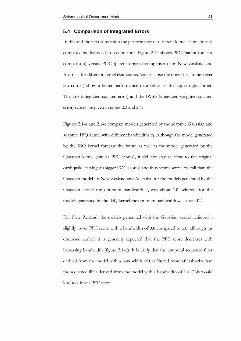
Seismological Occurrence Model 41
5.4 Comparison of Integrated Errors
In this and the next subsection the performance of different kernel estimations is
compared as discussed in section four. Figure 2.14 shows PFC (parent forecast
comparison) versus POC (parent original comparison) for New Zealand and
Australia for different kernel estimations. Values close the origin (i.e. in the lower
left corner) show a better performance than values in the upper right corner.
The ISE (integrated squared error) and the IWSE (integrated weighted squared
error) scores are given in tables 2.3 and 2.4.
Figures 2.14a and 2.14c compare models generated by the adaptive Gaussian and
adaptive IBQ kernel with different bandwidths c1. Although the model generated
by the IBQ kernel forecast the future as well as the model generated by the
Gaussian kernel (similar PFC scores), it did not stay as close to the original
earthquake catalogue (bigger POC scores) and thus scores worse overall than the
Gaussian model. In New Zealand and Australia, for the models generated by the
Gaussian kernel the optimum bandwidth c1 was about 1.0, whereas for the
models generated by the IBQ kernel the optimum bandwidth was about 0.4.
For New Zealand, the models generated with the Gaussian kernel achieved a
slightly lower PFC score with a bandwidth of 0.8 compared to 1.0, although (as
discussed earlier) it is generally expected that the PFC score decreases with
increasing bandwidth (figure 2.14a). It is likely that the temporal sequence filter
derived from the model with a bandwidth of 0.8 filtered more aftershocks than
the sequence filter derived from the model with a bandwidth of 1.0. This would
lead to a lower PFC score.

42 chapter 2
a)
New Zealand
0
1
2
3
52.0 52.5 53.0 53.5 54.0POC (ISE)
PFC
(IW
SE)
GaussianIBQ
b)
New Zealand
1.4
1.6
1.8
2.0
51.5 52.0 52.5 53.0 53.5 54.0POC (ISE)
PFC
(ISE
)
globaladaptive
0.51.0
2.0
0.6
0.8
1.01.2
0.3
0.50.7
0.60.8
1.01.2
c)
Australia
0
10
20
30
40
50
164 166 168 170 172POC (ISE)
PFC
(IW
SE)
Gaussian
IBQ
d)
Australia
0.6
0.8
1.0
1.2
1.4
164 166 168 170 172
POC (ISE)
PFC
(ISE
)
adaptive
global
0.8
1.0
1.2
0.81.0
1.2
0.2
0.40.6
1.0
2.0
0.5
Figure 2.14: Integrated Errors. Parent Forecast Comparison and Parent Original Comparison scores for New Zealand and Australia with sequence filtering. a) and c) compare the models generated by the adaptive Gaussian kernel and adaptive inversbiquadratic kernel. b) and d) compare the models generated by the adaptive Gaussian kernel and global Gaussian kernel. The numbers represent the bandwidths.

Seismological Occurrence Model 43
PFC (IWSE)
PFC (ISE)
POC (ISE)
without sequence filtering
Gaussian 0.8 adaptive 307.39 2.99 Gaussian 1.0 adaptive 243.90 4.78 Gaussian 1.2 adaptive 178.80 6.73
with sequence filtering
Gaussian 0.5 global 1.95 52.03 Gaussian 1.0 global 1.81 52.13 Gaussian 2.0 global 1.55 52.76
Gaussian 0.6 adaptive 2.32 1.66 52.27 Gaussian 0.8 adaptive 1.08 1.61 52.18 Gaussian 1.0 adaptive 1.32 1.51 52.11 Gaussian 1.2 adaptive 1.04 1.53 53.59
IBQ 0.3 adaptive 2.45 52.85 IBQ 0.5 adaptive 1.12 53.32 IBQ 0.7 adaptive 0.69 53.69
Table 2.3: PFC and POC scores for New Zealand.
PFC (IWSE)
PFC (ISE)
POC (ISE)
without sequence filtering
Gaussian 0.8 adaptive 230.62 4.82 Gaussian 1.0 adaptive 188.26 8.47 Gaussian 1.2 adaptive 153.89 20.57
with sequence filtering
Gaussian 0.5 global 1.30 165.43 Gaussian 1.0 global 1.17 167.39 Gaussian 2.0 global 0.80 170.73
Gaussian 0.8 adaptive 4.02 1.03 165.54 Gaussian 0.9 adaptive 3.10 1.06 165.57 Gaussian 1.0 adaptive 2.53 1.12 165.72 Gaussian 1.1 adaptive 2.17 1.18 166.02 Gaussian 1.2 adaptive 1.90 1.25 166.48
IBQ 0.2 adaptive 39.38 166.22 0.86 IBQ 0.3 adaptive 7.29 167.08 0.67 IBQ 0.4 adaptive 2.17 168.08 0.56 IBQ 0.5 adaptive 0.94 169.04 0.51 IBQ 0.6 adaptive 0.49 169.90 0.47
Table 2.4: PFC and POC scores for Australia.

44 chapter 2
Figures 2.14b and 2.14d compare models generated by the adaptive and global
Gaussian kernel with different bandwidths. Whereas the adaptive approach
succeeded in minimizing both PFC and POC, the global approach failed in
doing so. For Australia, the PFC score increased with bandwidth for the
adaptive case, contrary to expectation (figure 2.14d). This is due to the fact that
the ISE is dominated by the properties of the tails of the kernel estimation. The
IWSE for the adaptive case was decreasing with increasing bandwidth as
expected (figure 2.14c).
Without sequence filtering the later seismicity model was not forecast very well
by the earlier seismicity model and the PFC scores were large (see table 2.3 and
table 2.4). On the other hand, the earlier seismicity model stayed close to the
original earthquake catalogue and the POC score was very low. This reflects the
fact that the temporal sequences were not removed from the original earthquake
catalogue. However, they did not occur at the same locations in the later
seismicity model as the large PFC score shows.
5.5 Comparison of Local Squared Errors
Figure 2.15 shows the seismicity representation for Australia modelled with the
adaptive Gaussian kernel and two different bandwidths for different time
intervals. As predicted, for the higher bandwidth there are less individual
seismicity features in both models and the seismicity features of both models
match better compared to the lower bandwidth, i.e. almost every feature in the
earlier model has a corresponding feature in the later model. The difference
between the earlier and later models for the lower bandwidth is reflected in the
number of (mostly green) clusters in the PFC plots. There are less (but bigger)

Seismological Occurrence Model 45
Bandwidth 0.8 Bandwidth 1.2
1978
-199
0
aI) bI)
1991
-199
6
aII) bII)
PFC
aF) bF)
POC
aO) bO) Figure 2.15. Gaussian kernel models. The probability distribution of crustal earthquakes in Australia (above 50 km) generated by adaptive Gaussian kernel estimation from 1978 to 1990 (I) and from 1991 to 1996 (II) above magnitude 4.0 with bandwidths 0.8 (a) and 1.2 (b). The scale gives the probability of one or more earthquakes per year and area unit. (F) local Parent Forecast Comparison squared error scores. (O) local Parent Forecast Comparison squared error scores.

46 chapter 2
clusters for the higher bandwidth (as expected). Also, the biggest differences for
the higher bandwidth are smaller than those for the lower bandwidth, i.e. they
decrease from red to yellow and from yellow to green with increasing
bandwidth. In the POC plot, there are more differences for the higher
bandwidth compared to the lower bandwidth, which can be seen in the greater
amount of green. The corresponding plots for New Zealand showed similar
results.
Figure 2.16 shows the seismicity representation for Australia modelled with the
adaptive IBQ kernel and two different bandwidths for different time intervals.
The differences between the two models with different bandwidths are similar to
the results with the Gaussian kernel. In contrast to the Gaussian kernel, the IBQ
kernel smeared out the seismicity over space more, while maintaining very local
features that are produced by single earthquakes (the POC plots give an
impression of the corresponding original earthquake distributions if only red and
yellow values are considered). Such behaviour is common for kernels with long
tails (Vere-Jones 1992). For the lower bandwidth, many of the local clusters can
be matched to individual earthquakes in figures 2.16 aI) and 2.16 aII). This leads
to a high PFC score since the earlier model fails to forecast the locations of the
earthquakes in the later model. In the POC plots, the regions of low background
rate in the model show significant differences from the original earthquake
catalogue, which can be seen by the high amount of green, especially for the
higher bandwidth. Thus, the activity of low background rates is highly
overestimated by the model generated by the IBQ kernel, which leads to a high
POC score. The corresponding plots for New Zealand showed similar results.

Seismological Occurrence Model 47
Bandwidth 0.2 Bandwidth 0.6
1978
-199
0
aI) bI)
1991
-199
6
aII) bII)
PFC
aF) bF)
POC
aO) bO)
Figure 2.16. Inversbiquadratic kernel models. The probability distribution of crustal earthquakes in Australia (above 50 km) generated by adaptive inversebiquadratic kernel estimation from 1978 to 1990 (I) and from 1991 to 1996 (II) above magnitude 4.0 with bandwidths 0.2 (a) and 0.6 (b). The scale gives the probability of one or more earthquakes per year and area unit. (F) local Parent Forecast Comparison squared error scores. (O) local Parent Original Comparison squared error scores.

48 chapter 2
Cao et al. (1996) stated that the power law kernel (equation 2.5), which is similar
to the IBQ kernel, should be preferred over the Gaussian kernel for seismicity in
California. Their reasoning is based on their choice of bandwidth for the
Gaussian kernel, which produced an over-smoothed model from the earthquake
catalogue. Whereas the power law kernel might produce better results than the
Gaussian kernel for global kernel estimation, global kernel estimation does not
forecast the future seismicity as well as adaptive kernel estimation. Further,
global bandwidths have to be adjusted to different kernel functions, i.e. the same
bandwidth value for different kernels gives, in general, different effective
bandwidths (for further explanation see e.g. Wand and Jones 1995). This has not
been considered by Cao et al. (1996).
Figure 2.17 shows the seismicity representation for New Zealand modelled with
the adaptive and global Gaussian kernels and with and without temporal
filtering. For the global Gaussian kernel, many local features in both models
cannot be matched, whereas for the adaptive Gausian kernel most local features
can be matched for the two time periods, e.g. around latitude –46°, longitude
171° for the global kernel the five clusters in the earlier time period cannot be
matched to the three clusters in the later time period. In the PFC plots,
differences that appear in the global case (e.g. latitude –46°, longitude 171°) do
not appear in the adaptive case. Thus the earlier seismicity representation
modelled by adaptive kernel estimation better forecasts the corresponding later
seismicity representation compared to the representations modelled by the global
kernel estimation. The differences in the POC plot for the global model are very
similar to the differences for the adaptive model.
Without temporal sequence filtering, the intensity of local seismicity features is
often different in the earlier and later models. In the PFC plot, the differences

Seismological Occurrence Model 49
are mostly due to temporal sequences. For the filtered model, the differences are
much lower and the earlier model can better forecast the later model. The
differences in the PFC plot for the filtered representation reflect real fluctuations
in the recorded seismicity (e.g. the region around Arthur’s Pass, latitude -43°,
longitude 172°, had higher seismic activity during the nineties). In the POC plot,
the differences between the unfiltered model representation and the catalogue
are small compared to the filtered representation and the catalogue, consistent
with the non-removal of aftershocks from the original earthquake distribution.
All the models we used in this study are static in time and do not model any
variations of either global or local seismicity changes in time. However, time-
varying models can be tested with the presented methods as well. To test time-
variance, two time periods of possibly different spatial activity have to be
compared, e.g. it is likely that an earthquake occurrence model derived from the
historical earthquake catalogue would be different from an earthquake
occurrence model based on geological fault information (see chapter three and
four).

50 chapter 2
1962-1990 1991-1997
Ada
ptiv
e G
auss
ian
Tem
pora
l Filt
er
aI) aII)
Glo
bal G
auss
ian
Tem
pora
l Filt
er
bI) bII)
Ada
ptiv
e G
auss
ian
No
Filte
r
cI) cII)

Seismological Occurrence Model 51
PFC POC
Ada
ptiv
e G
auss
ian
Tem
pora
l Filt
er
aF) aO)
Glo
bal G
auss
ian
Tem
pora
l Filt
er
bF) bO)
Ada
ptiv
e G
auss
ian
No
Filte
r
cF) cO)
Figure 2.17. Comparison of kernel models. The probability distribution of crustal earthquakes in New Zealand (above 40 km) generated by adaptive Gaussian kernel estimation with temporal sequence filter (a), global Gaussian kernel estimation with temporal sequence filter (b), and adaptive Gaussian kernel estimation without temporal sequence filter (c) from 1962 to 1990 (I) and from 1991 to 1997 (II) above magnitude 4.0. (F) local Parent Forecast Comparison squared error scores. (O) local Parent Original Comparison squared error scores.
52 chapter 2
6 Summary
The comparison of different kernel estimations provided the following results:
• Global kernel estimation performs worse than adaptive kernel
estimation, because it cannot forecast the future seismicity as well as
adaptive kernel estimation, while staying as close to the original
earthquake distribution. Models produced with small global
bandwidths fail to forecast the location of future earthquakes,
especially in regions of low activity, whereas models produced with
high global bandwidths do not stay close to the seismicity
distribution of the original earthquake catalogue. It can be concluded
that global kernel estimation is not useful for the construction of
earthquake occurrence models.
• The Gaussian kernel seems to better forecast the location of future
earthquake activity compared to the IBQ kernel, while staying closer
to the original earthquake distribution. The long tails of the IBQ
kernel dominate the calculation of c2(xi). As a result, local features
which are produced by single earthquakes, and therefore not seen in
other observation intervals, are still inherent in the seismicity
representation even for high bandwidths, whereas the background
seismicity of low activity regions is too high even for low
bandwidths.
• The global bandwidth c1 = 1.0 seems to provide the best results for
the Gaussian kernel. The choice of bandwidth is connected to the
choice of the size of the cells. The optimum value of one for the
adaptive Gaussian kernel reflects the ‘sensible’ binning of the data.

Seismological Occurrence Model 53
The cell sizes for New Zealand and Australia have been chosen in a
way that they are comparable to the sizes of the seismicity features.
• Models with temporal sequences filtered out forecast the locations of
future earthquakes better than unfiltered models. Although the
unfiltered models stay closer to the distribution of the original
earthquake catalogue, temporal sequences should be filtered, because
they lead to an over- or under-estimation of local activity rate. The
closeness of the unfiltered model to the original distribution reflects
the fact that the temporal sequences have not been removed from
the original distribution. After a main shock occurrence model has
been produced, temporal sequences may be incorporated using an
appropriate occurrence model for these sequences (e.g. Omori’s law
for aftershocks).
Using adaptive kernel estimation with temporal sequence filtering on the
historical earthquake catalogue of New Zealand provided the following results
for earthquake occurrence:
• Whereas shallow earthquakes are mostly part of temporal earthquake
sequences (such as main shocks with aftershocks), the subducting
slabs in New Zealand has been nearly free from temporal activity
variations for the last forty years, suggesting that deep earthquakes in
New Zealand do not produce many multiple events, as observed in
the past.
• The probability distribution of main events has been stable in New
Zealand during the last forty years.

54 chapter 2
• No spatial high activity clusters have been observed to decrease to
background activity during the observation time. I infer that there is
a higher risk of the occurrence of medium to large earthquakes
associated with these clusters during the short to medium term (a
few years to decades).
These results will be discussed in further detail when the seismological
occurrence model is compared to the geological occurrence model in chapter
four.

c h a p t e r 3
GEOLOGICAL OCCURRENCE MODEL
Earthquake occurrence models inferred alone from historical earthquake
catalogues can only be expected to be useful for short to medium time intervals
(i.e. not longer than the historical observation time, which is typically about a
hundred years). Since the return times of individual fault ruptures are generally
longer than the time span during which earthquakes have been recorded (even
very active faults have, in general, return times of a few hundred years),
geological information has to be considered when an occurrence model for
longer time periods is developed. Information about regional earthquake
occurrences over the last few thousand years can be obtained from compilations
of mapped, active faults. Such information only includes the largest mapped
surface ruptures.
In fault compilations several measured parameters of individual faults, such as
mapped fault trace and measured single event displacement are recorded (it is
often assumed that faults have a similar displacement for each rupture, e.g.
Schwartz and Coppersmith 1984). To test if the recorded fault parameters (that
are mostly acquired by geological studies) match the observed source parameters
of earthquakes from the last century, the source parameter scaling relationships
of these earthquakes have been revised. The results of this study can be found in
appendix one and are reviewed in section one of this chapter.
The fault compilation used for this study is discussed in section two. In this
section the numerous problems of the parameters of mapped, active faults are

56 chapter 3
reviewed. Further, the source parameter scaling relationships discussed in section
one are used to detect inconsistencies in the recorded parameters of the fault
compilation. It is then explained how these inconsistencies can be corrected.
In section three a ‘dynamic stochastic fault model’ is introduced. This model has
been developed in this study in an attempt to overcome the numerous problems
connected with the geological fault parameters. These problems would bias any
earthquake occurrence model if not taken into account. The results of using this
model for the generation of earthquake occurrence models are discussed in
section four.
Every earthquake occurrence model has to be consistent with the theoretical
plate deformation rates. The moment release rates from the fault simulation have
been converted into slip rates and compared to deformation rates predicted by
plate tectonics in section five.
1 Earthquake Source Parameters
Since faults are the sources of earthquakes, the parameters of the fault
compilation (i.e. fault length, single event displacement, etc.) have to match the
earthquake source parameter relationships (i.e. seismic moment M0, rupture
length L, rupture width W, and displacement d) that have been inferred from
earthquakes from the last century. Since previous authors have come to different
conclusions about how earthquake source parameters scale with each other (e.g.
Scholz 1982, Romanowicz 1992, Wells and Coppersmith 1994), the scaling
relationships have been re-examined in the framework of this project. For that
purpose, the databases of several past studies have been combined and analysed
with appropriate statistics. This new study has been published (Stock and Smith

Geological Occurrence Model 57
2000) and can be found in appendix one. The results that are important for
testing the recorded parameters of the fault compilation are summarized here.
Some additional work on source parameter relationships is presented here as
well.
1.1 Scaling Relationships
Kanamori and Anderson (1975) introduced the concept of self-similarity of
earthquakes based on their observation that the mean aspect ratio L/W and mean
strain drop d/L are constant (i.e. any deviation from the mean is due to scatter)
for all earthquake sizes (see also Abercrombie 1995). Purcaru and Berckhemer
(1982), Scholz (1982), and Scholz et al. (1986) found a breakdown of self-
similarity (the aspect ratio grows with magnitude for large earthquakes) which
can be explained by the finiteness of the width of the seismogenic layer, which
limits rupture width (Pacheco et al. 1992). Whereas Scholz (1982) found that
stress drop stays constant, Romanowicz (1992) inferred from her data set that
rupture width limits displacement and thus stress drop is not constant for large
earthquakes (see also Scholz 1994a, Romanowicz 1994, Scholz 1994b, and Pegler
and Das 1996). The newer study of Wells and Coppersmith (1994), to the
contrary, could not find any breakdown of self-similarity.
After re-examining the data, I found that large dip-slip and strike-slip
earthquakes scale in a different way. Self-similarity breaks down for strike-slip
earthquakes, but not for dip-slip earthquakes. Although this was observed earlier
(e.g. Purcaru and Berckhemer 1982), it had been explained by a wider ranger of
widths for dip-slip earthquakes (Scholz et al. 1986). I could not find any deviation
from a mean constant strain drop for dip-slip earthquakes of all sizes and
regions, and suggest that, for dip-slip earthquakes, the maximum possible

58 chapter 3
rupture width is limiting rupture length and displacement, and hence magnitude.
In contrast, as shown in previous studies (e.g. Purcaru and Berckhemer 1982,
Scholz 1982), the length of strike-slip earthquakes is not limited by width and
thus they can grow long, which leads to increasing aspect ratios.
The resulting scaling relationships between seismic moment and rupture length
are:
log M0 ∼ 3 log L , for dip-slip and small strike-slip and (3.1)
log M0 ∼ 2 log L , for large strike-slip.
Romanowicz’s (1992) findings, that rupture width limits displacement, have been
clearly rejected by my study. Nonetheless, there is the possibility that rupture
area, rather than rupture length alone, limits displacement (e.g. Gross 1996).
Another possibility would be a breakdown of strain drop constancy for very long
faults (e.g. Scholz 1994b). Since the influence of rupture width on displacement
is yet not completely resolved, I assume a constant strain drop for the rest of this
study (following the principle of Ockham’s razor by choosing the simplest
model consistent with the data).
1.2 Frequencies
To be able to estimate earthquake magnitude from a given rupture length, the
mean ratio log (M0 / L3) (for dip-slip and small strike-slip) and log (M0 / L2) (for
large strike-slip) is used. For this purpose, I have studied the frequency
distribution of these ratios (see figure 3.1a). All frequency distributions are
approximately log-normal. The logarithmic mean ratio for dip-slip and small
strike-slip earthquakes is 14.8 ± 0.8, and for large strike-slip earthquakes 16.0 ±

Geological Occurrence Model 59
0.4. For simplicity, I used 15.0 and 16.0 respectively to estimate earthquake
magnitudes from rupture lengths in this study (see equation 3.2).
0.0
0.1
0.2
0.3
0.4
13.8 14.4 15.0 15.6 16.2 16.8log (M0/Ln)
freq
uenc
y
strike-slip smallstrike-slip big
a0.0
0.1
0.2
0.3
0.4
8.E+03 2.E+04 5.E+04 1.E+05L/d
freq
uenc
y
normalreversestrike-slip
b
Figure 3.1: Source Parameter Frequency Distributions. a) Seismic moment [Nm] to rupture length ratio [km] distribution for different faulting mechanisms. n is 3 for dip-slip and small strike-slip earthquakes, and 2 for large strike-slip earthquakes. b) Rupture length [m] to displacement ratio [m] distribution for different faulting mechanisms. The black line is the log-normal distribution N(4.6, 0.2), which is shown for reference. (The green and the red line show normal and reverse earthquakes respectively in both plots.)
Further, I have studied the rupture length to displacement ratio. The frequency
distribution of this ratio is log-normal for all faulting mechanisms (see figure
3.1b). This strengthens the argument that displacement scales with rupture
length. If displacement would scale with rupture width, there would be a tail in
the distribution of the strike-slip earthquakes (similar to the aspect ratio, see
figure A1.6). This tail would indicate a decreasing strain drop with rupture
length. The mean of the logarithmic ratio log(L/d) is 4.6 ± 0.4, which corresponds
to a mean ratio L/d of about 4 x 10⁴.
The scatter of the L/d ratio is rather big (although reasonable for the logarithmic
ratio). It is a mixture of the measurement uncertainty of each rupture length and
displacement and true fluctuations in stress drop (e.g. regional effects, random
behaviour). Under the expectation that the measurements of rupture length and
displacement are more accurate in recent years and the measurement uncertainty
decreases systematically with time, the decrease could be projected into the

60 chapter 3
future. When the predicted measurement uncertainty becomes very small at
some point in the future, the true fluctuation of stress drop could be estimated. I
have studied the logarithmic mean ratio and standard deviation for different time
intervals (see figure 3.2). Whereas the mean ratio stays approximately constant,
the standard deviation is slightly decreasing if very small events are omitted. The
reasoning behind the exclusion of very small events is that the errors in the
measurements of rupture length and displacement are proportionally bigger for
smaller earthquakes. Since the proportion of small earthquakes is increasing in
recent decades the inclusion of these events would lead to a bias in uncertainty.
Since the scatter is very large for all time periods, the true fluctuations of strain
drop could not be estimated, but it is not likely to be above ± 0.25 for the
logarithmic ratio. It could still be below this value if it only reflects the scatter
due to measurement uncertainties.
mean (length / slip)
1.0
1.2
1.4
1.6
1.8
2.0
1800
1900
1930
1940
1950
1960
1970
1980
year
log-
mea
n
a
sigma (length / slip)
0.0
0.2
0.4
0.6
0.8
1.0
1800
1900
1930
1940
1950
1960
1970
1980
year
log-
sigm
a
b
Figure 3.2: Rupture Length to Displacement Ratio in Time. Logarithmic rupture length [m] to displacement [m] mean (a) and standard deviation (b) are plotted for different time intervals. The values indicated by the red squares include all events. For the green dots small earthquakes (L < 10 km, d < 0.1 m) have been excluded.
1.3 Summary
A summary of the source parameter relationships I found in this study follows.
To estimate seismic moment from rupture length I used the following
relationships:

Geological Occurrence Model 61
log M0 [Nm] = 15 + 3 log L [km] , for dip-slip and small strike-slip and
(3.2)
log M0 [Nm] = 16 + 2 log L [km] , for large strike-slip.
The moment magnitude is defined by (Hanks and Kanamori 1979):
(3.3) MW = 2/3 (log M0 – 9.1 ) .
To estimate displacement from rupture length I used the following relationship:
L [m] = 4 x 10⁴ d [m] . (3.4)
The rigidity of the elastic medium μ is defined by (e.g. Aki and
Richards 1980, 53):
(3.5) μ = M0 / L W d ,
From figure A1.6 a mean aspect ratio L/W of about 1.5 can be estimated.
Together with the other scaling relationships this implies a mean rigidity of
μ = 6 x 10¹⁰ Pa. The rigidity of surface faulting is typically given by μ = 3 x 10¹⁰ Pa
(e.g. Bonilla et al. 1984), and rigidity increases with depth. Since the rigidity of
μ = 6 x 10¹⁰ Pa inferred from the estimated source relationships (equations 3.2
and 3.4) is reasonably close to the observed rigidities (considering that a small
change in equations 3.2 or 3.4 would lead to a big change in μ), it can be
concluded that the estimated source relationships fit the ‘true’ source
relationships relatively well (i.e. within 0.3 in log μ). The source relationships of
some studies (e.g. Wells and Coppersmith 1994) cannot be combined in this
way. They rather give mean relationships between pairs of parameters and are
not interested if the estimated source relationships fit together. The advantage of

62 chapter 3
my approach is that regional effects like higher stress drop or lower rigidities can
be incorporated by correcting individual source relationships.
A very recent study of Mai and Berora (2000) revised the scaling relationships of
Wells and Coppersmith (1994) and their source scaling relationships between
magnitude, length, and width agree very well with my results within the error
limits. As in this study, their rupture length to displacement relationship shows a
very high uncertainty, but their findings also reject the scaling relationship found
by Romanowicz (1992).
2 Parameters of Mapped Active Faults
To test the methodologies developed in this chapter a fault database of
reasonable quality is needed. The perfect database would include independently
observed fault parameters (such as mapped fault length and slip rates), a
complete map of active faults that produce earthquakes above a certain
magnitude (for example magnitude seven), and quantitative uncertainties for the
observations. However, such a database does not exist for New Zealand. Given
the complexity of the fault distribution in New Zealand, and the limitation that
only surface ruptures are accessible, it has to be questioned if such a database
can be produced within the near future.
However, to validate any hypothesis about earthquake occurrence, it has to be
falsifiable and tested against a fault database. The recent national fault
compilation of Stirling et al. (1998) has been used for this study (see appendix
two). This fault compilation includes fault parameters for a majority of mapped,
active faults in New Zealand. For each fault a simplified fault trace, magnitude,
and mean return time (recurrence interval) are given. If known, slip rate and

Geological Occurrence Model 63
displacement are also given. The data have been mainly compiled from other
studies. If no observed values for magnitude or return time were known, those
parameters were inferred from other known parameters. For a detailed
description of each fault parameter see Stirling et al. (1998). For a brief discussion
of the fault parameters see appendix two.
It should be noted that the database of Stirling et al. (1998) may have not
recorded all fault traces of large earthquakes and also often inferred magnitude
and return time from single event displacements and fault lengths (see Stirling et
al., 1998, and appendix two). The inference of magnitude and return time does
not introduce any bias, if the regressions used to calculate these values are
correct.
Each fault in this compilation is treated characteristically, i.e. it is expected that
the recorded values of every individual fault are the same for each rupture (see
subsection 2.2). I have removed the subduction interfaces from the compilation,
since the main goal is the comparison of surface braking faults and recorded
crustal earthquake activity. In the compilation, the Taupo Volcanic faulting zone
has been simplified to two faults. This simplification will affect earthquake
occurrences in this zone, and although the two faults are used in this study, the
results should be treated with care (or ignored).
2.1 Fault Parameter Sampling Biases
When measuring fault parameters, there are a lot of difficulties involved that lead
to biases in the recorded fault parameters. The major difficulties and sampling
biases are discussed in the following:

64 chapter 3
• Wells and Coppersmith (1994) observed that for earthquakes in the
last century the surface breaks are systematically smaller than the
subsurface rupture length for all faulting mechanisms. This effect
increases for smaller earthquakes, but is not linear since few small
earthquakes produce surface breaks similar to the subsurface rupture
length. If uncorrected surface lengths were used as an estimate for
true rupture lengths, rupture lengths would be consistently
underestimated.
• Since for smaller earthquakes the surface break decreases, the chance
of not detecting individual faults increases with decreasing surface
length / magnitude (even some earthquakes above magnitude seven
show barely any surface breaks and can be missed; one good
example is the Wairarapa, 1942, earthquake with a surface wave
magnitude of 7.2 and no surface break, Downes et al. 1999).
Additionally, old surface breaks could have vanished over time, for
example by erosion. Although all faults that generate moderate
earthquakes could possibly be detected (e.g. Lettis et al. 1997),
resources for such studies are mostly lacking. Thus, it has to be
determined above which magnitude (fault length) all faults in an area
have been mapped (e.g. Cameron 1997).
• Not all faulting areas are equally mapped, with some areas being well
mapped while others have been scarcely studied. This has an impact
on the completeness of mapped faults. But also fault lengths can be
in error, where some faults have been only mapped within a region

Geological Occurrence Model 65
but not beyond it. There is always the possibility that such faults
continue and are longer than mapped (e.g. Nicol et al. 1996).
• Single event displacements are often measured only on the surface.
The displacement varies along the length of the fault with higher
values to the middle and lower values towards the tips of the fault.
Since the tips are usually buried under the surface, the geologically
measured average displacement tends to be higher than the true
average displacement of the whole fault trace. On the other hand,
the maximum of the displacement lies under the surface, leading to a
geological underestimation of average displacement. These sampling
errors lead to a high uncertainty in the average displacement (Wells
and Coppersmith 1994 studied the relationship between surface
displacement versus subsurface displacement and found that the
uncertainty of average displacement is indeed high). Similar sampling
biases are attached to displacements that are measured in trenches
dug at a fault.
• Another sampling bias occurs when one fault trace that produced
one event in the past has been mapped as two separate faults (i.e. the
middle of the fault has not been mapped). This will firstly have an
effect on the estimated displacement, which will be too high for the
two short faults. Further, the magnitude (inferred from a too short
fault length) will be too low and it will be inferred that there will be
more earthquakes produced in the same area and time interval. The
linkage of two faults that produce separate earthquakes would have
the opposite effect. The possibilities of individual mapped fault

66 chapter 3
segments joining or rupturing separately will be discussed in
subsection 2.2.
• In the fault compilation used in this study earthquake magnitudes are
mostly inferred from fault area (and thus fault lengths) and / or
observed displacements. All sampling biases in the measured fault
parameters will determine the (in)accuracy of the estimated
magnitude. For example, since fault lengths are usually mapped too
short, the estimated magnitude that the faults would produce will be
too low, if inferred from the uncorrected fault length (e.g. Stirling et
al. 2000).
• The distinction of whether a fault is active or inactive is usually made
by reference to a fixed time interval (125,000 years for New Zealand,
Mark Stirling, pers. comm.). As shown in subsection 4.6 the fault
compilation does not include many faults with return times longer
than 20,000. It is possible that many of the faults with return times
longer than 20,000 have been classified as inactive (or are not
mapped at all). For example, the White Creek fault, which has an
estimated return time of 34,000 years), has not been recognised as an
active fault until the Buller, 1929, earthquake, which ruptured this
fault (Berryman 1980). If a lot of faults with long return times have
been classified as inactive the fault compilation is under-sampled.
This effect has the biggest impact in regions where there are
numerous faults and the return times of these faults are long in
general (e.g. North West Nelson). Such a region might have an

Geological Occurrence Model 67
earthquake occurrence rate that lies well above the occurrence rate
estimated from fault activity.
• Earthquake occurrence rates do not follow Poisson statistics, but are
rather clustered in space and time (Kagan and Jackson 1991) and the
variations in the individual return times are high as they are
influenced by fault interactions (e.g. Becker and Schmeling 1998).
This can have implications for the estimated return time for
individual faults. If a fault has been more active than average over
the time in which events have been dated, then the estimated return
time will be too short. Similarly, too long return times will result for
faults that have been less active than average over the time interval in
which events have been dated.
2.2 Characteristic versus Uncharacteristic Behaviour
Schwartz and Coppersmith (1984) found that some faults rupture with similar
earthquake source parameters every time they produce an earthquake, i.e. the
same fault segment ruptures over and over again and produces similar
displacements for each individual rupture. They called such behaviour
‘characteristic’ and proposed that many faults behave in this fashion. Such a
model allows the construction of earthquake occurrence models directly by using
the observed fault parameters without any modification (once sampling biases
are corrected).
More recent studies question the characteristic earthquake model. Newer data
shows that the faults studied by Schwartz and Coppersmith (1984) have variable
rupture patterns and faults behave ‘uncharacteristically’ (e.g. Grant 1996).
Schwartz (1999) has shown that large subduction zones behave

68 chapter 3
‘noncharacteristically’. For the rest of this study, I define the ‘uncharacteristic
model’ to exclude any characteristic fault behaviour. In the uncharacteristic
model, each segment changes its behaviour over time and sometimes joins other
segments to produce bigger earthquakes with higher displacements and longer
return times, rather than consistently producing similar source parameters. The
‘noncharacteristic model’ is defined here to allow a mixture of both characteristic
and the uncharacteristic behaviour. The uncharacteristic and noncharacteristic
models produce a different earthquake occurrence model from the characteristic
model since they allow for a much greater variability of earthquake magnitudes
and return times.
2.3 Faults versus Earthquake Sources
The fault parameters of the fault compilation used in this study have to be
consistent with the earthquake source relationships discussed earlier (equations
3.2 and 3.4). Any deviations will indicate sampling biases in the fault compilation
(or a consistent deviation of earthquakes in New Zealand from the world
average). To develop an earthquake occurrence model based on fault
information, magnitude, return time, and location (i.e. the fault trace) of a fault
have to be known. The magnitude can be directly inferred from rupture length
(equations 3.2 and 3.3). The mean return time T can be inferred from:
(3.6) T = d / σ ,
where σ is the slip rate and the displacement d can be inferred from rupture
length (equation 3.4). If the rupture length could be inferred from the mapped
fault trace (i.e. the mapped length of the fault), the only parameters needed for
the development of an occurrence model would be fault trace and slip rate, since
the other parameters could be calculated with those two parameters. The slip

Geological Occurrence Model 69
rate is a geological constraint that both the characteristic and the uncharacteristic
model have to satisfy. Both models would treat mapped fault traces differently.
The characteristic model would use the fault traces as they were mapped (apart
from length corrections), whereas the uncharacteristic model would allow
different fault traces to join or to break into separate segments.
It has to be noted that, by inferring return times and magnitudes from rupture
lengths, it is assumed that all faults follow the mean behaviour of earthquake
sources. This may not be appropriate for individual faults, since they might
significantly deviate from the ‘normal’ behaviour. However, parameters for
individual faults are mostly very uncertain (any deviation could reflect sampling
biases), so it is not clear how much faults deviate from the mean fault behaviour.
Random deviation from the mean source parameters could be modelled by
including the uncertainties in the source parameter relationships. Since the main
goal here is to establish a mean behaviour of fault rupture, the uncertainties have
not been taken into account. Although regional differences in the source
parameters relationships could not be found (see appendix one), there is still the
possibility that faults in a particular region deviate systematically from the
average behaviour. To take such a deviation into account, it firstly has to be
clarified how big it is. There is not enough data for New Zealand to find a
statistically significant difference from the average source parameter
relationships.
The advantage of this approach is that rather than having three characteristic
parameters (magnitude, return time, and fault trace), only one characteristic
parameter is left (fault trace). It is fairly easy to convert characteristic fault
lengths into uncharacteristic ones, by allowing different fault traces to join and to

70 chapter 3
break into separate segments. This approach has the additional advantage that
only the sampling bias of fault length has to be corrected, which can be done
with the help of the observed displacements. Both rupture length and
displacement have to fit the scaling relationship found earlier (equation 3.4). Any
deviation from this scaling relationship can be used to correct sampling biases of
fault lengths.
Since the displacement is estimated from a corrected fault length it will also be
‘sampling bias free’ (meaning that it will fit the source scaling). Thus, the
sampling biases of return times will only depend on biases in the slip rate and the
omission of faults (due to ‘missed’ fault traces or faults of very long return
times). Magnitudes will be free of sampling biases, because they are inferred
from corrected fault lengths.
To study how well the compilation of New Zealand fault parameters fit the
observed earthquake source relationships, I have inferred displacements from
given mapped fault traces (equation 3.4) in the fault compilation and compared
those values with the measured displacements. Figure 3.3a shows that the
measured displacements are consistently higher than the displacements inferred
from fault traces, independent of faulting mechanism. Further, when estimating
return times from fault traces and slip rates, those estimated return times are
consistently lower than the observed return times (figure 3.3b).

Geological Occurrence Model 71
Single Event Displacements
1.E
-01
1.E
+00
1.E
+01
1.E
+02
1.E-01 1.E+00 1.E+01 1.E+02measured
theo
retic
al
normalreversestrike-slipoblique
a
Return Times
1.E+
011.
E+03
1.E+
05
1.E+01 1.E+03 1.E+05measured
theo
retic
al
normalreversestrike-slipoblique
b
Figure 3.3: New Zealand Fault Parameters versus Source Parameters. a) Theoretical displacements inferred from fault traces compared to measured displacements from the fault compilation (in meters). b) Theoretical return times inferred from fault traces and slip rates (theoretical displacements) compared to measured return times from the fault compilation (in years).
This behaviour can be explained by two factors. Firstly, as noted beforehand, the
mapped fault traces underestimate the true rupture lengths. This leads to
estimated displacements that are too low if the length of the fault traces is not
corrected. Secondly, for some short faults the observed displacement is very high
(e.g. Alfredton, see appendix two). Such faults have probably ruptured in
conjunction with other faults (e.g. the Alfredton fault might be connected to the
Wairarapa fault). If such a segment ruptured alone it would most likely have had
a significantly smaller displacement. Paleoseismologists might not be able to
identify such small events. Thus it might not be clear how often such a fault
joins another fault and how often it ruptures individually. Further, some small
faults might have ruptured with very small displacements which could not be
resolved as individual ruptures, and therefore several events might have
incorrectly been interpreted as one single event. This would lead to measured
displacements that are consistently too big. There is the possibility that strain
drops are consistently too high for New Zealand, which would lead to a similar
result. However, the strain drop would have to be about three times the average

72 chapter 3
strain drop worldwide. There is not enough data for New Zealand to decide if
the strain drop is consistently higher than the world average.
To correct the underestimation of rupture length from mapped fault traces, I
have firstly tried to match separate faults segments that are likely to connect to
adjacent fault segments. Only faults with the same slip-type (or oblique faults)
were allowed to join. Since the main interest in this study is to develop a fault
model that can be used to generate an earthquake occurrence model, and the
particular hazard model that results is only of secondary interest, I did this
analysis judged on the spatial distribution of the faults alone, using common
sense. For the generation of hazard models such an analysis should be
undertaken by an experienced geologist. I was able to connect most of the strike-
slip faults to at least one other close fault. After establishing all possible
connections between strike-slip faults, I found that for most strike-slip faults the
displacement inferred from the new fault traces to be relatively close to the
observed displacement (see figure 3.4). Two faults with not so good fits are the
Ohariu fault and the Pukerua-Shepherds fault. Both faults most likely continue
offshore where they have not been mapped completely. The agreement between
observed displacement versus displacement inferred from fault traces once faults
that possibly produce ruptures together are connected suggests that mostly I
have connected the faults properly. The remaining scatter could be due to
variances in individual strain drop. This result suggests that the rupture lengths
of strike-slip faults do not necessarily need to be corrected for New Zealand. It
is still possible though that some strike-slip faults have been missed or are not
fully mapped. Since the regions that have strike-slip faults have been mapped
fairly well in New Zealand, the lengths of strike-slip faults are not corrected in
this study. It is assumed that if individual faults are allowed to join, the resulting

Geological Occurrence Model 73
earthquakes match the true occurrence rate reasonably well. Since the horizontal
and vertical displacements are not recorded in the fault compilation, oblique
faults have been treated similarly to strike-slip faults, because most of the oblique
faults in the fault compilation have a significant strike-slip component. Oblique
faults follow source parameter relationships that are in between the relationships
of strike-slip and dip-slip faults (see figure A1.4).
0
2
4
6
8
0 2 4 6 8measured
theo
retic
al
Ohariu
Pukerua-Shepherds
Figure 3.4: Theoretical versus Measured Displacements for Strike-Slip Faults. Theoretical displacements inferred from fault traces compared to measured displacements from the fault compilation of strike-slip faults after individual faults have been linked (in meters).
Only a few normal and reverse faults could be connected with other fault
segments. To correct rupture lengths for these faults, the observed lengths (fault
traces) have been compared with the lengths inferred from observed return
times and observed displacement (figure 3.5). With the help of equation A1.3
and A1.4 lines with the slopes 0.78 ± 0.47 for normal and 0.13 ± 0.71 for reverse
faults could be fitted through the data points. For the normal faults a slope of
1/2 has been chosen instead because most data point lie on this slope, which is
within the error limit. The slope for the reverse faults is very steep and probably
caused by the fact that even short faults have very large displacements and thus
there are no data for small displacements. A slope of 1/3 has been chosen
instead, which seems to fit the data reasonably well (considering the quality of

74 chapter 3
the data, see page 74). For both slopes the uncertainty is very high. For these
slopes corresponding intercepts of 0.91± 0.09 for normal and 1.59 ± 0.71 for
reverse faults have been calculated.
Normal Faults
110
100
1000
1 10 100 1000inferred length
mea
sure
d le
ngth
North NIWest NIConnectedEast NI FZ
Edgecumbe
Reverse Faults
110
100
1000
1 10 100 1000inferred length
mea
sure
d le
ngth
South NIHawkes BayNorthwest SICentral + South SIMarlborough
Figure 3.5: Length Correction. Measured length from the fault catalogue compared to length inferred from observed return time and displacement (in km). The dark red line corresponds to the correction relationships (equations 3.7).
The following two linear relationships have been used to correct the fault lengths
of normal and reverse faults:
log Λ = 0.9 + 1/2 log L (normal faults) (3.7)
log Λ = 1.6 + 1/3 log L (reverse faults),
where Λ is the corrected length and L is the measured compilation length. These
relationships are only valid for the correction of geologically measured fault
traces in New Zealand. This result does not contradict the findings of Wells and
Coppersmith (1994) that there are no linear relationships between observed
surface and subsurface rupture lengths. The data from Wells and Coppersmith
(1994) are collected from observed earthquakes and sometimes the surface
rupture length from small earthquakes matches the inferred subsurface length
very well. For the geological data of New Zealand small faults are represented by

Geological Occurrence Model 75
a surface break that is systematically too low. Hence, the difference between this
work and the study of Wells and Coppersmith (1994) is the difference in
accuracy between observed rupture rupture length and mapped fault length.
The need for such a correction is based on the assumption that the surface break
is much smaller for small earthquakes than for larger earthquakes. An alternative
interpretation of the data would be a high strain drop for New Zealand
earthquakes. However, in figure 3.5 for the large earthquakes the observed
surface break is relatively close to the estimated rupture length. It can be
expected that for even larger earthquakes the match of the observed and inferred
rupture length would be very close.
For the normal faults, apart from the five faults from the East North Island
Fault Zone and the Edgecumbe, 1987, earthquake, all faults follow the linear
relationship very well (figure 3.5). The five faults from the east North Island fault
zone probably continue offshore and thus are longer than mapped. The
Edgecumbe fault trace has been revised in a newer fault compilation and is
mapped as longer now. It has to be noted that Edgecumbe is the only ‘modern’
measurement. However, this shouldn’t be overemphasised given the scatter of
modern observations (see figure A1.2). Additionally, the purpose of the
correction is to match measured displacement and length of paleoseismic events.
Since Edgecumbe isn’t a paleoseismic event, it shouldn’t be included anyway.
The scatter is much bigger for the reverse faults and a linear trend is not as
obvious as for the normal faults. The four shortest faults deviate the most. The
Inangahua, 1968, earthquake has an observed average displacement of 40 cm.
Since the earthquake had a surface wave magnitude of about 7.4 (Anderson et al.
1994) this displacement seems to be underestimated. The fault was probably

76 chapter 3
much longer and had a much higher subsurface displacement. For the Lyell fault,
Blue Mountain fault, and Spy Law fault the fault trace has been used to calculate
the return time in the fault compilation. Since the fault trace is likely to be too
short, the return times are probably too short as well. Thus, the inferred fault
lengths should be longer. When these four faults are taken out of the analysis the
scatter is still large, but the general trend is that reverse faults are mapped much
too short. For example, a rupture length of about 100 km has an average surface
break of only 20 km (see figure 3.5). Thus, the chance of ‘missing’ reverse faults
is very high, even for faults that produce big earthquakes.
Since the surface break of reverse earthquakes is so small compared to the
subsurface rupture length it is possible that the measured displacement along the
surface break is much bigger than the average displacement. This would mean
that the lengths of reverse faults are overcorrected by my correction (equation
3.7). With the help of theoretical rupture models it could be possible to estimate
a relationship between measured surface displacement and average subsurface
displacement. This has not been done in this study since there seem to be further
problems with this type of correction (see discussion in subsection 4.4).
The length corrections discussed above should only be used for New Zealand
faults. In other regions of the world surface fault traces may be preserved better
over time or they might have been mapped more extensively. It will probably be
necessary to revise these relationships for an updated fault compilation for New
Zealand. The length corrections may be related to sampling (e.g. area coverage,
regional accessibility) rather than physical relationships (e.g. rate of erosion,
stress drop).

Geological Occurrence Model 77
In the fault compilation only magnitudes and return times are given for every
individual fault. Since the return time changes when two different faults are
combined to produce a larger event together, the slip rate is needed to estimate a
corrected return time. The missing slip rates have been estimated from observed
displacements or displacements inferred from rupture lengths and observed
return times (equation 3.6, the new slip rates are shown in appendix two). This
procedure is not as accurate as having an observed slip rate, since it has to be
decided if the fault ruptures together with other faults to produce the observed
return time.
3 Dynamic Stochastic Fault Model
One of the problems when developing areal earthquake occurrence models
based on fault information is that earthquakes are represented by the projected
faults onto the surface hence they are represented as line sources. Historical
earthquake catalogues typically only record the hypocentres (point sources), and
the projected epicentres are used for the development of occurrence models. To
compare earthquake occurrence models based on fault information with
occurrence models based on historical earthquake catalogues either the faults
have to be converted to epicentres or the recorded epicentres have to be
converted to faults. Similarly, for a three-dimensional study the fault planes have
to be converted to hypocentres, or vice versa. For this study, I chose to convert
fault lines to epicentres by simulating hypocentres occurring on the mapped,
active faults over a fixed time interval (10,000 years).
It is general practice that the observed fault parameters are taken as the typical
behaviour of a fault and left unchanged for every single rupture of the faults
over the simulation period. Such a model can be called ‘static’ in time and

78 chapter 3
assumes that all faults behave characteristically. I use a ‘dynamical’ model where
individual faults are allowed to produce ruptures together with other faults or
where only part of a fault is allowed to rupture alone. This model is imposing
noncharacteristic fault behaviour. Whether the dynamic fault model will produce
characteristic or uncharacteristic fault ruptures depends on the properties of the
considered faults and the imposed rules that allow or prohibit the linkage of
faults.
3.1 Fault Linkage Based on Angle
To decide whether fault segments that are mapped as one fault in the fault
compilation produce single or compound ruptures, the angle (orientation
between both segments) and the gap (distance between segment tips) between
pairs of segments is considered. There are several simulation studies that
estimate the slip distribution for different angles between two fault segments that
rupture together (e.g. Kase and Kuge 1998, Maerten et al. 1999). But there
appears to have been no work investigating the probability for two segments
rupturing together for a given angle between them. The lack of such studies can
be explained by the complexity of fault tip zones. Fault tip zones include
complications such as diffuse breakdown zones (multiple strands), significant
fault bends (‘dog tails’ and ‘rainbows’), and stepovers (e.g. King 1986, Ward
1997b). Since there is no information about the details of the fault tips in the
fault compilation, any complications have to be ignored. For this study, the
orientation between two faults is assumed to be between 0° and 90° degrees.
This choice imposes an equal chance of two faults joining whether the second
fault continues to the ‘left’ or ‘right’ of the first fault with the same angle, i.e. the
angle between two faults is treated symmetrically. This is not correct, because the
dip direction and the vertical gap (stepover gap) relative to strike direction

Geological Occurrence Model 79
between two segments would probably have an effect on the likelihood of
linkage. Unfortunately, the influence of these asymmetries on the probability of
fault linkage is not known.
To calculate the probability of two segments rupturing together depending on
the angle between them, I use a one-sided standard normal distribution. Firstly, I
draw a random number from a set of numbers between zero and infinity that are
standard normally distributed. I multiply this number with a ‘parameter angle’
(e.g. 90°) and the product gives the ‘cut-off angle’. If the angle between the two
segments is less than or equal to the cut-off angle, the segments produce a linked
rupture. The chance that two segments will produce a linked rupture when the
angle between them is equal to the parameter angle (e.g. 90°) will be 68%. (By
multiplying the drawn random number with the parameter angle I change the
standard normal distribution to a normal distribution with sigma being the
parameter angle). The probability of two segments producing a rupture together
increases with the choice of a bigger parameter angle. In this study, I compared
three different values of parameter angles: 22.5°, 45°, and 90°.
3.2 Fault Linkage Based on Distance
The maximum distance which allows two segments to produce joint ruptures
has been well studied and is typically about 5 to 10 km (Harris et al. 1991, Harris
and Day 1999, Magistrale and Day 1999) or 10% of the total length (An 1997).
The probability of two faults rupturing together for a given distance between
them has, to my knowledge, not been studied. Most likely, this probability
depends not only on the distance (and angle) alone but also on other properties
such as rigidity of the rock, amount of micro-cracks, etc. Since such properties
are not known for faults in the fault compilation, the probability of two

80 chapter 3
segments producing joint ruptures has been calculated using a one-sided
standard normal distribution. The calculation of the probability is equivalent to
the calculation of the probability for a given angle. A drawn random number is
multiplied with a ‘parameter distance’ (e.g. 10% of the total rupture length) to
produce a ‘cut-off distance’. The distance between the two segments has to be
less than or equal to the cut-off distance or a ‘maximum distance’ (e.g. 20 km). A
maximum distance has to be imposed to rule out the possibility that faults that
are far apart could join (as they still would have a very small probability of
joining). Parameter distances of 10% and 20% of total rupture length and
maximum distances of 20 km and 40 km respectively have been used in this
study. Those values may seem a little bit too generous (two faults with a gap of
10% of the total length in-between have a chance of 68% to produce a linked
rupture although this gap length corresponds to the maximum gap length
reported in the literature), but this choice should allow for the fact that the fault
tips might be buried or that a subsurface connection exist between the two
faults.
It should be noted at this point that the choice of parameter angles and distances
may seem a bit generous. However, as discussed in section 4.1, the choice of the
parameters had virtually no effect on the occurrence of earthquakes above
magnitude seven.
3.3 Limits on Fault Linkage
To decide if two segments join, other criteria have been taken into consideration.
Firstly, the fault produced by two segments has to continue into the same
direction. Further, only faults of same slip types are allowed to join. Dip-slip
faults are allowed to link with dip-slip faults that have a strike-slip component

Geological Occurrence Model 81
(e.g. normal faults are allowed to join normal-oblique faults) and strike-slip faults
are allowed to link with strike-slip faults that have a dip-slip component.
Faults with a logarithmic difference of 0.5 (base 10) in slip rate are allowed to
join without any modifications (a logarithmic difference of 0.44 has been
calculated as the scatter in the recorded slip rates in the fault compilation). Faults
where the difference is bigger are allowed to join on a probabilistic basis, with
the chance of linkage being one over the logarithmic difference. This
compensates for the case where the slip rates of two linking faults are very
different. If this would not be done one fault would produce too many
earthquakes while the other one would produce too few earthquakes.
The limit of rupture length by maximum possible rupture width for dip-slip
earthquakes has been considered (see appendix one). Normal faults are
forbidden to have a rupture length over 70 km (which corresponds to a
seismogenic width of 20 km and a dip-angle of about 25°; most normal faults
have a dip-angle of about 50° and few normal faults have dip-angles of less than
20°, Jackson and White 1989). 70 km is the maximum recorded fault length for
normal faults in the fault compilation (see figure 3.5). The maximum rupture
length for reverse faults has been limited to 180 km (which corresponds to a
seismogenic width of 20 km and a dip-angle of about 10°). Reverse faults
generally have lower dip-angles than normal faults and thus bigger rupture
widths (the global distribution of dip-angles of reverse earthquakes is bimodal
with maxima at about 30° and 50°, Sibson and Xie 1998). The northernmost
reverse fault in Hawkes Bay has a corrected rupture width of over 200km and
would produce earthquakes bigger than magnitude 8.5. Since this fault lies
offshore, it is plausible that it has been mapped in a very simplified way. I

82 chapter 3
divided this fault into two equal sized segments, to avoid the generation of
overly large earthquakes from this fault. The limitation of length due to rupture
width does not affect the connection of dip-slip faults very much, because for
most dip-slip earthquakes that are mapped the strike directions are parallel, i.e.
most dip-slip faults lie next to each other perpendicular to the strike direction
rather then in strike direction. The only faults that are forbidden to join by the
imposed length limit are the two simplified faults from the Taupo faulting zone
and the offshore faults in Hawkes Bay. If a more detailed fault compilation were
used, the imposed maximum lengths for dip-slip faults might have to be
changed. It would be of advantage to use the dip-angle of the faults (which are
not known very well) and the local seismogenic thickness to estimate maximum
rupture length.
3.4 Simulation of Fault Activity
The simulation of a cumulated rupture distribution over 10,000 years is done by
a computer program. For the simulation, a spatial distribution of faults is
calculated for each year, i.e. the program decides which fault segments rupture
together and which rupture alone for the particular year. To construct the annual
distribution of fault ruptures, the program starts with the individual fault traces
of the fault compilation. Since the fault traces in the compilation are simplified
and individual segments have been joined, the program checks if the fault trace
should be split into several segments depending on the angle between the
segments of the fault. As explained above, the program draws a random number
from a normal distribution and splits two segments if the angle between them is
bigger than the cut-off angle. Once this has been done for all faults, the distance
between all individual faults is checked. The decision, whether two segments
join, includes several steps. Firstly, the total length of both segments is calculated

Geological Occurrence Model 83
and a probability of both segments joining is calculated, as described above. If
the segments would join, the two angles between each segment and the
intermediate segment that would combine the original segments are calculated
and tested to see if both segments join the intermediate segment. Segments that
have been separated in the first angle test cannot re-join.
Once an annual rupture distribution has been established, the parameters for
each fault are calculated. The slip rates of the joining segments are taken as the
mean, and displacements, magnitudes, and return times are inferred from fault
lengths (see earlier discussion). To separate small and large strike-slip faults
(which has to be done to calculate an appropriate magnitude using equation 3.2),
a fault length of 30 km has been used. The return time is then used to calculate
the probability that the fault will rupture in this particular year. This probability
corresponds to (approximate) Poisson behaviour over time. Faults rupture in
clusters in time and space (Kagan and Jackson 1991), and thus the faults do not
behave as Poisson. Since I am only interested in the mean behaviour of the faults
over a long time (10,000 years), and not in fluctuations with time, Poisson
behaviour can be safely assumed as an average behaviour.
If a fault ruptures, the event is equally distributed over the whole fault so that the
integrated activity over the length of the fault equals one event. This enables the
direct comparison of this model and the earthquake occurrence model based on
the historical earthquake catalogue. Since all faults have different lengths and are
mostly mapped too short, the results can look intriguing. Long faults appear to
have a relatively lower activity over space than short faults. This is correct when
it is assumed that earthquakes are generated by point sources. However, it
appears as though long faults are less active than short faults which is not

84 chapter 3
correct. Further, due to the underestimation of rupture length, the activity of
individual faults should have been distributed over a greater length. Since it is
not known where the fault continues or where the unmapped parts are
(otherwise they would be mapped!), the seismicity has been accumulated on the
mapped part.
4 Results
For different simulations using different sets of simulation parameters,
magnitude frequency distributions have been plotted. Those magnitude
frequency distributions have been compared to the magnitude frequency
distributions of the historical earthquake catalogue. To study the local
earthquake occurrence distribution of different fault simulations, plots of the
simulated fault distribution in New Zealand have been produced. Finally, the
return time frequencies resulting from the simulations have been plotted.
4.1 Magnitude Frequency Distributions
Figure 3.6 shows the magnitude frequency distributions for several simulations
with different simulation parameters (figure 3.6a) and the same simulation
parameter (figure 3.6b). The magnitude frequency distribution of the simulated
fault ruptures behaves approximately as predicted by the Gutenberg-Richter law.
Angle parameters that are more likely to inhibit fault linkage produce more small
earthquakes below magnitude seven than simulation parameters that encourage
fault linkage. However, above magnitude seven the angle parameters seem to
have little influence on the magnitude frequencies, and thus fault linkage. The
two different gap parameters produce very similar results for all magnitudes.
Figure 3.6b shows that the scatter of different simulations with the same
simulation parameters is relatively small. Since the choice of simulation

Geological Occurrence Model 85
parameters does not influence the results of earthquake occurrence above
magnitude seven, the choice of simulation parameters seems to be of little
importance for the construction of an earthquake occurrence model above
magnitude seven based on mapped active faults.
1.E-04
1.E-03
1.E-02
1.E-01
1.E+00
4 5 6 7 8 9magnitude
freq
uenc
y22.5° / 0.145° / 0.190° / 0.145° / 0.2characteristic
a
1.E-04
1.E-03
1.E-02
1.E-01
1.E+00
4 5 6 7 8 9magnitude
freq
uenc
y
b
Figure 3.6: Magnitude Frequencies for Different Fault Rupture Simulations. a) magnitude frequencies for different simulation parameters. Parameter angles of 22.5°, 45°, and 90° and parameter gaps of 10% and 20 km (0.1), and 20% and 40 km (0.2) have been studied. For comparison, the characteristic model is shown. The grey line shows a b-value of one. b) magnitude frequencies for a parameter angle of 45° and a fixed gap of 10% and 20 km for three simulations. The frequencies are given in events per year and are not cumulative.
For comparison, the magnitude frequency of the fault compilation if all faults are
treated characteristically (and are not corrected for length) is shown. It can be
seen that the characteristic model produces significantly fewer earthquakes than

86 chapter 3
the dynamic model. The overall higher activity of the dynamic model can be
explained by the length correction. Since many faults have been corrected to be
longer, they produce either bigger earthquakes, or more small earthquakes if fault
segments rupture independently. The higher activity for large earthquakes could
additionally be explained by the allowance that single faults join and produce
bigger earthquakes. It has to be emphasised though, that the total higher activity
can only be explained by the correction of sampling biases. It is not caused by
the dynamic model alone.
Another important result is the observed maximum magnitude of the simulated
fault ruptures. Over a time period of 10,000 years the dynamic model produces a
maximum magnitude of 8.4, compared to 8.1 in the characteristic model. In
total, the occurrence of magnitude eight and above earthquakes lies well above
the occurrence of magnitude eight earthquakes in the characteristic model.
Earthquakes of that size might be rare but are possible, if one considers a crustal
thickness of 30 km (for example for offshore reverse faults in Hawke’s Bay) and
a possible dip angle of 15°, which would result in a magnitude 8.4 earthquake.
Earthquakes with even lower dip-angles are observed in the Himalayas (Sibson
and Xie 1998).
4.2 Deficiency of Large Strike-Slip Earthquakes
There seems to be a deficiency of strike-slip earthquakes between magnitude
seven and a half and magnitude eight. Between magnitude six and a half and
magnitude seven and a half the number of earthquakes seems to be too high
(considering that some faults with magnitudes above seven have not been
mapped). The gap between magnitude seven and a half and magnitude eight
could possibly be filled in with earthquakes from regions where the fault model
Geological Occurrence Model 87
does not show enough activity to match the activity inferred from the historical
earthquakes (e.g. west Nelson as discussed in chapter four).
This mismatch could be caused by faults that have not been mapped or faults
that have long return times and have been erroneously classified as inactive.
Most likely, smaller faults would (at least) have been overlooked (and not
included in the fault compilation) in the same proportion predicted by the
Gutenberg-Richter distribution as large faults. Additionally, as small faults
produce a smaller surface rupture than large faults, it is even more likely that they
have been overlooked. Thus, the addition of earthquakes between magnitude
seven and a half and eight to the magnitude frequencies would require the
addition of earthquakes below magnitude seven an a half in the same proportion
and raise the already high occurrence rate of earthquakes between magnitude six
and a half and magnitude seven and a half.
It is more likely that some of the earthquakes between magnitude six and a half
and magnitude seven and a half should be bigger, to fill in the gap between
magnitude seven and a half and magnitude eight. This can be achieved if some
faults in the dominant strike-slip regions (i.e. east North Island and
Marlborough) have not been included in the fault compilation. Those faults
would add to the probability of fault segments linking (as that would produce
more possibilities for faults to connect with each other) and the number of
single segment ruptures would decrease in favour of linked ruptures. For
example, a previously unmapped fault could act as a bridge between two mapped
faults that would individually produce magnitude six and a half earthquakes, and
produce a compound fault rupture of magnitude seven and a half (see figure
A1.4).

88 chapter 3
The increase in the probability of segment linkage does not necessarily require
the addition of previously unmapped faults with short return times, but could
also be explained by the inclusion of faults with long return times, that have been
previously classified as inactive. If enough of such faults were added, more large
earthquakes, at the cost of medium-sized earthquakes, will occur. This is an
important result and it will be studied further in the rest of this chapter and the
next chapter.
4.3 Magnitude Frequencies of Historical Earthquakes
Figure 3.7 shows the magnitude frequencies (non-cumulative) for different time
periods of the historical earthquake catalogue compared to the magnitude
frequencies of the dynamic fault model. The same time intervals as in chapter
two section one have been used for the historical earthquakes (see table 2.1). For
the earthquakes before 1942 magnitude frequency plots have been constructed
for individual years equivalent to the methodology in chapter two, section one. A
cut-off magnitude of 7.0 has been found from 1870 onwards. This time
corresponds to the start of organised earthquake reporting in New Zealand. For
the historical earthquake catalogue all magnitude frequencies have a b-value of
about one. The activity level of all time intervals varies, with the nineties being
very active and the earlier decades being less active. The activity of the simulated
faults seems to approximately fit the magnitude frequency distributions of the
historical earthquakes.

Geological Occurrence Model 89
1.E-04
1.E-03
1.E-02
1.E-01
1.E+00
1.E+01
1.E+02
1.E+03
2 3 4 5 6 7 8 9magnitude
freq
uenc
y
1991 - 19951987 - 19901962 - 19861943 - 19611870 - 1942faults
Figure 3.7: Magnitude Frequencies for Different Time Intervals. The magnitude frequencies of different time intervals of the historical earthquake catalogue compared to the magnitude frequency of simulated faults. The simulation parameters are 45° for the angle and 10% and 20 km for the gap. The grey line shows a b-value of one. The frequencies are given in events per year.
The historical earthquake catalogue contains aftershocks and earthquakes related
to the shallow part of the Hikurangi subducted plate below the eastern North
Island. The aftershocks have not been filtered in this analysis, because there is
the possibility that large aftershocks have been recorded in the fault compilation
(as fault offsets), leading to shorter return times for faults on which aftershocks
have been identified as fault breaks. Further, the earthquakes below the eastern
North Island have not been filtered either, because it is possible that they
produce surface ruptures (i.e. the rupture might start at the base and progress
upwards to the surface, e.g. Cole and Lewis 1981), and thus fault breaks would
have been recorded in the fault compilation.

90 chapter 3
1.E-04
1.E-03
1.E-02
1.E-01
1.E+00
1.E+01
1.E+02
1.E+03
3 4 5 6 7 8 9magnitude
freq
uenc
y
earthquakes
faults
strike-slip
characteristic
a
1.E-03
1.E-02
1.E-01
1.E+00
1.E+01
1.E+02
1.E+03
1.E+04
3 4 5 6 7 8 9magnitude
cum
ulat
ive
freq
uenc
y
earthquakes
faults
strike-slip
characteristic
b
Figure 3.8: Magnitude Frequencies. The magnitude frequencies (a) and cumulative magnitude frequencies (b) of the historical earthquake catalogue compared to the simulated faults and characteristic faults. The grey lines show a b-value of one. Strike-slip frequencies include oblique slip events as well. The frequencies are given in events per year.
In figure 3.8 the magnitude frequency distributions of the historical earthquake
catalogue have been joined together. The earthquakes for all years above the
completeness magnitude have been added for that purpose (see table 2.1). The
steps in the magnitude frequency indicate different activity levels for the
different time periods (the b-value is still one as observed in figure 3.7!). The
earthquake activity has increased over the decades since the forties and is highest
in the nineties. The activity in and before the forties was high as well. It has to be
noted that the activity of the historical earthquake catalogue above magnitude

Geological Occurrence Model 91
seven might be slightly underestimated. Firstly, the local magnitude might be
slightly underestimated for large earthquakes (see chapter two, subsection 1.4).
Further, the only historically observed earthquake above magnitude eight
(Wairarapa, 1855) has not been included, as only earthquakes after 1870 have
been included.
The magnitude frequencies from the dynamic model drop below the activity of
the historical earthquake catalogue between magnitude seven and a half and
magnitude eight and rise to the activity level of the historical earthquake
catalogue between magnitude six and a half and magnitude seven. This
behaviour can be explained by missing strike-slip faults (or fault segments) as
discussed in subsection 4.2. The magnitude frequencies of the simulated strike-
slip fault ruptures show that the high activity level between magnitude six and a
half and seven is indeed produced by the strike-slip faults. At about magnitude
seven, the magnitude frequencies of the simulated strike-slip faults drop rapidly
below the magnitude frequencies of the historical earthquake catalogue with a b-
value higher than one. At magnitude eight the activity of the strike-slip faults is
producing relatively more earthquakes than between magnitudes seven and eight,
not following the trend of a b-value greater than one.
As the historical earthquake catalogue clearly follows a b-value of one in the
magnitude range where the strike-slip earthquakes have a b-value of above one,
it is likely that the high b-value is an artefact. If some faults that generated
earthquakes between magnitude six and a half and seven in the simulation would
rather produce earthquakes above magnitude seven and a half, the b-value could
decrease to one, matching the b-value of the historical earthquake catalogue. It is
even possible that some of those faults would sometimes connect in a way that

92 chapter 3
they produce earthquakes of magnitudes above eight. This would mean that the
earthquakes simulated by fault ruptures are not complete above magnitude eight.
Although the strike-slip faults that typically produce earthquakes above
magnitude eight might be mapped completely, the incompleteness of faults that
typically produce earthquakes below magnitude eight (but sometimes are still
able to produce bigger earthquakes) could still cause incompleteness of simulated
strike-slip earthquakes above magnitude eight. The magnitude frequencies of the
simulated strike-slip fault ruptures support the result that there are strike-slip
faults missing in the fault compilation (section 4.2).
The magnitude frequencies generated by the characteristic fault model do not
match the magnitude frequencies of the historical earthquakes as it clearly
generates too few earthquakes for all magnitudes. The magnitude frequencies
from the characteristic model are very similar to the simulated magnitude
frequencies from the strike-slip fault ruptures. This means that the characteristic
earthquake model does not seem to be able to generate enough reverse
earthquakes above magnitude seven and a half (i.e. the number of ruptures on
mapped reverse faults does not match the historically observed activity of
reverse earthquakes). The lack of large reverse earthquakes in the characteristic
model will be studied further in the rest of this thesis.
The characteristic model seems to predict too few earthquakes above magnitude
seven and a half. Although the characteristic model produces too few
earthquakes between magnitudes seven and seven and a half it is possible that it
produces too many strike-slip earthquakes if one adds dip-slip earthquakes at
those magnitudes (as the characteristic model seems to not produce enough dip-
slip earthquakes). This is a similar behaviour to the dynamic model which

Geological Occurrence Model 93
predicts too many strike-slip earthquakes between magnitudes six and a half and
seven (compared to the historical earthquakes which include dip-slip
earthquakes) and too few earthquakes above magnitude seven and a half. This
suggests that the problem of missing strike-slip faults exists also in the
characteristic model.
An explanation for the cluster of too many strike-slip earthquakes being about
half a magnitude lower in the dynamic model than in the characteristic model is
the allowance in the dynamic model that strike-slip fault segments can rupture
independently. This would lead to systematically lower magnitudes, if there are
not enough possibilities for strike-slip faults to link and produce bigger
magnitudes. Another reason for this difference is the different calculation of the
magnitude for strike-slip faults. In the fault compilation the source scaling
relationships of Wells and Coppersmith (1994) has been often used to calculate
the characteristic magnitude. The source scaling relationships found in this study
imply a lower magnitude for long strike-slip faults (see subsection 3.1). Thus, the
magnitudes of long strike-slip faults are systematically too high in the
characteristic model (for example, the rupture length of an earthquake of
magnitude 7.5 after my source model would correspond to a magnitude of 7.6 in
the Wells and Coppersmith (1994) model).
4.4 Too many Large Dip-Slip Earthquakes
The activity of the dynamic fault model over magnitude eight is higher than the
activity of the historical earthquake catalogue (when extrapolated, figure 3.8). As
the activity based on simulated strike-slip fault ruptures is much lower than the
total simulated activity above magnitude eight and since the normal faults are not
long enough to produce earthquakes above magnitude eight, the high activity

94 chapter 3
above magnitude eight is mainly generated by simulated reverse fault ruptures.
The high activity level could possibly be explained by an over-correction of
length for reverse faults, as discussed in subsection 2.3.
In chapter four it is suggested that dip-slip faults behave uncharacteristically
rather than characteristically. Since the length correction will produce very long
and straight reverse faults, the corrected faults will always produce characteristic
ruptures in the simulation, i.e. the reverse faults will produce ruptures with a
maximum magnitude (and displacement) every time they rupture. They should
be allowed to produce smaller earthquakes as well as large ruptures, which would
decrease the return times (and number) of above magnitude eight earthquakes
and add earthquakes below magnitude eight to the magnitude frequencies. This
behaviour of wrongly corrected reverse faults will be studied further in the rest
of the thesis.
It can be concluded that the methodology introduced in this study generated too
many reverse earthquakes above magnitude eight and too few reverse
earthquakes below magnitude eight. There might be a similar effect for normal
faults, but it will not be as pronounced as the length correction for normal faults
is not as big as for reverse faults and normal faults are not very long (i.e. not
longer than 70 km, see figure 3.5, which corresponds to a magnitude of about
7.0, see figure A1.2).
4.5 Spatial Representation of Fault Ruptures
Figure 3.9 shows the simulated fault activity for two different simulation
parameters, for simulated ruptures over magnitude seven and a half. Both plots
look very similar supporting the previous result that the simulation parameters
do not have a big effect on simulated earthquake occurrence above magnitude

Geological Occurrence Model 95
seven (compare to figure 3.6a). The only difference between both plots can be
seen in the northeast of the North Island (onshore). There is less activity in this
region when the chosen simulation parameters favour single fault segments to
rupture individually (i.e. small parameter angle). Such parameters lead to fewer
big and more small earthquakes, and therefore no earthquakes above magnitude
seven and a half are observed in this region in figure 3.9a.
When comparing figures 3.9a and 3.9b one has to be aware that the dynamic
fault model is a stochastic model and thus subject to random scatter. A good
example is the different activity of the Alpine Fault in figures 3.9a and 3.9b.
Since the Alpine Fault is very straight, the angle parameter has only a small
influence on the rupture distribution of this fault. Therefore, the difference in
activity of the Alpine Fault in both figures is due to random scatter. It is for
example possible that in figure 3.9a the Alpine Fault has ruptured more often in
individual segments. This would decrease the return time of individual ruptures
and would increase the occurrence rate of ruptures on the fault. In contrast, in
figure 3.9b the Alpine Fault produced less but bigger earthquakes over the same
simulation period. All spatial representations of simulated fault ruptures
presented in this study are subject to random fluctuations.

96 chapter 3
a)
b)
Figure 3.9: Simulated Fault Activity for Different Parameters. a) fault activity above magnitude 7.5 with simulation parameters 22.5° for the angle and 10% and 20 km for the gap. b) fault activity above magnitude 7.5 with simulation parameters 90° for the angle and 10% and 20 km for the gap. The colour scale is in events per year.
Figure 3.10 shows the regional simulated fault activity for different magnitude
ranges. As predicted in subsection 4.2, the relative activity in the eastern North
Island (onshore) is decreasing with increasing magnitude. Over a simulation
period of 10,000 years no earthquakes above magnitude eight have been
produced in this region. The decrease in the relative frequency of large
earthquakes in that region could possibly be explained with the back-arc opening

Geological Occurrence Model 97
of the Taupo Volcanic Zone (e.g. Smith et al. 1989). The strike-slip faults change
their direction away from the strike of the plate boundary (e.g. Beanland and
Haines 1998). The change in direction would increase the angles between single
fault segments and lead to a lower number of segment linkages, which would
decrease the number of large earthquakes. Additionally, since the faults are not
orientated parallel to the strike of the plate boundary anymore, any ruptures on
those faults would be less effective in decreasing the accumulated strain caused
by the relative movement of the Australian and Pacific plate. This strain would
rather have to be released by oblique faults to the east.
The activity of the dip-slip faults (e.g. Hawke’s Bay, Otago) above magnitude
eight (figure 3.10b) seems to be too high, as observed beforehand (compare to
figure 3.8 and subsection 4.4). A likely simplification of the reverse faults in
Hawke’s Bay (they have been mapped very straight) and the correction of
rupture length, which produces very long and straight reverse faults (see
discussion in subsection 4.4), are responsible for this high activity. It is much
more likely that a significant number of these earthquakes should have had a
lower magnitude. The activity of the Taupo Fault Zone seems to be too high as
well (figure 3.10a) which can be explained by the simplification of the whole
Fault Zone to two faults in the fault compilation.

98 chapter 3
a)
b)
Figure 3.10: Simulated Fault Activity for Different Magnitude Ranges. a) fault activity above magnitude 7.0 with simulation parameters 45° for the angle and 10% and 20 km for the gap. b) fault activity above magnitude 8.0 with simulation parameters 45° for the angle and 10% and 20 km for the gap. The colour scale is in events per year.

Geological Occurrence Model 99
a)
b)
Figure 3.11: Fault Activity for Strike-slip Faults and Characteristic Faults. a) fault activity for strike-slip and oblique faults above magnitude 7.5 with simulation parameters 45° for the angle and 10% and 20 km for the gap. b) fault activity above magnitude 7.5 based on characteristic earthquakes. The colour scale is in events per year.
Figure 3.11a shows the simulated fault activity for strike-slip and oblique faults.
The activity of the simulated strike-slip fault ruptures seems to be fairly
homogeneous in the South Island. It decreases progressively to the north. As the
magnitude frequencies above magnitude seven and a half are too low for strike-
slip fault ruptures (figure 3.8) this is probably the region where more fault

100 chapter 3
segments should produce compound ruptures (see subsection 4.2). It is possible
that the increasing complexity due to the change in direction of the strike-slip
faults on the North Island not only lowers the occurrence of large earthquakes,
but increases the chance of missing active faults because of their shorter lengths.
Another possibility is that the missing earthquakes are generated by faults with a
longer return time since the stress is not mainly released by long mature faults
that consistently produce large earthquakes. There could very well be a number
of shorter faults with long return times that alternately produce earthquakes.
It could be that the number of large earthquakes expected in the eastern North
Island is not as low as suggested by the simulated activity. However, the
existence of unknown faults (or faults with very long return times) would
increase the modelled earthquake occurrence in that region. In contrast, the
strike-slip faults on the South Island are simpler and thus likely to be reasonably
well mapped. The simulated activity of strike-slip fault ruptures on the South
Island probably matches the ‘real’ occurrence rate fairly well.
Figure 3.11b shows the (unsimulated) activity above magnitude seven and a half
if the faults were treated characteristically. The activity of the characteristic
model matches the simulated activity of strike-slip ruptures (figure 3.11a)
reasonably well. The activity of the characteristic model seems to be slightly
higher than the activity of the simulated strike-slip fault ruptures, but this could
be caused by the fact that the magnitudes in the characteristic model are often
calculated with the relationships of Wells and Coppersmith (1994), which leads
to too high magnitudes for strike-slip faults. Since the occurrence of
characteristic strike-slip fault ruptures in the eastern North Island is similar to the
activity of the simulated strike-slip fault ruptures, it is suggested that the

Geological Occurrence Model 101
characteristic model cannot solve the problem of the low activity rate of large
strike-slip earthquakes in that region.
Another important observation is that the dynamic fault model can produce
strike-slip earthquakes above magnitude seven and a half where the characteristic
model would never produce any. Apart from the south-eastern North Island,
where both models produce large earthquakes, the dynamic fault model
produces large earthquakes in the central-eastern North Island whereas the
characteristic model produces no large earthquakes in this region. However, the
characteristic model produces large earthquakes in the north-eastern North
Island. As the strike-slip faults are likely to shorten progressively to the North
(see section 4.2 and page 100), the dynamic model seems to produce a more
realistic, continuously decreasing earthquake occurrence in the eastern North
Island. The characteristic model produces a gap of activity in the central west of
the North Island and large earthquakes to the north and south of this gap,
although there is no apparent reason why this should be so in reality.
The characteristic model barely produces any dip-slip earthquakes above
magnitude seven and a half. Further, the only earthquakes above magnitude
eight (see appendix two) are produced on the Alpine fault (New Zealand’s
longest fault) and the Wairarapa fault (the only historically observed earthquake
above magnitude eight). It has to be concluded that the characteristic earthquake
model does not seem to be able to produce enough dip-slip earthquakes above
magnitude seven and a half. Although the dynamic model produces too many
dip-slip earthquakes above magnitude eight, it demonstrates that earthquakes
above magnitude eight could possibly happen in any region dominated by
reverse faults.

102 chapter 3
As the previous plots show, the dynamical model can produce earthquakes in
places where the characteristic model is not able to produce any earthquakes.
This makes the earthquake occurrence model based on fault information look
more homogeneous, i.e. in areas where the characteristic model only produces
magnitude seven earthquakes the dynamic model can produce bigger
earthquakes. It has to be considered though that the dynamic model is still
dependent on the fault compilation. One example is the eastern North Island
where faults seem to be missing (see subsection 4.2). Another region where
faults are likely to be missing is east of Cook Strait where faults from the South
Island are not connected to the North Island. Although those faults are not
connected directly (Carter et al. 1988) it is still possible that these faults rupture
together with offshore faults and produce bigger earthquakes.
4.6 Return Time Frequencies
The frequencies of return times of the simulated fault ruptures above magnitude
seven and eight are shown in figure 3.12. The two frequencies have been scaled
to span the same range of frequencies. Both frequencies of return times increase
until the return time is about 10,000 years and then they drop off rapidly.
Although the frequencies are approximately normally distributed the drop in the
frequencies of the high return times is too fast to be consistent with a normal
distribution. The fault ruptures above magnitude eight have fewer short return
times than the ones above magnitude seven, which reflects a higher minimum
return time of magnitude eight earthquakes compared to magnitude seven.
For the fault compilation a fault is considered to be inactive if it has a longer
return time than 125,000 years (Mark Stirling, pers. comm.). Since the number of
faults with return times over about 20,000 years is very small it is possible that a

Geological Occurrence Model 103
lot of faults with a return time above 20,000 years have been classified as inactive
(e.g. when the return time is not known), have not been mapped, or are wholly
buried. The sudden drop of return times over about 20,000 years could reflect
this. It is questionable if this distribution should have such a fast decrease of
long return times. A slower decrease similar to a normal distribution would be
more reasonable.
1.E+01 1.E+02 1.E+03 1.E+04 1.E+05return time
cum
ulat
ive
freq
uenc
y
> mag 7.0
> mag 8.0
Figure 3.12: Return Time Frequencies. Because the two frequencies sets have been rescaled to span the same frequency interval the frequency values have been omitted. The return times are in years.
As will be discussed in chapter four, the earthquake activity in west Nelson could
be under-predicted by the fault model. The seismicity in this region is generated
by faults with a long return time. This strengthens the argument that there are
probably quite a few faults with return times longer than 20,000 that need to be
included. If the number of these faults should increase in a similar way to the
increase in the number of faults with shorter return times, there would be a lot
more faults with long return times than faults with short return times (it should
be noted, that at some stage the increase of numbers of faults with higher return
times has to slow down). This would mean that these faults would contribute a
significant part to the present earthquake occurrence and should not be ignored.

104 chapter 3
Such faults could be located in the eastern North Island where they would
increase the occurrence of large strike-slip faults (see subsection 4.2).
5 Accumulated Deformation Rates
Every earthquake occurrence model has to be consistent with the theoretical
deformation rates inferred from the plate movement. Deformation rates can be
measured by observing the deformation over time, for example with the help of
GPS (e.g. Bourne et al. 1998, Pearson 1998). This method has the disadvantage
that the observation time has to be very long (at least several hundred years) to
actually match the average long term rate. Otherwise the measured strain rate
could be underestimated in a region where no big earthquakes have been
observed, but they are expected to happen (e.g. Alpine Fault). For this study the
estimated deformation rates from the rotation about the Euler pole for the
Australian and the Pacific plates have been used (e.g. DeMets et al. 1990, DeMets
et al. 1994).
The strain release rate from the simulated fault ruptures can be calculated from
the measured moment release (Kostrov 1974):
(3.8) ε = ( Σ M0 / T ) / 2 μ A WS ,
where μ is the rigidity, A the surface area over which the strain rate ε is
calculated, WS the seismogenic width, and T the time over which the seismic
moment M0 is added. To calculate the strain rate over the whole of New Zealand
all seismic moments produced by the dynamic fault model have to be added.
For this study, it would be of advantage to compare the moment release of the
dynamic fault model with the deformation along the plate boundary instead of
the deformation distributed over the whole area of New Zealand. The

Geological Occurrence Model 105
deformation along the plate boundary can be given as a slip rate. The sum of the
slip rates (deformation release) of the modelled fault ruptures can be calculated
with equation 3.5, when the seismic moment is substituted by moment release
(i.e. the added moments divided by the simulation time) in this equation.
The plate motion vector can be split into two components. The plate boundary
parallel motion is taken up by strike-slip faults and the plate boundary normal
motion is taken up by dip-slip faults. Since the plate motion vector has a
direction of approximately 45° to the plate boundary both deformation
components (strike-slip and dip-slip) are approximately equal. It follows that if
the slip rates of the modelled fault ruptures of both components are added the
sum has to be divided by a square root of two to calculate the absolute slip rate.
1.E+00
1.E+01
1.E+02
1.E+03
37 38 39 40 41 42 43 44 45 46 47latitude
slip
rate
theoreticalsimulatedstrike-slipcharacteristic
Figure 3.13: Simulated Slip Rates. Slip rates [mm] of the simulated faults, the simulated strike-slip and oblique faults, and the characteristic faults are compared to the theoretical slip rates inferred from the relative rotation of the Pacific and the Australian plates.
Figure 3.13 compares the added slip rates of simulated fault ruptures, simulated
strike-slip fault ruptures, and characteristic faults to the slip rates inferred from
the relative rotation of the Pacific and the Australian plates per latitude. Since the
dynamic model produces too many large dip-slip earthquakes, the added slip
rates are sometimes higher than the theoretical slip-rates, especially in the

106 chapter 3
Hawke’s Bay region (latitude ~39°). Between latitude 41° and 44° the slip rates
of the simulated faults match the theoretical slip rates very well. It has been
suggested that the Marlborough faults take up 90-95% of the plate motion
(Bourne et al. 1998). This area is reasonably free of reverse faults that produce
too many large earthquakes.
The slip rates of the characteristic model are very similar to the slip rates of the
simulated strike-slip fault ruptures. North of latitude 42°, the slip rates decrease
progressively towards north, which corresponds to the region in which the
number of large strike-slip earthquakes is decreasing. Although there are possibly
more large earthquakes than observed in this region, which would increase the
slip rate, it is likely that most of the accumulated strain is released by oblique
faults to the east (e.g. Anderson and Webb 1998). It would also be possible that
the strain is released mainly on the subduction interface. However, this doesn’t
match the typically low estimated slip rates of the subduction interface (e.g.
Stirling et al. 1998).
Smith et al. (1989) suggested that the seismic quiescence is related to the back-arc
processes in the west and that the seismic deformation takes part principally
offshore. The slip rate decrease in the very south of New Zealand reflects the
fact that no faults have been mapped in Fiordland. The slip rates of the Alpine
fault (43°-44° latitude) match the theoretical slip rates reasonably well, if one
considers that the Alpine fault has a slip rate of 60-80% of the plate
displacement rate (Sutherland 1999).
The mismatch of the slip rates of the characteristic model with the theoretical
slip rates strengthens the argument that reverse earthquakes of magnitude eight
and above can be produced anywhere along the plate boundary. The Alpine fault

Geological Occurrence Model 107
and the Wairarapa fault alone cannot release all the accumulated strain along the
plate boundary. Although a main part of the strain could be released by the
subduction zones, the 1855 Wairarapa earthquake demonstrated that this strain
can also be released on crustal faults, at least partly. Thus, it is plausible that the
reverse faults in Hawke’s Bay and Otago also produce earthquakes of about
magnitude eight to release a significant part of the accumulated strain.
6 Summary
Here, the most important results of this chapter are briefly summarised:
• The recorded fault parameters do not match the historically observed
earthquake source relationships. This mismatch can be explained by the
systematic underestimation of fault length and the systematic
overestimation of displacement.
• The dynamic fault model produces more large earthquakes than the
characteristic model. Whereas the characteristic model does not produce
enough large earthquakes to match the historically observed number of
large earthquakes, the dynamical model roughly fits the historically
observed magnitude frequency relationship.
• The maximum simulated earthquake magnitude over 10,000 years is 8.4.
The characteristic model produces maximum earthquakes of 8.1. The
only faults that produce earthquakes above magnitude eight are the
Alpine fault and the Wairarapa fault for the characteristic model. The
dynamic model allows earthquakes above magnitude eight anywhere
along the plate boundary.

108 chapter 3
• Whereas the characteristic model produces too few large reverse
earthquakes, the dynamic fault model produces too many. This
mismatch of both models can be explained by the very short surface
breaks of the reverse earthquakes. The characteristic model generates too
small reverse earthquakes, which are inferred from the short surface
breaks. In the dynamical model the rupture length has been corrected.
The correction produces very long straight, and unrealistic fault traces
for the reverse faults that create only characteristically large earthquakes
above magnitude eight. It is more likely that these long faults produce
only few large earthquakes and many more earthquakes below
magnitude eight.
• Both the characteristic model and the dynamic model do not produce
enough strike-slip earthquakes above magnitude seven and a half and too
many strike-slip earthquakes below magnitude seven in the eastern
North Island. It is likely that there are unmapped or wholly buried faults
in this region that could connect single faults, which in the model
produce magnitude six and a half earthquakes, to produce magnitude
seven and a half earthquakes. Another possibility would be the existence
of many faults with long return times in that region, which have been
classified as inactive. These faults could similarly link smaller mapped
faults.
• Overall, the dynamic model is an improvement over the characteristic
model. It produces more homogeneous earthquake occurrence models
and allows for a greater variation of possible fault ruptures. Nevertheless
the dynamic fault model is still strongly dependent on the fault

Geological Occurrence Model 109
compilation and cannot overcome inherent problems of the same. Areas
where faults are missing from the compilation still pose a problem for
the generation of earthquake occurrence models.
The above conclusions have been derived from various intermediate results and
assumptions. The possible influence of these assumptions in regards to the
conclusions are discussed in the following:
• It is assumed that the fault compilation used in this study is an accurate
representation for the actual fault distribution in New Zealand. As
discussed in section two, this is not the case. If another fault compilation
was to produce similar results to the one used in this study, there would
be a few questions that would have to be answered. For example, it
would have to be explained why the magnitude frequencies of the
historical earthquake catalogue (from 150 years) and the fault
compilation do not match. Also, the deviation of the b-value to more
than one above magnitude six and a half, and the high rate of fault
ruptures between magnitude six and a half and seven would have to be
explained (figure 3.8). Further, it would have to be explained why about
20% of all faults have return times between 10,000 and 20,000 years, but
only very few faults have return times above 20,000 years, i.e. why is
there a sudden saturation in return times (figure 3.12). Lastly, apart from
the latitude band between 42º and 43º the fault compilation would not
release enough accumulated strain (figure 3.13). While north of latitude
42º this strain could be released aseismically on the subduction interface,
there is no subduction interface between latitude 43º and 44º.

110 chapter 3
• The scaling relationships between rupture sources found in this study are
the ‘best’ relationships in a sense that they are based on a wide range of
magnitudes and large number of observed earthquakes. However, it may
be possible that the data has an unknown bias and hence that the scaling
relationships appropriate for New Zealand differ from the ones used
here. Further, it is possible that the average strain drop in New Zealand
differs from the worldwide average strain drop. Also, the length
correction for dip-slip faults used in this study could be in error. The
possibility that the strain drop in New Zealand is higher than the word
wide average would not have much effect on the conclusions above. The
length corrections were based on the observed single event
displacements and would lead to systematically shorter faults if a higher
strain drop would be used. To infer magnitude from fault length, the
same higher stress drop were to be used, and in effect the short high
strain drop faults would produce similar magnitudes as the longer
average strain drop faults. Hence, the magnitude frequency relationships
will not change significantly. As for different length corrections and
rupture source relationships, the change in the magnitude frequency
plots would be approximately a shift of intercept. For the strike-slip
ruptures a shift to higher magnitudes would mean that many more
earthquakes about magnitude seven would be produced than observed
historically. A shift to lower magnitudes would mean that many more
earthquakes above magnitude seven would have been observed
compared to the numbers predicted by the fault compilation (figure 3.8).
The other issues with the magnitude frequencies would remain.

Geological Occurrence Model 111
• The model used in this study to determine how faults link is only
theoretical. However, it has been demonstrated that the choice of linkage
model seems to have virtually no effect above magnitude seven (figure
3.6). Also, the magnitude frequency distribution for strike-slip faults is
practically the same for the characteristic and dynamic case (figure 3.8).
However, as discussed, the location of fault traces has a big influence on
fault linkage. There are several problems (e.g. the high number of
earthquakes between magnitude six and a half and magnitude seven),
which can be resolved if there are a number of active faults not included
in the fault compilation.

112 chapter 3

c h a p t e r 4
COMBINED OCCURRENCE MODEL
An earthquake occurrence model based on historical earthquake catalogues has
to be consistent with a corresponding earthquake occurrence model based on
fault data. According to the Gutenberg-Richter magnitude frequency relationship
(e.g. Richter 1958, 359) the distribution of the frequencies of all magnitudes (in a
large enough area) is exponential. Thus, using the Gutenberg-Richter
distribution, the numbers of large earthquakes generated by faults (in a large
area) have to match the numbers of large earthquakes inferred from the smaller
sized earthquakes from the historical earthquake catalogue. However, there are
alternative models for magnitude frequency distributions. Commonly used
models for magnitude frequency distributions are discussed in the first section.
The seismological and geological earthquake occurrence models are compared in
the second section. This section also includes a short discussion of the seismicity
features of New Zealand. In section three regional b-values are discussed and in
section four maximum magnitudes are estimated for different regions.
The figure A2.2 in appendix two may be helpful to identify the local regions of
New Zealand, that are discussed in this chapter.
1 Magnitude Frequency Distributions
Last century an exponential relationship between earthquake magnitude MW and
earthquake frequency N was found, which seems to be valid for a wide range of
earthquakes (e.g. Richter 1958, 359):

114 chapter 4
N = a + b Mw .
‘b-values’ have been subject of several studies and are considered to be one of
the important parameters in hazard modelling. More recent studies show that the
b-value is most likely a universal constant of one for shallow earthquakes (e.g.
Kagan 1997b, Godano and Pingue 2000) over a large range of magnitudes (e.g.
Abercrombie and Brune 1994) and any deviation reflects the use of insufficient
data (Godano and Pingue 2000). The only variation in b-value seems to be a
systematic decrease with increasing depth (Mori and Abercrombie 1997). One
explanation for the universal b-value of one is that crustal strains might organise
along relatively discrete zones in way that regional fault slip rates and regional
numbers of faults are connected to regional fault lengths (Wesnousky 1999).
The Gutenberg-Richter law cannot be valid for infinitely high magnitudes since
the energy release would rise to infinity (Knoppoff and Kagan 1977). Kagan
(1991) suggested a magnitude frequency behaviour that corresponds to a gamma
distribution:
(4.1) Φ(M) = C-1 M t β M -1 -β exp( -M / Mxg ) ,
where C is a normalising coefficient, Mxg the maximum moment parameter (as a
‘soft’ limit), M t the lower moment threshold, and b equals 1.5 β. This magnitude
frequency distribution is still exponential for smaller magnitudes until, at Mxg, the
frequencies begin to decrease faster for higher magnitudes.
The existence of characteristic earthquakes (e.g. Schwartz and Coppersmith
1984) implies a characteristic magnitude frequency distribution (e.g. Wesnousky
1994, Stirling et al. 1996). For this type of distribution the smaller earthquakes
still behave exponentially until they reach a characteristic magnitude at which the

Combined Occurrence Model 115
frequencies cease to decrease or even increase for greater magnitudes. For
magnitudes greater than the characteristic magnitude, the distribution falls off
very fast.
Areas that typically show characteristic fault behaviour are regions of long,
smooth strike-slip faults (e.g. Stirling et al. 1996). Over geological times, strike-
slip faults often tend to get longer and less complex, i.e. the ratio of small to
large earthquakes decreases with accumulated slip (e.g. Wesnousky 1988,
Wesnousky 1990, Stirling et al. 1996). This matches the observation that the
aspect ratio of these faults can get very big (see figure A1.6). It is possible that
for these faults the accumulated strain is preferentially released in large
earthquakes (as there are not many or only weak ‘barriers’ to stop a rupture),
leading to a characteristic magnitude frequency distribution.
In contrast, dip-slip faults do not produce very large aspect ratios. This might be
an indication that they do not grow in length nor smoothen in the same way as
strike-slip faults do (see the discussion section of appendix one on possible
differences between strike-slip and dip-slip earthquakes). Because of the greater
complexity of dip-slip faults, it is possible that regions dominated by dip-slip
faults are more likely to produce exponential or gamma distribution-like
magnitude frequency distributions.
In some regional studies, the characteristic model has predicted too many
earthquakes in comparison to the observed earthquake occurrence (e.g. Working
Group on California Earthquake Probabilistics 1995, Field at al. 1999) and is
consequently not undisputed (e.g. Kagan 1993, Kagan 1996, Wesnousky 1996).
On the other hand, some theoretical earthquake models seem to indicate
characteristic earthquake behaviour (e.g. Hamilton and Closkey 1997). It is

116 chapter 4
therefore important to further test the validity of the characteristic earthquake
model.
The width limitation of earthquake ruptures due to the seismogenic thickness
has an influence on the magnitude-frequency distribution (e.g. Pacheco et al.
1992, Romanowicz and Rundle 1993, Sornette and Sornette 1994, Romanowicz
and Rundle 1994, Okal and Romanowicz 1994, Scholz 1997, Scholz 1998). The
number of earthquakes changes above the magnitude for which the rupture
widths begin to be limited and hence the magnitude frequency distribution
should have a visible kink. However, as shown in this study, only strike-slip
earthquakes (and possibly regions dominated by steep dip-slip faults) should be
affected by this limitation (see appendix one). Thus, the size of the effect on the
magnitude frequency would depend on the dominant faulting style in the region
of interest. Further, observed breaks in magnitude frequency distributions are
generally not statistically significant and it remains unclear if they are real (Main
2000). Breaks in the magnitude frequency distribution found in other studies
(e.g. Triep and Sykes 1997, Molchan et al. 1997) may just reflect a roll-off at a
maximum magnitude as described by the gamma distribution (equation 4.1).
2 Seismological and Geological Model Compared
Before I compare the occurrence models based on the historical earthquake
catalogue to occurrence models based on mapped, active faults, I will discuss the
seismicity features revealed by the model based on the historical earthquake
catalogue in more detail. Then I will compare these features with the seismicity
features produced by the fault data.

Combined Occurrence Model 117
2.1 Seismicity Features
Figure 4.1 shows earthquake occurrence models above 40 km depth inferred
from the historical earthquake catalogue for different time intervals and
completeness magnitudes. As discussed in chapter two, the main seismicity
features seem to be stable over the whole observation time. The fluctuations in
activity over time seem to be of only secondary order.
The seismicity features are progressively smeared out in earlier time intervals.
This can be explained by the less accurate hypocentre determination in earlier
years, as well as the fact that the number of earthquakes decreases exponentially
for higher completeness magnitudes. For example, the number of earthquakes
greater than magnitude 3.0 within a ten year time interval corresponds to the
number of earthquakes bigger than magnitude 4.0 within a hundred year time
interval (for a b-value of one). On the other hand, small fluctuations in the
activity level may reflect expected spatial and temporal earthquake clustering
which is only of secondary order. When comparing different decades in New
Zealand, it can be seen that most seismicity features show more active and less
active periods. No regions were observed that suddenly started to be active
without having been active beforehand. Similarly, active regions may decrease in
activity for a decade but will then increase in activity in the following decade.

118 chapter 4
a)
b)

Combined Occurrence Model 119
c)
Figure 4.1: Seismological Occurrence Model above 40 km depth for Different Time Intervals. a) Seismological occurrence model above magnitude 4.5 between 1943 and 1997. b) Seismological occurrence model above magnitude 4.0 between 1962 and 1997. c) Seismological occurrence model above magnitude 3.0 between 1991 and 1997. The colour scale gives the probability of one or more events per year.
Figure 4.2 shows the earthquake occurrence model inferred from the historical
earthquake catalogue above 12 km depth. The only significant difference from
the occurrence models spanning the whole crust (figure 4.1) is the absence of the
seismicity band along the east coast of the North Island. As discussed in chapter
two, section one, the opening of the Hawkes Bay network led to a systematically
correction to a greater depth of the hypocentres in that region. Those
earthquakes are located near the plate interface and are probably connected to
processes in the subducted plate.

120 chapter 4
Figure 4.2: Seismological Occurrence Model above 12 km depth. Seismological occurrence model above magnitude 3.5 between 1987 and 1997. The colour scale gives the probability of one or more events per year.
Figure 4.3 shows the earthquake occurrence model above 40 km inferred from
the historical earthquake catalogue from 1930 above magnitude 6.0. Earthquakes
over magnitude 6.0 during this time interval have not been mapped completely,
but should be reasonably complete in most regions, especially in central New
Zealand. The seismicity features are still similar in later time intervals (figure 4.1)
and it can be concluded that there is no evidence for any change in the main
seismicity features since the systematic, instrumental observation of earthquakes
started in the thirties (figure 4.3). Even the locations of the largest historical
earthquakes in New Zealand (figure 4.4) mostly coincide with the areas that had
above average activity in the nineties (figure 4.1c). Exceptions are the 1848
Marlborough (ML = 7.5, Grapes et al. 1998) and the 1888 North Canterbury (ML =
7.3, Cowan 1990) earthquakes which both occurred on long strike-slip faults.
This seems to suggest that over the last 150 years the main seismicity features

Combined Occurrence Model 121
were stable and that, apart from regions dominated by long strike-slip faults, the
number of large earthquakes can probably be inferred from the observed
number of smaller sized earthquakes. While it is not known how many small and
medium sized earthquakes were located in Northwest Nelson prior to 1930. The
area had a magnitude 7.5 earthquake in 1868, indicating that this area was active
before 1929.
Figure 4.3: Seismological Occurrence Model since 1930. Seismological occurrence model above magnitude 6.0 between 1930 and 1997 and above 40 km depth. The earthquakes for this time interval are not complete above magnitude 6.0. The colour scale gives the probability of one or more events per year.
Although most of the main seismicity features observed after 1943 (figure 4.1a)
can be seen in the occurrence model for magnitudes above 6.0 (figure 4.3), some
of the features are missing (e.g. Taupo Volcanic Zone). This can be explained by
the fact that the number of magnitude six and greater earthquakes after 1930 is
so low that no earthquakes above this magnitude have been observed in less
active regions (e.g. central Otago). For more active regions, like the Taupo

122 chapter 4
Volcanic Zone, this might be an indication that these regions do not produce
earthquakes much larger than this, i.e. those regions might not produce many
earthquakes above magnitude 7.0.
Figure 4.4: Large, Important, Historical Earthquakes in New Zealand. Taken from the GNS website: http://www.gns.cri.nz/earthact/earthquakes/hist.html.
Eastern North Island
One of the best expressed seismicity features in New Zealand is a long
homogeneous band of seismic activity below the eastern North Island, which
stops in the southwest under the Kaikoura Ranges (figure 4.1). This activity is
mostly confined to a depth between 12 and 30 km (there is not much activity
above 12 km, see figure 4.2; e.g. Reyners 1980) and it is related to the Hikurangi
subduction zone. The sparser activity in the overlying Australian Plate is related

Combined Occurrence Model 123
to the strike-slip faults in that region (e.g. Reyners 1980). Northeast, under the
Raukumara Peninsula, the crust is thinning and the seismicity band shallows (see
figure 4.1 and figure 4.2, Reyners and Mc Ginty 1999).
Above 12 km, the observed seismicity in this region consists of strike-slip
earthquakes in the west and progressively changes its faulting style to reverse in
the east (e.g. Reyners 1980). A band of strike-slip faults lies above this seismicity
band at the southern end of the North Island and turns towards north, away
from the seismicity band, in the northeast of the North Island. This might
indicate that the strike-slip faults are not connected with the deeper seismicity
band. Another indication for the separation of the strike-slip faults and the
activity related to the subducted plate is the disruption of the strike-slip faults in
Cook Strait (e.g. Robinson 1986, Carter et al. 1988, Eberhart-Phillips and Reyners
1997). Although the strike-slip faults from the southern North Island do not
connect through the Cook Strait to the strike-slip faults in Marlborough, the
deeper seismicity band is not disrupted (figure 4.1).
In the northeast of the North Island, the seismicity band should theoretically be
dominated by normal faulting, which would be consistent with expected fore-arc
spreading (Walcott 1987). To explain the dominant reverse faulting in this
region, Walcott (1987) suggested ‘underplating’, i.e. the accumulation of
sediments under the crust, which leads to the uplift of this area and thus reverse
faulting.
Reyners (1989) suggested that part of this seismicity, at the location of the 1931
Hawkes Bay earthquake (MS = 7.8, Hull 1990), is connected to regional relaxation
after the stress release of this large earthquake. Figure 4.1 shows that the whole
band consists of fairly homogeneous activity, which suggest that the whole

124 chapter 4
seismicity band has had constant activity along the whole plate interface during
the whole observation time.
Central Volcanic Region
Further to the west another band of seismic activity is evident (figure 4.1) and
can be connected to back arc spreading (e.g. Smith and Webb 1986, Anderson
and Webb 1994). It coincides with the active volcanic front marked by Mt
Ruapehu and White Island (Anderson and Webb 1994), with little activity to the
east and west (Smith and Webb 1986). Most earthquakes are shallower than 10
km and this area is characterised by earthquake swarms (Smith and Webb 1986,
Bryan et al. 1999). The region is dominated by normal faulting, but there might
be strike-slip faults present with east-west orientation, that link the predominant
normal faults (e.g. Smith and Webb 1986, Suggate 1986, Anderson and Webb
1994).
The band ends in the central North Island north of three seismicity clusters of
which one lies under Lake Taupo and the other two to the west and east of Mt
Ruapehu (figure 4.1). There has been no persistent activity observed under Mt
Ruapehu itself (Olson 1985) and in the area of those clusters, there is little
activity above 15 km (Reyners 1980). These three clusters may be connected to
stress build-up related to the end of the backarc spreading. The western most of
those clusters could also be stress induced by a sudden increase in crustal
thickness towards south (Stern et al. 1987).
There is a weak seismicity band of medium activity northwest of the Taupo
Volcanic Zone and to the southeast of Auckland. This activity is connected to
the Hauraki Depression (Hochstein and Nixon 1979).

Combined Occurrence Model 125
Cape Egmont Fault Zone
Whereas there is only little activity near Mt Taranaki (Cavill et al. 1997), to the
southwest of the volcano there lies a short band of activity (figure 4.1, Anderson
and Webb 1994). This band coincides with a seafloor scarp of steeply dipping
normal and reverse faults (Nodder 1993). It matches the regional extension and
it is possible that it is connected to the back-arc spreading in the Taupo Volcanic
Zone, although the rate of extension is much lower (Nodder 1993, Anderson
and Webb 1994). Alternatively, it could be part of the South Wanganui Basin,
which is another back-arc basin related to the subduction process (Smith et al.
1989). Another explanation would be flexture of the crust caused by the sinking
of the Wanganui Basin (Tim Stern, pers. comm.). It is unlikely that this region is
connected to the reverse faults in North West Nelson (Webb and Anderson
1998), since the dominant faulting mechanisms are different. Nevertheless,
earthquakes with a reverse component have been observed in the Cape Egmont
Fault Zone (e.g. the 1974 Opunake earthquake, Robinson et al. 1976).
Wanganui
Another cluster of seismicity lies under the South Wanganui Basin (figure 4.1,
Smith et al. 1989). The activity of this cluster seems to be tightly clustered in
depth (Reyners 1980). This cluster consists of mostly small earthquakes and
frequent, persistent swarms. The centre of the cluster is dominated by smaller,
normal earthquakes, whereas the sides are dominated by larger, infrequent,
reverse earthquakes (Garrick and Gibowicz 1983). The activity might be related
to plutonic activity at depth or extensional faulting related to the subduction
process (Garrick and Gibowicz 1983). An alternative explanation is the sinking
of the Wanganui Basin, caused by loading of sediments (Tim Stern, pers. comm.)

126 chapter 4
Cook Strait
The Cook Strait seems to mark a disruptive line through the surface faults of
Central New Zealand (e.g. Robinson 1986, Carter et al. 1988, Eberhart-Phillips
and Reyners 1997). There is little activity above 12 km and the region west of the
Marlborough Sounds has been completely aseismic over the last century (e.g.
figure 4.1, Anderson and Webb 1994). It seems as if this spot might correspond
to the aseismic corridor proposed by Hatherton (1970), but the aseismicity is
limited to a smaller region. Additionally, this area seems to lack any signs of
faulting (Les Singh, pers. comm.).
West Nelson
The activity band in west Nelson (figure 4.1) can be associated with reverse
faulting (e.g. Suggate 1986, Anderson et al. 1993, Reyners et al. 1997). It has been
interpreted as a cluster of aftershocks of the 1968 Inangahua earthquake
(Anderson et al. 1994) and its high activity level has been considered to be an
anomaly due to the relatively short observation period (Reyners 1989, Anderson
et al. 1993). However, this seismicity band has been showing no decrease of
activity during the whole observation time (figure 4.1 and figure 4.2). Reyners et
al. (1997) conclude that the high activity level is consistent with the level of
deformation and that this region is taking up a major part of the plate
deformation. Thus, it is possible that the high activity level is not an anomaly due
to the short observation time, but reflects activity which will persist for longer
time intervals.
Marlborough
East of west Nelson earthquakes change their faulting style progressively to
strike-slip (Anderson et al. 1993) and change back to reverse faulting towards the
Kaikoura Ranges (Bibby 1981, Anderson et al. 1993). The central region of

Combined Occurrence Model 127
Marlborough is dominated by larger, infrequent, strike-slip earthquakes
(Anderson et al. 1993). The high uplift rate of the Kaikoura Ranges has been
suggested to be connected to resistance in the subduction process (Smith et al.
1989).
Under Lake Tennyson there is a cluster of activity (figure 4.1), which extends to
the southeast. Reyners et al. (1997) interpreted this cluster to be connected to the
1990 Lake Tennyson earthquake (ML = 5.8, McGinty et al. 1997). However, this
cluster has been persistent throughout the whole observation period (figure 4.1
and figure 4.2). It is located to the southeast of the connection of the Wairau
fault and the Alpine fault. This connection shows a bend that is oriented
differently from the connection of the three other long Marlborough strike-slip
faults (Awatere fault, Clarence fault, and Hope fault) with the Alpine Fault in the
south. I suggest that this cluster reflects local stresses related to the
northernmost connection between the Marlborough Fault System and the
Alpine fault.
This cluster extends towards the east and ends north of Christchurch (figure
4.1). The activity north of Christchurch is confined to a depth of greater than 15
km and might reflect a tear in the lower crust, where subduction ends (Reyners
and Cowan 1993).
Central Canterbury
In the central South Island another short seismicity band is evident, which starts
at about Arthur’s pass and ends under Mt. Cook (figure 4.1). This region is
dominated by young strike-slip faults that are probably associated with the
nascent southern boundary of the Marlborough Fault System (Scholz et al. 1973,
Anderson and Webb 1994) and probably reflect deformation stresses south of

128 chapter 4
the Hope fault due the rotation of the Marlborough strike-slip faults (Walcott
1998).
Alpine Fault
The Alpine Fault is the longest expressed surface fault in New Zealand (e.g.
Wellman 1972, Wellman 1979). During the period of historical seismicity
observation the central section of this fault was relatively aseismic (figure 4.1, e.g.
Evison 1971, Anderson and Webb 1994). The Alpine Fault takes up most of the
plate motion (e.g. Sutherland 1999), whereas the rest of the deformation is taken
up by a broad zone to the east (Norris et al. 1990). It is not clear if the Alpine
fault produces earthquakes corresponding to the whole length of the fault
rupturing or if it rather breaks in small segments (e.g. Yetton 1998, Walcott
1998). A break along the total length of the fault would produce a very high
aspect ratio, which has not been observed anywhere in the world (see figure A.6.
Assuming a rupture length of about 300 km and a rupture width of about 8 km
the aspect ratio would be about 40, 25% bigger than the largest observed aspect
ratio). Since the Alpine fault is dominantly a strike-slip fault (e.g. Scholz et al.
1973) such rupture would not be limited significantly by rupture width and it
cannot be excluded that such a rupture is possible.
Fiordland
Another activity band is located in Fiordland (figure 4.1) where it correlates to
the Fiordland subduction zone (Reyners 1989, Anderson and Webb 1994). The
faulting style in this region is dominated by reverse faulting and is oblique
reverse further south and further inland (Scholz et al. 1973, Anderson et al. 1993).
There is only a little activity to east in central Otago (Reyners 1989), which is
characterised by reverse faulting (Suggate 1986).

Combined Occurrence Model 129
2.2 Surface Faulting
Earthquakes observed during the last 150 years could generally not be connected
to major Quaternary fault traces (e.g. Reyners 1989), apart from a few of the
largest earthquakes which did produce surface faulting. Some of these large
earthquakes occurred on faults that were not previously known. Nevertheless, it
has been observed worldwide that large earthquakes occur in regions which have
high numbers of small earthquakes (e.g. Kafka and Levin 2000). In this section
the earthquake occurrence model based on the mapped, active faults is
compared to the occurrence model based on the historical earthquake catalogue
to see if the seismicity features discussed in the last section match the seismicity
features of simulated ruptures produced by the mapped, active faults.
Figure 4.5 shows different earthquake occurrence models based on different
fault models as discussed in chapter three. For comparison with the earthquake
occurrence model based on the historical earthquake catalogue, earthquake
occurrence models have been calculated based on the simulated fault activity and
adaptive kernel estimation with a Gaussian kernel and a bandwidth of 1.0.
Figure 4.5a shows that the dynamic fault model produces too many earthquakes
above magnitude seven and a half offshore from the eastern North Island and in
central Otago when compared to the historical earthquakes (figure 4.1). As these
regions are dominated by reverse faults this matches the observation, as
discussed in chapter three, section 4.4, that the dynamic model produces too
many large reverse earthquakes, which is due to the length correction. The
simulated fault activity in the eastern North Island offshore parallels the deeper
subduction plate activity slightly further west (figure 4.1), which could be an
indication that those offshore reverse faults are connected to the subduction

130 chapter 4
zone interface, as suggested in other studies (e.g. Cole and Lewis 1981). The
seismicity band of the simulated faults is interrupted at several places which
reflects the fact that these faults are not mapped completely; a through going
band similar to the observed deeper seismicity would be more realistic. The
Taupo Volcanic Zone shows too much activity, which can be explained by the
simplification of this faulting zone to two faults in the fault compilation.

Combined Occurrence Model 131
Figure 4.5: Earthquake Occurrence based on Simulated Fault Ruptures. a) Earthquake occurrence based on the dynamic fault model. b) Earthquake occurrence of strike-slip and oblique faults based on the dynamic fault model. c) Earthquake occurrence based on the characteristic fault model. The colour scale gives the probability of one or more events per year above magnitude 7.5.
Figure 4.5b shows the earthquake occurrence model based on the dynamic
model using strike-slip faults (including oblique faults). In the South Island, the

132 chapter 4
activity above seven and a half looks to be fairly homogeneous where there are
long strike-slip faults. The simulated activity of the Alpine fault matches the
historical activity to the north and south (figure 4.1) very well. Towards the
north the activity is decreasing as observed in chapter three. The simulated
activity in the southern North Island looks a little odd, but the same area looks
more homogeneous in figure 4.5a. Since in this study the fault ruptures are
modelled assuming Poisson behaviour, in figure 4.5b the model in this region
probably reflects random fluctuations that can occur over a time interval of
10,000 years (see chapter three). The mean behaviour is probably smoother,
close to how the same region looks like in figure 4.5a. The scatter caused by the
randomness of the simulation could be reduced if fault ruptures would be
simulated over 100,000 years rather than 10,000 years, but has not been done for
this study as each simulation had a computing time of approximately 12 hours
(for 10,000 years).
Figure 4.5c shows the earthquake occurrence model based on the characteristic
fault model. In the South Island the activity is not as homogeneous as the
dynamic model and the regional activity seems to be dominated by the individual
faults. In the North Island the characteristic model seems to produce results that
look more realistic compared to the dynamic model. One has to bear in mind
though that the magnitudes of the strike-slip rupture events are systematically
overestimated due to the use of the Wells and Coppersmith (1994) regression. If
the southern North Island in figure 4.5c is compared to figure 4.5a rather than
4.5b, the differences between the two models in this region are not that big. On
the other hand, the characteristic model does not seem to produce enough
reverse earthquakes above magnitude 7.5 compared to the historical occurrence
model (figure 4.1).

Combined Occurrence Model 133
One region where both the dynamic and the characteristic models do not seem
to produce enough earthquakes is west Nelson. Since the faults in this region
have a very long return times it has been suggested that the activity observed
during the last century is an anomaly (Reyners 1989, Anderson et al. 1993).
However, since the activity of both small and large earthquakes is consistently
high and since this activity is consistent with the level of deformation (Reyners et
al. 1997), the historical activity could very well reflect the activity over a longer
time span. The high level of activity could be produced by many faults with long
return times that are currently classified as inactive or are wholly buried. This
would explain why the simulated activity of the mapped, active faults is not
producing enough earthquakes to match the historical record.
The shear belt of the eastern North Island does not have any apparent
background activity, if one considers the seismicity band of the historical
earthquakes to be connected to processes in the subducted plate. Apart from
local seismicity clusters, which are presumed to be connected to the local stresses
within the Marlborough fault system and the seismicity related to the uplift of
the Kaikoura Ranges, the long strike-slip faults in the Marlborough region show
no background activity and the Alpine fault does not either.
The lack of background seismicity in regions of long, smooth strike-slip faults is
in agreement with the finding of Stirling et al. (1996) that such regions produce a
characteristic magnitude frequency distribution. As suggested in section one
these areas produce mainly large earthquakes, but very few small earthquakes.
Characteristic fault behaviour has been suggested for these areas by Berryman
and Beanland (1991). Berryman and Beanland (1991) show further that these
regions do not behave characteristically in a strict way (i.e. only large earthquakes

134 chapter 4
occur in these regions), but that the observed fault displacements are more
consistent with recurring constant large earthquakes and frequent moderate
earthquakes. Such behaviour is modelled by the dynamic model, although both
the dynamic and the characteristic fault model seem to produce too many
moderate earthquakes at the cost of large earthquakes in the eastern North
Island, as discussed in the chapter three, subsection 4.2.
The results of this study thus seems to indicate that the occurrence of large
earthquakes in regions dominated by dip-slip or short strike-slip faults can be
inferred from the Gutenberg-Richter law, up to a regional maximum magnitude.
Such behaviour would produce magnitude frequency distributions similar to the
gamma distribution (equation 4.1). The normal faults of the Taupo Volcanic
Zone and the reverse faults offshore from the eastern North Island have been
observed to follow such behaviour (Berryman and Beanland 1991). Cowen et al.
(1996) have examined the Porters Pass Faulting Zone and have found
Gutenberg-Richter behaviour for this region dominated by young, short strike-
slip faults, when paleoseismic data is compared to historical earthquakes. Cowen
et al. (1996) observed that the Gutenberg-Richter law predicts too many large
earthquakes, which probably reflects a maximum magnitude between seven and
seven and a half for this region and is in agreement with the gamma distribution
(equation 4.1).
The only dip-slip regions where paleoseismic data suggest characteristic rather
than Gutenberg-Richter behaviour are west Nelson and central Otago
(Berryman and Beanland 1991). Berryman and Beanland (1991) suggested
intermittently characteristic behaviour, i.e. faults rupture characteristically
successively for certain time intervals, but there are periods of no activity in

Combined Occurrence Model 135
between. The paleoseismic data in west Nelson is inferred from faults with very
long return times. It is possible, that there are more faults with long return times
that have not been taken into account by the study of Berryman and Beanland
(1991). The addition of such faults possibly generates activity in times where the
other faults are inactive.
As discussed earlier, it is possible that the historically observed activity in west
Nelson is representative of longer time intervals. During the whole observation
time the rate of small earthquakes matches the rate of large earthquakes and is
consistent with the Gutenberg-Richter distribution. As there is not much fault
data available for west Nelson, it is more likely that the historical earthquake data
is representative of longer time periods, and inconsistencies with the fault data
do not reflect an anomaly of the historical earthquake occurrence but rather the
incompleteness of fault data. A similar argument may hold for central Otago.
Another indication for Gutenberg-Richter behaviour of regions dominated by
dip-slip faults is the magnitude frequency distribution of simulated ruptures
using the dynamic fault model (e.g. figure 3.8). The dynamic fault model
produces too many reverse earthquakes around magnitude eight but produces
not very many earthquakes below that magnitude, which corresponds to a
characteristic magnitude frequency distribution. As discussed in chapter three,
subsection 4.4, reverse faults are corrected in length to match the displacement
data, which makes them too straight and too long, which results in characteristic
earthquakes. If a smaller correction were used (for example to compensate for
overcorrection of possibly too big displacements) characteristic reverse
earthquakes of, for example, about seven and a half would be produced by the
dynamic fault model. Reverse earthquakes of magnitude eight and above would

136 chapter 4
not occur anymore, although such large events are possible in New Zealand,
given appropriate dip-angle and crustal thickness. Further, characteristic
behaviour of reverse earthquakes at about magnitude seven and a half would
raise the occurrence of all earthquakes of this size above the number observed
over historical times. Thus, it is more likely that the number of reverse
earthquakes greater than magnitude eight has to be scaled down in a Gutenberg-
Richter-like fashion rather than just shifting all of these earthquakes to a lower
magnitude.
Kagan and Jackson (1999) found that the recurrence times of doublets of large
earthquakes (above magnitude 7.0) show power-law behaviour and conclude that
large earthquakes cluster in time and space, similar to smaller sized earthquakes.
Kafka and Levin (2000) show that areas of frequent smaller earthquakes do very
consistently delineate areas for potential future large earthquakes. They conclude
that misses are likely to be due to incompleteness and quirks in the earthquake
catalogues. Combined with the results of this study, that no spatial clusters of
persistent high activity in New Zealand decreased to background activity during
the observation time, such clusters appear to be potential sources of future
moderate to large earthquakes for at least a few decades, if not centuries.
In summary, there seems to be no observation that contradicts Gutenberg-
Richter behaviour in regions of dip-slip faulting and in regions of short strike-
slip faults which cannot be explained by possible shortcomings of the fault data.
Regions dominated by long, smooth strike-slip faults show only little
background activity and most likely produce preferentially large earthquakes. The
rate of these large earthquakes cannot be inferred from the background activity.
However, the dynamic model seems to generate a realistic model for the

Combined Occurrence Model 137
occurrence of such earthquakes in the South Island. In the North Island
however, the dynamic model seems to produce too many medium sized
earthquakes at the cost of large earthquakes. Thus, the occurrence of large
earthquakes has to be expected to be higher than predicted by this model.
3 Subduction Zones
In this section the two subduction zones of New Zealand are discussed in more
detail. As it is unclear if the occurrence of large earthquakes can be predicted
from the background activity, earlier studies are summarized. It is more likely
that the observed background activity reflects stresses connected to processes in
the subducted plates rather than reflecting the subduction processes itself. The
observed activity followed a Gutenberg-Richter distribution for both subduction
zones for the observation time (figure 4.6).
1.E-02
1.E-01
1.E+00
1.E+01
1.E+02
4 5 6 7magnitude
freq
uenc
y
8
Hikurangi
Fiordland
Figure 4.6: Magnitude Frequency Distributions of the Subduction Zones. The numbers of earthquakes have been added for the individual completeness intervals between 1948 and 1995 and are given in events per year
Figure 4.7 shows the earthquake occurrence model based on the historical
earthquake catalogue as a depth profile of New Zealand (see also figure 2.12).
For the construction of the model the adaptive kernel estimation with a
Gaussian kernel and a bandwidth of 1.0 has been used. To the northeast the

138 chapter 4
Hikurangi subducted plate can be seen and to the southwest the Fiordland
subducted plate can be seen.
NE SW
Figure 4.7: Earthquake Occurrence in the Subduction Zones. Earthquake occurrence model for earthquakes to a depth of 350 km above magnitude 3.5 after 1963. The distance units are in km and the colour scale gives the probability of one or more events per year.
Hikurangi Subduction Zone
The earthquakes in this subduction zone occur in a dipping tabular volume
(Hamilton and Gale 1968), which shape is consistent with that of a gently
tapering cone (Ansell and Bannister 1996). The activity shallows towards
southwest and ends under the northern South Island with a sharp termination of
seismicity (figure 4.7, Reyners 1989, Anderson and Webb 1994). The
earthquakes within this zone appear to be clustered in space (figure 4.7, Reyners
1989) of which some may correlate to volcanism (Anderson and Webb 1994).
An interesting observation is that the clusters seem to orient in the same
diagonal direction as the lower limit of seismicity (figure 4.7). There seem to be
not many temporal sequences (e.g. aftershocks) deeper than 40 km (e.g.

Combined Occurrence Model 139
Robinson 1986; chapter two). The subducted plate shows several interruptions
and seems to be segmented (Reyners 1983). One of the disruptions lies under
Wellington (Robinson 1986), although this disruption could also be interpreted
as a sudden increase in thickness of the plate towards southwest (Eberhart-
Phillips and Reyners 1997).
The faulting style is dominated by normal faulting with some earthquakes being
oblique (e.g. Webb and Anderson 1998). The area is characterised by slip
partitioning along the whole length of the margin (Webb and Anderson 1998).
The plate interface has little transcurrent motion, which is mostly accommodated
in the overlying Australian Plate (Webb and Anderson 1998). The downdip
tension indicates that the plate sinks under its own weight (Harris 1982, Reyners
et al. 1997).
It has to be expected that large earthquakes can occur along the whole Hikurangi
Subduction Zone (Webb and Anderson 1998). The coupling of the plates seems
to decrease towards the northeast (Evison and Weber 1986, Reyners 1998,
Reyners and Mc Ginty 1999). It is possible that the plate interface is permanently
locked under Marlborough. As the coupling decreases towards north, large
earthquakes have to be expected under Wellington. The maximum magnitude is
expected to decrease towards northeast (Reyners et al. 1997, Reyners 1998).
Fiordland Subduction Zone
The Fiordland subduction zone is defined by a thin, planar zone of earthquakes,
that is nearly vertical due to the much thicker lithosphere of the Pacific Plate to
the east. It is dominated by thrust faulting possibly with a small strike-slip
component (Davey and Smith 1983, Smith and Davey 1984).

140 chapter 4
4 b-values
A common approach when developing earthquake occurrence models is the
division of the region of interest into several zones that often are geologically
different. For each zone the level of activity and a b-value are calculated. The
advantage of this approach is that only two values for each region are needed to
infer an occurrence rate for a given magnitude at a given location. As this study
moves away from regional zonation, new ways of b-value calculation have to be
found. There are a few studies that suggest methods for the calculation of
regional b-values based on non-parametric regression (e.g. Wiemer and Wyss
1997, Papazachos 1999). Since the b-value is effectively the reciprocal of the
mean magnitude (e.g. Aki 1965), kernel estimation models of the mean
magnitude can be readily converted into models of the b-value. The mean
magnitude can be calculated using kernel estimation as follows (Vere-Jones
1992):
∑∑==
⎟⎠⎞
⎜⎝⎛ −⎟
⎠⎞
⎜⎝⎛ −=
N
i
N
i ccMM
1i1ii )(1)(1)( xxxxx KK , (4.2)
where M is the magnitude, K is the chosen kernel function, c is the bandwidth, N
is the number of earthquakes, xi is the location of each earthquake and x is the
location in the spatial seismicity representation (see chapter two). A regional map
of b-values has been produced for this study, using adaptive kernel estimation
and temporal sequence filtering, but these results have not been included, as
there are several problems with the interpretation of a local b-value. The results
showed that the b-value is less than one in west Nelson and central Canterbury
and greater than one in the Taupo Volcanic Zone and southwest of the Taupo
Volcanic Zone. As discussed in the following, it is not clear how these results
have to be interpreted.
Combined Occurrence Model 141
Firstly, it is not clear what local b-values represent, i.e. what happens if the area
for which a b-value is calculated gets very small. There is no doubt that the
Gutenberg-Richter relation is valid for bigger areas, but it is probably not valid, if
the area gets so small that it is dominated by single faults. In this case the
magnitude frequency distribution would be dominated by the rupture behaviour
of the individual faults. For example, in a very small region which encloses a
fault that typically produces a magnitude five earthquake, the magnitude
frequency distribution of earthquakes smaller than magnitude two might still
correspond to the Gutenberg-Richter distribution. For larger earthquakes, the
magnitude frequency distribution would become characteristic. Although dip-
slip faults are, in general, more complex than strike-slip faults and thus can
produce earthquakes of different sizes, it is unlikely that a large dip-slip fault will
produce very small earthquakes, as its complexity is due to the different fault
segments that form the fault. Although self similarity of faults implies that small
segments consist of microsegments, it is likely that at a certain size even dip slip
fault segments show a degree of smoothing (and thus a decrease of complexity),
similar to strike-slip faults, but on a smaller scale. This means that for very small
regions, even dip-slip faults will probably show characteristic earthquake
behaviour.
For small time intervals the magnitude frequency relation might reflect local
stress build up on the faults, or stresses related to a rupture that happened not
long ago. For example, the b-value changes for short time intervals after large
earthquakes (e.g. Gibowicz 1973a) and during earthquake swarms (Gibowicz
1973b). Earthquakes are clustered in time and space (e.g. Kagan and Jackson
1991), and a cluster of large earthquakes would change the observed b-value to
be less than one. In the periods between the clustered occurrences of large

142 chapter 4
earthquakes the b-value would be above one (as observed in New Zealand after
the 1968 Inangahua earthquake, Robinson 1979, Imoto 1987).
Godano and Pingue (2000) have shown that the crustal b-value has a universal
value of one and any deviation reflects the fact that too few earthquakes have
been used for the calculation of the b-value (even for mid-oceanridges). This
would mean the deviations from the b-value do not, in general, reflect physical
earthquake processes (apart from short time variations and limitations in area
size, as discussed). For example, if the estimated maximum magnitude for a
region is too high, using a simple Gutenberg-Richter distribution for the
calculation of the b-value would result in a b-value that is too high. If a gamma
distribution (equation 4.1) with a correct maximum magnitude were used the b-
value will be lower than the b-value inferred from the Gutenberg-Richter
distribution. This could be the case for the Taupo Volcanic Zone, which has an
estimated high b-value (e.g. Smith and Berryman 1986) and a low maximum
magnitude.
A further weakness of an occurrence model that just uses total activity and b-
value to infer occurrences of large earthquakes is the fact that the local
magnitude frequency distribution has to be Gutenberg-Richter like to be a valid
model. However, the regions dominated by long strike-slip faults behave
characteristically and the use of background seismicity to infer the occurrence of
large earthquakes does not work for these regions.
In conclusion, the use of a b-value of one is probably the best choice as any
deviation from one probably indicates that the observation period has not been
long enough. Additionally, a gamma distribution with an appropriate maximum
magnitude should be used. Although it is possible that local individual b-values

Combined Occurrence Model 143
might deviate from one over long time intervals, it still has to be proven that
there are significant deviations. However, the use of a b-value of one to infer the
occurrence of large earthquakes only works in regions of dip-slip faulting and
regions dominated by short strike-slip faults. For those regions it is
recommended to use the historical earthquake catalogue and adaptive kernel
estimation with temporal sequence filtering (e.g. figure 4.1) to infer the
occurrence of earthquakes. The use of a long time period for the construction of
an occurrence model (e.g. figure 4.1a) has the advantage of being most stable in
time, because variations that reflect fluctuations in seismicity within individual
decades are averaged. For later times periods (e.g. figure 4.1c) the hypocentre
determination will be best and features of the earthquake occurrence model will
be more accurate.
For the occurrence of large strike-slip earthquakes in the South Island, the
dynamic fault model should be used (e.g. figure 4.4). For the North Island, the
dynamic model does not produce enough large strike-slip earthquakes and too
many medium sized earthquakes, as discussed in chapter three. More studies
have to be done on how to best compensate for the missing strike-slip faults.
5 Maximum Magnitude
Another important parameter for earthquake occurrence models is the regional
maximum magnitude. One way to estimate a maximum magnitude is the use of
the past distribution of magnitudes (e.g. Pisarenko et al. 1996, Kijko and Graham
1998). However, the maximum magnitude for a certain region could perhaps not
always be inferred from the past, as multiple faults, which usually produce a
certain maximum magnitude individually, might produce a compound rupture
that is much larger (Jackson 1996). However, it is not undisputed that such large

144 chapter 4
rupture can be produced on faults which are expected to produce smaller sized
earthquakes (Ward 1997a, Stirling and Wesnousky 1997).
Similar to the definition of regions for which seismic activity parameters are
determined, representative regions for the maximum magnitude have to be
selected. This could be done with kernel estimation, but there are a few technical
problems to be solved first. Firstly, when using kernel estimation to calculate a
regional activity rate, the activity rate is smeared out over space. This lowers the
activity in cells of observed peak activity and raises the activity in cells of lower
activity. If this is done correctly (as in the case of adaptive kernel estimation) the
regional activity over several cells does not change as the integrated activity stays
the same for this region. However, the maximum magnitude for single cells
should not be lowered and redistributed over neighbouring cells. In other words,
the integrated maximum magnitude over several cells is expected to increase,
since the historical time interval is not long enough for the occurrence of an
earthquake of maximum magnitude in each individual cell. Thus, conventional
kernel estimation cannot be used to produce regional maximum magnitudes.
Another problem is the determination of the area over which a single observed
maximum magnitude should be representative. The observed activity level could
be used to solve this problem. For example, if the activity level of a region is very
high and limited in space, then a low observed maximum magnitude will indicate
that very large earthquakes are not very likely to occur in such region. Similarly,
for a region of very low activity the uncertainty of the maximum magnitude will
be high and the chance of the occurrence of large earthquakes cannot be
excluded. However, it is obvious that the observed maximum magnitude itself
cannot be used to infer the extent of the region which has the same maximum

Combined Occurrence Model 145
magnitude, i.e. a region of earthquakes with a maximum magnitude of seven can
be bigger than a region of earthquakes with a maximum magnitude of eight.
Despite the technical problem on how to develop a model for the regional
occurrence of maximum magnitudes based on non-parametric regression, the
interpretation of a local maximum magnitude, similar to the interpretation of a
regional b-value, has to be clarified. For a local hazard study, it makes sense to
study the local faults to get an estimate of the possible maximum earthquake
size. However, there still would be the possibility of unmapped, larger faults in
the same region or the chance that some faults might link to produce a larger
compound earthquake. To estimate regional maximum earthquakes, I would
recommend producing a kernel estimation model using the historical earthquake
catalogue (figure 4.1). This model should be compared to the earthquake
occurrence model based on mapped, active faults (figure 4.5). In the regions
dominated by characteristic faults the maximum magnitude can be estimated
from the model based on mapped, active faults. With the use of characteristic
fault lengths and source scaling relationships (section 3.1) maximum magnitudes
can be estimated. With further assumptions on dip angle and crustal thickness,
the maximum magnitudes in uncharacteristic regions can be estimated.
In the Taupo Volcanic Zone there has been no earthquake observed historically
above magnitude six in the southern part and magnitude seven in the northern
coastal and offshore part. The occurrence of earthquakes bigger than magnitude
7.5 in the dynamic fault model (figure 4.5) is based on simplified faults and is not
realistic. Since the crustal thickness limits normal faulting (appendix one), this
region would produce maximum magnitudes of 7.2, assuming a dip angle of 30°
and a crustal thickness of 15 km. In the Cape Egmont Fault Zone the fault

146 chapter 4
model produces earthquakes bigger than magnitude 7.5, but this could be due to
the Cape Egmont fault which is mapped very straight. The true maximum
magnitude for this faulting zone could be lower, but the large 1868 Cape
Farewell earthquake has been located near this zone (see figure 4.4). It is possible
that this earthquake belongs to the faulting zone in North West Nelson, which
might not be connected to the Cape Egmont Faulting Zone (Webb and
Anderson 1998). The Wanganui seismicity cluster probably behaves similarly to
the Taupo Volcanic Zone and the Cape Egmont Faulting Zone, but two above
magnitude seven earthquakes (Gaye Downes, pers. comm.) have been reported
in this region in the last two centuries. Anyhow, one of these earthquakes was
probably located deeper than previously assumed and was connected to the
subduction zone and there is evidence that the other one could have occurred in
Hawke’s Bay (Gaye Downes, pers. comm.). In conclusion, there is no hard
evidence that these three dip-slip zones produce earthquakes much bigger than
about magnitude 7.2.
In the eastern North Island the maximum magnitude connected to the strike-slip
faults probably decreases towards north as the complexity of the faults is rising,
but is probably still about magnitude 7.5 (a little bit less in the north and a little
bit more in the south, see figure 4.4). The reverse faults probably produce
earthquakes bigger than magnitude 8.0, depending on the dip angle, which is
decreasing towards east (see discussion in chapter three). However, in between
the pure strike-slip faults towards the west and the pure reverse faults offshore
to the east, earthquakes are produced on oblique faults. These faults possibly
produce the largest earthquakes in this region as they are not firmly limited by
the seismogenic thickness, i.e. they can increase in length and produce greater
aspect ratios compared to pure dip-slip earthquakes. Additionally, they will

Combined Occurrence Model 147
produce bigger earthquakes than pure strike-slip faults since they can have bigger
rupture widths than strike-slip faults (see figure A1.4). These faults could
possibly produce earthquakes as big as magnitude 8.5.
Such events would not be very frequent, but are consistent with the historical
data, as the three largest earthquakes in New Zealand occurred on faults with a
reverse component (1855 Wairarapa, magnitude 8.1, Darby and Beanland 1992;
1931 Hawke’s Bay, magnitude 7.8, Hull 1990; and 1929 Buller, magnitude 7.8,
Dowrick and Smith 1990). Of these three events, the only one with nearly pure
reverse faulting was the 1929 Buller earthquake (Anderson et al. 1993, Doser et al.
1999). These three events, together with the 1934 Pahiatua, magnitude 7.6, event
(Dowrick and Smith 1990), were the only earthquakes above magnitude 7.5 in
the last 150 years. The 1855 Wairarapa, the 1931 Hawke’s Bay, and the 1934
Pahiatua earthquakes are all classified as being dominantly strike-slip, with only a
small (1855 Wairarapa and 1931 Hawkes Bay) or virtually no (1934 Pahiatua)
reverse component (Terry Webb, pers. comm.). However, the surface break for
all three events was too short to be consistent with the source scaling
relationships found in this study (chapter three, section one).
The source model for the 1855 Wairarapa earthquake is a steeply dipping fault
on the surface, but less steeply to the Northwest towards the subduction
interface (e.g. Darby and Beanland 1992). This increases the rupture width of the
fault significantly, in a way that the observed magnitude is compatible with the
rupture area. However, faults with dominant strike-slip faulting and rupture
widths above forty kilometres have not been observed worldwide (see figure
A1.4). Faults that have a large strike-slip component commonly occur on nearly
vertical faults and thus have only limited rupture widths. It is possible that the

148 chapter 4
1855 Wairarapa event had a significant reverse component at greater depths.
However, the source models of the 1931 Hawke’s Bay and 1934 Pahiatua
earthquakes suggest steeply dipping faults and only a small reverse component
for the 1931 Hawke’s Bay earthquake (Terry Webb, pers. comm.). If those
earthquakes are consistent with the average source scaling relationships they
must have had a rupture length much longer than observed on the surface.
However, the rupture length of the 1934 Pahiatua event has been estimated to
be about 65 km, based on observed aftershocks (e.g. Downes et al. 1999). The
scaling laws found in this study would predict a rupture length of about 170 km.
This means that the stress drop of this earthquake has to be about four times as
much as the average stress drop for large strike-slip earthquakes. It is possible
that the stress drops of the 1855 Wairarapa and the 1931 Hawke’s Bay events
were also very high, which would explain the small dip-slip components and the
short surface breaks. The relatively high return times (about 2000 years) of the
faults on which the 1855 Wairarapa and the 1931 Hawke’s Bay occurred are
consistent with above average stress drop (Kanamori and Allen 1986).
The dynamic fault model produces earthquakes above magnitude 7.5 on the
strike-slip faults in the Marlborough region. A possible 200 km fault rupture
corresponds to a magnitude 7.7 earthquake. For comparison, the biggest
observed earthquake in this region was the 1948 Marlborough, magnitude 7.5,
event (Grapes et al. 1998). A rupture of 400 km on the Alpine fault would
produce an earthquake of magnitude 8.1. However, such a rupture would be
exceptional worldwide as the rupture width would be very small (Walcott 1998),
i.e. the aspect ratio would be about 40% bigger than the observed maximum
world wide (see figure A.4). If the lengths of the seismicity features from
historical earthquakes (figure 4.1) are representative of a maximum rupture on

Combined Occurrence Model 149
the strike-slip fault regions near Lake Tennyson and in Canterbury, those regions
would produce an estimated maximum rupture between 100 and 150 km which
corresponds to a maximum magnitude of 7.3 to 7.5. For comparison, the 1929
Arthur’s Pass earthquake had an estimated surface wave magnitude of 7.1
(Dowrick and Smith 1990).
In west Nelson and central Otago, the maximum magnitude for a reverse
earthquake would be 8.1 given a 15° dipping fault and 20 km seismogenic
thickness. The whole length of the seismic activity band in west Nelson is about
200 km (figure 4.1) which would even be consistent with a 8.5 magnitude
earthquake. The dip-angle for such an event would have to be very shallow
though, which might not be realistic for this region. This region has produced
three large earthquakes above magnitude seven in the last 150 years of which the
1929 Buller earthquake had an estimated surface wave magnitude of 7.8
(Dowrick and Smith 1990). Reverse earthquakes above magnitude eight have
been observed in the Himalayas. The Assam, 1897, earthquake may have even
reached a magnitude as big as 8.7 (Sukhija et al., 1999). Also, there is the
possibility of two parallel faults rupturing at the same time, which could easily
lead to earthquakes above magnitude eight.
For hazard studies, Fiordland is not of very much interest, and this region has
the sparsest fault data in New Zealand. The combination strike-slip and reverse
faulting in this region could produce earthquakes above magnitude eight,
similarly to the eastern North Island. However, since the subduction zone is
nearly vertical (Davey and Smith 1983, Smith and Davey 1984) the surface faults
might be fairly steep as well. In that case, the rupture width would be limited and

150 chapter 4
a smaller maximum magnitude would be likely compared to the eastern North
Island.
In conclusion, given the right dip-angles, the regions of reverse faulting can
produce earthquakes above magnitude 8.0. Oblique faults are able to produce
bigger magnitudes than pure strike-slip and dip-slip faults, because they are only
partially limited in length and width. The only strike-slip fault that might be
capable of producing earthquakes above magnitude eight is the Alpine fault.
There still would be the possibility that the other strike-slip faults would
occasionally produce one long through going rupture, as Jackson (1996)
suggested, but such an event would not be very likely if possible at all. The
strike-slip faults are more likely to produce maximum magnitudes of 7.7 in
Marlborough decreasing to the north to maybe 7.5 at the northeast of the North
Island. This seems to be consistent with the observed earthquakes in historical
times. The only three pure strike-slip earthquakes above magnitude seven over
the last 150 years are the 1948 Marlborough, magnitude 7.5, event (Grapes et al.
1998), the 1888 Canterbury, magnitude 7.3, event (Cowan 1990), and the 1934
Pahiatua, magnitude 7.6 event (Downes et al. 1999).
There is no evidence that the normal faults in New Zealand will produce
magnitudes much bigger than 7.2. For these faults, the dip-angle and
seismogenic thickness limits the maximum possible magnitude.
It has to be emphasised that these maximum magnitudes are estimated from
average earthquake source scaling laws. If the stress drop on many faults in New
Zealand (presumably faults with high return times) is significantly higher than
the average global stress drop, as observed for the 1934 Pahiatua event, then the
maximum magnitude has to be increased.

Combined Occurrence Model 151
6 Summary
Here follows a short summary of the comparison of the earthquake occurrence
model based on the historical earthquake catalogue and the earthquake
occurrence model based on the dynamic fault model:
• Areas dominated by dip-slip faulting and short strike-slip faults are
consistent with Gutenberg-Richter behaviour. Earthquake occurrence
models based on the historical earthquake catalogue for different time
intervals can be used to infer earthquake occurrence for all magnitudes
up to a maximum magnitude. The use of longer time intervals has the
advantage of producing occurrence models that are stable over time,
whereas the use of more recent time intervals results in more accuracy in
the detailed locations of individual features of earthquake occurrence.
• Areas dominated by long strike-slip faults behave characteristically. They
show little background seismicity, but are episodically able to produce
large earthquakes. The accumulated strain is preferentially released in
large earthquakes as those faults have grown long and smooth over
geological times.
• Regions of oblique reverse faulting possibly produce the largest
earthquakes over longer time periods, which may reach magnitudes of
up to 8.5. Long strike-slip faults do not produce earthquakes as large, as
they are limited to near vertical faults and rupture widths of a maximum
of 40 km. Those faults probably do not produce earthquakes above
magnitude eight, with the possible exception of the Alpine fault. Pure
reverse faults can produce earthquakes that reach magnitudes above
eight, but are limited in length (and thus size) by the seismogenic

152 chapter 4
thickness of the crust. Normal faults produce the lowest maximum
magnitude as they are limited in dip-angle and seismogenic thickness.
They are not likely to produce earthquakes bigger than magnitude 7.2.
The conclusion that strike-slip faults and dip-slip faults follow different
magnitude frequency relationships was inferred from the following results:
• The inferred magnitudes from reverse fault ruptures are quite close
together. This reflects the similar mapped lengths of all reverse faults. If
rupture length is corrected for observed single event displacements, the
dip-slip faults will generate more magnitude eight earthquakes than
observed historically. Additionally, these earthquakes would release too
much strain when compared to the rotation rate of the plates. If the
single event displacements were lowered to match the mapped fault
lengths, the reverse faults would barely produce any earthquakes above
magnitude seven and a half. However, larger earthquakes are needed to
explain the strain release in the northern and central South Island. A
Gutenberg-Richter like magnitude frequency would produce regular
medium sized earthquakes and few large earthquakes. The more
complicated fault distribution, for example in central Otago, would agree
with a model that individual fault segments would rupture more often
alone, and occasionally link with other fault segments to produce larger
earthquakes.
• The low background seismicity in regions dominated by long strike-slip
faults suggest characteristic behaviour for these regions, otherwise not
enough earthquakes would be produced to release the accumulated
strain. A higher rate of large earthquakes is also suggested by the return

Combined Occurrence Model 153
times of long fault ruptures estimated from the fault compilation. It may
be reasonable to argue that earthquake rates may change over centuries.
However, it has to be noted, that in all dip-slip and strike-slip regions
activity rates have not changed over at last seventy years (if not one
hundred fifty years). If one was to divide New Zealand into about eight
geological sub-regions, the probability would be high that at least one of
these regions would have showed a change during the observation time,
if indeed the activity did change over the timescale of centuries.

154 chapter 4

c h a p t e r 5
CONCLUSIONS AND FUTURE WORK
We were just having tea, for we do not have supper here, when a tremulous motion was felt which quickly increased to a most terrific shaking. The piano came into the middle of the room and the crashing of earthenware and glass, the creaking and rocking of the house caused a most fearful and terrifying noise – this continued nearly two minutes.
George Richardson, 1855, Wellington
The only earthquake above magnitude eight in New Zealand that has been
recorded historically, happened on the 21st January 1855, sixteen minutes after
nine o’clock in the evening. It was felt over nearly the whole of New Zealand
and substantially damaged many buildings in central New Zealand. Luckily, there
were only a few human casualties, despite the size of this earthquake. The
question of where in New Zealand such events can be expected and how often
they occur is of high social interest.
In this study, methods for the construction of earthquake occurrence models
have been developed, which can give an answer to this question. In this chapter
the main results have been summarized and an outlook for possible future
studies is given.
1 Conclusions
The results of this study can be summarised as follows:
• There is no evidence for any changes in the observed seismicity patterns
over the last 150 years. For example, the locations of earthquakes of

156 chapter 5
magnitude seven and above over the last 150 years match the locations
of earthquakes above magnitude three for the last ten years.
• Seismicity features inferred from simulated fault ruptures based on
geological fault information do not match the occurrence of historical
earthquakes in regions that are dominated by long strike-slip faults.
Although these regions have been relatively seismically quiet in the last
two centuries, the fault information indicates that frequent large
earthquakes can happen in these regions. Additionally, two large
earthquakes have been observed in such a region (Marlborough) in the
nineteenth century. It is concluded that these regions behave
characteristically, i.e. they produce large earthquakes, but not many
medium sized earthquakes.
• Any other mismatch between the earthquake occurrence model based on
historical earthquakes and the model based on geological data can be
explained by shortcomings of the fault data. For example, the global
average earthquake source scaling relationships suggest that the mapped
fault traces of dip-slip faults do not seem to be representative of the
rupture lengths these faults typically produce.
• Earthquake occurrence in regions dominated by dip-slip faulting and
short strike-slip faults is best represented by adaptive kernel estimation
models based on historical earthquake catalogues with temporal
sequences filtered out. The occurrence of larger earthquakes can be
calculated using a Gutenberg-Richter distribution (or gamma
distribution) with a b-value of one.

Conclusions and Outview 157
• Earthquake occurrence rates in regions dominated by long strike-slip
faults cannot be estimated from the historical earthquake record. These
faults behave characteristically and ruptures of these faults are best
modelled with the help of a dynamic fault model, i.e. individual fault
segments are allowed to rupture individually or link with other fault
segments to produce a compound rupture. The dynamic fault model
seems to produce realistic earthquake occurrence models for the South
Island. In the North Island the dynamic fault model seems to produce
too few large earthquakes and too many medium sized earthquakes.
The geological modelling process was tested with a particular fault compilation.
Future studies may show that the fault compilation used in this study is indeed a
good representation of New Zealand’s fault distribution, which would have an
impact on the conclusions drawn here. However, if it is true that dip-slip faults
behave in a Gutenberg-Richter like way, it may be impossible to produce a fault
representation of sufficient quality for dip-slip faults based on surface features in
the near future, because this fault compilation would have to have complete
coverage of at least all fault traces that typically would produce six and a half
magnitude earthquakes. Also, several inconsistencies with other observations,
which were discussed in detail in this thesis will have to be explained (e.g. the
inconsistent magnitude frequency distribution inferred from fault ruptures).

158 chapter 5
2 Future Work
Although the methods developed in this study are an improvement over existing
methods, there are several issues that should be addressed in future studies.
2.1 Seismological Model
A few shortcomings of the seismological model, which have to be addressed in
future studies, and some suggestions to further improve the methodology
introduced in this study are listed in the following:
• A well-known class of nonparametric regression methods are splines. It
would be useful to develop earthquake occurrence models based on
splines and to compare the performance of this approach to the
performance of adaptive kernel estimation with the comparison methods
introduced in this study.
• The suggested filtering of temporal clusters is not connected to any
physical processes. It would be of advantage if the filtering could be
connected to physical processes. This may result in the introduction of
local filtering, where different regions get filtered by a different amount
(matching the underlying physical processes in that region).
• A further improvement of the introduced kernel estimation would be
the use of non-radial kernel functions. Non-radial kernel functions have
the advantage of not imposing radial symmetrical features on the data.
An implementation of non-radial kernel functions during this study
proved not to be successful. The main reason for the failure of this non-
radial approach was that the local asymmetry of each seismicity feature
was not weighted by the number of earthquakes within this feature. A

Conclusions and Outview 159
method has to be developed that can relate the amount of assymmetry in
a seismicity feature to the number of earthquakes, i.e. if only few
earthquakes form a fairly linear feature it should be down-weighted, as it
could just be a random feature.
• Although this study has demonstrated that earthquake occurrence in
New Zealand has been stable over the last 150 years, the largest
earthquakes in New Zealand have been observed to occur in temporal
clusters (e.g. Smith 1994). Short-term temporal clusters have been
removed for the construction of earthquake occurrence models in this
study. Longer term clustering of earthquakes (e.g. Kagan and Jackson
1991, Pérez and Scholz 1997) can be seen if earthquake occurrence
models of different decades are compared to each other, i.e. individual
seismicity features had different activity levels in different decades for
New Zealand. Unfortunately, the time interval for which sufficient
historical earthquakes have been observed for the development of an
earthquake occurrence model that varies in time is very limited (i.e. about
fifty years for New Zealand). Smith and Smith (1995) and Robinson and
Benites (1996) compared different temporal clustering models to
simulate earthquake occurrence over a longer time interval. Several non-
Poissonian occurrence models have been suggested (e.g. Kimberly and
Kiremidjian 1995, Wu et al. 1995, Papazachos and Papadimitriou 1997),
but is not known which model truly describes temporal clustering of
earthquakes in New Zealand and there is probably not enough data for
New Zealand to incorporate reliable temporal clustering into earthquake
occurrence models. A good starting point for the incorporation of
temporal clustering into earthquake occurrence models might be the

160 chapter 5
finding of Kagan and Jackson (1999) that temporal earthquake clustering
can be described by a power law distribution. It has to be considered
that local temporal clustering might deviate from a global average
behaviour. Nevertheless, the average seismicity over individual decades
still has to match the total average.
2.2 Geological Model
The geological earthquake occurrence model developed in this study is not
satisfactory. The shortcomings of this model are not due to the proposed
dynamic fault simulation but due to sampling biases in the fault compilation and
the way they were corrected. For future studies the following issues should be
considered:
• Displacement has been assumed to directly scale with rupture length in
this study. Although the data do not contradict this scaling behaviour, it
is still possible that displacement scales with rupture area rather than
rupture length alone. Such a scaling relationship would change the
correction of rupture lengths in this study and thus the results of the
developed earthquake occurrence model. There are not enough data to
decide which is the correct scaling relationship, but once more data are
available, the scaling relationship should be revised.
• The strain drop in this study has been assumed to be the same in New
Zealand as the rest of the world. Although there is no indication that
earthquake source relationships differ in different regions of the world, it
cannot be excluded that the average strain drop in New Zealand is
higher than in the rest of the world (see chapter three and four). Once
there are more data for New Zealand earthquakes, it should be tested

Conclusions and Outview 161
whether the average strain drop is significantly different, i.e. whether any
difference cannot be explained by sampling biases of the data. It is
possible that especially faults with long return times have higher strain
drops, thus it would be of advantage to develop earthquake source
relationships dependent on return time.
• For the dynamic fault model developed in this study, very basic
assumptions have been made about when fault segments rupture
individually and when they link with other segments to produce
compound ruptures. It would be advantageous to study the probability
of fault linkage dependent of the angle and gap between two segments.
The results of such a study could than be used for a revised dynamic
fault model.
• The way lengths of dip-slip faults were corrected for the geological
earthquake occurrence model lead to too many large reverse
earthquakes. The relatively short mapped fault traces of the dip-slip
faults have been lengthened to match the relatively high single event
displacements. This correction resulted in very long straight dip-slip
faults that produce too frequent, large earthquakes. However, it is more
likely that dip-slip faults often rupture in single segments and less often
the whole fault ruptures. To correct the mapped length of dip-slip faults
a method has to be developed that divides the corrected fault trace into
several segments which are allowed to rupture individually. Since the
amount of segmentation is not known, the segmentation has to be based
on assumptions. One assumption would be that the resulting magnitude
frequencies of a region dominated by dip-slip faults would match a

162 chapter 5
Gutenberg-Richter distribution. Another possible assumption would be
that the accumulated slip rate matches the deformation rate inferred
from the plate movements.
• It should be tested whether there should be a revision of the
classification of faults as ‘inactive’ based on a recurrence time longer
than 20,000 years. The incorporation of faults with longer return times
might lead to an earthquake occurrence model that better matches the
historical record of earthquakes (e.g. in the eastern North Island and in
west Nelson). If there still is a mismatch after the addition of such faults,
it is likely that there are still faults missing, and a model has to be
developed to add extra faults. Such an addition of extra faults would not
be an easy task and would have to be based on several assumptions, e.g.
that the accumulated slip rates of the faults match the deformation rate
inferred from the plate movements (or a fixed part of the deformation
rate, if aseimic strain release is to be allowed for).
• Another possible future fault model would allow for assigning
probabilities of fault linkage to individual faults in an interactive
program. While the development of such a program would be fairly easy,
there are not enough data to decide how big the probability is for
individual faults segments to produce compound ruptures with other
segments. However, it is possible that the individual segments cannot be
treated with a general model that considers all faults to be equal.

Conclusions and Outview 163
2.3 Other Studies
It would be an advantage to produce representations of local b-values and
maximum magnitudes similar to the representations of earthquake occurrence
rates produced in this study. The problems connected with the development of
such representations have been discussed in chapter four, section four and five.
It would be useful to calculate uncertainties of the local modelled earthquake
occurrences. This can be done for adaptive kernel estimation, for example, with
the bootstrap method (e.g. Wand and Jones 1995). However, the uncertainty
estimation has to also incorporate an error for the temporal sequence filtering.
The difficulty for such an uncertainty estimation is that it is not known what part
of the temporal variation is due to earthquake processes (e.g. aftershocks) and
what part is due to random scatter. The estimation of uncertainty of the fault
model has other complications. Firstly, the uncertainties due to sampling biases
have to be taken into account. Further, it would have to be estimated how many
faults have not been mapped, i.e. how high the likelihood is of large earthquakes
occurring where no faults have been mapped. This uncertainty can only be
estimated with assumptions, for example that the earthquake occurrence rate
based on the fault model has to match the one based on historical earthquakes.
Overall the methods for the generation of earthquake occurrence models
developed in this study have produced an improvement over existing methods.
However, there is still a lot of room for improvement. The main difficulty in
developing earthquake occurrence models is that the physical processes that
generate earthquakes are not sufficiently understood. The better the
understanding of the physical processes is, the better the resulting earthquake
occurrence model will be.

164 chapter 5

a p p e n d i x 1
EVIDENCE FOR DIFFERENT SCALING OF EARTHQUAKE SOURCE PARAMETERS FOR LARGE EARTHQUAKES DEPENDING ON
FAULTING MECHANISM
1 ABSTRACT
Scaling relationships between seismic moment, rupture length, and rupture width
have been examined. For this purpose, the data from several previous studies
have been merged into a database containing more than 550 events. For large
earthquakes, a dependence of scaling on faulting mechanism has been found.
Whereas small and large dip-slip earthquakes scale in the same way, the self-
similarity of earthquakes breaks down for large strike-slip events. Furthermore,
no significant differences in scaling could be found between normal and reverse
earthquakes and between earthquakes from different regions. Since the thickness
of the seismogenic layer limits fault widths, most strike-slip earthquakes are
limited to rupture widths between 15 to 30 km while the rupture length is not
limited. The aspect ratio of dip-slip earthquakes is similar for all earthquake sizes.
Hence, the limitation in rupture width seems to control the maximum possible
rupture length for these events. The different behaviour of strike-slip and dip-
slip earthquakes can be explained by rupture dynamics and geological fault
growth. If faults are segmented, with the thickness of the seismogenic layer
controlling the length of each segment, strike-slip earthquakes might rupture
connected segments more easily than dip-slip events, and thus can produce
longer ruptures than dip-slip events of the same width.

166 appendix 1
2 INTRODUCTION
Over the last three decades, scaling relationships between different earthquake
source parameters (e.g. rupture length, width, and displacement) and the seismic
moment or magnitude have been the subject of many studies. Early studies
found similar scaling relationships for earthquake source parameters throughout
the whole range of earthquakes, and the concept of self-similar earthquakes (e.g.
Kanamori and Anderson 1975) was proposed. Later studies found a breakdown
of self-similarity for larger strike-slip earthquakes (e.g. Purcaru and Berckhemer
1982, Scholz 1982, Romanowicz 1992). This can be explained by the finite
thickness of the seismogenic layer and the near verticality of strike-slip faults,
which limits their rupture width (e.g. Shimazaki 1986, Pacheco et al. 1992). No
breakdown of self-similarity has been found for dip-slip earthquakes (except for
the largest subduction zone events, e.g. Purcaru and Berckhemer 1982), which
has been explained by the much greater range of possible rupture widths in
geological dip-slip environments (e.g. Scholz 1982, Romanowicz 1992). Scholz et
al. (1986) excluded subduction zone events from their data set and found that
large dip-slip earthquakes scale in the same way as large strike-slip earthquakes,
which implies a corresponding breakdown of self-similarity for large dip-slip
events. In another study, Romanowicz (1992) suggested that the seismogenic
depth limits rupture slip as well and inferred scaling relationships for large
earthquakes that were different from those of Scholz (1982), Scholz et al. (1986)
and Scholz (1994a), whereas Gross (1996) suggested that the rupture area limits
rupture slip. The recent studies from Wells and Coppersmith (1994) and Wang
and Ou (1998), in contrast, could not find any difference between the scaling
relationships of source parameters for earthquakes of different sizes and faulting
mechanisms.

Different Scaling for Earthquake Source Parameters 167
The two main reasons for the disagreements lie in two limitations of the data
used in past studies. First, most studies only included a small number of
earthquakes (20-50 events). These numbers are not sufficient for statistical
studies if the data are further separated and examined for dependence on
earthquake size, faulting mechanism and region. The second limitation lies in the
range of source parameter values. For example, Wells and Coppersmith (1994)
analysed a data set of nearly 250 events, large enough for a good statistical
analysis. However, they included only those rupture lengths less than 500 km
and those rupture widths less than 35 km, although rupture lengths and rupture
widths up to 1000 km and 300 km are known for the largest earthquakes. This
limitation resulted from their exclusion of subduction zone events, which led to
the omission of nearly all large dip-slip earthquakes.
In our study, a large data set has been constructed and analysed with appropriate
statistical methodology to clarify whether there is a difference in scaling
behaviour between large dip-slip and strike-slip earthquakes, which cannot be
simply explained by the wider range of possible rupture widths of dip-slip
earthquakes. Further, the scaling relationships between seismic moment and
rupture length have been calculated.
3 DATA AND METHODS
The data from selected past studies have been merged together into one
database containing more than 550 events (Kanamori and Anderson 1975,
Geller 1976, Purcaru and Berckhemer 1982, Scholz 1982, Bonilla et al. 1984,
Kanamori and Allen 1986, Scholz et al. 1986, Shimazaki 1986, Romanowicz
1992, Wells and Coppersmith 1994, Anderson et al. 1996, Yeats et al. 1997,
Margaris and Boore 1998). Obvious typographical errors have been corrected. If

168 appendix 1
different values for a source parameter of an earthquake are given in different
studies, the lowest and highest values and the mean have been included. For the
calculation of scaling relationships between earthquake source parameters, only
the mean value has been used. The individual faulting mechanisms (slip-types)
have been adopted from the different studies, with Wells and Coppersmith
(1994) as first choice. The final database contains seismic moments between 1015
and 1024 Nm (MW: 4.0 - 9.6), rupture lengths between 0.1 and 1000 km, and
rupture widths between 1 and 300 km. Our database can be downloaded from
http://www.geo.vuw.ac.nz/~stock/scaling.txt.
Since we have simply adopted all the source parameters (including faulting
mechanism), we depend on the accuracy of the data from the past studies we
used. A good and full description of acquisition and possible errors and biases of
source parameters can be found in Wells and Coppersmith (1994). Few of the
studies used discuss the possible error range of their data, and most do not
explain how the faulting mechanism was defined (and how well it is defined).
Figures A1.2 to A1.5 show that the range of the individual source parameters is
rather large.
An earthquake fault is mathematically described by a displacement discontinuity
(dislocation) across a surface in an elastic medium. This displacement is
equivalent to the distribution of double couples on the same surface (e.g.
Burridge and Knopoff 1964) and is represented by a tensor – the seismic
moment tensor (e.g. Aki and Richards 1980, 53). The total scalar moment of the
double couples is given by:
(A1.1) M0 = μ A d ,

Different Scaling for Earthquake Source Parameters 169
where μ is the rigidity of the elastic medium, A is the area of the surface and d is
the average dislocation (displacement). The surface area A is often simplified as
the product of the average dislocation length L along the strike of the surface
and the average dislocation width W down the dip of the surface. If the aspect
ratio L/W and the strain drop d/L are constant, earthquakes are self-similar
(Kanamori and Anderson 1975).
For scaling relationships between seismic moment and rupture length of the
form
(A1.2) log M0 ~ n log L
a slope of n=3 indicates self-similarity. The limitation of the rupture width of
large earthquakes by the finite thickness of the seismogenic layer (e.g. Shimazaki
1986, Pacheco et al. 1992) leads to a breakdown of self-similarity and different
values for the slope n. If the strain drop d/L stays constant for large earthquakes,
the slope will change to n=2 (e.g. Scholz 1982). In contrast, if the displacement
scales with width, the slope will change to n=1 (Romanowicz 1992).
The slope n of the ‘best’ fitting line through two observables, when both have a
statistical uncertainty, can be estimated as given in Casella and Berger (1990,
589):
xy
xyyyxxyyxx
S
SSSSSn
λ
λλλ
2
4 22 +−+−−=
)()( , where (A1.3)
∑=
−=N
iixx xxS
1
2)( , ∑=
−=N
iiyy yyS
1
2)( , ∑=
−−=N
iiixy yyxxS
1
))(( , and λ = σy2 / σx
2 .

170 appendix 1
The variances σx2 and σy
2 give the deviation of the data points from the best
fitting line in x and y directions. They are a combination of the individual
measurement errors of the two earthquake source parameters and the scatter
from an ideal linear behaviour due to different stress drops, aspect ratios, etc. for
each earthquake. From estimating the scatter in figures A1.2 to A1.4, the
approximate relation σx2 = 2 σy
2 was inferred for this study, where x and y are
given by the rupture length and the seismic moment, respectively. Other values
of λ have been tried, without significant differences in the results.
For a useful interpretation of the goodness of fit, the data should be
(log)normally distributed. Since the earthquake source parameters in this data set
have been measured using different methods (surface length, aftershocks, etc.)
this assumption may not hold true. To demonstrate that the data are
approximately log-normally distributed, the frequencies of all differences
between predicted rupture lengths, inferred from the estimated scaling
relationship, and measured rupture lengths have been calculated (see figure
A1.1). The frequency distribution passes the Kolmogorov-Smirnov test for the
normal distribution N(0,0.15) at the 95% level. Further, scaling relationships
have been calculated for the minimum and maximum values of the source
parameters, as well as for the mean values. The relationships obtained lead to the
same conclusions about earthquake source parameter scaling. The variance of
the differences between predicted rupture lengths and measured rupture lengths
has been found to be the same for all magnitudes.

Different Scaling for Earthquake Source Parameters 171
Rupture Length Distribution
0
5
10
15
20
25
30
35
-0.5 -0.4 -0.3 -0.2 -0.1 0.0 0.1 0.2 0.3 0.4 0.5
log L - log Λ [km]
freq
uenc
y
Figure A1.1: Rupture Length Distribution. The frequencies N of the difference between measured rupture lengths L and rupture lengths Λ modelled by the orthogonal least-squares regression. For comparison, the normal distribution N(0,0.15) is shown.
The estimator of the variance of the slope n is given by (Casella and Berger 1990,
592):
22
2222
4
1
xyyyxx
xyyyxxn SSS
SSSn
λλ
λσ
+−
−+=
)(
)()( (A1.4)
The goodness of fit for the scaling relationships has been tested using the
confidence interval with a confidence level of 95%, which is given by (Casella
and Berger 1990, 593):
202502
202502
−
σ−+≤≤
−
σ−−
NNt
nnN
Ntn nn ).,(
').,(
, where (A1.5)
n’ is the slope to be tested, N the number of data points, and t(N-2,α/2) is the
Student-t distribution.
4 Large and Small Earthquakes
Earthquakes rupturing the whole seismogenic layer are classified as ‘large’ and
are limited in rupture width by the thickness of the seismogenic layer. ‘Small’

172 appendix 1
earthquakes, in contrast, do not rupture the whole seismogenic layer. Since the
thickness of the seismogenic layer differs regionally (e.g. 15 km in California, and
25 km in East Africa; Jackson and White 1989) separation of the data using a
fixed rupture width does not lead to good results. Instead, large and small
earthquakes are here separated by an aspect ratio (rupture length to width) of
three, although for small earthquakes an aspect ratio of two has been given in
past literature (Geller 1976, Purcaru and Berckhemer 1982). After trying a range
of values it was concluded that a higher ratio leads to better separation because
of the scatter in the measured values of rupture length and rupture width. With
this type of separation, large and small earthquakes are still not perfectly
separated, but the method nevertheless leads to good results.
As shown later in the discussion, the frequencies of the aspect ratios of the dip-
slip and small strike-slip earthquakes follow a log-normal distribution with a
mean of about two (figure A1.6). Very few dip-slip, and large strike-slip,
earthquakes have an aspect ratio of more than three. This is the basis for our
decision to separate small and large earthquakes by an aspect ratio of three.
5 Results
Scaling relationships between seismic moment and rupture length have been
calculated for various earthquake sizes and faulting mechanisms. Dip-slip events
from Japan and eastern Russia, and strike-slip events from California, have each
been compared to corresponding events from the rest of the world (see figure
A1.3 and A1.4). The results are given in table A1.1 and figures A1.2 to A1.5. In
table A1.1, N is the number of events used for the calculation, n and σn are given
in equations A1.3 and A1.4. In figures A1.2 to A1.5, the mean values of the

Different Scaling for Earthquake Source Parameters 173
source parameters are plotted as well as an error bar, which is the range between
smallest and greatest measured values.
Slip-Type Size N n σn normal small 32 3.1 0.8 large 6 4.1 2.1 reverse small 77 2.9 0.9 large 9 2.9 0.9 dip-slip (Japan) 21 3.2 1.1 dip-slip (Eastern Russia) 16 2.9 1.3 strike-slip (California) small 27 2.8 1.4 large 9 2.1 0.8 strike-slip (other Regions) small 33 2.9 1.1 large 25 2.3 1.4
Table A1.1: Seismic Moment and Rupture Length Scaling.
No difference in the scaling behaviour, including mean aspect ratio, between
normal and reverse earthquakes could be found. Furthermore, there is no
statistical evidence for a different scaling behaviour between small and large dip-
slip earthquakes. All dip-slip earthquakes lie approximately on a line with the
slope of one third (see figure A1.2). The tested slope of n = 3 lies within the 95%
confidence limits for all dip-slip data sets. The tested slope of n = 2 lies outside
the 95% confidence limits except for the large normal earthquakes. For the few
large normal events, and the largest dip-slip events (see figure A1.2), a
breakdown in log M0 ~ 3 log L scaling might be possible. No statistical difference
between the scaling behaviour of dip-slip earthquakes in different regions could
be found (figure A1.3).

174 appendix 1
1.E+00
1.E+01
1.E+02
1.E+03
1.E+15 1.E+16 1.E+17 1.E+18 1.E+19 1.E+20 1.E+21 1.E+22 1.E+23 1.E+24M0 [Nm]
L [k
m]
4.0 5.0 6.0 7.0 8.0 9.0 10.0
MW
normal
reverse
Seismic Moment vs Rupture Length (dip-slip)
Figure A1.2: Seismic Moment versus Rupture Length for Dip-slip Earthquakes. The solid lines have a slope of 1/3 and 1/2. Both sets of events lie closer to the line with the slope of 1/3 than to the one with a slope of 1/2.
Seismic Moment vs Rupture Length (regional dip-slip)
1.E+00
1.E+01
1.E+02
1.E+03
1.E+15 1.E+16 1.E+17 1.E+18 1.E+19 1.E+20 1.E+21 1.E+22 1.E+23 1.E+24M0 [Nm]
L [k
m]
4.0 5.0 6.0 7.0 8.0 9.0 10.0
MW
Japan
Eastern Russia
Others
Figure A1.3: Seismic Moment versus Rupture Length for Dip-slip Earthquakes from Different Regions. The solid lines have a slope of 1/3 and 1/2. The three sets of events lie closer to the line with the slope of 1/3.
In contrast to dip-slip events, small and large strike-slip earthquakes scale
differently (see figure A1.4). Whereas the small earthquakes scale with n = 3, the
large earthquakes scale with n = 2. There is no statistical evidence for a different
scaling between Californian strike-slip earthquakes compared to earthquakes
throughout the rest of the world. The tested slope of n = 3 lies within the 95%
confidence limits for both data sets of small strike-slip events, whereas the tested
slope of n = 2 lies outside the 95% confidence limits. The tested slope of n = 2

Different Scaling for Earthquake Source Parameters 175
lies within the 95% confidence limits for both data sets of large strike-slip events,
whereas the tested slopes of n = 3 and n = 1 lie outside the 95% confidence
limits. The only exception are large strike-slip events in California, where the
tested slope of n = 3 lies just inside the 95% confidence limits. This can be
explained by imperfect separation of small and large earthquakes.
1.E+00
1.E+01
1.E+02
1.E+03
1.E+15 1.E+16 1.E+17 1.E+18 1.E+19 1.E+20 1.E+21 1.E+22 1.E+23 1.E+24
L [k
m]
4.0 5.0 6.0 7.0 8.0 9.0 10.0
MW
Other Regions
California
M0 [Nm]
Seismic Moment vs Rupture Length (strike-slip)
nt versus Rupture Length for Strike-slip Earthquakes. The solid lines have a slope of 1/3 and 1/2. Between the seismic moments of 1019 and 1020 Nm the strike-slip events change
down in n =
3 scaling even for very large earthquakes is not evident statistically.
Figure A1.4: Seismic Mome
slope from 1/3 to 1/2.
Figure A1.5 shows the different rupture length to width scaling behaviour for
large dip-slip and large strike-slip earthquakes. For strike-slip earthquakes, the
rupture width does not increase for rupture lengths bigger than about 75 km.
However, there is no statistical difference in rupture length and rupture width
scaling for large and small dip-slip events. Only the five dip-slip events with the
longest rupture lengths possibly show a breakdown of self-similarity. Most of
these events occurred in the Aleutian Arc before 1965 and may be poorly
estimated (e.g. Sykes 1971, Johnson and Satake 1997). Thus, a break

176 appendix 1
Rupture Length vs Rupture Width
1.E+00
1.E+01
1.E+02
1.E+03
1.E+00 1.E+01 1.E+02 1.E+03L [km]
W [k
m]
dip-slip
strike-slip
oblique
Figure A1.5: Rupture Length versus Rupture Width. The solid lines have a slope of 1. The three lines give a mean aspect ratio of 1, 2 and 3.
Figure A1.5 shows, in addition, that earthquakes with oblique mechanisms lie
between the pure slip mechanisms. At the low end, some earthquakes seem to
deviate from the linear rupture length and rupture width scaling, but these
earthquakes have rupture lengths and rupture widths of only a few kilometres.
Their values may not be very well determined (source parameters for such
earthquakes are often given as a radius).
6 Discussion
The frequencies of the aspect ratios for dip-slip earthquakes seem to follow a
log-normal distribution (see figure A1.6), which explains why not many dip-slip
events are classified as large (see table A1.1). Only one normal event
(31/6/1970, Columbia, MW 7.7) and four reverse events (09/03/1957, Aleutians,
MW 8.25; 22/05/1960, Chile, MW 8.5; 04/02/1965, Rat Island, MW 8.25;
29/09/1973, Vladivostok, MW 7.75) have a rupture length to width ratio larger
than four (see figure A1.6). It is possible that they are not very well determined:
not only could the source parameters be in error, but also each of these
earthquakes could have had an oblique, rather than a pure dip-slip, mechanism.

Different Scaling for Earthquake Source Parameters 177
This behaviour combined with the n = 3 scaling for all, except perhaps the largest
dip-slip events, suggests that there is no breakdown of self-similarity for dip-slip
events. The aspect ratios of strike-slip earthquakes, in comparison, are not log-
normally distributed, with the biggest events reaching aspect ratios up to thirty.
For large strike-slip earthquakes, n = 3 scaling breaks down for strike-slip events
for widths between 15 to 30 km, as observed in previously studies (e.g. Purcaru
and Berckhemer 1982, Scholz 1982, Romanowicz 1992). The result of
Romanowz (1992), that large strike-slip earthquakes scale with n = 1 and, thus,
that the rupture width controls slip, could not be confirmed. However, an
intermediate value of n between 1 and 2, as suggested by Gross (1996), is
possible.
Aspect Ratios
0.00
0.10
0.20
0.30
0.4 0.7 1.1 1.8 2.8 4.5 7.1 11.2 17.8 28.2rupture length to width ratio
freq
uenc
y
normalreversestrike-slipoblique
Figure A1.6: Distribution of Aspect Ratios for Different Slip-types. The aspect ratios of the dip-slip events are approximately log-normally distributed. The strike-slip events show a tail to higher aspect ratios. The oblique events lie in between the dip-slip and strike-slip events.
The reason for this breakdown of the self-similarity of strike-slip earthquakes is
the limitation of rupture width of near vertical strike-slip faults imposed by the
thickness of the seismogenic layer (e.g. Pacheco et al. 1992). Large pure strike-slip
events mostly occur in regions where the maximum thickness of the seismogenic
layer is 10 to 30 km. In contrast, the largest dip-slip events occur in subduction
zones where the shallow dips of the fault planes allow rupture widths up to 300

178 appendix 1
km. Accordingly, for these events no breakdown of earthquake source parameter
scaling is apparent. Compared to large strike-slip earthquakes, even the largest
subduction zone events do not reach as high aspect ratios. Their large moments
may cause adjacent fault segments to rupture, and thus may produce bigger
aspect ratios than for smaller dip-slip events, but there is no evidence that they
can produce aspect ratios as high as those produced by strike-slip earthquakes.
The set of dip-slip events includes intraplate and other non-subduction zone
events, and the question arises why no dip-slip events with small rupture widths
and long rupture lengths are observed - no dip-slip events appear among the
width-limited strike-slip events in figure A1.5. Jackson and White (1989) studied
normal fault traces from different parts of the world and found that they consist
of small segments with a maximum length of about 25 km. They concluded that
the thickness of the seismogenic layer controls the length of these segments.
Hayward and Ebinger (1996) also related the length of normal faults in the East
African Rift system to the width of the seismogenic layer. Scholz and Contreras
(1998) give an explanation for this behaviour for faults in continental rifts. The
absence of high aspect ratios in the set of all dip-slip earthquakes suggests that
dip-slip earthquakes in other tectonic regimes (e.g. backarc spreading, continental
uplift) are also limited in length by the width of the seismogenic layer.
In contrast to dip-slip faults, strike-slip faults lengthen over geological time (e.g.
Wesnousky 1988). The rupture direction could provide an explanation for the
difference in dip-slip and strike-slip faults, and thus the difference in large
earthquake scaling. Dip-slip events may rupture dominantly along dip and strike-
slip events along strike (see for example the Landers, California, earthquake of
1992, e.g. Kanamori et al. 1992; and the Northridge, California, earthquake of
Different Scaling for Earthquake Source Parameters 179
1994, e.g. Wald et al. 1996). If so, it is dynamically easier for strike-slip events to
rupture successive segments, compared to dip-slip events (for an example of
dynamic rupture modelling see Madariaga et al. 1998). Rupture in the direction of
the strike may cause adjacent segments to break, and consequently the rupture
length may continue to grow until very long rupture lengths are produced. A
rupture direction perpendicular to the strike of the fault is less likely to cause
adjacent segments to rupture and thus the rupture will not propagate very far
along strike. Hence, strike-slip faults may grow in length during single and
successive ruptures, while dip-slip faults are less likely to. As a consequence, the
width of the seismogenic layer controls the maximum size of dip-slip events, as it
effectively limits both rupture width and rupture length (and therefore slip).
7 Conclusion
This study has shown that rupture length and rupture width scale in the same
manner for small earthquakes, independent of faulting mechanism. For large
earthquakes with strike-slip mechanisms, the self-similarity of earthquakes breaks
down due to the limitation of rupture width caused by the thickness of the
seismogenic layer. However, the rupture length is not limited for these events. In
contrast, n = 3 scaling does not break down for earthquakes with dip-slip
mechanisms. Only for the very largest dip-slip events might a breakdown of self-
similarity occur, but the data are to few to make this statistically significant.
Two other important results are the absence of any difference in scaling
behaviour between normal and reverse events, or even any evident difference
between the aspect ratios of the two groups, and the absence of any observable
difference of scaling behaviour between different regions of the world.

180 appendix 1
The different behaviour of large dip-slip and strike-slip earthquakes cannot be
explained by the wide range of possible rupture widths for dip-slip earthquakes.
For dip-slip earthquakes the rupture length is controlled by the width of the
seismogenic layer, whereas strike-slip earthquakes can produce longer ruptures.
This behaviour could be explained by the rupture direction relative to the strike
of the fault.

The Fault Compilation 181
a p p e n d i x 2
THE FAULT COMPILATION
The fault compilation from Stirling et al. (1998) is listed here for reference (see
table A2.1 and figure A2.1). A detailed discussion on how individual values were
obtained and further references can be found in the study of Stirling et al. (1998).
Figure A2.1: Fault Map. Taken from Stirling et al. (1998) and slightly modified.

182 appendix 2
The following is taken from Stirling et al. (1998):
“The fault data are obtained largely from published and unpublished sources.
The fault traces have been simplified to reduce computation time. Magnitude
and rupture length are preferentially taken from observed ruptures. If no rupture
has been observed on a fault, magnitude is inferred from estimates of single
event displacements and fault area. If single event displacements are not
available, the magnitude is inferred from fault length using Wells and
Coppersmith (1994). Return time is preferentially taken from geological
estimates. If such estimates are not available, return time has been inferred from
slip rate and single event displacement. If single event displacements are not
known, the return time is inferred from magnitude and moment release rate.
Despite the large magnitudes of some observed earthquakes, only few of them
have produced clear evidence of surface rupture. The combination of sparse
historical records and rapid modification of surface rupture in the humid New
Zealand climate may have prevented the identification of some surface
ruptures.”
The values reported here are mean values. The slip rates listed in bold are not
part of the original database and have been estimated from return times and
displacements, or from fault lengths using equation 3.4 where displacements are
nor available.

The Fault Compilation 183
Figure A2.2: Geological Map. Taken from Stirling et al. (1998).

184 appendix 2
Fault Name Faulting Mechanism Displacement Mmax Slip Rate Return Time Ohariu strike-slip 5.0 7.5 2.7 3250 Pohangina reverse 2.5 6.8 0.30 6500 Levin reverse 2.5 6.4 0.30 6500 Marton reverse 2.5 6.6 0.75 6500 Dry River reverse 6.9 1.18 3000 Wellington SW strike-slip 4.2 7.4 7.10 600 Wellington NE strike-slip 4.2 7.6 7.10 800 Wellington W strike-slip 6.9 7.10 1000 Feilding reverse 2.5 6.9 0.30 6500 Awatere strike-slip 6.0 7.7 8.00 2930 Waimea reverse-oblique 7.0 1.25 1745 Wairau strike-slip 6.0 7.9 4.90 1650 White Creek reverse 6.0 7.6 0.20 34000 Lyell reverse 6.7 0.20 4661 Brunner reverse 6.9 0.38 15000 Inangahua reverse 0.4 7.4 0.10 4400 Clarence strike-slip 3.6 7.5 4.00 900 Elliot strike-slip 6.9 1.20 1064 Kekerengu strike-slip 7.0 7.2 9.00 778 Jordan reverse 4.7 7.2 2.00 2583 Fowlers strike-slip 6.6 2.50 338 Hope SW strike-slip 3.0 7.2 17.50 200 Hope 1888 strike-slip 2.0 7.2 17.50 120 Hope NE strike-slip 3.0 7.2 17.50 200 Kakapo strike-slip 3.0 7.3 7.00 500 Kelly strike-slip 6.5 0.78 650 Torlesse strike-slip 6.6 0.17 3500 Rolleston strike-slip 6.5 0.13 3500 Harper reverse 6.9 1.07 3500 Porters Pass strike-slip 3.5 7.4 5.50 700 Lake Heron reverse 4.0 7.1 0.10 5000 Foxs Peak reverse 4.0 7.2 1.00 5000 Alpine SW reverse-oblique 10.0 8.1 25.00 400 Alpine NE reverse-oblique 10.0 7.7 10.00 800 Alpine Bends reverse-oblique 7.2 2.80 580 Pisa reverse 3.0 7.1 0.37 30000 Nevis reverse 6.8 0.30 3677 Spylaw reverse 6.3 0.50 1300 Blue Mountain reverse 6.4 1.06 800 Akatore reverse 1.5 6.8 1.88 900 Esk strike-slip 7.0 0.42 3500 Alfredton strike-slip 8.0 7.3 2.00 2000 Wairarapa 1855 reverse-oblique 12.1 8.1 9.45 2000 Mohaka S strike-slip 2.0 7.1 4.65 1000 Mohaka N strike-slip 2.0 7.1 4.65 1000 Ruahine N reverse-oblique 3.5 6.9 1.25 3500 Ruahine C reverse-oblique 3.5 7.3 1.25 3500 Ruahine S reverse-oblique 3.5 7.2 1.25 3500 Napier 1931 reverse-oblique 2.5 7.8 1.06 2500 Waimana strike-slip 3.5 7.3 0.55 3500 Whakatane normal-oblique 3.5 7.4 3.20 3500 Waiohau normal-oblique 4.5 7.5 0.80 3500 Edgecumbe normal 1.9 6.6 1.00 1190 Waikaremoana strike-slip 3.5 7.0 0.88 3500 Awaiti normal 5.9 1.00 387 Kerepehi S normal 1.8 6.7 0.50 3600 Kerepehi N normal 1.8 7.0 0.50 3600 Inglewood normal-oblique 6.5 0.50 1552

The Fault Compilation 185
Ararata normal 6.2 0.02 28210 Waverley normal 6.4 0.03 24046 Nukumaru normal 6.2 0.07 12500 Mt. Stewart reverse 2.5 6.8 0.30 6500 Pukerua-Shepherds strike-slip 3.8 7.2 1.90 3750 Galpin normal 6.3 0.04 15828 Leedtown normal 6.3 0.70 916 Upokongaro normal 6.6 0.01 82793 Moumahaki normal 6.2 0.19 2900 Ridge Road normal 6.6 0.59 650 Waitotara normal 6.1 0.71 694 Himatangi reverse 2.5 6.9 0.30 6500 Rurima normal 6.8 0.60 1970 Pukehoko normal 6.1 0.50 1173 Nukuhou normal 6.2 2.40 251 Rangitaiki normal 6.4 2.30 306 Ohiwa normal 6.5 0.70 1433 White Island normal 7.0 0.70 2482 Aorangi reverse 7.0 4.00 335 Pa Valley - Makuri strike-slip 6.0 7.4 2.25 2500 N Weber strike-slip 3.0 6.7 0.75 2000 Saunders-Weber strike-slip 3.0 7.1 0.75 2000 Ruataniwha reverse-oblique 3.0 6.7 0.32 4000 Oruawharo strike-slip 3.0 6.9 0.54 4000 Waipukurau-Poukawa reverse-oblique 3.0 7.1 0.21 5000 Kaweka strike-slip 3.5 7.1 0.50 3500 Patoka strike-slip 4.0 7.0 3.46 1000 Rangiora strike-slip 6.4 5.2 899 Cape Kidnappers W normal 2.8 6.8 0.33 4000 Cape Kidnappers E normal 2.8 6.7 0.27 4000 Clear Hills strike-slip 6.7 0.76 3500 Silver Range W normal 2.8 6.7 0.27 3500 Silver Range C normal 2.8 6.7 0.33 3500 Silver Range E normal 2.8 6.8 0.33 3500 Mangaoranga normal-oblique 6.1 0.05 5000 Waitawhiti normal-oblique 6.4 0.09 4000 Mauga normal-oblique 6.8 0.19 5000 Poroutawhao reverse 2.5 6.8 0.17 20000 Ruahine Range reverse 6.5 0.14 20000 Tararua Range strike-slip 6.1 0.01 15000 Mataroa normal 6.2 0.06 10000 Hihitahi - Waiouru normal 6.3 0.58 1250 Kariori normal 6.3 0.49 1500 Ohakune normal 6.5 2.48 370 Raurimu normal 6.6 1.54 650 Taupo Fault Belt S normal 1.5 6.8 7.99 150 Taupo Fault Belt N normal 1.5 7.0 10.47 150 Wanganui Offshore normal 6.8 0.24 5000 Coastal Zone reverse 7.0 1.99 2000 Hawkes Bay 1 reverse 5.0 7.3 2.80 1250 Hawkes Bay 2 reverse 5.0 7.2 2.74 1250 Hawkes Bay 3 reverse 5.0 7.4 4.39 1250 Hawkes Bay 4 reverse 5.0 7.4 4.39 1250 Masterton normal-oblique 6.3 0.55 1231 Carterton normal-oblique 6.7 1.00 1012 Ostler N reverse 3.0 7.1 1.00 3000 Ostler C reverse 3.0 6.9 1.00 3000 Ostler S reverse 3.0 6.9 1.00 3000 Ahuriri River reverse 2.5 6.7 0.25 10000 Irishman Creek reverse 4.0 7.0 0.26 15000 Quartz Creek reverse 2.5 6.7 0.26 5000 Rangitata Range reverse 3.0 7.0 0.31 10000 Dryburgh reverse 2.5 7.0 0.17 22000

186 appendix 2
Waitangi reverse 2.5 6.7 0.10 35000 Wharekuri reverse 4.0 7.1 0.24 20000 Lindis Pass reverse-oblique 3.0 6.9 1.01 3000 Otematata reverse 2.5 6.7 0.24 20000 Grandview reverse 3.0 6.9 0.17 30000 Cardrona S reverse 2.0 7.0 0.25 7500 Cardrona N reverse 2.0 7.1 0.25 7500 Blue Lake reverse 3.0 6.9 0.75 5000 Dunstan N reverse 4.0 7.2 1.00 8000 Dunstan S reverse 4.0 7.0 1.00 8000 Raggedy Range reverse 3.0 6.9 0.36 8000 N Rough Ridge reverse 3.0 6.9 0.36 8000 Rough Ridge reverse 3.0 6.9 0.47 8000 Ranfurly S reverse 3.0 6.9 0.47 8000 Ranfurly N reverse 3.0 6.9 0.47 8000 Hyde reverse 3.0 7.0 0.20 15000 Kirkliston reverse 3.0 6.9 0.20 15000 Tukituki reverse 5.0 6.7 0.55 5000 Matata normal 5.8 0.80 466 Raetihi normal 6.8 0.49 1500 Shannon reverse 2.5 6.5 0.13 20000 Avoca strike-slip 6.7 0.13 3500 Moonlight reverse-oblique 7.0 0.17 10000 Cape Egmont normal 7.1 0.50 2915
Table A2.1: Fault Compilation.

WW OO RR KK SS CC II TT EE DD
Abercrombie, Rachel E. 1995. Earthquake source scaling relationships from –1 to 5 ML using seismograms recorded at 2.5 km depth. Journal of Geophysical Research 100, no. B12 (Dec): 24,015-36.
Abercrombie, Rachel E. and James N. Brune. 1994. Evidence for a constant b-value above magnitude 0 in the southern San Andreas, San Jacinto and San Miguel fault zones, and at the Long Valley caldera, California. Geophysical Research Letters 21, no. 15 (Jul): 1647-50.
Adams, R.D. 1979. The New Zealand Seismograph Network. Physics of the Earth and Planetary Interiors 18: 114-20.
Adams, R. D. and D. E. Ware. 1977. Subcrustal Earthquakes beneath New Zealand; Locations Determined with a Laterally Inhomogeneous Velocity Model. New Zealand Journal of Geology and Geophysics 20, no. 1: 59-83.
Aki, Keiiti. 1965. Maximum Likelihood Estimate of b in the Formula log N = a - bM and its Confidence Limits. Bulletin of the Earthquake Research Institute 43: 237-9.
Aki, Keiiti and Paul G. Richards. 1980. Quantitative Seismology. Theory and Methods. Vol. 1. San Francisco: W. H. Freeman and Company.
An, Lin-Ji. 1997. Maximum Link Distance between Strike-slip Fault: Observation and Constraints. pure and applied geophysics 150, no. 1 (Sep): 19-36.
Anderson, Helen, Sarah Beanland, Graeme Blick, Des Darby, Gaye Downes, John Haines, James Jackson, Russell Robinson, and Terry Webb. 1994. The 1968 May 23 Inangahua, New Zealand, earthquake: an integrated geological, geodetic, and seismological source model. New Zealand Journal of Geology and Geophysics 37, no. 1: 59-86.
Anderson, Helen and Terry Webb. 1994. New Zealand seismicity: patterns revealed by the upgraded National Seismograph Network. New Zealand Journal of Geology and Geophysics 37, no. 4: 477-93.
Anderson, Helen, Terry Webb and James Jackson. 1993. Focal mechanisms of large earthquakes in the South Island of New Zealand: implications for the accommodation of Pacific-Australia plate motion. Geophysical Journal International 115, no. 3 (Dec): 1032-54.
Anderson, John G., Steven G. Wesnousky, and Mark W. Stirling. 1996. Earthquake Size as a Function of Fault Slip Rate. Bulletin of the Seismological Society of America 86, no. 3 (Jun): 683-90.
Ansell, J.H. and S.C. Bannister. 1996. Shallow morphology of the subducted Pacific plate along the Hikurangi margin, New Zealand. Physics of the Earth and Planetary Interiors 93: 3-20.
Beanland, Sarah and John Haines. 1998. The kinematics of active deformation in the North Island, New Zealand, determined from geological strain rates. New Zealand Journal of Geology and Geophysics 41, no. 4: 311-23.

188
Becker, Thorsten W. and Harro Schmeling. 1998. Earthquake recurrence-time variations with and without fault-zone interactions. Geophysical Journal International 135, no. 1 (Oct): 165-76.
Berril, J. B., R. O. Davis and I. F. McCahon. 1993. Christchurch Seismic Hazard Pilot Study. Bulletin of the New Zealand National Society for Earthquake Engineering 26, no. 1 (Mar): 14-27.
Berryman, K. R. 1980. Late Quaternary movement on White Creek Fault, South Island, New Zealand. New Zealand Journal of Geology and Geophysics 23, no. 1: 93-101.
Berryman, Kelvin and Sarah Beanland. 1989. Evaluation of seismic hazard in the Rangitaiki Plains, New Zealand. New Zealand Journal of Geology and Geophysics 32, no. 1: 185-90.
Berryman, Kelvin and Sarah Beanland. 1991. Variation in fault behaviour in different tectonic provinces of New Zealand. Journal of Structural Geology 13, no. 2 (Feb): 177-89.
Bibby, H. M. 1981. Gedetically determined strain across the southern end of the Tonga-Kermadec-Hikurangi subduction zone. Geophysical Journal of the Royal astronomical Society 66: 513-33.
Bonilla, M. G., R. K. Mark, and J. J. Lienkaemper. 1984. Statistical Relations among Earthquake Magnitude, Surface Rupture Length, and Surface Fault Displacement. Bulletin of the Seismological Society of America 74, no. 6 (Dec): 2379-411.
Bour, Olivier and Philippe Davy. 1999. Clustering and size distributions of fault patterns: theory and measurements. Geophysical Research Letters 26, no. 13 (Jul): 2001-04.
Bourne, S. J., T. Árnadóttir, J. Beavan, D. J. Darby, P. C. England, B. Parsons, R. I. Walcott, and P. R. Wood. 1998. Crustal deformation of the Marlborough fault zone in the South Island of New Zealand: Geodetic constraints over the interval 1982-1994. Journal of Geophysical Research 103, no. B12 (Dec): 30,147-65.
Brune, James N. 1968. Seismic Moment, Seismicity, and Rate of Slip along Major Fault Zones. Journal of Geophysical Research 73, no. 2 (Jan): 777-84.
Bryan, C. J., S. Sherburn, H. M. Bibby, S. C. Bannister, and A. W. Hurst. 1999. Shallow seismicity of the Central Taupo Volcanic Zone, New Zealand: its distribution and nature. New Zealand Journal of Geology and Geophysics 42, no. 4: 533-42.
Burridge, R. and L. Knopoff. 1964. Body Force Equivalents for Seismic Dislocations. Bulletin of the Seismological Society of America 54, no. 6 (Dec): 1875-88.
Cameron, Christine. 1997. The Fractal Dimension of New Zealand Fault Traces. Master Thesis. Victoria University of Wellington.
Cao, Tianqing, Mark D. Petersen, and Michael S. Reichle. 1996. Seismic Hazard Estimate from Background Seismicity in Southern California. Bulletin of the Seismological Society of America 86, no. 5 (Oct): 1372-81.
Carter, Lionel, Keith B. Lewis, and Fred Davey. 1988. Faults in Cook Strait and their bearing on the structure of central New Zealand. New Zealand Journal of Geology and Geophysics 31, no. 4: 431-46.

189
Casella, George and Roger L. Berger. 1990. Statistical Inference. The Wadsworth & Brooks/Cole Statistics/Probability Series. Belmont: Duxbury Press.
Cavill, Andrew W., John Cassidy, and Barry J. Brennan. 1997. Results from the new seismic monitoring network at Egmont Volcano, New Zealand: tectonic and hazard implications. New Zealand Journal of Geology and Geophysics 40, no. 1: 69-76.
Chen, Yong, Ling Chen, Zhaojun Liu, and Ru-Shan Wu. 1998. A New Fractal Approach to the Clustering of Earthquakes: Physical Fractal. Bulletin of the Seismological Society of America 88, no.1 (Feb): 89-94.
Clark, R. M., S. J. D. Cox and G. M. Laslett. 1999. Generalizations of power-law distributions applicable to sampled fault-trace lengths: model choice, parameter estimation and caveats. Geophysical Journal International 136, no. 2 (Feb): 357-72.
Cole, J.W. And K.B. Lewis. 1981. Evolution of the Taupo-Hikurangi Subduction System. Tectonophysics 72: 1-21.
Cornell, Allin. 1968. Engineering Seimic Risk Analysis. Bulletin of the Seismological Society of America 58, no. 5: 1583-606.
Cowan, H. A. 1990. Late Quaternary displacements on the Hope Fault at Glynn Wye, North Canterbury. New Zealand Journal of Geology and Geophysics 33, no. 2: 285-93.
Cowan, Hugh, Andrew Nicol, and Phillip Tonkin. 1996. A comparison of historical and paleoseismicity in a newly formed fault zone and a mature fault zone, North Canterbury, New Zealand. Journal of Geophysical Research 101, no. B3 (Mar): 6021-36.
Darby, Desmond J. and Sarah Beanland. 1992. Possible Source Models for 1855 Wairarapa Earthquake, New Zealand. Journal of Geophysical Research 97, no. B9 (Aug): 12,375-89.
Davey, F. J. and Euan G. C. Smith. 1983. The tectonic setting of the Fiordland region, south-west New Zealand. Geophysical Journal of the Royal astronomical Society 72: 23-38.
Davis, Scott D. and Cliff Frohlich. 1991. Single-link cluster analysis, synthetic earthquake catalogues, and aftershock identification. Geophysical Journal International 104, no. 2 (Feb): 289-306.
DeMets, C., R. G. Gordon, D. F. Argus and S. Stein. 1990. Current plate motions. Geophysical Journal International 101, no. 2 (May): 425-78.
DeMets, Charles, Richard G. Gordon, Donald F. Argus and Seth Stein. 1994. Effect of recent revisions of the geomagnetic reversal time scale on the estimates of current plate motions. Geophysical Research Letters 21, no. 20 (Oct): 2191-94.
Doser, Diane I., Terry H. Webb and Diane E. Maunder. 1999. Source parameters of large historical (1918-62) earthquakes, South Island, New Zealand. Geophysical Journal International 139, no. 3 (Dec): 769-94.
Downes, Gaye, David Dowrick, Euan Smith, and Kelvin Berryman. 1999. The 1934 Pahiatua Earthquake Sequence: Analysis of Observational and

190
Instrumental Data. Bulletin of the New Zealand Society for Earthquake Engineering 32, no. 4 (Dec): 221-45.
Downes, G. L., D. J. Dowrick, R. J. Van Dissen, J. J. Taber, G. T. Hancox, and E. G. C. Smith. 1999. The 1942 June 24 Ms7.2, August 1 Ms7.0 and December 2 Ms6.0 Wairarapa, New Zealand, earthquakes: analysis of observational and instrumental data. Wellington: Final report for the Earthquake Commission Research Foundation. Institute of Geological & Nuclear Sciences client report 1999/142.
Dowrick, David J. 1992. Seismic Hazard Estimates for the Auckland Area, and their Design and Construction Implications. Bulletin of the New Zealand Society for Earthquake Engineering 25, no. 3 (Sep): 211-21.
Dowrick, D.J. and E. G. C. Smith. 1990. Surface Wave Magnitudes of Some New Zealand Earthquakes 1901-1988. Bulletin of the New Zealand Society for Earthquake Engineering 23, no. 3 (Sep): 198-210.
Dowrick, D. J. and S. Sritharan. 1993. Attenuation of Peak Ground Accelerations in some Recent New Zealand Earthquakes. Bulletin of the New Zealand Society for Earthquake Engineering 26, no. 1 (Mar): 3-13.
Eberhart-Phillips, Donna and Martin Reyners. 1997. Continental subduction and three-dimensional crustal structure: The northern South Island, New Zealand. Journal of Geophysical Research 102, no. B6 (Jun): 11,843-61.
Eiby, G. A. 1970. New Zealand Seismology and the International Seismological Summary. Geophysical Journal of the Royal astronomical Society 20: 353-358.
Eiby, G. A. 1975. Seismology in New Zealand. Geophysical Surveys 2: 55-72. Eneva, Mariana and Yehuda Ben-Zion. 1997. Techniques and parameters to
analyze seismicity patterns associated with large earthquakes. Journal of Geophysical Research 102, no. B8 (Aug): 17,785-95.
Evison, F. F. 1971. Seismicity of the Alpine Fault, New Zealand. Recent Crustal Movements. Ed. B. W. Collins and Ronald Fraser. Bulletin of the Royal Society of New Zealand 9: 161-65.
Evison, F.F. and S.J. Weber. 1986. Seismogenic stress conditions in Central New Zealand. In Recent Crustal Movement of the Pacific Region, ed. W.I. Reilly and Barbara E. Harford. Bulletin of the Royal Society of New Zealand 24: 553-65.
Feng, Xia-ting, M. Seto and K. Katsuyama. 1997. Neural dynamic modelling on earthquake magnitude series. Geophysical Journal International 128, no. 3 (Nov): 547-56.
Field, Edward H., David D. Jackson, and James F. Dolan. 1999. A Mutually Consistent Seismic-Hazard Source Model for Southern California. Bulletin of the Seismological Society of America 89, no. 3 (Jun): 559-78.
Frankel, A. 1995. Mapping seismic hazard in the central and eastern United States. Seismological Research Letters 66: 8-21.
Garrick, R. A. and S. J. Gibowicz. 1983. Continuous swarm-like seismicity: the Wanganui, New Zealand, earthquakes. Geophysical Journal of the Royal astronomical Society 75: 493-512.
Gaull, B. A., M. O. Michael-Leiba and J. M. W. Rynn. 1990. Probabilistic earthquake risk maps of Australia. Australian Journal of Earth Sciences 37: 169-87.

191
Geller, Robert J. 1976. Scaling Relations for Earthquake Source Parameters and Magnitudes. Bulletin of the Seismological Society of America 66, no. 5 (Oct): 1501-23.
Geller, Robert J. 1997. Earthquake prediction: a critical review. Geophysical Journal International 131, no. 3 (Dec): 425-50.
Gibowicz, S. J. 1973a. Variation of Frequency-Magnitude Relationship During Taupo Earthquake Swarm of 1964-65. New Zealand Journal of Geology and Geophysics 16, no. 1: 18-51.
Gibowicz, S. J. 1973b. Variation of the Frequency-Magnitude Relation During the 1931 Hawkes Bay, 1934 Pahiatua, and 1942 Wairarapa Aftershock Sequences. New Zealand Journal of Geology and Geophysics 16, no. 4: 1009-45.
Godano, C. and F. Pingue. 2000. Is the seismic moment-frequency relation universal? Geophysical Journal International 142, no. 1 (Jul): 193-98.
Gonzato, Guido, Francesco Mulargia and Warner Marzocchi. 1998. Practical application of fractal analysis: problems and solutions. Geophysical Journal International 132, no. 2 (Feb): 275-82.
Grant, Lisa B. 1996. Uncharacteristic Earthquakes on the San Andreas Fault. Science 272 (May): 826-27.
Grapes, Rodney, Timothy Little, and Gaye Downes. 1998. Rupturing of the Awatere Fault during the 1848 October 16 Marlborough earthquake, New Zealand: historical and present day evidence. New Zealand Journal of Geology and Geophysics 41, no. 4: 387-99.
Gross, Susanna. 1996. Magnitude Distributions and Slip Scaling of Heterogeneous Seismic Sources. Bulletin of the Seismological Society of America 86, no. 2 (Apr): 498-504.
Habermann, R. E. 1987. Man-made Changes of Seismicity Rates. Bulletin of the Seismological Society of America 77, no. 1: 141-59.
Haines, A. J. 1981a. A Local Magnitude Scale for New Zealand Earthquakes. Bulletin of the Seismological Society of America 71, no. 1 (Feb): 275-94.
Haines, A. J. 1981b. Systematic effects of the introduction in 1977 of a new magnitude scale for New Zealand earthquakes. New Zealand Journal of Geology and Geophysics 24, no. 2: 141-53.
Haines, A. J and W. E. Holt. 1993. A Procedure for Obtaining the Complete Horizontal Motions Within Zones of Distributed Deformation From the Inversion of Strain Rate Data. Journal of Geophysical Research 98, no. B7 (Jul): 12,057-82.
Hall, Peter. 1987. On Kullback-Leibler Loss and Density Estimation. The Annals of Statistics 15, no. 4: 1491-519.
Hall, Peter. 1992. On Global Properties of Variable Bandwidth Density Estimators. The Annals of Statistics 20, no. 2: 762-78.
Hamilton, R. M. and A. W. Gale. 1968. Seismicity and Structure of North Island, New Zealand. Journal of Geophysical Research 73, no. 12 (Jun): 3859-76.

192
Hamilton, T. and J. McCloskey. 1997. Breakdown in the power-law scaling in an analogue model of earthquake rupture and stick-slip. Geophysical Research Letters 24, no. 4 (Feb): 465-68.
Hanks, Thomas C. and Hiroo Kanamori. 1979. A Moment Magnitude Scale. Journal of Geophysical Research 84, no. B5 (May): 2348-50.
Härdle, Wolfgang. 1990. Applied nonparametric regression. Cambridge: Cambridge University Press.
Harris, F. 1982. Focal mechanisms of subcrustal earthquakes in the North Island, New Zealand. New Zealand Journal of Geology and Geophysics 25, no. 3: 325-34.
Harris, Ruth A., Ralph J. Archuleta, and Steven M. Day. 1991. Fault Steps and the Dynamic Rupture Process: 2-D Numerical Simulations of a Spontaneously Propagating Shear Fracture. Geophysical Research Letters 18, no. 5 (May): 893-6.
Harris, Ruth A. and Steven M. Day. 1999. Dynamic 3D simulations of earthquakes on en echelon faults. Geophysical Research Letters 26, no. 14 (Jul): 2089-92.
Harte, David and David Vere-Jones. 1999. Differences in coverage between the PDE and New Zealand local earthquake catalogues. New Zealand Journal of Geology and Geophysics 42, no. 2: 237-53.
Hatherton, Trevor. 1970. Gravity, Seismicity, and Tectonics of the North Island, New Zealand. New Zealand Journal of Geology and Geophysics 13, no. 1: 126-44.
Hayward, N. J. and C. J. Ebinger. 1996. Variations in the along-axis segmentation of the Afar Rift system. Tectonics 15, no. 2 (Apr): 244-57.
Hochstein, M. P. and I. M. Nixon. 1979. Geophysical study of the Hauraki Depression, North Island, New Zealand. New Zealand Journal of Geology and Geophysics 22, no. 1: 1-19.
Hull, Alan G. 1990. Tectonics of the 1931 Hawke’s Bay earthquake. New Zealand Journal of Geology and Geophysics 33, no. 2: 309-20.
Imoto, Masajiro. 1987. A Bayesian method for estimating earthquake magnitude distribution and changes in the distribution with time and space in New Zealand. New Zealand Journal of Geology and Geophysics 30, no. 1: 103-16.
Jackson, David D. 1996. The Case for Huge Earhquakes. Seismological Research Letters 67, no. 1: 3-5.
Jackson, David D. and Yan Y. Kagan. 1999. Testable Earthquake Forecasts for 1999. Seismological Research Letters 70, no. 4: 393-403.
Jackson, J. A. and N. J. White. 1989. Normal faulting in the upper continental crust: observations from regions of active extension. Journal of Structural Geology 11, no. 1/2 (Jan): 15-36.
Johnson, Jean M. and Kenji Satake. 1997. Estimation of seismic moment and slip distribution of the April 1, 1946, Aleutian tsunami earthquake. Journal of Geophysical Research 102, no. B6 (Jun): 11,765-74.
Johnson, Norman L., Samuel Kotz, and Adrienne W. Kemp. 1992. Univariate Discrete Distributions. 2nd ed. Wiley series in probability and mathematical

193
statistics. Probability and mathematical statistics. New York: John Wiley & Sons, Inc.
Kafka, Alan L. and Shoshana Z. Levin. 2000. Does the Spatial Distribution of Smaller Earthquakes Delineate Areas Where Larger Earthquakes are Likely to Occur? Bulletin of the Seismological Society of America 90, no. 3 (Jun): 724-38.
Kagan, Y. Y. 1991. Seimic moment distribution. Geophysical Journal International 106, no.1 (Jul): 123-34.
Kagan, Y. Y. 1993. Statistics of Characteristic Earthquakes. Bulletin of the Seismological Society of America 83, no. 1 (Feb): 7-24.
Kagan, Yan Y. 1996. Comment on “The Gutenberg-Richter or Characteristic Earthquake Distribution, Which Is It?” by Steven W. Wesnousky. Bulletin of the Seismological Society of America 86, no. 1A (Feb): 274-85.
Kagan, Yan Y. 1997a. Are earthquakes predictable. Geophysical Journal International 131, no 3 (Dec): 505-25.
Kagan, Y. Y. 1997b. Seimic moment-frequency relation for shallow earthquakes: Regional comparison. Journal of Geophysical Research 102, no. B2 (Feb): 2835-52.
Kagan, Yan Y. and David D. Jackson. 1991. Long-term earthquake clustering. Geophysical Journal International 104, no.1 (Jan): 117-33.
Kagan, Y. Y. and D. D. Jackson. 1994. Long-term probabilistic forecasting of earthquakes. Journal of Geophysical Research 99, no.B7 (Jul): 13,685-700.
Kagan, Y. Y. and D. D. Jackson. 1999. Worldwide Doublets of Large Shallow Earthquakes. Bulletin of the Seismological Society of America 89, no. 5 (Oct): 1147-55.
Kanamori, Hiroo. 1977. The Energy Release in Great Earthquakes. Journal of Geophysical Research 82, no. 20 (Jul): 2981-87.
Kanamori, Hiroo and Clarence R. Allen. 1986. Earthquake Repeat Time and Average Stress Drop. In Earthquake Source Mechanics, ed. Shamita Das, John Boatwright, and Christopher H. Scholz. Geophysical Monograph 37: 227-35.
Kanamori, Hiroo and Don L. Anderson. 1975. Theoretical Basis of some Empirical Relations in Seismology. Bulletin of the Seismological Society of America 65, no. 5 (Oct): 1073-95.
Kanamori, Hiroo, Hong-Kie Thio, Doug Dreger, and Egill Hanksson. 1992. Initial Investigation of the Landers, California, Earthquake of 28 June 1992 Using TERRAscope. Geophysical Research Letters 19, no. 22 (Nov): 2267-70.
Kase, Yuko and Keiko Kuge. 1998. Numerical simulation of spontaneous rupture processes on two non-coplanar faults: the effect of geometry on fault interaction. Geophysical Journal International 135, no. 3 (Dec): 911-22.
Kijko, Andrzej and Gerhard Graham. 1998. Parametric-historic Procedure for Probabilistic Seismic Hazard Analysis. Part I: Estimation of Maximum Regional Magnitude mmax. pure and applied geophysics 152, no. 3 (Oct): 413-42.
Kimberly, A. Lutz and Anne S. Kiremidjian. 1995. A Stochastic Model for Spatially and Temporally Dependent Earthquakes. Bulletin of the Seismological Society of America 85, no. 4 (Aug): 1177-89.
194
King, G. C. P. 1986. Speculations on the Geometry of the Initiation and Termination Processes of Earthquake Rupture and its Relation to Morphology and Geological Structure. pure and applied geophysics 124, no. 3: 567-85.
Kirschvink, Joseph L. 2000. Earthquake Prediction by Animals: Evolution and Sensory Perception. Bulletin of the Seismological Society of America 90, no. 2 (Apr): 312-23.
Knopoff, L. and Y. Kagan. 1977. Analysis of the Theory of Extremes as Applied to Earthquake Problems. Journal of Geophysical Research 82, no. 36 (Dec): 5647-57.
Kostrov, V. V. 1974. Seismic Moment and Energy of Earthquakes, and Seismic Flow of Rock. Translated by F. Goodspeed. Izvestiya Academy of Sciences USSR. Physics of the Solid Earth, no. 1: 13-21.
Lettis, William R., Donald L. Wells, and John N. Baldwin. 1997. Empirical Observations Regarding Reverse Earthquakes, Blind Thrust Faults, and Quaternary Deformation: Are Blind Thrust Faults Truly Blind? Bulletin of the Seismological Society of America 87, no. 5 (Oct): 1171-98.
Li, Ma and David Vere-Jones. 1997. Application of M8 and Lin-Lin algorithms to New Zealand earthquake data. New Zealand Journal of Geology and Geophysics 40, no. 1: 77-89.
Madariaga, R., K. Olsen, and R. Archuleta. 1998. Modeling Dynamic Rupture in a 3D Earthquake Fault Model. Bulletin of the Seismological Society of America 88, no. 5 (Oct): 1182-97.
Maerten, Laurent, Emanuel J. M. Willemse, David D. Pollard, and Keith Rawnsley. 1999. Slip distributions on intersecting normal faults. Journal of Structural Geology 21, no. 3 (Mar): 259-71.
Magistrale, Harold and Steven Day. 1999. 3D Simulations of Multi-Segment Thrust Fault Rupture. Geophysical Research Letters 26, no. 14 (Jul): 2093-96.
Mai, P. Martin and Gregory C. Beroza. 2000. Source Scaling Properties from Finite-Fault-Rupture Models. Bulletin of the Seismological Society of America 90, no. 3 (Jun): 604-15.
Main, Ian. 2000. Apparent Breaks in the Earthquake Cumulative Frequency-Magnitude Distribution: Fact or Artifact? Bulletin of the Seismological Society of America 90, no. 1 (Feb): 86-97.
Margaris, Basil N. and David M. Boore. 1998. Determination of Δσ and κ0 from Response Spectra of Large Earthquakes in Greece. Bulletin of the Seismological Society of America 88, no. 1 (Feb): 170-82.
Marron, J. S. and A. B. Tsybakov. 1995. Visual Error Criteria for Qualitative Smoothing. Journal of the American Statistical Association 90, no. 430 (Jun): 499-507.
Marzocchi, W., F. Mulargia, and G. Gonzato. 1997. Detecting low-dimensional chaos in geophysical time series. Journal of Geophysical Research 102, no. B2 (Feb): 3195-209.
Maunder, D. E., ed. 1999. New Zealand seismological report 1997. Seismological Observatory Bulletin E-180. Lower Hutt: Institute of Geological & Nuclear Sciences Science Report 99/20.

195
McCue, Kevin and Peter Gregson, ed. 1994. Australian Seismological Report, 1991. Canberra: Australian Geological Survey Organisation Record 1994/10.
McGinty, Peter, Russell Robinson, John Taber, and Martin Reyners. 1997. The 1990 Lake Tennyson earthquake sequence, Marlborough, New Zealand. New Zealand Journal of Geology and Geophysics 40, no. 4: 521-35.
Michael, Andrew J. 1997. Testing prediction methods: Earthquake clustering versus the Poisson model. Geophysical Research Letters 24, no. 15 (Aug): 1891-94.
Molchan, George, Tatiana Kronrod, and Giuliano F. Panza. 1997. Multi-Scale Seismicity Model for Seismic Risk. Bulletin of the Seismological Society of America 87, no. 5 (Oct): 1220-29.
Mori, Jim and Rachel E. Abercrombie. 1997. Depth dependence of earthquake frequency-magnitude distributions in California: Implications for rupture initiation. Journal of Geophysical Research 102, no. B7 (Jul): 15,081-90.
Musmeci, F. and D. Vere-Jones. 1986. A Variable-Grid Algorithm for Smoothing Clustered Data. Biometrics 42 (Sep): 483-94.
Nicol, A., J. J. Walsh, J. Watterson and P. A. Gillespie. 1996. Fault size distributions – are they really power-law? Journal of Structural Geology 18, no. 2/3: 191-7.
Nodder, Scott D. 1993. Neotectonics of the offshore Cape Egmont Fault Zone, Taranaki Basin, New Zealand. New Zealand Journal of Geology and Geophysics 36, no. 2: 167-84.
Norris, R. J., P. O. Koons and A. F. Cooper. 1990. The oblique-convergent plate boundary in the South Island of New Zealand: implications for ancient collision zones. Journal of Structural Geology 12, no. 5/6: 715-25.
Ogata, Yosihiko. 1988. Statistical Models for Earthquake Occurrences and Residual Analysis for Point Processes. Journal of the American Statistical Association 83, no. 401 (Mar): 9-27.
Ogata, Yosihiko. 1999. Estimating the hazard of rupture using uncertain occurrence times of paleoearthqaukes. Journal of Geophysical Research 104, no. B8 (Aug): 17,995-18,014.
Ogata, Yosihiko, Masajiro Imoto and Koichi Katsura. 1991. 3-D spatial variation of b-values of magnitude frequency distribution beneath the Kanto District, Japan. Geophysical Journal International 104, no. 1 (Jan): 135-46.
Okal, Emile A. and Barbara A. Romanowicz. 1994. On the variation of b-values with earthquake size. Physics of the Earth and Planetary Interiors 87: 55-76.
Olson, Jean Ann. 1985. Seismicity and Seismic Structure of the Tongariro Volcanic Centre Area. Master Thesis. Victoria University of Wellington.
Otsuki, Kenshiro. 1998. An empirical evolution law of fractal size frequency of fault population and its similarity law. Geophysical Research Letters 25, no. 5 (Mar): 671-74.
Pacheco, Javier F., Christopher H. Scholz & Lynn R. Sykes. 1992. Changes in frequency-size relationship from small to large earthquakes. Nature 355: 71-73.
Pancha, Aasha. 1997. Weak Motion Attenuation of the North Island, New Zealand. Masters Thesis. Victoria University of Wellington.

196
Papazachos, P. 1999. An Alternative Method for a Reliable Estimation of Seismicity with an Application in Greece and the Surrounding Area. Bulletin of the Seismological Society of America 89, no. 1 (Feb): 111-19.
Papazachos, Constantinos B. and Eleftheria E. Papadimitriou. 1997. Evaluation of the Global Applicability of the Regional Time- and Magnitude-Predictable Seismicity Model. Bulletin of the Seismological Society of America 87, no. 4 (Aug): 799-808.
Pearson, Chris. 1998. Preliminary geodetic strain measurement from the south Fiordland region of New Zealand using repeat GPS surveys: Implications for subduction on the Puysegur Trench. Geophysical Research Letters 25, no. 16 (Aug): 3185-8.
Pegler G. and S. Das. 1996. Analysis of the relationship between seismic moment and fault length for large crustal strike-slip earthquakes 1977-92. Geophysical Research Letters 23, no. 9 (May): 905-8.
Pérez, Omar J. and Christopher H. Scholz. 1997. Long-term seismic behavior of the focal and adjacent regions of great earthquakes during the time between two successive shocks. Journal of Geophysical Research 102, no. B4 (Apr): 8203-16.
Pisarenko, V. F., A. A. Lyubushin, V. B. Lysenko, and T. V. Golubeva. 1996. Statistical Estimation of Seismic Hazard Parameters: Maximum Possible Magnitude and Related Parameters. Bulletin of the Seismological Society of America 86, no. 3 (Jun): 691-700.
Purcaru, G. and H. Berckhemer. 1982. Quantitative Relations of Seismic Source Parameters and a Classification of Earthquakes. Tectonophysics 84: 57-128.
Reasenberg, Paul A. and Lucile M. Jones. 1989. Earthquake Hazard After a Mainshock in California. Science 243 (Mar): 1173-76.
Reyners, Martin. 1980. A microearthquake study of the plate boundary, North Island, New Zealand. Geophysical Journal of the Royal astronomical Society 63: 1-22.
Reyners, Martin. 1983. Lateral Segmentation of the Subducted Plate at the Hikurangi Margin, New Zealand: Seismological Evidence. Tectonophysics 96: 203-23.
Reyners, Martin. 1989. New Zealand seismicity 1964-87: an interpretation. New Zealand Journal of Geology and Geophysics 32, no. 3: 307-15.
Reyners, Martin. 1998. Plate coupling and the hazard of large subduction thrust earthquakes at the Hikurangi subduction zone, New Zealand. New Zealand Journal of Geology and Geophysics 41, no. 4: 343-54.
Reyners, Martin and Hugh Cowan. 1993. The transition from subduction to continental collision: crustal structure in the North Cnterbury region, New Zealand. Geophysical Journal International 115, no. 3 (Dec): 1124-36.
Reyners, Martin and Peter McGinty. 1999. Shallow subduction tectonics in the Raukumara Peninsula, New Zealand, as illuminated by earthquake focal mechanisms. Journal of Geophysical Research 104, no. B2 (Feb): 3025-34.
Reyners, Martin, Russel Robinson and Peter McGinty. 1997. Plate coupling in the northern South Island and the southernmost North Island, New Zealand, as

197
illuminated by earthquake focal mechanisms. Journal of Geophysical Research 102, no. B7 (Jul): 15,197-210.
Rhoades, D. A. and F. F. Evison. 1993. Long-range earthquake forecasting based on a single predictor with clustering. Geophysical Journal International 113, no. 2 (May): 371-81.
Richter, C. F. 1935. An instrumental earthquake magnitude scale. Bulletin of the Seismological Society of America 25: 1-32.
Richter, Charles F. 1958. Elementary Seismology. San Francisco: W. H. Freeman and Company.
Robertson, Michelle C., Charles G. Sammis, Muhammad Sahimi, and Aaron J. Martin. 1995. Fractal analysis of three-dimensional spatial distributions of earthquakes with a percolation interpretation. Journal of Geophysical Research 100, no. B1 (Jan): 609-20.
Robinson, Russell. 1979. Variation of Energy Release, Rate of Occurrence and b-value of Earthquakes in the Main Seismic Region, New Zealand. Physics of the Earth and Planetary Interiors 18: 209-20.
Robinson, R. 1986. Seismicity, structure and tectonics of the Wellington region, New Zealand. Geophysical Journal of the Royal astronomical Society 87, no. 2 (Nov): 379-409.
Robinson, Russell and Raphael Benites. 1996. Synthetic seismicity models for the Wellington Region, New Zealand: Implications for temporal distribution of large events. Journal of Geophysical Research 101, no. B12 (Dec): 27,833-44.
Robinson, R., I. M. Calhaem, and A. A. Thomson. 1976. The Opunake, New Zealand, Earthquake of 5 November 1974. New Zealand Journal of Geology and Geophysics 19, no. 3: 335-45.
Romanowicz, Barbara. 1992. Strike-Slip Earthquakes on Quasi-Vertical Transcurrent Faults: Inferences for General Scaling Relations. Geophysical Research Letters 19, no. 5 (Mar): 481-84.
Romanowicz, Barbara. 1994. Comment on “A Reappraisal of Large Earthquake Scaling” by C. Scholz. Bulletin of the Seismological Society of America 84, no. 5 (Oct): 1675-76.
Romanowicz, Barbara and John B. Rundle. 1993. On Scaling Relations for Large Earthquakes. Bulletin of the Seismological Society of America 83, no. 4 (Aug): 1294-7.
Romanowicz, Barbara and John Rundle. 1994. Reply to Comment on “On Scaling Relations for Large Earthquakes by Romanowicz and Rundle” From the Perspective of a Recent Non-Linear Diffusion Equation Linking Short-Time Deformation to Long-Time Tectonics. Bulletin of the Seismological Society of America 84, no. 5 (Oct): 1684.
Savage, M. K. and D. M. dePolo. 1993. Foreshock Probabilities in the Western Great-Basin Eastern Sierra Nevada. Bulletin of the Seismological Society of America 83, no. 6 (Dec): 1910-38.
Scholz, Christopher H. 1982. Scaling Laws for Large Earthquakes: Consequences for Physical Models. Bulletin of the Seismological Society of America 72, no. 1 (Feb): 1-14.

198
Scholz, C. H. 1994a. A Reappraisal of Large Earthquake Scaling. Bulletin of the Seismological Society of America 84, no. 1 (Feb): 215-18.
Scholz, C. H. 1994b. Reply to Comments on “A Reappraisal of Large Earthquake Scaling” by C. Scholz. Bulletin of the Seismological Society of America 84, no. 5 (Oct): 1677-78.
Scholz, Christopher H. 1997. Size Distributions for Large and Small Earthquakes. Bulletin of the Seismological Society of America 87, no. 4 (Aug): 1074-77.
Scholz, Christopher H. 1998. A Further Note on Earthquake Size Distributions. Bulletin of the Seismological Society of America 88, no. 5 (Oct): 1325-26.
Scholz, C. H., C. A. Aviles, and S. G. Wesnousky. 1986. Scaling Differences Between Large Interplate and Intraplate Earthquakes. Bulletin of the Seismological Society of America 76, no. 1 (Feb): 65-70.
Scholz, Christopher H. and Juan C. Contreras. 1998. Mechanics of continental rift architecture. Geology 26, no. 11 (Nov): 967-70.
Scholz, Christopher H., John M. W. Rynn, Robert W. Weed, and Cliff Frohlich. 1973. Detailed Seismicity on the Alpine Fault Zone and Fiordland Region, New Zealand. Bulletin of the Geological Society of America 84 (Oct): 3297-316.
Schwartz, David P. and Kevin J. Coppersmith. 1984. Fault Behaviour and Characteristic Earthquakes: Examples From the Wasatch and San Andreas Fault Zones. Journal of Geophysical Research 89, no. B7 (Jul): 5681-98.
Schwartz, Susan Y. 1999. Noncharacteristic behavior and complex recurrence of large subduction zone earthquakes. Journal of Geophysical Research 104, no. B10 (Oct): 23,111-25.
Scott, David W. 1992. Multivariate Density Estimation. Theory, Practice, and Visualization. New York: John Wiley & Sons, Inc.
Shimazaki, Kunihiko. 1986. Small and Large Earthquakes: The Effects of the Thickness of Seismogenic Layer and the Free Surface. In Earthquake Source Mechanics, ed. Shamita Das, John Boatwright, and Christopher H. Scholz. Geophysical Monograph 37: 209-16.
Sibson, Richard H. and Guoyuan Xie. 1998. Dip Range for Intracontinental Reverse Fault Ruptures: Truth Not Stranger than Friction? Bulletin of the Seismological Society of America 88, no. 4 (Aug): 1014-22.
Silverman, B. W. 1986. Density Estimation for Statistics and Data Analysis. Monographs on Statistics and Applied Probability. London: Chapman and Hall.
Smith, Euan G. C. 1994. Temporal Pattern of Occurrence of New Zealand’s Largest Historical Earthquakes. Wellington: Report to the Earthquake Commission (Feb). Client Report 322907A.
Smith, Euan G.C. and F.J. Davey. 1984. Joint Hypocentre Determination of Intermediate Depth Earthquakes in Fiordland, New Zealand. Tectonophysics 104: 127-44.
Smith, E.G.C. and W.D. Smith. 1995. Estimating the Frequency of Occurrence of Catastrophic Earthquakes in New Zealand. In Proceedings of the Pacific Conference for Earthquake Engineering, November, 1995. Melbourne.

199
Smith, Euan G. C., Tim Stern and Martin Reyners. 1989. Subduction and Back-Arc Activity at the Hikurangi Convergent Margin, New Zealand. pure and applied Geophysics 129, no. 1/2: 203-231.
Smith, Euan G. C. and Terry Webb. 1986. The Seismicity and Related Deformation of the Central Volcanic Region, North Island, New Zealand. In Late Cenozoic Volcanism in New Zealand, ed. Ian E. M. Smith. Bulletin of the Royal Society of New Zealand 23: 112-33.
Smith, Warwick D. 1976. Computer File of New Zealand Earthquakes. N.Z. Journal of Geology and Geophysics 19, no. 3: 393-4.
Smith, Warwick D. 1978a. Spatial distribution of felt intensities for New Zealand earthquakes. New Zealand Journal of Geology and Geophysics 21, no. 3: 293-311.
Smith, Warwick D. 1978b. Earthquake risk in New Zealand: statistical estimates. New Zealand Journal of Geology and Geophysics 21, no. 3: 313-27.
Smith, Warwick D. 1981. A Short History of New Zealand Seismograph Stations. March. Geophysics Division. Wellington: Department of Scientific and Industrial Research. Report No. 171.
Smith, W.D. and K.R. Berryman. 1986. Earthquake hazard in New Zealand: inferences from seismology and geology. In Recent Crustal Movements of the Pacific Region, ed. W.I. Reilly and Barbara E. Harford. Bulletin of the Royal Society of New Zealand 24: 223-243.
Sornette, Didier and Anne Sornette. 1994. Comment on “On Scaling Relations for Large Earthquakes by B. Romanowicz and J. B. Rundle”, from the Perspective of a Recent Nonlinear Diffusion Equation Linking Short-Time Deformation to Long-Time Tectonics. Bulletin of the Seismological Society of America 84, no. 5 (Oct): 1679-83.
Stern, Tim, E. G. C. Smith, F. J. Davey, and K. J. Muirhead. 1987. Crustal and upper mantle structure of the northwestern North Island, New Zealand, from seismic refraction data. Geophysical Journal of the Royal astronomical Society 91, no. 3 (Dec): 913-36.
Stirling, Mark, David Rhoades, and Kelvin Berryman. 2000. Comparison of Earthquake Scaling Relationships Derived From Post and Pre-1900 Data. Bulletin of the Seismological Society of America. submitted.
Stirling, Mark W. and Steven G. Wesnousky. 1997. Do Historical Rates of Seismicity in Southern California Require the Occurrence of Earthquake Magnitudes Greater Than Would be Predicted from Fault Length. Bulletin of the Seismological Society of America 87, no. 6 (Dec): 1662-6.
Stirling, Mark W., Steven G. Wesnousky, and Kelvin R. Berryman. 1998. Probabilistic seismic hazard analysis of New Zealand. New Zealand Journal of Geology and Geophysics 41, no. 4: 355-75.
Stirling, Mark W., Steven G. Wesnousky and Kunihiko Shimazaki. 1996. Fault trace complexity, cumulative slip, and the shape of the magnitude-frequency distribution for strike-slip faults: a global survey. Geophysical Journal International 124, no. 3 (Mar): 833-68.

200
Stock, Christian and Euan G. C. Smith. 2000. Evidence for different scaling of earthquake source parameters for large earthquakes depending on faulting mechanism. Geophysical Journal International 143, no. 1 (Oct): 157-62.
Suggate, R. P. 1986. Astride a plate boundary. In Recent Crustal Movements of the Pacific Region, ed. W.I. Reilly and Barbara E. Harford. Bulletin of the Royal Society of New Zealand 24: 1-17.
Sukhija, B. S., P. Nagabhushanam, S. Hussain, R. K. Chadha, H. K. Gupta, M. N. Rao, D. V. Reddy. 1999. Paleoliquefaction evidence and periodicity of large prehistoric earthquakes in Shillong Plateau, India. Earth and Planetary Science Letters 167, no. 3-4: 269-82.
Sutherland, Rupert. 1999. Cenozoic bending of New Zealand basement terraines and Alpine Fault displacement: a brief review. New Zealand Journal of Geology and Geophysics 32, no. 2: 295-301.
Sykes, Lynn R. 1971. Aftershock Zones of Great Earthquakes, Seismicity Gaps, and Earthquake Prediction for Alaska and the Aleutians. Journal of Geophysical Research 76, no. 32 (Nov): 8021-41.
Triep, Enrique G. and Lynn R. Sykes. 1997. Frequency of occurrence of moderate to great earthquakes in intercontinental regions: Implications for changes in stress, earthquake prediction, and hazard assessments. Journal of Geophysical Research 102, no. B5 (May): 9923-48.
Uhrhammer, Robert A. and Eric R. Collins. 1990. Synthesis of Wood-Anderson Seismograms from Broadband Digital Records. Bulletin of the Seismological Society of America 80, no. 3 (Jun): 702-16.
Van Dissen, Russ J. and Kelvin R. Berryman. 1996. Surface rupture earthquakes over the last ~1000 years in the Wellington region, New Zealand, and implications for ground shaking hazard. Journal of Geophysical Research 101, no. B3 (Mar): 5999-6019.
Van Dissen, R. J., K. R. Berryman, J. R. Pettinga, and N. L. Hill. 1992. Paleoseismicity of the Wellington – Hutt Valley Segment of the Wellington Fault, North Island, New Zealand. New Zealand Journal of Geology and Geophysics 35, no. 2: 165-76.
Vere-Jones, D. 1992. Statistical methods for the description and display of earthquake catalogs. In Statistics in the Environmental and Earth Sciences, ed. A. T. Walden and P. Guttorp. London: Arnold Publishers. 220-46.
Walcott, R. I. 1987. Geodetic strain and deformational history of the North Island of New Zealand during the late Cainozoic. Philosophical Transitions of the Royal Society London A321: 163-81.
Walcott, R. I. 1998. Modes of Oblique Compression: Late Cenozoic Tectonics of the South Island of New Zealand. Reviews of Geophysics 36, no. 1 (Feb): 1-26.
Wald, David J., Thomas H. Heaton, and K. W. Hudnut. 1996. The Slip History of the 1994 Northridge, California, Earthquake Determined from Strong-Motion, Teleseismic, GPS, and Leveling Data. Bulletin of the Seismological Society of America 86, no. 1B (Feb): S49-70.
Wand, M.P. and M.C. Jones. 1995. Kernel Smoothing. London: Chapman & Hall.

201
Wang, Jeen-Hwa and San-San Ou. 1998. On Scaling of Earthquake Faults. Bulletin of the Seismological Society of America 88, no. 3 (Jun): 758-66.
Ward, Steven N. 1994. A Multidisciplinary Approach to Seismic Hazard in Southern California. Bulletin of the Seismological Society of America 84, no. 5 (Oct): 1293-309.
Ward, Steven N. 1997a. More on Mmax. Bulletin of the Seismological Society of America 87, no. 5 (Oct): 1199-208.
Ward, Steven N. 1997b. Dogtails Versus Rainbows: Synthetic Earthquake Rupture Models as an Aid in Interpreting Geological Data. Bulletin of the Seismological Society of America 87, no. 6 (Dec): 1422-41.
Ward, Steven N. 1998. On the consistency of earthquake moment rates, geological fault data, and space geodetic strain: the United States. Geophysical Journal International 134, no. 1 (Jul): 172-86.
Webb, Terry and Helen Anderson. 1998. Focal mechanisms of large earthquakes in the North Island of New Zealand: slip partitioning at an oblique active margin. Geophysical Journal International 134, no. 1 (Jul): 40-86.
Wellman. 1972. Rate of Horizontal Fault Displacement in New Zealand. Nature 237 (Jun): 275-77.
Wellman, H. W. 1979. An Uplift Map for the South Island of New Zealand, and a Model for Uplift of the Southern Alps. In The Origin of the Southern Alps, ed. R. I. Walcott and M. M. Cresswell. Bulletin of the Royal Society of New Zealand 18: 13-20.
Wells, Donald L. and Kevin J. Coppersmith. 1994. New Empirical Relationships among Magnitude, Rupture Length, Rupture Width, and Surface Displacement. Bulletin of the Seismological Society of America 84, no. 4 (Aug): 974-1002.
Wesnousky, Steven G. 1988. Seismological and structural evolution of strike-slip faults. Nature 335 (Sep): 340-43.
Wesnousky, Steven G. 1990. Seismicity as a Function of Cumulative Geological Offset: Some Observations from Southern California. Bulletin of the Seismological Society of America 80, no. 5 (Oct): 1374-81.
Wesnousky, Steven G. 1994. The Gutenberg-Richter or Characteristic Earthquake Distribution, Which Is It? Bulletin of the Seismological Society of America 84, no. 6 (Dec): 1940-59.
Wesnousky, Steven G. 1996. Reply to Yan Kagan’s Comment on “The Gutenberg-Richter or Characteristic Earthquake Distribution, Which Is It?” Bulletin of the Seismological Society of America 86, no. 1A (Feb): 286-91.
Wesnousky, Steven G. 1999. Crustal Deformation Processes and the Stability of the Gutenberg-Richter Relationship. Bulletin of the Seismological Society of America 89, no. 4 (Aug): 1131-37.
Wiemer, Stefan and Max Wyss. 1997. Mapping the frequency-magnitude distribution in asperities: An improved technique to calculate recurrence times? Journal of Geophysical Research 102, no. B7 (Jul): 15,115-28.
Woo, Gordon. 1996. Kernel Estimation Methods for Seismic Hazard Area Source Modeling. Bulletin of the Seismological Society of America 86, no. 2 (Apr): 353-62.

202
Working Group on California Earthquake Probabilities. 1995. Seismic Hazards in Southern California: Probable Earthquakes, 1994-2024. Bulletin of the Seismological Society of America 85, no. 2 (Apr): 379-439.
Wu, Shen-Chyun, C. Allin Cornell, and Steven R. Winterstein. 1995. A Hybrid Recurrence Model and Its Implication on Seismic Hazard Results. Bulletin of the Seismological Society of America 85, no. 1 (Feb): 1-16.
Yeats, Robert S., Kerry Sieh, and Clarence R. Allen. 1997. The Geology of Earthquakes. New York: Oxford University Press.
Yetton, Mark D. 1998. Progress in understanding the paleoseismicity of the central and northern Alpine Fault, Westland, New Zealand. New Zealand Journal of Geology and Geophysics 41, no. 4: 475-83.