A Convex Relaxation of the Ambrosio–Tortorelli Elliptic Functionalsfor the Mumford–Shah Functional∗

Youngwook Kee and Junmo KimKAIST, South Korea

Abstract

In this paper, we revisit the phase-field approximation ofAmbrosio and Tortorelli for the Mumford–Shah functional.We then propose a convex relaxation for it to attempt tocompute globally optimal solutions rather than solving thenonconvex functional directly, which is the main contribu-tion of this paper. Inspired by McCormick’s seminal workon factorable nonconvex problems, we split a nonconvexproduct term that appears in the Ambrosio–Tortorelli el-liptic functionals in a way that a typical alternating gra-dient method guarantees a globally optimal solution with-out completely removing coupling effects. Furthermore, notonly do we provide a fruitful analysis of the proposed relax-ation but also demonstrate the capacity of our relaxationin numerous experiments that show convincing results com-pared to a naive extension of the McCormick relaxation andits quadratic variant. Indeed, we believe the proposed re-laxation and the idea behind would open up a possibilityfor convexifying a new class of functions in the context ofenergy minimization for computer vision.

1. Introduction1.1. Observation

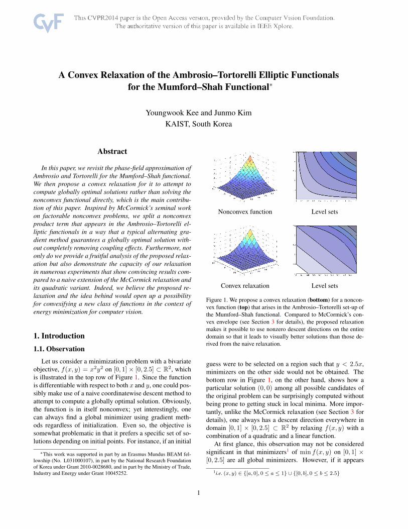
Let us consider a minimization problem with a bivariateobjective, f(x, y) = x2y2 on [0, 1] × [0, 2.5] ⊂ R2, whichis illustrated in the top row of Figure 1. Since the functionis differentiable with respect to both x and y, one could pos-sibly make use of a naive coordinatewise descent method toattempt to compute a globally optimal solution. Obviously,the function is in itself nonconvex; yet interestingly, onecan always find a global minimizer using gradient meth-ods regardless of initialization. Even so, the objective issomewhat problematic in that it prefers a specific set of so-lutions depending on initial points. For instance, if an initial

∗This work was supported in part by an Erasmus Mundus BEAM fel-lowship (No. L031000107), in part by the National Research Foundationof Korea under Grant 2010-0028680, and in part by the Ministry of Trade,Industry and Energy under Grant 10045252.

Nonconvex function Level sets

Convex relaxation Level sets

Figure 1. We propose a convex relaxation (bottom) for a noncon-vex function (top) that arises in the Ambrosio–Tortorelli set-up ofthe Mumford–Shah functional. Compared to McCormick’s con-vex envelope (see Section 3 for details), the proposed relaxationmakes it possible to use nonzero descent directions on the entiredomain so that it leads to visually better solutions than those de-rived from the naive relaxation.

guess were to be selected on a region such that y < 2.5x,minimizers on the other side would not be obtained. Thebottom row in Figure 1, on the other hand, shows how aparticular solution (0, 0) among all possible candidates ofthe original problem can be surprisingly computed withoutbeing prone to getting stuck in local minima. More impor-tantly, unlike the McCormick relaxation (see Section 3 fordetails), one always has a descent direction everywhere indomain [0, 1] × [0, 2.5] ⊂ R2 by relaxing f(x, y) with acombination of a quadratic and a linear function.

At first glance, this observation may not be consideredsignificant in that minimizers1 of min f(x, y) on [0, 1] ×[0, 2.5] are all global minimizers. However, if it appears

1i.e. (x, y) ∈ [a, 0], 0 ≤ a ≤ 1 ∪ [0, b], 0 ≤ b ≤ 2.5

1

in a combined form with another (even with a convex ob-jective), in contrast to situations where such a function isthe only objective to be minimized, one cannot be sure ofthe global optimality of a computed solution. Indeed, whenit comes to energy minimization problems in computer vi-sion, finding a globally optimal solution becomes a majoralgorithmic challenge because objectives typically consistof two or three energies—namely the data fidelity term andthe regularization term—leading to overall nonconvex ob-jectives.

In light of the observation, we consider throughoutthe paper how such a nonconvex functional that appearsin the Ambrosio–Tortorelli Γ-convergence set-up for theMumford–Shah functional can be convexified assuringnear-optimal solutions. It turns out that solutions from theproposed relaxation are energetically and visually betterthan those computed by minimizing the original nonconvexfunctional. This is the main contribution of the paper.

1.2. The Mumford–Shah Problem

Let Ω ⊂ Rn be a bounded open set and g ∈ L∞(Ω) be agiven function. The Mumford–Shah problem is given by

minu,K

α

∫Ω

|u− g|2 +

∫Ω\K|∇u|2 + βHn−1(K)

, (1)

u ∈W 1,2(Ω\K),K ⊂ Ω closed in Ω,Hn−1(K) <∞,

whereHn−1 is the (n−1)-dimensional Hausdorff measure,and α, β > 0 are fixed parameters. The functional regular-izes large sets of K, and prefers u outside the set K to beclose to g in W 1,2, namely a piecewise smooth approxima-tion of g. The functional was introduced by Mumford andShah in [21] for image segmentation (i.e., n = 2 and Ω maywell be a rectangle).

The existence of a minimizer has been proved in [12, 10]where the idea is to use a weak formulation of the prob-lem in a special class of functions of bounded variationSBV (Ω)—readers can find a complete analysis in [2]—asfollows:

minu

α

∫Ω

|u− g|2 +

∫Ω\Su

|∇u|2 + βHn−1(Su)

, (2)

where u ∈ SBV (Ω) and Su is the discontinuity set of u.Then, for any minimizer u of (2), one can recover a min-imizer of (1) by setting K = Su ∩ Ω. Since then, theMumford–Shah functional has been intensively studied, inparticular on the regularity of minimizing pairs (u,K), inapplied mathematics [20, 11] with free discontinuity prob-lems [2]. Notwithstanding the existence theorem and someresults on the regularity, exact computation of solutions forthe functional is limited to a significant extent because of itsnonconvexity. As a consequence, there has been extensive

research on efficient algorithms both in the context of con-tinuous/discrete optimization (we refer readers to [22, 17]and references therein for the continuous and discrete set-ting, respectively).

The most related work—possibly in line with the phase-field approximation of Ambrosio and Tortorelli [3] forwhich we are going to present a convex relaxation—is thosebased on the Γ-convergence set-up. That is to approximatethe functional in (2) by a sequence of regular functionals de-fined on Sobolev spaces converging to it in the sense of Γ-convergence. We will revisit the Ambrosio–Tortorelli ellip-tic functionals in Section 2; and refer readers to [5, 6, 8, 15]for different classes of approximating functionals.

In [1], Alberti et al. reformulated (2) by means of theflux of a suitable vector field going through the interfaceof the subgraph of u and provided a sufficient conditionfor minimality of some pairs of (u, Su). Unfortunately, itis still open whether there exists a divergence free vectorfield (calibration) for each minimizer of (2). Later, Pock etal. [22] proposed a fast primal-dual algorithm by relaxingthe characteristic function of the subgraph of u to [0, 1],and Strekalovskiy et al. [24] extended it to a vectorial case.However, not only is it computationally demanding to com-pute a minimizer of the relaxed problem but also it does nothold the coarea formula [14] so that global minimality is notguaranteed.

Note that we do not compare our results with those from[22] and [24] throughout the paper since our contributionis solely to convexify the Ambrosio–Tortorelli elliptic func-tionals which converge to the weak formulation (2) in thesense of Γ-convergence. In contrast, the sufficient condi-tion for minimality based on the calibration method [1] issomewhat problematic as mentioned above.

2. The Ambrosio–Tortorelli FunctionalsIn [3], Ambrosio and Tortorelli proposed a sequence

of elliptic functionals to approximate the Mumford–Shahfunctional in (2) as follows:

ATε(u, z) = α

∫Ω

|u− g|2 dx+

∫Ω

z2|∇u|2 dx

+ β

∫Ω

(ε|∇z|2 +

(z − 1)2

4ε

)dx︸ ︷︷ ︸

Lε(z)

, (3)

where ε > 0 is a fixed parameter; then ATε(u, z) is welldefined on the space

(u, z) ∈W 1,2(Ω)2 : 0 ≤ z ≤ 1

.

Here, z is a smooth edge indicator2 (i.e., z → 0 when|∇u| → ∞). Remarkably, the authors have proved thatATε(u, z) admits a minimizer and thatATε(u, z) converges

2Note that z is also called the phase-field, and Lε(z) in (3) is known asthe phase-field energy.

Input u∗ z∗

Figure 2. A pair of minimizers of the Ambrosio–Tortorelli functional. In order to compute a pair of minimizers (u∗, z∗) for theAmbrosio–Tortorelli functional, one typically resorts to an alternating optimization technique that does not guarantee a global optimalsolution due to the fact that the functional in itself is nonconvex. Yet, in practice it gives quite acceptable solutions for a number of images.

to the Mumford–Shah functional (2) as ε → 0 in the senseof Γ-convergence.

Although the Mumford–Shah functional has been nicelyapproximated by such sequence of elliptic functionals(where one can easily derive its Euler-Lagrange equationsand solve these alternatively—see Figure 2), computinga globally optimal solution is indeed a major algorithmicchallenge since (3) is still nonconvex—the second term is afunction of both u and z. In what follows, therefore, we fo-cus on the second term,

∫Ωz2|∇u|2 dx, and propose a con-

vex relaxation for it.

3. Convex RelaxationFor the sake of completeness, we start by recalling Mc-

Cormick’s seminal work on factorable nonconvex prob-lems [18]. The main result that is going to be used for thefirst relaxation for (3) is summarized as follows [19].

Theorem 1 (McCormick’s relaxation of products). Let Ω ⊂R2 be a nonempty convex set and f, f1, f2 : Ω → Rsuch that f = f1f2. Let f∪1 , f

∩1 : Ω → R be a con-

vex and concave relaxation3 of f1, respectively. Likewise,let f∪2 , f

∩2 : Ω → R be a convex and concave relaxation

of f2. Then for f1 and f2 such that L1 ≤ f1 ≤ U1 andL2 ≤ f2 ≤ U2, where L1, L2, U1, U2 ∈ R,

f∪ = maxg1 + g2 − L1L2, h1 + h2 − U1U2, (4)

where

g1 = minL2f∪1 , L2f

∩1 , g2 = minL1f

∪2 , L1f

∩2 ,

h1 = minU2f∪1 , U2f

∩1 , h2 = minU1f

∪2 , U1f

∩2 , (5)

3A convex and a concave relaxation mean f∪ ≤ f convex and f∩ ≥ fconcave on Ω, respectively.

is a convex relaxation of f .

An example Consider f = x2y2 on [0, 1] × [0, 2.5] ⊂R2, which is illustrated in Figure 3 with its level sets, then0 ≤ x2 ≤ 1 and 0 ≤ y2 ≤ 2.52. We substitute f1 and f2

with x2 and y2, respectively. By Theorem 1, their convexand concave relaxations on [0, 1] × [0, 2.5] are f∪1 = x2,f∩1 = x, f∪2 = y2, and f∩2 = 2.5y. Since g1 = 0, g2 = 0,h1 = min2.52x2, 2.52x, and h2 = miny2, 2.5y, f∪ =max0, 2.52x2 +y2−2.52; see the McCormick relaxationin Figure 3.

We now derive a similar relaxation for∫

Ωz2|∇u|2 dx

in (3), as follows.

Corollary 1 (McCormick relaxation). Let u : Ω → R beLipschitz continuous; then

FMc(u, z) :=

∫Ω

max0, L2z2 + |∇u|2 − L2 dx (6)

≤∫

Ω

z2|∇u|2 dx, (7)

where L is a Lipschitz constant for u, and FMc(u, z) is con-vex on

(W 1,2(Ω) ∩W 1,∞(Ω)

)×W 1,2(Ω).

Proof. Substitute f1 and f2 with z2 and |∇u|2, then con-sider its convex and concave relaxations: f∪1 = z2, f∩1 = z,f∪2 = |∇u|2, and f∩2 = L|∇u|, where 0 ≤ |∇u| ≤ L a.e.x in Ω by Lipschitz continuity (by Rademacher’s theorem[13]).

Let us go back to the example for a while. The convex re-laxation f∪ of f is tight in the sense of [18], yet one can seethere is no descent direction when 2.52x2 + y2 − 2.52 < 0.

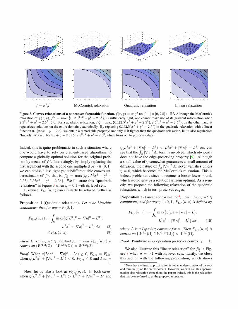
f = x2y2 McCormick relaxation Quadratic relaxation Linear relaxation

Figure 3. Convex relaxations of a nonconvex factorable function, f(x, y) = x2y2 on [0, 1]× [0, 2.5] ⊂ R2. Although the McCormickrelaxation of f(x, y), f∪ = max

0, 2.52x2 + y2 − 2.52

, is sufficiently tight, one cannot make use of its gradient information when

2.52x2 + y2 − 2.52 < 0. For a quadratic relaxation, f∪Q = max 0.1(2.52x2 + y2 − 2.52), 2.52x2 + y2 − 2.52, on the other hand, itregularizes solutions on the entire domain quadratically. By replacing 0.1(2.52x2 + y2 − 2.52) in the quadratic relaxation with a linearfunction 0.1(2.5x + y − 2.5), we obtain a remarkable property; not only is it tighter than the quadratic relaxation, but it also regularizes“linearly” when 0.1(2.5x + y − 2.5) > 2.52x2 + y2 − 2.52, which turns out to preserve edges.

Indeed, this is quite problematic in such a situation whereone would have to rely on gradient-based algorithms tocompute a globally optimal solution for the original prob-lem by means of f∪. Interestingly, by simply replacing thefirst argument with the second one multiplied by η ∈ (0, 1],we can devise a less tight yet subdifferentiable convex un-derestimator of f∪, that is, f∪Q = maxη(2.52x2 + y2 −2.52), 2.52x2 + y2 − 2.52. We illustrate this “quadraticrelaxation” in Figure 3 when η = 0.1 with its level sets.

Likewise, FMc(u, z) can similarly be relaxed further asfollows.

Proposition 1 (Quadratic relaxation). Let u be Lipschitzcontinuous; then for any η ∈ (0, 1],

FQ,η(u, z) :=

∫Ω

maxη(L2z2 + |∇u|2 − L2),

L2z2 + |∇u|2 − L2 dx (8)≤FMc(u, z), (9)

where L is a Lipschitz constant for u, and FQ,η(u, z) isconvex on

(W 1,2(Ω) ∩W 1,∞(Ω)

)×W 1,2(Ω).

Proof. When η(L2z2 + |∇u|2 − L2) ≥ 0, FQ,η = FMc;when η(L2z2 + |∇u|2 − L2) < 0, FQ,η ≤ 0 and FMc =0.

Now, let us take a look at FQ,η(u, z). In both cases,when η(L2z2 + |∇u|2 − L2) > L2z2 + |∇u|2 − L2 and

η(L2z2 + |∇u|2 − L2) < L2z2 + |∇u|2 − L2, one cansee that the

∫Ω|∇u|2 dx term is involved, which obviously

does not have the edge-preserving property [9]. Althougha small value of η somewhat guarantees a small amount ofdiffusion, the nature of

∫Ω|∇u|2 dx never vanishes unless

η = 0, which becomes the McCormick relaxation. This isindeed problematic since it becomes a looser lower bound,which would give us a solution far from optimal. As a rem-edy, we propose the following relaxation of the quadraticrelaxation, which in turn preserves edges.

Proposition 2 (Linear approximation4). Let u be Lipschitzcontinuous; and for any η ∈ (0, 1], FL,η(u, z) is defined by

FL,η(u, z) : =

∫Ω

maxη(Lz + |∇u| − L),

L2z2 + |∇u|2 − L2 dx, (10)

where L is a Lipschitz constant for u. Then FL,η(u, z) isconvex on

(W 1,2(Ω) ∩W 1,∞(Ω)

)×W 1,2(Ω).

Proof. Pointwise max operation preserves convexity.

We also illustrate this “linear relaxation” for f∪Q in Fig-ure 3 when η = 0.1 with its level sets. Lastly, we closethis section with the following proposition, which shows

4Note that the linear approximation is not an underestimator of the sec-ond term in (3) on the entire domain. However, we will call this approxi-mation also relaxation throughout the paper; indeed, this is the relaxationthat has been referred to as the proposed relaxation.

that when one of the three types of relaxations presented isplugged in the Ambrosio–Tortorelli functional (3), the over-all functional becomes a convex relaxation of the functional.

Proposition 3. Let u be Lipschitz continuous; then forevery ε > 0 and η ∈ (0, 1], a functional AT cvx

ε :(W 1,2(Ω) ∩W 1,∞(Ω)

)×W 1,2(Ω)→ R, which maps

(u, z) 7−→ α

∫Ω

|u− g|2 dx+ F (u, z) + βLε(z) (11)

is convex. Here, F (u, z) is one of the relaxations (i.e., FMc,FQ,η , and FL,η) for

∫Ωz2|∇u|2 dx.

Proof. The sum of convex functionals is convex.

3.1. Euler-Lagrange Equations

So far, we have devised such convex relaxations in away that they satisfy two properties: 1) differentiability and2) tightness. We have to admit that there is a heuristic toderive a linear relaxation from the quadratic one; that is,the quadratic relaxation has been lifted by a linear approx-imation which also maintains differentiability and convex-ity. Interestingly, it turns out that the linear relaxation hasa compelling property that comes into view, once its Euler-Lagrange equations are derived. In the following, there-fore, we derive the Euler-Lagrange equations for the re-laxations and provide complete insights—how these relax-ations work.

McCormick relaxation When L2z2 + |∇u|2 − L2 < 0,

2α(u− g) = 0, (12)β∂zLε(z) = 0; (13)

elsewhere,

2α(u− g)− div(∇u) = 0, (14)

2L2z + β∂zLε(z) = 0. (15)

As can be observed, when L2z2 + |∇u|2 − L2 < 0, thesteady-state solution is g; elsewhere, one can see there isa diffusion term div(∇u) in (14), which blurs images. In-deed, a combination of those equations makes images ex-hibit lots of speckles (salt and pepper-like noise)—see Fig-ure 5 for details.

Quadratic relaxation When η(L2z2 + |∇u|2 − L2) <L2z2+|∇u|2−L2, the corresponding Euler-Lagrange equa-tions of FQ,η(u, z) become (14) and (15); elsewhere,

2α(u− g)− η div(∇u) = 0, (16)

2ηL2z + β∂zLε(z) = 0. (17)

On either side, as can be seen, the Euler-Lagrange equa-tions contain div(∇u). Unlike the McCormick relaxation,

however, u is regularized with two different diffusion co-efficients. Here the amount of diffusion on each pixel isdecided by the max operation, which can be regarded as aninhomogeneous diffusion [25]. That is, pixels around edges(|∇u| gets larger and z gets smaller) are more likely to fallinto the region of η(|∇u|2 +L2z2−L2) < |∇u|2 +L2z2−L2 resultig in a small amount of diffusion η div(∇u) in (16)compared with div(∇u) in (14).

Linear relaxation Likewise, when η(Lz + |∇u| − L) >L2z2 + |∇u|2 − L2,

2α(u− g)− η div

(∇u|∇u|

)= 0, (18)

ηL+ β∂zLε(z) = 0. (19)

As can be seen in (18), the Euler-Lagrange equation is thesame as that of the ROF model [23]. That is, the proposedrelaxation regularizes

FL,η(u, z) = η

∫Ω

|∇u| dx+ η

∫Ω

L(z − 1) dx, (20)

when η(|∇u| + Lz − L) > |∇u|2 + L2z2 − L2. Interest-ingly, it turns out that AT cvx

ε in Proposition 3 with (10) se-lectively regularizes either

∫Ω|∇u| or

∫Ω|∇u|2 depending

on the max operation, which is similar to the Huber norm.

3.2. Vectorial Case

The (n− 1)-dimensional Hausdorff measureHn−1(Su)in (2) not only is itself very difficult to deal with; but be-comes more complicated when it is extended to a vectorialcase because one has to reasonably take into account colorcoupling among channels. On the other hand, the benefitof the Ambrosio–Tortorelli approximation is that it can bedone straightforwardly once a norm | · | for u : Ω → Rnis specified because Hn−1(Su) is well approximated byLε(z). Indeed, there are some possible (and well-studied)choices available: 1) the Frobenius norm [7], 2) the Eu-clidean norm [4], and 3) a generalization of the Jacobiandeterminant [16].

However, since those norms of a vector-valued functionhave been developed in the context of vectorial total varia-tion, meaning their dual formulations are available, metic-ulous care is required to plug them into the Ambrosio–Tortorelli functionals. For example, it has been provedin [16] that the total variation based on the Jacobian deter-minant is given by∫

Ω

J1(u)dx =

∫Ω

σ1(Du)dx, (21)

where J1 is a generalization of the Jacobian determinant,and σ1(Du) is the largest singular value of the derivativematrix. It is also mentioned that σ1(·) is not differentiable

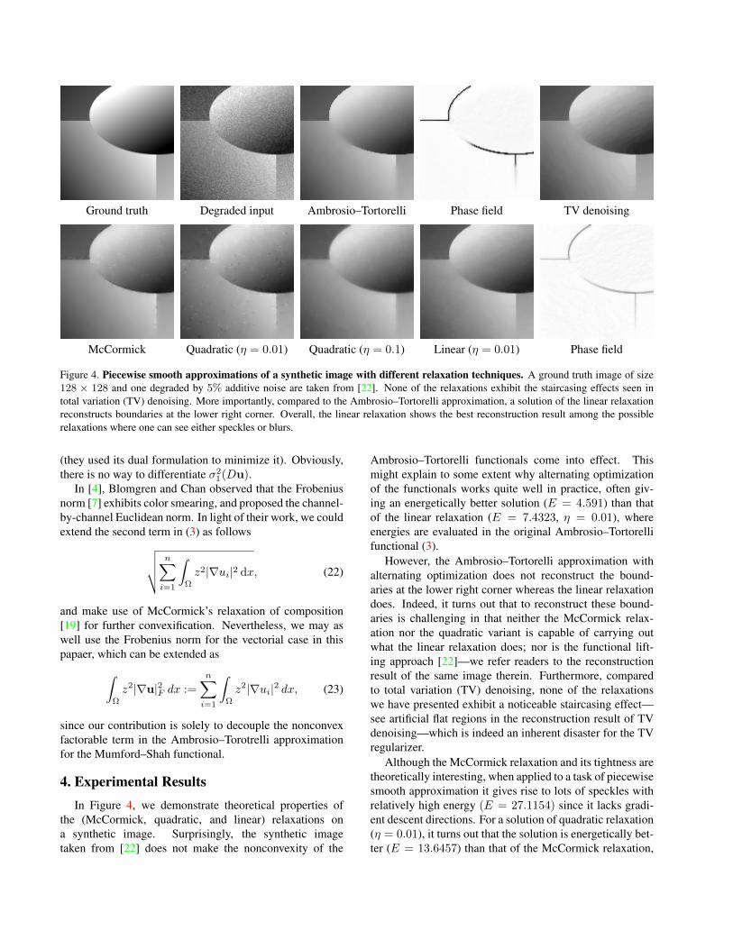
Ground truth Degraded input Ambrosio–Tortorelli Phase field TV denoising

McCormick Quadratic (η = 0.01) Quadratic (η = 0.1) Linear (η = 0.01) Phase field

Figure 4. Piecewise smooth approximations of a synthetic image with different relaxation techniques. A ground truth image of size128 × 128 and one degraded by 5% additive noise are taken from [22]. None of the relaxations exhibit the staircasing effects seen intotal variation (TV) denoising. More importantly, compared to the Ambrosio–Tortorelli approximation, a solution of the linear relaxationreconstructs boundaries at the lower right corner. Overall, the linear relaxation shows the best reconstruction result among the possiblerelaxations where one can see either speckles or blurs.

(they used its dual formulation to minimize it). Obviously,there is no way to differentiate σ2

1(Du).In [4], Blomgren and Chan observed that the Frobenius

norm [7] exhibits color smearing, and proposed the channel-by-channel Euclidean norm. In light of their work, we couldextend the second term in (3) as follows√√√√ n∑

i=1

∫Ω

z2|∇ui|2 dx, (22)

and make use of McCormick’s relaxation of composition[19] for further convexification. Nevertheless, we may aswell use the Frobenius norm for the vectorial case in thispapaer, which can be extended as∫

Ω

z2|∇u|2F dx :=

n∑i=1

∫Ω

z2|∇ui|2 dx, (23)

since our contribution is solely to decouple the nonconvexfactorable term in the Ambrosio–Torotrelli approximationfor the Mumford–Shah functional.

4. Experimental ResultsIn Figure 4, we demonstrate theoretical properties of

the (McCormick, quadratic, and linear) relaxations ona synthetic image. Surprisingly, the synthetic imagetaken from [22] does not make the nonconvexity of the

Ambrosio–Tortorelli functionals come into effect. Thismight explain to some extent why alternating optimizationof the functionals works quite well in practice, often giv-ing an energetically better solution (E = 4.591) than thatof the linear relaxation (E = 7.4323, η = 0.01), whereenergies are evaluated in the original Ambrosio–Tortorellifunctional (3).

However, the Ambrosio–Tortorelli approximation withalternating optimization does not reconstruct the bound-aries at the lower right corner whereas the linear relaxationdoes. Indeed, it turns out that to reconstruct these bound-aries is challenging in that neither the McCormick relax-ation nor the quadratic variant is capable of carrying outwhat the linear relaxation does; nor is the functional lift-ing approach [22]—we refer readers to the reconstructionresult of the same image therein. Furthermore, comparedto total variation (TV) denoising, none of the relaxationswe have presented exhibit a noticeable staircasing effect—see artificial flat regions in the reconstruction result of TVdenoising—which is indeed an inherent disaster for the TVregularizer.

Although the McCormick relaxation and its tightness aretheoretically interesting, when applied to a task of piecewisesmooth approximation it gives rise to lots of speckles withrelatively high energy (E = 27.1154) since it lacks gradi-ent descent directions. For a solution of quadratic relaxation(η = 0.01), it turns out that the solution is energetically bet-ter (E = 13.6457) than that of the McCormick relaxation,

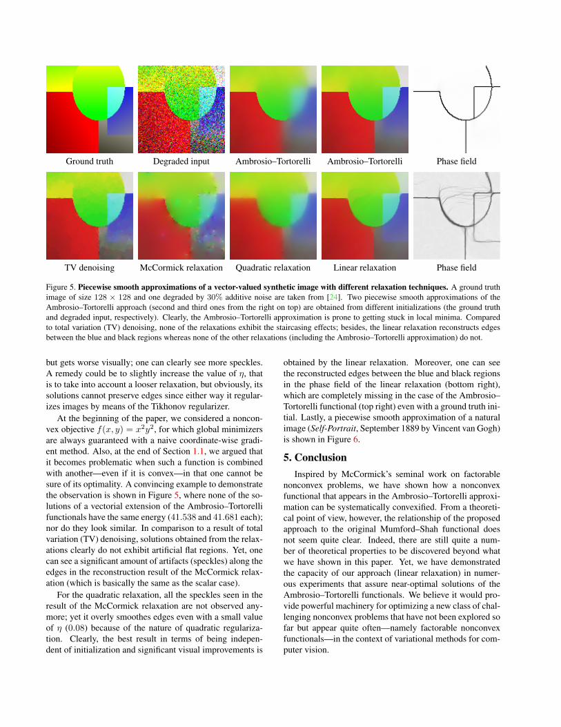
Ground truth Degraded input Ambrosio–Tortorelli Ambrosio–Tortorelli Phase field

TV denoising McCormick relaxation Quadratic relaxation Linear relaxation Phase field

Figure 5. Piecewise smooth approximations of a vector-valued synthetic image with different relaxation techniques. A ground truthimage of size 128 × 128 and one degraded by 30% additive noise are taken from [24]. Two piecewise smooth approximations of theAmbrosio–Tortorelli approach (second and third ones from the right on top) are obtained from different initializations (the ground truthand degraded input, respectively). Clearly, the Ambrosio–Tortorelli approximation is prone to getting stuck in local minima. Comparedto total variation (TV) denoising, none of the relaxations exhibit the staircasing effects; besides, the linear relaxation reconstructs edgesbetween the blue and black regions whereas none of the other relaxations (including the Ambrosio–Tortorelli approximation) do not.

but gets worse visually; one can clearly see more speckles.A remedy could be to slightly increase the value of η, thatis to take into account a looser relaxation, but obviously, itssolutions cannot preserve edges since either way it regular-izes images by means of the Tikhonov regularizer.

At the beginning of the paper, we considered a noncon-vex objective f(x, y) = x2y2, for which global minimizersare always guaranteed with a naive coordinate-wise gradi-ent method. Also, at the end of Section 1.1, we argued thatit becomes problematic when such a function is combinedwith another—even if it is convex—in that one cannot besure of its optimality. A convincing example to demonstratethe observation is shown in Figure 5, where none of the so-lutions of a vectorial extension of the Ambrosio–Tortorellifunctionals have the same energy (41.538 and 41.681 each);nor do they look similar. In comparison to a result of totalvariation (TV) denoising, solutions obtained from the relax-ations clearly do not exhibit artificial flat regions. Yet, onecan see a significant amount of artifacts (speckles) along theedges in the reconstruction result of the McCormick relax-ation (which is basically the same as the scalar case).

For the quadratic relaxation, all the speckles seen in theresult of the McCormick relaxation are not observed any-more; yet it overly smoothes edges even with a small valueof η (0.08) because of the nature of quadratic regulariza-tion. Clearly, the best result in terms of being indepen-dent of initialization and significant visual improvements is

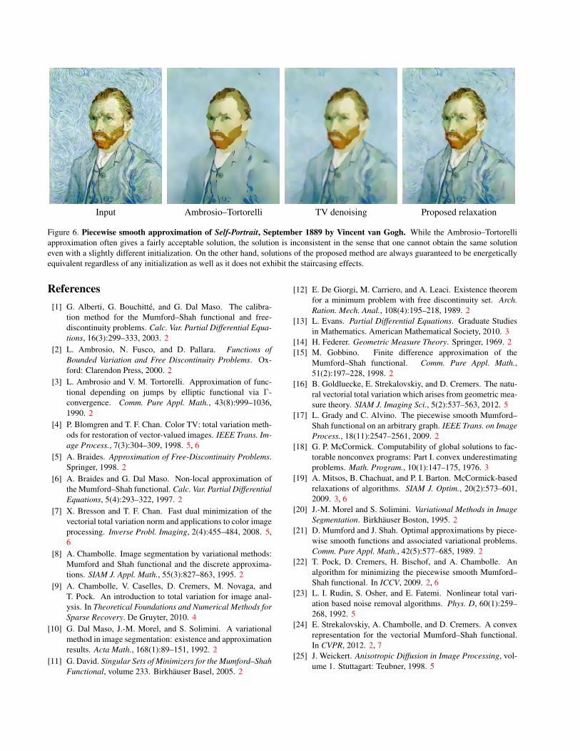
obtained by the linear relaxation. Moreover, one can seethe reconstructed edges between the blue and black regionsin the phase field of the linear relaxation (bottom right),which are completely missing in the case of the Ambrosio–Tortorelli functional (top right) even with a ground truth ini-tial. Lastly, a piecewise smooth approximation of a naturalimage (Self-Portrait, September 1889 by Vincent van Gogh)is shown in Figure 6.

5. ConclusionInspired by McCormick’s seminal work on factorable

nonconvex problems, we have shown how a nonconvexfunctional that appears in the Ambrosio–Tortorelli approxi-mation can be systematically convexified. From a theoreti-cal point of view, however, the relationship of the proposedapproach to the original Mumford–Shah functional doesnot seem quite clear. Indeed, there are still quite a num-ber of theoretical properties to be discovered beyond whatwe have shown in this paper. Yet, we have demonstratedthe capacity of our approach (linear relaxation) in numer-ous experiments that assure near-optimal solutions of theAmbrosio–Tortorelli functionals. We believe it would pro-vide powerful machinery for optimizing a new class of chal-lenging nonconvex problems that have not been explored sofar but appear quite often—namely factorable nonconvexfunctionals—in the context of variational methods for com-puter vision.

Input Ambrosio–Tortorelli TV denoising Proposed relaxation

Figure 6. Piecewise smooth approximation of Self-Portrait, September 1889 by Vincent van Gogh. While the Ambrosio–Tortorelliapproximation often gives a fairly acceptable solution, the solution is inconsistent in the sense that one cannot obtain the same solutioneven with a slightly different initialization. On the other hand, solutions of the proposed method are always guaranteed to be energeticallyequivalent regardless of any initialization as well as it does not exhibit the staircasing effects.

References[1] G. Alberti, G. Bouchitte, and G. Dal Maso. The calibra-

tion method for the Mumford–Shah functional and free-discontinuity problems. Calc. Var. Partial Differential Equa-tions, 16(3):299–333, 2003. 2

[2] L. Ambrosio, N. Fusco, and D. Pallara. Functions ofBounded Variation and Free Discontinuity Problems. Ox-ford: Clarendon Press, 2000. 2

[3] L. Ambrosio and V. M. Tortorelli. Approximation of func-tional depending on jumps by elliptic functional via Γ-convergence. Comm. Pure Appl. Math., 43(8):999–1036,1990. 2

[4] P. Blomgren and T. F. Chan. Color TV: total variation meth-ods for restoration of vector-valued images. IEEE Trans. Im-age Process., 7(3):304–309, 1998. 5, 6

[5] A. Braides. Approximation of Free-Discontinuity Problems.Springer, 1998. 2

[6] A. Braides and G. Dal Maso. Non-local approximation ofthe Mumford–Shah functional. Calc. Var. Partial DifferentialEquations, 5(4):293–322, 1997. 2

[7] X. Bresson and T. F. Chan. Fast dual minimization of thevectorial total variation norm and applications to color imageprocessing. Inverse Probl. Imaging, 2(4):455–484, 2008. 5,6

[8] A. Chambolle. Image segmentation by variational methods:Mumford and Shah functional and the discrete approxima-tions. SIAM J. Appl. Math., 55(3):827–863, 1995. 2

[9] A. Chambolle, V. Caselles, D. Cremers, M. Novaga, andT. Pock. An introduction to total variation for image anal-ysis. In Theoretical Foundations and Numerical Methods forSparse Recovery. De Gruyter, 2010. 4

[10] G. Dal Maso, J.-M. Morel, and S. Solimini. A variationalmethod in image segmentation: existence and approximationresults. Acta Math., 168(1):89–151, 1992. 2

[11] G. David. Singular Sets of Minimizers for the Mumford–ShahFunctional, volume 233. Birkhauser Basel, 2005. 2

[12] E. De Giorgi, M. Carriero, and A. Leaci. Existence theoremfor a minimum problem with free discontinuity set. Arch.Ration. Mech. Anal., 108(4):195–218, 1989. 2

[13] L. Evans. Partial Differential Equations. Graduate Studiesin Mathematics. American Mathematical Society, 2010. 3

[14] H. Federer. Geometric Measure Theory. Springer, 1969. 2[15] M. Gobbino. Finite difference approximation of the

Mumford–Shah functional. Comm. Pure Appl. Math.,51(2):197–228, 1998. 2

[16] B. Goldluecke, E. Strekalovskiy, and D. Cremers. The natu-ral vectorial total variation which arises from geometric mea-sure theory. SIAM J. Imaging Sci., 5(2):537–563, 2012. 5

[17] L. Grady and C. Alvino. The piecewise smooth Mumford–Shah functional on an arbitrary graph. IEEE Trans. on ImageProcess., 18(11):2547–2561, 2009. 2

[18] G. P. McCormick. Computability of global solutions to fac-torable nonconvex programs: Part I. convex underestimatingproblems. Math. Program., 10(1):147–175, 1976. 3

[19] A. Mitsos, B. Chachuat, and P. I. Barton. McCormick-basedrelaxations of algorithms. SIAM J. Optim., 20(2):573–601,2009. 3, 6

[20] J.-M. Morel and S. Solimini. Variational Methods in ImageSegmentation. Birkhauser Boston, 1995. 2

[21] D. Mumford and J. Shah. Optimal approximations by piece-wise smooth functions and associated variational problems.Comm. Pure Appl. Math., 42(5):577–685, 1989. 2

[22] T. Pock, D. Cremers, H. Bischof, and A. Chambolle. Analgorithm for minimizing the piecewise smooth Mumford–Shah functional. In ICCV, 2009. 2, 6

[23] L. I. Rudin, S. Osher, and E. Fatemi. Nonlinear total vari-ation based noise removal algorithms. Phys. D, 60(1):259–268, 1992. 5

[24] E. Strekalovskiy, A. Chambolle, and D. Cremers. A convexrepresentation for the vectorial Mumford–Shah functional.In CVPR, 2012. 2, 7

[25] J. Weickert. Anisotropic Diffusion in Image Processing, vol-ume 1. Stuttagart: Teubner, 1998. 5