A Correspondence Between the Isobaric Ring and

Multiplicative Arithmetic Functions

Trueman MacHenry and Kieh Wong

November 20, 2009

ABSTRACT

We give a representation of the classical theory of multiplicative arithmetic functions (MF) inthe ring of symmetric polynomials written on the isobaric basis. The representing elements arerecursive sequences of Schur-hook polynomials evaluated on subrings of the complex numbers. Themultiplicative arithmetic functions are units in the Dirichlet ring of arithmetic functions, and theirproperties can be described locally, that is, at each prime number p. Our representation is, hence, alocal representation. This representation enables us to clarify and generalize classical results, e.g.,the Busche-Ramanujan identity, as well as to give a richer structural description of the convolutiongroup of multiplicative functions. It is a consequence of the representation that the MFs can bedefined in a natural way on the negative powers of the prime p which, in turn, leads to a naturalextension of Schur-hook polynomials to negatively indexed Schur-hook polynomials.

CONTENTS0. Introduction1. Ring of Isobaric Polynomials2. The Companion Matrix and Core Polynomials3 The Ring of Arithmetic Functions4. Relation Between Arithmetic Functions and the WIP-Module5. Examples6. Specially Multiplicative Arithmetic Functions7. Structure of the Convolution Group of Multiplicative Arithmetic Functions Reconsidered8. Norms

0. INTRODUCTION

In this paper we give a representation of the classical theory of multiplicative arithmetic functions(MF) in the ring of symmetric polynomials. The Dirichlet ring of arithmetic functions A∗ iswell known to be a unique factorization domain.(see Cashwell and Everett [?]). Its ring theoreticproperties have been investigated in, e.g., Rearick [?] and [?], Shapiro [?], Carroll and Gioia [?],MacHenry [?], MacHenry and Tudose [?]. The multiplicative arithmetic functions are units inthis ring and their properties can be described locally, that is, at each prime number p, (see, e.g.,McCarthy [?], Sivaramakishnan[?] and Vaidyanathswamy, [?]). It is this local behaviour which wetake advantage of to construct a representation in terms of a certain class of symmetric polynomials

1

called weighted isobaric polynomials [?]. It is advantageous to use the isobaric basis as a basis forthe ring of symmetric polynomials; we describe this basis in Section 1. Henceforth, we refer to thesymmetric polynomials in this basis as the ring of isobaric polynomials.

The link between the theory of symmetric polynomials and the theory of multiplicative, arith-metic functions is that of linear recurrence, especially the ideas contained in MacHenry and Wong[?]; (also see Rutkowski [?], Lascoux [?] and Hou and Mu [?]). The isobaric ring contains a cer-tain submodule, the submodule of weighted isobaric polynomials (WIP), which is generated as aZ-module by the Schur-hook polynomials. This module has the property that it can be parti-tioned into sequences which are linear recursions (see [?]). It contains the sequence of GeneralizedFibonacci Polynomials (GFP), and the sequence of Generalized Lucas Polynomials (GLP), (seeMacHenry [?]). It turns out that each of these sequences, when the indeterminates are evaluatedover a subring of the complex numbers, is the evaluation of a local sequence of multiplicative func-tions, i.e., a multiplicative function at a prime p. Moreover, every MF is represented locally by suchsequences; in fact, the GFP-sequence is sufficient for this purpose. This fact brings the machineryof the isobaric ring to bear with respect to the convolution group of multiplicative functions. Theimportance of linear recursions in the theory of MF is recognized in Laohakosol and Pabhapote[?] and in Rutkowski [?]; however, the connection between multiplicative functions and symmet-ric functions and the power of the isobaric notation to simplify and reveal basic facts about thestructure of MF is not made explicit in these papers.

The same machinery of linear recurrences in the isobaric setting was used in MacHenry andWong [?] to study number fields. A consequence of the results in that paper implies a certainstrong connection between the structure of number fields, the algebraic structure of multiplicativefunctions, and periodicity in the theory of recursion. The connection between A∗ and the symmetricpolynomials was exploited in [?] and in [?]. In the first of these papers it was used to prove thatthe group of multiplicative functions generated by the completely multiplicative functions is freeabelian. In the second paper, a constructive procedure using isobaric polynomials was given forembedding this group into its divisible closure (also see [?]).

In Section 1, we define the weighted isobaric polynomials (WIP’s) and give a formula for themindependent of recursion.

In Section 2, the notion of the core polynomial is introduced and the infinite companion ma-trix and its properties are described, (see also [?], Lascoux [?]). This infinite matrix extends theWIP-sequences in the negative direction, that is, provides negatively-indexed functions as well aspositively-indexed ones. Negatively indexed sequences of isobaric polynomials induce, using thelinear recursion property, negatively indexed MFs. Also, in this section generating functions areprovided for the isobaric polynomials (and their MF counterparts).

In Section 3, we discuss the ring of arithmetic functions and introduce an important classificationscheme for them.

In Section 4, the main theorem, the Correspondence Theorem (Theorem 1) asserting the relationbetween multiplicative arithmetic functions and the WIP-module is proved.

Given a prime p, let χ ∈ M with local core C(X), k finite or infinite, and let Fk(t) be thesequence of GFP’s induced by this core, then

Fk,n(t) = χ(pn)

In this section it is shown that for each MF α, not only do we have its local representationin terms of GFP’s, but in addition, each column of the infinite companion matrix also determines

2

an MF. Each element in any column of A∞ is a Schur-hook polynomial. (The negatively indexedone’s provide an extension of the idea of Schur polynomials.) All of these Schur polynomials, thenegatively-indexed ones as well as the positively-indexed ones, can be conveniently computed usingJacobi-Trudi formulae in their isobaric form.

In Section 5, we give a collection of examples showing the details of the application of thecorrespondence theorem .

In Section 6, we look at the theory of specially multiplicative arithmetic functions, the theoremof McCarthy and the Busche-Ramanujan identity from the point of view of isobaric representation,putting these ideas in a different and more transparent light. In particular we show that thespecially multiplicative arithmetic functions are not so special after all; the theorem of McCarthyis a trivially redundant assertion that specially multiplicative functions are quadratic ([?], theorem1.12, especially part (4)). Thus the recursion formula for multiplicative functions is a generalizationof the McCarthy theorem. In the case of Busche-Ramanujan, we give a generalization and aninterpretation. In the language of this paper, the (Busche-Ramanujan) theorem (see [?] and [?])becomes Proposition?? which states that when a multiplicative function is represented by the GFPF , then

(4.1) F2,r+s = F2,rF2,s + t2F2,r−1F2,s−1

(4.2) F2,rF2,s = F2,r+s − t2F2,r+s−2 + ...+ (−t2)jF2,r+s−2j + ...+ (−t2)rF2,s−r

where the degree of the core is 2, and j = 1, ..., r.

In Section 7, the notions of type and valence are introduced Type is a classification of thelocal convolution group of multiplicative arithmetic functions in terms of ranges and domains of itselements. There are four types

(fin, fin), (inf, fin), (fin, inf), and(inf, inf),

where for example (fin, inf) means that the domain contains only finitely many non-zero elements,and the range contains infinitely many non-zero elements. Here we show, e.g., that all of these typesexist and are mutually exclusive, and that type 1 has only a single representative, the identityfunction.

Valence is also an ordered pair, namely, a pair (r, s), where r is the number of degree one factorsin a mulitplicative function χ and s is the number of inverses of degree 1 factors in χ, where χ iswritten in reduced form.

We also show how a theorem of Laohakosol and Pabhapote [?] extending Busche-Ramanujanidentities to multiplicative functions of mixed type can be simplified and clarified.

In Section 8, we propose a classification system for MF which consists of the categories degree,type, and valence, which enables us to take a refined look at the structure of MF’s. The degree isthe degree of the core polynomial, the type of an MF, as mentioned above, has to do with the sizesof its domain and range, and the valence, with its convolution structure. We discuss and extendsome results of Laohakosol-Pabhapote, [?], Proposition ??, Theorem ?? and especially, Theorem?? which gives a candidate for a generalization of the Busche-Ramanujan identity in terms ofSchur-hook functions.

In Section 9, we discuss the Kesava Menon Norm for MF in terms of the framework of this

3

paper, showing that it is multiplicative and preserves degree. This is what the Kesava Menon normlooks like in isobaric terminology:

N (Fn) =2n∑j=0

(−1)jF2n−jFj

or, equivalently

N (Fn) = (2n−1∑j=0

(−1)jF2n−jFj) + (−1)nF 2n

In this section, we prove the multiplicitive property of the Kesava Menon norm, that is that theKesava Menon norm preserves convolution products, in the framework of this paper.

The authors would like to thank an anonymous referee for many useful suggestions, both stylisticand mathematical, which are responsible for important improvements in this paper.

1. RING OF ISOBARIC POLYNOMIALS.

Definition 1 For a fixed k, an isobaric polynomial is a polynomial of the form

Pk,n(t1, ..., tk) =∑α`n

Cαtα11 ...tαk

k , α = (α1, ..., αk),∑

jαj = n, αj ∈ N

The condition∑jα = n is equivalent to: (1α1 , ..., kαk) is a partition of n, whose largest part is

at most k, and we write this in the abbreviated, and somewhat unorthodox form, as α ` n. (Notethat, given k the vector αi is sufficient information for reconstructing the partition.) Thus anisobaric polynomial of isobaric degree n is a polynomial whose monomials represent partitions of nwith largest part not exceeding k. These polynomials form a graded commutative ring with identityunder ordinary multiplication and addition of polynomials, graded by isobaric degree. This ring isnaturally isomorphic to the ring of symmetric polynomials, where the isomorphism is given by theinvolution Ω:

tj (−1)j+1ej

with ej being the j-th elementary symmetric polynomial in the k−th gradation of the graded ring ofsymmetric polynomials on the monomial basis, (see [?] and [?]). For example, if k = 2 and λ1, λ2is the monomial basis, then for j = 1, e1 = λ1 + λ2 and for j = 2 e2 = −λ1λ2 This isomorphismassociates the Complete Symmetric Polynomials (CSP) in the monomial ring with the GeneralizedFibonacci Polynomials (GFP) in the isobaric ring. It also associates the Power Symmetric Poly-nomials (PSP) with the Generalized Lucas Polynomials (GLP) in the isobaric ring, (see [?], andMacdonald [?]) . We denote these two sequences of polynomials, respectively, Fk,n and Gk,nwhere k is the number of variables, and n is the isobaric degree. The correspondence between (CSP)and (GFP) and the correspondence between (PSP) and (GLP) can be shown inductively using thefact that (GFP) and (GLP) are linearly recursions of degree k; that is,

Fk,n = t1Fk,n−1 + t2Fk,n−2 + ...+ tkFn−k

4

andGk,n = t1Gk,n−1 + t2Gk,n−2 + ...+ tkGn−k

with initial conditions given by,

Fk,0 = 1, Fk,−1 = 0, ..., Fk,−k+1 = 0

andGk,0 = k,Gk,−1 = 0, ..., Gk,−k+1 = 0.

In Section 2 we show that this choice of initial conditions arises in a natural way..The (GFP) and (GLP) can be explicitly represented as follows:

Fk,n =∑α`n

(|α|

α1...αk

)tα11 ...tαk

k ,

Gk,n =∑α`n

(|α|

α1...αk

)n

|α|tα11 ...tαk

k ,

where |α| =∑αj , j = 1 + 2 + ...+ k.

Note that when k = 2 and t1 = 1, t2 = 1, F2,n(1, 1) and G2,n(1, 1) are, respectively, the sequenceof Fibonacci numbers and the sequence of Lucas numbers. On the other hand, for a fixed k boththe GFP and the GLP are linearly recursive sequences indexed by n, and as we shall see below, theindexing can be extended to the negative integers with preservation of the linear recursion property(see [?], and [?]). All other recursive sequences of isobaric polynomials are linear combinations ofisobaric reflects of sequences of Schur-hook polynomials (to be explicitly defined in Section 2) andform a (free) Z-module, the module of Weighted Isobaric Polynomials (WIP) (see [?]and [?]). Itis a remarkable fact that the only isobaric polynomials that can be elements in linearly recursivesequences of isobaric polynomials are those that occur in one of the sequences in the WIP-module([?], Theorem 3.4) . Every sequence in the WIP-module can be presented in a closed form whosestructure explains the term weighted.

Pω,k,n =∑α`n

(|α|

α1, ..., αk

) ∑αjωj∑αj

tα11 ...tαk

k .

ω = (ω1, ..., ωk)

where ω = (ω1, ..., ωk) is the weight vector, usually taken to be an integer vector. k and ω arefixed and n varies. Both the GFP’s and the GLP’s are weighted sequences, the weighting beinggiven by, respectively, (1, 1, ..., 1, ...) for the GFPs, and (1, 2, ..., j, ...) for the GLPs. The Schur-hook polynomial sequences, i.e., the columns of the infinite companion matrix (see Section 2) haveweightings of the form (1, 1, ..., 1, ...) or ±(0, ..., 1, ..., 1, ...), that is, 0 up to k − 1 zeros as theirleading coordinates and 1′s elsewhere . The GLPs are alternating sums of all of the Schur-hooksof the same isobaric degree (see [?], [?] and [?]).

Moreover, it is important to note that a new variable tk will appear in a WIP polynomial Pω,k,nfor the first time when n = k. Thus, for fixed ω and k the Pω,k,jare the same for all |j| < k. Wecall this the conservation principle. We illustrate this with a listing of the first five GFPs, takingthe point of view that k varies as n varies.

5

• Fk,1 = t1

• Fk,2 = t21 + t2

• Fk,3 = t31 + 2t1t2 + t3

• Fk,4 = t41 + 3t21t2 + t22 + 2t1t3 + t4

• Fk,5 = t51 + 4t31t2 + 3t1t22 + 3t21t3 + 2t2t3 + 2t1t4 + t5

We need another concept which binds these various sequences together, namely, that of the corepolynomial.

Definition 2 Given a set of variables t = (t1, ..., tk), the core polynomial is the polynomial

[t1, ..., tk] = Xk − t1Xk−1 − ...− tk.

This polynomial is related to the various sequences of isobaric polynomials by the two fun-damental theorems of symmetric functions, the first being that the ring of symmetric functionsis generated by the elementary symmetric functions, the second, that the coefficients of a monicpolynomial are (up to signs) elementary symmetric functions of the roots. A rather striking way ofimmediately achieving this connection is through the companion matrix (CM).

2. THE COMPANION MATRIX AND CORE POLYNOMIALS

Given the core polynomial, [t1, ..., tk], the companion matrix is the matrix

A =

0 1 0 ... 00 0 1 ... 0... ... ... ... ...0 0 0 ... 1tk tk−1 tk−2 ... t1

.

A useful property of the companion matrix A is that when A operates on An by multiplicationon the left, say, the result is that all of the rows of An are shifted up one row, the first rowdisappears, and the new last row is the result of A operating on the last row of An. The upshot is,of course, An+1. We can make use of this fact by making the following construction. Starting withthe k× k−matrix A, we construct a k× (k+ 1)−matrix whose last row is the result of A operatingon the right on the last row vector of A. We repeat this process on the k × (k + 1)−matrix justconstructed. And so on. The limit of this process is a k×∞−matrix whose k×k−contiguous blocksconstitute the orbit of A operating on itself repeatedly. These blocks are the positive powers of A. IfA is non-singular, an analogous process, starting with A using A−1 as the operator, produces a newtop row each time whose k × k−contiguous blocks are the negative powers of A. This produces adoubly-infinite (top and bottom) matrix with k columns, which we denote A∞, and call the infinitecompanion matrix.(see [?] and Chen and Louck [?]). We write the orbit matrix A∞ described aboveas follows:

6

A∞ =

... ... ... ...(−1)k−1S(−2,1k−1) ... −S(−2,1) S(−2)

(−1)k−1S(−1,1k−1) ... −S(−1,1) S(−1)

(−1)k−1S(0,1k−1) ... −S(0,1) S(0)

(−1)k−1S(1,1[k−1) ... −S(1,1) S(1)

(−1)k−1S(2,1k−1) ... −S(2,1) S(2)

(−1)k−1S(3,1k−1) ... −S(3,1) S(3)

(−1)k−1S(4,1k−1) ... −S(4,1) S(4)

... ... ...

= ((−1)k−jS(n,1k−j))k×∞

Here is a typical k × k− block in A∞ when k = 3:

An =

S(n−2,12) −S(n−2,1) S(n−2)

S(n−1,12) −S(n−1,1) S(n−1)

S(n,12) −S(n,1) S(n)

Note that

S(n−2) = F3,n−2, S(n−1) = F3,n−1, S(n) = F3,n

This matrix can be regarded as recording all of the elements of the free-abelian group (an infinitecyclic group) generated by the matrix A. An is specifically the k×k−block whose lower right handelement in the representation above is denoted S(n) = Fk,n, n ∈ Z. It turns out that the entriesin this matrix are the positive and negatively-indexed Schur-hook polynomials induced by Youngdiagrams of arm-length n and leg-length k − j (see [?], page 2 for this terminology) but appear inthis matrix in their isobaric form (what has been called in previous papers, isobaric reflects (see [?]and [?])). However, the idea of having the indexing range over the negative integers appears to benew. So we shall describe how the Jacobi-Trudi formula (see [?, ?]) can be used to produce isobaricpolynomials in both the well-known case of non-negative indices as well as in the newly introducednegatively indexed case.

Let (θ1, θ2, ..., θr) be a partition of n (∑θi = n), listed in weakly descending order (the partition

(1α1 , 2α2 , ..., kαk) written in this fashion would be (k, ..., k, ..., 2, ..., 2, 1, ...1), each j written αj times;thus

∑jαj = n. Then the Jacoby-Trudi formula for the Schur polynomial on the isobaric basis

induced by this partition is given by the determinant of the |α| × |α|−matrix, where |α| =∑αi.

S(θ1, θ2, ..., θk) = det(Fθi−i+j).

It is straightforward to check that this is consistent with first computing the Schur functions on themonomial basis and then going to the isobaric basis by way of the mapping tj → (−1)j+1ej above.It is also straightforward to show that when the Schur polynomials are hook-polynomials, this isconsistent with extending the sequences to the negatively indexed polynomials by linear recursion.Perhaps an example would be useful. Consider the Schur-hook polynomial denoted by S(2,12), apolynomial of isobaric degree 4.

S(2,12) = det

F2 F3 F4

F0 F1 F2

0 F0 F1

7

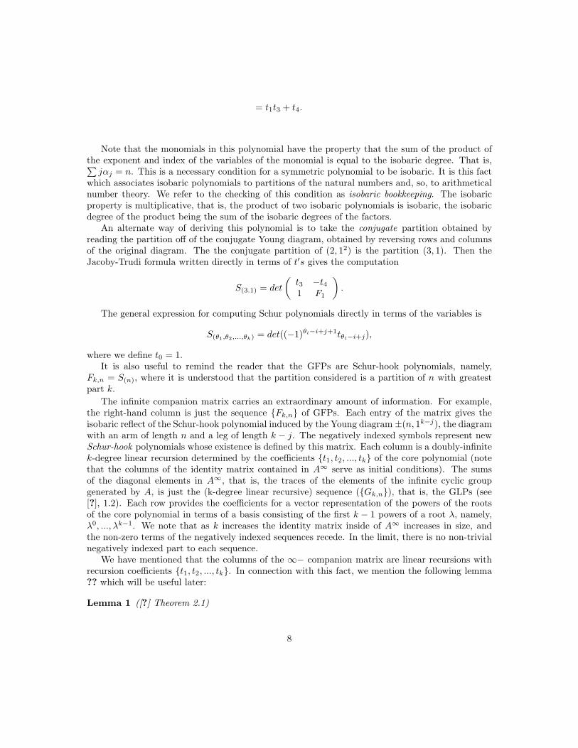
= t1t3 + t4.

Note that the monomials in this polynomial have the property that the sum of the product ofthe exponent and index of the variables of the monomial is equal to the isobaric degree. That is,∑jαj = n. This is a necessary condition for a symmetric polynomial to be isobaric. It is this fact

which associates isobaric polynomials to partitions of the natural numbers and, so, to arithmeticalnumber theory. We refer to the checking of this condition as isobaric bookkeeping. The isobaricproperty is multiplicative, that is, the product of two isobaric polynomials is isobaric, the isobaricdegree of the product being the sum of the isobaric degrees of the factors.

An alternate way of deriving this polynomial is to take the conjugate partition obtained byreading the partition off of the conjugate Young diagram, obtained by reversing rows and columnsof the original diagram. The the conjugate partition of (2, 12) is the partition (3, 1). Then theJacoby-Trudi formula written directly in terms of t′s gives the computation

S(3.1) = det

(t3 −t41 F1

).

The general expression for computing Schur polynomials directly in terms of the variables is

S(θ1,θ2,...,θk) = det((−1)θi−i+j+1tθi−i+j),

where we define t0 = 1.It is also useful to remind the reader that the GFPs are Schur-hook polynomials, namely,

Fk,n = S(n), where it is understood that the partition considered is a partition of n with greatestpart k.

The infinite companion matrix carries an extraordinary amount of information. For example,the right-hand column is just the sequence Fk,n of GFPs. Each entry of the matrix gives theisobaric reflect of the Schur-hook polynomial induced by the Young diagram ±(n, 1k−j), the diagramwith an arm of length n and a leg of length k − j. The negatively indexed symbols represent newSchur-hook polynomials whose existence is defined by this matrix. Each column is a doubly-infinitek-degree linear recursion determined by the coefficients t1, t2, ..., tk of the core polynomial (notethat the columns of the identity matrix contained in A∞ serve as initial conditions). The sumsof the diagonal elements in A∞, that is, the traces of the elements of the infinite cyclic groupgenerated by A, is just the (k-degree linear recursive) sequence (Gk,n), that is, the GLPs (see[?], 1.2). Each row provides the coefficients for a vector representation of the powers of the rootsof the core polynomial in terms of a basis consisting of the first k − 1 powers of a root λ, namely,λ0, ..., λk−1. We note that as k increases the identity matrix inside of A∞ increases in size, andthe non-zero terms of the negatively indexed sequences recede. In the limit, there is no non-trivialnegatively indexed part to each sequence.

We have mentioned that the columns of the ∞− companion matrix are linear recursions withrecursion coefficients t1, t2, ..., tk. In connection with this fact, we mention the following lemma?? which will be useful later:

Lemma 1 ([?] Theorem 2.1)

8

A linear recursion is periodic if and only if every root of the core polynomial is a complex rootof unity. In particular, if the core polynomial is the cyclotomic polynomial CP (n) of degree ϕ(n),where ϕ is the Euler totient function, then its associated linear recursion is periodic with period n(see[16])

On the other hand, every linear recursion is periodic modulo the prime (p) for every rationalprime p. The p-period of a linear recursion induced by [t1, ..., tk] satisfies cp[t] 6 pk − 1 [?].

Finally, we remark that while the positively indexed Schur-hook polynomials are induced bypartitions of the form (1r, n), n positive, it is consistent with the notation to regard the negativelyindexed Schur-hooks as induced by the ”signed” partition (1r, n) in the sense of George E. Andrews,(see[?]).

There are other algebraic structures that can be imposed on the isobaric ring, (see [?]). Forsubsequent use, we want to consider one such, a new product on the elements of the WIP-module,namely, the convolution product.

Definition 3 For a fixed k, the convolution product of two elements Un and Vn in the WIP-moduleis the convolution Un ∗ Vn =

∑nj=0 UjVn−j, where Un and Vn are n−th terms in the WIP-module.

Remark 1 Taking the convolution product of tn and, say Fn, we are regarding tn as the sequencetjn0 . For example, linear recursion given by Fn − t1Fn−1 − ... − tkFk is just Fn ∗ −tn. Observealso that the tj = (−1)n−1S(1,1n−1) is an entry in A∞.

It turns out that this gives a graded group structure to the WIP-module. In particular, −tn isthe convolution inverse of Fk,n, where tj = 0 when j > k and t0 = 1 (recall that −tj , j = 0...., k arethe coefficients of the core polynomial). The fact that this is the convolution inverse is a consequenceof the statement that Fk,n =

∑kj=1 tjFk−j , that is, that the GFP-sequence is a k-th order linear

recurrence.We have regarded the t′js as indeterminates so far, and the core polynomial as a generic kth-

degree polynomial. That is, we have been operating with polynomials, not polynomial functions;but there are many applications in which it is convenient to evaluate these polynomials over asuitable ring. It is in this context that the names Generalized Fibonacci and Generalized Lucaswere chosen. As was pointed out in Section 1 above, if k = 2 and t1 = 1 = t2, then a GFP isjust the Fibonacci sequence, and a GLP is the Lucas Sequence. Taking this point of view, it iseasy to show that every linearly recursive numerical sequence is contained as a sequence in theWIP-module.

For some purposes, we shall want to choose the evaluation ring to be Z, but other rings will alsobe useful.

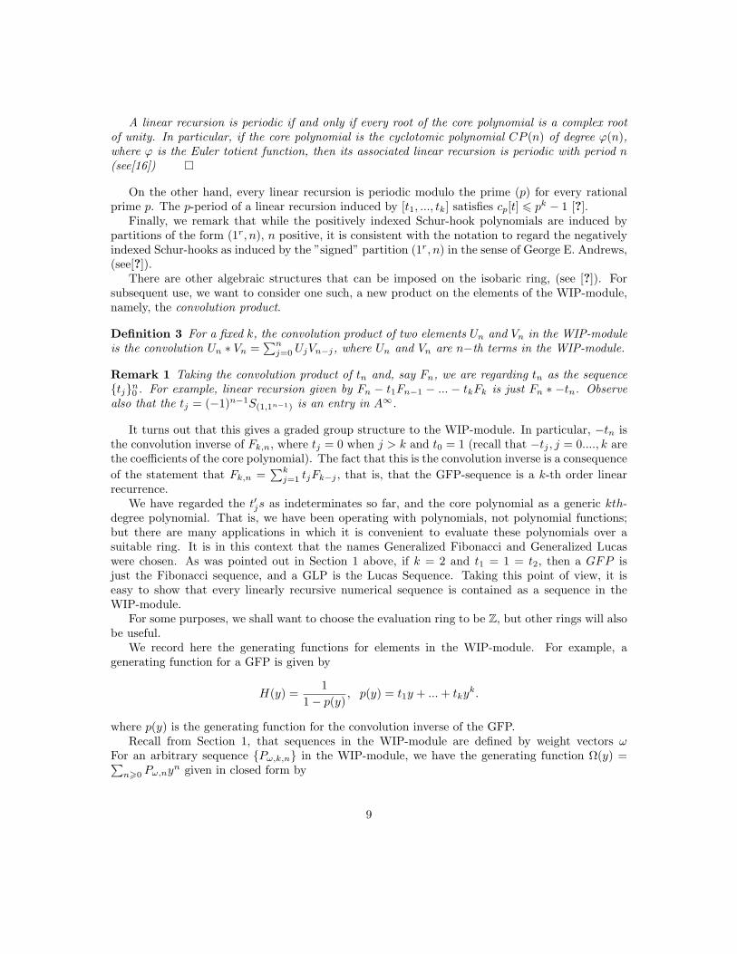
We record here the generating functions for elements in the WIP-module. For example, agenerating function for a GFP is given by

H(y) =1

1− p(y), p(y) = t1y + ...+ tky

k.

where p(y) is the generating function for the convolution inverse of the GFP.Recall from Section 1, that sequences in the WIP-module are defined by weight vectors ω

For an arbitrary sequence Pω,k,n in the WIP-module, we have the generating function Ω(y) =∑n>0 Pω,ny

n given in closed form by

9

Proposition 1

Ω(y) = 1 +ω1t1y + ω2t2y

2 + ...+ ωktkyk

1− p(y)

where Pω,0 = 1,

(see [?]).In [?] we studied the sequences in the WIP-module with respect to periodicity and periodicity

modulo a prime (a linear recursion is periodic if and only if every root of the core polynomial isa root of unity; on the other hand, every linear recursion is periodic modulo p for every primep [?], Theorems 2.1 and 2.2). If cp[t1, ..., tk] denotes the period of Fk,n(t1, ..., tk) modulo p, thenevery sequence in the WIP-module has a period cp[t1, ..., tk] , and so cp[t1, ..., tk] can be regarded asan invariant of the core polynomial C(X)(t1, ..., tk). (Letting p = 1 takes care of the case coveredby Theorem 2.1). The fact that every sequence in the WIP-module has the same p−period hasconsequences for other structures derived from the same core polynomial. This leads to resultsconcerning the number fields obtained as quotients by an irreducible core polynomial, discussed in[?]. Another such application occurs in the ring of arithmetic functions, which we turn to now.

3. THE RING OF ARITHMETIC FUNCTIONS

While the isobaric ring is a not-so-classical version of the well-known ring of symmetric functions,the elements in the ring of arithmetic functions have long been objects of study, though not usuallyfrom a structural point of view (but see [?],[?],[?],[?]), and recently, Laohakosol and Pabhapote([?]and Laohakosol, Pabhapote and Wechwiriyakul ([?] and [?]), Haukkanen ([?]-[?]). It is possible thatthe relation between the two structures is implicitly well-understood, but it is rather surprising thatthe relationship, to our knowledge, has not been made explicit in the literature. The connection isthat the GFP’s with the convolution product is locally isomorphic to the group of multiplicativefunctions under the convolution product, and, by consequence, every sequence in the WIP-moduleyields a group of multiplicative functions that can be associated locally with a given multiplicativefunction. So now we shall review the facts about arithmetic functions that we need in order to showthis connection (see e.g. [?] or [?]). We recall that arithmetic functions (A) are functions from Nto C, and form a ring under the usual sum and product rule for functions. It is also usual to addconvolution as an additional operation: (α ∗β)(n) =

∑d|n α(d)β(n/d). Call this structure in which

the convolution product substitutes for the standard product of functions, A∗. Then not only is A∗a ring, but it is a unique factorization domain (see [?]). An arithmetic function α is invertible withrespect to convolution if and only if α(1) 6= 0. α is a multiplicative function (MF) if and only ifα(mn) = α(m) ∗ α(n) whenever (m,n) = 1. Thus the MF’s are just those AF’s that are uniquelydetermined at powers of primes. Every non-zero MF has value 1 at 1 and is therefore invertible.From now on, we shall exclude the zero function from MF so that MF belongs to the group ofunits of A∗. Denote the group of units in A∗ by M. Since multiplicative functions are determinedlocally, M is the direct sum of its local subgroups, Mp.

An MF α is completely multiplicative if α(mn) = α(m)α(n) for all m,n ∈ N. Let L be thesubgroup of M generated by the CM functions (it is an open question whether or not L = M).However, L is known to be a free abelian group (see [?]). We also have that L is the direct sum ofits local groups Lp. We shall often drop the index p in what follows when the context is clear.

10

A multiplicative function is called positive if it is the convolution product of CM functions,negative if it is the product of the inverses of CM functions, and it is called mixed if it is theconvolution product of at least one non-identity CM function and one negative of a non-identityCM function and is in L . (In Carroll and Gioia (see [?]), these functions are called rationalfunctions).

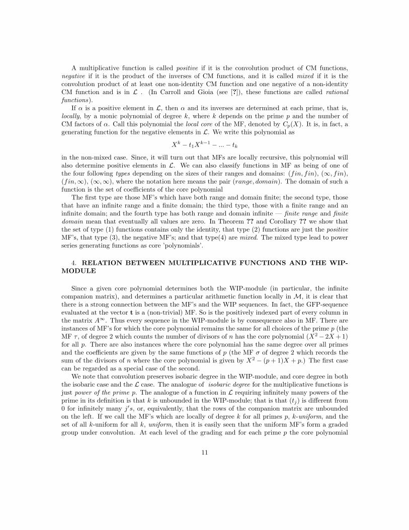
If α is a positive element in L, then α and its inverses are determined at each prime, that is,locally, by a monic polynomial of degree k, where k depends on the prime p and the number ofCM factors of α. Call this polynomial the local core of the MF, denoted by Cp(X). It is, in fact, agenerating function for the negative elements in L. We write this polynomial as

Xk − t1Xk−1 − ...− tk

in the non-mixed case. Since, it will turn out that MFs are locally recursive, this polynomial willalso determine positive elements in L. We can also classify functions in MF as being of one ofthe four following types depending on the sizes of their ranges and domains: (fin, fin), (∞, fin),(fin,∞), (∞,∞), where the notation here means the pair (range, domain). The domain of such afunction is the set of coefficients of the core polynomial

The first type are those MF’s which have both range and domain finite; the second type, thosethat have an infinite range and a finite domain; the third type, those with a finite range and aninfinite domain; and the fourth type has both range and domain infinite — finite range and finitedomain mean that eventually all values are zero. In Theorem ?? and Corollary ?? we show thatthe set of type (1) functions contains only the identity, that type (2) functions are just the positiveMF’s, that type (3), the negative MF’s; and that type(4) are mixed. The mixed type lead to powerseries generating functions as core ’polynomials’.

4. RELATION BETWEEN MULTIPLICATIVE FUNCTIONS AND THE WIP-MODULE

Since a given core polynomial determines both the WIP-module (in particular, the infinitecompanion matrix), and determines a particular arithmetic function locally in M, it is clear thatthere is a strong connection between the MF’s and the WIP sequences. In fact, the GFP-sequenceevaluated at the vector t is a (non-trivial) MF. So is the positively indexed part of every column inthe matrix A∞. Thus every sequence in the WIP-module is by consequence also in MF. There areinstances of MF’s for which the core polynomial remains the same for all choices of the prime p (theMF τ , of degree 2 which counts the number of divisors of n has the core polynomial (X2− 2X + 1)for all p. There are also instances where the core polynomial has the same degree over all primesand the coefficients are given by the same functions of p (the MF σ of degree 2 which records thesum of the divisors of n where the core polynomial is given by X2 − (p+ 1)X + p.) The first casecan be regarded as a special case of the second.

We note that convolution preserves isobaric degree in the WIP-module, and core degree in boththe isobaric case and the L case. The analogue of isobaric degree for the multiplicative functions isjust power of the prime p. The analogue of a function in L requiring infinitely many powers of theprime in its definition is that k is unbounded in the WIP-module; that is that (tj) is different from0 for infinitely many j′s, or, equivalently, that the rows of the companion matrix are unboundedon the left. If we call the MF’s which are locally of degree k for all primes p, k-uniform, and theset of all k-uniform for all k, uniform, then it is easily seen that the uniform MF’s form a gradedgroup under convolution. At each level of the grading and for each prime p the core polynomial

11

induces a (cyclic) direct summand (the values of the MF at the powers of the prime p) and, at thesame time, on the induced GFP. That is, for each k the subgroup at that level is a direct sum ofcyclic subgroups, one such subgroup for each p. We refer to these subgroups as the local subgroupsof degree k. These subgroups all have the same generic core, i.e., the cores of the elements in thesubgroup are evaluations of the same generic polynomial.

So far we have glossed over the point that the output of the functions Fk,n depends upon thechoice of domain ring. It is clear that the output of such evaluations will always be elements inthe same ring as that of the input; for examples an input of integers yields an output of integers.Integer inputs will often be used in the examples simply because so many classical MF’s are of thatsort. In general, if the evaluation ring is R (a subring of the complex numbers), we denote thesubgroup in M that they generate, MR.

With these remarks, we state the main theorem, the Correspondence Theorem.

Theorem 1 Given a prime p, let χ ∈ M with local core C(X), k finite or infinite, and let Fk(t)be the sequence of GFP’s induced by this core, then Fk,n(t) = χ(pn).

Proof As pointed out above, for each integer k, every polynomial in the WIP-module determinedby k (i.e., whose companion matrix is ∞ × k) is a member of a k-linear recursive sequence; inparticular, the GFP-sequence is one such sequence. Thus, Fk,n =

∑kj=0 tjFk,k−j , Fk,0 = 1, where

tj , j = 1, ..., k is the set of parameters that determine the recursion. Thus , every linear recursionof degree k is determined by choosing a set of values for tj (see [?]). (k can be finite or infinite).It is clear such a choice of parameters determines a multiplicative arithmetic function locally—therecursive relation determines the convolution product.

The converse is also true; that is, each multiplicative function χ has a locally faithful represen-tation as an evaluation of F (t1, ..., tj , ...) in the GFP-sequence. For, given a prime p and the set ofvalues χ(pn) = an, we can determined the tj and Fk,j(t1, ..., tj , ...) inductively in such a way thatFk,j(t1, ..., tj) = χ(pj), j 6 k. Let χ(pj) = aj , j = 1, 2, ..., and let Fk,0 = a0 = 1. Let t1 = a1 = F1,1.Suppose that tj for j < n+ 1 has been defined and that aj = Fk,j < n+ 1. We define tn+1 by

tn+1 = an −n∑j=1

tjaj−1.

That is,

tn+1 = χ(pn)−n−1∑j=1

tjχ(pj−1)

(cf. Proposition ??)

= Fn+1,n+1 −n∑j=1

tjFn,n−j+1.

The theorem now follows by the recursive property of the GFP sequence and induction. We shall use the notation χ↔ F to mean that χ is the MF that corresponds to F in the sense

of Theorem ??. The last equation in the proof reflects the fact that Fk+1,k+1−Fk,k+1 = tk+1. Thisis an example of the conservation principle referred to in Section 1. applied to the GFP sequence.The very fact that the construction in the proof of Theorem ?? is possible guarantees, by the way,that every multiplicative function is recursive.

12

A useful way of formulating the content of Theorem 1, is that each core polynomial of degreek induces k columns of linear recursions which can be taken as the k generators of a Z -moduleof linear recursions each of which is locally a multiplicative arithmetic function induced by thecoefficients of the core polynomial. The generators are produced by taking the successive powers ofthe companion matrix associated with the core polynomial (producing the k×∞ infinite companionmatrix).

An immediate consequence of Lemma ?? and the Correspondence Theorem is the following factabout multiplicative functions:

Theorem 2 A multiplicative function is periodic if and only if every root of the core polynomialis a complex root of unity. On the other hand, every multiplicative function is periodic modulo theprime (p) for every rational prime p. The p-period of the multiplicative function satisfies cp[t] 6 pk

On the other hand, it is a simple consequence of the pigeonhole principle that every multiplicativefunction is locally periodic at each prime p.

Proposition 2 [?]If the core polynomial is of degree k, then

cp[t] = cp[t1, ..., tk] 6 pk − 1.

5. EXAMPLES

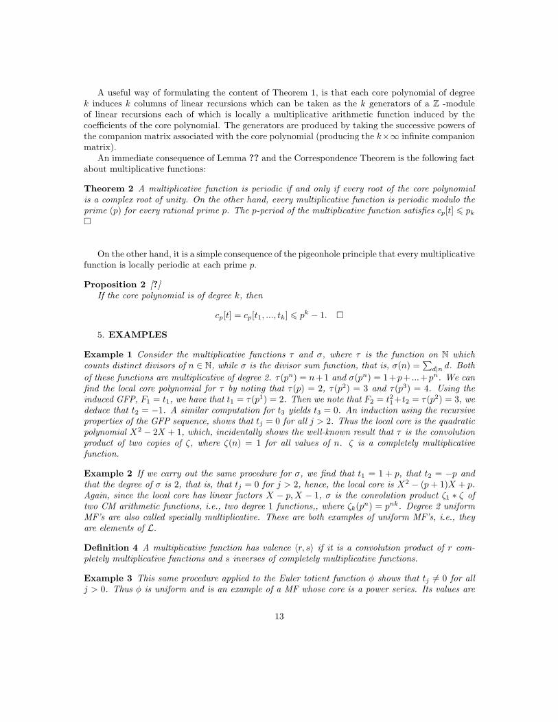
Example 1 Consider the multiplicative functions τ and σ, where τ is the function on N whichcounts distinct divisors of n ∈ N, while σ is the divisor sum function, that is, σ(n) =

∑d|n d. Both

of these functions are multiplicative of degree 2. τ(pn) = n+ 1 and σ(pn) = 1 +p+ ...+pn. We canfind the local core polynomial for τ by noting that τ(p) = 2, τ(p2) = 3 and τ(p3) = 4. Using theinduced GFP, F1 = t1, we have that t1 = τ(p1) = 2. Then we note that F2 = t21 +t2 = τ(p2) = 3, wededuce that t2 = −1. A similar computation for t3 yields t3 = 0. An induction using the recursiveproperties of the GFP sequence, shows that tj = 0 for all j > 2. Thus the local core is the quadraticpolynomial X2 − 2X + 1, which, incidentally shows the well-known result that τ is the convolutionproduct of two copies of ζ, where ζ(n) = 1 for all values of n. ζ is a completely multiplicativefunction.

Example 2 If we carry out the same procedure for σ, we find that t1 = 1 + p, that t2 = −p andthat the degree of σ is 2, that is, that tj = 0 for j > 2, hence, the local core is X2 − (p+ 1)X + p.Again, since the local core has linear factors X − p,X − 1, σ is the convolution product ζ1 ∗ ζ oftwo CM arithmetic functions, i.e., two degree 1 functions,, where ζk(pn) = pnk. Degree 2 uniformMF’s are also called specially multiplicative. These are both examples of uniform MF’s, i.e., theyare elements of L.

Definition 4 A multiplicative function has valence 〈r, s〉 if it is a convolution product of r com-pletely multiplicative functions and s inverses of completely multiplicative functions.

Example 3 This same procedure applied to the Euler totient function φ shows that tj 6= 0 for allj > 0. Thus φ is uniform and is an example of a MF whose core is a power series. Its values are

13

given by Fk,n(t1, ..., tk, ...), tj = p− 1 for all j > 0 and all k > 0 and all primes p. It is well knownthat φ = ζ1 ∗ µ, where µ is the convolution inverse of ζ, i.e. φ = ζ1 ∗ ζ−1, which is called in [?] afunction of valence 〈1, 1〉 (see Definition ??) and type (∞,∞).

This example leads to an interesting theorem:

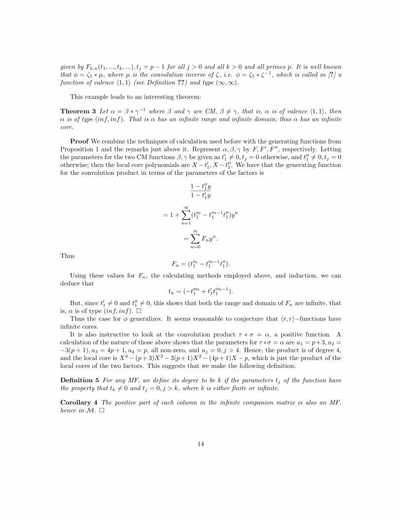
Theorem 3 Let α = β ∗ γ−1 where β and γ are CM, β 6= γ, that is, α is of valence 〈1, 1〉, thenα is of type (inf, inf). That is α has an infinite range and infinite domain; thus α has an infinitecore.

Proof We combine the techniques of calculation used before with the generating functions fromProposition 1 and the remarks just above it. Represent α, β, γ by F, F ′, F ′′, respectively. Lettingthe parameters for the two CM functions β, γ be given as t′1 6= 0, tj = 0 otherwise, and t′′1 6= 0, tj = 0otherwise; then the local core polynomials are X− t′1, X− t′′1 . We have that the generating functionfor the convolution product in terms of the parameters of the factors is

1− t′′1y1− t′1y

= 1 +∞∑n=1

(t′n1 − t′n−11 t′′1)yn

=∞∑n=0

Fnyn.

ThusFn = (t′n1 − t′n−1

1 t′′1).

Using these values for Fn, the calculating methods employed above, and induction, we candeduce that

tn = (−t′′n1 + t′1t′′n−11 ).

But, since t′1 6= 0 and t′′1 6= 0, this shows that both the range and domain of Fn are infinite, thatis, α is of type (inf, inf).

Thus the case for φ generalizes. It seems reasonable to conjecture that 〈r, r〉−functions haveinfinite cores.

It is also instructive to look at the convolution product τ ∗ σ = α, a positive function. Acalculation of the nature of those above shows that the parameters for τ ∗σ = α are u1 = p+3, u2 =−3(p + 1), u3 = 4p + 1, u4 = p, all non-zero, and uj = 0, j > 4. Hence, the product is of degree 4,and the local core is X4− (p+ 3)X3− 3(p+ 1)X2− (4p+ 1)X − p, which is just the product of thelocal cores of the two factors. This suggests that we make the following definition:

Definition 5 For any MF, we define its degree to be k if the parameters tj of the function havethe property that tk 6= 0 and tj = 0, j > k, where k is either finite or infinite.

Corollary 4 The positive part of each column in the infinite companion matrix is also an MF,hence in M.

14

Since the GFPs with non-negative indexes are now understood as corresponding to the elementsof MF, and since the properties of the GFPs naturally extend the range of the MFs to negativepowers of the prime p, it seems reasonable to extend the group L to a larger group L∗ to reflectthis fact. Moreover, the negative part of each column in the infinite companion matrix is also inMF. So we have the following situation. The core polynomial determines, a principal MF, the onedetermined in Theorem ?? by the GFP, and at the same time (a module of) induced MF’s, thosedetermined by all of the sequences in the WIP-module.

The fact that each column in the infinite companion matrix is a k-linear recursion is reflectedin the fact that the induced MF’s are determined locally by the first k powers of the prime, whilethe rest of the sequence is determined by linear recursion, the recursion constants being given bythe vector t.

In [?] it was shown that, in the case that the local core is irreducible, there is a strong relationbetween the WIP-Module and the number fields associated with the field extension determinedby the local core. This fact gives a three-way relation among the three structures: WIP-Module,multiplicative arithmetic functions and number fields. In particular, it associates with every suchnumber field, a special set of multiplicative functions.

Another question arises from the fact that the UFD A∗ has a rich ideal structure [?, ?]. Is therea representation of these ideals in terms of symmetric polynomials?

6. SPECIALLY MULTIPLICATIVE ARITHMETIC FUNCTIONS

Remark 2 The main point in this section is that there is nothing special about specially multi-plicative functions. Expressions of the sort contained in the McCarthy theorem discussed below aretrue for every multiplicative function and merely represent the fact that these functions are degreek recursive. The B(p)−term in the degree 2 case (that is, −t2) can be replaced by −t2, ...,−tk inthe degree k−case. The representation of B in terms of the original function generalizes to therepresentation t2, ..., tk as a function of its associated F-polynomials as indicated in Proposition 5above.

McCarthy’s Theorem (see P.J. McCarthy [?]) states that a multiplicative function χ is speciallymultiplicative, that is, is of degree 2, if and only if for each prime p,

χ(pn+1) = χ(p)χ(pn)− χ(pn−1)B(p),

where B(p) = χ(p)2 − χ(p2), and B(p) ∈ CM . Furthermore, degree 2 multiplicative arithmeticfunctions are characterized by the property that they admit a Busche-Ramanujan identity (see [?]).

Using Theorem 1 to translate these results into isobaric form, we get as a characterization ofdegree 2 MF’s the following:

F2,n+1(t1, t2) = t1F2,n(t1, t2) + t2F2,n−1(t1, t2),

or more succinctly,Fn+1 = t1Fn + t2Fn−1.

In particular, Bχ = B(p) = χ(p)2 − χ(p2) translates into −t2 = F 21 − F2. Indeed, using the

main theorem of this paper, this is just the redundant statement that degree 2 cores induce linearrecursions of degree 2.

15

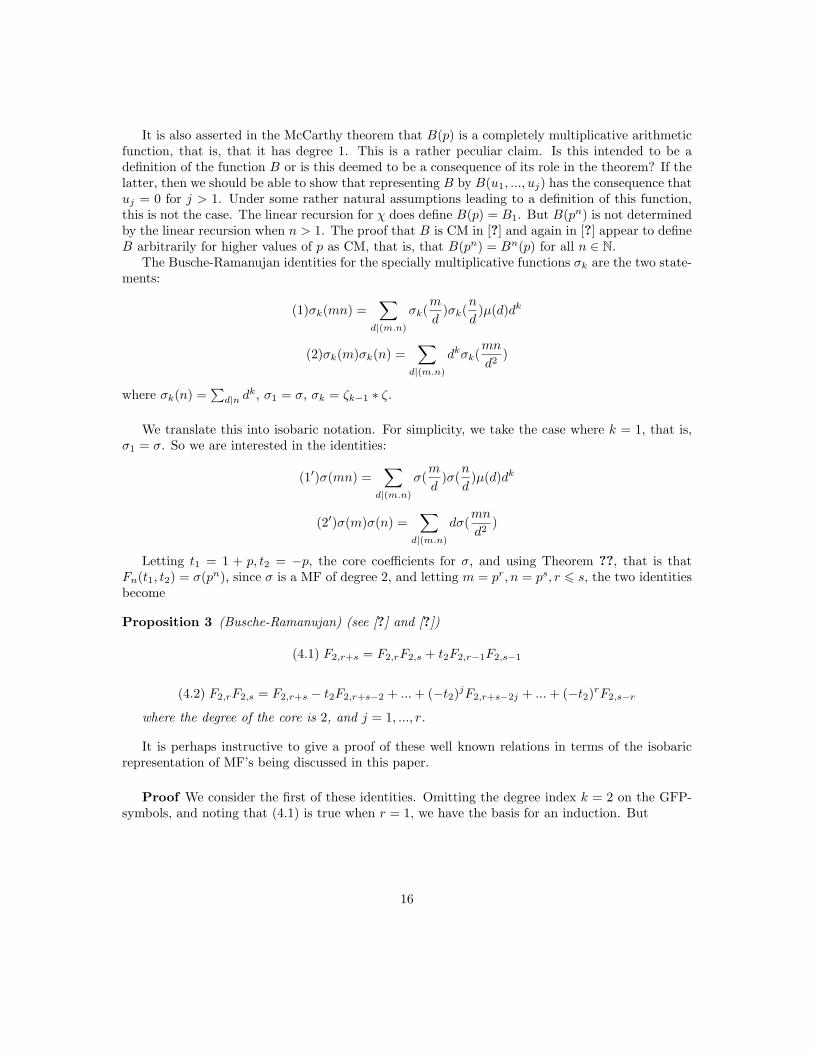
It is also asserted in the McCarthy theorem that B(p) is a completely multiplicative arithmeticfunction, that is, that it has degree 1. This is a rather peculiar claim. Is this intended to be adefinition of the function B or is this deemed to be a consequence of its role in the theorem? If thelatter, then we should be able to show that representing B by B(u1, ..., uj) has the consequence thatuj = 0 for j > 1. Under some rather natural assumptions leading to a definition of this function,this is not the case. The linear recursion for χ does define B(p) = B1. But B(pn) is not determinedby the linear recursion when n > 1. The proof that B is CM in [?] and again in [?] appear to defineB arbitrarily for higher values of p as CM, that is, that B(pn) = Bn(p) for all n ∈ N.

The Busche-Ramanujan identities for the specially multiplicative functions σk are the two state-ments:

(1)σk(mn) =∑

d|(m.n)

σk(m

d)σk(

n

d)µ(d)dk

(2)σk(m)σk(n) =∑

d|(m.n)

dkσk(mn

d2)

where σk(n) =∑d|n d

k, σ1 = σ, σk = ζk−1 ∗ ζ.

We translate this into isobaric notation. For simplicity, we take the case where k = 1, that is,σ1 = σ. So we are interested in the identities:

(1′)σ(mn) =∑

d|(m.n)

σ(m

d)σ(

n

d)µ(d)dk

(2′)σ(m)σ(n) =∑

d|(m.n)

dσ(mn

d2)

Letting t1 = 1 + p, t2 = −p, the core coefficients for σ, and using Theorem ??, that is thatFn(t1, t2) = σ(pn), since σ is a MF of degree 2, and letting m = pr, n = ps, r 6 s, the two identitiesbecome

Proposition 3 (Busche-Ramanujan) (see [?] and [?])

(4.1) F2,r+s = F2,rF2,s + t2F2,r−1F2,s−1

(4.2) F2,rF2,s = F2,r+s − t2F2,r+s−2 + ...+ (−t2)jF2,r+s−2j + ...+ (−t2)rF2,s−r

where the degree of the core is 2, and j = 1, ..., r.

It is perhaps instructive to give a proof of these well known relations in terms of the isobaricrepresentation of MF’s being discussed in this paper.

Proof We consider the first of these identities. Omitting the degree index k = 2 on the GFP-symbols, and noting that (4.1) is true when r = 1, we have the basis for an induction. But

16

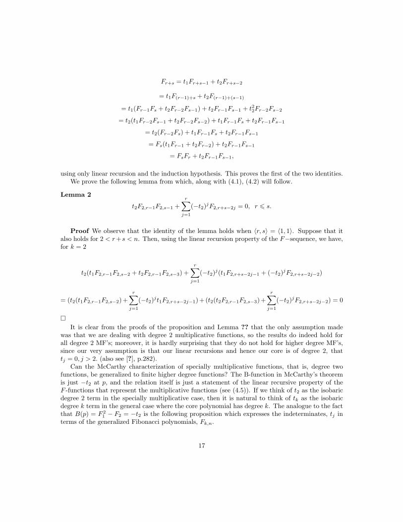
Fr+s = t1Fr+s−1 + t2Fr+s−2

= t1F(r−1)+s + t2F(r−1)+(s−1)

= t1(Fr−1Fs + t2Fr−2Fs−1) + t2Fr−1Fs−1 + t22Fr−2Fs−2

= t2(t1Fr−2Fs−1 + t2Fr−2Fs−2) + t1Fr−1Fs + t2Fr−1Fs−1

= t2(Fr−2Fs) + t1Fr−1Fs + t2Fr−1Fs−1

= Fs(t1Fr−1 + t2Fr−2) + t2Fr−1Fs−1

= FsFr + t2Fr−1Fs−1,

using only linear recursion and the induction hypothesis. This proves the first of the two identities.We prove the following lemma from which, along with (4.1), (4.2) will follow.

Lemma 2

t2F2,r−1F2,s−1 +r∑j=1

(−t2)jF2,r+s−2j = 0, r 6 s.

Proof We observe that the identity of the lemma holds when 〈r, s〉 = 〈1, 1〉. Suppose that italso holds for 2 < r+s < n. Then, using the linear recursion property of the F−sequence, we have,for k = 2

t2(t1F2,r−1F2,s−2 + t2F2,r−1F2,s−3) +r∑j=1

(−t2)j(t1F2,r+s−2j−1 + (−t2)jF2,r+s−2j−2)

= (t2(t1F2,r−1F2,s−2) +r∑j=1

(−t2)jt1F2,r+s−2j−1) + (t2(t2F2,r−1F2,s−3) +r∑j=1

(−t2)jF2,r+s−2j−2) = 0

It is clear from the proofs of the proposition and Lemma ?? that the only assumption made

was that we are dealing with degree 2 multiplicative functions, so the results do indeed hold forall degree 2 MF’s; moreover, it is hardly surprising that they do not hold for higher degree MF’s,since our very assumption is that our linear recursions and hence our core is of degree 2, thattj = 0, j > 2. (also see [?], p.282).

Can the McCarthy characterization of specially multiplicative functions, that is, degree twofunctions, be generalized to finite higher degree functions? The B-function in McCarthy’s theoremis just −t2 at p, and the relation itself is just a statement of the linear recursive property of theF -functions that represent the multiplicative functions (see (4.5)). If we think of t2 as the isobaricdegree 2 term in the specially multiplicative case, then it is natural to think of tk as the isobaricdegree k term in the general case where the core polynomial has degree k. The analogue to the factthat B(p) = F 2

1 − F2 = −t2 is the following proposition which expresses the indeterminates, tj interms of the generalized Fibonacci polynomials, Fk,n.

17

Proposition 4 Consider the GFP Fn(t1, ..., tk) and make the substitution tj = (−1)j+1Fj,thentn = Fn(F1, ..., (−1)j+1Fj , ..., (−1)n+1Fn), j = 1, 2, ..., n.

Prooftn = (−1)n+1S(1,1n−1) where S(1,1n−1) is the Schur-hook polynomial determined by the Young

diagram with arm length 1 and leg length n − 1, i.e. a vertical strip of length n, written on theisobaric basis. Using the Jacobiy-Trudi formula applied to the GFPs, we have

S(1,1n−1) = det

F1 F2 ... Fn1 F1 ... Fn−1

... ... ... ...0 0 ... F1

= (−1)n−1tn.

Here are some examples:

1. t1 = F1,

2. −t2 = F 21 − F2,

3. t3 = F 31 − 2F1F2 + F3,

Proposition ?? expresses the Busche-Ramanujan identities in terms of the GFP-representation,which in turn suggests a way of generalizing such identities to MF’s of higher degree. Thus, oneway to think of the Busche-Ramanujan identities is as an expression of Fr+s in terms of Fr and Fstogether with a remainder term. In Theorem ?? near the end of the next section, Section 7, wehave just such a generalization, which has the pleasant property of involving Schur-hook functionsas coefficients.

7. STRUCTURE OF THE CONVOLUTION GROUP M OF MULTIPLICATIVEFUNCTIONS REVISITED

The group L generated by the completely multiplicative functions, sometimes called the groupof rational functions (e.g., see [?] or [?]) contains elements of four kinds: the identity, positiveelements (the semi-group generated by CM functions), negative functions (the inverses of the postivefunctions), and mixed elements (those which are convolution products of both positive and negativeelements) as discussed in Section 2. Each element has a degree which is either infinite or a non-negative integer. The identity has degree 0, a positive element has positive degree, the degree ofits core polynomial, or, equivalently, the number of CM functions of which it is a product. (In [?]it is shown that the CM functions freely generate a free abelian group). Both negative functionsand mixed functions have infinite degrees. Negative functions have power series cores, and a mixedfunction has a rational function for a core whose numerator is the core of the positive part andwhose denominator is the core of the negative part.

In Section 2, the classification of elements of types (fin, fin), (∞, fin), (fin,∞), (∞,∞) inthe groupM was introduced, where finite range or domain means that the sequence is eventuallyconstantly zero. Infinite means that the sequence has infinitely many non-zero values.

Clearly, the types are mutually exclusive; moreover, each type is non-empty. For example, theidentity function is type 1. Type 2 consists of the positive functions, and type 3, the negativefunctions. Completely multiplicative functions, e.g., ζ, or any specially multiplicative function is

18

of type 2, e.g., σ, while µ, a negative function, is of type 3, and, as we shall see, the Euler totientfunction, φ, is of type 4 .

We now regard the tj as a set of values so that F is a particular numerical sequence F (t),and, hence, a particular MF.

Proposition 5 Let α ∈ MF and let α↔ F and let tj be the set of parameters for F . Let sjbe the set of parameters for F−1 which represents α−1, then for all j

Fj = −sj , F−1j = −tj ,

Proof 0 = F1 ∗ F−11 = F1 + F−1

1 = t1 + s1, so t1 = −s1; therefore,

F1 = −s1, and F−11 = −t1.

So assume inductively that Fj = −sj , j = 2, ..., n− 1 and that F−1j = −tj , j = 2, ..., n− 1, then we

have that

Fn =n−1∑j=1

tjFn−j + tn

= −n−1∑j=1

tjsn−j + tn.

Similarly,

F−1n = −

n−1∑j=1

tjsn−j + sn,

therefore,Fn − F−1

n = tn − sn.

Also,

Fn ∗ F−1n = Fn +

n−1∑j=1

Fn−jF−1j + F−1

n

= Fn −n−1∑j=1

sn−jt−1j + F−1

n = 0.

Thus

Fn + F−1n = −

n−1∑j=1

tjsn−j = Fn − tn = F−1n − sn.

So2Fn = Fn − sn

impliesFn = −sn,

and similarly,F−1n = −tn.

19

Corollary 5 Let F = F ′ ∗ F ′′ with t′j , t′′j being the parameters of F ′, F ′′ and s′j , s

′′j the values of

F ′, F ′′, then(1)

−sn = −s′n +n−1∑j=1

s′n−js′′j − s′′n

(2)

−tn = −t′n +n−1∑j=1

t′n−jt′′j − t′′n

equivalently

(1’)

Fn = −s′n +n−1∑j=1

s′n−js′′j − s′′n;

and

(2’)

tn = t′n −n−1∑j=1

t′n−jt′′j + t′′n.

ProofExpand the convolution product Fn =

∑nj=0 F

′n−jF

′′j and apply the theorem to the factors.

Theorem 6(3.1) core(α1 ∗ α2) = core(α1)core(α2)

(3.2) deg(α1 ∗ α2) = deg(α1) + deg(α2)

Proof.From Corollary ?? we have

−tn = −t′n +n−1∑j=1

t′n−jt′′j − t′′n.

But the −tj are just the coefficients of the core polynomial of the convolution product α1 ∗ α2;while −t′j and −t′′j are, respectively, the coefficients of the core polynomials of α1 and of α2.Thus, Corollary ?? is, at the same time, the formula for the coefficients of the core polynomial ofthe convolution product and of the coefficients of the product of the core polynomials core(α1) andcore(α2). This proves (3.1). (3.2) follows directly from (3.1) .

Definition 6 A convolution product of r + s factors is said to be in normal form if there are rdegree 1 (i.e., completely multiplicative) factors and s inverses of degree 1 factors, and if no twofactors in the product are mutually inverse to one another. By commutativity we can always writethe positive (degree 1) factors first.

20

Theorem 7 Let α ∈ MF

(1) α is type 1 = (fin, fin) if and only if it is the identity.

(2) if α is positive it is type 2, (∞, fin); if α is negative, it is type 3 .

Proof(1) Suppose that α and α−1 have a finite range, i.e., both α(pn) and α−1(pn) have value zero

for all values of n > s > 0. Let F represent α and F ′ represent α−1. Suppose that tm and Fn arethe largest non-zero values of F and −F ′, i.e. suppose that tm 6= 0 and Fn 6= 0, but that tj = 0and ti = 0 whenever j > m > 0 and i > n > 0, then consider the following equation resulting fromthe linear recursion property of the GFPs.

Fm+n = t1Fm+n−1...+ tmFn + tm+1Fn−1 + ...+ tm+nF0

Observe that the only term that survives on the right-hand side of the equation is the termtmFn, while the left-hand side is 0. So either tm or Fm is not equal 0, a contradiction to whichthe convolution identity function is exempt. Thus we have four mutually exclusive types, type 1containing only the identity. (2) claims that functions with valence < r, 0 > have infinite rangesand finite domains; while functions with valence < 0, s > have finite ranges and infinite domains.But these two propositions follow from the fact that we have defined functions to be positive if theyare a product of CM functions, and negative if they are the inverses of a product of CM functions,from Theorem ??, and from the fact that the core polynomials determine the number of parametersof a function.

Remark 3 We shall show that φ is of type 4. To show that φ is of type 4, we must show that bothφ and φ−1 have infinite non-zero range. But, for any prime p and all n, φ(pn) = pn − pn−1 6= 0.φ−1 is also infinite: its parameters are tj = −(p − 1) for all n . So let us suppose that tj = p − 1for 0 < j < n. Then, by the recursive property of GFP-sequence and induction, we have thatFn = t1Fn−1 + t2Fn−2 + ...+ tn−1F1 + tn, that is,

tn (1)= Fn − (t1Fn−1 + t2Fn−2 + ...+ tn−1F1 + tn) (2)= pn − pn−1 − (p− 1)(pn−1 − pn−2 + pn−2 + ...+ (p− 1)) (3)= pn − pn−1 − (p− 1)(pn−1 − 1) (4)= p− 1 (5)

Thus we have shown that tj = p− 1 6= 0 for all j, and so F j = −tj 6= 0 for all j, and thus thatφ ∈ type 4.

We can also prove this by using the fact that φ = ζ1 ∗ µ. Represent ζ1 by F ′ and µ by F ′′, thenby Corollary ??, t′1 = p, t′j = 0, j > 1; s′n = −pn; s′′n = −p, when n = 1, and 0 otherwise, and t′′n = 1for all values of n. We can symbolize the product by (∞, finite) ∗ (finite,∞) .

This property of φ turns out to be true for all totient functions, i.e., functions of valence 〈1, 1〉.

21

Proposition 6 α = β ∗ γ−1 where β, γ are degree 1 functions, α is not the identity function thenα is type (∞,∞) and degree ∞.

Proof. We represent α, β, and γ by, respectively, F, F ′, and F ′′, with tj , t′j , t′′j ; sj , s′j , s

′′j as in

Corollary ??. We observe that F ′n = t′n1 , and F′′n = t′′n1 , and that neither of these values is 0. We

also have that Fn = t′n1 − t′n−11 t′′1 , since t′′j = 0, j > 1, and Fn = 0, implies t′1 = t′′1 , contradicting

the hypothesis; hence, the range of α is infinite. If we apply similar reasoning to F−1n , we find that

it also has infinite range, thus α is of type 4 and has infinite degree.

In [?], Corollary 2.4, 2005, Laohakosol and Pabhapote discussed Busche-Ramanujan identitiesand the Kesava Menon norm. We shall discuss the Kesava Menon norm in the next section. Nowwe wish to look at their theorem extending Busche-Ramanujan identities to multiplicative functionsof mixed type, which we reproduce here.

Corollary 8 Let χ ∈MF, Then the following hold.(i) χ has valence 〈1, 1〉 ⇐⇒ for each prime p and each n ∈ N, there exists a complex number

T (p) such thatχ(pn) = T (p)n−1χ(p).

(ii) χ has valence 〈2, 0〉 ⇐⇒ for each prime p and each n(> 2) ∈ N,

χ(pn+1) = χ(p)χ(pn) + χ(pn−1)[χ(p2)− χ(p)2].

(iii) χ has valence 〈1, s〉 ⇐⇒ for each prime p and each χ ∈ N, there exist complex numbersB1(p), ..., Bs(p) such that for all χ > s,

χ(pn) =s∑j=0

ρ(p)n−jHj

whereHj = (−1)j

∑16i1<i2<...ij6s

Bi1(p)...Bij (p), H0 = 1.

ρ ∈ CM .

First we note that (ii) is just McCarthy’s theorem (see [?]) discussed in section 5, where weshowed that B(p) is the parameter −t2 of the positive degree two multiplicative function in question.We look now at parts (i) and (iii) of the Laohakosol-Pabhapote corollary. We shall, as is consistentwith our practice in this paper, drop reference to the prime p since our theory is instrinsically local.So we now look at part (i).

Let χ = θ ∗ ρ−1 where θ, ρ ∈ CM . (Recall the discussion of the Euler totient function ϕ above.)Let

F (t)↔ χ, F ′(t′)↔ θ, F ′′(t′′)↔ ρ.

Thent′1 6= 0, t′j = 0, j > 1; t′′1 6= 0, t′′j = 0, j > 1

Making use of Proposition ??, we have that

s′′ = F ′′n = −t′′1 if n = 1,= 0 if n > 1,

22

From this we easily deduce that:

F1 = t′1 − t′′1 = t1,

...,

Fn = (t′)(n−1)1 (t′1 − t′′1) = t

′(n−1)1 (t′1 − t′′1) = t

′(n−1)1 t1 = t′(n−1)F1

That is,

Proposition 7 Suppose χ = θ ∗ρ−1, θ and ρ degree 1 functions, θ 6= ρ and θ 6= δ 6= ρ, and supposethat χ, θ, and ρ are represented by, respectively, F, F ′, and F ′′, with parameters tj , t′j , t

′′j ; sj , s′j , s

′′j .

Then,Fn = t

′(n−1)1 F1, ∀n ∈ N

where F′′

= F−1.

Thus, the mysterious T (p) in the original corollary is just one of the parameters determiningthe representing GFP-sequence just as in the case of McCarthy’s theorem, this time for θ, it is justt′1.

Next, we look at part (iii) of the corollary. We first consider a product of degree 3, as in Remark3, i.e., a product χ = θ ∗ ρ−2 where θ is a positive function of degree 1, and ρ is a positive functionof degree 2, and use the formalism of the previous example for representing χ, θ and ρ by GFPsequences. Thus we have

F (t1, t2, t3) = F ′(t′1) ∗ F ′′(t′′1 , t′′2).

(Here we are thinking of F′′

not as an inverse, but as a function in its own right). With the helpof Proposition ?? and Corollary ??, we easily find that

F1 = t′1 + t′′1 = t1

andF2 = F ′2 + F ′1F

′′1 + F

′′2 = t′21 + t′1t

′′1 + t′′2

= t′1(t′1 + t′′1) = t′1F1 − s′′2 .

In the same way,F3 = t′21 F1 − t′1s′′2 − s′′3 .

Induction gives us

Proposition 8 If χ has valence〈1, s〉 and χ↔ F then

Fn = (t′)n−1F1 − t′n−21 s′′2 − t′n−3

1 s′′3 .

The proposition is nothing but a thinly disguised version of the definition of convolution prod-uct together with the particular assumptions about the parameters of the factors together withProposition ??. But it says all that the Laohakosol-Pabhapote result says and at the same time ex-plicitly identifies the mysterious functions. Compare the previous remarks concerning the McCarthytheorem. The general case is now clear.

23

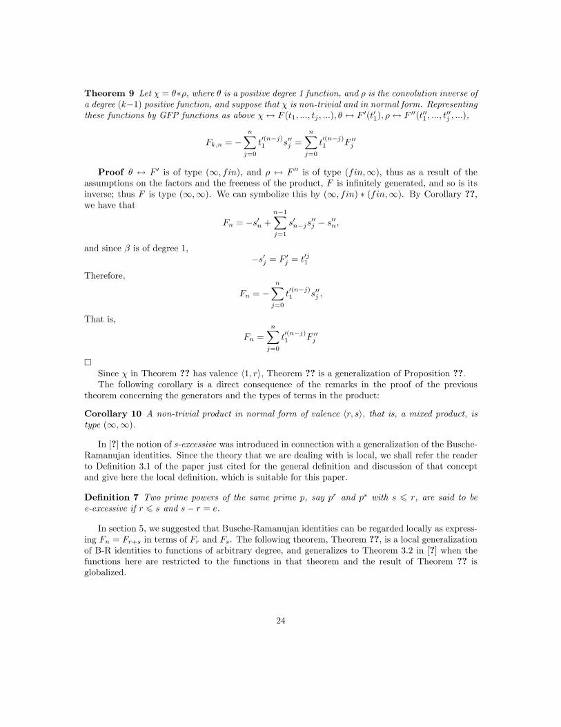
Theorem 9 Let χ = θ∗ρ, where θ is a positive degree 1 function, and ρ is the convolution inverse ofa degree (k−1) positive function, and suppose that χ is non-trivial and in normal form. Representingthese functions by GFP functions as above χ↔ F (t1, ..., tj , ...), θ ↔ F ′(t′1), ρ↔ F ′′(t′′1 , ..., t

′′j , ...),

Fk,n = −n∑j=0

t′(n−j)1 s′′j =

n∑j=0

t′(n−j)1 F ′′j

Proof θ ↔ F ′ is of type (∞, fin), and ρ ↔ F ′′ is of type (fin,∞), thus as a result of theassumptions on the factors and the freeness of the product, F is infinitely generated, and so is itsinverse; thus F is type (∞,∞). We can symbolize this by (∞, fin) ∗ (fin,∞). By Corollary ??,we have that

Fn = −s′n +n−1∑j=1

s′n−js′′j − s′′n,

and since β is of degree 1,−s′j = F ′j = t′j1

Therefore,

Fn = −n∑j=0

t′(n−j)1 s′′j ,

That is,

Fn =n∑j=0

t′(n−j)1 F ′′j

Since χ in Theorem ?? has valence 〈1, r〉, Theorem ?? is a generalization of Proposition ??.The following corollary is a direct consequence of the remarks in the proof of the previous

theorem concerning the generators and the types of terms in the product:

Corollary 10 A non-trivial product in normal form of valence 〈r, s〉, that is, a mixed product, istype (∞,∞).

In [?] the notion of s-excessive was introduced in connection with a generalization of the Busche-Ramanujan identities. Since the theory that we are dealing with is local, we shall refer the readerto Definition 3.1 of the paper just cited for the general definition and discussion of that conceptand give here the local definition, which is suitable for this paper.

Definition 7 Two prime powers of the same prime p, say pr and ps with s 6 r, are said to bee-excessive if r 6 s and s− r = e.

In section 5, we suggested that Busche-Ramanujan identities can be regarded locally as express-ing Fn = Fr+s in terms of Fr and Fs. The following theorem, Theorem ??, is a local generalizationof B-R identities to functions of arbitrary degree, and generalizes to Theorem 3.2 in [?] when thefunctions here are restricted to the functions in that theorem and the result of Theorem ?? isglobalized.

24

Theorem 11 Let α be a multiplicative arithmetic function of degree k, and let r and s be twointegers with r 6 s, and abbreviating Fk,n as Fn, then

Fn = Fr+s =e+1∑j=0

(−1)jS(r,1j)Fs−j .

where S(r,1j) is an isobaric reflect of the Schur-hook function whose Young diagram has an arm oflength r and a leg length of j.

Observe that these Schur-hook functions for a given r consist exactly of the elements of the r-th row,in order from right to left, of the companion matrix, and that S(r,10) = Fr; so that this formulasatisfies our interpretation of a generalization of the Busche-Ramanujan identity, and includesTheorem 3.2 in [?]. Also observe that such a row is a vector representing the r-th power of a rootof the core polynomial (see section 2).

Proof (of Theorem ??)First note that the companion matrix is stable in the sense that adding a k+1-st column on the

left of an ∞× k−companion matrix changes nothing in the original matrix. Thus we might as wellassume that we have infinitely many parameters for F . For a finite k we need only let tj = 0 froma certain point onward. We shall also need to recall the fact that the columns of the companionmatrix are linear recursions with respect to the parameters tj . When r = 0 the theorem is just astatement of the fact that F is a linear recursion with parameters tj . We proceed by induction onr with e = r − s.

Fn = Fr+s = t1F(r−1)+s + t2F(r−2)+s + ...+ tkF(r−k)+s

= t1

e+2∑j=0

S(r−1,1j)Fs−j + t2

e+3∑j=0

S(r−2,1j)Fs−j + ...+e+k+1∑j=0

S(r−k,1j)Fs−j

= (e+2∑j=0

t1S(r−1,1j) +e+3∑j=0

t2S(r−2,1j) + ...+e+k+1∑j=0

tkS(r−k,1j))Fs−j

=e+1∑j=0

S(r,1j)Fs−j

Corollary 2.6 in [?] simply states that for a positive function of degree r, tj = 0, j > r, tr 6= 0.And Corollary 2.7 in [?] is a statement of the basic fact that the representing GFP-sequence is ak-order linear recursion whenever α is a multiplicative function of degree k, (see [?] or, indeed, [?],[?], and [?]).

To conclude this section, we point out that in the formalism of this paper, using symmetricfunction theory, some classical theorems in multiplicative number theory reduce to rather prosaicstatements, if not trivialities. An example of this is the binomial identity, (see [?], [?],[?]). Wewould like to use this instance to show how this is the case.

The binomial identity may be stated as follows:

Proposition 9 Suppose that α = γ1 ∗ γ2 where γ1 and γ2 are completely multiplicative functions,then α satisfies the binomial identity

α(pn) =dn

2 e∑j=0

(−1)j(n− jj

)α(p)n−2j(γ1(p)γ2(p))j ,

25

which in turn is just a special case of the general formula for Weighted Isobaric Polynomials, (see[?]). If we use our GFP representation, then this result is just a case of the general formula forGFP’s as in section 1 of this paper; namely,

Fk,n =∑α`n

(|α|

α1, ..., αk

)tα11 ...tαk

k .

Here is the formulation in our terms:

Proposition 10 Let α be a positive MF of degree 2 represented by F , and let F ′ and F ′′ representthe convolution factors, then

F2,n = Fn =dn

2 e∑j=0

(−1)j(n− jj

)Fn−2j

1 (−t′1t′′1)j .

Thus, we have

Fn =dn

2 e∑j=0

(−1)j(n− jj

)Fn−2j

1 (−t2)j .

As an example, let n = 5, and note that the partitions of 5 with k = 2 are just (15), (13, 2), (1, 22).Then, we have,

F2,5 =3∑j=0

(−1)j(

5− jj

)F 5−2j

1 (−t2)j = t51 + 4t31t2 + 3t1t22.

8. KESAVA MENON NORM

Since our aim is to show the utility of expressing multiplicative function theory in terms ofisobaric polynomials, we include a discussion of the Kesava Menon norm. The Kesava Menon normN is defined on multiplicative functions and is given by

N (α)(n) =∑d|n2

α(n2)λ(d)α(d)

where λ is the Liouville function. N is a multiplicative function. The Liouville function is definedby λ(m) = (−1)Ω(m), where Ω(m) is the number of prime factors of m counting the multiplicity ofa prime in m; in particular, λ(pn) = 1 if n is even and −1 if n is odd. If α has degree 1 or 2, thendegN (α) = 1, 2, respectively. What does the norm look like in isobaric notation?

Let Fn(t)↔ α, α ∈MF for suitable choice of the vector t, and let N (Fn) = N (α)(pn). Then

N (Fn) =2n∑j=0

(−1)jF2n−jFj

or, equivalently

N (Fn) = 2n−1∑j=0

(−1)jF2n−jFj + (−1)nF 2n

By Corollary ??, (1’) and (2’), this can be written in the following way.

26

Proposition 11

N (Fn) = −2s2n + 2n−1∑j=1

(−1)js2n−jsj + (−1)ns2n

N (Fn) = 2t2n + 2n−1∑j=1

(−1)jt2n−jtj + (−1)nt2n.

It is well known that this norm is multiplicative (see [?], p.50), that is, that: If α and β ∈ MF,then

N (α ∗ β) = N (α) ∗ N (β).

We give a proof here using the concepts of this paper .First, we observe that

N (F ′0 ∗ F ′′0 ) = F ′0F′′0 = F ′′0 = N (F0) = 1 = N0.

.We prove the following lemma:

Lemma 3 If F1 = F ′1 ∗ F ′′1 , then

N (F1) = N (F ′1 ∗ F ′′1 ) = N (F ′1) ∗ N (F ′′1 )

Proof Let χ = χ′ ∗ χ′′ where χ, χ′, χ′′ are multiplicative functions, and let χ ↔ F, χ′ ↔ F ′, andχ′′ ↔ F ′′. Using the definition we have

N1(F ) = 2F2 − F 21 = 2(t21 + t2)− t21 = t21 + 2t2

Then using Corollary ??, we have

(t′1 + t′′1)2 + 2(t′2 − t′1t′′1 + t′′2) = t′12 + 2t′1t

′′1 + t′′1

2 + 2t′2 − 2t′1t′′1 + 2t′′2

= (t′12 + 2t′2) + (t′′1

2 + 2t′′2)

which isN1(F ′) +N1(F ′′),

andN1(F ′) +N1(F ′′) = N ′1 ∗ N ′′1

Theorem 12 Let F = F ′ ∗ F ′′, then

N (Fn) = N (F ′n) ∗ N (F ′′n );

that is, if Nn = N (Fn), thenNn = N ′n ∗ N ′′n

27

Proof It is well known that the KM-norm is a multiplicative function, and hence by the correspon-dence theorem is linearly recursive. Denoting the indeterminates of the MFs N , N ′ and N ′′ by nr,n′r and n′′r , and using Corollary ??, we have

nr = n′r −r−1∑j=1

n′jn′′r−j + n′′r ,

where 1 6 j 6 rThen, using the recursion property of the norm function, we have

Nr =r∑j=1

njNr−j =r∑j=1

(n′j −r−j∑s=1

n′r−j−sn′′s + n′′j )Nr−j .

where 1 6 s 6 r.We let nu = 0 when u < 0 and nu = 1 when u = 0 .By the inductive hypothesis:

Nr−j = N ′r−j ∗ N ′′r−j ,

we have

Nr =r∑j=1

(n′j −r−j∑s=1

n′r−j−sn′′s + n′′j )

r∑j=1

N ′r−j ∗ N ′′e−j

and so

=r∑j=1

[(n′j −j−1∑s=1

n′j−sn′′s + n′′j )(

r−j∑i=0

N ′r−j−iN ′′i)],

where 0 6 s 6 r. Thus, we have

Nr =r∑j=1

[(n′j + n′′j )r∑j=1

N ′r−j−iN ′′i − (j−1∑s=1

n′j−sn′′s

r−j∑i=0

N ′r−j−iN ′′i.)],

which we can write as

Nr =r∑j=1

(n′j

r−j∑i=0

N ′r−j−iN ′′i) +r∑j=1

(n′′j

r−j∑i=0

N ′r−j−iN ′′i)− (r∑j=1

(j−1∑s=1

n′j−sn′′s

r−j∑i=0

N ′r−j−iN ′′i.)).

We can now shift the order of summation in the first and second summands on the right handside, and using the fact that N ′0 = 1 and N ′′0 = 1,

28

Nr =r∑i=0

(n′jr−i∑j=1

N ′r−j−iN ′′i)

+r∑i=0

(n′′jr−i∑j=1

N ′′r−j−iN ′i) +r−2∑j=1

n′j(N′′r−j −

r−j∑i=1

n′′jN′′r−j−i)

+(r−2∑j=1

n′′j (N ′r−j −r−j∑i=1

n′jN′r−j−i).

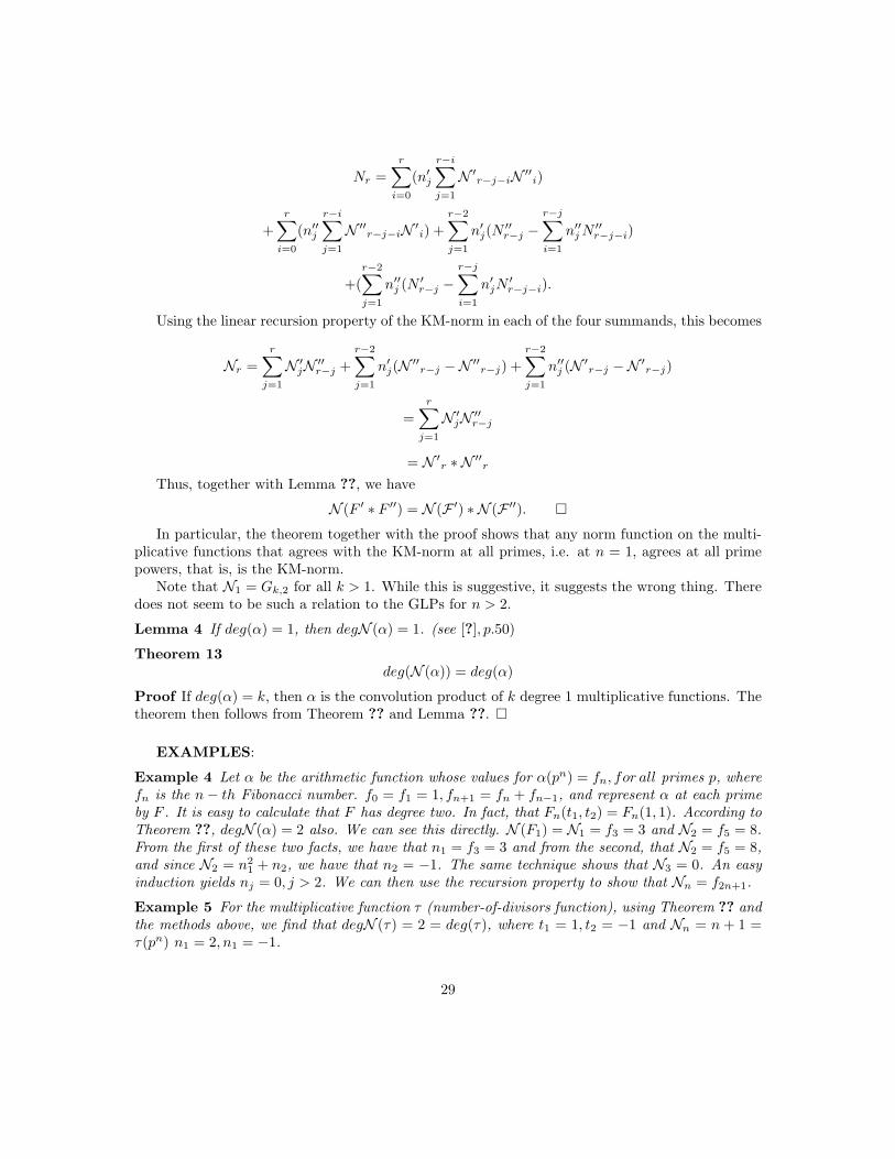
Using the linear recursion property of the KM-norm in each of the four summands, this becomes

Nr =r∑j=1

N ′jN ′′r−j +r−2∑j=1

n′j(N ′′r−j −N ′′r−j) +r−2∑j=1

n′′j (N ′r−j −N ′r−j)

=r∑j=1

N ′jN ′′r−j

= N ′r ∗ N ′′rThus, together with Lemma ??, we have

N (F ′ ∗ F ′′) = N (F ′) ∗ N (F ′′).

In particular, the theorem together with the proof shows that any norm function on the multi-plicative functions that agrees with the KM-norm at all primes, i.e. at n = 1, agrees at all primepowers, that is, is the KM-norm.

Note that N1 = Gk,2 for all k > 1. While this is suggestive, it suggests the wrong thing. Theredoes not seem to be such a relation to the GLPs for n > 2.

Lemma 4 If deg(α) = 1, then degN (α) = 1. (see [?], p.50)

Theorem 13deg(N (α)) = deg(α)

Proof If deg(α) = k, then α is the convolution product of k degree 1 multiplicative functions. Thetheorem then follows from Theorem ?? and Lemma ??.

EXAMPLES:

Example 4 Let α be the arithmetic function whose values for α(pn) = fn, for all primes p, wherefn is the n− th Fibonacci number. f0 = f1 = 1, fn+1 = fn + fn−1, and represent α at each primeby F . It is easy to calculate that F has degree two. In fact, that Fn(t1, t2) = Fn(1, 1). According toTheorem ??, degN (α) = 2 also. We can see this directly. N (F1) = N1 = f3 = 3 and N2 = f5 = 8.From the first of these two facts, we have that n1 = f3 = 3 and from the second, that N2 = f5 = 8,and since N2 = n2

1 + n2, we have that n2 = −1. The same technique shows that N3 = 0. An easyinduction yields nj = 0, j > 2. We can then use the recursion property to show that Nn = f2n+1.

Example 5 For the multiplicative function τ (number-of-divisors function), using Theorem ?? andthe methods above, we find that degN (τ) = 2 = deg(τ), where t1 = 1, t2 = −1 and Nn = n + 1 =τ(pn) n1 = 2, n1 = −1.

29

References

[1] George E. Andrews, Euler’s Parititio Numerorum, Bu.Am.Math.Soc., 44(2007), no.4, 561-573.

[2] T.B. Carroll, A characterization of completely multiplicative arithmetic functions, Amer. Math.Monthly 81 (1974), no 9, 993-995.

[3] T.B. Carroll and A.A. Gioia, On a subgroup of the group of multiplicative arithmetic functions,J.Austral.Math.Soc. Ser. A 20 (1975), no.3, 348-358.

[4] E.D. Cashwell and C.J. Everett, The ring of number theoretic functions, Pacific J. Math. 9(1959), no.4, 975-985.

[5] Y.C. Chen and James D. Louck, The Combinatorial Power of the Companion Matrix, LinearAlgebra and its Applications, 232, (1996) 261–268.

[6] Graham Everest, Alf van der Poorten, Igor Schparlinski, Thomas Ward, Recurrence SequencesAMS Mathematical Monographs and Surveys, 104, (2003).

[7] Umberto Cerruti and Vaccarino, Francesco, Vector linear recurrence sequences in commutativerings, Applications of Fibonacci numbers, Vol.6 (Pullman,WA,1994),63-72, Kluwer Acad.Publ.,Dordrecht, 1996.

[8] P.Haukkanen, Binomial formulas for specially multiplicative functions, Math.Student64(1995), no.1-4 155-161.

[9] P.Haukkanen, Some characterizations of totients, Int.J.M.Math. Math. Sci. 19 (1996), no.3,209-217.

[10] P.Haukkanen, On the real powers of completely multiplicative functions, Nieuw Arch. Wiskd.(4) 15 (1997), no. 1-2, 73-77.

[11] P.Haukkanen, Rational arithmetic functions of order (2,1) with respect to regular convolu-tions,Port.Math. 56 (1999), no. 3, 329-343.

[12] P.Haukkanen, Some characterizations of specially multiplicative functions, Int.J.Math.Math.Sci (2003), no. 37, 2335-2344.

[13] P.Haukkanen,On convolution of linearly recurring sequences and finite fields , J. Algebra 149(1992), 179-182.

[14] P.Haukkanen, On convolution of linearly recurring sequences and finite fields, II,J. Algebra164 (1994), 542-544.

[15] Qing-hu Hou and Yang-ping Mu, Recurrent Sequences and Schur functions, Advances in Ap-plied Mathematics, 31 (2003) 150-162.

[16] V.Laohakosol, N.Pabhapote, N. Wechwiriyakul, Logarithmic operators and characterizationsof completely multiplicative functions Southeast Asian Bull.Math. 25 (2001) no.2, 273-281.

[17] Laohakosol, N.Pabhapote,Properties of rational arithmetic functions, Journal of Mathematicsand Mathematical Sciences 2005:24 (2005) 3997-4017.

30

[18] V.Laohakosol, N.Pabhapote, N. Wechwiriyakul, Characterizing completely multiplicative func-tions by generalized Mobius functions Int.J.Math. Math. Sci 24 (2005), no,11, 3997-4017.

[19] A. Lascoux, Suites recurrentes lineaires, Adv. in Appl. Math. 7, (1986) 228-235.

[20] A. Lascoux, Symmetric Functions, Nankai University, December 2001, http//www.combinatorics.net/teach.

[21] I.G. Macdonald, Symmetric Functions and Hall Polynomials, Clarendon Press, Oxford, 1995.

[22] T. MacHenry, A Subgroup of the Group of Units in the Ring of Arithmetic Functions, RockyMountain Journal of Mathematics ,29, (1999), 1055-1065.

[23] T. MacHenry, Generalized Fibonacci and Lucas Polynomials and Multiplicative ArithmeticFunctions, Fibonacci Quarterly, 38, (2000), 17-24.

[24] Trueman MacHenry and Geanina Tudose, Reflections on Isobaric Polynomials and ArithmeticFunctions, Rocky Mountain Journal of Mathematics, Vol.35, No.3, 2005, pp.901-928.

[25] T. MacHenry and G. Tudose, Differential Operators and Weighted Isobaric Polynomials, RockyMountain Journal of Mathematics, Vol 36 N6 (2006) p1957-1976 .

[26] T. MacHenry and Kieh Wong, Degree k Linear Recursions Mod(p) and Number Fields, RockyMountain Journal of Mathematics, to appear.

[27] P.J. McCarthy, Introduction to Arithmetical Functions, Unversitext, Springer, New York. 1986.

[28] K.G. Ramanathan: Multiplicative Arithmetic Functions J. Ind. Math. Soc. 7 (1943), 157-82

[29] D. Rearick. Operators on algebras of arithmetic functions, Duke Math.J. 35 (1968), no. 4,761-766.

[30] D. Rearick, The trigonometry of numbers, Duke Math.J. 35 (1968), no. 4, 767-776.

[31] D.Redman and R. Sivaramakrishnan, Some properties of specially multiplicative functions,, J.Number Theory 13 (1981), no.2, 210-227.

[32] J. Rutkowski, On recurrence characterization of rational arithmetic functions, Funct. Approx.Comment. Math. 9 (1980), 45-47.

[33] H.N. Shapiro, On the Convolution Ring of Arithmetic Functions, Communications of Pure andApplied Mathematics, vol. xxv, (1972), 287-336.

[34] R. Sivaramakrishnan, On a class of multiplicative arithmetic functions. J. reine angew. math.280 (1976), 157-82.

[35] R. Sivaramakrishnan, Classical theory of Arithmetic functions, Monographs and Textbooks inPure and Applied Mathematics, vol. 126, Marcel Dekker, New York, 1989.

[36] R.Vaidyanathaswamy, The theory of multiplicative arithmetic functions,Trans. Amer. Math.Soc. 33 (1931),no.2, 579-662.

31

Key Words: multiplicative arithmetic functions, symmetric polynomials, isobaric basis, linearrecursions generalized Fibonacci sequences. O5EO5,11B37,11B39,11N99

Trueman MacHenryYork University, Toronto, Canadamachenry@mathstat.yorku.ca

Kieh WongCentennial College, Toronto, Canadakkwong@centennialcollege.ca

April 14, 2009

32