a credit risk model for albania · bank of greece economic research department – special studies...
TRANSCRIPT

BANK OF GREECE
EUROSYSTEM
Special Conference PaperSpecial Conference Paper
FEBRUARY 2011
A credit risk model for Albania
Kliti Ceca Hilda Shijaku
Discussion: Faidon Kalfaoglou
7

BANK OF GREECE Economic Research Department – Special Studies Division 21, Ε. Venizelos Avenue GR-102 50 Athens Τel: +30210-320 3610 Fax: +30210-320 2432 www.bankofgreece.gr Printed in Athens, Greece at the Bank of Greece Printing Works. All rights reserved. Reproduction for educational and non-commercial purposes is permitted provided that the source is acknowledged. ISSN 1792-6564

Editorial
On 19-21 November 2009, the Bank of Greece co-organised with the Bank of
Albania the 3rd Annual South Eastern European Economic Research Workshop held at its
premises in Athens. The 1st and 2nd workshops were organised by the Bank of Albania
and took place in Tirana in 2007 and 2008, respectively. The main objectives of these
workshops are to further economic research in South Eastern Europe (SEE) and extend
knowledge of the country-specific features of the economies in the region. Moreover, the
workshops enhance regional cooperation through the sharing of scientific knowledge and
the provision of opportunities for cooperative research.
The 2009 workshop placed a special emphasis on three important topics for central
banking in transition and small open SEE economies: financial and economic stability;
banking and finance; internal and external vulnerabilities. Researchers from central banks
participated, presenting and discussing their work.
The 4th Annual SEE Economic Research Workshop was organised by the Bank of
Albania and took place on 18-19 November 2010 in Tirana. An emphasis was placed
upon the lessons drawn from the global crisis and its effects on the SEE macroeconomic
and financial sectors; adjustment of internal and external imbalances; and the new
anchors for economic policy.
The papers presented, with their discussions, at the 2009 SEE Workshop are being
made available to a wider audience through the Special Conference Paper Series of the
Bank of Greece.
Here we present the paper by Hilda Shijaku (Bank of Albania) and Kliti Ceca (Bank
of Albania) with its discussion by Faidon Kalfaoglou (Bank of Greece).
February, 2011
Altin Tanku (Bank of Albania) Sophia Lazaretou (Bank of Greece) (on behalf of the organisers)


A CREDIT RISK MODEL FOR ALBANIA
Hilda Shijaku Bank of Albania
Kliti Ceca
Bank of Albania
ABSTRACT Our methodology takes into account existing methods of stress testing for credit risk for the system as a whole, and adapts them to the Albanian financial intermediation features and data. The model starts by testing the presence of a system of equations (stationary VAR) capturing the joint behaviour of financial and real variables. The equation is modelled to contain some dynamics allowing for the persistence of shocks over more than one period given the backward looking nature of the chosen proxy for the default rate. In the second step, by using Monte Carlo simulations we propose generating the distribution of losses of the default rates. We relax the assumption of zero error terms in the reduced form estimates in step one and simulate univariate/multivariate normally distributed vectors of error terms via Monte Carlo methods, where the information on the variance/covariance matrix is obtained from the reduced form equations in step one. Next, we introduce a shock to the nonfinancial variable (growth rate, interest rates, exchange rates etc.) and similarly compute a range of values for the default rate in the stressed scenario. JEL classification: C51, E58. Keywords: stress testing, credit risk Acknowledgments: We would like to thank the participants of the 3rd SEE Workshop for a useful exchange discussion. Special thanks are due to our discussant Faidon Kalfaoglou for his valuable comments and suggestions. The views expressed in this paper are those of the authors and do not necessarily reflect those of the Bank of Albania and the Bank of Greece. We alone are responsible for the remaining errors and omissions. Correspondence: Hilda Shijaku Financial Stability Department Kliti Ceca Department of Research Bank of Albania, “Sheshi Skënderbej”, Nr.1, Tirana, Albania. Email: [email protected] and [email protected]


1. Introduction
Stress tests are a very important tool for assessing the ability of economic agents to
offset the impact of large shocks on their wealth. In the aftermath of the world’s biggest
financial crisis since the Great Depression, there is an ever increasing interest in stress
testing financial intermediaries to assess their capital needs in the event of large but
plausible shocks. The extensive debate about stress tests has covered issues of
aggregation/disaggregation of stress tests, top-down versus bottom-up approaches and
modelling strategies. The various approaches are considered as complementary rather
than substitutes as they serve different needs. However, central banks have an important
role in all cases by either setting basic standards and coordinating stress tests at the micro
level, or tailoring them to assess the financial stability implications of macroeconomic
developments and systematic risk.
In this paper, we devise a macro stress test for Albania assessing the impact of the
direct and indirect credit risk channels using aggregate data. This stress test could be used
as a satellite to the existing macroeconomic model in the Bank of Albania (BoA) that
may help in examining the macroeconomic implications of the scenarios derived by the
latter. The paper builds on an existing methodology of the top-down approach at the BoA
(Financial Sector Assessment Program, FSAP) and proposes a different modelling
strategy to identify the channels. The main contribution is the parameterisation of the
impact of macroeconomic factors on credit quality for the Albanian banking system. We
also propose a method for the assessment of a range of measures of portfolio
deterioration under various scenarios integrating a measure of uncertainty in the above
assessment.
The paper proceeds as follows. In Section 2, we conduct a review of the existing
literature on macro stress tests in order to identify a suitable strategy for our investigation.
In Section 3, we outline the existing FSAP methodology, identify areas for improvement
and present our approach and research hypotheses. In Section 3, we explain the empirical
estimation and discuss the results. In Section 4, we conduct an exercise using the data for
September 2008. Finally, Section 5 presents the main conclusion of the analysis and the
7

limitations of the research followed, and mentions possible areas for further
improvement.
2. A review of the literature
This section looks at the modelling strategies used for stress testing credit risk. By
critically reviewing the various stages of the analysis, we identify the advantages and the
disadvantages of each of the choices made, in order to select a strategy for our own model
and acknowledge the possible limitations.
Stress testing is an increasingly popular method of analysing the resilience of
financial systems to adverse events. According to Cihak (2007), stress testing as a process
includes: (i) the identification of specific vulnerabilities or areas of concern; (ii) the
construction of a scenario; (iii) the mapping of the output of the chosen scenario into a
form that is usable for an analysis of the balance sheet and the income statement of the
financial institutions; (iv) the performance of the numerical analysis; (v) the consideration
of any second round effects; and (vi) the summary and the interpretation of the results. In
particular, stress tests for credit risk focus on the risk that a borrower may be unable to
repay its debt under specific conditions. Quantifying this risk has advanced markedly
since the late 1990s with the development and dissemination of models for measuring
credit risk on a portfolio basis.
Sorge and Virolainen (2006) make a distinction between two classes of stress
testing models. The first refers to the ‘piecewise approach’, in which a direct relationship
between the macroeconomic variables and the indicators of financial soundness is
estimated (balance sheet models). The estimated parameters of these models can be used
later to simulate the impact of severe scenarios on the financial system. Balance sheet
models can be either structural or reduced-form ones. The other class of models concerns
the ‘integrated approach’, in which multiple risk factors (credit, market risk etc.) are
combined to estimate the probability distribution of aggregate losses that could arise in a
stress scenario. Several studies have modelled default probabilities as non-linear
functions of macro variables (Wilson 1997) or have incorporated them into a value-at-
risk (VaR) measure (Sorge and Virolainen 2006).
8

In a review of the stress testing techniques for credit risk, Foglia (2009) and Cihak
(2007) summarize the stages in a macro stress test as shown in Figure 1.
Figure 1. Summary of the stages in a macro stress test
Source: The figure is adapted from Foglia (2009).
In the first stage, a stress event arising from exogenous factors is identified. The
stress event can be thought as a shock which affects the domestic economy and which is
very large, but still possible. Then, these shocks are used to produce a scenario for the
macroeconomic environment. A common way to execute this stage is to use a
macroeconometric model. Given that macroeconometric models do not typically include
financial sector variables, the stress testing framework is extended to include separate
‘satellite’ models which transmit the effects of macroeconomic variables to ‘key’
financial intermediation responses (such as credit growth) and, in a third stage, link the
latter together with macroeconomic variables to financial sector measures of asset quality
9

and potential credit losses. The losses are then used to derive the buffers of profit and
capital under various scenarios.
The effects of the stress scenario on macroeconomic conditions are typically
measured using (i) a structural econometric model; (ii) vector autoregressive methods;
and/or (iii) pure statistical approaches (Foglia 2009).
Existing structural macroeconomic models (such as those used by the central bank
for forecasts and policy analysis) are used to project the levels of key macroeconomic
indicators under various scenarios including a set of initial exogenous inputs over a given
scenario horizon. Typically all FSAPs use macroeconomic models used for monetary
policy purposes and in some cases are extended to incorporate international effects
(Foglia 2009). The main advantage in using structural macroeconomic models lies in the
fact that they impose consistency across the predicted values in the stress scenario.
Moreover, they may allow for endogenous policy reactions to the initial shock. A major
problem of these modelling strategies is that they are primarily devised for ‘normal
business’ times and the linearity embedded in them may fail to adequately represent the
nonlinear behaviour characteristic in times of stress. Further, it is difficult to determine
the likelihood of a specific scenario to implement in stress testing.
A second approach used in various central bank studies makes use of Vector
Autoregressions (VARs) or Vector Error Correction models (VECMs) to jointly combine
the effects of exogenous shocks into various macroeconomic variables which are then
used in the scenario chosen (Foglia 2009). These models are often used as an alternative
to macroeconomic models. Besides, being substitutes for them, they are relatively
flexible and produce a set of mutually consistent shocks, although they do not include the
economic structure that is incorporated in the macroeconomic modelling approach.
A third approach is used by the Oesterreichische Nationalbank (OeNB) in its
Systemic Risk Monitor (SRM), in which a purely statistical approach is used to design a
scenario. Macroeconomic and financial variables are modelled through a multivariate t-
copula. This approach has the advantage of identifying the marginal distributions which
can be different from the multivariate distribution that characterizes the joint behaviour of
the variables. In addition, the relationship between the macroeconomic variables and the
10

financial variables displays tail dependence (i.e., ‘correlation’ increases when the system
is under stress). For policy analysis purposes, however, being a purely statistical
approach, it does not identify the key transmission channels that link the shock with its
effect on the degree of credit risk.
The second stage of stress testing regards the modelling of auxiliary models that
link credit risk to the macroeconomic variables derived in stage one. These models are
estimated either for the whole system or for different levels of disaggregation such as by
industry, type of borrower (sector), bank or individual borrower. These regression models
include loan performance measures such as non-performing loans (NPL) or loan loss
provisions (LLP) as dependent variables; explanatory variables typically include a set of
macroeconomic indicators, sometimes bank/industry specific variables such as measures
of indebtedness or market-based indicators of credit risk depending on the level of
aggregation. Variables such as economic growth, unemployment, interest rates, equity
prices and corporate bond spreads contribute to explaining default risk.
Two approaches are common (Cihak 2007). One is based on data on loan
performance, such as the NPLs, the LLPs or the historical default rates; and the other is
based on micro-level data related to the default risk of the household and/or the corporate
sector. We concentrate on the former as a full discussion of all approaches is beyond the
scope of this section. In models based on loan performance, the key dependent variables
are the NPL ratio, the LLP ratio and the historical default frequencies.
Blaschke et al (2001) model unexpected credit losses arising from external shocks
by empirically estimating the determinants of observed default frequencies as captured by
NPL ratios, which can be interpreted as a default frequency ratio. They propose
regressing NPL-to-total assets ratio on a set of macroeconomic variables, including the
nominal interest rate, inflation, GDP growth and the percentage change in terms of trade.
In addition, they propose estimating this equation by using disaggregated NPL data
across homogenous groups of borrowers. If we assume linearity in the risk exposures, the
volatility of the ratio of the NPLs to total assets can be expressed as a function of the
variances of the regressors and the correlations between them. However, they recommend
the use of the Monte Carlo simulation techniques when this assumption is relaxed.
11

More recently, Castren et al (2009) study the effects of macroeconomic shocks on
VaR for different banks through two steps. First, they estimate a GVAR (Global Vector
Autoregression) model to obtain impulse responses for real Gross Domestic Product
(GDP), real stock prices, inflation, short-term and long-term interest rates and the euro-
dollar exchange rate. In the second step, the results of these macroeconomic shocks are
regressed on the sector specific probability of default (PD) values.
Van den End et al (2006) develop reduced-form balance sheet models to estimate
the impact of the macro variables on the LLPs using data for the 5 largest Dutch banks. In
modelling credit risk, they use two basic equations. First, they estimate the relationship
between borrower defaults and real GDP growth, long-term interest rates, short-term
interest rates and the term spread. In a second step, they develop a fixed effect regression
model explaining the LLPs using the default rate together with some macro variables. By
using different constant terms, the structural differences in the level of provisions for
each bank are taken into account. In the equations, non-linear functions of the default rate
and the ratio of LLPs to total credit – the logit – are used to extend the domain of the
dependent variable to negative values and take into account possible non-linear
relationships between the macro variables and the LLPs.
For the simulations, van den End et al (2006) use the version developed by Sorge
and Virolainen (2006), who simulate default rates over time by generating
macroeconomic shocks to the system. The evolution of the related macroeconomic
shocks is given by a set of univariate autoregressive equations of order 2, i.e. AR(2), or
alternatively, by a VAR model. The latter model takes into account the correlations
between the macro variables. Van den End et al (2006) use the vector of innovations and
a variance-covariance matrix of errors in the equations governing the macroeconomic
variables, and in the default rate and LLP/credit equations. By using a Cholesky
decomposition of the variance-covariance matrix, they are able to obtain correlated
innovations in the macroeconomic factors, default rate and LLP/CRED, and obtain future
paths of the macroeconomic variables, the default rate and LLP/CRED by simulation
with a Monte Carlo method. With these outcomes and the information on outstanding
exposures of the banking sector, the distributions of credit losses are determined. The
12

simulated distributions of losses are skewed to the right, due to the correlation structure
of the innovations.
Wong et al (2006) study the effects of macro variables on total credit risk and
mortgage credit risk in Hong Kong. Their model involves the construction of two
macroeconomic credit risk models, each consisting of a multiple regression model and a
set of autoregressive models which include feedback effects from the default rate on bank
loans to different macroeconomic values estimated by the method of the seemingly
unrelated regression. The stress testing framework uses the models developed by Wilson
(1997a, 1997b), Boss (2002) and Virolainen (2004), and allows for a more realistic
dynamic process in which the macroeconomic variables are mutually dependent. Most
importantly, it explicitly captures the feedback effects of bank performance on the
economy by letting the macroeconomic variables depend on past values of the financial
variables. The set of equations define a system of equations governing the joint evolution
of macroeconomic performance, the associated default rates and their error terms. By
taking non-zero error terms in the default rate equation and allowing for randomness in
the behaviour of the macroeconomic variables with the various stochastic components
being correlated, Wong et al take into account the probabilistic elements and use Monte-
Carlo simulation to obtain frequency distributions for the default ratios in various
scenarios. The default rate is hypothesised to depend on the real GDP growth of Hong
Kong, the real GDP growth of mainland China, real interest rates and real property prices
in Hong Kong. Non-linearities are taken into account by using a logit transformation of
the NPL ratio and first differences are used to avoid spurious regression in the presence
of non-stationarity in the variables.
Though there is an extensive use of loan performance data to measure credit quality
in the literature, several considerations are applied (Foglia 2009). Loan performance as
measured by the NPLs or the LLPs is a ‘retrospective’ indicator of asset quality because
it reflects past defaults. Provision rules in addition to varying across countries may also
pose a problem for ‘within country’ estimation as they may vary with changes in credit
risk in time, bank-specific factors or the use of income-smoothing policies.
13

Another frequent problem in interpreting macroeconomic models of credit risk
concerns the use of linear statistical models. In the majority of cases this is solved by
using non-linear specifications, such as the logit and the probit transformation to model
the default rate. These transformations extend the domain of the dependent variable to
negative values and take into account possible non-linear relationships between
macroeconomic variables and the default rate that are likely in stress situations. Several
other studies on stress testing models take non-linearities into account by including
squares and cubes of the macroeconomic variables (Drehmann et al 2005).
3. The methodology of stress testing in Albania
The methodology of stress testing for credit risk in the BoA is based on directly
stressing the growth in non-performing loans of the banking system and measures the
effect on the capital adequacy of the banking system. It also stresses GDP growth and
estimates its effect on the change in the NPLs of the banking system. The relation
between real GDP growth and the growth of the NPLs is assumed to be linear as shown
in equation (1)
11 /52/ −− ∆−=∆ tttt GDPGDPNPLRNPLR (1)
which implies that a shock to the nominal growth rate at a given time causes, other
things being equal, a corresponding growth of 5 times the shock in the NPL ratio
(NPLR). Under the assumption of zero growth in total loans, the relative change in NPLR
equals the relative change in NPLs.
In a second step, by assuming a zero value for e, and by shocking the GDP growth
rate of the given year, a point estimate of the growth of the NPLs is obtained. These
predicted values are (point) estimates of the expected values of the NPLs conditional on
the occurrence of the scenario.
Another scenario includes the effect on the NPLR of a currency depreciation
capturing the credit risk arising from foreign currency lending and the effects of indirect
credit risk from an increase in credit interest rates. For the former, assuming the increase
in total debt after a given currency depreciation by FXr∆ , denoted as FXD r∆⋅ , is
14

incurred all within a year and not amortized throughout the lifetime of the debt,
borrowers will face a yearly income loss proportional to the debt in foreign currency to
income ratio D/I.
Hence, the relative income change will be: FXIDI rr ∆=∆ (2)
Following (1) and assuming GDPI rr ∆=∆
we get equation (3), i.e.
FXIDBIBNPLR rr
br ∆−=∆=∆ * (3)
where B=-5 from equation (1) and the leverage D/I is assumed 2 for all currencies.
For the indirect credit risk arising from an increase in interest rates and the total
increase in debt is faced by the borrowers, the same assumption holds, i.e. all income loss
through the increase in debt is incurred within a year. By calculating the debt increase for
different remaining maturity re-pricing buckets, the corresponding NPLR equals:
DIDBIBNPLR rr
br ∆−=∆=∆ * (4)
A number of weaknesses can be identified in the above approach. First, the values
of the parameters linking GDP growth to the change in non-performing loans seem
unrealistic if we compare the fitted values with the observed values of the change in non-
performing loan growth. Hence, the conclusion drawn by stress testing is erratic and
biased downward (see Figure 2).
Second, the effect of a shock to GDP on the NPLs may not peak in the same period
and will last over some quarters, because of the interactions between industries and
various groups of agents. The present model does not include information about this.
15

Figure 2. Observed and estimated NPL growth
estimated and real NPL growth
-100%
-80%
-60%
-40%
-20%
0%
20%
40%
60%
80%
100%
120%
2000 2001 2002 2003 2004 2005 2006 2007
RealEstimated
Note: The estimated NPL is according to equation (1).
Third, the present model only provides a point estimate of the probable losses and
does not allow us to obtain the range of losses the shock may bring at a desired level of
significance. Thus, even if the predicted value of the soundness indicator is not
significantly affected by the realization of the adverse scenario, it is hard to conclude that
the risk is low because a large deviation from the average may occur with a ‘tangible’
probability. Fourth, once a scenario is chosen, how likely it is to occur is no longer an
issue in stress testing (Wong et al 2006). Finally, only one economic indicator is
modelled, yet the shock may be directly generated through a range of indicators that
influence the level of the NPLs and interact with economic growth. By inserting
dynamics in the model, we would be able to estimate which effect is bigger and the
period in which we expect it to appear.
In the next section, we construct our model by addressing the above mentioned
issues.
16

4. Methodology
Our methodology is based on Wong et al (2006). We first construct a model of
either a system of equations or single equations linking our variables of interest. In other
words, we model non-performing loans as a function of some macroeconomic variables.
Second, a Monte Carlo simulation is used to generate the distribution of losses of the
default rates under the unstressed and stressed scenarios.
The equations are modelled to contain some dynamics allowing for the persistence
of shocks over more than one period given the backward-looking nature of the chosen
proxy for the default rate and the effect’s persistence caused by the interrelations between
different industries and sectors. Empirically, the equations are estimated by means of a
stationary VAR, where exogeneity restrictions are imposed on the foreign variables only.
Otherwise, domestic macroeconomic variables are allowed to be affected by past values
of the default rate. Specifically, we test the following hypotheses:
a. The default rate both is affected by and affects the economic growth. In the
first step, we allow the effect to run from the default rate to economic growth
as there might be incentives for commercial banks to restrict credit growth
which by construction affects the default rate and negatively impacts
economically new investment and thus the growth rate.
b. The default rate is affected by changes in foreign interest rates (Euribor or
Libor rates). In this way, we model indirect foreign interest rate risk which
alters payments, and the cash flow of households and firms on loans extended
in foreign currency and linked to these interest rates.
c. The default rate is affected and affects the domestic interest rate. As in point
b, we model the indirect domestic interest rate risk.
d. The default rate is affected by the exchange rates of the Euro and USD vis-à-
vis the Albanian Lek (ALL). These variables capture deteriorations in the
credit portfolio as a result of unhedged borrowing in foreign currency.
e. The default rate is negatively affected by inflation.
17
We relax the assumption of zero error terms in the reduced form estimates and
simulate univariate/multivariate normally distributed vectors of error terms via Monte
Carlo methods, where the information on the variance-covariance matrix is obtained from
the reduced form equations. Based on the parameters estimated in the VARs and the most
updated information on the nonfinancial variables (growth rate, interest rates, exchange
rates etc), we compute a range of values for the default rate and obtain confidence levels
for the unstressed scenario. Next, we introduce a shock to one of the nonfinancial
variables (growth rate, interest rates, exchange rates etc) and similarly compute a range of
values for the default rate in the stressed scenario. Although we do not compute the
related VaR statistics as in Wong et al (2006), they can easily be derived from the model.
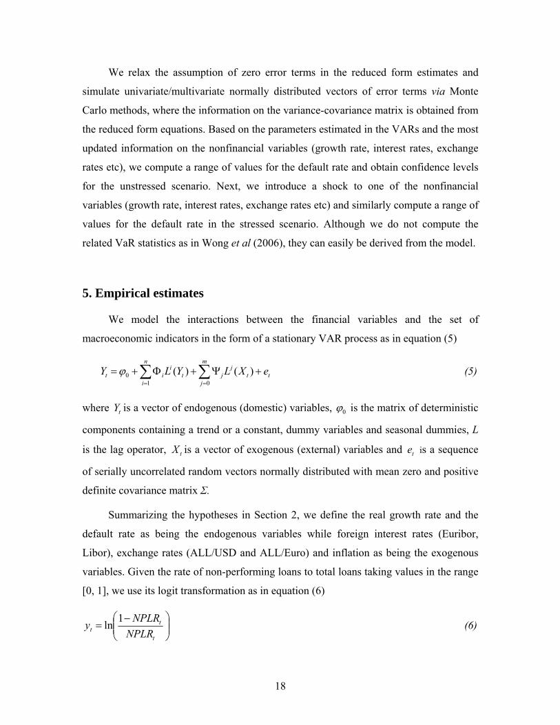
5. Empirical estimates
We model the interactions between the financial variables and the set of
macroeconomic indicators in the form of a stationary VAR process as in equation (5)
t
m
jt
jj
n
it
iit eXLYLY +Ψ+Φ+= ∑∑
== 010 )()(ϕ (5)
where is a vector of endogenous (domestic) variables, tY 0ϕ is the matrix of deterministic
components containing a trend or a constant, dummy variables and seasonal dummies, L
is the lag operator, is a vector of exogenous (external) variables and is a sequence
of serially uncorrelated random vectors normally distributed with mean zero and positive
definite covariance matrix Σ.
tX te
Summarizing the hypotheses in Section 2, we define the real growth rate and the
default rate as being the endogenous variables while foreign interest rates (Euribor,
Libor), exchange rates (ALL/USD and ALL/Euro) and inflation as being the exogenous
variables. Given the rate of non-performing loans to total loans taking values in the range
[0, 1], we use its logit transformation as in equation (6)
⎟⎟⎠
⎞⎜⎜⎝
⎛ −=
t
tt NPLR
NPLRy 1ln (6)
18

where denotes the non-performing loans ratio in period t. tNPLR
A dummy variable is included to account for the write-off of non-performing loans
in 2001Q3. Seasonal dummies are also included to alleviate potential problems with
diagnostic tests.
Before proceeding, unit root tests are conducted to ensure that the individual series
are I(0) processes. To this end, we employ ADF tests, unit root tests with a structural
break and DF-GLS tests. Given the low power of the ADF test in small samples, the lag
length is chosen as the minimum lag length for which statistical tests do not indicate
serial correlation in the residuals of the ADF specification. Saikkonen and Lütkepohl
(2002) and Lanne et al (2002) propose unit root tests for the model including
unknown/known break points, which are based on estimating the deterministic term first
by a generalized least squares (GLS) procedure under the unit root null hypothesis and
subtracting it from the original series. Then, an ADF type test is performed on the
adjusted series which also includes terms to correct for estimation errors in the
parameters of the deterministic part. The asymptotic null distribution is nonstandard and
critical values are tabulated in Lanne et al (2002). We employ this test acknowledging
that stationarity is a statistical approximation of the long-run properties of the series; if
the time span is very short, a near unit root is most likely to appear as a non-stationary
process. Similarly, we can argue that the likelihood of observing ‘structural’ changes in
the series or large shocks increases in small samples.
From the results of the unit root tests1 we may conclude that changes in nominal
interest rates and the logarithms of ALL/USD and EUR/USD exchange rates are all I(0).
Hence, a stationary VAR can be specified with these variables while avoiding spurious
relationships and the persistence of shocks in the system. In the next section, we will
present these VARs which are satisfactory both statistically and economically.
The next step in our analysis includes the generation of 20.000 numbers from a
normal distribution with mean 0 and variance obtained in step 1 using Monte Carlo
procedures for the simulation of a normal distribution. Because a large amount of random
1 Results of the tests are available on request.
19

(or pseudorandom) numbers is thus generated, we consider procedures of reduction of the
statistical errors by selecting special algorithms.
Although the theory of Monte Carlo simulation gives many formulae for the
simulation of random numbers of different distributions, serious statistical errors may
happen during the actual simulation using some algorithms. Although theoretically these
algorithms are deterministically supposed to generate random numbers from a given
distribution, their practical application may produce ‘biased’ numbers because of the
approximation given by computers. The computers work based on a limited ‘word length’
and hence obtain limited precision for numerical values of any variable. Truncation and
round-off errors may in some cases lead to serious problems of statistical quality. In
addition, there are statistical errors which arise as an inherent feature of the simulation
algorithm due to the finite number of members in the generated ‘statistical sample’. Some
of the errors may be systematic.
In the case of the VAR estimation in which residual autocorrelation is present, the
Cholesky decomposition of the variance-covariance matrix of the residuals obtained in
step 1 can be used to transform the Monte Carlo N(0,1) generated random vector into
mutually correlated shocks for our equations. Alternatively, by obtaining the error terms
from the estimation in the macroeconomic model and those for our default rate, we can
obtain the variance-covariance matrix and perform a similar exercise.
Based on the parameter estimates obtained in the VAR model and the residuals
taken using the Monte Carlo simulation, we obtain values for dy under two scenarios:
(i) the evolution of the nonfinancial variables is consistent with ‘normal business’,
i.e. no change in them or evolution according to a pattern known ex ante.
(ii) the evolution of the nonfinancial series is shocked, according to an extreme but
possible scenario.
For both scenarios we can obtain the distribution of the NPLs (after transforming
the variable dy) for a given probability.
Acknowledging the problems of inference associated with a VAR on a short data
series, the VAR order is chosen as the smallest order which satisfies VAR specification
20

tests (all using 4 lags): namely, the residuals are serially uncorrelated (on the basis of the
LM and Portmanteau tests) and are normally distributed (on the basis on the Jarque-Bera
test on skewnesses and kurtosis of the residuals, see Doornik & Hansen 1994 and
Lütkepohl 1993) with a homoscedastic variance (on the basis of the ARCH-LM test and
multivariate ARCH-LM test). Given that the VAR models are generally suitable for
estimation over a relatively homogenous period, we also present VAR stability tests, i.e.
the CUSUM and CUSUM squared tests of VAR stability.
Using different VAR orders in an iterative process, we cannot obtain meaningful
estimates (i.e. correct sign and significant parameters) of the effects of the
abovementioned variables on non-performing loan ratios. Taking into account the effect
of multicollinearity on the significance of the parameters, we proceed by estimating the
VAR models on dy and the macroeconomic variables separately in order to investigate
whether the latter can be specified as exogenous (i.e. there is no significant effect of the
lagged dy on the current macroeconomic indicators). Finally, using a parsimonious model
which excludes insignificant variables and redundant equations, the following set of
equations is obtained (see Table 1-6).
21

Table 1. Deterioration in GDP
Variable dyt dyt-1 rgt-2 dum_Bart S1 Coefficient 1 0.255 0.009 1.148 -0.137 p-Value (0.004) (0.004) (0.000) (0.008)
Table 2. Diagnostic tests
statistic p-value df Autocorelation
NA Portmaneau test (4 lag) NA
LM-type test LM 3.1251 0.5371 4 Nonnormality Doornik & Hansen (1994) joint 0.3886 0.8234 2 skewness only 0.0095 0.9224 2 kurtosis only 0.3791 0.5381 2 Lütkepohl (1993) joint 0.3886 0.8234 2 skewness only 0.0095 0.9224 2 kurtosis only 0.3791 0.5381 2 Jarque-Bera test 0.3886 0.8234 Heteroscedasticity ARCH-LM test 4.6927 0.3203 VARCHLM test 4.6927 0.3203 4
Table 3. Foreign interest rate risk
Variable dyt dyt-1 dnreut dum_Bart S1 S2 Coefficient 1 0.337 -0.126 1.143 -0.079 0.135 p-Value (0.000) (0.071) (0.000) (0.108) (0.004)
Note: sample range: [2000 Q1, 2007 Q4], T = 32
22

Table 4. Diagnostic tests
statistic p-value df Autocorelation Portmaneau test (4 lag) NA LM-type test LM 1.8708 0.7595 4 Nonnormality Doornik & Hansen (1994) joint 0.2087 0.9009 2 skewness only 0.0001 0.9934 2 kurtosis only 0.2086 0.6478 2 Lütkepohl (1993) joint 0.2087 0.9009 2 skewness only 0.0001 0.9934 2 kurtosis only 0.2086 0.6478 2 Jarque-Bera test 0.2087 0.9009 Heteroscedasticity ARCH-LM test 4.3519 0.3605 VARCHLM test 4.3519 0.3605 4
Table 5. Euro/ALL exchange rate
Variable dyt dyt-1 dlneut-1 dum_Bart S1 S2 Coefficient 1 0.0356 -2.536 1.284 -0.092 0.104 p-Value (0.000) (0.004) (0.000) (0.054) (0.025)
As is evident from these estimates, all macroeconomic variables appear exogenous
to developments in dy, though they may be related to each other. However, this can be
taken into account by constructing a scenario outside this model which accounts for the
relationship between the macroeconomic indicators (such as a macroeconomic model or
previous historical information), and then using this scenario to investigate the effect on
dy.
23

Table 6. Diagnostic tests statistic p-value df Autocorelation Portmaneau test (4 lag) NA LM-type test LM 0.6371 0.9588 4 Nonnormality Doornik & Hansen (1994) joint 0.1942 0.9075 2 skewness only 0.1039 0.7472 2 kurtosis only 0.0904 0.7637 2 Lütkepohl (1993) joint 0.1942 0.9075 2 skewness only 0.1039 0.7472 2 kurtosis only 0.0904 0.7637 2 Jarque-Bera test 0.1942 0.9075 Heteroscedasticity ARCH-LM test 7.9663 0.0928 VARCHLM test 7.9663 0.0928 4
Using the information taken from estimations in Tables 1, 3 and 5, we next
construct a nested model by specifying dy as the only endogenous variable (see Tables 7
and 8).
Table 7
Variable dyt dyt-1 dnreut-1 dlneut-1 rgt-2 dum_Bart S1 Coefficient 1 0.1.88 -0.137 2.411 0.013 1.211 -0.127 p-Value (0.064) (0.090) (0.005) (0.005) (0.00) (0.02)
Note: Residual variance: 1.321055e-02 ; Sample range: [2001 Q2, 2007 Q4], T = 27
24

Table 8. Diagnostic tests
statistic p-value df Autocorrelation Portmaneau test (4 lag) NA LM-type test LM 1.9527 0.7445 4 Nonnormality Doornik & Hansen (1994) joint 1.0941 0.5787 2 skewness only 1.0926 0.2959 2 kurtosis only 0.0014 0.9699 2 Lütkepohl (1993) joint 1.0941 0.5787 2 skewness only 1.0926 0.2959 2 kurtosis only 0.0014 0.9699 2 Jarque-Bera test 1.0941 0.5787 Heteroscedasticity ARCH-LM test 6.6670 0.1546 VARCHLM test 6.6670 0.1546 4
Figure 3. Stability tests
25

We conclude that the model is correctly specified with respect to the diagnostic
tests and the process is stable at 5 per cent significance level. We also notice that all
variables have the correct sign and are statistically significant at 5 and 10 per cent
significance levels. Credit growth appears to be importantly affected by changes in the
exchange rate and the euro interest rate while the effect of GDP deterioration seems
trivial. A possible reason for this may be the small variation in the GDP data used in the
estimation. Given that the quarterly data entries are obtained by filtering annual data,
some of the variation may have been lost, thus resulting in the true effect of GDP on dy
captured by the parameters on other coefficients.
6. Illustration
As a final step in this analysis we proceed by extracting 20.000 numbers from the N
~ (0; 02321055.1 −e ) distribution and use the parameters in Table 7 to compute the
probability distribution of dy under the stressed and unstressed scenarios.
For illustrative purposes, we present the following analysis using the data for
September 2008 and relying on the respective assumptions. We do not make use of the
stochastic components of the macroeconomic model for this illustration and allow for a
stochastic component just in the default rate. A simulation allowing for randomness in the
macroeconomic variables and using the variance-covariance between the stochastic
components in the latter and the estimated ε from this equation is subject to further
investigation.
26

Table 9. Scenarios
Given y September 3.147244 unstressed stressed Given dy September 0.047068 Given rg June 6 Given dnreu September 0.063 Given dlneu September -0.01496 Computed dy December 0.114294 Assumptions rg September 6 2 Assumptions dlneu December 0 0.182322 Assumptions dnreu December 0 1
Change in the exchange rate 0.2
Euro/ALL September 122.05
In the unstressed scenario, we assume an annual GDP growth of 6% in September,
consistent with that of the end of the year. We assume no changes in the Euribor and no
change in the exchange rate vis-a-vis the ALL. In the stressed scenario, we assume a 20
per cent depreciation of the ALL, a 100 basis points change in the Euribor and GDP
growth of 2 per cent. The estimates show that, under these assumptions, the expected
value of the NPLR of March 2009 increases from 3.82 to 6.93 per cent. From Table 10
where we present descriptive statistics of the computed NPLR under the two scenarios,
we can obtain also interval estimates of the NPLR. As an example, the 90 per cent
interval estimates change from [3.29; 4.38] to [6.00; 7.90]. Another important finding is
also the probability of encountering ‘tail’ values of the NPLR increases as shown by the
increase in the standard deviation of the stressed scenario from 0.004 to 0.007. Figure 4
presents the graphical illustration of the probability distribution.
27

Table 10. Statistics of the NPLR for the stressed and unstressed scenarios
Nplr mars09 unstress Nplr mars09 stressed Mean 3.82% 6.93%St dev 0.004270794 0.0074851535th Q 3.16% 5.77%95th Q 4.55% 8.21%10th Q 3.29% 6.00%90th Q 4.38% 7.90%15th Q 3.39% 6.17%85th Q 4.26% 7.70%20th Q 3.46% 6.29%80th Q 4.17% 7.55%
Figure 4. Probability distribution under the stressed and the unstressed scenarios
Combined scenario
0
200
400
600
800
1000
1200
2.42
%2.
71%
3.00
%3.
29%
3.58
%3.
86%
4.15
%4.
44%
4.73
%5.
02%
5.30
%5.
59%
5.88
%6.
17%
6.46
%6.
75%
7.03
%7.
32%
7.61
%7.
90%
8.19
%8.
47%
8.76
%9.
05%
9.34
%9.
63%
9.91
%10
.20%
10.4
9%10
.78%
11.0
7%11
.35%
11.6
4%11
.93%
12.2
2%12
.51%
12.7
9%13
.08%
13.3
7%13
.66%
13.9
5%14
.23%
14.5
2%14
.81%
NPLr mars unstressed
NPLr mars stressed
7. Summary and conclusions
The paper presents several improvements in the methodology of stress testing of
indirect credit risk in Albania. We find a significant effect of the changes in the euro
exchange rates and the Euribor interest rates on the non-performing loan ratio while the
effect of GDP growth, albeit small, is found to be significant too. Most importantly, our
methodology provides a measure of uncertainty of the estimates through the computation
28

of the probability distribution of the variables of interest both under the stressed and the
unstressed scenarios.
While at this stage the model seems to be satisfactory both from a theoretical and
statistical perspective, there are various ways in which this part of research could be
extended in the future. First, given our data length and the asymptotic properties of the
VAR analysis, a re-estimation of the model is necessary once a new/revised data set
comes available. Second, a VaR statistic would be obtained using several assumptions
about the evolution of total loans. However, this is beyond the main objective of this
paper. Third, estimation at a more disaggregated level would also be of great interest, as
different portfolio performances might prevail among different groups of banks, or
separately for households, businesses, mortgages, different industries, etc. Finally, the
model can also use scenarios derived from the macroeconomic model accounting for the
impact of a shock to one macroeconomic indicator may have on other macroeconomic
indicator and evaluating the effects of macroeconomic policies on the banking system.
29

References
Blaschke, W., Jones, M., Majnoni, G. and Peria, S. (2001), ‘Stress Testing of Financial Systems: An Overview of Issues’, Methodologies, and FSAP Experiences, International Monetary Fund.
Boss, M. (2002), ‘A Macroeconomic Credit Risk Model for Stress Testing the Austrian Credit Portfolio’, Financial Stability Report 4, Oesterreichische Nationalbank.
Castrén , O., Fitzpatrick, T. and Sydow, M. (2009), ‘Assessing Portfolio Credit Risk Changes in a Sample of EU Large and Complex Banking Groups in Reaction to Macroeconomic Shocks’, ECB Working Paper Series no 1002 / February.
Cihak, M. (2007), ‘Introduction to Applied Stress Testing’, IMF Working Paper no 59, International Monetary Fund.
Drehman, M. (2005), ‘A Market Based Macro Stress Test for the Corporate Credit Exposures of UK Banks’, available at www.bis.org/bcbs/events/rtf05Drehmann.pdf.
Foglia, A. (2009), ‘Stress Testing Credit Risk: A Survey of Authorities’ Approaches’, International Journal of Central Banking, 5, 9-45.
Lanne, M., Lutkepohl, H. and Saikkonen, P. (2002), Comparison of Unit Root Tests for Time Series with Level Shifts’, Journal of Time Series Analysis, 23, 667-685.
Sorge, M. (2004), ‘Stress-testing Financial Systems: An Overview of Current Methodologies’, BIS Working Papers, no 165.
Sorge, M., and Virolainen, K. (2006), ‘A Comparative Analysis of Macro Stress-Testing with Application to Finland’, Journal of Financial Stability, 2, 113–51.
Van den End, J. W., M. Hoeberichts and M. Tabbae (2006), ‘Modelling Scenario Analysis and Macro Stress-Testing’, De Nederlandsche Bank Working Paper no 119.
Virolainen, K. (2004), ‘Macro Stress-testing with a Macroeconomic Credit Risk Model for Finland’, Bank of Finland Discussion Paper no 18.
Wilson, T. (1997), ‘Portfolio Credit Risk (II)’, Risk, 10, 56-61.
Wong, J. Choi, K. and Foi, T. (2006), ‘A Framework for Macro Stress Testing the Credit Risk of Banks in Hong Kong’, Hong Kong Monetary Authority Quarterly Bulletin, December.
30

Discussion Faidon Kalfaoglou2
Bank of Greece
A stress test is commonly described as the evaluation of the financial position of a
bank under an extreme but plausible scenario in order to facilitate decision making within
the bank. Similarly, macro stress testing refers to a range of techniques used to assess the
vulnerability of a financial system to ‘exceptional but plausible’ macroeconomic shocks.
Both approaches gained significant momentum during the current financial crisis since
the importance of complementing the micro-prudential analysis with a macro-prudential
perspective has become evident. Increasingly, macro stress testing plays an important role
in the macro-prudential analysis of public authorities. The main objective is to identify
structural vulnerability and overall risk exposures in a financial system that could lead to
systemic problems. In addition, macro stress testing forms the main part of system-wide
analysis, which measures the risk exposure of the financial system to a specific stress
scenario. However, several research papers have indicated that stress test exercises
conducted before the crisis have significant vulnerabilities related to their in
formativeness, scenario severity and model robustness (see, for example, Rodrigo and
Drehmann 2009). In the de Larosier (2009) report (p8)3 it is clearly mentioned that
‘…model-based risk assessments underestimated the exposure to common shocks and tail
risks and thereby the overall risk exposure. Stress-testing too often was based on mild or
even wrong assumptions’. These conclusions, among others, initiated an increase in
research interest in macro stress testing, and the topic is rapidly evolving. The paper by
Shijaku and Ceca is a contribution to this strand of literature, particularly the applied part
which refers to the Albanian banking sector.
The model presented in the paper was initiated during an FSAP mission from the
IMF, has gone through substantial improvement and follows the traditional approach. A
2 Economic Research Department. Email:[email protected] 3 High level group on financial supervision in EU, chaired by J. de Larosier, February 2009.
31
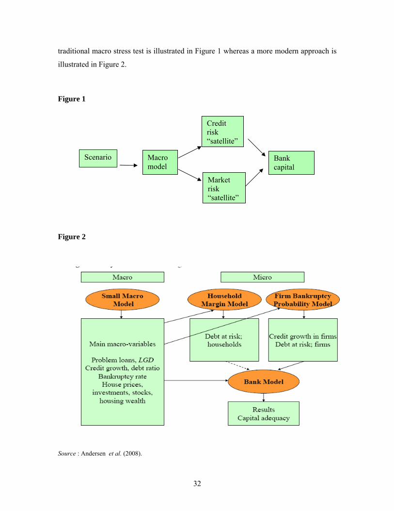
traditional macro stress test is illustrated in Figure 1 whereas a more modern approach is
illustrated in Figure 2.
Figure 1
Macro model
Market risk “satellite”
Credit risk “satellite”
Scenario Bank
capital
Figure 2
Source : Andersen et al. (2008).
32

The paper uses the traditional approach shown in Figure 1 and some traces of the
modern approach can be found in the effort to model the indirect credit risk effect.
However, direct interaction and feedback from the real economy (household and firms)
are ignored. Further, the model developed in the paper uses VAR (Vector
Autoregressive)4 techniques to create macroeconomic forecasts and focuses on the upper
leg of the figure, namely, on the credit ‘satellite’ model. Thus, the model can be
considered as part of a larger and more comprehensive macro stress testing framework.
However, the paper does not specify the purpose of the model. Macro stress
testing model can be used either for risk management purposes or financial stability
purposes. The former tries to investigate vulnerabilities of systemically important
financial institutions to adverse macroeconomic events and the latter common
vulnerabilities across institutions that could undermine the overall stability of the
financial system.
The second issue is the specification of the credit model. There are several
alternative specifications and the literature review of the paper analyses some important
contributions to the subject, namely the paper by Foglia (2009). The macroeconomic
variables to be considered in a macro stress test include: domestic variables (short-term
and long-term interest rates, inflation, GDP and unemployment) and external variables
(external demand, foreign interest rates, exchange rate fluctuations, etc.). The model by
Shijaku and Ceca uses three variables: GDP, interest rates, exchange rates and some
dummy variables.
Focusing on credit risk, the key parameters are basically the probability of default
(PD), the loss given default (LGD) and the exposure at default (EAD). Most models
focus on PD by increasing it by a predetermined amount, implying the credit quality of
all borrowers is worsened by some risk categories (downgrading). The customary
procedure for LGD and EAD is to assume an ad hoc increase by a given percentage or to
define some kind of range of variation and use it to calculate the change in credit risk.
The model here uses a proxy for the PD (non-performing loans) due to lack of data for 4 More sophisticated approaches use DSGE (Dynamic Stochastic General Equilibrium) modelling. See, Jokivuolle Ε., J. Kilponen and T. Kuusi (2007).
33
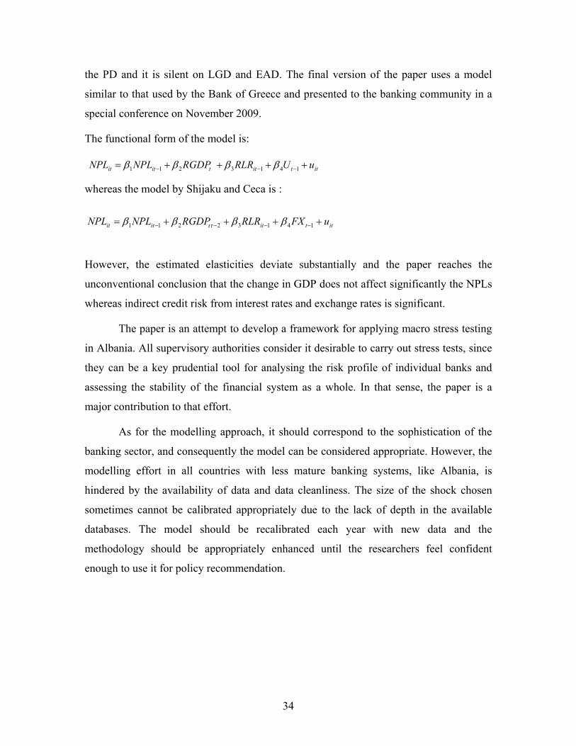
the PD and it is silent on LGD and EAD. The final version of the paper uses a model
similar to that used by the Bank of Greece and presented to the banking community in a
special conference on November 2009.
The functional form of the model is:
NPL
whereas the model by Shijaku and Ceca is :
NPL
ittittitit uURLRRGDPNPL ++++= −−− 1413211 ββββ
++++= −−−− 14132211 ββββ ιτ ittititit uFXRLRRGDPNPL
However, the estimated elasticities deviate substantially and the paper reaches the
unconventional conclusion that the change in GDP does not affect significantly the NPLs
whereas indirect credit risk from interest rates and exchange rates is significant.
The paper is an attempt to develop a framework for applying macro stress testing
in Albania. All supervisory authorities consider it desirable to carry out stress tests, since
they can be a key prudential tool for analysing the risk profile of individual banks and
assessing the stability of the financial system as a whole. In that sense, the paper is a
major contribution to that effort.
As for the modelling approach, it should correspond to the sophistication of the
banking sector, and consequently the model can be considered appropriate. However, the
modelling effort in all countries with less mature banking systems, like Albania, is
hindered by the availability of data and data cleanliness. The size of the shock chosen
sometimes cannot be calibrated appropriately due to the lack of depth in the available
databases. The model should be recalibrated each year with new data and the
methodology should be appropriately enhanced until the researchers feel confident
enough to use it for policy recommendation.
34

References
Andersen H., T. Berge, E. Bernhardsen, Ki-G. Lindquist and B.H. Vatne (2008), ‘A Suite-of-models Aproach to Stress-testing Financial Stability’, Norges Bank Financial Stability, Staff memo 2008/2.
Foglia, A. (2009), ‘Stress Testing Credit Risk: A Survey of Authorities’ Approaches,’ International Journal of Central Banking, 5, 9-45.
Jokivuolle Ε, J. Kilponen and T. Kuusi (2007), ‘GDP at Risk in a DSGE Model: an application to banking sector stress testing’, Bank of Finland Research Discussion Papers 26.
Rodrigo A. and M. Drehmann (2009), ‘Macro Stress Tests and Crises: what can we learn?”, BIS Quarterly Review, December.
35

36

Special Conference Papers
3rd South-Eastern European Economic Research Workshop Bank of Albania-Bank of Greece
Athens, 19-21 November 2009
1. Hardouvelis, Gikas, Keynote address: “The World after the Crisis: S.E.E. Challenges & Prospects”, February 2011.
2. Tanku, Altin “Another View of Money Demand and Black Market Premium Relationship: What Can They Say About Credibility?”, February 2011.
3. Kota, Vasilika “The Persistence of Inflation in Albania”, including discussion by Sophia Lazaretou, February 2011.
4. Kodra, Oriela “Estimation of Weights for the Monetary Conditions Index in Albania”, including discussion by Michael Loufir, February 2011.
5. Pisha, Arta “Eurozone Indices: A New Model for Measuring Central Bank Independence”, including discussion by Eugenie Garganas, February 2011.
6. Kapopoulos, Panayotis and Sophia Lazaretou “International Banking and Sovereign Risk Calculus: the Experience of the Greek Banks in SEE”, including discussion by Panagiotis Chronis, February 2011.
7. Shijaku, Hilda and Kliti Ceca “A Credit Risk Model for Albania” including discussion by Faidon Kalfaoglou, February 2011.
8. Kalluci, Irini “Analysis of the Albanian Banking System in a Risk-Performance Framework”, February 2011.
9. Georgievska, Ljupka, Rilind Kabashi, Nora Manova-Trajkovska, Ana Mitreska, Mihajlo Vaskov “Determinants of Lending Rates and Interest Rate Spreads”, including discussion by Heather D. Gibson, February 2011.
10. Kristo, Elsa “Being Aware of Fraud Risk”, including discussion by Elsida Orhan, February 2011.
11. Malakhova, Tatiana “The Probability of Default: a Sectoral Assessment", including discussion by Vassiliki Zakka, February 2011.
12. Luçi, Erjon and Ilir Vika “The Equilibrium Real Exchange Rate of Lek Vis-À-Vis Euro: Is It Much Misaligned?”, including discussion by Dimitrios Maroulis, February 2011.
13. Dapontas, Dimitrios “Currency Crises: The Case of Hungary (2008-2009) Using Two Stage Least Squares”, including discussion by Claire Giordano, February 2011.
37