A Cross-Sectional and Time-Series Analysis of Household

Consumption and a Forecast of Personal Consumption

Expenditures

Chang-yu I. Chao, Doctor of Philosophy, 1991

Dissertation directed by: Clopper Almon, Jr.Professor of Economics Department of Economics

ABSTRACT

T itle o f D isserta tion: A Cross-Sectional and Tim e-Series A nalysis o f HouseholdConsum ption and a Forecast o f Personal Consum ption Expenditures

Chang-yu I. Chao, D octor o f Philosophy, 1991

D isserta tion directed by: C lopper Alm on, J r.Professor o f Econom ics D epartm ent o f Econom ics

A system o f demand functions was developed to forecast personal

consum ption expenditures in 78 sectors fo r use in a long-term in p u t-o u t forecasting

m odel o f the U.S. economy. The equations incorporate the effects o f changes in

incom e, prices, and dem ographic factors. The influences o f incom e and household

characteristics on consum ption were estim ated in the cross-section. The effects o f

changing prices and trends were accessed in the tim e series.

The cross-section consum ption fu n ctio n was applied to the data obtained

from the Consum er Expenditures Survey. The household demand fo r a p a rticu la r

good is made up o f the product o f tw o com ponents: consum ption per household

m ember, and the specific size o f the household fo r th a t good. The expenditure per

household m ember is determ ined by household per capita incom e and dem ographic

a ttrib u te s o f households. The incom e-expenditure re la tionsh ip is expressed by a

Piecewise L inear Engel Curve (PLEC) fo r each o f the 61 cross-section consum ption

item s. A PLEC is capable o f representing luxu ries, necessities, as w e ll as in fe rio r

goods. It is also able to express d iffe ren t slopes fo r the Engel curve over d iffe ren t

incom e levels fo r a p a rticu la r good.

The product-specific size o f household was developed by the scheme o f adu lt

equivalency weights. The specific size o f a household is a weighted sum o f the

num ber o f household members In each age group, w ith w eights being the relevant

m agnitude, o r "a d u lt equivalent", fo r th a t age group fo r the given consum ption item .

The cross-section resu lts were transform ed in to tw o variab les, weighted

popu la tion and "cross-section-param eter" p red iction , fo r use in the estim ation o f tim e

series equations. W eighted populations were created by com bining the adu lt

equivalency w eights w ith popula tion to ta ls by age. "P redictions" were found by

com bining the cross-section Engel curves and dem ographic com position param eters

w ith incom e d is trib u tio n s and dem ographic popula tion proportions.

F in a lly , the system o f equations com bines the cross-section resu lts and the

price effects based on A lm on system . The equations were estim ated fo r 78

com ponents o f the N ational Income and Product Account’s Personal Consum ption

Expenditures over the 1966-1987 period. Forecasts o f consum ption were made

th rough the year 2000.

A CROSS-SECTIONAL AND TIME-SERIES ANALYSIS OF

HOUSEHOLD CONSUMPTION AND

A FORECAST OF PERSONAL CONSUMPTION EXPENDITURES

by

Chang-yu I. Chao

D isserta tion subm itted to the Facu lty o f the G raduate School o f The U n iversity o f M aryland in p a rtia l fu lfillm e n t

o f the requirem ents fo r the degree o f D octor o f Philosophy

1991

Advisory Com m ittee:

Professor C lopper A lm on, C hairm an/A dvisor Professor H arry K elejlan Professor F rank B rechling Professor Ed M ontgom ery Professor Rachel D ardis

ACKNOWLEDGEMENTS

I w ould like to th a n k Professor C lopper A lm on fo r h is invaluable guidance, encouragem ent and patience. I m ust thank m y parents, I. Chiou and Tsun Huang Chao, who have been extrem ely considerate and supportive th roughout every step o f m y grow th and education. I am also th a n k fu l to m y supervisor. Bob K irchner, who has been very encouraging fo r the com pletion o f m y d isserta tion. F in a lly , I have to th a n k m y husband, Der-Chau Song, fo r h is trem endous support and carefulness.

11

TABLE OF CONTENTS

C hapter 1 In tro d u ctio n 1

C hapter 2 Cross-Section Consum ption Functions 26I. The S tructu re o f Cross-Section C onsum ption Functions 27

A. Incom e vs. Consum ption Expenditures 29B. Household C haracteristics 33C. ,rB lg-T lcket"t Seldom -Bought Item s 41

II. D ata and E stim ation Scheme 47A. Data 47B. E stim ation Scheme 51

m . E stim ation R esults o f Least Squares M ethod 53A. O bservations on Engel Curves 53B. Im pact o f Dem ographic Variables 57C. O bservations on A d u lt Equivalency W eights 59

IV . E stim ation R esults o f the "B ig-T icket" Item s 61

C hapter 3 Incom e D is trib u tio n M odel and Tax System- A T ransition from Cross-Section to Tim e Series 126

I. D is trib u tio n o f Incom e 130A. The M odel 130B. D ata and E stim ation Procedure 137C. Forecasting the Income D is trib u tio n 140

n . Incom e Tax M odel 144III. D is trib u tio n o f D isposable Income 148

A . A djustm ent between AGI and PI 148B. D is trib u tio n o f D isposable PI 154

C hapter 4 Tim e-Series C onsum ption Functions 185I. A System o f Consum ption Functions 186

A . The System 186B. Incom e and Price E lastic itie s 195C. C reating "Cross-Section-Param eter P redictions" and

W eighted Populations 197D. Incorporating the Cross-Section Variables 202

II. E stim ation and Data 204A . E stim ation Procedure 204B. D ata 205

III. R esults 211A . Incom e E lastic itie s 211B. Price E lastic itie s 216C. Estim ates o f Non-Price Param eters 228

i l l

TABLE OF CONTENTS (C ontinued)

C hapter 5 Forecasting Personal Consum ption Expenditures 236I. Forecasts o f Personal Consum ption Expenditures 236

A . Forecasting Personal Consum ption Expenditures in theLIFT M odel 237

B. Forecast Assum ptions 239II. R esults - Forecast to 2000 240

A. Im pacts o f Incom e, Price, and Non-Price Factors 242B. P lots o f the Forecasts 243C. O utlook 258D . C onclusion 262

Appendix A 276

Appendix B 279

Appendix C 280

Appendix D 284

Selected B ib liography 289

iv

LIST OF TABLES

1.1 Cross-Section Consum ption Item s 31.2 N um erical Exam ple fo r a PLEC 61.3 W eighted Household Sizes fo r Four Typical Households 101.4 Tim e-Series Sectors 191.5 Population and Income D is trib u tio n by V entile and Household

Size - 1982 211.6 Upper L im its o f Per C apita AGI 221.7 Index o f V entile L im its fo r AGI 231.8 Index o f V entile L im its fo r Personal Income 241.9 Index o f V entile L im its fo r D isposable Personal Incom e 252.1 Cross-Section C onsum ption Categories 492.2 E stim ated C oefficients by Least Squares 632.3 E ffect o f Dem ographic Variables 732.4 Estim ated C oefficients by the B ig-T icket-Item A nalysis 963.1 E stim ation R esults fo r Param eters A and B 1573.2 H is to rica l Values o f E xplanatory Variables 1603.3 Tim e-Series Regression R esults o f Functiona l Param eters fo r

Each Household Size 1613.4 Regression E quation fo r Forecasting Tota l Exem ptions

(Num ber o f Exem ptions O ther Than Age o r B lindness) 1623.5 R esults o f Forecasting the Share o f T ota l P opulation fo r

Each o f the Household Size Categories 1633.6 R esults o f Forecasting the Share o f Total AGI fo r

Each o f the Household Size Categories 1693.7 P opulation and Income D is trib u tio n by V entile and Household

Size - 1982 1753.8 The D is trib u tio n o f C u to ff Per Capita AGI in C urrent D ollars

fo r Selected Years 1763.9 The D is trib u tio n o f CutofTPer C apita AGI Relative to Average

AGI fo r Selected Years 1773.10 E ffective and Standard Tax Rates 1783.11 R atios o f E ffective-to-S tandard Tax Rates 1793.12 The Twelve R econcilia tion Item s vs. the NIPA Tables 1803.13 E stim ation R esults fo r the R econcilia tion Item s 1813.14 The D is trib u tio n o f R econcilia tion Item s between AGI and PI 1833.15 Index o f V entile L im its fo r Personal Income 1844.1 Tim e-Series Consum ption Item s 2074.2 The Correspondence between the Cross-Section and the

Tim e-Series Sectors 2094.3 Incom e E lastic itie s 2134.4 Price E lastic itie s 2224.5 Estim ates o f Non-Price Param eters 2315.1 Assum ptions o f Econom ic Variables and Dem ographic

Com positions 2415.2 Forecast o f Consum ption (M illions o f 1982 D ollars) 2645.3 G row th Rates (Percent) 270

v

LIST OF FIGURES

1.1 A Piecewise Linear Engel Curve 51.2 B ar C hart o f A d u lt Equivalency W eights 112.1 A Piecewise Linear Engel Curve 312.2 P lot o f Engel Curves 762.3 B ar C hart o f A d u lt Equivalency W eights 863.1 Flow C hart o f Income D is trib u tio n and Tax M odels 1293.2 The Lorenz Curve Transform ation 1313.3 T & S fo r 1981 Household Size One 1353.4 (S**1.5)*((V2-S)**.5) P lotted on S 1353.5 S & T w ith D iffe ring Values o f A and B

- 1981 Household Size One 1363.6 S & T w ith D iffe ring Values o f A and B

- 1981 Household Size One 1363.7 Tim e Series o f A and B-1981 Household Size Three 1393.8 NIPA Table 3.11 1513.9 NIPA Table 8.14 1524.1 The G rouping Scheme 1944.2 W eighted Population 2005.1 P lots o f the Forecasts 2455.2 Personal C onsum ption Expenditures

- A nnual G row th Rates (%) 2585.3 A uto and Auto-Related Consum er Spending

- A nnual G row th Rates (%) 2605.4 The C om position o f PCE 261

v i

CHAPTER 1

INTRODUCTION

The size and com position o f the economy’s to ta l ou tpu t depend heavily upon

the size and com position o f consum er expenditures. W ith a share o f approxim ately

s ix ty-five percent, personal consum ption expenditure is the largest com ponent o f the

U.S. Gross N ational Product. Changes in consum ption patterns w ill therefore

strong ly in fluence changes in o ther economic a ctiv itie s lik e p roduction, em ploym ent,

and investm ent. Consequently, a proper forecast o f personal consum ption

expenditures Is necessary to explain o r p red ict the other c ru c ia l econom ic activ ities.

A com prehensive demand analysis m ust incorporate an Investigation in to

the effects o f changes in incom e, prices, and dem ographic facto rs. This is the goal

o f the m odel described In th is d isserta tion. M oreover, the m odel is to be used to

forecast personal consum ption expenditures in a long-term in p u t-o u t forecasting

m odel o f the U.S. economy developed by the In te rin d u s try Forecasting Project a t the

U n iversity o f M aryland (Inforum ).

O ur fo rm u la tion o f the com prehensive demand m odel begins w ith b u ild ing

a consum ption fu n ctio n to be estim ated from cross-section data on the purchases

o f m any households. The In fo rm ation acquired from the cross-section is to be used

to expla in the tim e-series consum ption behavior. More precisely, the cross-section

Is used to id e n tify the effects o f Income and household characteristics, w h ile the tim e

series is used to assess the effects o f changing prices and trends no t accounted fo r

by any o f the variab les in the cross-section. The cross-section consum ption function

developed here is applied to the data obtained from the Consum er Expenditures

Survey (CES) conducted by the Bureau o f Labor S ta tis tics (BLS). The w ide varie ty

o f households in the BLS sample allow s cross-section data to provide a ric h d ive rsity

1

o f incom e, expenses, and dem ographic a ttrib u te s o f households. Each household in

the sam ple provides in fo rm ation concerning its incom e, purchases o f d iffe ren t

products, age o f household head, education, occupation, region o f residence, num ber

o f earners, and fam ily size.

The household demand fo r a p a rticu la r good is made up o f the product o f

tw o com ponents: consum ption per household member; and the specific size o f the

household fo r th a t good. The expenditure per household member is determ ined by

household per capita incom e and dem ographic a ttrib u te s o f households. The specific

size o f a household is a weighted sum o f the num ber o f household members in each

age group, w ith the w eights being the relevant m agnitude, o r "adu lt equivalent", fo r

th a t age group fo r the given consum ption item . T h is is know n as the scheme o f adu lt

equivalency w eights. The reference "a d u lt” is defined in th is m odel to be an adu lt

between th irty -o n e and fo rty years o f age.

The firs t step in constructing the com ponent o f per cap ita household

consum ption is to establish a flexib le form o f Engel curve. A n Engel curve represents

an incom e-expenditure re la tionsh ip . I t p lo ts the consum ption expenditure on a

com m odity against the incom e o f consum ers. A flex ib le Engel functiona l form should

be able to represent lu xu ries, necessities, as w e ll as in fe rio r goods. M oreover, it

shou ld be capable o f expressing d iffe ren t slopes fo r the Engel curve over d iffe ren t

incom e levels fo r a p a rticu la r good. In o ther words, it is possible th a t a given

com m odity is a necessity fo r one incom e group w h ile being a lu xu ry (or an in fe rio r

good) fo r another.

Table 1.1 contains a com plete lis tin g o f the 61 consum ption item s to be

investigated.

2

TABLE 1.1

Cross-Section C onsum ption Item s

1. Food, o ff prem ise2. Food, on prem ise3. A lcoholic beverages, o ff prem ise4. A lcoho lic beverages, on prem ise5. Tobacco products6. Shoes and footwear7. W omen's and ch ild ren ’s c lo th ing8. Men’s and bey’s c lo th ing9. Luggage10. Jew elry and watches11. Laundries, storage, and repa ir o f c lo th ing and shoes12. O ther jew elxy and clo th ing services13. Personal care14. O wner-occupied housing15. Tenant-occupied housing16. O ther housing17. A dd itions, a lte ra tions, and constructions o f residencies18. H otels and m otels19. F u rn itu re20. K itchen and household appliances21. C hina, glassware, and tableware22. O ther durable house fu rn ish ings23. F loor coverings24. Sem idurable house fu rn ish ings25. E le c tric ity26. N a tu ra l gas27. Fuel o il and coal28. W ood, other fu e l, and bottled o f ta n k gas29. W ater and other san ita ry services30. Telephone and telegraph31. Dom estic service32. O ther household operations33. Household Insurance34. P rescrip tion drug and sundries35. Physicians36. D ental and eyes37. O ther m edical services and supplies38. H ospita ls and san ita rium s39. H ealth Insurance40. Personal business41. L ife insurance42. New cars43. Used cars44. New and used tru cks o r vans45. T ires and tubes46. A u to accessories and parts

3

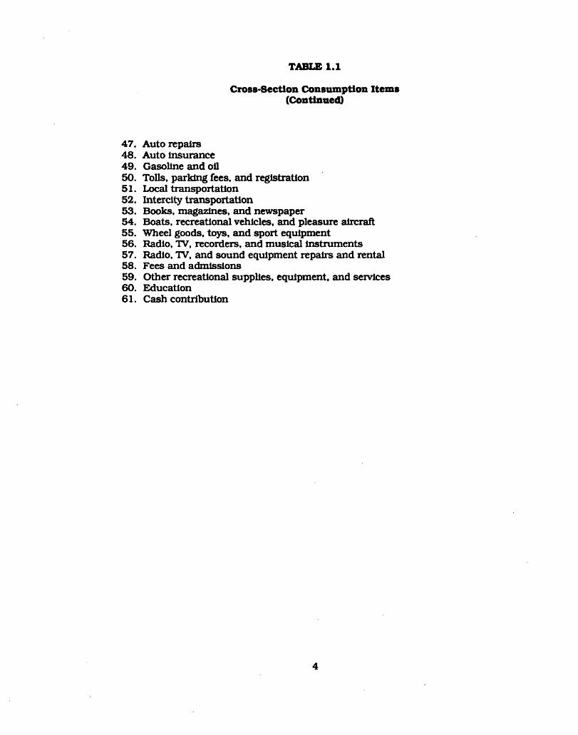
Cross-Section C onsum ption Item s (C ontinued)

TABLE 1.1

47. A uto repairs48. A uto insurance49. G asoline and o il50. T o lls, parking fees, and reg is tra tion51. Local tran spo rta tio n52. In te rc ity tran spo rta tio n53. Books, m agazines, and newspaper54. Boats, recreationa l vehicles, and pleasure a irc ra ft55. W heel goods, toys, and sport equipm ent56. Radio, TV, recorders, and m usical instrum ents57. Radio, IV , and sound equipm ent repairs and ren ta l58. Fees and adm issions59. O ther recreationa l supplies, equipm ent, and services60. E ducation61. Cash co n trib u tio n

4

The* Engel re la tionsh ip in th is d isserta tion accounts fo r the effect o f per

cap ita household Income on per capita household expenditure. In order to form ulate

th is flex ib le form , per cap ita household Income Is divided in to a num ber o f Income

brackets, in th is case five . The boundaries o f the five incom e brackets are

determ ined such th a t each o f the five brackets contains exactly one fifth o f the to ta l

households in the sam ple. Therefore, the Engel curve fo r a given consum ption item

is lin e a r in each o f the brackets b u t w ith d iffe ren t slopes in d iffe ren t brackets. This

form is called the Piecewise L inear Engel Curve (PLEC). F igure 1.1 depicts a PLEC

w ith five incom e brackets. The num erica l example in Table 1.2 can help to illu s tra te

th is five-incom e-bracket PLEC.

FIGURE 1.1

A Piecewise L inear Engel Curve

$0 $2,000 $4,000 $6,000 $8,000 $10,000 $12,000NC0ME

5

TABLE 1.2

N um erical Exam ple fo r a PLEC

Amount o f Income i n B ra c k e t

H ouseho ld H ouseho ldIncome 1 2 3 4 5

A 1,500 1 ,500 0 0 0 0

B 3 ,500 3 ,000 500 0 0 0

C 5 ,50 0 3 ,000 2 ,000 500 0 0

D 6,500 3 ,000 2 ,00 0 1 ,000 500 0

E 11,000 3 ,000 2 ,00 0 1 ,000 3 ,000 2 ,00 0

B o u n d a r ie s o f B0: Income B ra c k e t $0

Bx: $3 ,000

B2 :$5 ,000

B3:$6 ,000 * B<: $9 ,000

B5:I n f i n i t y

6

The advantage o f a PLEC can be h igh ligh ted by its a b ility to adequately

express the characteristics o f a typ ica l consum ption product. For exam ple, rich

households are lik e ly to have a h igher m arg ina l propensity to consume (MPC)

lu xu rie s than are poor households. The slope o f the PLEC fo r th is item , thus, w ill

be steeper In the h igher incom e levels w h ile being m oderate in the low er Income

brackets. On the o ther hand, the PLEC w ill illu s tra te a lin e a r curve w ith a re la tive ly

constant slope i f the MPC fo r a good is rough ly the same over the five incom e

brackets.

The second step in m odeling is Incorporating dem ographic factors in to

household consum ption. The m odel classifies the household characteristics in to five

categories. They are: region o f residence, education o f household head, w orking

sta tus o f spouse, fam ily size, and age o f household head. The dem ographic

characte ristics o f households m ay affect household spending on various

consum ption item s to a varying extent. The fo llow ing exam ples m ay account fo r the

relevance o f these dem ographic variab les in the household consum ption:

Region:

The difference in clim ate resu lts In greater expenditure on

heating u tilitie s fo r households In the northeast over those in the

south. O n the o ther hand, the households in the west have a

re la tive ly large num ber o f renters whose u tilitie s are included in ren t.

Thus, these households spend less on e le c tric ity , gas, and w ater b u t

m ore on shelter than households in o ther regions.

E ducation:

The education level o f the household head affects the

7

household expenditures especially on ch ild ren 's education and

reading m ateria ls. A household w ith a college-educated head m ay

spend m ore on education related Item s than a household w ith o u t a

college-educated head.

W orking Spouses:

The dram atic increase In the p a rtic ip a tio n o f women in the

labor force leads to the greatest change in recent household

consum ption patterns. In the 1950's, less th a n 20 percent o f women

were wage earners. T h is p a rtic ip a tio n m ore than doubled, however,

in the 1970’s. W orking w ives spend less tim e on housework than do

fu ll-tim e housem akers. Therefore, tw o-eam er households should

tend to spend a re la tive ly large am ount on tim e-saving item s like

dom estic and household services.

Fam ily Size:

Fam ily size is im portan t in in te rp re tin g economies o f scale.

A n increase In household size Inversely affects the household

consum ption on luxu ries. The household consum ption on necessities

and in fe rio r goods, on the o ther hand, w ill go up w ith an increase in

household size.

Age:

The m iddle aged household head w ill tend to spend a

re la tive ly large am ount on transpo rta tion and personal business. In

con trast, e lderly people tend to spend a h igher p o rtio n o f th e ir income

8

on hea lth care.

The procedure o f in c lud ing dem ographic facto rs In the PLEC is to allow only

the In te rcept o f the PLEC to be d iffe ren t fo r each dem ographic group. In o ther words,

the effect o f dem ographic variab les s h ift th e . en tire Engel curve upw ards or

downwards in a pa ra lle l pa tte rn w ith o u t affecting the specific propensity to consume

o u t o f incom e. Th is task is accom plished by constructing a zero-one dum m y variab le

fo r each o f the dem ographic categories.

The next process is to provide the second com ponent o f household

consum ption, the product-specific size o f household, by developing a d u lt equivalency

w eights. The a d u lt equivalency w eights give each age group a d iffe ren t w eight in the

expenditure on each good. Thus, they perm it us to give h igh w eights to the group

o f consum ers who are lik e ly to consume a com m odity w h ile g iving re la tive ly low

w eights to those less lik e ly to consume the good.

A n example o f th is is shown in Table 1.3 using the consum ption o f alcohol,

fu rn itu re , and m edical care. The specific weighted household size fo r the

consum ption o f alcohol, fu rn itu re , and m edical care are shown In Table 1.3 fo r fou r

households w ith d iffe ren t age com positions. Each o f the fo u r households in Table

1.3 has fo u r fam ily m embers. The weighted household size fo r a given household,

however, d iffe rs from good to good. M oreover, the range o f weighted household size

fo r a p a rtic u la r good is ra th e r large. For exam ple, the fo u r m ember households

range in size from 2.6 to 6.0 fo r fu rn itu re . Figure 1.2 shows the estim ated adu lt

equivalency weights fo r O ff prem ise alcohol consum ption, F u rn itu re , and H ealth

insurance. They show p lausib le patterns broad ly s im ila r to the hypo the tica l ones in

Table 1.3. The pa tte rn fo r fu rn itu re is p a rticu la rly notew orthy.

9

W eighted Household Sizes fo r Four T yp ica l Households

TABLE 1.3

Number o f F a m i ly Members

H ouseho ld C h i l d r e n A d u l t s The Aged

A 2 2 0

B 1 3 0

C 1 2 1

D 0 2 2

A d u l tE q u iv a le n c yW e ig h ts

A l c o h o l 0 .1 1 .0 0 .5

F u r n i t u r e 2 .0 1 .0 0 .3

M e d ic a l Care 1 .5 1 .0 2 .0

W e igh te d H ouseho ld S iz e

A lc o h o l F u r n i t u r e M e d ic a l Care

2 .2 6 .0 5 .0

3 .1 5 .0 4 .5

2 .6 4 .3 5 .5

3 .0 2 .6 6 .0

10

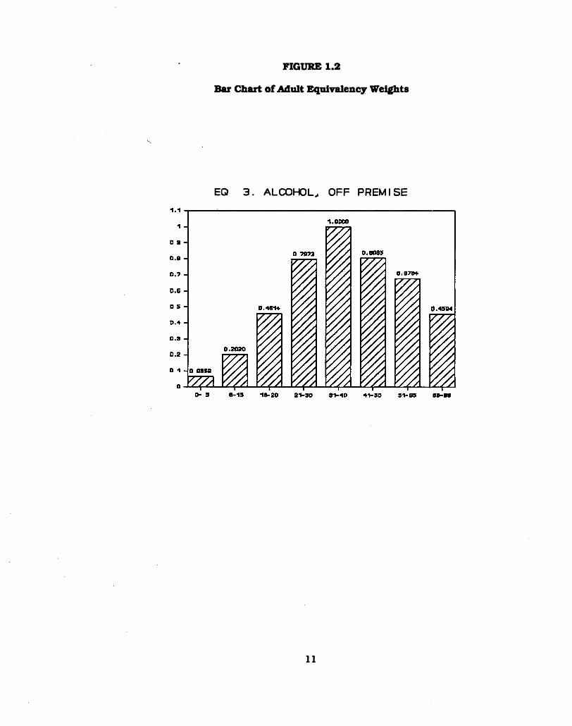
FIGURE 1.2

Bar C hart o f A d u lt Equivalency W eights

EQ 3 . ALCOHOL, OFF PREMI5E

11

Bar C hart o f A d u lt E quivalency W eights (C ontinued)

FIGURE 1.2

EQ 19 . FURNITURE

12

Bar C hart o f A d u lt E quivalency W eights (C ontinued)

FIGURE 1.2

EQ 3 9 . HEALTH INSURANCE

13

The second p a rt o f the com prehensive demand m odel is a system o f demand

equations in the tim e series. These equations incorporate the in fo rm ation inc lud ing

size d is trib u tio n o f incom e, age s tructu re o f popula tion, dem ographic com position,

and re la tive prices. The system estim ates 78 com ponents o f U.S. personal

consum ption expenditures in the N ational Incom e and Product Accounts. A

com plete lis t o f 78 sectors Is shown in Table 1.4.

In the process o f estim ating th is system , a tim e-series o f weighted

popula tions is firs t created fo r each consum ption item by using the a d u lt equivalency

w eights. The popula tion to ta ls fo r each o f the e ight age groups are obtained from the

C urren t P opulation Reports published by the Census Bureau. The com m odity

specific weighted populations are com puted by sum m ing the num ber o f ind iv idua ls

In each age group weighted by the corresponding equivalency w eight o f a given good

over a ll the age groups. The weighted populations are calculated fo r each o f the 78

categories shown in Table 1.4.

The advantage o f using weighted popula tions as opposed to using sim ple

popu la tion to ta ls is the a b ility to re flect sh ifts in demand as the age s tru c tu re o f the

popu la tion changes. For Instance, the cross-section resu lts show th a t young

ch ild ren have a re la tive ly h igh adu lt equivalency w eight In fu rn itu re . The weighted

popu la tion fo r fu rn itu re , therefore, w ill grow ra p id ly as the size o f 0-5 age group

grows. However, the popula tion grow th In th is group w ill no t affect the weighted size

o f popu la tion fo r alcohol because they con tribu te alm ost no th ing to alcohol

consum ption.

The estim ated cross-section param eters are then used in con junction w ith

in fo rm a tion on size d is trib u tio n o f income and dem ographic com position to create a

"p red iction" o f per a d u lt equivalent expenditure fo r each good. The "pred iction"

w h ich is com prised o f tw o com ponents, income and dem ographic sh ifts , w ill be used

14

as an explanatory variab le in the tim e-series consum ption function . In o ther words,

th rough the use o f "pred ictions", we have assumed th a t on ly the facto rs considered

in the cross-section affect consum ption in the tim e series and the param eters

estim ated in the cross-section accurately re flect those influences.

The m agnitude o f the dem ographic s h ift com ponent o f the "pred ictions" is

calculated by sum m ing over the population proportion fo r each dem ographic category

in a given year weighted by the corresponding cross-section coefficient. Namely, th is

aggregation procedure gives the m ost w eight to the m ost relevant variab les fo r a

specific good. For example, the geographic regions are no t h e lp fu l in the cross-

section equation fo r dom estic services, because a s h ift in the m igra tion o f the

popu la tion does no t greatly influence the value o f the "predictions" fo r dom estic

services. However, a s h ift in the num ber o f w orking spouses should greatly affect the

consum ption o f th is good.

In order to calculate the incom e com ponent o f the "pred ictions", it is

necessary to know the de ta ils o f the d is trib u tio n o f incom e. The PLEC is very

sensitive to the d is trib u tio n o f Income because it is based on the five segments

defined by household Income. Recall th a t the cross-section incom e variab les are the

am ount o f incom e received by one fam ily m em ber w ith in a specific incom e bracket.

Thus, In the tim e series, the average values o f these five incom e variab les have to be

com puted fo r each year. To calculate the m agnitude o f incom e variab le fo r a given

Income bracket, the am ount o f incom e received by each person In th a t bracket is

aggregated, and then the sum o f Income w ith in the bracket is divided by the to ta l

num ber o f ind iv idua ls.

The basic idea o f ou r incom e d is trib u tio n m odel is to convert the m odel’s

forecasts o f aggregate personal incom e in to a detailed d is trib u tio n o f AG I. The firs t

step o f m odeling, therefore, is to ob ta in a forecast o f the size d is trib u tio n o f incom e.

15

The Income d is trib u tio n in th is d isserta tion is represented by a Lorenz curve. A

Lorenz curve p lo ts the percentages o f popula tion on the horizon ta l axis against the

percentages o f incom e they receive on the ve rtica l axis. The data u tilize d fo r

estim ating a Lorenz curve is the grouped data on the d is trib u tio n o f adjusted gross

incom e (AGI) from S ta tis tics o f Incom e (SOI), published by the In te rn a l Revenue

Service. The shape o f each Lorenz curve is described by two param eters: the

am ount by w hich each curve bows away from the diagonal lin e o f equally d is tribu te d

incom e re la tive to the base year’s (1981) curve; and the am ount by w hich each curve

is skewed tow ard e ithe r the upper o r low er end o f the d is trib u tio n re la tive to the base

year's curve. The two param eters are estim ated fo r each year and each household

size. For the purpose o f forecasts, these estim ated Lorenz curve param eters are

arranged in tim e-series, and are regressed on cyclica l econom ic variab les and a tim e

trend. Consequently, these estim ated equations are used in con junction w ith the

forecasts o f the cyclica l econom ic variables to forecast the Lorenz curves. The

forecasts o f the cyclica l econom ic variables come from the m acro m odel. The

re su ltin g Lorenz curves are then applied to the aggregate AG I, w hich is forecast as

a fu n c tio n o f personal income and item s like tran sfe r paym ents.

The d is trib u tio n o f AGI and the SOI data are then used to develop the tax

m odel. The objective o f the ta x m odel is to remove incom e taxes from household

incom e and to get a d is trib u tio n o f per capita disposable incom e to be used in the

consum ption functions. O ur consum ption functions require a d is trib u tio n o f

personal incom e w hich groups the popula tion in to ventiles. Each ventile contains

five percent o f the popula tion. Furtherm ore, it is necessary to calculate the tax rate

schedules separately fo r d iffe ren t household sizes because incom e taxes are levied

on the basis o f household incom e.

Table 1.5 shows the d is trib u tio n o f popula tion by ca lcu la ting the num ber

16

o f fam ilies o f each household size fo r each incom e group and the d is trib u tio n o f AGI

among the s ix household sizes and the tw enty incom e groups. W ith in ventlles.

Ind iv idua ls are arranged In ascending order. The Income d is trib u tio n , thus, is

defined by indexes w hich represent the Income o f the h ighest person in each ventile

re la tive to the overall average per capita Income. Table 1.6 shows the upper lim it o f

per cap ita AG I In each ventile . Table 1.7 shows the values o f the upper lim its o f per

cap ita AGI re la tive to the overall m ean per capita AG I.

In fa c t. I t is the d is trib u tio n o f disposable personal incom e, no t AG I, w hich

determ ines consum ption in ou r m odel. Thus, the d is trib u tio n o f AGI needs to be

transform ed in to the d is trib u tio n o f disposable incom e. The transform ation is

accom plished through a bridge w hich d is trib u te s the item s no t p a rt o f AGI among

the ventlles. These item s include tran sfe r paym ents, fringe benefits. Im putations,

and o ther types o f incom e. The index o f ventile lim its fo r personal incom e is shown

In Table 1.8.

In the tax m odel, there are a to ta l o f 120 tax rates fo r tw enty incom e groups

and s ix household sizes. To apply the incom e and tax m odel to the consum ption

functions, however, we have to com bine the d is trib u tio n o f s ix household sizes in to

a single d is trib u tio n . Thus, the tax rates are aggregated in to a weighted-average

incom e ta x ra te o f s ix household sizes fo r each incom e group. The tax rates are then

applied to the d is trib u tio n o f AGI and personal incom e to get the d is trib u tio n o f both

disposable AG I and disposable personal incom e. Table 1.9 shows the indexes o f

ven tile lim its fo r disposable personal incom e w hich includes a forecast to the year

2000.The fin a l and the m ost c ru c ia l step in m odeling the system o f consum ption

functions is to exam ine the price effects. In ou r system o f demand equations, the

dem and fo r a good depends upon the prices o f a ll o ther goods. However, the price

17

effects are s im p lified by assum ing th a t consum ption item s w ith s im ila r economic

characte ristics can be com bined in to groups. Thus, through the grouping technique,

a com m odity can be a strong com plem ent o r substitu te fo r o ther item s in its own

group w h ile having less strong price in te ractions w ith goods in o ther groups.

M oreover, a group can be s p lit in to several subgroups. The construction o f

subgroups is to achieve even greater fle x ib ility fo r the price in te ractio n patterns. A

specific subgroup m ay conta in e ithe r com plem entary o r substitu tab le item s

independently o f the other subgroups. Therefore, it is possible fo r the goods in the

firs t subgroup to be substitu tes fo r the goods in the second subgroup w h ile being

com plem ents to those in the th ird .

The u ltim a te goal o f ou r consum ption m odel, w hich is an in teg ra l p a rt o f the

LIFT m odel, is to help the m odel’s a b ility to forecast the other econom ic a ctiv itie s like

production and investm ent. Thus, a proper forecast o f personal consum ption

expenditures is necessary. The pro jection o f consum ption has to be made

sim ultaneously w ith the determ ination o f prices and Income in the LIFT m odel. A

fin a l forecast o f personal consum ption expenditures is achieved through an Ite ra tive

process. The 78 com ponents o f U.S. personal consum ption expenditures are

projected to the year 2000.

Chapter 2 describes the m odel and the estim ation scheme fo r the cross-

section consum ption functions. C hapter 3 form s the tra n s itio n from the cross-

section to the tim e series. Chapter 4 describes the system o f demand equations in

the tim e series. C hapter 5 explains the procedures fo r forecasts by using the resu lts

obtained from the previous three chapters. A review o f em pirica l consum ption

functions is presented in Appendix A.

18

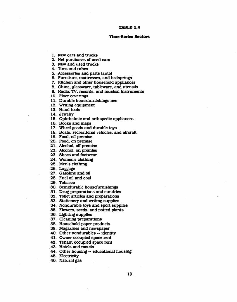
TABLE 1.4

Tim e-Series Sectors

1. New cars and tru cks2. Net purchases o f used cars3. New and used tru cks4. T ires and tubes5. Accessories and parts (auto)6. F u rn itu re , m attresses, and bedsprings7. K itchen and o ther household appliances8. C hina, glassware, tableware, and u tensils9. Radio, TV, records, and m usical instrum ents10. F loor coverings11. D urable housefum ishings nec12. W ritin g equipm ent13. Hand tools14. Jew elry15. O phthalm ic and orthopedic appliances16. Books and maps17. W heel goods and durable toys18. Boats, recreationa l vehicles, and a irc ra ft19. Food, o ff prem ise20. Food, on prem ise21. A lcohol, o ff prem ise22. A lcohol, on prem ise23. Shoes and footw ear24. Women’s clo th ing25. Men’s clo th ing26. Luggage27. Gasoline and o il28. Fuel o il and coal29. Tobacco30. Sem idurable housefum ishings31. D rug preparations and sundries32. T o ile t a rtic les and preparations33. S tationery and w ritin g supplies34. Nondurable toys and sport supplies35. Flowers, seeds, and potted p lan ts36. L igh ting supplies37. C leaning preparations38. Household paper products39. Magazines and newspaper40. O ther nondurables — id e n tity41. Owner occupied space re n t42. Tenant occupied space ren t43. H otels and m otels44. O ther housing — educational housing45. E le c tric ity46. N a tu ra l gas

19

TABLE 1.4

Tim e-Series Sectors (C ontinued)

47. W ater and o ther san ita ry services48. Telephone and telegraph49. Dom estic services50. Household insurance51. O ther household operations -- repa ir52. Postage53. A uto repa ir54. B ridge, to lls , etc.55. A u to insurance56. Taxicabs57. Local pub lic tran spo rt58. In te rc ity ra ilro ad59. In te rc ity buses60. A irlin e s61. Travel agents and o ther transpo rta tion services62. C leaning, laundering and shoe repa ir63. Barbershops and beauty shops64. Physicians65. D entists and other professional services66. P rivate hosp ita ls and san ita rium s67. H ealth Insurance68. Brokerage and Investm ent counseling69. B ank services charges and services w ith o u t paym ent70. L ife Insurance71. Legal services72. Funera l expenses and other personal business73. Radio and te levision repa ir74. M ovies, legitim ate theatre , and spectator sports75. O ther recreational services76. E ducation77. R eligious and w elfare services78. Foreign trave l

20

TABLE 1.5

P opulation and Incom e D is trib u tio n By V e n tile and Household Size - 1982

Exem ptions O th e r th a n Age o r B l in d n e s s i n Thousands

HouseholdV e n t i l e

1

S iz e 1 2 3 4 5 6 T o t a l

1886.4 1249.1 1674.8 2137.4 1521.6 2314.1 10783.52 2426 .0 1110.9 1350.3 1750.8 1549.6 2595.9 10783.53 1365.1 1130.2 1677.1 2465.4 1828.5 2317.1 10783.54 2363.5 1459.7 1821.8 2066.3 1464.3 1608.3 10783.85 973.7 1458.8 1665.5 2097 .9 1720.5 2867.4 10783.86 2018.1 1632.2 1524.7 2319.4 1358 .0 1931.4 10783.87 1037.8 1758.4 1609.3 2427.3 3282 .6 668 .6 10783.88 1728.3 1873.1 1746.7 1753.9 687 .0 2994 .9 10783.89 794.7 1234.9 1355.3 4105.4 2914 .9 3 78 .6 10783.8

10 1973.5 2513.1 2455.9 2593.0 688.1 559 .8 10783.511 1494 .6 1528.3 802.8 5172.3 959.4 826 .6 10783.812 1217.1 1798.0 3092.9 736.3 3640.3 299 .2 10783.813 2283.3 2835.7 2361.3 2138.5 753.2 411 .8 10783.714 1016.0 1329.4 1082.5 6129.6 1018.5 208 .0 10783.815 2844.5 2528.2 2845.7 1537.5 762.4 265 .2 10783.516 1367.8 3963.2 2492.3 2564.9 354 .2 4 0 .9 10783.517 2989.8 2688.6 3087.6 1254.8 656.6 106 .0 10783.518 3162.7 3499.1 2186.0 1598.6 170.2 166 .9 10783.519 3046.8 5844.3 913.9 453 .9 255 .0 269 .6 10783.520 3185.6 4208.3 1320.3 1271.3 589.1 209 .3 10783.8

T o t a l s 39175.2 45643.5 37066.7 46574.5 26174.2 21039 .5 215673.6

A d ju s te d Gross Income i n m i l l i o n s o f D o l l a r s

Househo ld S iz e 1 2 3 4 5 6 T o t a lv e n t i i e

i 1832.4 1300.8 1351.4 1726.9 1081.1 1755.8 9048.42 4155.2 1643.5 2196.2 2845.8 2451.8 4062.0 17354.53 2832.6 2529.7 3709.9 5433.7 4014.9 5077.5 23589.34 6770.3 4102.6 5044.4 5748.0 4102.2 4406.4 30173.95 3266.7 4901.9 5624.7 7076.6 5789.0 9534.0 36192.96 7856.3 6349.5 5919.3 9066.1 5168 .0 7797.0 42156.27 4661.5 7801.8 7175.2 10760.0 14903.3 2874 .5 48176.38 8534.1 9320.3 8754.0 8677.5 3410.5 15572.3 54268.79 4433.7 6849.4 7447.0 23327.8 16316.7 1992.8 60367.4

10 11905.2 15427.8 15122.1 15320.2 4159.0 3536.9 65471.211 10306.1 10448.4 5364.9 36281.3 6736.0 5611.2 74747.912 9135.1 13369.4 23850.9 5297.4 26118.4 2 087 .6 79858.813 18904.5 23620.0 18828.6 18465.5 6323.0 3520.8 89662.414 9273.3 12167.6 10205.1 54535.2 9349.3 1918.5 97449.015 29234.8 25610.4 27747.4 15973.0 7589.3 2531.1 108686.016 15800 .9 4 6263.4 29638.8 29453.6 4235.8 446 .0 125838.517 38938.8 36153.0 38044.3 16399.9 8229.4 1154.7 138921.118 50420.7 53890.9 33804.6 24577.3 2488.8 1818.6 167000.919 62936.3 111019.7 18407.4 7728.7 3728.7 6393.3 210213.520 124235.8 161632.7 45567.6 40552.8 19007.6 5699.5 396696.0

T o t a l s 425434.3 554402.8 313803.8 339247.3 155202.8 87790.5 1875881.5

21

TABLE 1.6

Upper Limits of Per Capita AGI

V e n t l i e 1966 1975 1982

1 455 .1 7 39 .6 1212.12 682.4 1136.1 1886.43 830 .8 1443.1 2 50 9 .54 9 90 .3 1780.3 3079 .05 1127.8 2088 .3 3628 .86 1283 .3 2392 .5 4 16 8 .07 1415.6 2694 .8 4 70 4 .28 1575.7 3040 .3 5 30 1 .89 1691.4 3322.8 5722 .4

10 1852.2 3553 .5 6 554 .511 2050.4 4070 .5 7131 .212 2246 .7 4 27 8 .6 7763 .313 2483 .2 4828 .2 8 88 3 .914 2751 .7 5196 .0 9463.115 3014.1 5907 .6 11111 .616 3516.4 6769.1 11987.017 3890.6 7816.2 14253 .718 4 839 .6 9672 .9 17823 .619 6538.3 12807.8 23171 .920 DO OO OO

22

TABLE 1.7

Index of Ventile lim its for AGI

V e n t i l e 1966 1975 1982

1 18.12 15.54 13.942 2 7 .1 7 2 3 .8 7 2 1 .6 93 33 .08 30 .32 2 8 .8 54 39.44 37 .40 3 5 .4 05 4 4 .9 1 43 .87 4 1 .7 26 51 .10 5 0 .2 6 4 7 .9 27 5 6 .37 5 6 .61 5 4 .0 88 62 .75 63 .87 60 .969 6 7 .36 69.81 65 .79

10 7 3 .7 6 7 4 .65 7 5 .3 611 81 .65 85 .51 8 1 .9 912 89 .47 89 .88 8 9 .2613 98 .89 101 .43 102.1414 109 .58 109 .16 108 .8015 1 20 .03 124.11 127 .7516 140 .03 142 .21 137 .8217 154 .93 164.20 163 .8818 192 .73 203 .21 204 .9219 260 .37 269 .07 266 .4120* 20 .65 19 .69 2 1 .1 5

Average AGI 251 1 .1 3 4760.04 8697 .75

*The o v e r a l l p e rc e n ta g e o f t h e t o t a l income h e ld by t h e r i c h e s t 5% o f p o p u la t io n

23

Index o f V e n tile L im its fo r Personal Incom e

TABLE 1.8

V e n t i l e 1966 1975 1982

1 14 .49 16 .58 15.942 18 .37 2 6 .4 0 2 5 .7 93 3 3 .90 4 3 .9 6 4 2 .6 94 40 .48 49.04 4 8 .2 15 4 6 .4 5 5 3 .9 2 5 2 .8 96 5 1 .7 5 58 .22 5 7 .0 37 57 .90 63.04 61 .698 63.20 67 .86 66 .499 68 .93 73 .02 7 1 .1 3

10 73 .80 7 7 .99 75 .8111 8 0 .45 8 3 .35 82 .8712 88.04 90 .17 88 .4013 97.09 97 .48 97 .7214 108 .00 107 .01 107 .3215 119 .57 118 .87 120 .7016 137.94 136 .36 133 .8617 156.11 158.98 157 .2318 192 .42 195 .66 195 .8919 2 59 .03 2 59 .97 2 55 .7020* 2 0 .99 19 .35 2 0 .5 3

Average 3055 .69 6081.14 11483.39p i

"The o v e r a l l p e rc e n ta g e o f t h e t o t a l Income h e ld by t h e r i c h e s t 5% o f p o p u la t io n

24

Index o f V en tlle L im its fo r Disposable Personal Incom e

TABLE 1.9

V e n t i l e 1966 1975 1982 1990 1995 2000

1 1 6 .6 3 1 8 .3 0 1 7 .1 9 1 6 .3 8 1 6 .3 1 1 6 .2 72 2 0 .4 7 2 9 .8 0 2 9 .4 2 2 7 .4 4 2 6 .5 9 2 6 .1 03 3 7 .6 7 4 9 .6 3 48 .5 3 4 6 .1 0 4 5 .1 9 4 3 .844 4 4 .7 7 5 5 .2 6 5 4 .4 5 5 2 .4 0 5 1 .3 0 5 0 .9 15 5 0 .9 7 6 0 .3 3 59 .1 8 5 7 .3 9 5 6 .4 6 5 6 .3 46 5 6 .2 1 6 4 .52 6 3 .1 3 6 2 .3 4 6 1 .2 5 6 1 .427 6 2 .2 7 6 8 .8 9 67 .54 6 7 .2 9 6 6 .8 5 6 6 .918 6 7 .3 8 7 3 .3 9 7 1 .9 8 7 2 .2 3 7 1 .3 1 7 1 .3 89 7 2 .8 8 7 8 .0 8 76 .1 2 7 6 .8 6 76 .3 8 7 6 .9 4

10 7 7 .4 8 8 2 .5 6 80 .3 0 8 1 .3 9 81 .6 4 8 1 .9 811 8 3 .8 1 8 7 .2 8 86 .9 4 8 8 .1 0 8 8 .0 9 8 8 .5 712 9 1 .0 6 9 3 .44 9 1 .7 6 9 2 .38 9 3 .38 9 3 .4913 99 .77 100 .16 1 0 0 .5 6 1 00 .95 1 01 .37 101 .7714 1 10 .24 109 .04 1 0 9 .5 6 1 0 9 .2 9 1 1 0 .1 0 110 .6415 121 .27 1 19 .91 1 21 .92 123 .04 1 2 4 .1 6 1 24 .4616 1 38 .89 136 .17 1 33 .73 134 .00 1 35 .57 136 .3717 1 5 5 .8 5 1 56 .93 1 55 .82 155 .11 1 5 6 .0 5 157 .0718 1 90 .10 190 .40 1 9 0 .7 9 188 .58 1 88 .14 1 87 .9919 2 5 1 .2 5 247 .74 2 4 4 .1 8 2 4 0 .3 6 24 2 .0 7 2 40 .3020* 1 8 .9 0 1 7 .0 4 18 .0 7 1 7 .1 0 1 7 .0 1 1 6 .6 5

A ve rag e 2 67 4 .6 4 5291 .24 9723 .42 1 5213 .45 204 54 .5 8 2 5158 .33D is p o s a b leP I

*The o v e r a l l p e r c e n ta g e o f t h e t o t a l income h e ld b y t h e r i c h e s t 5% o f p o p u l a t i o n

25

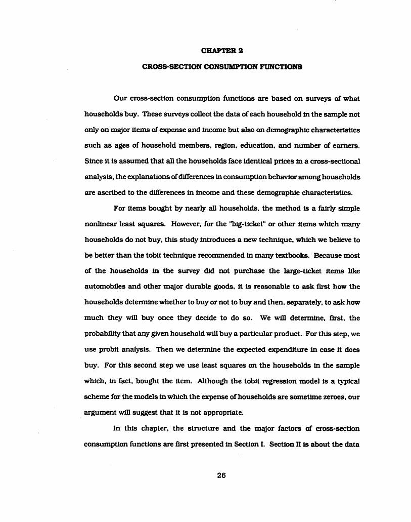
CHAPTER 2

CROSS-SECTION CONSUMPTION FUNCTIONS

O ur cross-section consum ption functions are based on surveys o f w hat

households buy. These surveys co llect the data o f each household in the sam ple no t

on ly on m ajor item s o f expense and incom e b u t also on dem ographic characteristics

such as ages o f household m embers, region, education, and num ber o f earners.

Since it is assumed th a t a ll the households face id en tica l prices in a cross-sectional

ana lysis, the explanations o f differences in consum ption behavior among households

are ascribed to the differences in incom e and these dem ographic characteristics.

For item s bought by nearly a ll households, the m ethod is a fa irly sim ple

non linear least squares. However, fo r the "b ig -ticke t” o r o ther item s w h ich m any

households do no t buy, th is study Introduces a new technique, w h ich we believe to

be be tte r than the to b it technique recommended in m any textbooks. Because m ost

o f the households in the survey d id no t purchase the la rge -ticke t item s like

autom obiles and o ther m ajor durable goods, it is reasonable to ask firs t how the

households determ ine w hether to buy o r no t to buy and then , separately, to ask how

m uch they w ill buy once they decide to do so. We w ill determ ine, firs t, the

p ro b a b ility th a t any given household w ill buy a p a rticu la r product. For th is step, we

use p ro b it analysis. Then we determ ine the expected expenditure in case it does

buy. For th is second step we use least squares on the households in the sam ple

w h ich , in fact, bought the item . A lthough the to b it regression m odel is a typ ica l

scheme fo r the m odels in w h ich the expense o f households are som etim e zeroes, ou r

argum ent w ill suggest th a t it is not appropriate.

In th is chapter, the s tru c tu re and the m ajor facto rs o f cross-section

consum ption functions are firs t presented in Section I. Section n is about the data

26

and the estim ation scheme o f the em pirica l w ork. Section m is the sum m ary o f the

estim ation resu lts o f the least squares m ethod. Section IV conta ins the resu lts

estim ated by the b ig -ticke t-item analysis.

I. The S tructu re o f C ross-Section C onsum ption Functions

A fundam ental no tion in th is study is a non -linea r Engel curve. That is , it

is possible fo r the Engel curve to represent a p a rticu la r good as a lu x u ry fo r some

incom e groups w h ile as a necessity fo r others. A second fundam ental no tion is th a t

o f dem ographic effects. The im pacts o f the dem ographic facto rs on consum er

spending are p a rticu la rly from region o f residence, education, w orking spouse, fam ily

size, and age o f household head. For instance, ou r resu lts w ill show th a t the

households w ith w orking wives spend s ig n ifica n tly m ore than one-earner households

on dom estic servants and laund ry services. A th ird fundam ental no tion is th a t o f the

a d u lt equivalency w eight (AEW). Roughly speaking, the th ird no tion is th a t age and

sex o f household m embers affect th e ir consum ption. A m an aged th irty counts fo r

m ore th a n a g irl aged s ix in the consum ption o f beer. More precise ly, o u r resu lts w ill

show th a t adu lts aged between th irty -o n e and fo rty count fo r m ore th a n 15 tim es as

m uch as do ch ild ren aged under five years in the consum ption o f alcohol.

To express ou r three fundam ental notions in a typ ica l consum ption

fu n ctio n , we can w rite a general form as follow s:

Fam ily consum ption o f product i =

( fj ( Incom e per capita w ith in the fa m ily ) + Dem ographic e ffe c ts )

* ( Fam ily size fo r product i ).

27

A lthough the de ta ils o f each fundam ental no tion w ill be sh o rtly presented, an

overview o f the specific form o f the consum ption fu n ctio n in th is d isse rta tion w ill be

firs t in troduced.

The fu n ctio n a l form used fo r a cross-sectional study m ust be flex ib le enough

to represent the demand fo r lu xu rie s , necessities, and in fe rio r goods. The form

em ployed is 1

Ct * ( bt0 + £ byYj + £ dyD j) ( WtgTig ) (2.1)J J 9

where

Cj is the household consum ption o f good 1;

Yj is the am ount o f per capita household incom e w ith in the J1*1 Income

bracket w h ich w ill be sho rtly described in de ta il;

D j is the j * dem ographic category represented by a zero-one dum m y variab le:

ng is the num ber o f household members in age group g; and

by’s, d jj’s, and w ^ ’s are the coefficients to be estim ated.

In E quation (2.1), household consum ption o f com m odity 1 is explained by

household incom e per capita , dem ographic characte ristics o f the household, and the

weighted household size fo r product i, Xg w lgng. The weighted household size

depends no t on ly on the num ber o f fam ily members b u t also on th e ir ages. Thus,

household consum ption o f good 1 is obtained by m u ltip ly in g expenditure per

household m em ber by the specific size o f household fo r 1. The w eighted size o f a

household d iffe rs by com m odities. In add ition , the w eight fo r each good varies by age

groups.

1This form is borrowed d irectly from Devine (1983), although a different estim ation scheme is applied.

28

A. Incom e vs. C onsum ption E xpenditure

One o f the m ost Im portant facto rs In tra d itio n a l consum ption functions Is

the incom e variab le. Engel curves represent the re la tionsh ip between incom e and

ou tlay o f each p a rticu la r com m odity. Before going in to a discussion o f the functiona l

form , we m ust c la rify the m eaning o f "incom e". Theore tica lly, the level o f household

expenditure depends on the level o f perm anent incom e. In o u r cross-sectional

analysis, to ta l annual expenditure w ill be used to represent perm anent incom e. In

p rin c ip le , "perm anent incom e" re flects past, present, and expected fu tu re incom e, as

w e ll as w ealth. In practice, past Income, expected fu tu re incom e and a general

m easure o f w ealth are no t available. M oreover, even if they were, they are so

corre lated th a t it seems useless to em ploy them separately as explanatory variables.

Besides the a va ila b ility o f data, another d iffic u lty arises when using

"perm anent incom e" as the determ ining variab le in the consum ption functions. In

cross-section, h igher incom e is always associated w ith a h igher saving ra te . The

tim e-series evidence, however, shows th a t, although average Incom es have Increased

su b sta n tia lly , the aggregate saving ra te tends to rem ain constant o r even to decline

s lig h tly over tim e. Hence, if we use any form o f "incom e" as the explanatory variab le,

we w ill underestim ate the increase in the tim e-series aggregate consum ption

expenditures as incom e increases. In the cross-section, we w ill use to ta l expenditure

as the "Incom e" variab le in the consum ption function .

A lthough a va rie ty o f fu n ctio n a l form s o f Engel curves have been

investigated by Brow n and Deaton (1972), each o f the form s they study is good only

fo r a specific group o f com m odities w ith ce rta in characte ristics.2 The Piecewise

2For example, the double-logarithm ic form is not appropriate i f the observed value on the dependent variable is sometimes zero.

29

Linear Engel Curve (PLEC), employed in w hat fo llow s, however, is general and flexib le

enough to represent a ll the groups.

The basic idea o f ou r consum ption fu n c tio n is to represent a fam ily ’s

consum ption as a product o f tw o term s, one depends on the per cap ita incom e w ith in

the fam ily , Y, and the o ther being the fa m ily size fo r th a t product. I t w ill be recalled

th a t the basic equation is :

Fam ily consum ption o f product 1 =

( Jj ( Incom e per cap ita w ith in the fa m ily ) + Dem ographic e ffe c ts )

* ( Fam ily size fo r product i ).

We now tu rn to expla in ing the form o f the f j( ). F igure 2.1 shows an example o f the

form we sh a ll use. a piecewise lin e a r function . We firs t m ark ou t five incom e

brackets, w ith po in ts a t B0. B lt ... , Bs.

30

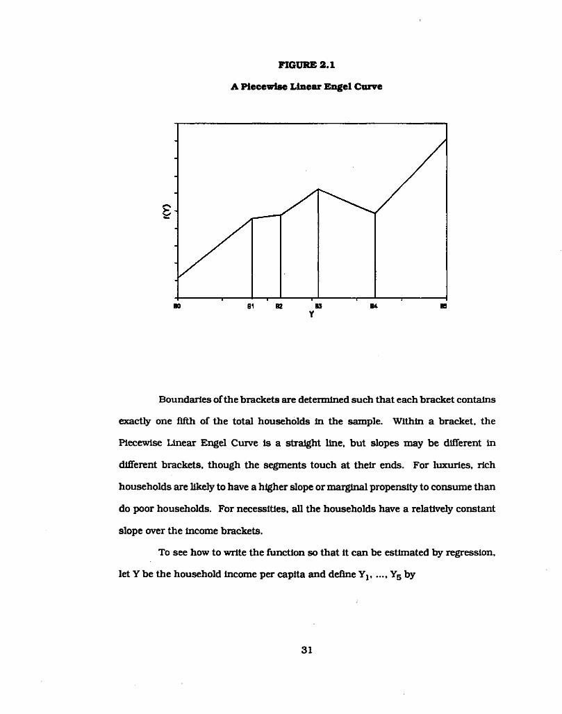
FIGURE 2.1

A Piecewise L inear Engel Curve

Y

Boundaries o f the brackets are determ ined such th a t each bracket contains

exactly one fifth o f the to ta l households in the sam ple. W ith in a bracket, the

Piecewise L inear Engel Curve is a s tra ig h t lin e , b u t slopes m ay be d iffe ren t in

d iffe ren t brackets, though the segments touch a t th e ir ends. For lu xu ries, rich

households are lik e ly to have a h igher slope o r m arg ina l propensity to consume than

do poor households. For necessities, a ll the households have a re la tive ly constant

slope over the incom e brackets.

To see how to w rite the function so th a t it can be estim ated by regression,

le t Y be the household incom e per capita and define Y j...... Y5 by

31

= 0

I f Y £ Bj

I f Bj > Y S B j.!

I f B j.j t Y

Thus, the Piecewise Linear Engel Curve fo r good 1 is described as follow s:

To p u t the same m atte r in w ords, i f the fam ily ’s per cap ita incom e, Y, is

greater than o r equal to the boundary b u t low er than the next boundary Bk+1,

then the fam ily ’s Income in a ll the incom e brackets below B^ is equal to the w id th o f

th a t bracket, w h ile the fam ily ’s Income in the k1*1 bracket is o f the am ount o f the

excess o f Y over Bk, and its incom e in a ll the h igher brackets is zero. A num erica l

exam ple m ay be usefu l here. Suppose the values o f the boundaries are as follow s:

Bq — $0, B j — $2,000, B^ = $4,000, Bg — $6,000, B^ — $8,000, and Bg — in fin ity .

C onsider a household w ith per capita incom e o f $4,500, w h ich fa lls between B2 and

B3. Its Y i’s are: Y j = B j - B0 = $2,000, Y2 = B2 - B j = $2,000, Y3 = Y - B2 = $500,

Y4 = $0. and Y5 = $0.

The coefficient o f Y j, by, is the slope o f Engel curve w ith in bracket J. These

slopes d iffe r no t on ly over d iffe ren t goods b u t also over d iffe ren t incom e levels. Thus,

it is possible to show th a t a p a rticu la r com m odity is a necessity fo r some incom e

groups b u t a lu xu ry fo r others. I f the coefficients o f a ll the incom e brackets are the

same fo r a p a rticu la r com m odity, the Engel curve is linea r.

Recall th a t the boundaries o f incom e. B j's, are determ ined so th a t each

incom e bracket contains exactly one fifth o f the to ta l households in the sam ple. The

re su ltin g boundaries o f ou r data, the 1980-1981 Survey o f Consum er E xpenditures

are as follow s:

M Y ) (2 .2)

32

B0 = $0

B 1=: $3,310

B2 = $4,639

B3 = $6,277

B4 = $8,848

B5 = In fin ity (In the p lo ts, Bs w ill be taken as $12,000 fo r the

estim ated Engel curves)

Thus, the fundam ental equation can now be w ritte n as

Fam ily consum ption o f product 1 =

( fyo + fYj + Dem ographic effects )*( Fam ily size fo r product 1).

B. Household C haracteristics

Given the form we derived in the la s t section, we now tu rn to the discussion

o f dem ographic variables.

a. The E ffect o f Dem ographic Variables

The im pacts o f the dem ographic factors on consum ption expenditures re su lt

especially from region o f residence, education, w orking sta tus o f spouse, fam ily size,

and age o f household head.

33

Region:

The geographic regions are N ortheast, N orth C entra l, South,

and W est. The region o f residence has an apparent in fluence on some

expenditure item s. The households in the W est have a re la tive ly large

num ber o f renters whose u tilitie s are included in ren t. The

expenditures o f these households on e le c tric ity , gas, and w ater thus

are low er w h ile the expenditures on she lte r are h igher th a n those o f

households in other regions. On the o ther hand, the N ortheast has

h is to rica lly accounted fo r a la rger share o f to ta l fue ls and u tilitie s

expenditures than o ther regions m ostly because o f the w eather

conditions. Precise de fin itions o f the regions are given in Appendix

B.

Education:

The education o f household head is classified as e ithe r

college-educated o r not college-educated. Besides the h igh corre la tion

between education and unem ploym ent rates, the households w ith

college educated members spend d iffe re n tly on certa in com m odities

from the fam ilies whose heads are no t college- educated. O ur resu lts

w ill show th a t the expenditures on reading m ate ria ls and ch ild ren 's

education are the m ost s ig n ifica n t item s.

W orking S tatus o f Spouse:

In the 1950’s, less than 20% o f women were wage earners.

Since the la te 1970’s, however, more than 50% o f women have been

w orking or looking fo r w ork in the labor force. The b ig changes in the

34

labor-fo rce-partic ipa tion rate, w hich increases dram atica lly fo r women

b u t declines fo r m en. Influence expenditure pa tte rns especially on the

consum ption o f services. The households w ith w orking w ives spend

s ig n ifica n tly m ore than one-eam er households on dom estic servants

and laund ry services.

Fam ily Size:

Fam ily size is classified in to fo u r groups: one-person; tw o-

person; three o r fo u r persons; and five o r m ore persons. The am ount

o f expenditures m ay not be lin e a rly dependent upon the num ber o f

persons In the households. For exam ple, o ther th ing s being equal,

the use o f indoor lig h tin g w ould provide an inverse re la tionsh ip

between fa m ily size and per capita expenditure on e le c tric ity . Thus,

fam ily size is used to account fo r "econom ies o f scale" In fam ilies

w hich m ay affect per cap ita expenditure w ith in the fam ily .

Age o f Household Head:

The age o f householders is divided in to three categories:

under 35, between 35 and 55, and above 55. As expected, the

householders in the over 55 age group spend a h igher p roportion o f

to ta l expenditures on hea lth care than do o ther age groups. The

m iddle age group, however, spends m ore on tran spo rta tio n and

personal business.

Zero-one dum m y variab les are used to represent the dem ographic factors.

Each household belongs to one and on ly one o f the groups In each category. To

35

avoid co llin e a rity , one o f the groups in each category is le ft ou t. Suppose there are

L dem ographic categories, then the s tru c tu re o f the dum m y variab les w orks as

fo llow s:

D j = 1 if the household is in dem ographic group j

= 0 otherw ise

where j = 1.....L

The le ft-o u t dem ographic group is a rb itra rily picked as 3-4 m em ber

households in the N ortheast region w ith o u t a w orking spouse, and w ith a head aged

group 35-55 w ith o u t college education. The detailed contents o f the dum m y

variab les are then

------- Regional category -------

D j: Region = N orth C entral

D2: Region = South

D3: Region = W est

------- E ducation ca tegory-------

D4: E ducation o f Household Head = College

------- W orking spouse ca te g o ry -------

D5: W orking S tatus o f Spouse = Spouse is Em ployed

------- Fam ily size category -------

D6: Fam ily Size = 1

D7: Fam ily Size = 2

D8: Fam ily Size £ 5

36

------- Age category -------

D9: Age o f Household Head < 35

D 10: Age o f Household Head > 55

In our fu n ctio n a l form (2.1), we assume th a t there are no In te ractions

between the dem ographic variab les, so the to ta l dem ographic effect is add itive:

Dem ographic effects = ]£

Since the dem ographic effects are add itive, they Influence on ly in the In te rcep t o f the

PLEC.

In general, if the in te ractions between these facto rs are no t excluded and we

re s tric t ourselves to the cond ition o f tw o-variable in te ractions, the in te ra c tio n effect

represented by the dum m y variables can be described as3

Dt*D j =1 if there is in te ractio n between

1th and J * dem ographic category

= 0 otherw ise

I t is no t d iin c u lt to construct these in te ractions in the cross-section, though the

num ber o f param eters to be estim ated w ould rise sharp ly (In ou r m odel, the num ber

o f param eters w ith tw o-variab le in te ractions are 4*(2+2+4+3) + 2*(4+2+4+3) +

2*(4+2+4+3) + 3*(4+2+2+4) = 132, since we have to be concerned w ith , fo r exam ple,

3I f a fu ll interaction among these variables is allowed, the product o f up to five dummies should be used as the explanatory variables. In th is case, we may have the demographic in teraction effect o f a household w ith four fam ily members and two earners w hich resides In the Northeast and whose household head Is fifty-five years old and college-educated.

37

no t on ly the effect o f a household w h ich resides in the W est w ith college-educated

household head b u t also the effect o f a tw o-eam er household w hich has a live-year-

o ld ch ild ). The tra n s itio n from the cross-section to the tim e series, however, w ould

be a ve iy com plex task. We w ould need the h is to rica l data fo r a ll the possible

in te ractions among these factors. In fact, they are no t available from our data

sources. The assum ption th a t the dem ographic effect is additive is to make our

tra n s itio n to the tim e-series analysis possible.

Thus, the basic equation incorporated w ith the form o f dem ographic effects

can now be w ritte n as:

Fam ily consum ption o f product 1 =

( *> «> + £ tyY l * dyDj )*( Fam ily size fo r product i ).

b . The E ffect o f Fam ily Com position

How does the age s tructu re o f a household affect its consum ption? To study

th is question, we sh a ll divide the popula tion in to 8 age groups and record the

num ber o f fa m ily members in each group, rig, g= 1,...,8. The unw eighted fam ily size,

n , therefore, is

n = (2.3)9

For each product, we w ish to fin d how m uch one person in each age group

counts re la tive to a person in the reference group, w hich we w ill take to be the 31-40

age group. We w ill ca ll th a t w eight wg fo r group g. Then

38

" i • ' L w ieng (2.4)9

becomes the household size weighted fo r product i. In E quation (2.4), is the

weighted fam ily size fo r good 1 and w ^ is the w eight o f good 1 fo r age group g. The

unw eighted fa m ily size Is a special case o f the weighted sum w ith a ll the w eights

equal to 1.0.

W hile the to ta l expenditure Is divided by the specific size o f the household

fo r each p a rticu la r com m odity to get the per capita household consum ption on th a t

item , the incom e o f the household needs to be divided by an incom e scale to provide

a m ore accurate m easure o f per capita household Income. This incom e scale could

be m easured by the weighted average o f the weights o f d iffe ren t age groups fo r th a t

com m odity w ith w eights approxim ate^ proportiona l to the expenditures on the

com m odities (Prals and H outhakker, 1971). The w eight o f incom e o f good 1 fo r age

group g can be expressed as

where the w eight q j/y is the budget share o f good i. The household size o f Income,

th u s , is

The incom e w eights represented by E quation (2.5) are the weighted AEW’s

fo r d iffe ren t consum ption item s in the economy w ith w eights being shares o f each

corresponding com m odity. This assum ption th u s im plies th a t the overall im pact on

consum ption fo r each age group w ill be disclosed v ia the association o f th e ir specific

in fluences on the d iffe ren t goods. O bviously, the bigger the incom e w eight o f a

ce rta in age group is , the m ore expensive is the m aintenance o f th a t group.

(2.5)

(2.6)9

39

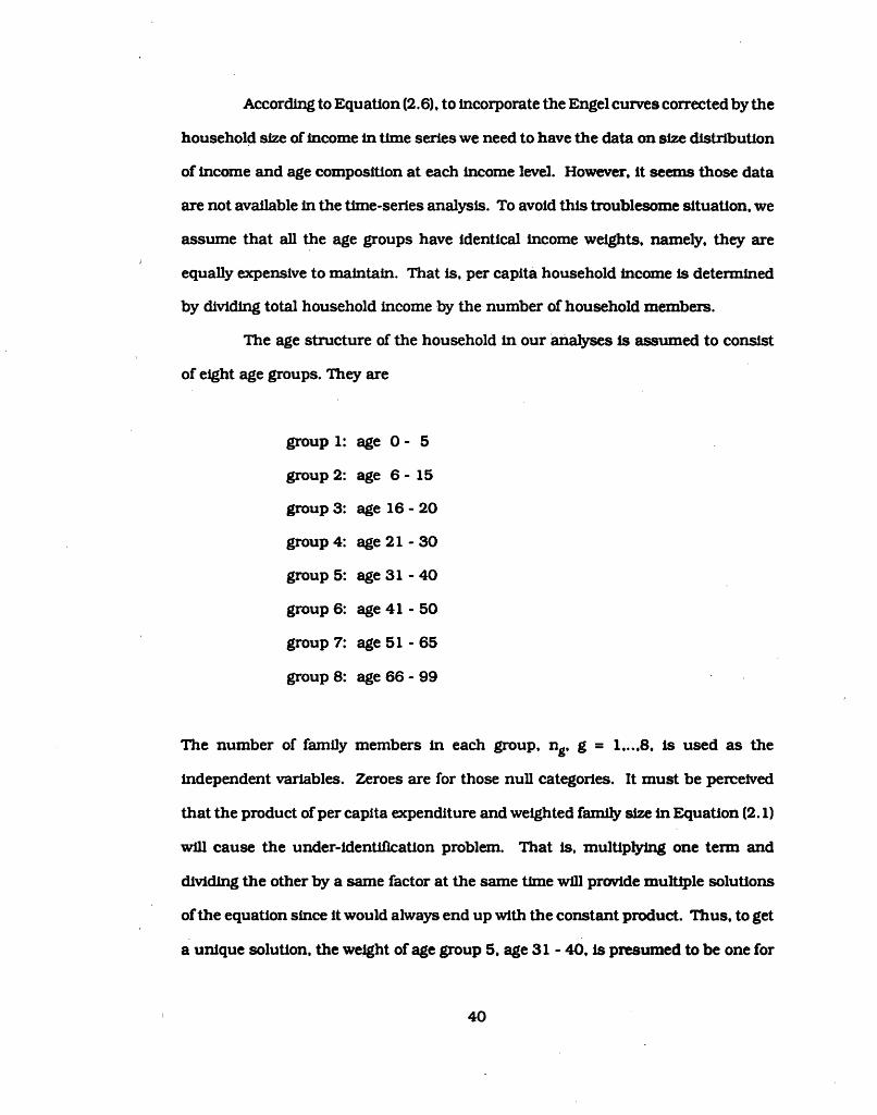
According to E quation (2.6), to incorporate the Engel curves corrected by the

household size o f Incom e In tim e series we need to have the data on size d is trib u tio n

o f incom e and age com position a t each incom e level. However, it seems those data

are no t available in the tim e-series analysis. To avoid th is troublesom e s itu a tio n , we

assume th a t a ll the age groups have iden tica l incom e w eights, nam ely, they are

equally expensive to m a in ta in . That is , per capita household incom e is determ ined

by d iv id ing to ta l household incom e by the num ber o f household m em bers.

The age s tru c tu re o f the household in ou r analyses is assumed to consist

o f e ight age groups. They are

group 1: age 0 - 5

group 2: age 6 - 15

group 3: age 16 - 20

group 4: age 21 - 30

group 5: age 31 - 40

group 6: age 41 - 50

group 7: age 51 - 65

group 8: age 66 - 99

The num ber o f fam ily members in each group, ng, g = 1 ,..,8 , is used as the

independent variables. Zeroes are fo r those n u ll categories. I t m ust be perceived

th a t the product o f per capita expenditure and weighted fam ily size In E quation (2.1)

w ill cause the unde r-iden tifica tio n problem . That is . m u ltip ly in g one te rm and

d iv id in g th e o ther by a same facto r a t the same tim e w ill provide m u ltip le so lu tions

o f the equation since it w ould always end up w ith the constant p roduct. Thus, to get

a unique so lu tion , the w eight o f age group 5. age 31 - 40. is presum ed to be one fo r

40

each o f the categories. I t therefore could be viewed as the reference group o r the

a d u lt equivalent.

Now, we can have a fin a l form o f the equation, w hich conta ins o u r three

fundam ental notions, as follow s:

Fam ily consum ption o f product 1 =

( bto + £ by Yj + M £ u’ igHg )J J 9

C. "B ig -T icke t", Seldom -Bought Item s

For m any la rge -tlcke t Item s like autom obiles and o ther m aj o r durable goods,

zero expenditures are reported by m any I f no t m ost o f the households In the survey.

However, It Is no t reasonable to ju s t use the zeroes fo r expenditures o f those who d id

n o t buy. Instead, we w ill ask: W hat are the p roba b ilitie s o f purchase fo r each

household? W hat is the expected am ount o f expenditures i f it does buy? To answer

these questions, we have to form ulate a m odel w h ich conta ins a d is trib u tio n o f

purchase p ro b a b ility and a consum ption equation w h ich incorporates the

in fo rm a tion o f the p ro b a b ility d is trib u tio n .

a. The Model

O ur approach, in contrast to the to b it approach often used fo r th is problem ,

recognizes th a t the factors determ ining w hether o r n o t a fa m ily buys a p a rticu la r

good m ay be qu ite d iffe ren t from those th a t determ ine the am ount spent, given th a t

41

X

the fam ily buys. For instance, having a new bom baby could be the m ost im portan t

reason fo r a fam ily to decide to buy a new car. However, once the decision to buy is

made, the fam ily 's disposable incom e w ill d icta te the am ount spent.

The approach in th is study is m ore flex ib le than the tra d itio n a l to b it

analysis. A com plete descrip tion o f to b it analysis m odel can be found in Appendix

C. R oughly speaking, to b it analysis form ulates a regression m odel in w hich the

same lin e a r fu n c tio n w hich determ ines how m uch the fam ily spends also determ ines

w hether o r no t it buys by sim ply se tting the purchase equal to zero if the value o f the

lin e a r fu n ctio n is less than 0. H ie ord inary least squares approach w ill cause

estim ation b ias when the dependent variab le is lim ite d in th is way.

O ur c ritic ism o f the to b it m odel is m a in ly on its specification o f the

explanatory variables. In to b it, the variables used to expla in the p ro b a b ility o f

purchase m ust be the same as those th a t in fluence the level o f consum ption.

Indeed, they m ust have the same w eight in both decisions. The above example o f

buying a new car shows th a t th is use o f the same w eights in both decisions is clearly

inappropria te. In contrast, ou r m odel allow s the p o ss ib ility o f using d iffe ren t factors

to answer the two questions: "to buy o r no t to buy?" and "how m uch to spend?"

Furtherm ore, even if the same factors are used, th e ir re la tive Im portance m ay be very

d iffe ren t fo r the tw o questions.

To expla in ou r m ethod, we need to in troduce some nota tion . For each

fam ily, le t the variab le ya be 1 if the fam ily bought product i and otherw ise 0. We

w ill ca ll the row vector o f variab les used to expla in the yes-or-no decision to buy x ^

and denote the w eights o f the variab les in th is decision by the colum n vector By

x ^ we denote the variab les used to explain the am ount spent, y ^ . by those fam ilies

w hich bought. Thus, a general form o f the m odel can be described as

42

«I1 = /n l* l lP t l ) + “ 11

fo r a ll households. The ft l fu n ctio n can be expressed as follow s:

y<i - - jL = / e ^ d t ♦ u „. t 2

(2.7)<j2n

where ua is a dlstuit>ance term , and the in teg ra l is the norm al cum ulative density

fu n ctio n . Then, fo r those who bought,

where f is o u r usua l piecewise lin e a r function , and the u ^ are d isturbance term s.

We w ill denote by yn A the estim ate o f y41 fo r each household and in te rp re t

it as the p ro b a b ility o f purchase by th a t household. B y E quation (2.7), yn A w ill be

ca lcula ted fo r each household.

The expected value o f expenditure fo r a given household, y13, is then the

product o f the p ro b a b ility o f purchase and the am ount spent i f the household buys.

It Is given by the fo llow ing equation:

fo r a ll households. E quation (2.9) makes the expected purchases o f the household

a very non -linea r fu n ctio n o f and x12. A t th is p o in t, we m ust look ahead to the

next chapter to an tic ipa te a problem . In th a t chapter, we sh a ll use the variab le Ct*

w hich Is w hat consum ption per a d u lt equivalent w ould be in period t if it were

determ ined solely from incom e and dem ographic effects, as ascertained from the

cross-section. Thus, fo r a given product.

Ut2 * J ixt2̂ + u(2 (2 .8)

y * Bfn (2.9)

t J J

where the sum on 1 ru n s over a ll households.

43

T h is can be rew ritte n as

c - " E b jE Yu * E djE D0 “ 'E b jY j ♦ £d,D j

where Yj and D j are popula tion to ta ls fo r w hich tim e series can be constructed.

T h is use o f the popula tion to ta ls to construct C* was possible because o f the

lin e a rity o f the consum ption per a d u lt equivalent In the Yy and Dy. U n fortunate ly,

the product o f E quation (2.7) w ith E quation (2.8) y ie lds a fu n c tio n th a t is by no

m eans lin e a r in the determ ining variab les. I f we sim ply stopped w ith the estim ation

o f these two equations, we w ould be unable to com pute the m ovem ent o f to ta l

expenditure o f the popu la tion from available data on the d is trib u tio n o f Income and

the dem ographic variables.

As a way o f dealing w ith th is problem , we estim ated a fu n ctio n o f the norm al

form (Equation (2.1)) by using as the dependent variab le , no t the actua l expenditures

o f the household on "b ig -ticke t" item s, b u t the household's expected expenditure, yi3.

The equation used fo r estim ation can be w ritte n as follow s:

Vi3 “ /U j2) + “ i3 *2101

fo r a ll households, where u i3 is the disturbance term . In th is way, we avoid the

problem o f zero values.

A lthough ou r m odel recognizes th a t the factors affecting the p ro b a b ility o f

purchase m ay no t be the same as those affecting the am ount purchased, we w ill. In

fact. Use the same determ ining variab les fo r both purposes. A ll o f the lim ite d

num ber o f the explanatory variab les in ou r m odel seem possib ly re levant to both

decisions. In term s o f ou r no ta tion , x ^ = x ^ . However, we do no t assume th a t the

jB jj in any way enter the f l x ,2 ) fu n ctio n in equation (2.8).

We w ill, in fact, apply the m ethod in troduced in th is section no t on ly to the

"la rge -ticke t” item s b u t also to the consum ption goods w h ich are re la tive ly

44

inexpensive b u t are no t bought by m any fam ilies. For instance, ou r data shows th a t

about 45% o f the households d id no t buy cigarettes and about 40% o f the fam ilies

reported zero expenditure on alcohol, a lthough these goods are no t "b ig -ticke t" item s.

b. The D ecision to Buy

In th is section we tu rn to the discussion o f the purchase p ro b a b ility

d is trib u tio n functions. The objective o f E quation (2.7) is to determ ine the purchase

p ro b a b ility o f a given product fo r each fam ily . There are tw o com mon approaches to

estim ating the purchasing decision p ro b a b ility fu n c tio n in advance. One is the

p ro b it m odel, and the o ther is the lo g it m odel. In ou r analyses, the p ro b it m odel is

selected as the approach in advance w ith o u t any p a rticu la r reasons. Besides, we w ill

in troduce an approach w hich no t only can be used as an "ex post" test fo r the resu lts

o f the p ro b it m odel b u t also oiTers an a lte rna tive evaluation o f the purchase

p ro b a b ility function . I t is im portan t th a t we investigate w hether the norm al provides

a good approxim ation to the actua l p ro b a b ility d is trib u tio n , because we w ill take its

re su lt seriously as the p ro b a b ility o f purchase in ou r ,rb lg -ticke t" analysis.

The basic idea o f the "ex post" approach is to derive the actua l d is trib u tio n

o f purchase p roba b ility . That is , fo r good 1, we w ill ra n k the households by th e ir

XjjJSj! score, group them in to ventiles, and use the data reported by each fa m ily to

ca lcu la te the num ber o f households who bought in each X j^ j group and then

com pute the corresponding percentage o f those who bought in th a t group. T h is "ex

post" p ro b a b ility fo r households in the ven tile can be com pared w ith the average

p ro b a b ility com puted from the p ro b it fo r those households. There is no a p rio ri

guarantee th a t these two p roba b ilities w ill be iden tica l o r even s im ila r. Should they

prove d iss im ila r, the "ex po rt" p roba b ilities could be used in E quation (2.7). In fact.

45

they tu rned ou t to be qu ite s im ila r and the theore tica l p ro b a b ilitie s were used.

A n a lte rna tive to the p ro b lt m ethod was also trie d . The a lte rna tive m ethod

sim p ly regresses the zero-one variab le , yllt on the determ ining variab le , x ^ , by least

squares. It is given by the fo llow ing equation

yn c xn bn + vn (211)

fo r a ll households, where vt l is the disturbance term .

The usua l objection to th is m ethod is th a t it is hard to in te rp re t the

predicted values; they cannot be p roba b ilities since they m ay fa ll outside the [0,1]

in te rva l. Th is problem o f in te rp re ta tio n is read ily rem edied by the use o f the "ex

post" m ethod. A fte r estim ation, the households are ranked by the value o f

w h ich is estim ated by E quation (2.11). F u rthe r, they are grouped in to tw enty

ven tiles (each ven tlle contains exactly one tw entie th o f the to ta l households). To

com pute the actua l p ro b a b ility o f purchase fo r each ven tile , we sum over the values

o f yn w ith in the ven tlle (since y t l equals one if the household bought, and equals zero

i f the household d id no t buy, the sum o f y ^ 's is the num ber o f households who

bought), and then divide the sum by the num ber o f ven tile ’s households. The

com putation has to be done fo r each ventlle . By doing th is , we get a d is trib u tio n o f

actua l p ro b a b ility over the tw enty ventiles.

The advantage o f th is a lterna tive approach is its low er com puting cost a t the

firs t step. However, the cost o f fun ctio n evaluation a t the second stage is less

expensive fo r p ro b it once the estim ated param eter is obtained. P rob it makes use o f

the established tab le values o f s ta tis tica l p ro b a b ility fo r a ll the equations, w h ile the

"ex post" approach has to construct an in d iv id u a l d is trib u tio n o f p ro b a b ility fo r each

o f the consum ption item s. For the convenience o f fu n ctio n evaluation, we chose to

use the p ro b it analysis in th is study. However, we recognized th a t an "ex post"

testing is necessary.

46

n. Data and Estimation Scheme

A. Data

The data used fo r the cross-sectional analysis is obtained from the

Consum er Expenditure Survey: Interview Survey, 1980-1981. The Consum er

E xpenditure Survey conducted by the Bureau o f Labor S ta tis tics consists o f two

separate com ponents. One is the qua rte rly in terview survey in w hich each o f

households in the sam ple is interview ed once every three m onths over a 12-m onth

period, and the o ther is the d ia ry survey in w hich households are requested to keep

a d ia ry o f expenses fo r tw o consecutive 1-week periods. The in terview survey

accounts fo r approxim ately 95 percent o f to ta l household expenditures and includes

a ll the la rge -tlcke t item s like durable goods.

The 1980-1981 in terview survey is the firs t m ajor survey o f consum er

expenditure since 1972-1973. The ea rlie r survey has been used to analyze cross-

sectional consum ption demand by Devine (1983). Since the new survey is designed

in a ro ta tin g procedure where 20 percent o f the sam ple is dropped and a new group

o f households added each quarte r, on ly the households who pa rtic ipa te in fo u r

consecutive quarters over the period from the firs t qua rte r o f 1980 to the firs t quarter

o f 1982 are selected. There are more than 500 item s o f detailed expenditures in the

o rig in a l tapes o f in terview survey. They are aggregated in to 61 categories shown in

Table 2.1 to m atch the categories o f Personal C onsum ption E xpenditure in the

N ational Incom e and Product Accounts as closely as possible fo r the tim e-series

analysis.

Besides the data on consum ption expenditures, a ll the o ther household

characte ristics are also given in the tape file s. Th is m akes the data on dem ographic

47

and age variab les sim ple to obta in. In order to have as fu ll in fo rm ation as possible

fo r households in the sam ple, those w ith o u t reporting o f region o f residence are

excluded. A few households w ith pecu lia r o r probably erroneously reported am ounts

o f spending on ce rta in consum ption categories were also excluded to avoid b iasing

the estim ates to f it o u tlie r observations o f questionable accuracy. The to ta l

observations available are 4400.

48

TABLE 2.1

C ross-Section C onsum ption Categories

1. Food, o ff prem ise2. Food, on prem ise3. A lcoho lic beverages, o ff prem ise4 . A lcoho lic beverages, on prem ise5. Tobacco products6. Shoes and footw ear7. Women’s and ch ild ren ’s clo th ing8. Men’s and boy’s c lo th ing9. Luggage10. Jew elry and watches11. Laundries, storage, and repa ir o f c lo th ing and shoes12. O ther je w e liy and c lo th ing services13. Personal care14. O wner-occupied housing15. Tenant-occupied housing16. O ther housing17. A dd itions, a lte ra tions, and constructions o f residencies18. H otels and m otels19. F u rn itu re20. K itchen and household appliances21. C hina, glassware, and tableware22. O ther durable house fu rn ish ings23. F loor coverings24. Sem idurable house fu rn ish ings25. E le c tric ity26. N a tu ra l gas27. Fuel o il and coal28. W ood, o ther fu e l, and bottled o r ta n k gas29. W ater and other san ita ry services30. Telephone and telegraph ;31. Dom estic service '32. O ther household operations33. Household insurance34. P rescrip tion drug and sundries35. Physicians36. D enta l and eyes37. O ther m edical services and supplies38. H ospitals and san ita rium s39. H ealth Insurance40. Personal business41. L ife insurance42. New cars43. Used cars44. New and used tru cks o r vans45. T ires and tubes46. A u to accessories and parts47. A u to repa irs

49

TABLE 2.1

C ross-Section C onsum ption C ategories (C ontinued)

48. A u to insurance49. G asoline and o il50. T o lls, parking fees, and reg is tra tion51. Local tran spo rta tio n52. In te rc ity tran spo rta tio n53. Books, m agazines, and newspaper54. Boats, recreationa l vehicles, and pleasure a irc ra ft55. W heel goods, toys, and sport equipm ent56. Radio, TV, recorders, and m usical instrum ents57. Radio, TV, and sound equipm ent repairs and re n ta l58. Fees and adm issions59. O ther recreationa l supplies, equipm ent, and services60. E ducation61. Cash co n trib u tio n

50

B. Estimation Scheme

The rig h t hand side o f E quation (2.1) is the product o f per capita

expenditure and weighted household size. It is no t a lin e a r form , so it cannot be

estim ated by o rd inary least squares d irectly . Therefore, an ite ra tive m ethod m ust be

used. Roughly speaking, an ite ra tive process attem pts to m ake the param eters

converge to the desired so lu tion in however m any steps are necessary. A n in itia l

guess o f the so lu tion w ill be adjusted through each ite ra tio n u n til it is close enough

to th e tru e so lu tion . For estim ation, we sh a ll apply the ite ra tive procedure to the

Taylor series expansion o f E quation (2.1). The lin e a r approxim ation o f Taylor series

fo r E quation (2.1) is as follow s:

AC, - m b l0 ♦ ENYj&by ♦ ENDjAdy * £ X n gAwtgJ J 9

(2.12)

where X and N denote household expenditure per capita and w eighted household size

respectively, and A is the am ount o f changes. I t m ust be perceived th a t X and N are

no t constant. The values o f X and N change th rough every ite ra tio n .

E quation (2.12) is a lin e a r form , th u s it can be estim ated by least squares.

The least squares m ethod Is accom plished by using an Ite ra tive process. The firs t

Ite ra tio n begins w ith the id en tica l equivalent w eights. In o ther w ords, the w eights

o f a ll the age groups are presum ed to be one. Subsequently, the cu rre n t estim ated

param eters are used as the s ta rtin g values o f the fo llow ing ite ra tio n . The ite ra tive

procedure is repeated u n til a ll the estim ated coefficients converge to the sta tiona ry

po in ts o r the am ount o f changes in each o f the coefficients approaches zero.

To illu s tra te the detailed ite ra tive procedure, le t f be a fu n c tio n o f a vector

o f independent variab le x and a vector o f param eter B fo r y so th a t y = f l x ,B ). Thus,

the Taylor series expansion around B ^ , the in itia l guess, is

51

/U B ) = /(x .B (0)) + f ( x ,B ,0,)(B - B (0>) ,2 1 3 >

where f ‘(x ,B (0*) Is the firs t derivatives o f 11 x ,B ) w ith respect to B evaluated a t B(0*.

Thus, we can rew rite the equation as follow s

y « / ( x ,B (0)) + / ‘ (x ,B (0) )*AB(0) (2<14)

where AB(0) = B - B (0)

E quation (2.14) can be estim ated by least squares fo r A B ^. Since the value

o f the param eter fo r the next ite ra tio n , Bl l \ equals B ^ + AB(0), f and f * can then be

evaluated a t B fl) in Equation (2.14) to obta in the least squares estim ate fo r AB(1).

Thus, fo r the i+ l^ ite ra tio n , B*1+1* = B® + AB^. That is , the cu rre n t estim ate o f the

changes in param eter B, AB®, is used to provide the value o f B in the next ite ra tio n ,

B&+1\ and then to evaluate the fu n ctio n f and f ‘ a t B®+1*. The process is repeated

u n til the difference between the estim ate in two consecutive ite ra tion s. AB^, becomes

less th a n .01. Th is procedure has to be done fo r each o f the 61 equations. Each

equation has 24 independent variab les and 4400 observations. Therefore, the

ite ra tive procedure is repeated u n til each o f the 24 param eters in a given equation

is converged. By any standard, it is ve iy com puter Intensive.

To estim ate the "b ig -ticke t" item s represented by E quation (2.10), we need

the household's expected expenditure. Thus, we have to firs t estim ate the p roba b ility

o f purchasing fo r each household and the am ount spent by those fam ilies w hich

bought. E quation (2.7) determ ines the household’s p ro b a b ility o f purchasing and

E quation (2.8) provides the am ount o f expenditure fo r those households w hich

bought. To estim ate (2.7), we need to obta in the param eters w h ich m axim ize the

objective function . The objective fu n ctio n o f th is p ro b it m odel is a non linear form .

52

Thus, an ite ra tive process has to be used. We u tiliz e the Newton-Raphson4 m ethod

to estim ate the equations. In the estim ation process, the cum ulative density function

o f standard norm al d is trib u tio n Is repeatedly evaluated a t d iffe ren t po in ts in each

ite ra tio n u n til the convergence o f the fu n ctio n param eters Is achieved.

The estim ation scheme fo r E quation (2.8) Is the same as th a t fo r Equation

(2.1). We firs t approxim ate the equation by the Taylor series expansion, and then

use the ite ra tive procedure to y ie ld the sta tionary estim ates. The on ly difference in

estim ating these tw o equations is the dependent variables. The dependent variab le

in E quation (2.8) Is the am ount spent by those fam ilies w hich bought. We now can

create the dependent variab le, the household’s expected expenditure, fo r Equation

(2.10) by m u ltip ly in g the p ro b a b ility o f purchase by the am ount o f expense I f one w ill

buy. The estim ation procedure fo r (2.10) is also the same as th a t fo r (2.1).

m . E stim a tion R esults o f Least Squares M ethod

O ur regression resu lts show th a t a ll the equations converge except Equation

(17) o f A dd itions, a lte ra tions, and constructions o f residencies. The deta ils o f the

estim ation resu lts are shown In Table 2.2. The figures In the parentheses are the t

s ta tis tics . For a d u lt equivalency w eights, the t values are calculated w ith respect to

the deviations from 1.0, the reference adu lt equivalent.

A. O bservations on Engel Curves

The p lo ts o f the estim ated Engel curve are presented In F igure 2.2. The

curves are draw n fo r the reference household, w hich Is composed o f three o r fo u r

4See Appendix C for the estim ation scheme o f the Newton-Raphson iterative procedure.

53

m em bers and resides in the N orth East region, w ith a non-college educated

householder aged between 35 and 55 and w ith a non-w orking spouse. In F igure 2.2,

the consum ption expenditure per a d u lt equivalent on the ve rtica l axis is p lo tted

against per capita household incom e (w hich Is per cap ita to ta l household

expenditures by o u r de fin ition ) on the horizon ta l axis. In general, there are no great

surprises though it also is dea r from the p ictu res th a t m ost o f the consum ption

item s have ra th e r d is tin c tive Engel curves. We sum m arize the resu lts by the groups

o f equations w ith s im ila r characteristics.

a. Food. A lcohol, and Tobacco

O ff-prem ise consum ption o f both Food (1) and A lcoho lic beverages (3) show

a de fin ite necessity pa tte rn o f consum ption. I t takes a sm aller share o f the budget

as Income gets h igher. On the o ther hand, O n-prem ise consum ption o f Food (2) and

A lcohol (4) are lu xu rie s p a rticu la rly fo r the h igh incom e groups. (The Engel curves

are steeper In the upper levels o f Income). Besides the negative slope o f the th ird

incom e bracket, the consum ption o f Tobacco products (5) show the p a tte rn o f a

necessity.

b . Apparel. Luggage, and Jew elry and W atches

The equations on Apparel, Shoes and footw ear (6), W omen’s and ch ild ren ’s

c lo th ing (7), and Men’s and boy’s c lo th ing (8), show a re la tive ly constant slope o f

Engel curves throughout a ll the incom e brackets. Luggage (9) and Jew elry and

watches (10) are lu xu ries except fo r the th ird and the fo u rth bracket respectively.

The services on these item s. O ther Jewelry and c lo th ing services (12), and Laundries,

storage, and repa ir o f c lo th ing and shoes (11) are m ore lik e lu xu rie s fo r low w hile

necessities fo r h igh Incom e fam ilies. Personal Care (13), as excepted, has a necessity

54

patte rn .

c. S helter

O ur resu lts show th a t h igh incom e households have re la tive ly large shares

o f budget on O wner-occupied housing (14), w h ile low incom e fam ilies spend m ore on

Tenant-occupied housing (15). M oreover, the U-shaped Engel curve fo r E quation (15)

ind ica tes th a t Tenant-occupied housing is an in fe rio r good fo r the low incom e groups.

The slope is negative w ith in the low incom e bracket because low incom e fam ilies w ill

move to the owner-occupied housing as th e ir incom e increases. However, the curve

tu rn s upw ard a t upper levels o f incom e because high incom e fam ilies are lik e ly to live

in the expensive apartm ents. The Engel curves fo r O ther housing (16) show the

slopes firs t clim b ing and then descending. The expenditure on H otels and m otels

(18) is ra th e r a lu xu ry .

d. House Furn ish ings and Equipm ent

In general, a ll the equations o f house fu rn ish ings and equipm ent (19) - (24)

reveal a lu xu ry na ture except fo r K itchen and household appliances (20). A d is tin c t

p a tte rn o f the Engel curves is shown fo r Sem idurable house fu rn ish ings (24). The

second and the fo u rth incom e bracket o f (24) have a re la tive ly h igh MPC. This

phenom enon can be explained by the increase in the q u a n tity o f spending fo r the

second bracket w h ile the progress o f the q u a lity o f consum ption fo r the fo u rth .

e. U tilitie s

A lm ost a ll the u tility expenditures. E quation (25) - (30), have a unique

p a tte rn o f Incom e-expenditure re la tionsh ip . They are a ll necessities undoubtedly.

The on ly exception is W ood, other fue l, and bo ttled o r ta n k gas (28). The possible

55

reason is . s tric tly speaking, they should no t be classified in to u tilitie s . Telephone

and telegraph (30) has a sharpest slope in the firs t incom e bracket follow ed by the

fifth . The in tu itiv e in te rp re ta tio n is th a t the basic fees account fo r the highest MPC

in the lowest bracket. On the o ther hand, the expenses on the long distance phone

ca lls are a ttrib u te d to the am ount o f phone b ill fo r the richest fam ilies.

f. Household O perations

Dom estic services (31) and O ther household operations (32) are m ore lik e ly

to be a lu xu ry . The re su lt shows th a t the MPC o f the highest incom e group fo r these

tw o equations is about ten tim es o f th a t o f the low est bracket. On the o ther hand.

Household insurance (33) is de fin ite ly a necessity.

g. H ealth Care

B asica lly, we expect a necessity pa tte rn o f Engel curves fo r hea lth care.

E quation (34) - (39), since the expenditures o f them are heavily dependent upon the

hea lth cond itions no m atte r one is ric h o r poor. Indeed, the estim ation re su lt shows

th a t except H ospitals and san ita rium s (38), a ll the o ther equations disclose a

necessity type o f Engel curves.

h . Personal Business and L ife Insurance

Personal business (40) and L ife insurance (41) have re la tive ly constant

slopes o f Engel curves th roughout the incom e brackets.

1. T ransporta tion

Except fo r New cars (42) and New and used tru cks o r vans (44), a ll the o ther

expenditures on autom obiles have a s im ila r Engel curve. That Is, they do no t take

56

up a la rger share o f budget fo r b e tte r-o ff households. New cars (42) Is undoubtedly

a lu xu ry . Local tran spo rta tio n (51) has ve iy sm all values on MPC’s. In te rc ity

tran spo rta tio n (52), however, has lu x u ry good characteristics.

j. Reading and E nterta inm ent

Books, magazines, and newspaper (53) does no t show a iry p a rtic u la r trend

o f MPC’s. It is highest in the second and the fo u rth incom e bracket and about the

same in others. The re la tive ly expensive enterta inm ent categories like Boats. RV,

and pleasure a irc ra ft (54) and Fees and adm issions (58) have la rge r shares o f incom e

fo r h igher incom e brackets than th a t o f low er ones. Thus, they are lu xu rie s . O ther

enterta inm ent item s have re la tive ly constant slopes o f Engel curves.

k . E ducation and Cash C on tribu tion

It is su rp ris ing th a t E ducation (60) is alm ost unre lated to incom e. The

slopes o f five incom e brackets altogether are s ta tis tic a lly in s ig n ifica n t. The tendency

to Cash co n trib u tio n (61) is obviously h igher fo r rich fam ilies than th a t o f the poor.

B. Im pact o f Dem ographic Variables

The effects o f dem ographic variab les on each in d iv id u a l consum ption item

are presented in Table 2.3. They are ind ica ted by (+) o r (-) if the dem ographic factors

have a s ig n ifica n t positive o r negative im pact on the m agnitude o f a given

consum ption category a t .10 level o f significance.

57

a. Region

40 ou t o f 60 equations are s ig n ifica n t a t .10 level fo r a t least one region

category. I t is shown th a t the N ortheast has a highest share in O wner-occupied

housing (14) w h ile the W est in Tenant-occupied housing (15). On the o ther hand,

households in the N ortheast and in the W est, respectively, have a h ighest share in

Fuel o il and coal (27) and a lowest share in E le c tric ity (25). A nother fin d in g is th a t

the South region has highest share in E le c tric ity (25). I t m ay be a ttrib u te d to the

e lectric heating system s w hich are m ostly b u ilt in the South.

b . E ducation o f Household Head

40 ou t o f 60 equations have a s ig n ifica n t im pact fo r education. The college-

educated householders typ ica lly tend to consume less on A lcohol, (3) and (4), and

Tobacco (5) w h ile spend m ore on Readings (53), and Fees and adm issions (58) than

otherw ise.

c. W orking S tatus o f Spouse

For 16 ou t o f 60 equations, w orking sta tus o f spouse con tribu tes to various

consum ption patterns. The fam ilies w ith two earners spend m ore on Dom estic

services (31) than do those w ith a non-w orking spouse. It ind ica tes th a t the

re s tric tio n o f tim e-budget leads to a d im in ish ing share o f housew ork w ith wom en's

increasing p a rtic ip a tio n in the labor force.

d. Fam ily Size

There is highest p roportion o f the equations w ith s ig n ifica n t in fluence o f

fa m ily size. 42 out o f 60 equations are s ig n ifica n t a t .10 level. Fam ily size is

negatively corre lated w ith the am ount o f per cap ita expenditure on E le c tric ity (25)

58

and N a tu ra l gas (26) because these services can be shared by fam ily m em bers. This

is know n as the economies o f scales in consum ption.

e. Age o f Household Head

A t least one o f the two age variab les fo r household head is s ig n ifica n t in 22

ou t o f 60 equations. It is expected th a t householders in the over-55 age group spend

a h igher p ropo rtion o f th e ir income on housing and hea lth care th a n do the o ther two

groups. The resu lts , however, show th a t the consum ption o f these tw o item s does

no t s ig n ifica n tly d iffe r among the three life cycle stages. T h is is probably because o f

the tren d o f Increasing life expectancy. A threshold o f s ix ty-five years o ld fo r the

th ird life cycle stage m ay re flect the anticipated patterns.

C. O bservations on A d u lt E quivalency W eights

The ba r ch a rt representation o f the adu lt equivalency w eights is qu ite

h e lp fu l here. They are graphed equation by equation in F igure 2.3. I t is clear from

the p ictu res th a t age m atters fo r m ost o f the consum ption item s. Furtherm ore, it is

hard to fin d a p a rticu la r pa tte rn o f the d is trib u tio n o f a d u lt equivalency w eights

between any tw o o r among m ore than two o f the 60 equations. A general sum m ary

made by age groups is as follow s:

a. Age group 1: 0 -5

C hildren under five years old have the highest w eights on Dom estic services,

w h ich obviously is the expense o f baby-s itting and o ther home care fo r ch ild ren ,

F u rn itu re , and Floor coverings. In add ition , they con tribu te alm ost no th ing to the

consum ption o f alcohol. A nother in te resting fin d in g fo r th is group is th a t th e ir

59

w eight fo r T rucks o r vans is equal to alm ost three tim es o f the a d u lt equivalent.

b . Age group 2: 6-15

T h is age group has the highest w eights on Shoes and footwear. C loth ing,

and Luggage. I t is obvious th a t the ch ild ren in th is age group are grow ing faste r

th a n any o ther groups. Thus, the am ount o f the expenditures on apparel are

typ ica lly h igh.

c. Age group 3: 16-20

As expected, th is age group has re la tive ly h igh equivalency w eights on A uto

insurance and Education. B u t there is no in tu itiv e explanation fo r one outcom e.

T ha t Is, th is group is o f eight tim es o f the a d u lt equivalent on the H ospitals and

san ita rium s. However, the p re lim ina ry exam ination o f the data d id no t show any

pecu lia r am ount o f the expenses on hosp ita ls among the households.

d. Age group 4: 21-30

The w eights o f the On-prem ise consum ption both o f food and o f alcohol are

highest In th is group. Th is group also has the highest w eight on autom obiles, both

New cars and Used cars.

e. Age group 6: 41-50

G enerally speaking, th is group possesses alm ost the same weights fo r m ost

o f the consum ption item s as those o f the reference group, age 30 - 41. That is , the

estim ated w eights fo r th is group are no t s ig n ifica n tly deviated from 1.0, the adu lt

equivalent. The b ig differences in consum ption between these tw o age groups are the

d im in ish ing consum ption o f alcohol and the fewer expenditures on fu rn itu re fo r

60

in d iv idua ls aged 41-50.

f. Age group 7: 51-65

The a d u lt equivalency w eights fo r th is group are very close to those o f age

group 8, 6 6 -9 9 , fo r m any equations. B u t the expenditures on m edical services and

supplies are m uch low er. Th is is consistent w ith our find ings on the effect o f age o f

household head.

g. Age group 8: 66-99

It is shown th a t persons in the over 66 age group have the highest w eights

in housing, personal care, m edical expenses, and readings. B u t they account fo r the

consum ption o f alcohol and tobacco only less than h a lf o f the a d u lt equivalent.

IV . E stim a tion R esults o f the "B ig -T icke t" Item s

The m odel fo r the ,'b ig -ticke t" item s is designed p a rticu la rly fo r the

consum ption item s w hich are expensive o r re la tive ly inexpensive b u t are no t bought

by m any fam ilies. I t is expected th a t fo r the item s w hich are bought by m any

households, the estim ated coefficients from th is approach and the least squares

m ethod w ill no t have b ig difference. We ran th is regression fo r a ll the equations and

the resu lts confirm ou r p rio r an tic ipa tion . Table 2.4 shows the coefficients estim ated

by these tw o d iffe ren t m ethods. The firs t colum n is the b ig -ticke t-ltem analysis,

denoted as "p rob it". The second colum n Is the least squares m ethod using a ll

observations. We also include the resu lts o f the least squares m ethod using nonzero

observations in the th ird colum n o f Table 2.4. The num ber o f the nonzero

observations fo r each equation is shown a t the bottom o f the table.

61

The t-s ta tis tic s o f the param eters and R2 fo r m ost equations estim ated by

the "p rob lt" m ethod are extrem ely h igh. T ills Is because th a t we used the expected

values o f consum ption expenditures as the dependent variab le. This dependent

variab le was created by using the estim ation resu lts o f the am ount spent by

households w hich bought, w h ich are shown in the th ird colum n In Table 2.4, and the

p ro b a b ility o f purchase fo r a ll households. Thus, the equations, in th is case, are

fitte d qu ite w e ll by the explanatory variables. Since alm ost a ll the t-s ta tis tic s are fa r

above the values o f the 1% sig n ifica n t level, we sh a ll no t lis t these figures in the

tables.

The more expensive item s like New cars (42), New and used tru cks o r vans

(44), and Boats. RV, and pleasure a irc ra ft (54) have qu ite d iffe ren t resu lts from the

tw o d iffe ren t approaches. For incom e effect, in th is case the m arg ina l propensity to

consume o r the coefficients o f the Income variables, the "p ro b it" m ethod has less

Income im pact than the least squares m ethod does. That is , the Increase In the

expected am ount spent out o f an add itiona l d o lla r in household incom e estim ated by

the "p rob it" m ethod is less than the m arginal increase in spending estim ated by the

least squares m ethod. For dem ographic effect, each estim ated coefficient has the

same sign from these two approaches despite the differences in m agnitude.

For m ost o ther equations estim ated by the "p rob it" m ethod, the effects o f

incom e and dem ographic factors on consum ption are qu ite s im ila r w ith th a t o f the

least squares m ethod. Thus, we sha ll no t repeat the sum m ary o f the estim ation

resu lts fo r each equation and the charts fo r Engel curve and a d u lt equivalency

w eights.

62

TABLE 2.2

E stim ated C oefficients by Least Squares

Variable L is t

VAR 1 - constant

VAR 2 - incom e between $0 and $3,310

VAR 3 - Income between $3,310 and $4,639

VAR 4 - incom e between $4,639 and $6,277

VAR 5 - incom e between $6,277 and $8,848

VAR 6 - incom e over $8,848

VAR 7 - household resides in the N orth C entral

VAR 8 - household resides in the South

VAR 9 - household resides in the W est

VAR 10 - household head is college educated

VAR 11 spouse is employed

VAR 12 - household has one member

VAR 13 - household has two members

VAR 14 - household has live and m ore members

VAR 15 - age o f household head is less than 35

VAR 16 - age o f household head is greater than 55

63

EQUATION 1 FOOD, OFF PREMISE RSQ - 0 .6 1 6 MEAN - 2 9 4 2 .1 7

VAR 1 VAR 2 VAR 3 VAR 4 VAR 5 VAR 6 VAR 7 VAR 8 VAR 9 VAR103 6 3 .2 7 4 “ 7 7 2 7 5 0 .0 9 1 7 7 7 E 7 751077 0 .0 4 0 -■109.396 —8 1 .6 6 7 ■28.916 -8 1 .8 6 9(1 0 .4 5 ) (1 8 .1 4 ) (5 .6 3 ) (4 .3 1 ) (7 .1 5 ) (1 0 .7 3 ) (7 .3 9 ) (5 .4 9 ) (1 .7 7 ) (6 .7 9 )

VAR11 VAR12 VAR13 VAR14 VAR15 VAR16-8 7 7 T 9 ? 2773 IS -■13.969 - 1 6 .4 1 9 5 1 .8 4 9 3 4 .4 5 6

(6 .4 1 ) (0 .6 3 ) (0 .6 5 ) (1 .2 1 ) (2 .8 9 ) (1 .7 2 )0 - 5 6 -1 5 1 6 -2 0 2 1 -3 0 3 1 -4 0 4 1 -5 0 5 1 -6 5 6 6 -9 9

7 7 7 T T b . 934 77 5T S b . 862 l . o o f l 1 .1 3 5 T.OST 7 7 3 5 T(5 .7 5 ) (1 .4 3 ) (2 .0 1 ) (5 .0 1 ) (0 .0 0 ) (4 .4 9 ) (2 .3 8 ) (1 .0 9 )

EQUATION 2 FOOD, ON PREMISE RSQ - 0 .4 4 5 MEAN - 8 1 1 .9 1

VAR 1 VAR 2 VAR 3 VAR 4 VAR 5 VAR 6 VAR 7 VAR 8 VAR 9 VAR10-4 T T T 9 7 ■ O.'OSl b .06 3 0 . 092 6 .0 4 7 0 .0 9 4 7 7 5 5 5 ’ -1 8 .9 3 7 -0 .8 1 2 477337

(1 .6 3 ) (6 .3 5 ) (4 .7 2 ) (7 .1 9 ) (5 .4 0 ) (1 9 .1 3 ) (0 .8 2 ) (1 .6 0 ) (0 .0 6 ) (4 .9 8 )VAR 11 VAR 12 VAR13 VAR14 VAR15 VAR16

-lTTETTO 15 .t) 8 5 1 0 .8 7 8 1^1955 7 7 9 7 7 -T70TJ7(1 .2 6 ) (0 .4 6 ) (0 .6 5 ) (1 .5 9 ) (0 .2 3 ) (0 .2 2 )

0 - 5 6 -1 5 1 6 -2 0 2 1 -3 0 3 1 -4 0 4 1 -5 0 5 1 -6 5 6 6 -9 90 .2 7 0 7 7 5 7 5 1 .4 2 6 T T ffTT 1 .bo o T 7C 77 7 7 5 5 ff 7 7 5 E 7

(7 .0 2 ) (5 .6 6 ) (4 .6 5 ) (0 .2 8 ) (0 .0 0 ) (0 .1 3 ) (8 .9 1 ) (3 .6 4 )

EQUATION 3 ALCOHOL, OFF PREMISE RSQ - 0 .1 4 4 MEAN - 1 5 2 .8 5

VAR 1 VAR 2 VAR 3 VAR 4 VAR 5 VAR 6 VAR 7 VAR 8 VAR 9 VAR10-2 .3 8 0 ■ 0 .0 2 2 0 .0 1 0 6 .0 1 3 b .0 1 3 6 .0 1 2 -1 2 .6 2 1 -773TTT 2 .3 4 8 -8 .6 1 8(0 .1 8 ) (4 .7 8 ) (1 .7 6 ) (2 .4 1 ) (3 .7 4 ) (9 .3 4 ) (2 .4 5 ) (1 .4 3 ) (0 .4 1 ) (2 .0 8 )VAR11 VAR12 VAR13 VAR14 VAR15 VAR16

-7 7 7 5 7 3775S7 3 l .001 2 .6 0 3 T .8 4 9 •-1 7 7 T 5 7(1 .6 2 ) (2 .8 7 ) (4 .6 4 ) (0 .5 3 ) (1 .3 3 ) (2 .3 7 )

0 - 5 6 -1 5 1 6 -2 0 2 1 -3 0 3 1 -4 0 4 1 -5 0 5 1 -6 5 6 6 -9 9b . 6 .2 0 2 0 .4 6 1 7 7 7 5 7 T77OT 0 . 80^ b .6 7 8 0 .4 5 9

( 8 . 2 2 ) (9 .8 3 ) (6 .3 1 ) (3 .5 3 ) (0 .0 0 ) (3 .1 2 ) (6 .0 2 ) (9 .8 9 )

EQUATION 4 ALCOHOL, ON PREMISE RSQ - 0 .1 9 0 MEAN - 1 0 5 .5 3

VAR 1 VAR 2 VAR 3 VAR 4 VAR 5 VAR 6 VAR 7 VAR 8 VAR 9 VAR10-3 TB 3 4 “ O i l 6 .0 1 3 O .b ld 6 .0 0 7 0 .0 2 3 -7 7 7 3 7 -2 0 .0 8 5 - 0 . 2 os -1 .9 9 1(0 .3 5 ) (2 .9 8 ) (2 .4 9 ) (2 .0 8 ) (2 .0 7 ) (1 2 .8 4 ) (1 .0 8 ) (4 .0 8 ) (0 .0 4 ) (2 .1 4 )VAR11 VAR12 VAR13 VAR14 VAR15 VAR16

-2 .1 8 4 1 7 7 .5 3 4 i £ .§ 6 6 4 .4 ^ 2 T T T O - 4 .2 7 6(0 .5 1 ) (8 .4 2 ) (2 .6 3 ) (1 .0 7 ) (0 .0 4 ) (0 .7 1 )

0 - 5 6 -1 5 1 6 -2 0 21 -3 0 3 1 -4 0 41 -50 5 1 -6 5 6 6 -9 9—b .1 8 9 7 7 T 5 T 0 .7 8 5 T 7T 7S ttctto 775S S f l . i i a 0 .2 4 4(6 .5 1 ) (4 .3 7 ) (1 .9 7 ) (1 .7 8 ) (0 .0 0 ) (8 .1 0 ) (1 7 .7 4 ) (1 6 .8 4 )

EQUATION 5 TOBACCO PRODUCTS RSQ - 0 .1 2 1 MEAN = 1 7 6 .1 6

VAR 1 VAR 2 VAR 3 VAR 4 VAR 5 VAR 6 VAR 7 VAR 8 VAR 9 VAR103 9 .b20 I T . 021 0 .0 0 & -0 .0 0 7 0 .0 6 4 b . 002 -77777? -1 7 7 2 7 7 -■19.143 -3 7 7 7 7 T(3 .8 6 ) (5 .9 5 ) (1 .9 3 ) (1 .5 7 ) (1 .2 4 ) (1 .7 0 ) (1 .9 0 ) (3 .1 8 ) (4 .0 9 ) (8 .7 0 )VAR11 VAR12 VAR13 VAR14 VAR15 VAR16

-2 .1 4 1 3 9 .1 8 3 2 3 .5 6 0 -T 77T C 2 .6 9 8 - 7 .4 3 9(0 .7 5 ) (3 .6 0 ) (4 .2 1 ) (1 .8 4 ) (0 .4 3 ) (1 .4 4 )

0 - 5 6 -1 5 16 -2 0 2 1 -3 0 3 1 -4 0 41 -50 5 1 -6 5 6 6 -9 90 .4 2 1 6 .3 9 5 0 .6 9 9 7 7 7 S 7 T7TTW 1 .0 1 0 b .9 2 6 6 .4 1 6

(4 .9 1 ) (6 .7 5 ) (3 .0 0 ) (3 .1 6 ) (0 .0 0 ) (0 .1 2 ) (0 .9 0 ) (1 0 .1 9 )

EQUATION 6 SHOES & FOOTWEAR RSQ - 0 .3 5 4 MEAN - 1 1 0 .2 5

VAR 1 VAR 2 VAR 3 VAR 4 VAR 5 VAR 6 VAR 7 VAR 8 VAR 9 VAR10T .2 1 9 " o : 009 0 .0 0 4 •070TT? 0 .0 0 7 b .o o i —b .98 3 -7 7 9 7 5 ’ -770T1> T 7 3 T 7

(0 .4 3 ) (8 .0 4 ) (2 .9 7 ) (5 .9 9 ) (6 .1 9 ) (1 0 .5 7 ) (0 .7 2 ) (0 .7 1 ) (1 .9 7 ) (4 .0 2 )VAR11 VAR12 VAR13 VAR14 VAR15 VAR16

-0 .0 7 2 1 3 .1 8 8 6 .6 2 0 0 .9 4 7 -1 .7 1 4(0 .0 6 ) (2 .5 8 ) (2 .6 8 ) (0 .7 9 ) (1 .2 8 ) (1 .6 6 )

0 - 5 6 -1 5 1 6 -20 21 -3 0 3 1 -4 0 41 -5 0 5 1 -6 5 6 6 -9 90 .6 7 0 T 7 T 5 5 ■ r a r e 0 .8 6 1 1 .0 0 0 778T C T7T& T5775S

(2 .7 6 ) (3 .8 7 ) (0 .5 8 ) (2 .5 3 ) (0 .0 0 ) (2 .8 4 ) (5 .5 2 ) (9 .9 9 )

EQUATION 7 WOMEN'S fi CHILDREN'S CLOTHING RSQ - 0 .3 7 3 MEAN - 4 0 2 .4 0

VAR 1 VAR 2 VAR 3 VAR 4 VAR 5 VAR 6 VAR 7 VAR 8 VAR 9 VAR10-9 .5 7 1 '0 . 0 2 5 S . 028 0 .0 2 1 ■071377 T5.’037 T T 7 7 7 - 2 .9 3 4 -■11.085 1 0 .2 9 6(0 .9 0 ) (6 .3 0 ) (4 .8 6 ) (3 .7 3 ) (6 .3 9 ) (1 3 .5 4 ) (0 .8 8 ) (0 .5 9 ) (1 .9 8 ) (2 .5 2 )VAR11 VAR12 VAR13 VAR14 VAR15 VAR16

- r n r r c •- 1 6 .§9 2 9 .0 6 4 7 7 5 7 7 -1 4 .6 7 9(1 .3 6 ) (1 .0 9 ) (0 .4 7 ) (2 .0 4 ) (0 .1 2 ) (2 .4 6 )

0 - 5 6 -1 5 1 6 -2 0 2 1 -3 0 3 1 -4 0 41 -5 0 5 1 -6 5 6 6 -9 9T 7 5 T 7 T 7 3 7 7 rrm 0 .8 4 1 l . b f lb 1 .0 3 1 T 7 5S 7 0 .8 2 7(0 .0 7 ) (2 .4 6 ) (6 .2 1 ) (2 .2 1 ) (0 .0 0 ) (0 .3 9 ) (0 .0 4 ) (2 .1 5 )

64

EQUATION 8 MEN'S & BOY'S CLOTHING RSQ - 0 .3 5 9 MEAN - 2 2 8 .6 1

VAR 1 VAR 2 VAR 3 VAR 4 VAR 5 VAR 6 VAR 7 VAR 8 VAR 9 VAR102. bib " o : o i 5 6 .o 2 2 6 .0 1 4 b.622 0 .0 1 9 -7 7 7 T 7 -T 7 7 7 T -■111677 177757

<0 .3 2 ) (5 .4 6 ) (5 .3 6 ) (3 .5 3 ) (7 .3 2 ) (1 2 .4 8 ) (0 .7 3 ) (1 .7 1 ) (3 .3 1 ) (5 .9 1 )VAR 11 VAR 12 VAR13 VAR14 VAR15 VAR16

.3 5 2 ■43.612 * iT ^ E T 7 .0 2 3 - j .2 4 9 —67537(1 .6 7 ) (3 .4 5 ) (1 .9 1 ) (2 .1 3 ) (0 .8 9 ) (1 .5 1 )

0 - 5 6 -1 5 1 6 -2 0 2 1 -3 0 3 1 -4 0 4 1 -5 0 5 1 -6 5 66^990 .4 3 2 1.1364 13757? 1 .6 6 0 0 .9 6 5 0 .8 1 8 6 .5 5 1

(4 .3 2 ) (2 .2 4 ) (0 .4 0 ) (0 .5 8 ) (0 .0 0 ) (0 .5 0 ) (2 .9 5 ) (6 .8 2 )

EQUATION 9 LUGGAGE RSQ - 0 .0 9 7 MEAN 6 .8 9

VAR 1 VAR 2 VAR 3 VAR 4 VAR 5 VAR 6 VAR 7 VAR 8 VAR 9 VAR10-0 .9 4 3 "T L O W "0.001 - 0 .0 0 0 0 .0 0 4 o .o o l TJT1T7 0 .1 5 1 0 .7 5 5 0 .2 4 8(1 .1 1 ) (1 .1 1 ) (1 .4 9 ) (0 .8 5 ) (5 .5 0 ) (3 .8 5 ) (0 .2 8 ) (0 .3 7 ) (1 .6 2 ) (0 .7 7 )V A R ll VAR12 VAR13 VAR14 VAR15 VAR16TTTCBT -T T T 3 T -0 .2 4 7 b .£ o o - 6 .2 1 6 -0 .3 6 1(0 .2 4 ) (0 .7 8 ) (0 .3 2 ) (1 .4 2 ) (0 .5 2 ) (0 .7 0 )

0 - 5 6 -1 5 16 -2 0 2 1 -3 0 31 -40 4 1 -5 0 5 1 -6 5 6 6 -9 9-7T7TT7 1 .8 5 6 T7TZ7 b .5 4 5 1 .6 6 6 6 .0 2 3 T5757T 0 . 2 l9(4 .9 8 ) (1 .9 1 ) (1 .9 8 ) (2 .2 4 ) (0 .0 0 ) (0 .1 1 ) (2 .9 8 ) (5 .3 7 )

EQUATION 10 JEWELRY £ WATCHES RSQ - 0 .1 1 6 MEAN 7 7 .5 0

VAR 1 VAR 2 VAR 3 VAR 4 VAR 5 VAR 6 VAR 7 VAR 8 VAR 9 VAR10—1TTTB7 " 0 .0 0 6 0 .00 9 6 .0 1 4 -b .o o 4 0 .0 1 6 -2 .9 8 8 2" 303 7 :8 3 6 S . 'J I i i

(1 .4 0 ) (2 .0 9 ) (2 .0 9 ) (3 .2 4 ) (1 .5 4 ) (7 .1 3 ) (0 .8 2 ) (0 .6 3 ) (0 .7 0 ) (0 .9 1 )V A R ll VAR12 VAR13 VAR14 VAR15 VAR165 .2 6 4 ■-2 1 .7 6 2 -0 .2 4 2 2 .6 2 9 8 .0 2 2 -T 7 3 7 T

(0 .7 1 ) (1 .8 8 ) (0 .0 5 ) (0 .8 1 ) (1 .9 5 ) (1 .1 4 )0 - 5 6 -1 5 16 -2 0 2 1 -3 0 3 1 -4 0 4 1 -5 0 5 1 -6 5 6 6 -9 9

TT7JS7 0 .8 4 7 Tm * 0 1 7 1 .6 6 0 757777 T 7 T 5 7 0 .4 3 3(2 .0 2 ) (0 .6 2 ) (2 .7 3 ) (1 .3 5 ) (0 .0 0 ) (7 .2 2 ) (1 .1 4 ) (4 .1 9 )

EQUATION 11 LAUNDRIES, STORAGE, & REPAIR RSQ - 0 .1 8 6 MEAN 6 9 .0 4

VAR 1 VAR 2 VAR 3 VAR 4 VAR 5 VAR 6 VAR 7 VAR 8 VAR 9 VAR102 0 .6 5 9 -0 .0 0 1 0 .0 0 5 TTTDTJT 6 .6 6 7 0 .6 6 8 -5 .3 5 9 -T 7 7 5 7 -3 .7 6 4 6 .1 2 2(5 .3 8 ) (1 .2 4 ) (3 .0 7 ) (0 .4 7 ) (5 .9 6 ) (1 2 .5 4 ) (3 .3 3 ) (2 .1 0 ) (3 .1 7 ) (4 .5 7 )V A R ll VAR12 VAR13 VAR14 VAR15 VAR16

- i .0 4 6 3 8 .4 4 2 10 . § 1 i -4 .0 7 1 4 . 86f> -6 .8 2 3(0 .7 4 ) (7 .4 5 ) (4 .4 4 ) (3 .0 2 ) (2 .8 6 ) (0 .4 2 )

0 - 5 6 -1 5 1 6 -2 0 2 1 -3 0 3 1 -4 0 4 1 -5 0 5 1 -6 5 6 6 -9 97 7 3 7 7 0 .8 1 8 TTTT ff 0 .8 4 7 1 .0 0 0 0 .7 1 6 6 .7 o& TJ".555(4 .4 3 ) (1 .4 7 ) (1 .0 3 ) (2 .5 5 ) (0 .0 0 ) (4 .7 0 ) (5 .5 3 ) (8 .0 2 )

EQUATION 12 OTHER JEW & CLO SERVICES RSQ - 0 .0 5 6 MEAN 7 .4 7

VAR 1 VAR 2 VAR 3 VAR 4 VAR 5 VAR 6 VAR 7 VAR 8 VAR 9 VAR10-0 .2 9 5 “ O JT O 6 . 6 o i 6 .0 0 0 •o t c t 6 .6 6 0 -0 .1 6 6 0 .1 6 4 0 .0 8 9 0 .0 9 0(0 .3 4 ) (1 .2 5 ) (1 .7 6 ) (0 .2 1 ) (2 .8 3 ) (3 .3 5 ) (0 .3 1 ) (0 .4 7 ) (0 .2 3 ) (0 .3 1 )V A R ll VAR 12 VAR13 VAR14 VAR15 VAR160 .8 2 0 -1 .1 3 7 -0 .2 9 2 -T57T5Z 6 .3 3 2 -0 .4 2 2

(2 .2 4 ) (1 .2 9 ) (0 .6 6 ) (2 .1 5 ) (0 .6 5 ) (1 .1 4 )0 - 5 6 -1 5 1 6 -2 0 2 1 -3 0 31 -4 0 4 1 -5 0 51 -6 5 6 6 -9 9

-0 .0 9 0 6 .3 4 6 1 .8 8 2 1 .1 7 8 1 .0 0 0 1 .5 6 5 1 .54 7 1 .1 3 9(2 .4 4 ) (1 .7 5 ) (1 .5 4 ) (0 .5 6 ) (0 .0 0 ) (1 .4 5 ) (1 .3 9 ) (0 .3 6 )

EQUATION 13 PERSONAL CARE RSQ - 0 .3 3 1 MEAN - 1 6 5 .7 2

VAR 1 VAR 2 VAR 3 VAR 4 VAR 5 VAR 6 VAR 7 VAR 8 VAR 9 VAR10-5737ET ■"0.011 0 .0 11 0 .0 1 0 0 .0 0 6 0 .0 0 6 T 7 T 5T 7 7 5 5 7 1 .1 4 1 7 7 7 2 7(1 .5 5 ) (6 .8 6 ) (5 .1 6 ) (5 .3 5 ) (5 .0 5 ) (1 0 .9 3 ) (0 .6 9 ) (0 .4 0 ) (0 .5 9 ) (1 .9 8 )V A R ll VAR12 VAR 13 VAR14 VAR15 VAR162 .4 5 0 -3 .4 0 1 —i .72 3 0 .5 1 1 -2 .3 3 0 j . 678

(1 .5 9 ) (0 .B 9 ) (1 .2 2 ) (0 .3 1 ) (1 .0 9 ) (1 .5 1 )0 - 5 6 -1 5 1 6 -2 0 2 1 -3 0 31 -4 0 4 1 -5 0 51 -6 5 6 6 -9 9

0 .5 2 5 1 .0 2 1 T T 9 S * 0 .9 0 4 1 .0 0 0 1 .3 1 8 T 7 7 5 T T77TO(3 .4 2 ) (0 .1 7 ) (0 .3 0 ) (1 .2 6 ) (0 .0 0 ) (3 .3 6 ) (5 .0 4 ) (5 .3 5 )

EQUATION 14 OWNER-OCCUPIED HOUSING RSQ - 0 .1 3 1 MEAN - 2 8 9 .7 6

VAR 1 VAR 2 VAR 3 VAR 4 VAR 5 VAR 6 VAR 7 VAR 8 VAR 9 VAR10lT T T T T O .tilO T57B7T TJ7B7E 6 .6 1 4 0 .6 2 8 -1 3 .7 6 9 - lT T T T T -■317579 2 1 .4 6 2(0 .7 0 ) (1 .3 7 ) (2 .3 4 ) (2 .6 1 ) (2 .1 8 ) (5 .9 9 ) (1 .5 7 ) (1 .7 6 ) (3 .3 3 ) (2 .7 3 )V A R ll VAR12 VAR 13 VAR14 VAR15 VAR16

- 8 .34 5 -22. 590 2 .6 7 1 TT 75T -T 7 7 7 7 7T 7B T(1 .0 9 ) (1 .2 7 ) (0 .2 6 ) (0 .2 9 ) (0 .4 6 ) (0 .2 7 )

0 - 5 6 -1 5 16 -2 0 2 1 -3 0 31 -4 0 4 1 -5 0 5 1 -6 5 6 6 -9 9T 7 37S T5T5T5T 77TB 7 0 .3 5 5 I .6 0 6 0 . 8^8 1 .6 4 0 2 .2 0 3(1 .7 5 ) (0 .1 2 ) (2 .3 1 ) (4 .7 1 ) (0 .0 0 ) (0 .6 1 ) (2 .4 6 ) (3 .3 0 )

65

EQUATION 15 TENANT-OCCUPIED HOUSING RSQ - 0 .0 9 8 MEAN - 7 1 4 .2 2

VAR 1 VAR 2 VAR 3 VAR 4 VAR 5 VAR 6 VAR 7 VAR 8 VAR 9 VAR1017T7T57 -0 .0 0 9 0 .0 1 9 - f l . d b i b . 666 Tm rcsr -5 2 .2 9 2 — 6 .6 3 ii 4 6 .2 5 4 -2 7 7 5 7 7

(4 .8 7 ) (0 .9 7 ) (1 .3 0 ) ( 0 . 22 ) (0 .0 3 ) (1 .2 8 ) (3 .6 3 ) (0 .5 0 ) (2 .6 0 ) (2 .5 4 )VAR11 VAR12 VAR13 VAR14 VAR15 VAR16

-477775" 105TT5TT 2 2 4 .2 5 7 “ 5 ^ .5 5 3 17757T ■-3 7 7 7 7 7(3 .1 6 ) (1 0 .9 2 ) (7 .9 3 ) (4 .5 6 ) (4 .6 7 ) (2 . 10 )

0 - 5 6 -1 5 1 6 -2 0 2 1 -3 0 3 1 -4 0 4 1 -5 0 5 1 -6 5 6 6 -9 9T 7 7 7 7 '1 .5 2 4 T7T7S 1 .4 2 9 i.O f l t i 1 .0 6 3 0 .6 6 9 0 .7 b 4( 0 . 68 ) (1 .6 1 ) (2 .9 7 ) (3 .1 9 ) ( 0 . 00 ) (0 .4 7 ) (3 .9 8 ) (3 .7 4 )

EQUATION 16 OTHER HOUSING RSQ - 0 .1 3 3 MEAN - 2 4 .9 3 3

VAR 1 VAR 2 VAR 3 VAR 4 VAR 5 VAR 6 VAR 7 VAR 8 VAR 9 VAR10'1 .0 1 5 1 0 .0 0 0 0 .0 0 1 0 .0 0 1 0 . t l02 b .b o b o r -7J7383 -177757 7 7 2 7 7

(0 .6 5 ) (0 .4 0 ) (0 .7 1 ) (0 .9 8 ) (1 .0 6 ) (0 .9 1 ) ( 0 . 86 ) (0 .7 9 ) (0 .8 5 ) (1 .0 4 )VAR11 v a r i 2 VAR13 VAR14 VAR15 VAR16

-2 .6 4 5 -7 .1 6 6 -7 7 7 5 7 7 7 T 5 7 “ b .67 5 0 .2 6 5( 1 . 02 ) (1 .0 4 ) (1 .0 3 ) (0 .3 4 ) (0 .5 2 ) (0 .4 3 )

0 - 5 6 -1 5 16 -2 0 2 1 -3 0 3 1 -4 0 41 -5 0 5 1 -6 5 6 6 -9 9- 0 .^ 0 4 - d . 691 T T T55 -TJ753? 1 ,006 177777 3 7 7 T 7 5 .0 7 3(1 .1 6 ) (2 .1 9 ) (0 .9 3 ) (1 .5 5 ) (0 . 00 ) (0 .9 9 ) (0 . 86 ) (1 .1 7 )

EQUATION 18 HOTELS & MOTELS RSQ - 0 .2 6 8 MEAN - 1 1 9 .5 6

VAR 1 VAR 2 VAR 3 VAR 4 VAR 5 VAR 6 VAR 7 VAR 8 VAR 9 VAR10-0 .6 3 8 “ 070TJ3 5 .011 TTTJTT T O T ? T r o r r -3 "7 1 7 -773757 —6 .7 3 5 137757( 0 . 10 ) (1 .2 6 ) (3 .3 9 ) (3 .4 8 ) (7 .1 5 ) (9 .7 0 ) (1 .6 2 ) (2 .7 9 ) (2 .0 3 ) (5 .5 7 )VAR 11 VAR12 VAR13 VAR14 VAR15 VAR164 .61 0 - 2 T 7 r r r "5TST? 2 .0 0 9 -3 .5 0 8 6 .2 7 7

(1 .8 9 ) (3 .1 2 ) (1 .6 2 ) (0 .7 8 ) (1 .1 9 ) (0 .0 8 )0 - 5 6 -1 5 16 -20 2 1 -3 0 3 1 -4 0 4 1 -5 0 5 1 -6 5 6 6 -9 9

TTT777 1 .5 2 i 6 .5 8 9 0 .6 5 3 1 .6 5 5 T7TTF 6 .9 9 8 1 .3 0 8(2 .8 9 ) (2 .4 9 ) (3 .1 7 ) (4 .1 7 ) (0 . 00) (1 .0 6 ) (0 . 02 ) (2 .2 7 )

EQUATION 19 FURNITURE RSQ - 0 .1 5 4 MEAN - 2 0 2 .3 1

VAR 1 VAR 2 VAR 3 VAR 4 VAR 5 VAR 6 VAR 7 VAR 8 VAR 9 VAR10. te is "O IO IS i n n ? 0 .0 3 4 0 . 02S 0 .0 6 5 lT T T J ff -4 .9 5 4 lT T T T ff -1 3 7 5 5 7

(0 .2 7 ) (2 .5 3 ) (3 .2 7 ) (3 .0 7 ) (3 .1 9 ) (1 1 .9 7 ) (1 .6 3 ) (0 .4 9 ) (1 .0 6 ) (2 .0 7 )VAR11 VAR12 VAR13 VAR14 VAR15 VAR16

-T 7 T J 7 - 1 3 6 .0 4 5 -7 7 7 5 7 - 1) . 516 -4 .7 2 7 T7T757(0 .1 9 ) (3 .4 7 ) (0 .3 9 ) (0 .9 5 ) (0 .6 0 ) (0 .0 7 )

0 - 5 6 -1 5 16 -20 2 1 -3 0 3 1 -4 0 4 1 -5 0 5 1 -6 5 6 6 -9 9Trm 0 . 883 0 .6 3 6 757771 1.000 0 .1 3 7 0 .3 3 1 0 .2 6 5(1 .6 4 ) (0 .8 9 ) (1 0 .7 7 ) (4 .2 0 ) (0 . 00 ) (2 0 .7 6 ) (1 7 .0 8 ) (1 3 .1 2 )

EQUATION 20 APPLIANCES RSQ - 0 .0 8 2 MEAN - 1 4 0 .5 8

VAR 1 VAR 2 VAR 3 VAR 4 VAR 5 VAR 6 VAR 7 VAR 8 VAR 9 VAR10“ 1 7 .9 6 6 " 0:012 tJ .O i l 0 . 00 / b .013 TTTUUT 1TTTT37 171T42 6 . &29 - 3 .9 8 5

(1 .9 3 ) (3 .5 9 ) (2 .5 1 ) (1 .5 9 ) (4 .0 6 ) (4 .0 1 ) (2 .4 8 ) (3 .8 3 ) (1 .9 4 ) (1 .2 6 )VAR11 VAR12 VAR13 VAR14 VAR15 VAR 162 .5 8 9 - l f a . 302 -T 7 7 7 7 —1 .4 11 9 .9 4 3 —3 .5 0 7

(0 .7 7 ) (1 .0 5 ) (0 .3 4 ) (0 .4 0 ) (2 . 12 ) (0 .7 7 )0 - 5 6 -1 5 16 -2 0 2 1 -3 0 3 1 -4 0 4 1 -5 0 5 1 -6 5 6 6 -9 9

0 .7 8 0 0 .8 6 2 7TTT5’ t t g b t 1.006 1.001 1 .2 0 4 1 .0 2 7(0 .8 2 ) (0 .6 3 ) (1 .7 2 ) (0 .5 6 ) ( 0 . 00 ) ( 0 . 01 ) ( 1 . 21 ) (0 .1 5 )

EQUATION 21 CHINA, GLASSWARE , & TABLEWARE RSQ - 0 .0 5 8 MEAN 3 1 .2 4

VAR 1 VAR 2 VAR 3 VAR 4 VAR 5 VAR 6 VAR 7 VAR 8 VAR 9 VAR10- lO . O i^ " 0 .0 0 4 0 .0 0 7 b .067 T r m 737757J7 7 .2 4 7 5 .8 4 0 27 7777 7 7 4 7 5

(0 .7 2 ) (0 .7 3 ) (1 .2 5 ) (1 .5 3 ) (4 .3 0 ) (2 .7 6 ) (1 .6 2 ) (0 .8 7 ) (5 .0 7 ) (1 .8 0 )VAR11 VAR12 VAR 13 VAR14 VAR15 VAR16

-£ .5 4 0 - 4 0 .^ 8 5 -2 0 .8 8 0 2 .9 9 2 '5 .697 7 .3 1 1(1 .3 1 ) (4 .2 9 ) (4 .2 7 ) (0 .6 1 ) (1 .2 3 ) (1 .4 5 )

0 - 5 6 -1 5 16 -2 0 2 1 -3 0 3 1 -4 0 4 1 -5 0 5 1 -6 5 6 6 -9 9- m —b .2 4 9 -0 .0 & 7 T77TC? 1 .0 0 0 "B7727 7TT57J7 b .2 9 o(9 .1 6 ) (1 2 .6 5 ) (8 .3 6 ) (0 .4 9 ) (0 .0 0 ) (2 .3 1 ) (5 .2 0 ) (6 .4 4 )

EQUATION 22 OTHER DURABLE HOUSE FURNISHING RSQ - 0 .1 3 7 MEAN - 1 1 5 .9 0

VAR 1 VAR 2 VAR 3 VAR 4 VAR 5 VAR 6 VAR 7 VAR 8 VAR 9 VAR10-2 7 7 T 7 7 ’ "O.OIO 0 . t> x4 0 . 02b -7TTO T O .tiiO lTSTTTTB̂ 7 7 7 5 9 l l .46 7 1 .4 6 4

(1 .5 8 ) (2 .1 2 ) (2 .0 4 ) (3 .6 3 ) (0 .2 4 ) (1 0 .4 5 ) (2 .6 2 ) (1 .5 5 ) (1 .6 7 ) (0 .3 1 )VAR11 VAR12 VAR13 VAR14 VAR15 VAR169 .9 2 6 -1 3 7 7 7 ? 1 .6 8 9 -717777 -T 7 7 3 7 777571

(2 .0 8 ) (0 .8 1 ) (0 .1 8 ) (0 .0 5 ) (1 .3 2 ) (0 .2 4 )0 - 5 6 -1 5 16 -2 0 2 1 -3 0 3 1 -4 0 4 1 -5 0 5 1 -6 5 6 6 -9 9

1 .4 2 2 0 .3 l75 -7 7 5 2 7 b .6 6 2 T7CTO 0 .4 4 4 fl.S s b TF7327(1 .3 7 ) (4 .5 4 ) (9 .4 9 ) (4 .1 8 ) (0 .0 0 ) (1 .5 9 ) (6 .5 2 ) (8 .9 7 )

66

EQUATION 23 FLOOR COVERINGS RSQ - 0 .0 3 8 MEAN 3 0 .5 3

VAR 1 VAR 2 VAR 3 VAR 4 VAR 5 VAR 6 VAR 7 VAR 8 VAR 9 VAR10- 2 .002 “ ETOTT TO nJ7 0.002 6 .0 0 4 0 . 00& 0 . 9 I 3 0 .1 7 3 -7 7 2TT T75T5(0 .6 7 ) (1 .2 9 ) (1 .2 7 ) (1 .0 7 ) (2 .0 7 ) (4 .1 7 ) (0 .6 1 ) ( 0 . 11 ) (1 .2 9 ) (0 .4 5 )VAR U VAR12 VAR13 VAR14 VAR15 VAR16T 7 3 7 ? 1 .9 4 0 -6 .9 2 8 -Trm -1 .5 5 7 3 .4 6 9( 1 . 22 ) (0 .2 7 ) (0 .2 8 ) ( 0 . 20 ) (1 .0 6 ) (1 .2 6 )

0 - 5 6 -1 5 1 6 -2 0 2 1 -3 0 3 1 -4 0 4 1 -5 0 5 1 -6 5 6 6 -9 9T75TF7 I T 197 -0 .1 5 0 6 .4 0 4 1.000 T57757 "07577 0 .9 8 6(2 .6 4 ) (1 .3 1 ) (3 .8 3 ) (3 .2 1 ) ( 0 . 00 ) (1 .1 7 ) (2 .5 7 ) (0 .0 5 )

EQUATION 24 SEMIDURABLE HOUSE1 FURNISHINGS RSQ - 0 .1 6 4 MEAN 9 0 .2 2

VAR 1 VAR 2 VAR 3 VAR 4 VAR 5 VAR 6 VAR 7 VAR 8 VAR 9 VAR10T 7 IS T “ O K J 5 T r m 0 .6 6 5 0.012 0 .0 0 7 T7T7J5 —3 .6 3 4 lT ."3 3 fi 7 .8 4 7(0 .2 6 ) (2 .4 3 ) (4 .2 2 ) (1 .8 4 ) (5 .4 8 ) (7 .5 7 ) ( 0 . 68 ) (1 .4 2 ) (3 .7 9 ) (3 .6 7 )VAR11 VAR12 VAR13 VAR14 VAR15 VAR16

” 1 6 .2 1 5 -2 .8 1 0 -1 .1 9 2 -2 .5 1 1 —6 . S i 6(1 .7 9 ) (2 .1 7 ) (0 .7 5 ) (0 .5 4 ) (1 .0 5 ) (0 .1 7 )

0 - 5 6 -1 5 1 6 -2 0 2 1 -3 0 3 1 -4 0 4 1 -5 0 5 1 -6 5 6 6 -9 9T 7 5 3 T TTTST 6 .6 2 6 T m n r I .060 6 .6 7 6 6 .9 9 1 "37717(2 .0 7 ) (2 .4 4 ) (2 .9 1 ) (2 .3 8 ) (0 . 00 ) (3 .8 6 ) ( 0 . 10 ) (2 .8 4 )

EQUATION 25 ELECTRICITY RSQ - 0 .3 4 1 MEAN - 4 6 4 .6 9

VAR 1 VAR 2 VAR 3 VAR 4 VAR 5 VAR 6 VAR 7 VAR 8 VAR 9 VAR101 3 .3 6 £ " 0 .0 4 4 0 .0 1 9 0 . 006 tt: 015 75.011 - 1 .£ 3 5 571652 - •30 .6 00 2 .5 4 2(1 .2 7 ) (1 1 .0 8 ) (3 .7 9 ) (1 .3 4 ) (4 .8 0 ) (1 0 .6 3 ) (0 .2 8 ) (1 1 .5 1 ) (6 .0 4 ) (0 .7 1 )VAR11 VAR12 VAR13 VAR14 VAR15 VAR16

-T T T 7 ? 'TTrrv 3 .9 8 7 -■ i7 .4 6 6 l'7 .'4 9 5 •-1 5 .9 3 8( l . i i ) (0 .7 5 ) ( 0 . 68 ) (4 .2 5 ) (3 .0 8 ) (2 .9 3 )

0 - 5 6 -1 5 1 6 -2 0 2 1 -3 0 3 1 -40 4 1 -5 0 5 1 -6 5 6 6 -9 96 .6 0 2 6 .6 3 8 0 .6 8 1 '0 .7 64 1.000 T7T75T T7TSS 1 .6 9 8

(5 .3 5 ) (6 .0 4 ) (5 .3 8 ) (5 .5 0 ) ( 0 . 00 ) (2 .3 1 ) (3 .0 1 ) (1 .5 9 )

EQUATION 26 NATURAL GAS RSQ - 0 .1 7 5 MEAN ° 2 6 3 .2 4

VAR 1 VAR 2 VAR 3 VAR 4 VAR 5 VAR 6 VAR 7 VAR 8 VAR 9 VAR106 1 .6 9 3 " O'.'OIO 0.001 6 .0 1 5 0.002 0 .0 0 4 3 1 .9 3 2 -3 6 .6 0 9 - ■377517 TTBTT(6 .0 4 ) (3 .1 7 ) ( 0 . 12) (3 .5 9 ) (0 .5 3 ) (4 .4 0 ) (6 .9 0 ) (7 .8 6 ) ( 6 . 88 ) (2 .1 7 )VAR11 VAR12 VAR13 VAR 14 VAR 15 VAR16

- 4 . 1 ±2 16 .S 4 0 7 7 T 7 7 -■iTTTTT -T 7T T T 3 . 030(1 .1 9 ) (1 .7 3 ) (1 .3 6 ) (4 .7 3 ) (0 .2 5 ) (0 .6 0 )

0 - 5 6 -1 5 1 6 -2 0 2 1 -3 0 3 1 -4 0 4 1 -5 0 5 1 -6 5 6 6 -9 90 .9 3 0 0 .8 3 5 6 .7 9 4 6 .8 0 7 1.000 1 .1 9 7 1 .1 4 4 T 7 5 T 7

(0 .4 5 ) (1 .2 9 ) (1 .7 9 ) (2 .4 8 ) ( 0 . 00 ) (1 .9 1 ) (1 .4 2 ) (1 .8 3 )

EQUATION 27 FUEL O IL & COAL RSQ « 0 .1 8 6 MEAN = 1 2 3 .6 2

VAR 1 VAR 2 VAR 3 VAR 4 VAR 5 VAR 6 VAR 7 VAR 8 VAR 9 VAR106 6 .2 4 9 " '0 .0 1 3 - 6.001 0 . 006 0 .6 1 6 -O .606 -■10TTT7T -•1 0 1 . i>39 -1 1 9 .0 0 9 7 .0 8 7(4 .2 7 ) (2 .7 2 ) (0 .1 7 ) (1 .2 3 ) (2 .8 9 ) (0 .3 7 ) (6 .4 1 ) (6 .3 8 ) (6 .4 1 ) (1 .7 2 )VAR11 VAR12 VAR13 VAR14 VAR15 VAR164 .9 1 4 1 0 .1 5 2 - 0 .9 1 2 9 .8 0 5 -2 .6 2 2 t n rc ?

(1 .0 7 ) (1 .2 4 ) (0 .1 8 ) (1 .8 3 ) (0 .3 2 ) (1 .3 4 )0 - 5 6 -1 5 1 6 -20 2 1 -3 0 3 1 -4 0 4 1 -5 0 5 1 -6 5 6 6 -9 9

- 5 .1 4 7 T377T? T 7 7 5 7 7TT5TT 1.000 6 . 9^2 1 .3 6 3 2 .2 0 7(5 .8 4 ) (4 .7 8 ) ( 0 . 88) (0 .5 1 ) (0 . 00) ( 0 . 21 ) (1 .5 9 ) (3 .3 1 )

EQUATION 26 WOOD, OTHER FUEL, & TANK GAS RSQ - 0 .0 1 3 MEAN 2 3 .2 8

VAR 1 VAR 2 VAR 3 VAR 4 VAR 5 VAR 6 VAR 7 VAR 8 VAR 9 VAR10T7S2TT - 0 . 66 l 0 .0 6 6 0.000 -trim 6.601 TJ7S7F T7TTJ7 -7 7 5 T T -137777(1 .7 1 ) (0 .9 8 ) ( 0 . 12) (0 .3 5 ) (0 .3 1 ) ( 2 . 11 ) (0 .5 5 ) (0 .9 3 ) (1 .5 7 ) (0 .7 6 )VAR11 VAR12 VAR 13 VAR14 VAR15 VAR161 .4 0 4 b .6 9 3 2 .4 3 6 -T T T 5T -7 7 7 7 7

(1 .2 7 ) (2 .0 6 ) (1 .5 1 ) (1 .4 3 ) (0 .7 7 ) (0 .6 3 )0 - 5 6 -1 5 1 6 -2 0 2 1 -3 0 3 1 -4 0 4 1 -5 0 5 1 -6 5 6 6 -9 9

1 .6 2 6 0.662 17 335 0 .6 8 9 1.000 1 .3 3 2 2 .3 7 1 T 7 7 7 7(0 .5 1 ) (0 .6 2 ) (0 .6 5 ) (0 .7 5 ) (0 . 00 ) (0 .5 4 ) (1 .3 6 ) (0 .9 5 )

EQUATION 29 WATER £ OTHER SANITARY SERVICE RSQ - 0 .1 7 3 MEAN - 1 2 3 .0 9

VAR 1 VAR 2 VAR 3 VAR 4 VAR 5 VAR 6 VAR 7 VAR 8 VAR 9 VAR101 .6 6 5 “ T O O ? TJ70T37 6 .6 0 3 6 .6 6 4 6.001 7.7 89 1 9 .3 4 5 1 3 .8 2 6 2 .6 4 5

(0 .3 8 ) (5 .8 8 ) (1 .2 4 ) (1 .3 6 ) (3 .0 5 ) (3 .0 7 ) (4 .1 7 ) (8 .6 1 ) (6 .2 6 ) (1 .8 1 )VAR11 VAR12 VAR13 VAR 14 VAR 15 VAR16t t &t t ■ff75S7 - m -Trm -T 7 T 3 T 0 .2 1 8(1 .9 6 ) (0 .2 3 ) (0 .0 9 ) (2 .2 4 ) (0 .7 1 ) (0 .0 9 )

0 - 5 6 -1 5 1 6 -2 0 2 1 -3 0 3 1 -4 0 4 1 -5 0 5 1 -6 5 6 6 -9 95 .^ 0 8 T T 5 T 7 6 .55 3 61.636 I .600 1.110 1 .1 4 3 1 .2 0 6

(1 .5 2 ) ( 1 . 68 ) (4 .5 9 ) (2 .2 5 ) ( 0 . 00 ) (1 .2 5 ) (1 .5 2 ) (1 .8 1 )

67

EQUATION 30 TELEPHONE & TELEGRAPH RSQ - 0 .2 2 6 MEAN - 3 3 8 .9 4

VAR 1 VAR 2 VAR 3 VAR 4 VAR 5 VAR 6 VAR 7 VAR 8 VAR 9 VAR106TT77T " 0 .0 1 9 0 .0 0 7 0 .0 1 0 0 .0 1 2 '0 .0 1 3 -7 .1 4 9 o .b a d --1 T 3 5 7 1 1 .9 7 6(6 .6 6 ) (6 .0 7 ) (1 .6 8 ) (2 .6 3 ) (4 .4 4 ) (1 2 .9 6 ) (1 .8 8 ) (0 .1 5 ) (2 .7 2 ) (3 .8 2 )VAR11 VAR12 VAR13 VAR14 VAR15 VAR16

-1 2 .6 9 1 8 8 .6 0 5 2 5 .0 4 7 - lT rS B T 5 .1 9 6 ■-lTTTTS(3 .5 0 ) (8 .5 1 ) (4 .7 0 ) (5 .2 3 ) (1 .1 2 ) (3 .0 5 )

0 - 5 6 -1 5 16 -2 0 2 1 -3 0 3 1 -4 0 4 1 -5 0 5 1 -6 5 6 6 -9 90 .4 7 5 0 .4 8 4 d . 96& 1 .0 0 4 l.o B o 1 . bos 5 .6 7 1 0 .7 8 1

(6 .2 3 ) (8 .2 1 ) (0 .4 4 ) (0 .0 7 ) (0 .0 0 ) (0 .1 1 ) (2 .9 1 ) (4 .6 4 )

EQUATION 31 DOMESTIC SERVICES RSQ - 0 .2 1 7 MEAN - 1 5 9 .1 7

VAR 1 VAR 2 VAR 3 VAR 4 VAR 5 VAR 6 VAR 7 VAR 8 VAR 9 VAR10- 7 3 ! ? “ 0700'2 5 .d b 6 o .b b d 75775T7 -7577T7 20^88 -1 .1 6 0 1 .4 o /(0 .9 0 ) (1 .3 2 ) (1 .7 3 ) (1 .7 6 ) (0 .1 4 ) (1 .9 8 ) (0 .5 5 ) (1 .5 0 ) (0 .7 7 ) (1 .1 6 )VAR11 VAR12 VAR13 VAR14 VAR15 VAR164 .65 4 -iTTB7n> -T T 7 5 T -7 7 J B 7 1 .5 0 3 T T T 5T

(1 .8 3 ) (1 .8 1 ) (1 .7 6 ) (1 .7 1 ) (1 .1 2 ) (0 .2 4 )0 - 5 6 -1 5 16 -2 0 2 1 -3 0 3 1 -4 0 4 1 -5 0 5 1 -6 5 6 6 -9 9

3 2 .2 5 2 4 .7 4 9 7 7 3 7 5 TT7TT7 1 .0 0 0 1 .7 6 6 757527 1 0 .9 7 3(1 .8 6 ) (1 .3 8 ) (1 .1 7 ) (1 .3 0 ) (0 .0 0 ) (0 .7 8 ) (0 .1 5 ) (1 .7 9 )

EQUATION 32 OTHER HOUSEHOLD OPERATIONS RSQ - 0 .1 0 9 MEAN - 1 5 8 .4 4

VAR 1 VAR 2 VAR 3 VAR 4 VAR 5 VAR 6 VAR 7 VAR 8 VAR 9 VAR10-8 .1 7 2 “ ffTTTCT 0 . 0 1 9 b .b o v 0 . 0 1 6 6 . 0 48 l T ^ T F 7 7 1 1 7 19 .33S id .V O 1(0 .3 5 ) (0 .5 0 ) (1 .6 4 ) (0 .6 0 ) (1 .9 7 ) (7 .4 1 ) (1 .5 1 ) (0 .8 6 ) (1 .6 1 ) (2 .1 2 )VAR11 VAR12 VAR13 VAR 14 VAR15 VAR16

-TTTSTT 8 . 4 32 - 1 4 . 0 6 8 3 .4 0 1 -1 7 7 7 7 -757537(1 .1 4 ) (0 .3 2 ) (0 .9 6 ) (0 .3 7 ) (0 .4 3 ) (0 .0 7 )

0 - 5 6 -1 5 16 -2 0 2 1 -3 0 3 1 -4 0 4 1 -5 0 5 1 -6 5 6 6 -9 9i .fcso 0 .8 B 0 b .07 9 0.284 1 .0 0 0 757777 '1 .1 78 1 .0 3 1

(1 .2 6 ) (0 .4 6 ) (5 .1 2 ) (7 .1 7 ) (0 .0 0 ) (6 .1 8 ) (1 .1 1 ) (0 .1 9 )

EQUATION 33 HOUSEHOLD INSURANCE RSQ - 0 .1 4 2 MEAN - 1 0 7 .0 6

VAR 1 VAR 2 VAR 3 VAR 4 VAR 5 VAR 6 VAR 7 VAR 8 VAR 9 VAR10O .d io 0 . 0 0 6 0 . 0 0 6 b .d o 9 6 . 003 3 7 5 5 T 0. 680 -4 .4 3 6 9 .1 5 4

(1 .3 8 ) (4 .4 8 ) (2 .1 7 ) (2 .3 9 ) (4 .6 9 ) (5 .7 7 ) (2 .3 1 ) (0 .2 7 ) (1 .5 8 ) (4 .2 2 )VAR11 VAR 12 VAR13 VAR14 VAR15 VAR167 7 7 7 T -7 7 7 F 5 ’ —b . 290 - 0 . 2 4 6 7 7 5 5 5 5 .7 4 5(1 .4 9 ) (0 .1 6 ) (0 .1 0 ) (0 .1 0 ) (1 .3 0 ) (1 .8 2 )

0 - 5 6 -1 5 16 -2 0 2 1 -3 0 3 1 -4 0 4 1 -5 0 51 -6 5 6 6 -9 9TJTTB? 0 . 489 T O T ? 0 .6 2 9 1 .bbo 1 .5 4 1 1 .0 7 3 1 .3 3 9(2 .1 4 ) (4 .6 7 ) ( 1 0 . 4 1 ) (5 .5 0 ) (0 .0 0 ) (0 .4 4 ) (0 .7 8 ) (2 .6 1 )

EQUATION 34 PRESCRIPTION DRUG & SUNDRIES RSQ = 0 .1 6 5 MEAN 9 8 .6 0

VAR 1 VAR 2 VAR 3 VAR 4 VAR 5 VAR 6 VAR 7 VAR 8 VAR 9 VAR10-±>.630 ■■cvoos 0 .0 0 6 6 .0 02 T T W 0 .0 0 1 6 .0 2 0 1757177 -6 .4 8 7 -3 .4 1 4(1 .4 0 ) (3 .4 1 ) (2 .9 2 ) (1 .5 1 ) (2 .2 4 ) (3 .6 4 ) (3 .3 8 ) (4 .4 0 ) (0 .3 1 ) (2 .5 2 )VAR11 VAR12 VAR13 VAR14 VAR15 VAR16

-7 T 5 7 S -*57575 -T 7S S 7 -0 .2 7 1 0 .0 6 7 3 .7 5 0(0 .6 4 ) (2 .3 9 ) (1 .0 0 ) (0 .1 6 ) (0 .0 3 ) (1 .8 9 )

0 - 5 6 -1 5 16 -2 0 2 1 -3 0 3 1 -4 0 4 1 -5 0 5 1 -6 5 6 6 -9 90 .7 6 9 0 .5 1 0 5 .6 6 9 0 .7 5 5 1 . f lbo 1 .8 2 8 T T T 5 7

(0 .6 4 ) (2 .0 0 ) (0 .4 6 ) (1 .2 8 ) (0 .0 0 ) (2 .4 2 ) (2 .8 4 ) (4 .0 7 )

EQUATION 35 PHYSICIANS RSQ - 0 .1 1 4 MEAN - 1 5 3 .3 0

VAR 1 VAR 2 VAR 3 VAR 4 VAR 5 VAR 6 VAR 7 VAR 8 VAR 9 VAR10-T T 3 T 7 T .T J 1 T 0 .0 1 4 0 .0 0 8 0 .0 0 2 0 .0 1 4 —3 .6 6 6 2 .0 2 4 -3 .7 3 4 3 .1 6 5(0 .4 7 ) (3 .8 1 ) (3 .0 7 ) (1 .9 4 ) (0 .6 1 ) (7 .8 0 ) (0 .9 1 ) (0 .5 0 ) (0 .8 3 ) (0 .9 6 )VAR11 VAR12 VAR13 VAR14 VAR15 VAR16

-1 0 .3 3 8 ■-2 T 7nz TXtt - t rm 1 .2 3 6 5 .6 6 5(2 .5 9 ) (2 .2 8 ) (1 .5 2 ) (0 .2 8 ) (0 .2 8 ) (1 .8 5 )

0 - 5 6 -1 5 16 -20 2 1 -3 0 3 1 -4 0 4 1 -5 0 51 -6 5 6 6 -9 91 .5 5 6 T m n r 1 . 5^8 7 7 7 1 7 1 .0 0 0 5 .8 9 6 5 .7 0 6 1 .4 4 1

(1 .5 5 ) (3 .6 8 ) (2 .3 1 ) (2 .6 4 ) (0 .0 0 ) (0 .8 7 ) (3 .0 6 ) (2 .3 8 )

EQUATION 36 DENTAL & EYES RSQ - 0 .1 6 8 MEAN ~ 1 8 6 .8 4

VAR 1 VAR 2 VAR 3 VAR 4 VAR 5 VAR 6 VAR 7 VAR 8 VAR 9 VAR10-1 0 .6 8 0 - o tb t7 b . o i i O.OOB d .b b e 757075’ -2 .6 7 0 7575TT -1 .3 4 2 i d . 060

(1 .3 8 ) (3 .8 8 ) (2 .7 5 ) (2 .1 4 ) (3 .0 9 ) (5 .9 2 ) (0 .8 2 ) (0 .1 6 ) (0 .3 7 ) (4 .8 0 )VAR11 VAR12 VAR13 VAR14 VAR15 VAR16

- T r r a r •-1 T 7T 77 m r 3 .4 4 0 -T T T T ? -T 7 5 T T(1 .0 4 ) (1 .5 1 ) (0 .2 3 ) (1 .0 6 ) (1 .1 4 ) (1 .8 1 )

0 - 5 6 -1 5 1 6 -2 0 2 1 -3 0 3 1 -4 0 4 1 -5 0 5 1 -6 5 6 6 -9 96 .4 5 0 T 7 5 7 3 1 .3 5 0 6 .7 0 8 1 .ddO T T T 7 7 1 .8 5 9 771757

(1 .9 7 ) (1 .7 1 ) (1 .2 6 ) (2 .0 6 ) (0 .0 0 ) (2 .1 6 ) (3 .1 7 ) (3 .3 5 )

68

EQUATION 37 OTHER MEDICAL SERVICES & SUPP RSQ > 0 .0 4 6 MEAN 5 3 .9 8

VAR 1 VAR 2 VAR 3 VAR 4 VAR 5 VAR 6 VAR 7 VAR 8 VAR 9 VAR10tttttt “ 7."07T 7577T57 7J77J7J7 0.001 0.dd2 —2 -1 4 0 -7J77T2T -757757 77757(1 .0 9 ) (0 .6 1 ) (1 .2 4 ) (1 .3 1 ) (0 . 68 ) (1 .7 8 ) (1 .3 0 ) (0 .3 6 ) (0 .4 1 ) (0 .2 5 )VAR11 VAR12 VAR13 VAR14 VAR15 VAR16

-1.125 - 2 .8 5 0 -0 .5 8 8 -T75T7 - 5 .7 5 6 -77777(0 .8 3 ) (1 .1 4 ) (0 .4 1 ) (1 .0 8 ) (0 .4 6 ) ( l . i i )

0 - 5 6 -1 5 1 6 -2 0 2 1 -3 0 3 1 -4 0 4 1 -5 0 5 1 -6 5 6 6 -9 93.6A3 t : m -o .h i6 1 .4 4 4 i .60 0 2 .6 0 1 2 .4 6 8 77757

(0 . 66) (0 .6 5 ) (1 .3 8 ) (0 .5 0 ) (0 . 00 ) (1 . 11 ) (1 .0 6 ) (1 .5 7 )

EQUATION 38 HOSPITALS i SANITARIUMS RSQ - 0 .0 8 4 MEAN 5 3 .6 5

VAR 1 VAR 2 VAR 3 VAR 4 VAR 5 VAR 6 VAR 7 VAR 8 VAR 9 VAR10-T7797 ■ 0.001 757777 0 .0 0 2 -757707 7T775T7 7J7T2T T7535 0 .7 0 0 -1.725(0 .4 6 ) (1 .1 3 ) (1 .0 6 ) (1 .1 7 ) (2 .1 9 ) (2 .6 1 ) (0 .0 9 ) (1 .2 5 ) (0 .4 5 ) (1 .3 4 )VAR11 VAR12 VAR13 VAR14 VAR15 VAR16

-TTJVT 5. 8^5 6.£62 -0 .6 4 8 - 0 .18 3 7^727(0 .2 5 ) (0 .8 9 ) (1 .8 1 ) (0 .7 2 ) (0 . 12 ) (0 .7 4 )

0 - 5 6 -1 5 1 6 -2 0 2 1 -3 0 3 1 -4 0 4 1 -5 0 5 1 -6 5 6 6 -9 977575 4 .5 8 4 8 .8 5 6 711536 1 .060 1 . 451 0 .4 9 9 T73T7( 0 . 22 ) (1 .7 8 ) (2 .2 9 ) (1 .3 2 ) (0 . 00 ) (0 .7 6 ) (1 .9 3 ) (1 .0 8 )

EQUATION 39 HEALTH; INSURANCE RSQ - 0 .0 9 7 MEAN - 2 3 6 .7 2

VAR' 1 VAR 2 VAR 3 VAR 4 VAR 5 VAR 6 VAR 7 VAR 8 VAR 9 VAR10-1T77F7 1 01013 757757T fa. 006 6 .0 0 3 0 .0 0 3 1 4 .364 2T T H T 8 .3 0 6 -T7357

(1 .0 8 ) (3 .1 2 ) (3 .2 8 ) (1 .2 3 ) (0 .7 4 ) (2 .6 0 ) (2 .6 9 ) (4 .0 8 ) (1 .4 6 ) (0 .3 3 )V A R ll VAR12 VAR13 VAR14 VAR15 VAR16

-T77S7 6 . 238 1T7B77 -377T7 77T8T l b . 932(0 .9 4 ) ( 0 . 68 ) (1 .9 4 ) (1 .0 3 ) (1 . 21 ) (2 .7 2 )

0 - 5 6 -1 5 1 6 -20 2 1 -3 0 3 1 -4 0 4 1 -5 0 5 1 -6 5 6 6 -9 9. 0636 0 .3 6 7 tr r o 757757 i .bo o 1.373 11547 77757

(1 .3 8 ) (3 .5 6 ) (1 .5 9 ) (1 .6 1 ) (0 . 00 ) (1 .7 9 ) (2 .4 2 ) (3 .7 2 )

EQUATION 40 PERSONAL BUSINESS RSQ - 0 .0 6 1 MEAN ** 1 7 0 .3 3

VAR 1 VAR 2 VAR 3 VAR 4 VAR 5 VAR 6 VAR 7 VAR 8 VAR 9 VAR10-2 & .1 5 8 '3.016 D 77319 7577517 b .0 1 9 75775TT 1 3 .1 1 8 16 .7 0 6 9.966 -T7537

(1 .0 5 ) ( 1 . 86 ) (1 .7 4 ) (1 .7 5 ) (2 .9 2 ) (5 .2 4 ) (1 .3 8 ) (1 .7 3 ) (0 .9 5 ) (0 .7 9 )V A R ll VAR12 VAR13 VAR14 VAR15 VAR16T7TT7 - 4 1 . i l 9 — 13 .651 1 6 .3 7 0 1 5 .0 9 8 "577757(0 .1 7 ) (2 .0 8 ) (1 .2 4 ) (1 .0 4 ) (1 .2 8 ) ( 0 . 86 )

o - 5 6 -1 5 1 6 -2 0 2 1 -3 0 3 1 -4 0 4 1 -5 0 5 1 -6 5 6 6 -9 96 .4 3 9 *0727? 757177 7T777 1.000 0 .9 8 7 T7TT7 T7757T

(1 .7 8 ) (4 .5 5 ) (4 .7 5 ) ( 2 . 21 ) (0 . 00 ) (0 .0 8 ) (0 .6 3 ) (0 .4 0 )

EQUATION 41 L IF E INSURANCE RSQ - 0.202 MEAN - 2 9 2 .3 2

VAR 1 VAR 2 VAR 3 VAR 4 VAR 5 VAR 6 VAR 7 VAR 8 VAR 9 VAR10-4T7377 "0.036 0.022 0.012 0.037 75772T 10.020 3757757 -T7T7T 2 9 .9 0 9

( i . 9 0 ) (4 .6 4 ) (2 .1 5 ) (1 .3 0 ) (5 .5 9 ) (8 .4 8 ) (1 .1 3 ) (3 .3 0 ) (0 .4 2 ) (4 .0 0 )V A R ll VAR12 VAR 13 VAR14 VAR15 VAR 16

lTTB TT - 1 0 5 .4 8 8 -3 0 .6 5 1 0 .3 0 6 1 .8 4 8 1 3 .4 9 6(2 .3 5 ) (4 .2 5 ) (2 .5 4 ) (0 .0 4 ) (0 .1 9 ) (1 .2 9 )

0 - 5 6 -1 5 1 6 -2 0 2 1 -3 0 3 1 -4 0 4 1 -5 0 5 1 -6 5 6 6 -9 9T O M z rm 0 .5 6 3 757757 T775757 757517 T77557 777757(1 .1 6 ) (6 .7 7 ) (4 .2 4 ) (7 .9 7 ) (0 . 00 ) (0 .7 6 ) (0 .7 4 ) (7 .9 7 )

EQUATION 42 NEW CARS RSQ - 0 .1 9 1 MEAN - 6 1 5 .3 8

VAR 1 VAR 2 VAR 3 VAR 4 VAR 5 VAR 6 VAR 7 VAR 8 VAR 9 VAR10-(>37757 “ 73'.024 757T7T T rrm b . 198 75.123 3 0 . l i b —57577 -■46.341 —4 9 .2 7 4

(0 .8 9 ) ( 1 . 00 ) (2 .7 1 ) (3 .8 9 ) (6 .2 4 ) (7 .7 5 ) (0 .9 4 ) ( 0 . 21 ) (1 .3 0 ) (1 .8 9 )V A R ll VAR12 VAR 13 VAR14 VAR15 VAR16

-37.540 - 5877117 -2417631 7 7 .3 9 $ 3 6 .6 0 8 771757(1 .3 5 ) (5 .3 0 ) (4 .6 1 ) (2 .5 4 ) (1 .3 1 ) (0 .0 9 )

0 - 5 6 -1 5 1 6 -2 0 21 -3 0 31 -4 0 4 1 -5 0 5 1 -6 5 6 6 -9 9T7T37 0 .6 1 2 T7775 1.220 1 .0 0 0 77717 0 .8 6 5 757777(0 .4 0 ) ( 2 . 12 ) (0 .0 5 ) (1 .3 9 ) ( 0 . 00 ) (2 .7 0 ) (1 .1 9 ) (1 .3 2 )

EQUATION 43 USED CARS RSQ - 0 .0 8 3 MEAN - 4 5 2 .3 6

VAR 1 VAR 2 VAR 3 VAR 4 VAR 5 VAR 6 VAR 7 VAR 8 VAR 9 VAR10-2477571 " 0.087 0.059 0 .0 8 2 757757T 7577575 117.723 67777T 877577 -7 4 .0 6 8

(3 .4 2 ) (3 .6 2 ) (2 .0 6 ) (2 .9 9 ) (1 .7 1 ) (3 .9 9 ) (3 .8 0 ) (2 .3 8 ) (2 .8 9 ) (3 .3 1 )V A R ll VAR12 VAR13 VAR14 VAR15 VAR16

1T75T7 -6 9 .5 7 7 —7 5 .161 12777577 -77777 3 4 .0 3 0(0 .7 4 ) (1 .0 7 ) (2 .1 9 ) (3 .6 0 ) (0 .2 8 ) (1 .0 6 )

O- 5 6 -1 5 1 6 -2 0 2 1 -3 0 3 1 -4 0 4 1 -5 0 5 1 -6 5 6 6 -9 9757777 0 .2 9 3 T77T75 T7777 TT7757 0 .7 5 0 77577 757757

( 2 .9 3 ) (4 .0 5 ) (0 .3 2 ) (1 .9 0 ) ( 0 . 00 ) (1 .7 0 ) (3 .4 2 ) (4 .4 5 )

69

EQUATION 44 NEW & USED TRUCKS; OR VANS RSQ - 0 .0 5 4 MEAN - 1 7 8 .8 4

VAR 1 VAR 2 VAR 3 VAR 4 VAR 5 VAR 6 VAR 7 VAR 8 VAR 9 VAR10-077577 '■orwa 77775 77077 77077 777TT 377757 377557 71.574 -657577

(2 .2 5 ) (1 .7 1 ) (1.92) (3 .1 2 ) (2 .4 4 ) (1 .9 3 ) (1 .7 0 ) ( 2 . 00 ) ( 2 .9 8 ) (3 .4 2 )VAR11 VAR12 VAR13 VAR14 VAR15 VAR16

17775T ■-66.fe 4 6 -8777TT 4 4 .0 0 8 18.606 77757<1 .0 6 ) ( 1 . 02) (2 .4 5 ) (2 .4 2 ) (1 .2 4 ) ( 0 . 22 )

0 - 5 6 -1 5 1 6 -2 0 2 1 -3 0 3 1 -4 0 4 1 -5 0 5 1 -6 5 6 6 -9 9775T? 0.410 0.022 77777 1.000 77577 6.492 77577(2 .1 9 ) ( 2 . 10) (4 .1 0 ) (1 .2 7 ) (0 . 00 ) ( 0 .0 9 ) (3 .0 3 ) (3 .1 7 )

EQUATION 45 TIRES & TUBES RSQ - 0 .1 4 5 MEAN - 1 1 7 .8 0

VAR 1 VAR 2 VAR 3 VAR 4 VAR 5 VAR 6 VAR 7 VAR 8 VAR 9 VAR10-37770T ’ 77BT5 77017 6.655 77707 77707 2 .3 0 4 177757 2T73T5 —77737

(4 .1 3 ) (6 .0 4 ) (3 .1 6 ) (2 .2 5 ) (3 .2 6 ) (3 .4 8 ) (0 .7 0 ) (4 .0 6 ) (5 .2 2 ) ( 1 . 66 )VAR11 VAR12 VAR13 VAR14 VAR15 VAR1677707 -TT7TS 7757? 77757 77577 7797?(1 .2 4 ) (0 .4 8 ) ( 0 . 66 ) ( 2 .8 0 ) (0 .7 7 ) ( 0 . 22 )

0 - 5 6 -1 5 1 6 -2 0 2 1 -3 0 3 1 -4 0 4 1 -5 0 5 1 -6 5 6 6 -9 977737 77755 0 .9 0 5 1 .0 5 5 1.000 77557 777TT 7753T(5 .2 1 ) (4 .6 3 ) (0 .7 1 ) (0 .5 5 ) ( 0 . 00 ) (0 .7 3 ) (3 .5 3 ) (5 .3 4 )

EQUATION 46 AUTO ACCESSORIES & PARTS RSQ - 0 .1 9 1 MEAN 8 8 .5 1

VAR 1 VAR 2 VAR 3 VAR 4 VAR 5 VAR 6 VAR 7 VAR 8 VAR 9 VAR10-'5.911 ' 0.006 0.012 77707 0 .0 0 8 6 .0 0 3 3 .1 1 1 T7377 77757 77757(1 .3 0 ) (3 .9 3 ) (5 .3 9 ) (2 .6 5 ) (5 .8 2 ) (5 .6 6 ) (1 .6 5 ) (0 .7 3 ) (3 .0 4 ) (2 .7 6 )VAR11 VAR12 VAR13 VAR14 VAR15 VAR162 .3 0 6 -77517 5 .1 2 2 0 .8 5 7 1 .0 7 7 -T7077

(1 .3 7 ) (0.18) (2 .0 7 ) (0 .4 9 ) (0.49) (0 .4 6 )0 - 5 6 -1 5 1 6 -2 0 2 1 -3 0 3 1 -4 0 4 1 -5 0 5 1 -6 5 6 6 -9 9

77775 77707 77517 77757 T7777 1 .0 2 6 6 .8 7 4 0 .9 4 7(3 .8 0 ) (6 .2 8 ) (1 .5 4 ) ( 1 . 88 ) ( 0 . 00 ) (0 .3 2 ) (1 .7 9 ) (0 .5 9 )

EQUATION 47 AUTO REPAIRS RSQ - 0 .1 1 9 MEAN - 1 2 7 .9 3

VAR 1 VAR 2 VAR 3 VAR 4 VAR 5 VAR 6 VAR 7 VAR 8 VAR 9 VAR100 .8 9 2 0.007 7770? 77757 0.005 6 .0 0 7 -5 .4 3 1 -7755T -1 .3 6 4 77727

(0 .1 5 ) (3 .0 1 ) (2 .7 8 ) (2.41) (2 .5 0 ) (6 .4 8 ) (1 .9 3 ) (1.94) ( 0 .4 4 ) (2 .0 3 )VAR11 VAR12 VAR 13 VAR14 VAR15 VAR1677T37 9 .7 8 0 4 . (396 -5 .1 9 4 -2 .8 5 5 -77577(2 . 88 ) ( 1 . 22 ) (1 . 20 ) (2 .1 6 ) (0 .9 7 ) (0 .1 6 )

0 - 5 6 -1 5 1 6 -2 0 2 1 -3 0 3 1 -4 0 41 -5 0 5 1 -6 5 6 6 -9 977775 T7T7T T.T75 1 .2 0 4 1 .bo b 7755T T7T57 77577(0 .7 3 ) (0 .4 9 ) (2 .7 7 ) (1 .2 4 ) ( 0 . 00 ) (0 .8 9 ) (1 .0 5 ) (0 .3 3 )

EQUATION 48 AUTO INSURANCE RSQ - 0 .2 3 2 MEAN - 2 7 5 .9 3

VAR 1 VAR 2 VAR 3 VAR 4 VAR 5 VAR 6 VAR 7 VAR 8 VAR 9 VAR10-25.492 "TJ7OT3 0 .0 3 1 0 . 0 1 / 0 .0 0 9 6 .0 0 8 - *77757 - 9 .3 9 9 -T7737 -77T57

(2 .0 6 ) (6 .9 8 ) (5 .3 7 ) (3 .3 4 ) (2 .5 3 ) (6 .8 5 ) (2 .0 6 ) (1 .9 0 ) (0 .3 6 ) (1 .3 0 )VAR11 VAR12 VAR13 VAR14 VAR15 VAR16

1T7T55 •-277557 -1TT557 -77527 177757 -77777(2 .4 8 ) (2 . 00 ) (1 .8 3 ) (0 .5 7 ) (1 .9 3 ) (0 .7 0 )

0 - 5 6 -1 5 1 6 -2 0 21 -3 0 3 1 -4 0 41 -5 0 5 1 -6 5 6 6 -9 90 .4 0 5 77557 1 .6 5 2 0 .9 2 0 1.000 T7T75 1.669 77577

(5 .0 4 ) (9 .1 5 ) (0 .4 7 ) ( 1 . 12 ) (0 . 00 ) ( 1 . 86) (0 .8 3 ) (1 .4 2 )

EQUATION 49 GASOLINE & O IL RSQ - 0 .4 5 8 MEAN - 1 1 7 4 .5 0

VAR 1 VAR 2 VAR 3 VAR 4 VAR 5 VAR 6 VAR 7 VAR 8 VAR 9 VAR10-11777ST "■0:168 7775? 0. 071 7775T 77077 677655 777537 277537 -9 2 .5 9 8

(3 .5 7 ) (1 3 .7 6 ) (5 .6 9 ) (5 .2 4 ) (5 .5 8 ) (7 .7 4 ) (4 .6 9 ) (5 .8 9 ) (2 .0 4 ) (8 .3 9 )VAR11 VAR12 VAR 13 VAR14 VAR15 VAR16

477757 ■-54. iOB -177777 177777 377757 -577771(4 .1 4 ) ( 1 . 68 ) ( l . l l ) (1 .2 6 ) (2 .3 3 ) (3 .5 9 )

0 - 5 6 -1 5 1 6 -2 0 2 1 -3 0 3 1 -4 0 41 -5 0 5 1 -6 5 6 6 -9 977707 7."32'5 b . 636 6 .9 0 0 I .060 77577 0 .8 7 9 775T7

(1 2 .8 4 ) (1 7 .0 1 ) (8 .1 6 ) (2 .9 1 ) ( 0 . 00 ) (0 .6 3 ) (3 .2 9 ) (9 .8 7 )

EQUATION 50 TOLLS, PARKING FEES, ETC RSQ - 0 .1 2 7 MEAN 9 5 .9 1

VAR 1 VAR 2 VAR 3 VAR 4 VAR 5 VAR 6 VAR 7 VAR 8 VAR 9 VAR10-77777 “ TTTOTff 777T7 77077 6 .6 1 2 77777 -77777 -77777 77707 77737(0 .9 8 ) (2 .8 4 ) (3 .0 7 ) (2 . 02) (4 .4 3 ) (7 .1 1 ) (1 .3 9 ) (1 .7 8 ) (1 .3 3 ) (2 .8 0 )VAR11 VAR12 VAR13 VAR 14 VAR15 VAR1677757 -77757 -T.'2!>8 T7T77 6 .9 4 4 77737(0 .2 5 ) (0 .3 9 ) (0 .7 0 ) (1 .2 4 ) (1 .7 4 ) (0 .0 6 )

0 - 5 6 -1 5 1 6 -2 0 21 -3 0 3 1 -40 4 1 -5 0 5 1 -6 5 6 6 -9 96 .2 3 7 77T55 77575 77757 1 . tibo 77575 7775T 777T5

(4 .3 0 ) (3 .6 3 ) (2 .3 3 ) (1 .0 7 ) ( 0 . 00 ) (0 .7 2 ) (2 .3 3 ) (2 .6 5 )

70

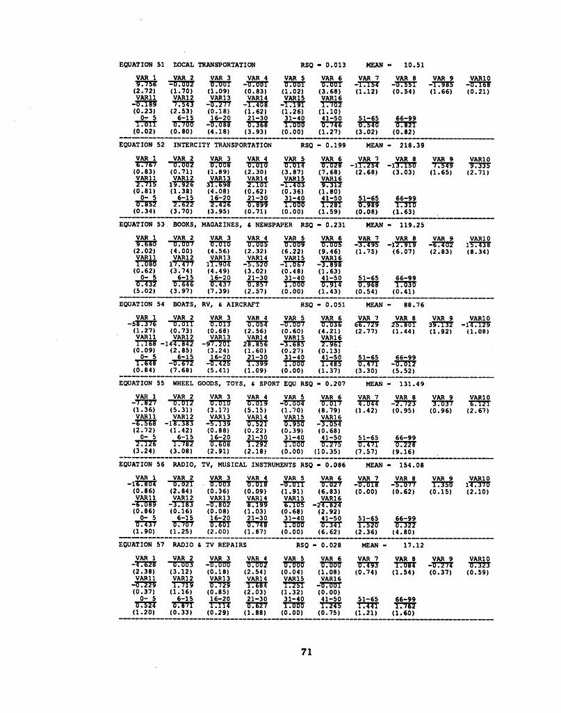
EQUATION 51 LOCAL TRANSPORTATION RSQ - 0 .0 1 3 MEAN 1 0 .5 1

VAR 1 VAR 2 VAR 3 VAR 4 VAR 5 VAR 6 VAR 7 VAR 8 VAR 9 VAR107 7 7 5 7 - 6.£>02 O .o o i - t ) . o f l l 6 . 6o i 0 . 60 I -1 .1 5 4 -0 1 5 5 1 -1 .9 8 5 - 6.168(2 .7 2 ) (1 .7 0 ) (1 .0 9 ) (0 .8 3 ) ( 1 . 02 ) (3 .6 8 ) ( 1 . 12) (0 .5 4 ) ( 1 . 66 ) ( 0 . 21 )VAR11 VAR12 VAR13 VAR14 VAR15 VAR16

-0 .1 8 9 7 .5 4 3 -*57277 -1 .4 0 8 -1 .1 5 1 1 .7 0 2(0 .2 3 ) (2 .5 3 ) (0 .1 8 ) (1 .6 2 ) (1 .2 6 ) ( 1 . 10 )

O f 5 6 -1 5 16 -2 0 2 1 -3 0 3 1 -4 0 41 -5 0 5 1 -6 5 6 6 -9 9T 7 7 T T d . lo d -O .b s s 0 .3 6 8 1.066 7 7 m 0 .5 4 0 0 .B 21(0 . 02 ) (0 .8 0 ) (4 .1 8 ) (3 .9 3 ) ( 0 . 00 ) (1 .2 7 ) (3 .0 2 ) (0 .8 2 )

EQUATION 52 INTERCITY TRANSPORTATION RSQ - 0 .1 9 9 MEAN - 2 1 8 .3 9

VAR 1 VAR 2 VAR 3 VAR 4 VAR 5 VAR 6 VAR 7 VAR 8 VAR 9 VAR10T T 7 5 7 d .002 t i.0 0 8 0.010 6 .0 1 4 0 .0 2 8 -1 T 7 7 5 T -1*37157 7 7 5 7 7 7 7 3 3 7(0 .8 3 ) (0 .7 1 ) (1 .8 9 ) (2 .3 0 ) (3 .8 7 ) (7 .6 8 ) (2 . 68 ) (3 .0 3 ) (1 .6 5 ) (2 .7 1 )VAR11 VAR12 VAR13 VAR14 VAR15 VAR162 .7 1 5 1 ^ .9 2 6 3 l . 6^8 2 . 1o i —1 .40 3 7 7 3 7 7

(0 .8 1 ) (1 .3 8 ) (4 .0 8 ) (0 .6 2 ) (0 .3 6 ) (1 .8 0 )0 - 5 6 -1 5 1 6 -2 0 2 1 -3 0 3 1 -4 0 4 1 -5 0 5 1 -6 5 6 6 -9 9

7 7 5 7 7 2 .6 2 2 2 .4 2 6 0 .8 9 9 1.660 T 7 7 5 T 7 7 5 7 7 T 7 3 T 7(0 .3 4 ) (3 .7 0 ) (3 .9 5 ) (0 .7 1 ) (0 . 00 ) (1 .5 9 ) (0 .0 8 ) (1 .6 3 )

EQUATION 53 BOOKS, MAGAZINES, & NEWSPAPER RSQ - 0 .2 3 1 MEAN - 1 1 9 .2 5

VAR 1 VAR 2 VAR 3 VAR 4 VAR 5 VAR 6 VAR 7 VAR 8 VAR 9 VAR10T 7 T 5 7 f l.O o / 7 7 7 T 7 6 . 00b 7 7 7 7 ? 6 . 005 -TTTSF —17 7517 -T T T 7 7 177737(2 . 02) (4 .0 0 ) (4 .5 6 ) (2 .3 2 ) ( 6 . 22 ) (9 .4 6 ) (1 .7 5 ) (6 .0 7 ) (2 .8 3 ) (8 .3 4 )V A R ll VAR12 VAR13 VAR14 VAR15 VAR161 .0 8 0 lT .4 7 7 1T757T -7 7 5 7 7 -1 .0 6 7 -T755TT

(0 .6 2 ) (3 .7 4 ) (4 .4 9 ) (3 .0 2 ) (0 .4 8 ) (1 .6 3 )0 - 5 6 -1 5 1 6 -2 0 21 -3 0 3 1 -4 0 4 1 -5 0 5 1 -6 5 6 6 -9 9

0 .4 3 2 6 . 646 6 .4 3 7 0 .8 5 7 1.666 6 .9 1 4 0 .9 6 8 1 .6 3 b(5 .0 2 ) (3 .9 7 ) (7 .3 9 ) (2 .5 7 ) ( 0 . 00 ) (1 .4 3 ) (0 .5 4 ) (0 .4 1 )

EQUATION 54 BOATS, RV, fi AIRCRAFT RSQ - 0 .0 5 1 MEAN 8 8 .7 6

VAR 1 VAR 2 VAR 3 VAR 4 VAR 5 VAR 6 VAR 7 VAR 8 VAR 9 VAR10-5 7 T 3 7 6 ■"0V0I 1 7 7 7 T 7 0 . 054 -7 7 7 7 7 6 . 036 677777 2 5 .B01 3 9 .1 3 2 -1 4 .1 2 9

(1 .2 7 ) (0 .7 3 ) (0 . 68 ) (2 .5 6 ) (0 .6 0 ) (4 .2 1 ) (2 .7 7 ) (1 .4 4 ) (1 .9 2 ) (1 .0 8 )V A R ll VAR12 VAR13 VAR14 VAR 15 VAR16T 7 T 7 7 - 1 4 4 .84 2 - 9 ^.201 2 6 .8 5 6 —3 . 665 TTTTT(0 .0 9 ) (2 .8 5 ) (3 .2 4 ) (1 .6 0 ) (0 .2 7 ) (0 .1 3 )

0 - 5 6 -1 5 1 6 -2 0 2 1 -3 0 3 1 -4 0 41 -5 0 5 1 -6 5 6 6 -9 9T 7 7 7 7 -*77777 -TTT777 T 7 3 7 7 T 7 7 7 7 Y .4 8 5 0 .4 7 1 -7 7 5 7 7(0 .8 4 ) (7 .6 8 ) (5 .4 1 ) (1 .0 9 ) (0 . 00 ) (1 .3 7 ) (3 .3 0 ) (5 .5 2 )

EQUATION 55 WHEEL GOODS, TOYS!, & SPORT' EQU RSQ - 0 .2 0 7 MEAN - 1 3 1 .4 9

VAR 1 VAR 2 VAR 3 VAR 4 VAR 5 VAR 6 VAR 7 VAR 8 VAR 9 VAR10-7 7 5 7 7 0.012 0 .0 1 0 0 .0 1 9 —0 .004 0 .0 1 7 4 .044 -77777 *37737 6.121(1 .3 6 ) (5 .3 1 ) (3 .1 7 ) (5 .1 5 ) (1 .7 0 ) (8 .7 9 ) (1 .4 2 ) (0 .9 5 ) (0 .9 6 ) (2 .6 7 )V A R ll VAR12 VAR13 VAR14 VAR15 VAR16

—6 . S 6& - l f e . 383 -3 7 m *77777 0 .9 5 0 -TT75T(2 .7 2 ) (1 .4 2 ) ( 0 . 88 ) ( 0 . 22 ) (0 .3 9 ) ( 0 . 68 )

0 - 5 6 -1 5 1 6 -20 2 1 -3 0 3 1 -4 0 41 -5 0 5 1 -6 5 6 6 -9 92 .1 2 6 1 .7 8 2 0 . <>08 1.242 1.000 77275 *0 7 1 0 .2 2 8

(3 .2 4 ) (3 .0 8 ) (2 .9 1 ) (2 .1 8 ) ( 0 . 00 ) (1 0 .3 5 ) (7 .5 7 ) (9 .1 6 )

EQUATION 56 RADIO, TV, MUSICAL INSTRUMENTS RSQ - 0 .0 8 6 MEAN - 1 5 4 .0 8

VAR 1 VAR 2 VAR 3 VAR 4 VAR 5 VAR 6 VAR 7 VAR 8 VAR 9 VAR10- 1 ^ .8 0 4 "0.021 6 .0 0 3 6 .0 1 8 -77777 77777 - 6 . d ie -77777 T7357 1 4 .3 7 0

(0.86) ( 2 .8 4 ) (0 .3 6 ) (0 .0 9 ) (1 .9 1 ) (6 .8 3 ) (0.00) (0 .6 2 ) (0 .1 5 ) (2.10)V A R ll VAR12 VAR13 VAR14 VAR15 VAR16

-6 .0 8 9 -TTT57 -6 .8 0 2 8 .1 9 9 6.10S ■-277577(0.86) ( 0 .1 6 ) (0 .0 8 ) (1 .0 3 ) (0.68) ( 2 .9 2 )

0 - 5 6 -1 5 1 6 -2 0 2 1 -3 0 3 1 -4 0 4 1 -5 0 5 1 -6 5 6 6 -9 90.431 0 .7 0 7 f l . £ o i 77777 1.000 "77377 '1.520 6 .3 2 2

(1 .9 0 ) (1 .2 5 ) (2 . 00 ) (1 .8 7 ) ( 0 . 00 ) (6 .6 2 ) (2 .3 6 ) (4 .8 0 )

EQUATION 57 RADIO & TV REPAIRS RSQ - 0 .0 2 8 MEAN - 1 7 .1 2

VAR 1 VAR 2 VAR 3 VAR 4 VAR 5 VAR 6 VAR 7 VAR 8 VAR 9 VAR10-4.&2B 0 .0 0 3 —0 .Gob 0.002 77777 77777 77793 Y.084 -77777' 0 .3 2 3(2 .3 8 ) (3 .1 2 ) (0 .1 8 ) (2 .5 4 ) (0 .0 4 ) (1 .0 8 ) (0 .7 4 ) (1 .5 4 ) (0 .3 7 ) (0 .5 9 )V A R ll VAR12 VAR13 VAR14 VAR15 VAR16

-77777 1.715 0.725 T7777 TT777 -*77771(0 .3 7 ) (1 .1 6 ) (0 .8 5 ) (2 .0 3 ) (1 .3 2 ) (0.00)

0 - 5 6 -1 5 16 -2 0 2 1 -3 0 3 1 -4 0 4 1 -5 0 5 1 -6 5 6 6 -9 96 .5 2 4 757577 i . 114 77777 1.006 T7377 T777T T7777

(1.20) ( 0 .3 3 ) (0 .2 9 ) (1.88) (0.00) (0 .7 5 ) (1.21) ( 1 .6 0 )

71

EQUATION 58 FEES 6 ADMISSIONS RSQ - 0 .3 7 5 MEAN 2 2 9 .9 4

VAR 1 VAR 2 VAR 3 VAR 4 VAR 5 VAR 6-1 0 .2 8 2 "0.015 77777 0 .0 1 7 77737 77777

(1 .1 6 ) (4 .6 8 ) (5 .0 8 ) (3 .5 9 ) (7 .7 8 ) (1 3 .4 3 )V A R ll VAR12 VAR13 VAR14 VAR15 VAR16

-4 .0 0 2 -4 8 .9 1 6 - lT r ra r 6 .0 0 5 -TT T 5 -77177(1 .1 4 ) (3 .2 4 ) (2 .2 8 ) (1 .6 3 ) (1 .1 7 ) (0 .0 3 )

0 - 5 6 -1 5 1 6 -2 0 2 1 -3 0 3 1 -4 0 4 1 -5 0& .5 i6 TTTS? b . 782 ■077 i . o o b 0 .8 6 9

(3 .1 5 ) (4 .2 2 ) (2 .2 4 ) (4 .1 7 ) (0 .0 0 ) (2 .0 0 )

VAR 7 -1 .3 9 2 (0 .3 3 )

5 1 -6 50 .6 9 8

(5 .5 6 )

VAR 8-16.172

(4 .1 3 )

6 6 -9 90 .7 7 6

(3 .0 8 )

VAR 97775T

(0 .1 6 )

VAR10377573(8 .0 6 )

EQUATION 59 OTHER REC SUPPLIES, EQUIPMENT RSQ - 0 .2 1 3 MEAN - 2 0 4 .8 0

VAR 1 VAR 2 VAR 3 VAR 4 VAR 5 VAR 6 VAR 7 VAR 8 VAR 9 VAR10—377377 _7: 022 "0.027 77717 77777 0 .0 1 6 -2.546 77777 277T77 1T7B7T(2.63) (5 .16 ) (4 .46) (2 .32 ) (6.45) (8 .83 ) (0 .47) (0 .15 ) (3 .55 ) (2 .69 )V A R ll VAR12 VAR13 VAR14 VAR15 VAR16-T7777 - l6 . <351 1 6 .621 8 .3 1 7 1 5 .8 6 6 -77737

(0 .30 ) (0 .9 9 ) (1 .9 5 ) (1 .6 9 ) (2 .80) (0 .5 6 )0 - 5 6 -1 5 1 6 -2 0 2 1 -3 0 3 1 -4 0 4 1 -5 0 5 1 -6 5 6 6 -9 977777 775T7 b.74 6 0 .7 9 1 1 .boo 0 .6 5 8 0 .6 4 1 0 . 441

(5 .87 ) (1 .6 4 ) (2 .65) (3 .47 ) (0 .0 0 ) (5 .6 5 ) (6 .6 7 ) (9 .3 0 )

EQUATION 60 EDUCATION RSQ - 0 .2 2 6 MEAN - 2 1 3 .0 7

VAR 1 VAR 2 VAR 3 VAR 4 VAR 5 VAR 6 VAR 7 VAR 8 VAR 9 VAR10-1 .4 2 8 ” 0:001 77707 77707 77073 5.001 -1 .4 4 1 -1 .2 0 2 -77377 7.791(0 .5 1 ) (0 .58 ) (0 .6 1 ) (0 .6 0 ) (0 .6 1 ) (0 .6 1 ) (0 .5 9 ) (0 .58 ) (0 .6 0 ) (0 .6 1 )V A R ll VAR12 VAR13 VAR14 VAR15 VAR16 ,

- 0 .6 3 8 -177537 - '7 .4 3 1 1 .9 4 2 77177 -77T57(0 .5 1 ) (0 .6 1 ) (0 .6 1 ) (0 .5 9 ) (0 .15) (0 .21 )

0 - 5 6 -1 5 1 6 -2 0 2 1 -3 0 3 1 -4 0 4 1 -5 0 5 1 -6 5 6 6 -9 9T7T77 2 fa .581 237777 T773T 1 .00 0 177757 177707 - 0 .3 4 5(0 .22 ) (0 .5 7 ) (0 .5 8 ) (0 .5 2 ) (0 .00) ( 0 .5 9 ) (0 .5 6 ) (0 .8 3 )

EQUATION 61 CASH CONTRIBUTION RSQ - 0 .2 3 0 MEAN - 4 4 1 .1 3

VAR 1 VAR 2 VAR 3 VAR 4 VAR 5 VAR 6 VAR 7 VAR 8 VAR 9 VAR10-277757 d . o i v 77717 777T7 77073 77077 2 8 .6 2 9 2 1 .7 8 2 177777 477075'(1 .3 0 ) (2 .5 4 ) (2 .0 6 ) (2 .3 1 ) (4 .1 1 ) (6 .11 ) (3 .3 9 ) (2 .7 6 ) (1 .7 8 ) (4 .9 2 )V A R ll VAR12 VAR13 VAR14 VAR15 VAR16

—11 .1 0 6 -2 9 .4 8 7 -2777577 -T777T -277757 ”77751(1 .6 0 ) (2 .1 7 ) (3 .0 7 ) (0 .2 4 ) (2 .0 9 ) (0 .9 3 )

0 - 5 6 -1 5 1 6 -2 0 2 1 -3 0 3 1 -4 0 4 1 -50 5 1 -6 5 6 6 -9 91 .3 4 4 0 .9 9 5 77377 77733 T7070 T7757 77377 5 .4 7 0

72

TABLE 2.3

E ffe ct o f Dem ographic Variables

REGION EDUCATION WORKING FAMILY AGESPOUSE SIZE

N .C . S. W. COLLEGE YES 1 2 5+ 3 5 - 55+

1 . FOOD, OFF PRE ( - ) (-> ( - ) <-) < -) (+ ) ( + )

2 . FOOD, ON PREM (+)

3 . ALCOHOL, OFF ( - ) ( - ) (+ ) (+ ) ( - )

4 . ALCOHOL, ON P ( - ) ( - ) (+) (+)

5 . TOBACCO PRODU ( - ) ( - ) ( - ) ( - ) <+) (+) ( - )

6 . SHOES & FOOTW ( - ) (+) (+) {+) ( - )

7 . WOMEN'S & CHI <-) (+) (+) ( - )

8 . MEN'S & BOY'S ( - ) <-) (+) <-) < -) { - ) (+)

9 . LUGGAGE

1 0 . JEWELRY & WAT (-> (+)

1 1 . LAUNDRIES, ST ( - ) ( - ) <-) (+) (+) (+) ( - ) (+)

1 2 . OTHER JEWELRY (+) ( - )

1 3 . PERSONAL CARE (+)

14 . OWNER-OCCUPIE ( - ) ( - ) (+)

1 5 . TENANT-OCCUPI ( - ) ( - ) < -) (+) (+) ( - ) (+ ) ( - )

1 6 . OTHER HOUSING

1 7 . ADDITIONS, AL

1 8 . HOTELS & MOTE ( - ) ( - ) (+) (+ ) ( - )

1 9 . FURNITURE ( - ) ( - )

2 0 . KITCHEN & HOU (+) (+) (+) (+)

2 1 . CHINA, GLASSW (+) (+) ( - ) ( - )

2 2 . OTHER DURABLE (+) (+ ) (+)

2 3 . FLOOR COVERIN

2 4 . SEMIDURABLE H (+) (+) ( - ) ( - )

73

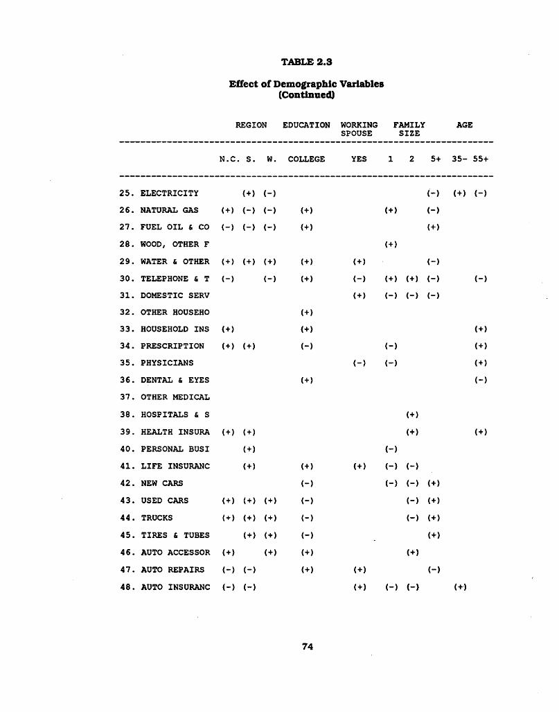
E ffe ct o f Dem ographic Variables (C ontinued)

TABLE 2.3

REGION EDUCATION WORKING FAMILY AGESPOUSE SIZE

N .C . S. w. COLLEGE YES 1 2 5+ 3 5 - 55+

2 5 . ELECTRICITY ( + ) ( - ) (-> ( + ) ( - )

2 6 . NATURAL GAS ( + ) ( - ) ( - ) (+) (+) ( - )

2 7 . FUEL O IL & CO (-> ( - ) ( - ) (+> (+>

2 8 . WOOD, OTHER F ( + )

2 9 . WATER & OTHER ( + ) ( + ) (+) (+> ( + ) <-)

3 0 . TELEPHONE & T ( - ) <-) (+) ( - ) (+) <+) ( - ) ( - )

3 1 . DOMESTIC SERV ( + ) ( - ) ( - ) ( - )

32 . OTHER HOUSEHO (+)

3 3 . HOUSEHOLD INS < + ) (+) ( + )

3 4 . PRESCRIPTION ( + ) ( + ) ( - ) ( - ) ( + )

3 5 . PHYSICIANS ( - ) ( - ) ( + )

3 6 . DENTAL & EYES (+) ( - )

3 7 . OTHER MEDICAL

38 . HOSPITALS & S (+)

39 . HEALTH INSURA ( + ) ( + ) (+) ( + )

40 . PERSONAL BUSI ( + ) ( - )

4 1 . L IF E INSURANC ( + > (+) ( + ) ( - ) ( - )

42 . NEW CARS ( - ) ( - ) ( - ) (+)

43 . USED CARS ( + ) ( + ) (+) ( - ) ( - ) (+)

4 4 . TRUCKS ( + ) ( + ) (+) (-) (-) (+)

4 5 . TIRES & TUBES (+) (+) (-) (+>4 6 . AUTO ACCESSOR ( + ) (+) (+) <+>

4 7 . AUTO REPAIRS (-) (-) (+) ( + ) (-)

4 8 . AUTO INSURANC (-) (-) ( + ) (-) (-) (+)

74

E ffe ct o f Dem ographic Variables (C ontinued)

TABLE 2.3

REGION EDUCATION WORKING FAMILY AGESPOUSE SIZE

N .C . £ w. COLLEGE YES 1 2 5+ 3 5 - 55+

4 9 . GASOLINE & 01 ( + ) ( + ) ( + ) (-> < + > ( - ) ( + ) ( - )

5 0 . TOLLS, PARKIN <--> (+) ( + )

51 . LOCAL TRANSPO <-) (+)

5 2 . INTERCITY TRA ( - ) <-■) (+) (+) (+) ( + )

5 3 . BOOKS, MAGAZI ( - ) <--> ( - ) ( + ) ( + ) (+) ( - )

5 4 . BOATS, RV, & < + > (+) (-) (-)

5 5 . WHEEL GOODS, ( + ) ( - )

56 . RADIO, TV, RE ( + ) ( - )

5 7 . REPAIRS, RADI <+ >

5 8 . FEES & ADMISS <--) ( + ) ( - ) ( - )

5 9 . OTHER RECREAT <+) ( + ) (+) (+) ( + )

60 . EDUCATION

6 1 . CASH CONTRIBU ( + ) < + ) ( + > ( + ) (-) (-) (-)

75

NoudnnsN

oo N

oiidnnsNO

O

FIGURE 2.2

P lo t o f Engel Curves

EQ 1. FOOD. OFF PREMISE

(ThouMnda)

EQ 2. FOOD. ON PREMISE

(ThouMnda)

EQ 3. ALCOHOL OFF PREMISE

(ThauMndg

EQ 4. ALCOHOL, ON PREMISE

(Thounnda)

EQ 5. TOBACCO

(ThouM nd^

EQ 6. SHOES AND FOOTWEAR

(Thousand^

76

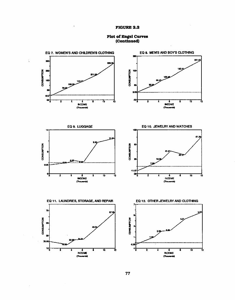
CONS

UMPT

ION

CONS

UMPT

ION

FIGURE 2.2

P lo t o f Engel Curves (C ontinued)

EQ 7. WOMEN’S AND CHILDREN’S CLOTHING EQ8. MEN’S AND BOY'S CLOTHING

(Thousand̂ (ThouMnda)

EQ 9. LUGGAGE

(TKou»«ndO

EQ 1 0. JEWELRY AND WATCHES

(B n u w n ji)

EQ 11. LAUNDRIES, STORAGE. AND REPAIR

(ThouMndg

EQ 12. OTHER JEWELRY AND CLOTHING

(Thounndt)

77

FIGURE 2.2

P lo t o f Engel Curves (C ontinued)

EQ 13. PERSONAL CARE EQ14. OWNER-OCCUPIED HOUSING

(Thousand^ (ThouMnda}

EQ 15. TENANT-OCCUPED HOUSING EQ 16. OTHER HOUSING

(Thouxnd^ (Tham m di)

EQ 1 8. HOTELS AND MOTELS EQ 19. FURNITURE

(Ito u M n d ^ (ThouMnda)

78

CONS

UMPT

ION

CONS

UMPT

ION

P lo t o f Engel Curves (C ontinued)

FIGURE 2.2

EQ 20. KITCHEN AND HOUSEHOLD APPLIANCE EQ 21. CHINA. GLASSWARE. AND TABLEWARE

(TheuMnd̂ (ThouMnda)

EQ 22. OTHER DURABLE HOUSE FURNISHINGS EQ23l FLOOR COVERINGS

(ThouMnd̂ (ThouMnda)

EQ 24. SEMIDURABLE HOUSE FURNISHINGS EQ 25. ELECTRICITY

(Thoueen*4 (ThouM ndf

79

CONS

UMPT

ION

P lo t o f Engel Curves (C ontinued)

FIGURE 2.2

EQ 26. NATURAL GAS EQ 27. FUEL OIL AND COAL

(Thounnd^ (TheuMnd4

EQ 28. WOOD. OTHER FUEL, AND TANK GAS

(ThouMnJi)

EQ 29. WATER AND OTHER SANITARY

(Thousand))

EQ 3a TELEPHONE AND TELEGRAPH

(D auN ndA

EQ 31. DOMESTIC SERVICE

(Thounnd^

80

NO

lidWnSN

CO

P lo t o f Engel Curves (C ontinued)

FIGURE 2.2

EQ 32. OTHER HOUSEHOLD OPERATIONS EQ 33. HOUSEHOLD INSURANCE

(T haam k) (lhomwd<

EQ 34. PRESCRIPTION DRUG AND SUNDRES EQ 35. PHYSICIANS

(ThouMnda) (ThouMnd̂

EQ 36. DENTAL AND EYES EQ 37. OTHER MEDICAL SERVICES

(Thou—nd^ (Thou—nd̂

81

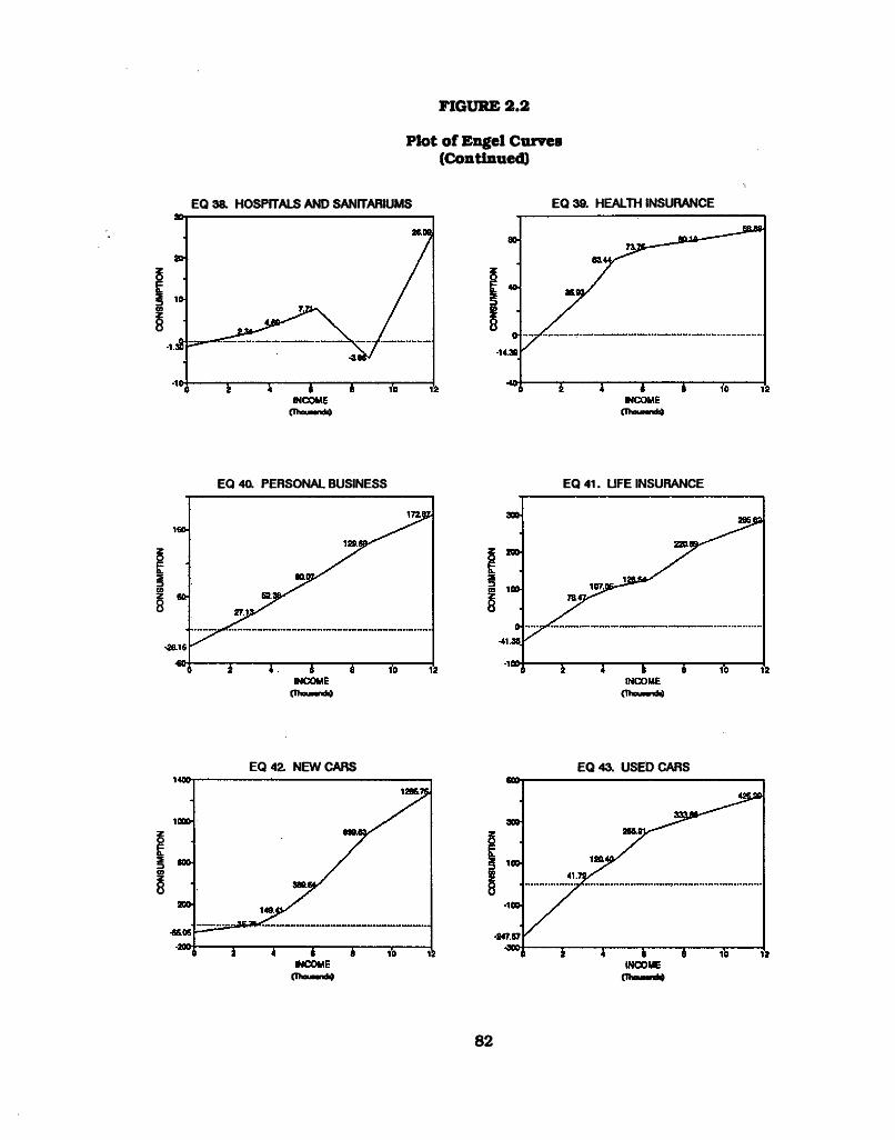
NO

iidnnsNO

O

NO

iidnnsNO

O

P lo t o f Engel Curves (C ontinued)

FIGURE 2.2

EQ 38. HOSPITALS AND SANITARIUMS EQ 38. HEALTH INSURANCE

(ThouMndti (Thounnda)

EQ 40l PERSONAL BUSINESS EQ 41. UFE INSURANCE

(IhouNnd̂ (ThouMndt)

EQ 42. NEW CARS EQ 43l USED CARS

(TheuMnd̂ (Thounnd^

82

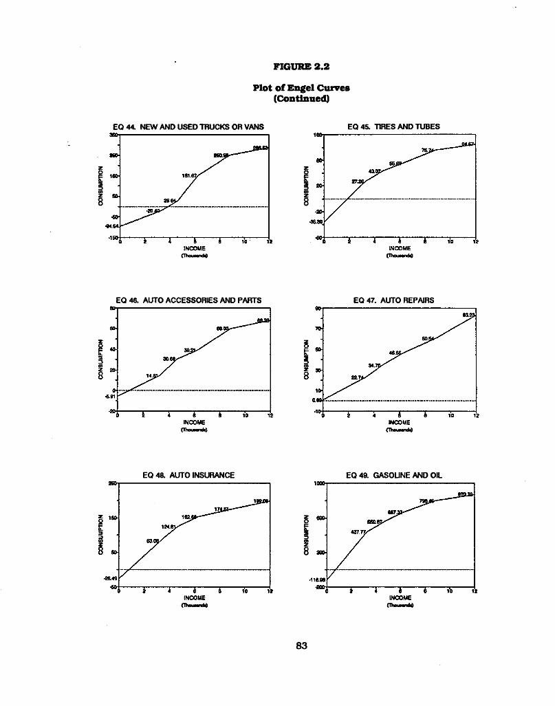
P lo t o f Engel Curves (C ontinued)

FIGURE 2.2

EQ 44. NEW AND USED TRUCKS OR VANS EQ 45. TIRES AND TUBES

(Thounnd^ (ThouMndg

EQ 46. AUTO ACCESSORES AND PARTS

(ThouMnd̂

EQ 48. AUTO INSURANCE

(Thouaandg

EQ 47. AUTO REPAIRS

(ThouMnd̂

EQ49. GASOUNE AND OIL

(ThouMnda)

83

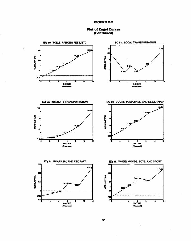
CONS

UMPT

ION

CONS

UMPT

ION

P lo t o f Engel Curves (C ontinued)

FIGURE 2.2

EQ Sa TOLLS, PARKING FEES. ETC EQ 51. LOCAL TRANSPORTATION

(Thom Tuk) (ThouMncfa)

EQ 52. INTERCITY TRANSPORTATION EQ 53. BOOKS. MAGAZINES. AND NEWSPAPER

(ThouMnda) (ThouMndO

EQ 54. BOATS. RV. AND AIRCRAFT EQ 55. WHEEL GOODS. TOYS. AND SPORT

(ThouM ndt) (T ham nd^

84

P lo t o f Engel Curves (C ontinued)

FIGURE 2.2

EQ 56. RADIO. TV, RECORDERS EQ 57. RADIO AND TV REPAIRS AND RENTAL

(IhauwnJj (IhouMnd̂

EQ 58. FEES AND ADMISSIONS EQ 59. OTHER RECREATIONAL SUPPUES

(Thouw n*) (ThouM n*)

EQ 60. EDUCATION EQ 61. CASH CONTRIBUTION

(TheuMnd̂ (TheuMnd4

85

ADUL

T EQ

UIVA

LENC

Y W

EIGHT

AD

ULT

EQUI

VALE

NCY

WEIG

HT

ADUL

T EQ

UIVA

LENC

Y

FIGURE 2.3

Bar C hart o f A d u lt E quivalency W eights

EQ 1. FOOD, OFF PREMISE

AGE GROUP

EQ 2. FOOD. ON PREMISE

AGE GROUP

EQ & ALCOHOL, OFF PREMISE EQ 4. ALCOHOL, ON PREMISEi.2i

ae-

0.6-

a<-

02-ao7

JZL

a 46

1

aso

i

1.00

aei

I

0.68

I0-6 6-16 16-20 21-30 31-40 41-60 61-66 66-99

AGE GROUP

1. i.2i i 11 ^ £ 06-

| <U-auj 0.21

o-•0-M •ai9

a 78

I

1.14

1

1.00

0S7

I

0-6 6-16 16-20 21-30 31-40 41-60 61-66 66-99 AGE GROUP

EQ 5. TOBACCO

AGE GROUP

EQ 6. SHOES AND FOOTWEAR

AGE GROUP

86

ADUL

T EQ

UIVA

LENC

Y W

EIGHT

AD

ULT

EQUI

VALE

NCY

WEIG

HT

ADUL

T EQ

UIVA

LENC

Y W

EIGH

T

FIGURE 2.3

Bar Chart of Adult Equivalency Weights(Continued)

EQ 7. WOMEN’S AND CHILDREN’S CLOTHING EQ & MEN’S AND BOY’S CLOTHING

EQ 9. LUGGAGE EQ 10. JEWELRY AND WATCHES

0-6 6-16 16-20 21-30 31-40 41-60 61-66 66-99 AGE GROUP

EQ 11. LAUNDRIES, STORAGE, AND REPAIR EQ 1Z OTHER JEWELRY AND CLOTHING

87

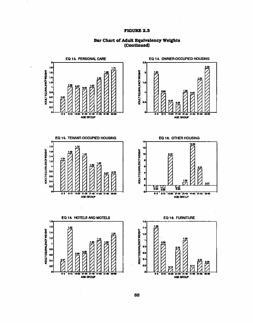
FIGURE 2.3

Bar Chart of Adult Equivalency Weights(Continued)

EQ 1 a PERSONAL CARE EQ 14. OWNER-OCCUPIED HOUSING

EQ 15. TENANT-OCCUPIED HOUSING EQ 1& OTHER HOUSING

EQ 18. HOTELS AND MOTELS

AGE GROUP

EQ 19. FURNITURE

AGE GROUP

ADUL

T EQ

UIVA

LENC

Y W

EIGHT

AD

ULT

EQUI

VALE

NCE

WEIG

HT

ADUL

T EQ

UIVA

LENC

Y W

EIGH

T

FIGURE 2.3

Bar Chart of Adult Equivalency Weights(Continued)

EQ 20. KITCHEN AND HOUSEHOLD APPLIANCE EQ 21. CHINA, GLASSWARE, AND TABLEWARE

EQ 22. OTHER DURABLE HOUSE FURNISHINGS EQ 23. FLOOR COVERINGS»■

i % *

i * in5 " 9 »

•1-

4.99

1.60

I

100 A-K 0199f t vx

■0.1S

AGE GROUP

EQ 24. SEMIDURABLE HOUSE FURNISHINGS

AGE GROUP

EQ2& ELECTRICITY

AGE GROUP

89

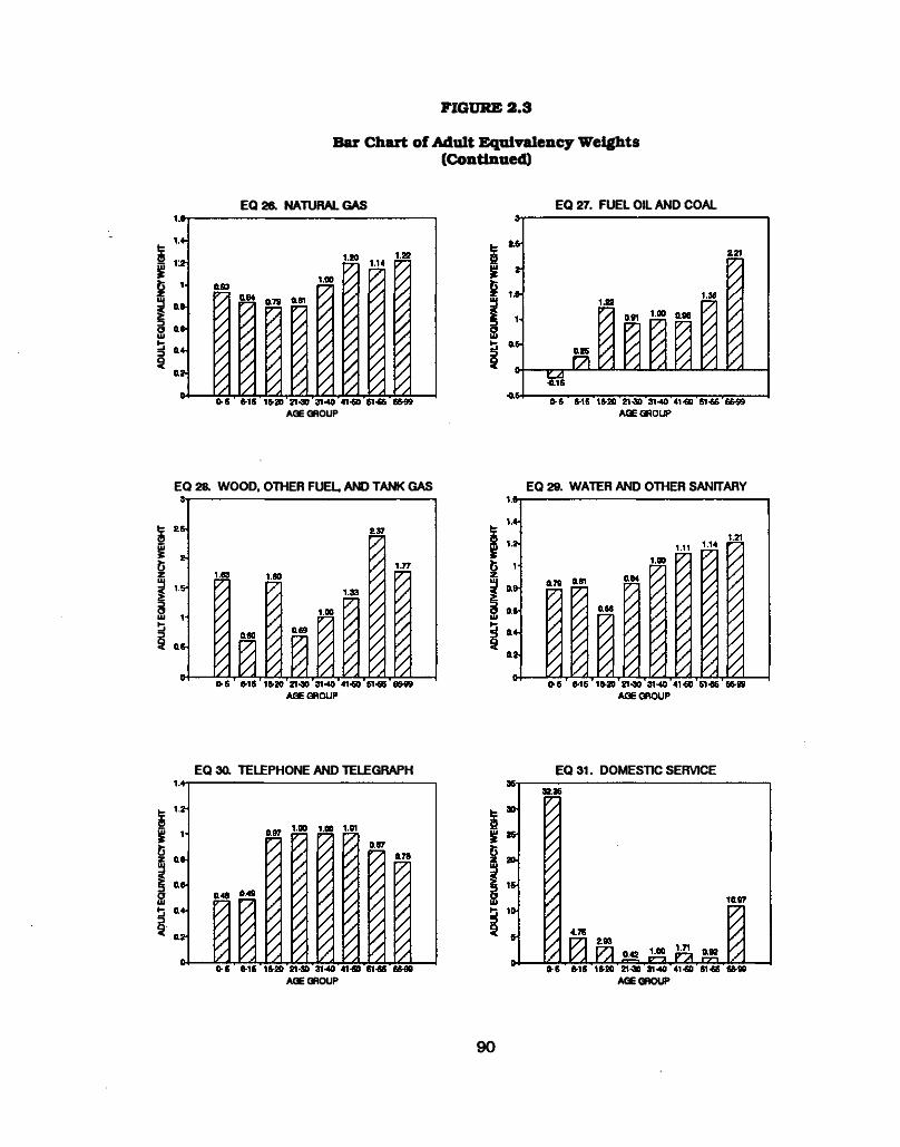
ADUL

T EQ

UIVA

LENC

Y W

EIGHT

AD

ULT

EQUI

VALE

NCY

WEIG

HT

ADUL

T EQ

UIVA

LENC

Y

FIGURE 2.3

Bar Chart of Adult Equivalency Weights(Continued)

EQ 26. NATURAL GAS

AGE GROUP

EQ 27. FUEL OIL AND COAL

EQ 28. WOOD, OTHER FUEL, AND TANK GAS EQ 29. WATER AND OTHER SANITARY

EQ 3a TELEPHONE AND TELEGRAPH

AGE GROUP

EQ 31. DOMESTIC SERVICE

AGE GROUP

90

ADUL

T EQ

UIVA

LENC

Y W

EIGHT

AD

ULT

EQUI

VALE

NCY

WEIG

HT

ADUL

T EQ

UIVA

LENC

Y

FIGURE 2.3

Bar Chart of Adult Equivalency Weights(Continued)

EQ 32. OTHER HOUSEHOLD OPERATIONS EQ 3a HOUSEHOLD INSURANCE

EQ 34. PRESCRIPTION DRUG AND SUNDRIES *i

0-6 6-16 16-20 21-30 31-40 41-60 61-66 AGE GROUP

EQ 35. PHYSICIANS

EQ 36. DENTAL AND EYES

AGE GROUP AGE GROUP

91

FIGURE 2.3

Bar Chart of Adult Equivalency Weights(Continued)

EQ 38. HOSPITALS AND SANITARIUMS EQ 39. HEALTH INSURANCElo­s­s'7-

*s-4-

»5- 1- 0-

aesXZL

4.66

&S4

1.46

Z2 E2L0-6 6-16 16-20 21-30 31-40 41-60 61-66 6649

AGE GROUP

EQ 40. PERSONAL BUSINESS EQ 41. LIFE INSURANCE

EQ 42. NEW CARS

AQE GROUP

EQ 43. USED CARS

AGE GROUP

92

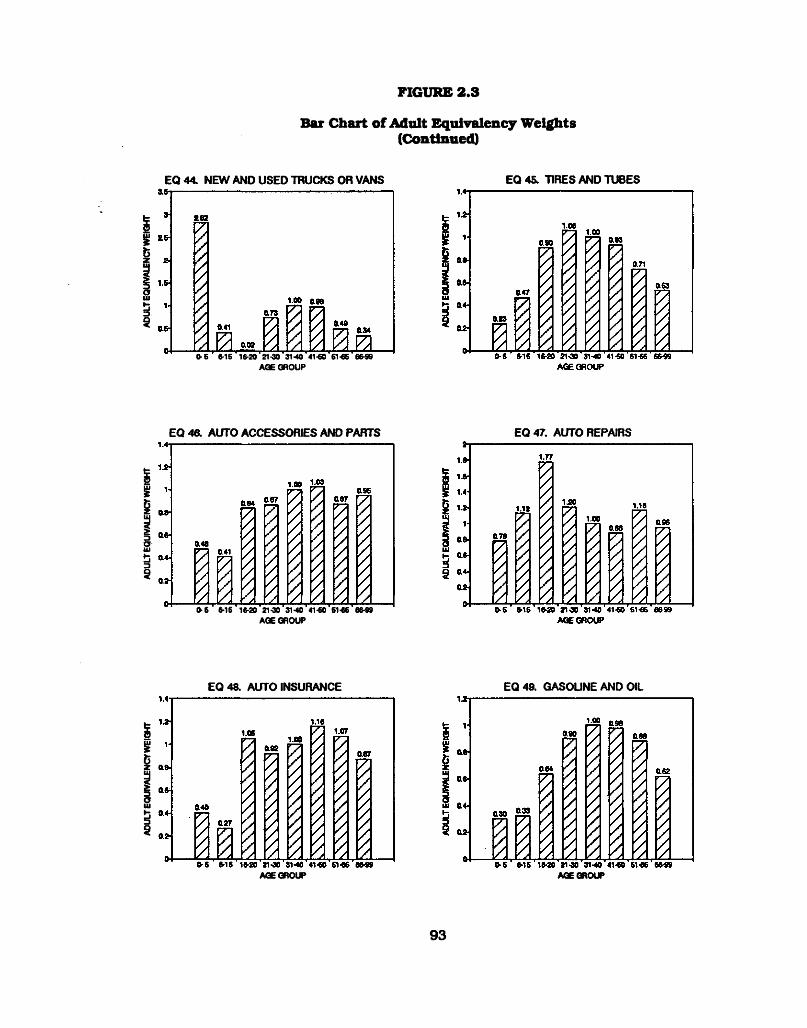
ADUL

T EQ

UIVA

LENC

Y W

EIGHT

AD

ULT

EQUI

VALE

NCY

WEIG

HT

ADUL

T EQ

UIVA

LENC

Y W

EIG

HT

FIGURE 2.3

Bar Chart of Adult Equivalency Weights(Continued)

EQ 44. NEW AND USED TRUCKS OB VANS EQ 45. TIRES AND TUBES

6-16 16-20 21-30 31-40 41-60 61-66 6649 AGE GROUP

EQ 46. AUTO ACCESSORIES AND PARTS

0-6 6-16 16-20 21-30 31-40 41-60 61-66 66-99 AGE GROUP

EQ 47. AUTO REPAIRS

EQ 48. AUTO INSURANCE

AGE GROUP

EQ 49. GASOLINE AND OIL

AGE GROUP

93

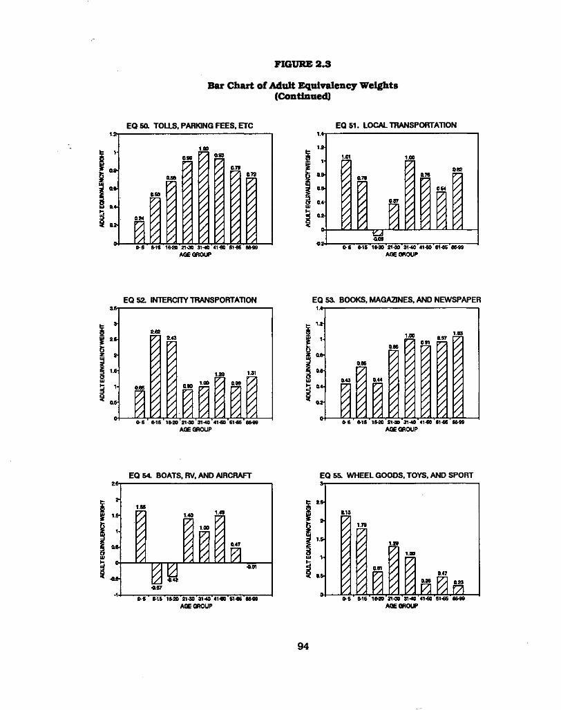
FIGURE 2.3

Bar Chart of Adult Equivalency Weights(Continued)

EQ 5a TOLLS, PARKING FEES, ETC EQ 51. LOCAL TRANSPORTATION

EQ 52. INTERCITY TRANSPORTATION

16-20 21-30 31-40 41-GO 61-66 6649 AGE GROUP

EQ 53. BOOKS, MAGAZINES, AND NEWSPAPER

EQ 54. BOATS. RV, AND AIRCRAFT

AGE GROUP

EQ 55. WHEEL GOODS. TOYS. AND SPORT

AGE GROUP

ADUL

T EQ

UIVA

LENC

Y W

EIGHT

AD

ULT

EQUI

VALE

NCY

WEIG

HT

ADUL

T EQ

UM

FIGURE 2.3

Bar Chart of Adult Equivalency Weights(Continued)

EQ 5& RADIO. TV, RECORDERS EQ 57. RADIO AND TV REPAIRS AND RENTAL

EQ 58. FEES AND ADMISSIONS EQ 58. OTHER RECEATIONAL SUPPLIES

EQ 60l EDUCATION

AGE GROW

EQ 61. CASH CONTRIBUTION

AGE GROUP

95

E stim ated C oefficients by the B ig -T icke t-Item A nalysis

TABLE 2.4

E q u a tio n 1 . Food , O f f P rem ise 1 2 . Food, On P rem ise

Ind epe nde n t L e a s t Le as t I L e a s t Le as tV a r ia b le P ro b it S q u a re s l Squares2 1 P ro b it S q u a re s l Squares2

In te r c e p t 362.5991 363.2742 362 .4836 1 -3 9 .0 7 9 9 -4 4 .3 9 9 4 -2 2 .2 7 6 4

In co m e ( $ ) :0-3310 0 .2 259 0 .2 259 0 .2 259 I 0 .0598 0 .0 606 0 .0567

3310-4639 0 .0908 0.0912 0 .0 908 | 0 .0638 0 .0 628 0 .06204639-6277 0.0666 0 .0665 0 .0 666 I 0 .0912 0.0921 0 .0 8896277-8848 0 .0772 0.0774 0 .0 772 | 0 .0464 0 .0 4 6 9 0 .04448 8 4 8 - in f in i t y 0 .0396 0 .0 396 0 .0 396 I 0 .0 936 0 .0 937 0 .0 935

R e g io n :N o rth e a s t(-b a se )

N o rth C e n t ra l -1 09 .1 070 -1 0 9 .3 9 5 8 -1 0 9 .0 6 9 5 I 5 .9148 9.6683 3.085SS outh -8 1 .5 1 7 5 -8 1 .6 6 6 5 -8 1 .5 1 2 8 i -2 1 .9 7 3 6 -1 8 .9 3 6 7 -2 3 .0 1 8 9N est -2 8 .7 6 9 7 -2 8 .9 1 6 0 -2 8 .7 4 6 7 | -2 .6 7 4 9 -0 .8 1 2 1 -3 .7 7 7 2

E d u c a tio n :C o lle g e -8 1 .9 0 0 3 -8 1 .8 6 9 2 -8 1 .9 0 5 7 I 48 .0764 49 .3303 45.6968N o n c o lle g e (-b a se )

W ork ing Spouse:Yes -8 7 .2 6 9 5 -8 7 .4 9 8 9 -8 7 .2 7 4 2 I -1 5 .1 6 5 8 -1 3 .8 0 7 8 -1 6 .6 7 8 8No (-b a se )

F a m ily S iz e :1 29.9174 25.3163 31 .2745 1 6 .5719 15.0854 49.412523 -4 (-b a se )

-1 3 .8 2 6 5 -1 3 .9 6 9 3 -1 3 .5 6 2 0 | 12 .9203 10.8783 21 .7246

5+ -1 6 .6 0 4 7 -1 6 .4 1 8 6 -1 6 .7 2 1 0 | 17 .6617 16 .9549 14.8597

Age o f H o u se h o ld e r:3 5 - 51 .7642 51.8488 51.8835 I 4 .5470 2 .9 719 3 .6 57935-55 (-b a se )55+ 34.4531

A d u lt E q u iv a le n c y W e ig h ts :

34 .4001 34 .4919 I -2 .9 5 4 3 -3 .0 5 2 0 3 .1372

0 - 5 0 .7119 0 .7110 0.7123 I 0.2674 0 .2 703 0 .28306 - 1 5 0 .9346 0.9337 0 .9351 I 0 .5772 0 .5752 0 .5898

16 - 20 0.9167 0.9156 0 .9 180 I 1.4274 1 .4261 1 .441321 - 30 0 .8615 0 .8615 0.8615 I 1 .0143 1 .0 150 1 .007831 - 40 1.0000 1.0000 1.0000 I 1.0000 1.0000 1.000041 - 50 1 .5549 1.1554 1.1555 1 1 .0036 1 .0068 1 .013751 - 65 1.0814 1.0813 1.0815 1 0 .6796 0 .6602 0.684466 - 99 0 .9626 0 .9613 0 .9 626 I 0 .8048 0.8074 0 .8235

N onzero O b s e rv a tio n s------------- -------------

4395 I--------------- ---------------

4090

IT h e le a s t sq u a re s method u s in g t o t a l o b s e rv a t io n s 2The le a s t squ a res method u s in g nonzero o b s e rv a t io n s

96

TABLE 2.4

Estimated Coefficients by the Big-Ticket-Item Analysis(Continued)

E q u a tio n 3 . A lc o h o l, O f f P rem ise I 4 . A lc o h o l, On P rem ise

In d e p e n d e n tV a r ia b le P r o b it

Le as tS q u a re s l

Le a s tSquares2

11 P r o b it

L e as tS q u a re s l

Le a s tSquares2

In te r c e p t -4 .7 8 6 3 -2 .3 8 0 1 17.0747 i -2 .3 2 2 5 -3 .8 3 3 7 17.3705

In co m e ($) :0-3310 0 .0240 0.0221 0 .0 220 1 0 .0092 0 .0111 0 .0115

3310-4639 0 .0107 0 .0101 0 .0 059 I 0 .0128 0 .0 1 2 9 0 .0 1304639-6277 0.0134 0 .0 126 0 .0 092 1 0 .0103 0 .0 100 0 .00456277-8848 0 .0129 0 .0131 0 .0 138 1 0.0084 0 .0 070 0 .0 0678 8 4 8 - in f in i t y 0 .0117 0 .0121 0 .0 090 1 0 .0 206 0 .0 227 0 .0201

R e g io n :N o r th e a s t(-b a se )N o rth C e n t ra l -1 0 .0 6 0 0 -1 2 .6 2 0 7 -4 .5 0 3 4 I -3 .5 1 4 3 -5 .0 3 4 6 -2 .6 9 0 4S outh -4 .4 0 5 0 -7 .3 8 1 3 12.2160 I -1 9 .8 0 6 6 -2 0 .0 8 5 1 -1 5 .9 3 0 0N est 4 .8960 2 .3 476 8 .1 049 I 0 .8449 -0 .2 0 7 7 0 .9 029

E d u c a tio n :C o lle g e -1 1 .2 4 4 2 -8 .6 1 8 0 -1 8 .2 0 0 8 1 -7 .1 7 0 9 -7 .9 9 0 6 -1 5 .9 9 5 3N o n c o lle g e (-b a se )

W ork ing Spouse:Yes -1 0 .7 2 1 2 -7 .7 6 6 7 -9 .4 0 0 8 1 -0 .8 4 1 2 -2 .1 8 3 5 -7 .3 0 8 3No (-b a se )

F a m ily S iz e :1 35.2607 35.9874 91.4919 1 57 .4962 117.5344 164.76712 25.4197 31.0009 42.3961 I 15 .2210 16.8998 34.22013 -4 (-b a se )5+ 4.9193 2.6030 -7 .6 7 8 3 1 5 .9034 4 .4 623 1 .2731

Age o f H o u se h o ld e r:3 5 - 7 .9808 7 .8485 -0 .7 0 1 0 1 1 .6741 0 .1 884 -7 .3 1 2 635 -55 (-b a se )55+ -1 7 .5 1 5 5 -1 4 .4 8 0 0 -1 4 .3 2 4 3 1 -9 .8 2 4 5 -4 .2 7 5 8 0 .1 233

A d u lt E q u iv a le n c y W e ig h ts :0 - 5 -0 .0 3 0 9 0 .0658 0 .2 336 I -0 .0 7 9 8 -0 .1 8 8 8 0 .05726 - 1 5 0.1252 0 .2020 0 .3728 1 0 .4335 0 .4 636 0 .5 966

16 - 20 0.4361 0 .4614 0 .5853 1 0.7371 0 .7 846 0 .802521 - 30 0 .8276 0 .7973 0 .8667 1 1.1845 1.1362 1 .1 73231 - 40 1.0000 1 .0000 1 .0000 1 1.0000 1.0000 1 .000041 - 50 0.7978 0 .8065 0 .9 5 0 9 1 0.6072 0 .5 657 0.639851 - 65 0 .6986 0 .6784 0 .8 6 1 9 1 0 .4113 0 .3 182 0 .432366 - 99 0 .3835 0.4594 0 .6 807 1 0 .4019 0 .2 443 0 .4338

N onzero O b s e rv a tio n s : 2796 1 2503

IT h e le a s t sq u a res method u s in g t o t a l o b s e rv a t io n s 2The le a s t sq u a re s method u s in g nonzero o b s e rv a t io n s

97

TABLE 2.4

Estimated Coefficients by the Big-Ticket-Item Analysis(Continued)

E q u a tio n 5 . Tobacco P ro d u c ts I 6 . Shoes and Footw ea r

Ind epe nde n t Le a s t L e a s t 11 L e a s t L e as tV a r ia b le P ro b lt S q u a re s l Squares2 !I P ro b lt S q u a re s l Squares2

In te r c e p t 35 .2269 39 .5203 51 .9615 i1 1 .2499 1 .2 187 4 .0922

In co m e ($) :0 -3310 0 .0203 0 .0 209 0 .0 253 1I 0 .0087 0 .0 086 0 .0082

3310-4639 0 .0083 0 .0087 0 .0 143 1I 0 .0045 0 .0044 0 .00374639-6277 -0 .0 0 4 9 -0 .0 0 6 6 -0 .0 0 6 6 I1 0 .0093 0 .0 092 0 .00926277-8848 0 .0025 0 .0035 0 .0 063 II 0 .0072 0 .0 070 0 .0 0668 8 4 8 - in f in i t y 0 .0016 0 .0015 0 .0 023 j1 0 .0054 0 .0 053 0 .0052

R e g io n :N o rth e a s t(-b a se )N o rth C e n t ra l -5 .5 5 4 1 -7 .7 0 5 1 -0 .9 6 6 8 11 -0 .6 8 2 2 -0 .9 8 2 8 -0 .4 2 4 2S outh -1 2 .1 2 0 3 -1 3 .2 7 6 5 -1 0 .4 1 0 8 II -0 .9 4 4 0 -0 .9 7 4 5 -0 .6 3 9 9West -1 6 .6 0 9 4 -1 9 .1 4 2 5 -1 3 .6 4 0 9 11 -2 .8 5 1 6 -3 .0 1 4 7 -2 .5 7 1 6

E d u c a tio n :C o lle g e -3 5 .9 3 7 0 -3 5 .7 7 1 1 -2 4 .2 4 3 8 1 4.3785 4 .5104 4.2231N o n c o lle g e (-b a se )

W ork ing Spouse:Yes -2 .2 5 7 2 -2 .7 4 0 7 -6 .8 9 3 2 I -0 .2 0 4 2 -0 .0 7 1 5 -0 .5 5 7 3No (-b a se )

F a m ily S iz e :1 51.3128 39 .1829 124.9846 I 9 .6762 13 .1877 29.75632 24.7978 23.5595 48.2090 I 6 .5389 6 .6202 11.16223 -4 (-b a se )5+ -6 .4 2 2 0 -6 .7 9 5 3 -1 7 .3 1 6 7 1 1.1161 0 .9471 0.4143

Age o f H o u se h o ld e r:3 5 - -1 .1 3 6 6 2.0976 -4 .0 5 2 3 1 -1 .8 4 5 0 -1 .7 1 4 4 -2 .0 9 3 235 -55 (-b a se )55+ -4 .3 8 7 8 -7 .4 3 8 6 -1 4 .9 0 9 5 1 -3 .2 1 9 9 -3 .1 2 5 7 -2 .3 3 6 4

A d u lt E q u iv a le n c y W e ig h ts : 0 - 5 0 .5000 0 .4206 0.5358 I 0 .6613 0 .6 699 0.69046 - 1 5 0.4635 0 .3945 0.5805 I 1 .4616 1.4956 1.4819

16 - 20 0 .7453 0.6991 0.6487 I 0 .9533 0 .9481 0 .982421 - 30 0 .8512 0 .7833 0.8920 1 0 .8610 0 .8 607 0.878731 - 40 1 .0000 1 .0000 1.0000 1 1 .0000 1 .0 000 1.000041 - 50 1 .0525 1.0101 0 .9 600 I 0 .8236 0 .8402 0.866251 - 65 0.9151 0 .9261 1 .0176 1 0.7291 0 .7288 0 .7 66766 - 99 0.4434 0 .4155 0.6891 I 0 .4944 0 .4955 0.5901

Nonzero O b s e rv a tio n s • 2440 1 3765

IT h e le a s t squ a res method u s in g t o t a l o b s e rv a t io n s 2The le a s t squ a res method u s in g nonzero o b s e rv a t io n s

98

TABLE 2.4

Estimated Coefficients by the Big-Ticket-Xtem Analysis(Continued)

E q u a tio n

In d e p e n d e n tV a r ia b le

7 . Women

P ro b it

' s and C h i ld r e n 's C lo th I

L e a s t L e a s t I S q u a re s l Squares2 I

8 . H e n 's and B o y 's

L e a s t P r o b it S q u a re s l

C lo th in g

L e a s tSquares^

In te r c e p t -6 .5 1 2 7 -9 .5 7 1 2 -1 .8 9 3 9 I 2.0641 2 .5 255 11.2391

In co m e ( $ ) :0-3310 0 .0246 0 .0248 0.0257 | 0 .0 146 0 .0 152 0 .0 136

3310-4639 0 .0266 0 .0 279 0 .0 290 | 0 .0 226 0 .0 223 0 .02234639-6277 0 .0217 0 .0205 0.0231 | 0 .0134 0 .0 138 0 .0 1136277-8848 0 .0263 0 .0267 0 .0 255 | 0 .0215 0 .0 223 0 .02128 8 4 8 - in f in i t y 0 .0368 0 .0373 0 .0 433 | 0 .0183 0 .0 188 0 .0 187

R e g io n :N o rth e a s t(•b a se )N o rth C e n t ra l 3 .4722 4 .3793 2.0261 I -2 .5 9 1 7 -2 .6 1 8 0 -3 .5 6 8 2S outh -4 .1 2 8 4 -2 .9 3 4 0 -5 .4 5 9 1 I -6 .4 0 7 3 -6 .2 5 3 8 -5 .4 1 6 8West -1 1 .9 9 0 8 -1 1 .0 8 5 0 -1 2 .8 7 7 6 I -1 3 .6 1 1 5 -1 3 .6 7 3 3 -1 4 .0 3 3 1

E d u c a tio n :C o lle g e 11.2283 10.2960 11 .690 8 | 18.7304 18.7932 18 .8058N o n c o lle g e (<*base)

W ork ing Spouse:Yes -7 .0 4 1 9 -6 .0 3 9 0 -8 .9 1 8 1 1 -4 .5 5 0 9 -5 .3 5 1 6 -5 .9 6 1 1No («base)

F a m ily S iz e :1 -2 5 .6 3 4 8 -1 8 .9 9 1 7 62 .6819 I -6 1 .4 4 2 5 -4 3 .6 1 2 1 8 .8 6292 3.3918 3.9155 12.2042 I -1 2 .0 3 9 9 -1 1 .5 6 0 5 -3 .2 9 7 93 -4 (••base)5+ 8 .8 476 9 .0636 9 .4 989 I 6 .7606 7.0227 3 .7 750

Age o f H o u se h o ld e r:3 5 - 0 .3715 0 .6429 -0 .0 5 4 6 1 -2 .2 2 5 3 -3 .2 4 9 3 -4 .8 3 5 835 -55 (~base)55+ -1 4 .6 5 4 1 -1 4 .8 7 8 6 -1 5 .0 3 6 5 | -9 .7 9 9 5 -6 .9 3 4 7 -8 .2 3 8 8

A d u lt E q u iv a le n c y W e ig h ts : 0 - 5 0 .9808 1.0124 0 .6 896 t 0 .4739 0 .4 318 0 .49226 - 1 5 1 .3362 1 .3768 1.2201 I 1 .3407 1 .3087 1 .3636

16 - 20 1 .9988 2 .0375 1 .8540 t 1 .0445 1 .0 428 1.051821 - 30 0 .8471 0.8414 0.8411 j 0 .9694 0 .9 588 0 .985031 - 40 1 .0000 1.0000 1 .0000 t 1 .0000 1 .0000 1 .000041 - 50 1 .0120 1 .0305 1 .0 190 I 1 .0072 0 .9 648 1 .00585 1 - 6 5 0.9709 1 .0033 0 .9 265 | 0 .8791 0 .8 178 0 .890766 - 99 0 .8032 0 .8267 0.7641 I 0 .6540 0 .5 510 0.7041

N onzero O b s e rv a tio n s : 3886 I 3524

IT h e le a s t sq u a re s method u s in g t o t a l o b s e rv a t io n s 2The le a s t sq u a res m ethod u s in g nonzero o b s e rv a t io n s

99

TABLE 2.4

Estimated Coefficients by the Big-Ticke t-Item Analysis(Continued)

E q u a tio n 9 . Luggage I 10 . J e w e lry and W atches

Ind epe nde n tV a r ia b le P ro b it

Le as t S qua res i

Le as tSquares2

11 P ro b it

L e a s tS q u a re s l

Le as tSquares2

------------------------------------------ ---------------- ---- — ---------- — — — — * - ---------------------- --------------------

I n t e r c e p t -1 .4 6 9 0 -0 .9 4 8 4 -1 .1 4 5 8 1 -8 .9 0 2 8 - 11 .6686 -3 .7 5 9 5

In co m e {$) :0 -3310 0.0004 0 .0003 0 .0017 1 0 .0 039 0 .0 0 5 9 0.0057

3310-4639 0.0006 0 .0 007 0 .0 049 1 0.0061 0 .0 088 0.00774639-6277 0.0000 -0 .0 0 0 4 -0 .0 0 1 7 1 0 .0110 0 .0 135 0 .0 1326277-8848 0.0024 0 .0035 0.0061 1 -0 .0 0 4 5 -0 .0 0 4 2 -0 .0 0 6 78 8 4 8 - in f in i t y 0 .0005 0 .0 006 0 .0008 1 0.0151 0 .0 160 0 .0188

R eg io n :N o rth e a s t(«base)N o rth C e n t ra l 0 .2892 0 .1123 2 .6379 1 -1 .0 7 6 1 -2 .9 8 7 7 -3 .8 6 8 3S ou th 0 .2054 0.1511 1 .3213 1 1 .3179 2 .3034 3 .0488

1 West 0 .6251 0 .7 549 5 .2946 1 1.4457 2 .8360 3 .1278

E d u c a tio n :C o lle g e 0.5848 0 .2485 1 .3 909 1 1 .9059 2 .7 035 0 .9350N o n c o lle g e (-base )

W ork ing Spouse:Yes 0 .3069 0 .0818 0 .3 139 1 1.3469 2 .2640 -0 .4 2 2 0No («base)

F a m ily S iz e :1 -1 .8 0 7 2 -1 .4 3 5 5 15.0093 1 -2 1 .0 8 4 3 -2 1 .7 6 1 7 15.82472 -0 .7 4 3 4 -0 .2 4 6 8 1 .5335 1 0.1694 -0 .2 4 2 1 15.48623 -4 {-b a se )5+ 0 .5688 0.5004 -0 .3 7 7 8 1 2 .4703 2 .6 285 -1 .8 6 4 0

Age o f H o u se h o ld e r:3 5 - 0.1905 -0 .2 1 5 7 11.6148 1 6 .9225 8 .0217 9.217935 -55 (-b a se )55+ -0 .4 8 4 2 -0 .3 6 1 4 -2 .4 1 2 9 1 -1 .4 7 3 1 -4 .3 5 0 9 1.7070

A d u lt E q u iv a le n c y W e ig h ts :0 - 5 -0 .2 0 2 0 -0 .9 6 7 1 -0 .3 8 8 1 1 0.7177 0.3571 0.57626 - 1 5 1.5922 1.8563 0 .7950 1 1.3405 0 .8 469 1.1859

16 - 20 2.0163 1.7624 1.1891 1 3.1946 1 .8 276 2 .780721 - 30 1 .1436 0 .6448 1 .0279 1 1.0175 0 .8 122 0.987131 - 40 1 .0000 1 .0000 1 .0000 1 1.0000 1 .0000 1 .000041 - 50 1 .3532 1 .0230 1 .3927 1 0.4772 0 .3217 0 .479651 - 65 0 .8705 0 .6 005 1.1404 1 1.3164 1 .1972 1.315466 - 99 0 .6115 0.2192 1 .1236 1 0.5411 0 .4 328 0 .5 599

N onzero O b s e rv a tio n s : 476 1 2169

IT h e le a s t sq u a re s method u s in g t o t a l o b s e rv a t io n s 2The le a s t sq u a res method u s in g nonzero o b s e rv a t io n s

100

TABLE 2.4

Estimated Coefficients by the BIg-Ticket-Item Analysis(Continued)

E q u a tio n 11 . L a u n d r ie s , S to ra g e , and Repa I 12 . O th e r J e w e lry and C lo th in g

In d e p e n d e n tV a r ia b le P ro b it

Le as tS q u a re s l

L e a s t | S quares2 j P ro b it

L e a s tS q u a re s l

L e a s tSquares2

In te r c e p t 20 .1363 20 .6590 27 .3380 I -0 .3 8 0 7 -0 .2 9 4 9 2 .0142

In co m e { $ ) :0 -3310 -0 .0 0 1 3 -0 .0 0 1 4 - 0 .0020 I 0 .0003 0 .0004 0 .0018

3310-4639 0.0053 0.0054 0.0045 I 0 .0007 0 .0 008 0 .00134639-6277 0.0008 0.0008 0 .0 003 1 0.0002 0.0001 -0 .0 0 0 36277-8848 0 .0076 0.0074 0.0071 | 0 .0 009 0 .0008 0 .00088 8 4 8 - in f in i t y 0 .0077 0.0076 0.0073 I 0 .0003 0.0004 0 .0 006

R e g io n :N o rth e a s t(-b a se )N o rth C e n tra l -4 .9 2 8 8 -5 .3 5 8 7 -4 .6 6 2 5 I -0 .1 6 1 5 -0 .1 0 8 3 -1 .6 9 7 0S outh -3 .0 6 7 1 -3 .3 8 4 6 -1 .0 8 5 0 I -0 .0 2 7 1 0 .1 635 -0 .7 5 9 8H est -5 .2 5 8 4 -5 .7 0 4 3 -4 .2 4 8 3 I 0 .1720 0 .0 886 -0 .3 2 8 8

E d u c a tio n :C o lle g e 5.8277 6.1224 4 .1 736 I 0.1384 0 .0 898 -0 .4 6 6 8N o n c o lle g e (-b a se )

W ork ing Spouse:Yes -1 .5 1 0 0 -1 .0 4 5 9 -2 .8 0 2 4 I 1 .0 616 0 .8204 2.8584No (>base)

F a m ily S iz e :1 36.6345 38.4424 53.5882 1 -1 .5 4 7 9 -1 .1 3 6 6 10.35572 10 .5579 10.9107 15.1791 I -0 .3 6 2 0 -0 .2 9 1 6 3 .49003 -4 (-b a se )5+ -3 .8 7 8 6 -4 .0 7 1 3 -5 .9 8 8 7 | -0 .6 6 0 7 -0 .7 3 5 5 -3 .1 9 5 8

Age o f H o u se h o ld e r:3 5 - 4.9027 4 .8659 5 .2 349 | -0 .0 2 6 9 0 .3 317 1.168135 -55 (-b a se )55+ -0 .4 3 4 9 -0 .8 2 2 9 -0 .0 5 0 5 I -0 .7 1 4 4 -0 .4 2 1 8 -4 .6 8 6 2

A d u lt E q u iv a le n c y W e ig h ts : 0 - 5 0 .3427 0 .3330 0 .4 096 I 0 .0276 -0 .0 8 9 5 -0 .0 2 3 76 - 1 5 0 .8291 0.8179 0 .8745 1 0 .6946 0 .3 959 0 .4 879

16 - 20 1.1650 1.1197 1 .1 776 | 1 .2989 1 .8820 0.896821 - 30 0 .8626 0.8466 0 .8918 1 1 .3108 1 .1780 1.382131 - 40 1.0000 1 .0000 1.0000 I 1 .0000 1 .0000 1 .000041 - 50 0.7142 0 .7162 0 .7 566 I 1 .4916 1 .5 646 1.668251 - 65 0.6990 0 .7048 0.7290 ] 1 .9188 1 .5473 2 .233966 - 99 0.5402 0.5545 0.5958 1 0 .9056 1 .1394 1 .2589

Nonzero O b s e rv a tio n s 3462 I 847

IT h e le a s t squ a res method u s in g t o t a l o b s e rv a t io n s 2The le a s t sq u a res method u s in g nonzero o b s e rv a t io n s

101

TABLE 2.4

Estimated Coefficients by the Big-Ticke t-Item Analysis(Continued)

E q u a tio n 13. P e rso n a l Care I 14 . Owner-O ccu p ie d H ousing

Ind e p e n d e n t L e as t Least 1 L e a s t Le as tV a r ia b le P ro b it S q u a re s l Squares2 I P ro b it S q u a re s l Squares2

In te r c e p t -7 .0 6 8 1 -6 .3 4 9 8 -1 .2 8 1 3 I 12.2911 14.1327 70.9860

Inco m e{$ ) :0-3310 0 .0109 0 .0107 0.0099 I 0 .0100 0 .0 096 0.0081

3310-4639 0.0107 0 .0105 0 .0108 I 0 .0 229 0 .0 240 0.03134639-6277 0.0101 0 .0100 0 .0098 I 0 .0235 0 .0 258 0 .0 2666277-8848 0.0064 0.0064 0 .0060 I 0 .0109 0 .0 142 0 .0 1398 8 4 8 - in f in i t y 0 .0059 0 .0058 0 .0 059 I 0 .0282 0 .0 275 0 .0362

R e g io n :N o rth e a s t(-b a se )N o rth C e n t ra l 1 .4562 1 .1 669 2.2401 I -1 1 .8 0 0 8 -1 3 .7 6 8 5 -3 3 .9 4 2 0South 0.7191 0.6970 0.9502 I -1 6 .9 2 9 9 -1 5 .7 4 4 1 -2 5 .7 7 3 2West 1.3141 1.1412 1.5790 I -3 6 .4 9 8 5 -3 7 .5 7 8 7 -5 3 .1 9 9 8

E d u c a tio n :C o lle g e 2 .7555 2 .8 249 2.2944 I 24 .9111 21.4617 27 .1387N o n c o lle g e (-b a se )

W ork ing Spouse:Yes 2.3917 2 .4504 1.9221 | -7 .9 3 9 8 -8 .3 4 4 5 -1 3 .8 3 9 7No (-b a se )

F a m ily S iz e :1 -4 .0 6 8 6 -3 .4 0 0 9 6.9544 I -5 7 .8 7 2 6 -2 2 .5 9 0 0 80.94202 -2 .4 9 5 2 -2 .7 2 3 1 -0 .5 4 7 8 I -6 .1 0 8 3 2 .8707 22.51343-4 (-b a se )5+ 0 .6400 0 .5114 -0 .6 5 6 0 I 1 .3932 2 .3 609 -1 1 .9 9 9 1

Age o f H o u se h o ld e r:3 5 - -2 .0 3 8 9 -2 .3 2 9 5 -1 .4 3 1 7 I -1 0 .9 3 9 5 -4 .2 3 1 9 -4 .6 6 7 435 -55 (-b a se )55+ 3.3410 3.0781 3.5751 I 8 .3996 2.6605 -1 3 .8 9 1 9

A d u lt E q u iv a le n c y W e ig h ts :0 - 5 0 .5335 0 .5245 0 .5602 I 1 .8067 1.9393 1.52266 - 1 5 1 .0232 1.0214 1 .0243 I 0 .9438 0 .9 643 0.7173

16 - 20 0 .9910 0 .9664 1 .0139 I 0 .5557 0 .4 868 0.383121 - 30 0 .9100 0 .9044 0.9025 I 0 .7192 0 .3 919 0 .7 00931 - 40 1 .0000 1.0000 1.0000 I 1 .0000 1.0000 1.000041 - 50 1 .3068 1.3177 1 .2820 I 0 .9510 0.8980 0.864851 - 65 1 .5377 1.5542 1 .5046 I 1 .6906 1.6402 1.577266 - 99 1 .6805 1.7087 1.6257 I 2 .0340 2 .2 026 1.9409

N onzero O b s e rv a tio n s : 3991 1 2406

IT h e le a s t squ a res method u s in g t o t a l o b s e rv a t io n s 2The le a s t sq u a res method u s in g nonzero o b s e rv a t io n s

102

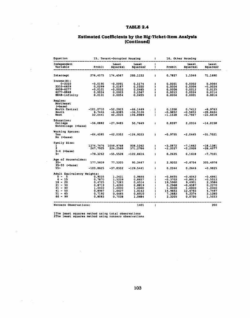
TABLE 2.4

Estimated Coefficients by the Big-Ticket-Item Analysis(Continued)

E q u a tio n 15 . T e nan t-O ccup ied H ousing I 16 . O th e r H ousing

In d e p e n d e n t Le a s t Le as t I L e a s t Le as tV a r ia b le P ro b it S q u a re s l Squares2 j P ro b it S q u a re s l Squares2

In te r c e p t 276.4075 174.4567 293.1152 1 0 .7857 1 .1 046 71.1690

In co m e ( $ ) :0 -3310 -0 .0 1 9 0 -0 .0 0 9 1 0 .1174 I 0 .0001 0 .0 002 0.0064

3310-4639 0.0299 0 .0187 0 .1550 I 0 .0004 0 .0 0 0 6 -0 .0 0 2 64639-6277 - 0.0101 -0 .0 0 3 2 0 .0465 I 0 .0006 0 .0 012 0.01256277-8848 0.0024 0 .0003 0.1567 I 0 .0013 0 .0024 0 .01148 8 4 8 - in f in i t y 0.0131 0 .0054 0 .0 455 I 0 .0004 0 .0001 0 .0 016

R e g io n :N o rth e a s t(•b a se )

N o r th C e n t ra l -1 0 1 .0 7 1 0 -5 2 .2 9 2 3 -6 6 .1 4 4 9 1 0 .1358 0 .7412 -8 .9 7 6 3S outh 6 .7446 -6 .6 3 8 5 -3 6 .5 1 2 6 1 -0 .9 8 5 2 -0 .5 8 5 3 -2 8 .8 6 3 4West 32.0441 40.2035 106.8989 1 -1 .1 5 3 8 -0 .7 9 4 7 -2 3 .6 4 1 8

E d u c a tio n :C o lle g e -3 6 .0 8 8 2 -2 7 .9 4 8 5 50.7649 1 0 .8397 2 .2 316 -1 4 .0 1 5 8N o n c o lle g e (-b a se )

W ork ing Spouse:Yes -6 4 .4 0 8 5 -4 2 .0 3 5 2 -1 2 4 .9 3 3 3 1 -0 .9 7 5 5 -2 .0 4 4 5 -3 1 .7 0 2 1No (°base)

F a m ily S iz e :1 1274.7476 1059.9768 908.1262 1 -3 .0 8 7 2 -7 .1 6 6 2 -1 8 .1 3 8 12 267.7925 224.2568 371.2786 1 -2 .2 0 2 7 -3 .2 9 2 8 -2 8 .4 0 7 73-4 (-b a se )5+ -7 9 .3 2 6 2 -5 5 .5 5 2 8 -1 2 2 .8 6 1 6 1 0 .2635 0.1618 -7 .7 1 0 1

Age o f H o u se h o ld e r:3 5 - 177.5639 77.5205 95.3447 1 2 .9202 -0 .6 7 5 4 305.497635 -55 (-b a se )55+ -1 0 3 .8 6 2 5 -3 7 .8 3 3 2 -129 .5 441 i 0 .2344 0 .2 646 -0 .9 8 2 5

A d u lt E q u iv a le n c y H e ig h ts : 0 - 5 0 .9005 1.2431 0 .9646 I -0 .8 4 5 5 -0 .6 0 4 2 -0 .6 8 6 16 - 1 5 0.7870 1 .5239 0 .8657 I -0 .3 7 0 2 -0 .8 9 1 3 -0 .5 5 1 2

16 - 20 0.4725 1.7283 0.6514 1 19 .5960 9.4901 2 .3 58621 - 30 0 .8719 1.4293 0 .8819 I 0 .2968 -0 .6 5 8 7 0 .227031 - 40 1.0000 1.0000 1.0000 I 1 .0000 1 .0 000 1 .000041 - 50 0.8987 1.0627 1.0142 1 14 .9653 12 .6793 4 .749751 - 65 0 .7192 0 .6685 0 .8910 I 7 .2682 5.2374 3 .1 28066 - 99 0 .8083 0.7038 1.0684 I 2 .3205 0 .0 730 1.5033

N onzero O b s e rv a tio n s : 1401 1 200

IT h e le a s t squ a res method u s in g t o t a l o b s e rv a t io n s 2The le a s t sq u a re s method u s in g nonzero o b s e rv a t io n s

103

TABLE 2.4

Estimated Coefficients by the Big-Ticket-Item Analysis(Continued)

E q u a tio n 18 . H o te ls and M o te ls I 19 . F u r n i tu r e

In d e p e n d e n t Le as t Le as t I L e a s t Le a s tV a r ia b le P ro b it S q u a re s l Squares2 1 P ro b it S q u a re s l Squares2

In te r c e p t -2 .6 4 7 8 -0 .6 3 8 3 26.7040 I - 10 .0210 -5 .6 1 5 3 49.4820

In co m e ($) :0-3310 0 .0023 0 .0027 0 .0001 I 0.0174 0.0178 0 .0245

3310-4639 0 .0126 0 .0112 0 .0181 I 0 .0360 0 .0351 0 .05174639-6277 0 .0109 0 .0112 0 .0 089 | 0 .0340 0 .0 340 0 .0 3396277-8848 0.0171 0.0190 0 .0184 I 0 .0298 0 .0 282 0 .03038 8 4 8 - in f in i t y 0 .0123 0.0128 0 .0 137 | 0 .0617 0 .0 6 5 0 0 .0828

R e g io n :N o rth e a s t(-b a se )N o rth C e n tra l -4 .8 5 4 9 -4 .7 1 7 0 -1 5 .7 6 3 2 | 14.9674 16 .1396 23.3364South -8 .6 6 8 4 -8 .4 0 2 7 -1 3 .2 5 8 0 I -7 .9 5 7 2 -4 .9 0 3 7 -1 1 .0 1 4 8N est -5 .9 4 4 6 -6 .7 3 0 3 -1 2 .6 9 0 3 1 17.1042 11.5383 23.0485

E d u c a tio n :C o lle g e 16.7510 15.3932 19 .7096 | -1 0 .3 2 5 0 -1 5 .8 6 7 0 -2 7 .1 4 8 1N o n c o lle g e (-b a se )

W ork ing Spouse:Yes 5.0128 4.6098 2.6972 I -0 .5 2 1 9 -1 .4 3 5 0 -1 .9 9 1 0No (-b a se )

F a m ily S iz e :1 -3 3 .0 5 4 4 24.6710 34.9920 | -1 8 2 .6 1 3 0 -1 3 6 .0 4 5 2 72.92652 3 .1191 6.8288 31 .8290 I -2 9 .9 4 9 2 -7 .2 5 7 4 14.56673 -4 (-b a se )5+ 3.9351 2.0087 -3 .1 7 4 8 I -8 .0 2 7 9 -7 .5 1 5 6 -3 5 .3 6 5 4

Age o f H o u se h o ld e r:3 5 - -3 .7 1 3 4 -3 .5 0 7 8 -5 .0 0 8 9 | 8 .3219 -4 .7 2 6 7 -1 5 .7 3 7 335 -55 (-b a se )55+ 0 .3280 0 .2767 4 .0308 I 0 .1339 1.1021 55.2370

A d u lt E q u iv a le n c y W e ig h ts :0 - 5 0 .4665 0.3721 0.4870 t 0 .9767 1 .3 926 1.00176 - 1 5 1.5135 1.5218 1 .3890 I 0 .8149 0 .8830 0.7793

16 - 20 0.5853 0.5893 0.5007 | 0 .0832 0 .0984 0.05772 1 - 3 0 0.6845 0.6533 0 .6 745 | 0 .7606 0 .7211 0 .738131 - 40 1.0000 1.0000 1 .0 000 | 1 .0000 1 .0 000 1.000041 - 50 1 .1837 1.1153 1 .0373 | 0 .1797 0 .1374 0.174451 - 65 1.1297 0.9978 1.0121 I 0 .3732 0 .3308 0.350866 - 99 1 .5432 1.3084 1 .4 496 | 0 .3690 0 .2648 0.3873

N onzero O b s e rv a tio n s : 2101 I 1B76

IT h e le a s t squ a res m ethod u s in g t o t a l o b s e rv a t io n s 2The le a s t squ a res method u s in g nonzero o b s e rv a t io n s

104

TABLE 2.4

Estimated Coefficients by the Big-Ticket-Item Analysis(Continued)

E q u a tio n 20. K itc h e n and H ousehold A p p lia I 21 . C hina , G lassw are ,, and Tab

Ind epe nde n t Le as t Le as t 1 L e a s t Le as tV a r ia b le P ro b it S qua res l Squares2 I P ro b it S q u a re s l Squares2

In te r c e p t -2 2 .6 5 9 2 -1 7 .9 6 6 0 2 .9993 I -1 5 .2 7 4 2 -1 0 .0 5 8 9 -5 .9 3 7 9

In co m e ($ ) :0-3310 0.0132 0 .0123 0.0121 I 0 .0048 0 .0 035 0 .0043

3310-4639 0.0104 0 .0112 0 .0087 I 0 .0065 0 .0 066 0 .01024639-6277 0.0091 0 .0065 0 .0082 I 0 .0077 0 .0 066 0 .00986277-8848 0.0128 0 .0127 0.0131 I 0 .0143 0 .0125 0 .01848 8 4 8 - in f in i t y 0.0045 0 .0043 0 .0055 I 0 .0024 0 .0023 0 .0 035

R e g io n :N o rth e a s t(•b a se )N o rth C e n t ra l 9.6081 10.1322 9 .0779 I 7 .3085 7 .2 466 9 .0723S outh 16.2805 17.1424 21.7212 I 2 .2494 3 .8402 4.8501West 9.5158 8.6291 7 .5148 1 32 .0259 28.3270 46.4714

E d u c a tio n :C o lle g e -4 .3 4 7 3 -3 .9 8 5 0 -6 .4 0 9 3 I 5 .8803 6.4763 1 .5068N o n c o lle g e (-b a se )

W ork ing Spouse:Yes 2.0205 2.5889 1.5183 I -6 .2 8 9 1 -5 .5 4 0 1 -1 2 .2 3 3 5No (-b a se )

F a m ily S iz e :1 -1 9 .3 4 3 9 -1 0 .3 0 2 4 59.4118 I -5 0 .6 9 2 3 -4 0 .7 8 5 4 -5 5 .1 6 8 02 -5 .3 9 5 0 -1 .7 7 5 2 13.8428 | -2 5 .4 2 0 3 -2 0 .8 8 0 1 -3 2 .7 0 7 13-4 ( “ base)5+ 0.2651 -1 .4 1 1 1 -1 2 .6 4 6 8 I 7 .9195 2.9921 8.3550

Age o f H o u se h o ld e r:3 5 - 10 .6675 9.9430 13.9710 I 9 .6106 5.6967 20.092335 -55 (-b a se )55+ -2 .1 3 0 4 -3 .5 0 7 2 1.1840 I 9 .0169 7.3107 18.5798

A d u lt E q u iv a le n c y W e ig h ts :0 - 5 0.8393 0 .7799 0 .8919 | -0 .4 9 2 5 -0 .4 3 2 2 -0 .5 3 4 26 - 1 5 0.8563 0 .8617 1 .0915 | -0 .2 5 9 2 -0 .2 4 9 0 -0 .2 4 3 8

16 - 20 0.7005 0 .6780 0 .8 219 I -0 .0 7 5 9 -0 .0 8 7 3 -0 .0 9 5 121 - 30 1.1158 1.0B36 1.1251 I 0 .9 879 1.0685 0.999331 - 40 1.0000 1.0000 1 .0000 I 1 .0000 1.0000 1 .000041 - 50 1.0704 1.0010 1.1214 1 0 .7185 0 .7 219 0.733451 - 65 1.2154 1.2040 1.1617 t 0 .4837 0.5073 0.486266 - 99 1.1106 1 .0270 1 .1179 I 0 .3673 0.2902 0.4067

N onzero O b s e rv a tio n s : 2410 1 1994

IT h e le a s t squ a res method u s in g t o t a l o b s e rv a t io n s 2The le a s t squ a res method u s in g nonzero o b s e rv a t io n s

105

TABLE 2.4

Estimated Coefficients by the Big-Ticket-Item Analysis(Continued)

E q u a tio n 22 . O th e r D u ra b le House F u rn is h i I 23 . F lo o r C o ve rin g s

Ind epe nde n tV a r ia b le P ro b it

Le as tS qua res l

Le as t | Squares2 j P r o b it

L e a s tS q u a re s l

Le a s tSquares2

In te r c e p t -2 6 .0 9 6 4 -2 2 .44 21 -5 .9 7 4 4 | -1 .5 5 2 9 -2 .0 0 1 8 3 .0 736

In co m e ( $ ) :0-3310 0 .0093 0 .0103 0 .0 086 | 0 .0005 0.0014 0 .0 016

3310-4 639 0.0137 0 .0138 0 .0 136 | 0 .0014 0 .0021 0.00614639-6277 0.0241 0 .0248 0 .0242 I 0 .0011 0 .0 0 1 9 0.00246277-8848 - 0 .0012 - 0.0011 -0 .0 0 3 4 I 0 .0 019 0 .0 035 0 .00628 8 4 8 - in f in i t y 0.0270 0 .0297 0 .0312 I 0 .0 049 0 .0 058 0 .0200

R eg io n :N o rth e a s t(“ base)N o rth C e n t ra l 16.8464 16.6858 14.8656 I 0 .7017 0 .9 132 -0 .1 9 9 4S outh 8 .7446 9.7691 9.2399 I 0 .5603 0 .1727 6.1776West 13 .5255 11.4073 9 .2397 | -0 .3 5 6 9 -2 .2 4 6 6 -1 .1 7 7 7

E d u c a tio n :C o lle g e 2 .6602 1 .4635 0 .2544 | 0 .2913 0 .5 186 4.6001N o n c o lle g e (-b a se )

W ork ing Spouse:Yes 9.6103 9.9264 14.2075 I 1.0187 1 .3 789 7 .9211No (-b a se )

F a m ily S iz e :1 -3 0 .9 6 2 1 -1 5 .3 2 8 7 59.6582 | 0 .0270 1 .9402 83.31152 0.4612 1 .6889 17.1852 I -0 .3 4 4 9 -0 .9 2 8 4 1.22133 -4 (-b a se )5+ 2.5954 -0 .2 7 1 6 -4 .6 9 1 1 I -0 .2 2 7 3 -0 .2 3 8 4 -1 0 .0 7 9 9

Age o f H o u se h o ld e r:3 5 - -1 .4 2 8 8 -6 .9 3 6 9 -9 .0 5 2 5 I 0 .5282 -1 .2 6 6 8 2 .394335 -55 (-b a se )55+ 0.0007 2.0234 13 .4386 | 2 .8997 3 .4 094 18 .5359

A d u lt E q u iv a le n c y W e ig h ts : 0 - 5 1 .3650 1 .4216 1 .4026 I 4 .8670 4.9868 2 .85556 - 1 5 0.3587 0.3754 0 .3871 | 5 .8279 1.7968 3 .3055

16 - 20 0.2433 - 0 .0222 0 .2 383 I 1 .2210 -0 .1 4 9 6 0.408121 - 30 0 .7239 0 .6623 0 .7 066 | 0 .4662 0.4042 0 .397331 - 40 1.0000 1 .0000 1 .0000 | 1 .0000 1 .0 000 1 .000041 - 50 0.9863 0 .8644 0 .9464 1 1 .8070 0.7523 1 .423751 - 65 0.6304 0 .5796 0 .6 056 I 0 .6499 0.5770 0 .490066 - 99 0.4604 0.3281 0 .4 456 | 1 .9422 0 .9 859 1 .6 969

N onzero O b s e rv a tio n s : 2626 I 739

IT h e le a s t sq u a re s method u s in g t o t a l o b s e rv a t io n s 2The le a s t squ a res method u s in g nonzero o b s e rv a t io n s

106

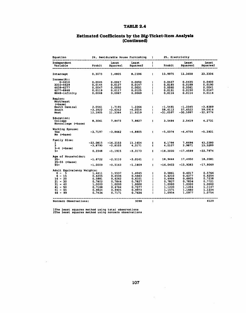
TABLE 2.4

Estimated Coefficients by the Big-Ticket-Xtem Analysis(Continued)

E q u a tio n 24 . S em idu rab le House F u rn is h in g | 25 . E l e c t r i c i t y

Ind epe nde n t Le as t Least 1 Le a s t Le as tV a r ia b le P ro b it S q u a re s l Squares2 I P ro b it S q u a re s l Squares2

In te r c e p t 0.3073 1.4805 8.1596 I 13 .9975 13.3658 33 .3306

In co m e ($) :0 -3310 0 .0045 0.0047 0.0050 I 0 .0437 0 .0 435 0 .0400

3310-4639 0.0144 0.0127 0.0147 1 0 .0185 0 .0188 0.01904639-6277 0 .0047 0.0050 0.0031 I 0 .0060 0 .0061 0.00416277-8848 0 .0 119 0.0117 0.0125 1 0.0151 0 .0 150 0 .01478 8 4 8 - in f in i t y 0 .0068 0 .0067 0 .0 069 I 0 .0116 0 .0114 0 .0 116

R e g io n :N o rth e a s t(•b a se )N o rth C e n t ra l 2 .0561 1 .7195 1 .2266 1 -1 .5 4 9 1 -1 .2 3 4 5 -3 .8 3 8 9S ou th -3 .3 9 2 2 -3 .6 3 4 2 -4 .0 0 1 4 1 58 .6112 57.6522 59 .0916West 12 .3905 11.3364 11.9219 I -3 1 .0 5 9 7 -3 0 .5 9 9 7 -3 2 .9 7 7 4

E d u c a tio n :C o lle g e 8.3061 7.8473 7 .9827 I 3 .5484 2 .5 4 1 9 4.2731N o n c o lle g e (°base)

W ork ing Spouse:Yes -3 .7 1 9 7 -3 .8 6 6 2 -4 .8 8 0 5 I -5 .0 3 7 4 -4 .4 7 5 6 -5 .3 9 3 1No (-b a se )

F a m ily S iz e :1 -2 2 .0 8 1 5 -1 6 .2 1 5 3 11.1654 1 6.1794 7 .8 696 43.23802 -3 .8 7 9 0 -2 .8 1 0 3 4.3171 I 4 .0107 3.9871 13.32893-4 (•base )5+ 0.2348 -1 .1 9 1 5 -3 .3 1 7 3 I -1 8 .2 0 0 0 -1 7 .4 5 9 9 -2 2 .7 9 7 4

Age o f H o u se h o ld e r:3 5 - -1 .6 7 2 2 -2 .5 1 1 0 -3 .0 1 4 1 f 18.9444 17.4950 18.358135-55 (»base)55+ -1 .0 0 0 9 -0 .5 1 6 3 -1 .1 8 0 9 I -1 6 .0 4 0 3 -1 5 .9 3 8 3 -1 7 .9 0 6 9

A d u lt E q u iv a le n c y W e ig h ts : 0 - 5 1 .4411 1 .5537 1.4045 I 0 .5861 0 .6 017 0 .5 7666 - 1 5 0.6205 0 .6536 0 .5663 I 0 .6210 0 .6 377 0 .6254

16 - 20 0.5881 0 .6262 0.6101 I 0 .6964 0 .6 805 0 .723821 - 30 0.7802 0 .7 846 0.7827 I 0 .7827 0 .7 836 0.772131 - 40 1 .0000 1 .0000 1 .0000 I 1 .0000 1.0000 1 .000041 - 50 0.7188 0.6764 0.7377 I 1 .1220 1.1204 1 .114751 - 65 0.9924 0 .9905 0 .9973 I 1.1571 1 .1 660 1.123466 - 99 0 .7436 0.7171 0.7636 1 1.0954 1 .0 977 1.0754

N onzero O b s e rv a tio n s : 3098 1 4129

IT h e le a s t squ a res method u s in g t o t a l o b s e rv a t io n s 2The le a s t squ a res method u s in g nonzero o b s e rv a t io n s

107

TABLE 2.4

Estimated Coefficients by the Big-Ticket-Item Analysis(Continued)

E q u a tio n 26 . N a tu ra l Gas I 27 . F ue l O i l and C oal

In d epe nde n t Le as t L e a s t | Le as t Le a s tV a r ia b le P ro b it S q u a re s l Squares2 j P ro b it S q u a re s l Squares2

I n te r c e p t 74 .2966 61.6927 124.1793 | 73 .6107 66.2490 72.5403

In co m e ($ ) :0-3310 0.0091 0 .0096 0.0123 I 0 .0082 0 .0127 0.0366

3310-4639 0 .0030 0 .0005 0.0020 | 0 .0030 -0 .0 0 0 9 -0 .0 0 2 84639-6277 0 .0156 0 .0 149 0 .0 1 4 9 | 0 .0 056 0 .0 060 0.03476277-8848 0.0013 0 .0015 0 .0 023 | 0 .0 086 0 .0 098 0.02058 8 4 8 - in f in i t y 0 .0052 0 .0042 0 .0 070 | 0 .0002 -0 .0 0 0 4 0.0071

R e g io n :N o rth e a s t(“ base)N o rth C e n t ra l 35 .4080 31.9321 -2 .4 7 9 1 | -1 0 0 .6 1 7 6 -1 0 3 .8 7 2 5 -8 5 .0 0 8 6S outh -4 5 .1 6 8 0 -3 8 .0 0 9 2 -6 5 .8 3 0 6 | -1 0 0 .0 1 1 5 -1 0 1 .5 3 9 2 -7 9 .1 0 2 6West -4 0 .1 8 7 4 -3 4 .6 1 7 8 -8 4 .0 8 2 9 | -1 14 .4 671 -1 1 9 .0 0 8 8 -1 4 5 .7 2 8 8

E d u c a tio n :C o lle g e 7.5575 6.8368 7.1863 | 5 .8307 7 .0 866 22 .5920N o n c o lle g e (-base )

W ork ing Spouse:Yes -7 .5 4 3 4 -4 .1 2 2 3 -6 .0 8 1 5 | 3 .7783 4 .9138 11.1641No (-b a se )

F a m ily S iz e :1 8.2370 16.5401 89 .9709 | 15 .0575 10.1523 283.95512 3.0862 7 .1765 30.8664 | 2 .6056 -0 .9 1 1 7 74 .37783-4 ("b a se )5+ -1 4 .4 8 8 6 -1 6 .4 7 1 1 -2 3 .3 8 6 9 | 7 .7368 9.8045 -1 8 .6 9 4 7

Age o f H o u se h o ld e r:3 5 - -0 .7 3 8 0 -1 .1 1 0 8 -4 .4 7 2 9 I -1 .3 0 4 6 -2 .0 3 2 4 -2 .6 7 1 935 -55 (-b a se )55+ 3.6063 3.0300 -0 .4 8 0 9 | 16 .6624 7 .0 618 33.7085

A d u lt E q u iv a le n c y W e ig h ts :0 - 5 0.7133 0.9304 0 .8308 I 0 .3793 -0 .1 4 6 5 0 .87026 - 1 5 0.6605 0 .8350 0 .7122 I 0 .9068 0 .2 516 1.0774

16 - 20 0 .6689 0.7939 . 0 .7285 I 1 .2420 1 .2221 1 .155721 - 30 0.7793 0 .8070 0 .8 459 | 0 .7199 0 .9 135 0 .888831 - 40 1 .0000 1.0000 1 .0000 I 1 .0000 1.0000 1 .000041 - 50 1 .1287 1.1974 1.1201 I 1 .1891 0 .9 617 1.156851 - 65 1 .0455 1.1442 1 .0 546 | 1 .3727 1 .3634 1 .2 17966 - 99 1.1421 1.2182 1 .1074 | 1 .5834 2 .2 069 1 .6474

N onzero O b s e rv a tio n s : 2894 | 658

IT h e le a s t sq u a res method u s in g t o t a l o b s e rv a t io n s 2The le a s t sq u a res method u s in g nonzero o b s e rv a t io n s

108

TABLE 2.4

Estimated Coefficients by the Big-Ticket-Item Analysis(Continued)

E q u a tio n 28 . Wood, O th e r F u e l, and B o t t le I 29 . W ater and O th e r S a n ita ry

In d e p e n d e n t Le as t Le as t I L e a s t Le as tV a r ia b le P r o b it S q u a re s l Squares2 I P r o b it S q u a re s l Squares2

In te r c e p t 4 .8007 7.6201 35.7122 I 2 .3966 1 .5648 25 .7446

Inco m e( $ ) :0 -3310 -0 .0 0 0 4 - 0 .0011 0 .0014 I 0 .0 086 0 .0 088 0 .0 059

3310-4639 0 .0000 0 .0002 -0 .0 1 4 9 I 0 .0022 0 .0024 0 .0 0154639-6277 0 .0007 0 .0004 0.0090 I 0 .0027 0 .0 025 0 .0 0096277-8848 -0 .0 0 0 4 - 0 .0002 -0 .0 0 7 4 1 0 .0043 0 .0 040 0 .0 0568 8 4 8 - in f in i t y 0 .0007 0 .0 009 0 .0 029 I 0 .0013 0 .0 013 0.0007

R eg io n :N o rth e a s t(•base )N o rth C e n t ra l 0 .3103 0.6254 9 .3016 1 8 .0682 7 .7 889 3 .0 226South 0 .6 4 90 1.1067 8.7361 I 19.9011 19.3945 17.9207West -2 .1 0 2 4 -2 .5 4 3 2 -7 .5 8 4 5 1 14 .7122 13.8261 12 .8666

E d u c a tio n :C o lle g e -0 .1 3 7 1 -0 .7 2 6 8 -0 .2 1 1 9 I 2 .4328 2 .6 449 0 .9 399N o n c o lle g e (-b a se )

W ork ing Spouse:Yes 1.4426 1 .4039 7.2172 I 2 .8378 3 .0 6 0 9 1.4001No (-b a se )

F a m ily S iz e :1 10.6899 8.6932 151.1930 I 2 .3 649 0 .9 826 53.61412 3 .8835 2.4363 37.6814 1 0 .9410 -0 .2 1 3 3 13.50633 -4 (-b a se )5+ -1 .2 2 2 6 -1 .6 6 4 8 -1 0 .5 3 4 2 1 -3 .5 1 1 0 -3 .7 2 8 2 -9 .7 8 3 4

Age o f H o u se h o ld e r:3 5 - -0 .6 2 8 0 -1 .1 5 1 0 -5 .4 9 6 0 1 -2 .7 1 3 8 -1 .5 3 5 9 -0 .7 8 8 335 -55 (-b a se )55+ -0 .3 6 9 4 -0 .7 7 3 4 -3 .3 8 7 0 I 1 .5088 0.2175 -4 .1 7 3 9

A d u lt E q u iv a le n c y W e ig h ts : 0 - 5 2 .3627 1 .6259 2 .2065 I 0 .8116 0 .7 883 0 .7 1766 - 1 5 0.6417 0.6022 0 .7608 I 0 .8043 0.8098 0 .8158

16 - 20 1.7439 1.5951 1 .7420 1 0 .5718 0 .5 633 0 .679721 - 30 0.7777 0.6885 1 .1196 I 0 .8 936 0 .8 360 0 .991131 - 40 1.0000 1 .0000 1 .0000 I 1 .0000 1 .0000 1 .000041 - 50 1.6601 1 .3320 1 .1628 I 1 .1038 1 .1 099 1 .067151 - 65 2.3184 2.3707 1 .8179 i 1 .0985 1 .1431 1 .0 44966 - 99 1.9911 1 .7737 1 .7892 I 1 .0817 1 .2082 1 .0560

N onzero O b s e rv a tio n s : 482 1 3160

IT h e le a s t sq u a res method u s in g t o t a l o b s e rv a t io n s 2The le a s t squ a res method u s in g nonzero o b s e rv a t io n s

109

TABLE 2.4

Estimated Coefficients by the Big-Ticket-Item Analysis(Continued)

E q u a tio n 30 . Te lephone and T e le g ra p h I 31 . D om e stic S e rv ic e s

Ind epe nde n tV a r ia b le P ro b it

Le as t S q u a re s l

L e a s tSquares2

1I P ro b it

L e a s tS q u a re s l

L e a s tSquares2

In te r c e p t 64.2882 63.2736 68.6554 I -4 .2 6 6 1 -2 .5 8 9 4 4 .7 036

In co m e ($ ) :0 -3310 0.0182 0 .0187 0 .0170 | 0 .0062 0 .0 016 0 .0122

3310-4639 0.0073 0.0071 0 .0075 I 0 .0124 0.0050 0 .02674639-6277 0.0104 0.0104 0 .0100 I 0 .0105 0.0057 0 .01766277-8848 0.0120 0.0121 0 .0117 I 0.0021 0 .0 002 0 .00688 8 4 8 - in f in i t y 0.0134 0.0134 0 .0133 I 0 .0 125 0 .0 127 0 .0 219

R eg io n :N o rth e a s t(•base )N o rth C e n t ra l -7 .0 7 4 0 -7 .14B B -6 .9 9 3 2 I -2 .6 2 2 9 -0 .7 1 0 0 -6 .8 0 7 3South 0 .8520 0.587B 1.5684 I 13.766B 2 .9881 33 .0125West -1 1 .5 9 5 0 -1 1 .5 8 3 3 -1 1 .6 6 3 3 I -3 .9 7 9 6 -1 .1 6 0 4 -6 .9 8 4 8

E d u c a tio n :C o lle g e 11.9851 11.9764 11.7507 1 -2 .0 9 1 3 1 .4072 -1 2 .8 7 0 5N o n c o lle g e <=base)

W ork ing Spouse:Yes -1 3 .0 3 2 9 -1 2 .6 9 1 3 -1 3 .5 0 9 0 I 8 .9548 4 .6538 13.0614No (-b a se )

F a m ily S iz e :1 88.1180 88.6047 96.8380 I -5 6 .3 1 5 7 -1 7 .0 4 4 7 -1 3 6 .9 3 2 02 25.0518 25.0468 26.1204 I -4 5 .4 9 2 2 -9 .3 0 3 5 -1 1 6 .0 4 3 73 -4 <=base)5+ -1 8 .1 0 0 1 -1 7 .9 0 4 7 -1 9 .1 0 2 1 I -1 1 .4 5 3 3 -3 .3 0 7 4 -2 7 .1 5 4 1

Age o f H o u se h o ld e r:3 5 - 5 .4000 5.1961 5.4273 I 4 .2870 1.5032 7.010135 -55 («base) 55+ -1 4 .5 9 0 6 -1 4 .7 2 5 4 -1 4 .5 3 0 3 I 5 .6877 0.4905 25 .1970

A d u lt E q u iv a le n c y W e ig h ts : 0 - 5 0 .4742 0.4752 0.4829 I 9 .2928 32 .2522 5 .17006 - 1 5 0.4912 0.4883 0 .4980 1 2 .1176 4.7494 1.5948

16 - 20 0 .9757 0.9684 0 .9 939 I 1 .3481 2.9292 1.72342 1 - 3 0 1.0052 1.0035 1.0013 I 0 .8750 0 .4 177 1 .1 76631 - 40 1 .0000 1.0000 1 .0000 I 1 .0000 1.0000 1 .000041 - 50 1 .0077 1.0053 1 .0055 1 1.1641 1.7057 1.512151 - 65 0 .8736 0 .8710 0.8804 I 1 .1921 0.9217 0 .9 81966 - 99 0 .7868 0 .7809 0 .7910 I 8 .0074 10.9734 8 .1948

N onzero O b s e rv a tio n s : 4321 I 1155

IT h e le a s t squ a res method u s in g t o t a l o b s e rv a t io n s 2The le a s t squ a res method u s in g nonze ro o b s e rv a t io n s

110

TABLE 2.4

Estimated Coefficients by the Big-Ticket-Item Analysis(Continued)

E q u a tio n 32 . O th e r H ousehold O p e ra tio n s I 33 . H ousehold In s u ra n c e

Ind epe nde n tV a r ia b le P ro b it

Le as tS qua res l

Le as tSquares2

1I P ro b it

Le a s tS q u a re s l

Le as tSquares2

In te r c e p t -1 0 .9 2 6 2 -8 .1 7 2 0 2.5948 I -9 .5 1 9 6 -8 .7 6 5 6 43 .1899

In co m e ($ ) :0 -3310 0.0039 0.0039 0 .0038 I 0 .0092 0.0102 0 .0042

3310-4639 0.0223 0.0194 0 .0278 I 0 .0055 0.0062 0 .00654639-6277 0.0064 0 .0066 0.0049 I 0 .0053 0 .0 062 0 .00386277-8848 0.0157 0.0162 0.0210 I 0 .0 079 0 .0 085 0 .00708 8 4 8 - in f in i t y 0.0458 0.0479 0 .0502 I 0 .0034 0.0034 0 .0 049

R e g io n :N o rth e a s t(-b a se )N o rth C e n t ra l 18 .6342 16.0784 21.9643 I 5 .5789 5 .8808 -1 .8 1 4 3South 11 .0996 9 .1127 14.4186 1 1.4301 0 .6 795 3.1311West 23 .4372 19.3384 26.8982 I -3 .8 0 5 3 -4 .4 3 5 8 -3 .6 9 0 1

E d u c a tio n :C o lle g e 20.4622 18.7007 20.6319 I 9 .6734 9 .1542 5.4105N o n c o lle g e (-b a se )

W ork ing Spouse:Yes -1 1 .7 0 3 8 -9 .7 5 8 0 -1 8 .3 0 5 9 I 1 .0449 3 .2 737 -2 .4 3 6 7No (-b a se )

F a m ily S iz e :1 -7 .0 7 1 9 8.4321 37.1383 I -7 .7 0 2 6 -0 .7 8 5 0 55.46542 -1 8 .0 1 7 3 -1 4 .0 6 7 9 -1 3 .1 8 1 3 I -1 .5 2 0 6 -0 .2 8 9 5 9.26553 -4 (-b a se )5+ 4.5856 3 .4 005 1 .5579 I -0 .2 4 3 6 -0 .2 4 6 2 -1 2 .8 9 2 2

Age o f H o u se h o ld e r:3 5 - -2 .4 9 5 7 -4 .0 2 6 8 -3 .1 7 2 2 I 0 .4188 3.9988 2.951935 -55 (-b a se )55+ -0 .9 4 9 4 -0 .8 3 3 3 -9 .5 1 9 5 I 9 .7095 5 .7 489 3.6737

A d u lt E q u iv a le n c y W e ig h ts : 0 - 5 1 .4714 1.6804 1.4280 I 0 .6967 0 .664 5 0.66576 - 1 5 0.8541 0 .8795 0 .7130 I 0 .6816 0 .4 889 0.6680

1 6 - 2 0 0.0757 0 .0787 0 .0796 I 0 .3116 0 .0 4 1 6 0.314221 - 30 0 .3985 0 .2835 0 .4293 I 0 .9450 0.6290 0.878231 - 40 1 .0000 1 .0000 1 .0000 I 1 .0000 1.0000 1 .000041 - 50 0 .4662 0 .4272 0.4433 I 1 .1564 1 .0 406 1 .098851 - 65 1 .1921 1 .1776 1.1241 1 1 .1579 1.0730 1 .106966 - 99 1 .1256 1.0311 1.0230 I 1 .2962 1 .3387 1 .2143

N onzero O b s e rv a tio n s : 2973 1 2224

IT h e le a s t squ a res method u s in g t o t a l o b s e rv a t io n s2The le a s t squ a res method u s in g nonzero o b s e rv a t io n s

TABLE 2.4

Estimated Coefficients by the Big-Ticket-Item Analysis(Continued)

E q u a tio n 34 . P r e s c r ip t io n Drug and S u n d rl I 35 . P h y s ic ia n s

Ind epe nde n tV a r ia b le P ro b it

LeastS q u a re s l

Le a s tSquares2

1j P r o b it

L e a s tS q u a re s l

Le a s tSquares2

In te r c e p t -6 .0 8 0 3 -5 .6 3 0 2 2 .7040 I -3 .7 4 5 4 -4 .3 1 9 2 12.7249

In co m e ($) :0-3310 0 .0055 0 .0056 0 .0042 I 0 .0135 0 .0 133 0 .0123

3310-4639 0 .0055 0 .0055 0 .0068 I 0 .0151 0 .0144 0 .01394639-6277 0.0024 0 .0022 0 .0 019 I 0 .0 099 0 .0084 0 .00936277-8848 0 .0016 0 .0023 0 .0020 I 0 .0010 0 .0 0 1 9 0 .00128 8 4 8 - in f in i t y 0 .0016 0 .0013 0 .0 019 I 0 .0142 0 .0 143 0 .0155

R e g io n :N o rth e a s t(•b a se )N o rth C e n t ra l 5 .3047 6.0196 5 .2319 1 -3 .6 0 2 1 -3 .6 6 5 9 -3 .6 3 5 5South 9.5362 10.1365 10.2420 I 4 .2528 2 .0242 7.2128West -0 .4 1 9 2 -0 .4 8 7 3 0 .9 009 I -3 .7 2 2 3 -3 .7 3 4 4 4.2633

E d u c a tio n :C o lle g e -2 .9 7 7 2 -3 .4 1 4 1 -3 .9 9 5 3 1 6.2254 3 .1 648 9.7638N o n c o lle g e (-b a se )

W ork ing Spouse:Yes -0 .9 8 2 0 -0 .9 3 6 1 -2 .3 0 6 0 1 -1 2 .5 7 6 3 -1 0 .3 3 7 5 -1 8 .7 1 8 1No (-b a se )

F a m ily S iz e :1 -6 .8 2 9 2 -5 .8 6 8 9 2.8809 I -3 1 .3 4 6 0 -2 3 .5 2 6 4 9.69222 -1 .7 1 5 0 -1 .5 8 2 3 1 .2625 I 7 .9643 9.0244 23.51133-4 (-b a se ) 5+ -0 .4 7 4 3 -0 .2 7 1 3 -2 .4 7 1 1 1 1 .4393 -1 .0 0 7 6 -2 .0 6 3 6

Age o f H o u se h o ld e r:35 - -0 .6 8 4 4 0.0667 -0 .4 7 9 6 1 -0 .7 1 5 2 1 .2 349 -2 .7 5 3 335 -55 (-b a se )55+ 4.6330 3 .7498 3.8022 1 9 .9095 9.8597 6.9458

A d u lt E q u iv a le n c y W e ig h ts : 0 - 5 0 .8537 0.7687 0.6638 1 1 .0885 1.5257 1.24206 - 1 5 0.5941 0 .5099 0.6127 1 0 .4066 0.4081 0.4111

16 - 20 1.0100 0.8687 1.0571 1 1 .3015 1.5280 1.340121 - 30 0 .8396 0.7592 0 .8535 I 0 .7674 0 .7124 0.828531 - 40 1.0000 1.0000 1 .0000 I 1 .0000 1 .0 000 1.000041 - 50 1.8186 1.8278 1 .7573 I 0 .9261 0 .8 960 0.928451 - 65 2.2630 2.1533 2 .2210 I 0 .7172 0.7060 0.747566 - 99 4.3908 4 .4220 3 .6583 I 1 .4214 1.4414 1.2826

N onzero O b s e rv a tio n s : 3384 | 32S2

IT h e le a s t sq u a res method u s in g t o t a l o b s e rv a t io n s 2The le a s t sq u a res method u s in g nonzero o b s e rv a t io n s

112

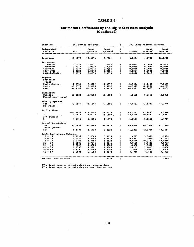
TABLE 2.4

Estimated Coefficients by the Big-Ticket-Item Analysis(Continued)

E q u a tio n 36 . D e n ta l and Eyes 1 37 . O th e r M e d ic a l S e rv ic e s

In d epe nde n t Le as t Le a s t 1 Le a s t Le as tV a r ia b le P ro b it S q u a re s l Squares2 I P ro b it S q u a re s l Squares2

In te r c e p t -1 5 .1 2 7 2 10.6795 -2 .2 0 0 1 t 6 .0034 4 .0 706 23.2295

In co m e ( $ ) :0 -3310 0.0134 0 .0121 0 .0150 1 0 .0010 0 .0 006 0 .0000

3310-4639 0.0114 0 .0108 0.0095 1 0 .0045 0 .0023 0 .0 0864639-6277 0 .0077 0 .0076 0.0055 I 0 .0 036 0 .0023 0 .00466277-8848 0.0082 0 .0078 0.0081 I 0 .0014 0 .0 006 0 .00308 8 4 8 - in f in i t y 0.0074 0 .0075 0.0073 I 0 .0028 0 .0 019 0 .0042

R e g io n :N o rth e a s t(-b a se )N o rth C e n t ra l -2 .5 5 5 5 -2 .6 7 0 2 -4 .8 9 7 7 1 -3 .5 9 9 4 -2 .1 4 0 0 -7 .1 5 8 9S outh -0 .0 5 7 4 0 .5108 1.9997 1 -0 .3 9 7 3 -0 .4 2 0 6 0 .4 289West -1 .7 0 0 7 -1 .3 4 1 9 2.0474 t -0 .9 5 3 2 -0 .5 6 6 5 -1 .8 4 0 2

E d u c a tio n :C o lle g e 18.8224 18.0592 18.1980 I 1 .8600 0 .2 595 2.8875N o n c o lle g e (=base)

W ork ing Spouse:Yes -2 .9 8 5 9 -3 .1 3 4 5 -7 .1 6 8 6 1 -3 .0 6 8 3 -1 .1 2 8 3 -6 .2 0 7 8No (-b a se )

F a m ily S iz e : 1 -1 3 .7 4 7 9 11.3700 18.0577 1 -5 .1 7 1 3 -2 .8 4 9 7 8.59162 0 .9616 1.0033 16 .1597 . I -2 .4 7 4 9 -0 .5 8 8 2 -1 .4 0 3 23 -4 (-b a se )5+ 4 .9418 3 .4396 1 .1778 1 -1 .3 1 3 6 -1 .6 1 1 8 -5 .7 7 4 7

Age o f H o u se h o ld e r:3 5 - -3 .5 6 5 7 -4 .7 1 8 8 -1 .6 8 7 5 1 -0 .0 3 4 8 -0 .7 5 6 4 -1 .1 5 1 835 -55 (“ base)55+ -6 .4 7 9 4 -6 .6 4 3 9 -9 .4 2 3 0 I -1 .2 2 3 3 -2 .0 7 1 6 -8 .1 6 1 4

A d u lt E q u iv a le n c y W e ig h ts : 0 - 5 0 .4137 0 .4503 0.4114 1 1 .4777 3 .0 029 1 .28966 - 1 5 1 .5026 1 .5748 1.3474 I 0 .8537 2 .0 089 0 .7735

16 - 20 1.2706 1.3495 1.2824 I 0 .0340 -0 .0 1 6 2 -0 .0 6 1 621 - 30 0.7501 0 .7076 0.8041 I 0 .9128 1 .4 442 0 .8 73931 - 40 1.0000 1 .0000 1.0000 1 1 .0000 1 .0 000 1 .000041 - 50 1.4795 1.4701 1 .4749 1 2.0161 2 .6 013 1 .906851 - 65 1.8290 1 .8589 1.7053 I 1 .7076 2 .4677 1 .630866 - 99 2.0694 2 .1090 1.8173 1 3 .7946 7 .7 549 3.7362

N onzero O b s e rv a tio n s ; 3033 1 1819

IT h e le a s t squ a res method u s in g t o t a l o b s e rv a t io n s2The le a s t squ a res method u s in g nonzero o b s e rv a t io n s

TABLE 2.4

Estimated Coefficients by the Big-Ticket-Item Analysis(Continued)

E q u a tio n 38 . H o s p ita ls and S a n ita r iu m s 11 39 . H e a lth In s u ra n c e

Ind epe nde n t Least Le a s t 11 L e a s t L e a s tV a r ia b le P ro b it S q u a re s l Squares2 I P r o b it S q u a re s l Squares2

In te r c e p t -0 .8 5 1 4 -1 .2 9 9 2 15.7134 I -4 .8 5 9 2 -1 4 .3 8 6 8 32.3418

In co m e (5 ) :0-3310 0.0011 0.0011 0.0064 I 0 .0140 0 .0 152 0 .0157

3310-4639 0.0018 0 .0017 0 .0 090 II 0 .0 199 0 .0 207 0.02974639-6277 0.0030 0 .0 019 0 .0167 |1 0 .0057 0 .0 063 0 .00606277-8848 -0 .0 0 5 3 -0 .0 0 4 5 -0 .0 2 2 4 II 0 .0038 0 .0 025 0 .01058 8 4 8 - in f in i t y 0.0077 0 .0095 0 .0264 |I 0 .0027 0 .0 027 0 .0038

R e g io n :N o rth e a s t(-b a se )N o rth C e n t ra l 0 .1147 0.1214 -9 .5 2 7 1 1 15 .5410 14.3642 23 .8358S outh 2.3871 1.9394 2 .1228 1 20 .9693 24.1743 17.7064West 0.3207 0.7004 -6 .6 4 3 5 1 9.4555 8 .3 058 12 .5525

E d u c a tio n :C o lle g e -0 .6 2 3 1 -1 .7 2 5 0 -2 .8 5 1 4 1 -4 .2 0 5 8 -1 .3 6 3 2 -9 .0 1 8 1N o n c o lle g e (-b a se )

W ork ing Spouse:Yes -1 .8 0 0 3 -0 .3 0 4 3 -1 0 .0 3 3 5 1 -7 .9 2 1 9 -4 .5 8 8 9 -1 5 .9 3 9 2No (-b a se )

F a m ily S iz e :1 7.2801 5.8649 254.6240 1 11.1624 6 .2384 45.15332 4.3461 6.6017 51.7363 1 16 .1595 11 .8222 40.51973 -4 (-b a se )5+ -0 .0 3 6 9 -0 .8 4 7 8 -8 .2 7 6 2 1 -8 .8 2 4 4 -5 .3 1 4 8 -2 5 .0 9 3 6

Age o f H o u se h o ld e r:3 5 - 1.2908 -0 .1 8 3 0 2 .4232 1 5.4459 9 .4 806 13.361735-55 (-b a se )55+ 1.8460 1.3256 2.7674 1 19 .8882 18.9322 8 .1026

A d u lt E q u iv a le n c y W e ig h ts : 0 - 5 2 .4946 0.5754 0.9694 1 0 .8325 0.6358 0.74346 - 1 5 3.4781 4.5840 2.0847 1 0 .5024 0.3674 0 .5 813

16 - 20 10.2838 8.8355 4.0998 1 0 .8785 0 .6784 1.073221 - 30 1 .2659 0.5364 1.0550 1 0.7584 0 .7 828 0.789131 - 40 1 .0000 1 .0000 1.0000 I 1 .0000 1 .0 000 1.000041 - 50 1.5664 1 .4513 0.8974 I 1 .2712 1 .3 726 1 .1 21951 - 65 2.1717 0 .4 990 1.2777 1 1.4571 1 .5 466 1.221766 - 99 2.0042 1 .8158 1.1153 1 1 .9976 2 .2580 1 .2568

N onzero O b s e rv a tio n s : 853 1 2834

IT h e le a s t squ a res method u s in g t o t a l o b s e rv a t io n s 2The le a s t squ a res m ethod u s in g nonzero o b s e rv a t io n s

114

TABLE 2.4

Estimated Coefficients by the Big-Ticket-Item Analysis(Continued)

E q u a tio n 40 . P e rso n a l B us iness | 41 . L i f e In s u ra n c e

In d epe nde n tV a r ia b le P ro b it

Le as tS q u a re s l

L eastSquares2

1j P ro b it

Le a s tS q u a re s l

L e a s tS qua res l

In t e r c e p t -2 6 .3 2 4 7 -2 6 .1 5 8 4 6.6585 1 -4 3 .2 1 5 0 -4 1 .3 5 0 3 8.0188

In c o m e (S ):0-3310 0.0164 0.0161 0 .0 106 1 0 .0363 0 .0 362 0.0298

3310-4639 0 .0200 0.0190 0 .0 209 I 0 .0188 0 .0 215 0 .0 1864639-6277 0 .0 169 0 .0 169 0.0150 I 0 .0145 0 .0 119 0 .0 1166277-8848 0.0198 0.0193 0.0182 I 0 .0351 0 .0 367 0.03658 8 4 8 - in f in i t y 0 .0139 0.0137 0.0138 I 0 .0230 0 .0 2 0 6 0.0244

R eg io n :N o rth e a s t(-b a se )

N o rth C e n t ra l 12.4794 13.1181 6.8850 I 8 .4692 10 .0195 6 .7978S outh 15.3226 16.7056 11.6525 I 29 .8888 30.5601 27 .3707West 9.1963 9.9664 3.7113 I -6 .5 0 3 4 -4 .1 2 0 5 9.2914

E d u c a tio n :C o lle g e -5 .8 7 3 8 -6 .0 3 5 3 -9 .1 0 5 9 1 28 .5561 29 .9093 25 .1947N o n c o lle g e (-b a se )

W ork ing Spouse:Yes 0.0351 1 .4176 -6 .0 4 3 3 1 15 .6284 17.8114 11.2941No (-b a se )

F a m ily S iz e :1 -5 2 .6 4 0 4 -4 1 .1 1 8 7 -2 7 .2 9 3 9 1 -1 3 4 .5 0 1 1 -1 0 5 .4 8 7 9 -1 1 .1 5 2 62 -1 5 .1 3 3 4 -1 3 .6 5 0 8 -6 .3 0 4 4 1 -3 7 .3 3 2 4 -3 0 .6 3 0 7 -1 2 .9 1 2 73 -4 (-b a se ) 5+ 11.9995 10.3704 8.0386 1 -0 .6 5 4 6 0 .3 060 -1 2 .9 2 3 1

Age o f H o u se h o ld e r:3 5 - 16.7332 15.0983 16.7798 1 0.4861 1.8484 5.207535-55 (-b a se )55 + 8.9446 9.1027 13.2371 I 11 .6977 13 .4896 4.6153

A d u lt E q u iv a le n c y W e ig h ts :0 - 5- 0 .4470 0.4892 0 .4 596 1 0 .8437 0 .8091 0 .82426 - 1 5 0.1864 0.2092 0.2183 1 0 .4176 0.3450 0 .4747

16 - 20 0.1792 0.1733 0.2353 1 0 .6486 0.5630 0 .765321 - 30 0.6992 0.7074 0 .7096 I 0 .5406 0.4972 0 .579331 - 40 1.0000 1 .0000 1 .0000 I 1 .0000 1.0000 1 .000041 - 50 1.0160 0.9874 1 .0395 1 0 .9478 0 .9 375 0 .9 45651 - 65 1 .1009 1 .1097 1.1062 1 1 .0946 1 .0 680 1 .118566 - 99 1.1134 1.0814 1 .1016 I 0 .4818 0 .4031 0.6067

N onzero O b s e rv a tio n s : 3537 | 2882

IT h e le a s t sq u a re s method u s in g t o t a l o b s e rv a t io n s 2The le a s t sq u a res method u s in g nonzero o b s e rv a t io n s

115

TABLE 2.4

Estimated Coefficients by the Big-Ticket-Item Analysis(Continued)

E q u a tio n

In d e p e n d e n tV a r ia b le

42 . New

P ro b lt

Cars

Le as tS qua res l

Le as tSquares2

1 43 . Used

t1 P ro b lt

C ars

L e a s tS q u a re s l

Le a s tSquares2

In te r c e p t

In co m e {$) :

110.1007 -6 5 .0 5 1 9 814.9602 I -3 0 8 .3 1 7 6 -2 4 7 .5 7 2 7 -2 9 5 .2 9 2 0

0-3310 0 .0195 0.0244 0.2562 I 0 .0858 0 .0874 0 .1 9893310-4639 0 .0776 0.1006 0.5895 I 0 .0738 0 .0 592 0.20224639-6277 0 .1079 0.1466 0.2535 1 0 .0 746 0 .0 823 0 .2 1866277-8848 0 .1782 0.1984 0.3900 I 0 .0543 0 .0 306 O.180O8 8 4 6 - in f in i t y

R e g io n :N o rth e a s t(-b a se )

0 .1138 0.1225 0.1743 1 0 .0 446 0 .0 290 0.1475

N o rth C e n t ra l 35 .6797 30.1251 505.9614 1 120.2847 117.1247 258.0220S outh -9 .9 6 0 2 -6 .6 5 5 1 502.9802 1 88 .9815 62.8541 246.5538West -1 8 .7 1 1 7 -4 6 .3 4 0 9 466.1824 1 84 .6340 86 .6313 217.6908

E d u c a tio n :C o lle g eN o n c o lle g e (-b a se )

-6 2 .5 4 6 8 -4 9 .2 7 3 6 -5 6 8 .5 7 3 0 I -7 8 .1 4 4 9 -7 4 .0 6 8 0 41.4491

W ork ing Spouse:YesNo (-b a se )

F a m ily S iz e :

-2 7 .2 7 9 9 -3 7 .2 3 9 6 -4 7 5 .9 8 6 6 I 28 .1630 16.6172 -2 9 .8 6 4 3

1 •543.0374 -5 8 4 .1 1 6 5 2533.0942 I -9 7 .2 6 2 8 -6 9 .2 7 6 6 1147.163323 -4 (-b a se )

-230.6186 -2 4 1 .6 3 1 0 399.5923 I -7 6 .6 7 0 4 -7 5 .1 8 1 3 400.8611

5+ 107.8634 77.3945 53.1620 I 129.7850 120.5218 87 .8452

Age o f H o u se h o ld e r:3 5 -35-S5 (-b a se )

64.2933 38.6084 541.1436 I 9 .0267 -7 .0 7 7 3 64.4651

55+ 39 .9267

A d u lt E q u iv a le n c y W e ig h ts :

3 .3022 -4 38 .8 684 I 37 .6257 34 .0295 66.7103

0 - 5 1 .7656 1.1331 0.3987 1 0 .7223 0.2265 0.55726 - 1 5 1.4714 0 .6116 0 .3175 1 0 .7956 0 .2 925 0 .5 626

16 - 20 1.7064 1 .0088 0 .4720 1 0 .9973 1.0791 0 .4 1692 1 - 3 0 1.2577 1 .2199 0 .9176 I 1 .1461 1.4427 0 .868031 - 40 1.0000 1 .0000 1 .0000 I 1 .0000 1 .0 000 1 .000041 - 50 1.2101 0 .7121 0 .9232 I 0 .7999 0 .7504 0 .725151 - 65 1.1491 0 .8646 0 .9154 I 0 .7251 0 .5732 0 .822066 - 99 1 .8959 0 .8252 0 .9847 I 0 .4297 0 .3671 0 .7527

N onzero O b s e rv a tio n s : 313 1 690

IT h e le a s t squ a res method u s in g t o t a l o b s e rv a t io n s 2The le a s t squ a res method u s in g nonzero o b s e rv a t io n s

116

TABLE 2.4

Estimated Coefficients by the Big-Ticket-Item Analysis(Continued)

E q u a tio n

Ind epe nde n tV a r ia b le

44. New

P ro b it

and Used T ru cks o r Vans |

Le a s t L e a s t | S q u a re s l Squares2 I

1 45 . T ir e s

1I P ro b it

and Tubes

L e a s tS q u a re s l

L e a s tSquares^

In te r c e p t -7 6 .4 9 7 0 -9 4 .5 4 3 6 -2 0 4 .0 6 4 5 |I -4 1 .2 2 0 0 -3 5 .30 09 -1 8 .4 7 4 1

In co m e ( $ ) :0-3310 0 .0146 0 .0224 0 .1 500 |I 0 .0188 0 .0 189 0 .0 175

3310-4639 0 .0195 0 .0378 0 .1 226 |I 0 .0115 0 .0 119 0 .0 1134639-6277 0 .0430 0 .0745 0 .3714 |I 0 .0081 0 .0077 0 .0 0566277-8848 0 .0313 0 .0384 0 .1 687 |I 0 .0081 0 .0078 0.00818 8 4 8 - in f in i t y 0 .0127 0 .0114 0 .1 405 |I 0 .0029 0 .0028 0 .0 026

R eg io n :N o rth e a s t(-b a se )N o rth C e n t ra l 18.0351 30 .2619 102.9469 |1 3 .1601 2 .3 039 5 .2388S outh 25.3204 37.5888 59.9460 |1 13.7651 14 .3558 12.0040N est 41.6011 71.5741 60.3368 |1 20 .4164 21.2464 20.9370

E d u c a tio n :C o lle g e -3 1 .9 7 8 0 -6 8 .6 7 9 3 34.0851 11 -4 .8 0 9 5 -4 .4 3 0 0 -4 .8 4 2 6N o n c o lle g e (-b a se )

W ork ing Spouse:Yes 5 .9912 13.3914 23.5457 11 5 .3608 3 .6 9 9 6 2.9260No (-b a se )

F a m ily S iz e :1 -3 9 .3 6 5 4 -6 6 .8 4 6 1 2250.6279 |1 -1 4 .3 9 5 1 -4 .2 2 2 5 68.02602 -4 3 .2 1 3 4 -8 6 .7 1 0 7 -1 .7 7 7 4 I1 0 .4613 2 .9 886 20.09393 -4 (-b a se )5+ 32.9735 44.0080 -2 6 .3 2 0 2 |1 12 .1167 9.4962 1 .5 236

Age o f H o u se h o ld e r:3 5 - 15 .5352 18.0062 -4 1 .4 7 6 6 I1 7 .0371 2.9278 4 .179535 -55 (-b a se )55+ 6.7527 5 .7687 -1 2 6 .7 6 2 6 |1 -2 .2 7 9 6 0.9354 5 .2910

A d u lt E q u iv a le n c y W e ig h ts : 0 - 5 3 .1896 2 .8183 2 .2334 I1 0 .2958 0 .2 346 0 .4 2696 - 1 5 2.5555 0 .4957 1.6531 |1 0 .5052 0 .4661 0 .6453

16 - 20 1.4236 0.0224 0 .9215 I1 0 .9967 0 .9 049 1 .059321 - 30 1.1864 0 .7328 0 .9562 |1 1 .0642 1 .0 553 1 .0 45931 - 40 1.0000 1.0000 1 .0000 |I 1 .0000 1 .0 000 1 .000041 - 50 0 .9801 0 .9775 0 .9792 II 1 .0046 0.9303 1 .066351 - 65 1 .0967 0 .4 916 1.5581 |1 0 .8067 0 .7 137 0 .803266 - 99 0 .9368 0.3401 1 .7862 I1 0 .7531 0 .5 308 0.7351

N onzero O b s e rv a tio n s : 189 I 2573

IT h e le a s t sq u a res method u s in g t o t a l o b s e rv a t io n s2The le a s t squ a res method u s in g nonzero o b s e rv a t io n s

TABLE 2.4

Estimated Coefficients by the Big-Ticket-Item Analysis(Continued)

E q u a tio n

Ind epe nde n tV a r ia b le

46 . A u to

P ro b it

A c c e s s o r ie s

Le as tS q u a re s l

and P a r ts |

Le as t | Squares2 1

47 . A u to R e p a irs

Le as t P ro b it S q u a re s l

Le as tSquares2

In te r c e p t -6 .4 5 3 5 -5 .9 1 1 0 7.5877 | -3 .0 6 6 6 0 .8 922 22.3554

In co m e ($>:0-3310 0 .0062 0.0062 0 .0 047 | 0 .0070 0 .0 0 6 6 0 .0067

3310-4639 0 .0123 0.0121 0.0114 ( 0 .0091 0 .0 090 0.00814639-6277 0 .0 049 0 .0 052 0 .0 0 3 6 | 0 .0074 0 .0 073 0 .00686277-8848 0 .0085 0.0081 0 .0 082 | 0.0054 0 .0054 0 .00538 B 4 8 - in f in i t y 0 .0026 0 .0 026 0 .0 025 | 0 .0072 0 .0 072 0 .0082

R eg io n :N o rth e a s t(-b a se )N o rth C e n tra l 2 .8394 3 .1 109 -0 .3 1 7 2 I -5 .3 8 6 5 -5 .4 3 0 8 -1 2 .7 1 6 3South 1 .2408 1 .3728 -1 .1 5 0 6 | -4 .8 1 2 4 -5 .5 5 0 8 -1 1 .5 8 0 5West 5 .8722 6.4571 3.9502 | -1 .6 1 2 3 -1 .3 6 3 7 -5 .9 6 9 6

E d u c a tio n :C o lle g e 4.2671 4.2875 3 .5 945 | 4 .8391 4 .7 259 5.7670N o n c o lle g e (-b a se )

W ork ing Spouse:YesNo (-b a se )

2.1961 2 .3055 0 .8 379 | 8 .3769 7 .1971 6 .2518

F a m ily S iz e :1 -6 .4 0 0 6 -0 .8 1 2 1 28 .7206 | -1 .5 3 8 1 9 .7796 68.07672 4.1488 5 .1216 10.4455 | 2 .1474 4 .8960 15.65563-4 (-b a se )5+ 1 .1159 0.8571 -3 .2 0 0 4 | -3 .5 0 5 5 -5 .1 9 4 0 -1 3 .5 7 9 2

Age o f H o u se h o ld e r:3 5 - 1 .2031 1 .0769 -0 .5 5 9 5 j1 -1 .1 4 5 0 -2 .8 5 5 4 -4 .2 4 4 035 -55 (-b a se )55+ -0 .9 7 B 7

A d u lt E q u iv a le n c y W e ig h ts :

-1 .0 2 7 4 0 .3020 |1 -2 .5 1 7 4 -0 .5 3 4 7 -1 .3 8 9 5

0 - 5 0 .4955 0 .4762 0 .6 159 |1 0 .8533 0 .7761 0 .9 5566 - 1 5 0.4222 0 .4067 0 .5060 |1 1 .0484 1 .1 239 1 .1052

16 - 20 0 .8693 0 .8364 0 .9288 | 1 .8366 1.7747 1 .668221 - 30 0 .8803 0.8670 0 .8618 |I 1 .2201 1.2042 1.180031 - 40 1 .0000 1.0000 1 .0000 |! 1 .0000 1.0000 1.000041 - 50 1 .0315 1 .0256 1 .0095 |I 0 .9223 0 .8814 0.931251 - 65 0 .8942 0 .8740 0 .8628 |I 1 .2822 1.1643 1.260366 - 99 1 .0012 0.9471 0 .9 489 |I 1 .1648 0 .9 484 1.1024

N onzero O b s e rv a tio n s : 3353 2602

IT h e le a s t squ a res method u s in g t o t a l o b s e rv a t io n s2The le a s t squ ares method u s in g nonzero o b s e rv a t io n s

TABLE 2.4

Estimated Coefficients by the Big-Ticket-Item Analysis(Continued)

E q u a tio n 48. A u to In s u ra n c e 1 - 49 . G a s o lin e O i l

Ind epe nde n t Le as t Le as t 1 Le a s t Le a s tV a r ia b le P ro b it S qua res l Squares2 1 P ro b it S q u a re s l Squares2

In te r c e p t -2 7 .0 8 3 8 -2 5 .4 9 1 5 37.2414 1 -1 0 7 .3 6 6 7 -1 1 6 .9 8 4 3 -4 1 .8 9 8 3

Incom e(S) :0 -3310 0.0326 0 .0328 0 .0235 I 0 .1662 0 .1 676 0 .1537

3310-4639 0.0317 0.0314 0.0221 1 0 .0848 0 .0851 0 .07674639-6277 0.0171 0 .0170 0 .0165 I 0 .0705 0 .0711 0 .06826277-8848 0.0118 0 .0085 0 .0102 1 0 .0499 0 .0 510 0 .0 4568 8 4 8 - in f in i t y 0.0093 0 .0078 0 .0087 1 0 .0227 0.0228 0 .0 212

R e g io n :N o rth e a s t(•b a se )N o rth C e n t ra l -8 .2 3 0 0 -1 0 .0 9 1 5 -1 7 .8 0 6 2 1 58 .6006 62.6950 49.B253S outh -8 .0 7 6 7 -9 .3 9 8 7 -1 1 .5 7 5 6 I 75 .6155 79.5352 68 .5317West -1 .2 3 0 3 -1 .9 3 2 3 -2 .4 6 5 3 1 25 .7548 29.9251 18.4594

E d u c a tio n :C o lle g e -4 .2 3 9 3 -5 .1 9 8 8 -7 .1 5 9 9 1 -9 4 .0 0 4 6 -9 2 .5 9 7 7 -9 7 .9 4 2 4N o n c o lle g e (-b a se )

W ork ing Spouse:Yes 4.7692 11.1885 -2 .1 1 8 8 1 46 .9485 49 .2596 42.4872No (-b a se )

F a m ily S iz e :1 -5 1 .5 7 7 1 -2 3 .6 8 8 0 45.4672 1 -4 9 .2 4 9 9 -5 4 .3 0 7 9 72.39282 -2 0 .8 0 7 6 -1 1 .5 6 8 8 1.7301 1 -1 5 .9 5 5 4 -1 9 .0 3 0 2 -0 .5 4 0 93 -4 (-b a se )5+ -0 .2 2 6 5 -2 .6 2 3 4 -1 5 .0 3 4 2 1 11 .4638 16 .2727 -6 .7 5 5 8

Age o f H o u se h o ld e r:3 5 - 14.9653 12.7615 9.3636 I 37 .8410 38 .661 9 31.466435 -55 (-b a se )55+ -5 .3 3 0 6 -4 .0 2 4 4 -2 .9 5 0 5 I -5 4 .5 5 6 1 -5 8 .5 0 3 1 -5 3 .0 5 9 2

A d u lt E q u iv a le n c y W e ig h ts :0 - 5 0.3814 0 .4 049 0.4637 1 0 .3087 0 .3024 0 .3 4106 - 1 5 0.2934 0 .2 689 0 .3823 1 0.3298 0.3254 0 .3 529

1 6 - 2 0 1 .1416 1.0521 1.4541 I 0 .6424 0 .6360 0.66872 1 - 3 0 0 .9539 0 .9196 0.9716 I 0 .9023 0 .9002 0.899831 - 40 1 .0000 1.0000 1.0000 1 1 .0000 1 .0 000 1 .000041 - 50 1.1615 1.1564 1.2030 I 0 .9790 0 .9 767 0.978851 - 65 1.0962 1.0688 1.0667 1 0 .8763 0 .8 793 0.878866 - 99 0 .9866 0.8721 0.9448 I 0 .6143 0 .6184 0.6457

N onzero O b s e rv a tio n s : 3122 1 4011

IT h e le a s t squares method u s in g t o t a l o b s e rv a t io n s2The le a s t squares method u s in g nonzero o b s e rv a t io n s

119

TABLE 2.4

Estimated Coefficients by the Big-Ticket-Item Analysis(Continued)

E q u a tio n 50. T o l ls , i P a rk in g Fees, R e g is t r t 51 . L o c a l T ra n s p o r ta t io n

In d epe nde n t Le as t Le as t 1 L e a s t Le a s tV a r ia b le P ro b it S q u a re s l Squares2 I P ro b it S q u a re s l Squares2

In te r c e p t -6 .9 0 2 2 -8 .2 7 2 0 0.3571 I 7 .3755 9 .7563 28.0247

In c o m e (S ):0-3310 0 .0077 0.0083 0.0063 1 -0 .0 0 0 2 -0 .0 0 1 6 0 .0 029

3310-4639 0 .0130 0.0123 0 .0 126 I 0 .0000 0 .0012 -0 .0 0 2 94639-6277 0.0071 0.0073 0.0064 I -0 .0 0 0 7 -0 .0 0 0 9 -0 .0 0 4 06277-8848 0 .0120 0.0115 0 .0117 I 0 .0007 0 .0 008 0.00148 8 4 8 - in f in i t y 0 .0073 0.0073 0 .0 069 1 0 .0008 0 .0014 0 .0010

R e g io n :N o rth e a s t(-b a se )

N o rth C e n t ra l -4 .8 9 2 4 -4 .8 4 8 3 -5 .5 8 6 2 1 -1 .1 5 7 4 -1 .1 5 3 5 1 .0230S outh -6 .5 4 8 1 -6 .3 2 6 2 -7 .1 6 6 4 I -0 .5 7 2 6 -0 .5 5 0 7 1 .6872West 5.6545 5.2030 5.8220 I -1 .7 3 4 4 -1 .9 8 5 4 -3 .9 6 6 8

E d u c a tio n :C o lle g e 8.3131 8 .2337 7 .4971 1 -1 .3 3 2 1 -0 .1 6 8 0 -9 .2 0 0 4N o n c o lle g e (-b a se )

W ork ing Spouse:Yes 0.3876 0 .7865 -0 .4 4 9 1 1 -0 .1 3 7 0 -0 .1 8 8 7 -1 .6 4 1 4No (-b a se )

F a m ily S iz e :1 -9 .5 8 4 5 -3 .3 9 2 1 14.0361 1 2 .6114 7 .5 425 8 .08272 -4 .7 7 4 9 -3 .2 5 7 7 -2 .5 8 3 5 I -1 .2 5 7 0 -0 .2 7 6 6 -4 .7 5 1 83 -4 (-b a se )5+ 4 .84 90 4 .1419 2.9874 1 -1 .3 5 7 0 -1 .4 0 8 0 -9 .8 2 8 1

Age o f H o u se h o ld e r:3 5 - 8 .7135 6.9438 9.2957 1 -0 .4 8 1 4 -1 .1 9 0 5 1.795235 -55 (-base )55+ 0.6418 0.2371 1 .6009 I -1 .3 7 4 5 1.7020 -8 .7 4 8 2

A d u lt E q u iv a le n c y W e ig h ts :0 - 5 0.2204 0 .2 369 0 .2339 1 0 .5361 1.0113 0.52836 - 1 5 0.4675 0 .4 989 0.4992 1 0 .3473 0 .7 003 0 .1 846

16 - 20 0 .6990 0 .6 786 0 .7723 I -0 .0 9 8 6 -0 .0 8 7 6 -0 .1 0 5 621 - 30 0.8804 0 .8968 0 .8838 1 0 .5881 0 .3 682 0.607331 - 40 1.0000 1.0000 1.0000 I 1 .0000 1.0000 1.000041 - 50 0.9410 0 .9257 0 .9460 I 1 .0329 0 .7464 1 .017051 - 65 0.7970 0 .7907 0 .7962 1 1.1321 0 .5401 1 .1 83966 - 99 0.7422 0 .7162 0 .7538 1 1 .7720 0 .8 207 1 .9 036

N onzero O b s e rv a tio n s : 3713 1 907

IT h e le a s t squ a res method u s in g t o t a l o b s e rv a t io n s 2The le a s t squ ares method u s in g nonzero o b s e rv a t io n s

120

TABLE 2.4

Estimated Coefficients by the Big-Ticket-Item Analysis(Continued)

E q u a tio n 52. I n t e r c i t y T ra n s p o r ta t io n I 53 . Books, M agaz ines, and News

In d e p e n d e n tV a r ia b le P ro b it

Le as tS q u a re s l

Le as tSquares2

1j P ro b it

Le a s tS q u a re s l

Le as tSquares2

In te r c e p t 7 .2476 6.7671 5 .9102 1 10 .7895 9.6802 13.8507

In co m e ($ ) :0 -3310 0.0028 0 .0 019 0 .0100 I 0 .0064 0 .0 0 6 6 0 .0 060

3310-4639 0.0071 0 .0083 0 .0101 I 0 .0102 0 .0104 0 .00944639-6277 0.0130 0 .0104 0 .0 197 I 0 .0 049 0.0048 0 .0 0496277-8848 0.0146 0.0141 0 .0 226 I 0 .0091 0.0092 0 .0 0868 8 4 8 - in f in i t y 0 .0256 0 .0281 0 .0304 I 0 .0050 0 .0 050 0 .0 050

R eg io n :N o rth e a s t(-b a se )N o rth C e n t ra l -1 5 .7 2 6 2 -1 1 .2 5 3 8 -1 7 .1 6 6 1 I -3 .4 6 1 5 -3 .4 9 5 0 -3 .6 0 2 1S outh -1 7 .1 0 1 5 -1 3 .1 4 9 6 -1 3 .2 7 9 6 I -1 2 .6 4 2 4 -1 2 .9 1 8 9 -1 2 .1 4 1 2West 13 .3729 7.5491 8 .4963 | -6 .3 4 7 1 -6 .4 0 1 5 -6 .3 1 2 9

E d u c a tio n :C o lle g e 14.8360 9.3350 11.2593 I 15 .1702 15.4381 14.7148N o n c o lle g e (-b a se )

W ork ing Spouse:Yes 4 .8139 2.7148 7.7646 I 0 .8865 1.0802 0.5687No (-b a se )

F a m ily S iz e :1 1.6953 19.9260 33.0258 1 17 .1336 17.4768 25.29422 20.7297 31.6981 62.3606 I 12 .5399 11 .9039 14.66653 -4 (-b a se )5+ 1.6471 2.1011 -5 .6 8 4 5 1 -5 .8 7 0 8 -5 .5 2 0 1 -6 .9 5 1 2

Age o f H o u se h o ld e r:3 5 - -1 .9 0 6 8 -1 .4 0 3 2 12 .6699 1 -1 .5 6 6 7 -1 .0 6 7 0 -2 .0 3 0 935 -55 (-b a se ) 55 + 6 .9222 9.3122 8.2782 I -4 .2 2 5 2 -3 .8 9 7 8 -4 .2 8 3 3

A d u lt E q u iv a le n c y W e ig h ts : 0 - 5 1 .3235 0.8515 1.4095 I 0 .4494 0 .4 316 0 .48106 - 1 5 1.6502 2.6220 1.6103 I 0 .6517 0.6458 0.6623

16 - 20 1 .7308 2 .4 259 1.7559 I 0 .4435 0.4371 0 .469421 - 30 0 .9318 0.8992 0.9542 I 0 .8689 0 .8 566 0.857231 - 40 1 .0000 1.0000 1 .0000 I 1 .0000 1.0000 1.000041 - 50 1 .4843 1 .2809 1.3222 I 0 .9082 0 .9135 0 .9 20951 - 65 1 .2017 0 .9892 1.1475 I 0 .9643 0.9677 0 .958166 - 99 1 .5594 1 .3096 1.6222 I 1 .0335 1 .0 302 1 .0 219

N onzero O b s e rv a tio n s : 2215 1 4118

IT h e le a s t sq u a re s method u s in g t o t a l o b s e rv a t io n s2The le a s t squ a res method u s in g nonzero o b s e rv a t io n s

TABLE 2.4

Estimated Coefficients by the Big-Ticket-Item Analysis(Continued)

E q u a tio n 54. B o a ts , RV, and P le a s u re A ir e I 55 . Wheel Goods, Toys,, and

In d e p e n d e n t Le as t Le as t | Le as t Le as tV a r ia b le P ro b it S q u a re s l Squares2 1 P ro b lt S q u a re s l Squares2

I n te r c e p t -3 3 .0 2 3 0 -5 8 .3 7 6 4 443.8323 1 -9 .0 7 0 6 -7 .8 2 6 9 -3 .5 9 8 2

Inco m e($) :0-3310 0 .0048 0.0110 -0 .1 7 1 8 | 0 .0110 0 .0123 0.0121

3310-4639 0 .0078 0.0128 0 .0 862 I 0 .0093 0 .0 100 0 .00854639-6277 0 .0233 0.0544 0 .2 276 | 0 .0189 0 .0 185 0.01B86277-8848 0 .0005 -0 .0 0 7 1 0 .0184 | -0 .0 0 3 9 -0 .0 0 4 4 -0 .0 0 5 78 8 4 8 - in f in i t y 0 .0204 0.0361 0 .3224 I 0 .0 156 0 .0 1 6 6 0 .0 165

R e g io n :N o rth e a s t(-b a se )

N o rth C e n t ra l 29 .3470 66.7292 511.4766 | 4 .1227 4.0437 3 .2224S outh 18.9372 25.8005 168.7797 | -2 .5 5 5 9 -2 .7 2 3 1 -1 .9 8 2 8West 28 .3310 39.1322 201.2904 I 3 .2424 3 .0 370 3 .0 597

E d u c a tio n :C o lle g e -6 .8 0 9 4 -1 4 .1 2 8 5 162.0239 | 5 .3089 6 .1 206 4.9400N o n c o lle g e (-b a se )

W ork ing Spouse:Yes 5.3210 1.1683 183.7574 I -4 .6 5 5 6 -6 .5 6 7 5 -5 .7 5 2 4No (-b a se )

F a m ily S iz e :1 •110.5992 -1 4 4 .8 4 1 9 -1 607 .338 1 | -3 5 .6 9 8 9 -1 8 .3 8 3 1 18.29162 -4 8 .1 3 3 6 -9 7 .2 0 0 6 -4 4 4 .8 0 3 0 | -4 .7 0 3 2 -5 .1 3 8 8 8 .07393-4 (-b a se )5+ 4.7813 28.8564 35 .6262 I 1 .0051 0.5214 -1 .8 7 8 3

Age o f H o u se h o ld e r:3 5 - 1.9137 -3 .6 8 5 4 -2 2 7 .5 7 3 7 | 3 .1253 0 .9 496 0 .853435 -55 (-b a se )55+ 0 .4899 2 .9607 -4 6 .2 1 2 5 I -8 .3 2 4 6 -3 .0 5 4 0 -0 .9 5 1 5

A d u lt E q u iv a le n c y W e ig h ts : 0 - 5 2.1641 1.6481 1.1954 I 2 .2595 2 .1256 2.05066 - 1 5 0.6145 -0 .6 7 1 6 -0 .1 9 0 8 I 1.9964 1 .7822 1.8935

16 - 20 1.2780 -0 .4 2 4 8 -0 .1 5 4 0 I 0 .5660 0 .6075 0.561621 - 30 2.5162 1 .3989 1 .7 276 | 1 .2764 1 .2922 1.274131 - 40 1 .0000 1.0000 1 .0 000 I 1 .0000 1 .0000 1.000041 - 50 1.8717 1.4853 0.1744 | 0 .4226 0 .2750 0.505451 - 65 1 .9485 0.4705 1.2605 I 0 .5795 0 .4 709 0 .626266 - 99 0.3621 -0 .0 1 2 3 1.2526 | 0 .3335 0 .2283 0.4216

Nonzero O b s e rv a tio n s : 209 | 2927

IT h e le a s t squ a res method u s in g t o t a l o b s e rv a t io n s 2The le a s t squ a res method u s in g nonzero o b s e rv a t io n s

122

TABLE 2.4

Estimated Coefficients by the Big-Ticket-Item Analysis(Continued)

E q u a tio n 56. R ad io , TV, R e co rd e rs , and Mu I 57 . R ad io , TV R e p a irs and R e n ta l

In d e p e n d e n t Le a s t L e a s t I L e a s t L e a s tV a r ia b le P ro b it S q u a re s l Squares2 I P ro b it . S q u a re s l Squares2

In te r c e p t -6 .7 1 3 3 -1 6 .8 0 3 9 13.9544 I -6 .9 9 9 9 -4 .6 2 7 6 -2 .4 0 7 5

In co m e ( $ ) :0 -3310 0 .0097 0 .0205 0.0212 I 0 .0033 0.0025 0 .0 083

3310-4639 0 .0008 0 .0033 0 .0 006 1 0 .0000 -0 .0 0 0 1 0 .00004639-6277 0 .0082 0 .0180 0.0165 1 0 .0023 0 .0 020 0 .00426277-8848 -0 .0 0 6 9 -0 .0 1 0 9 -0 .0 1 6 3 I 0 .0000 0 .0 000 -0 .0 0 1 28 8 4 B - in f in i t y 0 .0123 0.0273 0.0274 1 0 .0003 0 .0 002 0 .0012

R eg io n :N o rth e a s t(-b a se )N o rth C e n tra l -1 .8 3 0 8 -0 .0 1 7 8 -8 .3 5 0 6 1 0.6684 0 .4 930 -1 .2 5 1 3South -2 .3 5 3 0 -5 .0 7 6 8 -7 .3 6 5 4 1 1 .5564 1 .0835 5 .0842West -2 .9 0 7 6 1.3495 -1 0 .0 0 0 8 I -0 .0 2 9 1 -0 .2 7 3 5 -0 .0 0 5 7

E d u c a tio n :C o lle g e 7.8523 14.3702 18.7711 1 0 .1590 0 .3 228 -2 .4 8 8 3N o n c o lle g e («base)

W ork ing Spouse:Yes -4 .3 4 0 9 -6 .0 8 9 3 -1 8 .4 0 8 1 1 -0 .3 1 2 8 -0 .2 2 9 2 -2 .6 4 7 9No (••base)

F a m ily S iz e :1 7 .2853 -3 .1 8 2 8 41.9984 1 2 .6 059 1 .7 185 27.69392 0 .7526 -0 .8 0 2 1 16.0342 I 1 .0492 0 .7 287 9.14883 -4 (“ b a se )5+ 3 .7515 8 .1988 3 .5390 1 2.2684 1 .6 843 -0 .3 1 0 3

Age o f H o u se h o ld e r:3 5 - -9 .2 3 4 0 6.1054 11.3450 1 0 .7518 1.2510 5.688435 -55 («base)55+ -0 .1 3 6 1 -2 4 .8 2 4 1 -2 5 .9 7 4 2 1 0 .6225 -0 .0 0 0 5 -0 .7 2 3 4

A d u lt E q u iv a le n c y W e ig h ts : 0 - 5 1 .3931 0.4365 0 .2297 I 0 .5780 0 .5 240 0 .39536 - 1 5 1.6108 0.7074 0.5234 1 0 .7972 0 .8713 0 .4638

16 - 20 2.3585 0 .6008 0 .5263 1 0 .8723 1.1142 0 .668721 - 30 2 .2139 0.7475 0 .8 199 1 0 .7165 0 .6 270 0 .763531 - 40 1.0000 1.0000 1.0000 I 1 .0000 1.0000 1 .000041 - 50 3.4348 0.3413 0.5124 I 1 .1057 1.2452 1 .114651 - 65 1.2108 1.5195 1.8137 1 1 .1349 1.4408 1.052166 - 99 -0 .0 6 6 4 0.3216 0.7747 1 1 .3046 1.7622 1 .1 009

N onzero O b s e rv a tio n s : 2681 1 990

IT he le a s t squ a res method u s in g t o t a l o b s e rv a t io n s2The le a s t squ a res method u s in g nonzero o b s e rv a t io n s

TABLE 2.4

Estimated Coefficients by the Big-Ticket-Item Analysis(Continued)

E q u a tio n 58. Fees and A d m iss io n s I 59 . O th e r R e c re a t io n a l S u p p lie s

Ind epe nde n t Le a s t L e a s t 1 Le a s t L e a s tV a r ia b le P ro b it S q u a re s l Squares2 I P ro b it S q u a re s l Squares2

In te r c e p t -1 0 .4 2 3 1 -1 0 .2 8 2 3 -7 .9 4 4 3 I -3 4 .0 9 0 3 -3 2 .5 6 3 8 -2 0 .3 3 7 3

Inco m e($ ) :0 -3310 0 .0149 0 .0145 0.0157 I 0 .0232 0 .0224 0 .0213

3310-4639 0.0247 0 .0242 0.0234 I 0.0271 0 .0274 0 .0 2494639-6277 0.0172 0 .0167 0.0171 I 0 .0 136 0 .0 133 0 .0 1166277-8848 0.0294 0 .0295 0.0285 i 0 .0284 0 .0 278 0 .0 2668 8 4 8 - in f in i t y 0 .0300 0 .0294 0.0300 1 0 .0 156 0 .0 157 0.0145

R e g io n :N o r th e a s t(•b a se )N o rth C e n t ra l -2 .4 1 9 9 -1 .3 9 2 2 -3 .8 6 4 2 I -3 .2 0 8 0 -2 .5 4 5 7 -5 .1 3 5 8S ou th -1 9 .1 6 8 2 -1 8 .1 7 1 8 -2 0 .0 4 1 2 1 0 .5658 0 .8 253 1 .4 916West 0.3388 0.7505 -0 .3 0 7 3 1 23 .4893 22.1755 21 .3149

E d u c a tio n :C o lle g e 33.5853 32.5047 32.2769 1 11 .0050 11 .8708 9.1893N o n c o lle g e (-b a se )

W ork ing Spouse:Yes -5 .0 1 6 1 -4 .0 0 1 5 -6 .8 1 2 6 I -1 .6 5 9 0 -1 .3 9 3 1 -3 .6 3 7 9No (•base )

F a m ily S iz e :1 -6 5 .45 81 -4 8 .9 1 5 5 -3 7 .4 4 1 4 I -3 1 .9 5 3 7 -1 6 .6 5 1 4 30.14492 -1 9 .6 9 3 4 -1 7 .1 2 7 5 -1 1 .7 0 6 2 1 14 .0697 16 .6210 30.73383-4 (-b a se )5+ 7 .0776 6.0047 6 .1396 1 9 .4325 8 .3 170 3.6523

Age o f H o u se h o ld e r:3 5 - -3 .7 7 4 1 -4 .6 2 5 7 -3 .8 6 6 0 I 17 .6965 15.8661 15.819435 -55 (-b a se )55+ -1 .1 1 8 6 -0 .1 8 4 4 2.2742 I -4 .2 2 8 5 -3 .8 2 9 2 -0 .3 9 4 1

A d u lt E q u iv a le n c y W e ig h ts :0 - 5 0.5094 0 .5360 0 .5349 I 0 .2802 0 .2 769 0 .35336 - 1 5 1 .6176 1.6686 1 .6262 I 0.7B36 0 .8 160 0 .8473

16 - 20 0.7501 0 .7824 0 .7494 1 0 .7350 0 .7 456 0 .8 21921 - 30 0.7383 0 .7397 0 .7237 I 0 .7947 0 .7 908 0 .807031 - 40 1.0000 1 .0000 1 .0000 i 1 .0000 1 .0 000 1 .0 00041 - 50 0.8815 0 .8 689 0 .8995 1 0 .6682 0 .6583 0 .680351 - 65 0 .7129 0 .6975 0 .7224 I 0 .6453 0 .6 409 0 .650366 - 99 0.7963 0 .7758 0 .8405 I 0 .4687 0 .4 407 0 .4924

N onzero O b s e rv a tio n s : 3611 1 3544

IT h e le a s t sq u a re s method u s in g t o t a l o b s e rv a t io n s 2The le a s t squ a res method u s in g nonzero o b s e rv a t io n s

124

TABLE 2.4

Estimated Coefficients by the Big-Ticket-Item Analysis(Continued)

E q u a tio n 60. E d u ca tio n I 61 . Cash C o n t r ib u t io n

In d e p e n d e n tV a r ia b le P ro b it

Le a s tS q u a re s l

Le a s tSquares2

11 P ro b it

L e a s tS q u a re s l

Le as tSquares2

In te r c e p t -1 .6 4 1 9 -1 .4 2 8 2 10.8032 I -2 5 .8 3 0 1 -2 4 .3 2 2 7 -1 2 .9 9 0 3

In co m e ($ ) :0 -3310 0.0024 0.0011 0 .0080 I 0 .0177 0 .0 172 0 .0192

3310-4639 0 .0077 0.0031 0 .0297 I 0 .0154 0 .0 176 0 .01504639-6277 0.0021 0 .0017 0 .0078 I 0 .0170 0 .0181 0.01746277-8848 0 .0073 0.0051 0 .0 366 I 0 .0223 0 .0 252 0 .0 2478 8 4 8 - in f in i t y 0 .0014 0 .0 009 0 .0 059 I 0 .0243 0 .0 240 0 .0 266

R e g io n :N o r th e a s t(-b a se )N o rth C e n t ra l -4 .7 2 5 7 -1 .4 4 0 7 -2 8 .0 5 9 6 I 26 .3707 28 .6292 30 .0253S outh -4 .3 7 8 6 -1 .2 0 1 5 -2 6 .1 7 6 8 I 22 .5192 21.7824 28 .0479West -7 .5 4 7 0 -2 .5 6 3 2 -3 8 .9 4 9 4 1 15 .1330 14.8231 19 .7755

E d u c a tio n :C o lle g e 6.6311 3.7908 24.2340 1 47 .3378 48 .0479 51.0479N o n c o lle g e (-b a se )

W ork ing Spouse:Yes -0 .6 6 8 9 -0 .6 3 7 9 -3 .2 7 3 0 1 -1 1 .9 2 1 1 -1 1 .1 0 6 1 -1 6 .6 7 8 1No (“ base)

F a m ily S iz e :1 -1 0 .5 5 1 3 -1 2 .5 5 1 5 -6 .4 7 1 1 1 -2 5 .8 3 1 4 -2 9 .4 8 6 6 -2 3 .4 2 1 02 -1 0 .3 4 4 4 -7 .4 3 1 0 -3 5 .2 4 2 8 I -2 8 .7 1 3 8 -2 9 .0 0 0 7 -2 9 .3 2 7 03 -4 (-b a se )5+ 4.0282 1 .9420 10.9405 I -2 .9 4 1 3 -1 .7 8 0 8 -8 .9 9 3 6

Age o f H o u se h o ld e r:3 5 - -0 .9 1 0 4 0 .1277 4 .3122 1 -2 1 .8 5 4 9 -2 0 .4 6 6 4 -2 2 .3 0 3 135 -5 5 (-b a se )55+ -1 .4 9 0 7 -0 .1 8 1 9 -4 .2 4 4 8 I 14 .8977 7 .4 813 2.4988

A d u lt E q u iv a le n c y W e ig h ts : 0 - 5 0 .5235 2.1224 0 .2225 1 1 .5645 1 .3 436 1 .36076 - 1 5 9.5702 20.5807 2.2337 1 1.1158 0 .9 953 0 .9652

1 6 - 2 0 9.2370 25.0265 2 .6055 1 0.6284 0 .5 717 0 .5 9492 1 - 3 0 4.1668 6.6906 1 .9 069 I 0 .9810 0 .9 549 1.022931 - 40 1 .0000 1.0000 1.0000 i 1 .0000 1 .0000 1 .0 00041 - 50 7 .5789 19.4832 4.0341 I 1 .7977 1 .7817 1 .6 83951 - 65 4.0222 10.6078 3.2673 1 2.6052 2 .3784 2 .390566 - 99 0.0108 -0 .3 4 5 1 0.7225 1 3 .7383 3 .4 696 3 .3 888

Nonzero O b s e rv a tio n s : 1569 | 3479

IT h e le a s t squ a res method u s in g t o t a l o b s e rv a t io n s 2The le a s t squ a res method u s in g nonzero o b s e rv a t io n s

125

CHAPTERS

INCOME DISTRIBUTION MODEL AND TAX SYSTEM

• A TRANSITION FROM CROSS-SECTION TO TIM E SERIES

The u ltim a te goal o f ou r study is to estim ate and forecast personal

consum ption expenditures In a long-term forecasting m odel. The functions

estim ated from the cross-section data enable us to p red ict w hat w ould happen as a

re su lt o f changes In incom e d is trib u tio n . To use these functions in con junction w ith

tim e series data, we need h is to rica l data on the d is trib u tio n o f personal incom e a fte r

tax. For forecasting, we need forecasts o f th a t d is trib u tio n . In th is chapter, we sha ll

move tow ards these goals In two steps: firs t we forecast the d is trib u tio n o f personal

incom e. Then we apply ta x rates to reach the d is trib u tio n o f disposable income.

In C hapter 2 we saw th a t the Survey o f Consum er Expenditures provides

cross-section data on the re la tio n o f household expenditures to dem ographic

characteristics. I t gives no In fo rm ation about the effects o f prices. The tim e series

data, on the o ther hand, re flect both the price and the incom e va ria tions over tim e

b u t o ffe r little in fo rm ation about the influences o f dem ographic variab les, since they

have changed slow ly in the past. Accordingly, by com bining the tlm e-series data

w ith the cross-section estim ation resu lts, we can sim ultaneously take in to account

the effects o f three m ajor factors: Income, price, and dem ographic characteristics.

The cross-section param eters are used to create variab les fo r use in the

tim e-series analysis in tw o ways. F irs tly , the weighted popula tions fo r each o f the

consum ption categories are obtained by using the a d u lt equivalency weights.

Secondly, "cross-sectlon-param eter predictions" o f the per capita consum ption are

ca lcula ted from the d is trib u tio n o f income and the dem ographic com position o f the

popu la tion by using the estim ated incom e and dem ographic coefficients from the

126

cross-section equations. That is , we calculate fo r both the past and the fu tu re w hat

consum ption w ould have been in each CES category if it had responded, as predicted

from the cross-section param eters, to the dem ographic changes and changes in

incom e d is trib u tio n w hich actua lly occurred. These tw o variab les w ill be la te r

constructed in C hapter 4 fo r use in the tim e-series equations.

To get the "cross-section param eter predictions" requires the construction

o f h is to rica l series on the size d is trib u tio n o f average Income w ith in households. We

sh a ll firs t b u ild the incom e d is trib u tio n s fo r d iffe ren t household sizes; then they w ill

be converted to a single d is trib u tio n o f average income w ith in households. To m odel

the Income d is trib u tio n fo r each household size, the d is trib u tio n o f A djusted Gross

Incom e (AGI) is firs t estim ated by using the h is to rica l data published by the IRS. The

data are reported by the s ix household sizes. The ta x m odel is form ed by using the

same data. In the tax m odel, the income tax rate is calculated separately fo r each

household size. To apply the tax lia b ility to the single d is trib u tio n o f incom e, the

incom e ta x rates fo r the s ix household sizes are transform ed in to a weighted-average

ra te w ith in each incom e ventile .

The estim ation o f our incom e d is trib u tio n and ta x m odels are based on the

grouped data o f AG I. However, the incom e variab le used to account fo r the tim e-

series consum ption a c tiv ity is Personal Income (PI). Thus, an adjustm ent is made

between AGI and PI fo r some o f th e ir differences. For instance, tran sfe r paym ents,

w h ich are a com ponent o f PI, are la rge ly no t in AGI, whereas some cap ita l gains are

in AGI b u t no t in PI. Therefore, these tw o categories need to be e ithe r subtracted

from o r added to PI in ca lcu la ting AGI. In ou r m odel the d is trib u tio n o f pre-tax and

a fte r-ta x incom e are derived fo r both AGI and PI.

Before going in to the presentation o f the incom e d is trib u tio n m odel and the

ta x system , we w ill provide a flow cha rt in F igure 3 .1 , w h ich m ay help c la rify the

127

stru c tu re o f th is chapter and fa c ilita te fo llow ing the connections among these

m odels.

128

Flow C hart fo r Incom e D is trib u tio n and Tax Models

FIGURE 3.1

129

I. Distribution of Income

A. The M odel

Since the d is trib u tio n o f incom e is cen tra l to th is chapter, we begin by

describ ing exactly how it w ill be represented m athem atically. As is usua lly done, the

percentages o f popula tion, x , on the horizonta l axis are p lo tted against the

percentages o f incom e they receive, y, on the ve rtica l axis. T h is lin e is know n as a

Lorenz curve. A graph ical representation m ight be he lp fu l before the functiona l form

is e xp lic itly in troduced. Figure 3.2 shows the re la tive positions o f the Lorenz curve

and the diagonal lin e . I f everyone had the same incom e, the Lorenz curve w ould be

sim p ly the diagonal lin e . The d is trib u tio n in the rea l w orld , however, is represented

by a curve w hich bows downward. The more unequally is the incom e d is tribu te d ,

the m ore bowed is the Lorenz curve.

Any po in t on the Lorenz curve can be designated by the usua l (x.y)

coordinates. For m any functiona l form s, however, it is sim pler to w rite the function

in term s o f the a lterna tive , "diagonal" coordinates (S /I) shown in F igure 3.2. It is

easy to convert between them . By the Pythagorean theorem , the distance between

O and D along the diagonal lin e , S. is (x+y)/V2, and th a t o f segment DL, T, is (x-

y)/>/2. Thus, x and y can also be expressed in term s o f S and T, nam ely, x =

(S+T)/V2 and y = (S-TJ/V2. Therefore, the form o f the Lorenz curve can be

represented e ithe r by the re la tion o f T to S o r by the re la tio n o f y to x. The specific

form s o f the Lorenz curve w ill be sho rtly discussed.

130

FIGURE 3.2

The Lorenz Curve T ransform ation

percent o f popula tion

131

W ith in the Lorenz curve fram ew ork. Pollock (1986) exam ined several

d iffe ren t types o f functions, fo r instance, the Cobb-Douglas fu n ctio n and various

polynom ial form s. O f the various ana lytic functions trie d , the constant e la s tic ity o f

su b s titu tio n (CES) fu n ctio n had the best perform ance. However, a m uch closer f it

could be obtained by using a lin e a r com bination o f an actua l base-year d is trib u tio n

and a sm ooth fun ctio n representing deviations from th a t base.

In the incom e d is trib u tio n m odel. Instead o f b u ild in g a unique income

d is trib u tio n fo r the overall popula tion, the size d is trib u tio n s o f incom e fo r d iffe ren t

household sizes are form ed. The ra tiona le o f estim ating a Lorenz curve fo r each

household size is to meet the requirem ent th a t incom e taxes be levied on the basis

o f household income. The num ber o f to ta l exem ptions reported by the IRS is the

popu la tion base fo r the use o f estim ating incom e d is trib u tio n and ta x lia b ilitie s . In

add ition , the data are available to estim ate each d is trib u tio n because the re tu rns

reported in S ta tis tics o f Income are grouped by the num ber o f exem ptions o ther than

age or blindness. The num ber o f these exem ptions fo r each household Is ju s t the

household size. For use in the tim e-series consum ption m odel, th is popula tion base

w ill be la te r enlarged to Include the entire popula tion

The goal o f m odeling Income d is trib u tio n s is to fin d an approach th a t not

on ly fits the h is to rica l data w e ll, b u t gives sensible forecasts. O ur approach begins

w ith a curve th a t fits one year o f the h is to ry perfectly. The d is trib u tio n In o ther years

w ill be represented as a lin e a r com bination o f th is base-year d is trib u tio n and a

"pe rtu rba tion " function . The w eights o f the two com ponents then become,

them selves, a tim e series. We forecast the incom e d is trib u tio n by forecasting these

tw o w eights.

The Lorenz curve equation used fo r m odeling is expressed by T as a function

o f S. The exact incom e d is trib u tio n from h is to rica l data fo r the base year is the firs t

132

p a rt o f the Lorenz cu ive. In th is m odel the base year was chosen as 1981. Thus, the

firs t p a rt o f the fu n c tio n is ju s t the exact 1981 incom e d is trib u tio n . This pa rt

consists o f the actua l values o f T a t d iffe ren t po in ts along the x axis. The values o f

T fo r 1981 are denoted as T81.

The second com ponent o f the function is a "skewed" curve to be added to or

subtracted from the base. Th is curve represents values o f T as a fu n c tio n o f S. To

see the e xp lic it form o f the Lorenz curve, le t t be the year, h be the household size,

and 1 be the po in t ventile along the d is trib u tio n a t w hich the fu n c tio n is evaluated.

The en tire form ula can be expressed as

Tthl * Alh T81h i * B th((SlhI) l s (v ^ -S th i)'5} (3 D

In E quation (3.1), A ^ and are the param eters to be estim ated. For the year

1981, coefficient A equals 1 and coefficient B equals 0, since the curve m atches the

h is to rica l data perfectly fo r th a t year.

The reason fo r using d iffe ren t values fo r the exponent o f S and (V2-S) is to

generate the "skewed" curve shown in Figure 3.2. The actua l "T81" curves were

generally sym m etric. The d is trib u tio n could be given m ore or less sym m etric bow by

changing A ^ . To allow the p o ss ib ility o f an asym m etric s h ift, a skewed second term

is used.

To see the re la tio n o f T to S a t the base year, w hich is the firs t p a rt o f the

fu n ctio n , and the deviations curve from the base, w hich is the second p a rt o f the

fo rm ula , we drew the curves fo r household size one. F igure 3.3 shows the actual

1981 household-size-one d is trib u tio n . Figure 3.4 represents the skewed curve w hich

can be scaled and added o r subtracted in F igure 3.3. The curve Is skewed m ore at

the upper end. The curve o f T, w hich is p lo tted against S, varies w ith the values o f

param eters A and B. To be more specific, if A is re la tive ly h igher and B is re la tive ly

133

low er, then the curve w ill be more bowed tow ard the low er end o f the d is trib u tio n ,

since the increase in inequa lity fo r the entire d is trib u tio n w ill be p a rtia lly offset a t the

upper end by the low er value o f B w h ile the increase In A fo r the low er end w ill

rem ain. Likew ise, I f A Is re la tive ly low er and B is re la tive ly h igher, then the curve

w ill become m ore bowed a t the upper end o f the d is trib u tio n because the effect o f

param eter B is dom inant.

To show th a t adding the skewed curve to the base curve w ill y ie ld the curves

w hich can ru n both ways, we w ill draw a few graphs by tak ing d iffe ren t values on the

param eters A and B. In F igure 3.5, param eters A and B move in opposite d irections

from th e ir base values o f 1 and 0 so th a t the low er end is unchanged because the

movem ent o f A and B is offset. However, the change In B was not cancelled a t the

upper end; thus, the overall curve is m ore skewed tow ard the upper end o f the

d is trib u tio n . In contrast. Figure 3.6 shows th a t the m ovement o f A and B is offset

a t the upper end o f the curve and the curve Is more skewed tow ard the low er end o f

the d is trib u tio n .

134

FIGURE 3.3

T & S FOR 1981 HOUSEHOLD SIZE ONE

FIGURE 3.4

(S * * 1 .5 ) * ( ( f2 -S ) * * 5 ) PLOTTED ON S

S FROM 19B1 HOUSEHOLD SIZE OtE

135

FIGURE 3.5

S & T WITH DIFFERING VALUES OF A AND B1981 HOUSEHOLD SIZE ONE

ACTUAL A=1.t B=-.1 A=.S B=.1

FIGURE 3.6

S & T WITH DIFFERING VALUES OF A AND B1981 HOUSEHOLD SIZE ONE

0.3

0 0.2 0.4 OJ 0.8 1 1.2 1.4S

-•-ACTUAL -H—A=1^ B=-.05 A=.8 B=.05

136

B. Data and Estimation Procedure

The data used to estim ate the size d is trib u tio n o f A djusted Gross Income is

reported In S ta tis tics o f Income (SOI). Ind iv idua l Incom e Tax R eturns, published

annua lly by the IRS. The data come from the section, "D eductions and Exem ptions"

from tables title d : "A ll R eturns: Exem ptions by Type, Num ber o f Exem ptions, Sources

o f Incom e, by Size o f A djusted Gross Incom e, re tu rns classified by num ber o f

exem ptions o ther than age o r b lindness." The d is trib u tio n o f grouped data are

reported In SOI by the s ix household sizes. The household sizes are categorized by

one through five and s ix and over. We u tiliz e the data fo r estim ation from 1966 to

1982.1

To y ie ld the functiona l re la tionsh ip o f Income d is trib u tio n from h is to rica l

data, the param eters A and B have to be estim ated fo r each year and each household

size. F irs tly , fo r year t, household size h , and the num ber o f published Income

brackets 1, the cum ulative percentages o f popula tion, x ^ . and the corresponding

cum ulative percentages o f Income, y ^ , need to be calculated from raw data fo r the

use o f estim ation. The num ber o f published Income brackets ranged from 15 to 31

fo r the grouped data in d iffe ren t years.

To determ ine the cum ulative percentages o f popula tion fo r each incom e

bracket, the percent o f re tu rns w ith in brackets has to be calculated fo r each

household size. That Is, the num ber o f re tu rns in each o f the brackets fo r d iffe ren t

household sizes Is divided by the to ta l num ber o f re tu rns in the corresponding

household size. The cum ulative percentage o f the to ta l re tu rns In the J11* bracket fo r

year t and household size h , x ^ j, is then com puted by sum m ing up the percent o f

1Data on 1967 Is le ft ou t because It was not published by household size. The more recent data were not used because they were reported by different household size categories. More precisely, the household sizes for la ter years are categorized by one through four and five and over.

137

re tu rn s from the firs t to the J * incom e bracket fo r household size h In year t.

M oreover, to obta in the cum ulative num ber o f in d iv idua ls in each Income bracket,

the cum ulative percentage o f the num ber o f re tu rns In th a t bracket is m u ltip lie d by

the appropriate household size and the to ta l num ber o f re tu rns in th a t household

size. The corresponding cum ulative percentage o f incom e fo r year t, household size

h , and incom e bracket j. y ^ , is determ ined by the procedure used fo rx ^ j except th a t

the num ber o f re tu rns Is replaced by the am ount o f incom e in each bracket.

The cum ulative percentages derived fo r the num ber o f re tu rns and the

corresponding am ount o f incom e, however, are not equally spaced w ith respect to the

d is trib u tio n o f popula tion. To obta in a d is trib u tio n w hich is equally spaced in

respect o f popula tion, a lin e a r in te rpo la tion has to be perform ed. The object o f the

lin e a r in te rpo la tion is to provide a set o f fo rty equally spaced values o f x ranged from

.025 to 1.0 and the corresponding set o f fo rty values o f y fo r each year and each

household size. The equally spaced values o f x and the in terpo la ted values o f y are

subsequently used to calculate the fo rty corresponding values o f S and T. The values

o f S and T fo r each year and each household size are the data required fo r the

estim ation o f Equation (3.1). E quation (3.1) is regressed by the ord inary least

squares. The resu ltin g values fo r A and B are shown in Table 3.1.

To Illu s tra te the s h ift in income d is trib u tio n by looking a t the values o f A

and B, we w ill provide the tim e series o f these tw o param eters fo r the selected

household size. Figure 3.7 represents the tim e series o f the deviations o f A and B

from th e ir base values 1 and 0 fo r household size 3. The h is to ry shows th a t

param eters A and B moved in the opposite d irections w ith A ris in g w h ile B was

fa llin g . Moreover, the va ria tio n in param eter A was re la tive ly la rger than th a t o f

param eter B. Thus, param eter B offset the effect o f param eter A a t the upper end o f

the d is trib u tio n ; and the curve became more skewed tow ard the low er end over th is

138

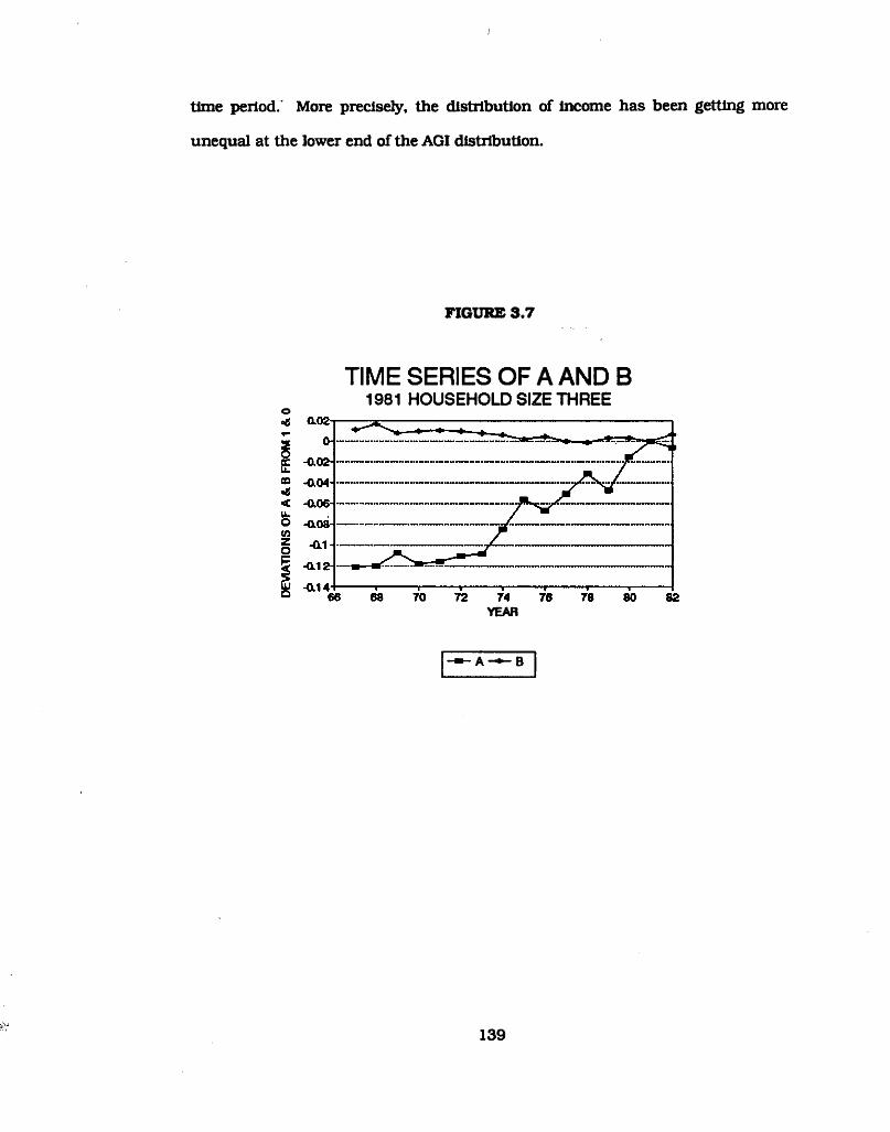
tim e period.* More precisely, the d is trib u tio n o f incom e has been getting more

unequal a t the low er end o f the AG I d is trib u tio n .

FIGURE 3.7

TIME SERIES OF A AND B1981 HOUSEHOLD SIZE THREEO

YEAR

— - A - * - B

139

The functiona l re la tionsh ip between S and T is determ ined fo r each curve

by estim ating Equation (3.1) fo r each year and each household size. However, th is

re la tionsh ip has to be transform ed in to the cum ulative percentages o f popula tion and

the cum ulative percentages o f Incom e, since the Lorenz curve is defined in

percentage term s. The transform ation is done num erica lly. In E quation (3.1),

repeated here fo r easy reference,

T ,h i - AihT81hl ♦ B,h«S,hi>1-5<V'2-S(h() 5) <3 1 >

the constant values o f Shi and the estim ated values o f and Bth fo r each curve and

each year are used to calculate the values o f the transform ed T fo r each year and

each household size. The function is then transform ed to (x,y) coordinates and a

lin e a r in te rp o la tio n is perform ed to provide the equally spaced values o f x and the

corresponding values o f y. These in terpo lated values o f x and y are term ed g rid

values. In p rin c ip le , the num ber o f g rid values determ ines the sm oothness o f the

curve. In ou r m odel, fifty g rid values o f x and y gave a good approxim ation fo r the

curvature o f the Lorenz curve.

C. Forecasting the Incom e D is trib u tio n

To pro ject the Income d is trib u tio n in the fu tu re , the functiona l param eters,

A and B, have to be forecasted. G enerally speaking, A and B m easure the equality

o f the d is trib u tio n o f incom e re la tive to the base year. I f A increases, the Lorenz

curve becomes m ore bowed overall. Namely, the en tire d is trib u tio n o f income

becomes less equal. I f B increases, the curve becomes m ore bowed p a rticu la rly at

the upper end o f the d is trib u tio n . That is , the incom e d is trib u tio n becomes less

equal w ith in the high incom e groups. Thus, increasing e ithe r A o r B w ill increase

140

inequa lity .

In our m odel, the effects o f economic variab les on the incom e d is trib u tio n

are ind ica ted by the m agnitude o f the param eters A and B. For forecasting, A and

B are estim ated as functions o f the econom ic variables and are then used to forecast

the Income d is trib u tio n . To re late A and B to econom ic variab les, the values o f A and

B estim ated from the h is to rica l cross-section data are regressed on unem ploym ent.

In fla tio n and the shares o f In te rest and dividend incom e in to ta l incom e.

In general, the upper incom e groups in an incom e d is trib u tio n receive a

re la tive ly large proportion o f th e ir incom e from investm ent incom e, w h ile the lower

incom e groups earn a re la tive ly high proportion o f th e ir incom e from em ploym ent or

wage incom e. Thus, unem ploym ent w ill probably h it the low income groups hardest.

As fo r in fla tio n , its Influence on the size d is trib u tio n m ay w ork through several

channels, b u t the overall effect is unclear a p rio ri. In o ther w ords, incom es from

d iffe ren t sources respond to a general price increase to d iffe ren t degrees. Since the

proportions o f em ploym ent and investm ent incom e vary over the d is trib u tio n , the

im pact o f in fla tio n on the d is trib u tio n is hard to an ticipate .

We form ulate the param eters A and B as the lin e a r functions o f the

unem ploym ent ra te , the proportion o f net in te rest and dividend incom e in aggregate

personal incom e, the in fla tio n rate , and a tim e trend. The equations estim ated fo r

each household size are w ritte n as

A * Cq * Ci*UN + C2*FC77NC + c3*INFL + c4*T1ME (3.2)

B = do + di*UN * fyPCTINC + dQ*INFL «■ d4*TlME (3.3)

In Equation (3.2) and (3.3), UN is the unem ploym ent ra te ; PCTINC is the percentage

o f aggregate personal income made up o f net in te rest and dividend incom e; INFL is

the annual percentage change in the GNP defla tor; TIM E is the tim e trend ; and the

141

To see how the Income d is trib u tio n is affected by the d iffe ren t variables, we

tu rn to the discussion o f the effects o f the factors on the param eters A and B. The

tim e trend variab le is used in the estim ation equations to catch the secular trends

and separate them from the cyclica l flu c tua tion s. The d is trib u tio n o f income

becomes m ore unequal if incom e is defined to exclude transfe r paym ents. On the

o ther hand, the incom e d is trib u tio n rem ains rough ly constant if the Income concept

includes tra n sfe r paym ents (Pechman, 1985). Thus, we w ould expect the overall

d is trib u tio n o f A djusted Gross Incom e to be less equal over tim e, since transfe r

paym ents are m ostly no t in AGI. That is , the values o f param eter A w ill be

increasing over tim e; and the estim ated coefficient on the tim e trend variab le w ill be

positive. As fo r param eter B, we expect the coefficient o f the tim e trend fo r param eter

B to be negative so th a t the h igher value o f A can be p a rtia lly offset a t the upper end

o f the d is trib u tio n b u t allow s the increase in A fo r the low er p a rt to rem ain, because

we believe th a t the d is trib u tio n o f personal incom e has ra re ly changed and transfe r

paym ents have been accruing a t the low er end o f the d is trib u tio n . In other words,

a negative value fo r the tim e trend coefficient fo r B w ould mean th a t the AGI

d is trib u tio n is getting re la tive ly m ore bowed a t the low er end.

The re la tio n o f unem ploym ent to the incom e d is trib u tio n can be described

by the em pirica l find ings o f M urphy and Topel (1987): "...Persons who experience

unem ploym ent now rem ain unem ployed fo r a m uch longer period, on average, and

persons w ith past unem ploym ent are m ore lik e ly to experience fu tu re unem ploym ent

spells. Both o f the la tte r forces tend to increase inequa lity as unem ploym ent rises."

Therefore, tak ing in to account the facts th a t unem ploym ent m eans low o r no income

and the im pact o f unem ploym ent is greater on low er incom e groups, we expect th a t

unem ploym ent rate Is positive ly correlated w ith A w h ile negatively corre lated w ith B.

q ’s and dj’s are the parameters to be estimated.

142

That is , the Increase in unem ploym ent rate w ill cause the en tire d is trib u tio n to be

m ore unequal, b u t the upper end o f the d is trib u tio n w ill become re la tive ly more

equal.

The percent o f in te rest and dividend incom e in the aggregate personal

incom e is expected to have positive im pact on both A and B. A lthough some aged

persons in the low er Income groups receive re la tive ly large portions o f th e ir income

from the in te rest and dividends, m ost o f th is type Income goes to those in the top

incom e groups. Thus, as the percentage o f net In te rest and dividend income

increases, it is expected th a t the d is trib u tio n o f Income becomes m ore unequal both

fo r the en tire and the upper end o f the d is trib u tio n .

The evidence o f the im pact o f in fla tio n on incom e d is trib u tio n is lim ite d , so

we can ha rd ly id e n tify the expected resu lts. Some studies show th a t in fla tio n has

little effect on the d is trib u tio n o f money incom e (M inarik, 1970), w h ile others indicate

th a t in fla tio n has an adverse effect on some low er incom e groups (M etcalf, 1969).

The h is to rica l values o f the in fla tio n rate together w ith the unem ploym ent

ra te and the share o f net in te rest and dividend incom e in aggregate personal income

are lis te d in Table 3.2. The tim e-series regression resu lts fo r Equation (3.2) and (3.3)

fo r each household size are shown in Table 3.3. M ost o f the estim ated coefficients

have the signs w hich are consistent w ith our p rio r expectations. Table 3.3 shows the

values o f a ll the coefficients and those w hich are s ig n ifica n t a t 10% level are

Indicated by an asterisk (*). In fla tio n is s ig n ifica n t on ly fo r household size one.

Thus, ou r re su lt seems to be close to M ina rik ’s study.

To com plete the pro jection o f the incom e d is trib u tio n , a few other variables

need to be forecasted. In ou r incom e d is trib u tio n m odel, incom e is d is tribu te d over

the popu la tion represented on tax re tu rns w ith positive AGIs. T h is popula tion is

referred to as "to ta l exem ptions", o r m ore precisely to ta l exem ptions o ther than age

143

o r blindness. T h is popula tion has to be forecasted w ith n o n -in s titu tio n a l population.

The forecasts o f "to ta l exem ptions" are shown in Table 3.4. In add ition , the share o f

to ta l popula tion and the share o f to ta l AGI from each o f the household size categories

has to be forecasted. These shares are form ulated as a lin e a r fu n c tio n o f a constant

term and the percent o f the popula tion s ix ty-five years o r older. Th is explanatory

variab le is used because it catches the tim e trend and, m ore im po rtan tly , it provides

reasonable looking forecasts. The forecasting resu lts are represented in Table 3.5

and Table 3.6 respectively.

n . Incom e Tax M odel

The incom e d is trib u tio n m odel has been b u ilt fo r before-tax incom e. For the

consum ption function , we need the d is trib u tio n o f a fte r-ta x incom e. The income tax

m odel provides the way from one to the other.

The basic idea in ca lcu la ting the incom e ta x is to com pute the "standard

taxes" based on the standard deductions, and rates and brackets from the tax form s,

and then to compare these "standard taxes" w ith taxes actua lly collected, the

"effective taxes". In forecasting, we need the tax schedules as found on the tax

re tu rn s , and functions fo r the ra tio o f effective taxes to standard taxes.

In general, "effective" taxes w ill always be less than "standard" taxes. The

fra c tio n o f the effective tax rates to the standard ta x rates varies by incom e ventiles;

m oreover, it changes over tim e. It is expected th a t the la rger discrepancies o f

standard taxes and effective taxes arise in the h igher Income ventiles. In the

h is to rica l w ork, the standard tax rates paid by the average m em ber o f each incom e

group were calculated by assum ing th a t th is average household takes the standard

deduction and has no o ther special item s. These taxes were com puted by using the

ta x rate schedules in the form 1040.

The effective tax rates, on the o ther hand, were calcula ted by d iv id ing the

am ount o f incom e taxes by the am ount o f AG I in each bracket reported in SOI.

These rates were then lin e a rly in terpo la ted to get a d is trib u tio n over the tw enty

incom e ventiles. Both the standard and the actua l tax rates were calculated fo r each

household size separately.

Since the consum ption functions do no t require the d is trib u tio n o f incom e

by household size, the standard and effective taxes d is trib u tio n were collapsed to a

single d is trib u tio n o f these taxes by income per capita . Thus, the tax m odel

estim ates the ra tio s o f effective-to-standard tax rates fo r each o f the tw enty ventiles

in the single d is trib u tio n o f incom e, not fo r tw enty ventiles fo r each o f s ix household

sizes. These ra tio s are to be used in forecasting.

How is th is collapsing from six to one d is trib u tio n s done? The fundam ental

procedure is to obta in the single d is trib u tio n o f incom e by determ ining the cu to ff per

cap ita incomes in the aggregate ventiles. We define cu to ff per capita incom e as the

upper bound o f per capita incom e in th a t incom e ven tile . Since the no tion o f the

cu to ff incom es w ill be repeatedly used in the fo llow ing, we w ill derive here the cu to ff

incom es fo r easy reference.

Before ca lcu la ting the c u to ff incom es, we w ill in troduce some de fin itions to

be used in the com putation. F irs tly , we w ill convert the percentages o f popula tion

and incom e in our incom e d is trib u tio n s in to the num ber o f people and the do lla r

am ount o f incom e fo r each year and each household size in each g rid ce ll. To make

th is transform ation , le t X ^g be the num ber o f in d iv idua ls and Y ^g be the do lla r

am ount o f income fo r year t, household size h , and g rid ce ll g. F u rthe r, we assume

th a t is the to ta l num ber o f popula tion and is the to ta l am ount o f incom e fo r

year t and household size h. Thus, the form ulas can be w ritte n as follow s:

145

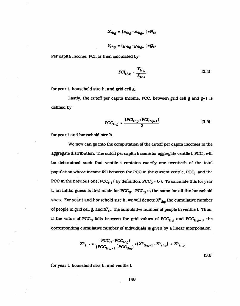
^thg ° x̂ thg~xth g -0 *^ th

Ythg = lythg~ythg-l)*Qth

Per capita Income, PCI, is then calculated by

(3.4)

fo r year t, household size h , and g rid ce ll g.

Lastly, the c u to ff per capita incom e, PCC, between g rid ce ll g and g+1 is

defined by

fo r year t and household size h.

We now can go in to the com putation o f the cu to ff per cap ita incom es in the

aggregate d is trib u tio n . The c u to ff per capita income fo r aggregate ven tlle i, PCCj, w ill

be determ ined such th a t ven tlle i contains exactly one tw entie th o f the to ta l

pop u la tion whose Income fe ll between the PCC in the cu rre n t ventlle , PCClt and the

PCC in the previous one, PCCj. x ( By d e fin itio n , PCC0 = 0 ). To calculate th is fo r year

t, an in itia l guess is firs t made fo r PCCti. PCCti Is the same fo r a ll the household

sizes. For year t and household size h , we w ill denote ^ th g cum ulative num ber

o f people in g rid ce ll g, and the cum ulative num ber o f people in ventlle i. Thus,

i f the value o f PCCti fa lls between the g rid values o f PCCthg and PCCthg+ j , the

corresponding cum ulative num ber o f Ind ividua ls is given by a lin e a r in te rpo la tion

(3.5)

(PCCt r PCCthg)+ x cthg

(3.6)

fo r year t, household size h, and ventlle 1.

146

Therefore, the num ber o f people in the 1th ventile o f household size h in year

t. X jjjj, is the difference o f and ^ th i- i* ^ t h i' ^ th i- i* T l̂ls has to be done fo r

each year and each household size. The X ^ ’s are then summed over the household

sizes h fo r the given year. I f th is am ount is low er than 5 percent o f the to ta l

popu la tion o f th a t year, another guess is made a t a h igher value o f PCCti. On the

o ther hand. I f th a t sum is greater than 5 percent o f the popula tion. PCCa is lowered

by a sm all am ount. The process is repeated u n til the convergence is achieved. This

approach has to be done fo r each o f the firs t nineteen Income ventiles.

The com puted PCC^’s are then used to determ ine the am ount o f incom e in

ven tile 1 fo r year t and household size h. V ^ . The ca lcu la tion is done by E quation

(3.6) w ith X being replaced by Y. Since the top income ven tile cannot be expressed

by the cu to ff per capita Income, the am ount o f incom e in it fa lls as a residua l. For

the index o f the d is trib u tio n o f incom e, the cu to ff Incom es o f the firs t nineteen

ven tiles are divided by the average incom e, and the top ventile Is represented by an

overa ll percentage o f to ta l Income. The deta ils o f popula tion and incom e d is trib u tio n

fo r the selected years are shown in Table 3.7. Table 3.8 shows the d is trib u tio n o f

ven tile ’s c u to ff per capita AGI. Table 3.9 shows the indexes o f the d is trib u tio n o f AGI

fo r the selected years.

We now tu rn to the forecasting o f effective tax rates. For forecasting, the tax

param eters fo r the standard taxes are given by the tax law assum ptions. The

standard tax rates were calculated fo r each household size, and then aggregated in to

a single rate fo r each Income ventile over the s ix household sizes. The incom e shares

o f the household sizes were the weights fo r the weighted-average scheme. The

estim ated ra tio s o f effective-to-standard tax rates were then applied to the aggregate

d is trib u tio n o f the standard tax rates to obta in the d is trib u tio n o f the effective tax

rates.

147

The forecasted effective ta x rates were incorporated in the aggregate

d is trib u tio n o f AGI to determ ine the a fte r-ta x AG I d is trib u tio n . To provide the

effective ta x rates a t c u to ff incom es, a lin e a r in te rpo la tion was perform ed. The

effective ta x rates a t c u to ff incom es were then used to remove federal incom e taxes

from the c u to ff AG Is. Table 3.10 shows the average effective and standard tax rates

fo r some selected incom e ventiles. Table 3.11 represents the estim ated ra tios o f

effective-to-standard tax rates.

m . D is trib u tio n o f Disposable Incom e

A. A d justm ent Between AGI and PI

The SOI data used fo r estim ating income d is trib u tio n is AGI. In the

consum ption m odel, however, consum ption expenditures are determ ined by the level

o f personal incom e. More specifica lly, it is the disposable personal income th a t

affects the consum ption tendencies. However, if we can get the d is trib u tio n o f PI, we

can use ou r tax function to convert it to disposable personal incom e. Therefore, we

have to reconcile between the d is trib u tio n o f AGI and the d is trib u tio n o f PI.

The differences between AGI and PI come from several item s. Table 8.14 in

N ational Incom e and Product Accounts (NIPA) shows the de ta ils o f the re la tionsh ip

between PI and AGI. We rearrange those divergences by com bining some and

disaggregating others. In our m odel the reconcilia tion Item s are sum m arized by 12

categories. The firs t five categories are the item s o f tran sfe r paym ents. They are: 1)

OASDI - O ld age, survivors and d isa b ility insurance, 2) H I - H ospita l and

supplem entary m edical insurance, 3) U I - Unem ploym ent insurance, 4) RET -

R etirem ent Income and other item s, and 5) WELF - W elfare and a ll the o ther m eans-

148

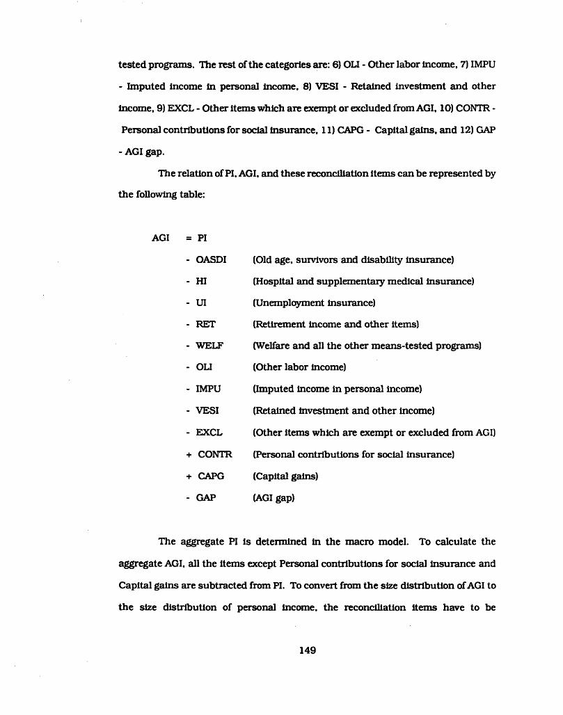
tested program s. The rest o f the categories are: 6) OLI - O ther labor incom e, 7) IMPU

- Im puted incom e in personal Incom e, 8) VESI - Retained investm ent and other

incom e, 9) EXCL - O ther item s w hich are exem pt o r excluded from AG I, 10) CONTR -

Personal con tribu tions fo r social insurance, 11) CAPG - C apita l gains, and 12) GAP

- AG I gap.

The re la tio n o f PI. AG I, and these reconcilia tion item s can be represented by

the fo llow ing table:

= PI

- OASDI (O ld age, survivors and d isa b ility insurance)

- H I (H ospital and supplem entary m edical Insurance)

- U I (Unem ploym ent Insurance)

- RET (Retirem ent incom e and other item s)

- WELF (W elfare and a ll the o ther m eans-tested program s)

- OLI (O ther labor income)

- IMPU (Im puted income in personal income)

- VESI (Retained investm ent and o ther income)

- EXCL (O ther item s w hich are exem pt o r excluded from AGI)

+ CONTR (Personal con tribu tions fo r social Insurance)

+ CAPG (C apita l gains)

- GAP (AGI gap)

The aggregate PI is determ ined in the m acro m odel. To calculate the

aggregate AG I, a ll the item s except Personal con tribu tions fo r social insurance and

C ap ita l gains are subtracted from PI. To convert from the size d is trib u tio n o f AGI to

the size d is trib u tio n o f personal Incom e, the reconcilia tion item s have to be

149

forecasted in d iv id u a lly and then d is trib u te d over the tw enty incom e ventiles. The

forecasts in the reconcilia tion item s are presented in the fo llow ing section.

According to NIPA table 3.11, transfe r paym ents are composed o f twelve

p rin c ip a l elem ents. The twelve tran sfe r paym ent com ponents are form ulated

in d iv id u a lly in the m acro m odel as a function o f tim e, the price level, and the

popu la tion aged 65 and over and are forecasted separately a t the aggregate level.

F u rthe r, some o f the forecasted item s are com bined In to one category and others are

used in d iv id u a lly to provide ou r five tran sfe r paym ent categories. The re la tionsh ip

between the tran sfe r paym ent com ponents in NIPA table 3.11 along w ith the

reconcilia tion item s from NIPA table 8.14 and ou r de fin ition s fo r reconcilia tion item s

is shown in Table 3.12. The NIPA tables 3.11 and 8.14 are reproduced in Figure 3.8

and Figure 3.9 fo r the purpose o f reference.

150

FIGURE 3.8

NIPA Table 3.11

Table 3.11*-̂2ovtnunent Transfer Payments to Person(BOioas o f dotes)

Line 1916 1917 1988 1989

I 496J S21J B7.42 3M4 40U

332*4217373.03 y u p 40: 1

5ft 734I6J1&0

2

>1.914.614.2

.1j

C6.713.613.1

.1

97.9

7 144■

TVAnt — 9 jSnrrhil ^ 10

r iA r tl — - 11 41224.4175

44.926J18.46J1.71.21.0

48.1 2*6 19.36.71.7 1.3 1J

306 29V 207 7.(1 1 * 141.3

CHH-* ‘ 12WMmy* 13

14 641.71.1.9

is ̂ i — - — •-- 16iBIjMY Immwmwmm » 17

**|~ * ---"*-■ 11 14.9142

14.814J

13.014.6

.4

13.313019

■ a 20 .7 JbOtter* 21

. ■___ ____fc- 22 10.6 10.61.3

10.0

11.21.3

10.7

12.21.3

11.623 1.624 »J2326 1A 1.4 2.9

11.440

27 10.1 105 11.92S 1119 119.7 U li

42.6143.9

29 33.921.7

J7.631.4

46930 33.9 39.3

T. .iiii.uu> ------ 31 1J is 1.6 1.8^|T jf rj,« —------ 32 3.9 4.7 3.0 3.6*— 33 70.7 73.6 n o 91.234 43.4 49.8 33.0 62.9

A fat fhnHl̂ y iIhmmIh i rtilA w ii 33 16.4 16.7 17J 18.0* j|-»---- > — t---- ^ 36 2.6 2.9 3.1 3.437 15 2.6 2.7 2.838 2JO 1.7 l.> 1.3Sis 39 1.7 1.9 2.3 2740 35 4.0 4J 4.8 ̂ ■ _ j . • ■ 41 ID .9 .9 1.0

....................... 42 1.3 1.6 1.1 2.0

1. Oom m o f cM auvta . tuwlgi (a v ia . Public Health Sevice o ffiem , Tconcnee Valky A ohoriiy. and m jui I nm ll m iiaum program .

2. Iik M m (he Com (M .1 ttw K a or payment h r metical iw tc u h i dtptm him o f a n te doty m ilitary penonnel at

•oBnUinrv ficilm ei4. Ooamtt of cm pay, m iiaa l leave pay, end adjuurd compt na tion benefits.3. Caaaa largely of payments m Moprofu hwrinitiom. aid to Mudema, and paymenn tor medial service*

h r w iiu i mQitny penotmd and tfccfr dependents ai nonmiliiary facilities.6. Cbnbts « f in>rgm ry an ln s r r and medical im urw e premium payments paid oa behalf o f indigents7. Cbaata >B|dy o f foster caie, w n m benefits, Ahsk* d ividends, and crime victim payments.

151

FIGURE 3.9

NIPA Table 8.14

Table 8.14.—Comparison of Personal Income in the National Income and Product Accounts (NIPA’s) with Adjusted Gross Income as Published by the Internal Revenue Service (IRS)

(Billion) of dotlan)

Line 1986 1987 1988 1989

Wmaaat Income, NIPA's.......................................................... 1 XS26J 3.76M 4J70J 1 TH t2 1.100.6 1X193.9 1.133.7

Transfer payments except ta**ble m ilitiry rctimneni and 3 440J 438.4 486Jtaxable government pensions.

Other labor income except fees __ ___ - ..... 4 193.7 203.3 221.2Imputed income in personal income - ___ —...... ... 3 71.1 87.1 87.4 126investment income of life insurance carriers and private 6 119.0 136.2 148.7 161.9

noninsured pension plansInvestment income received by nonprofit institutions or 7 13.0 33.4 36J

retained by fiduciaries.Differences in accounting oeamem between NIPA's and I 97.7 108.1 109.9

ox regulations, netOther personal income exempt or excluded from adjusted 9 143 J 63J 63.6

gi ou InromtPhtt' of aitivtm l § .....mi ^ inrluift H in penonal 10 397J 4)2.0 JSOJ

income.Penonal contributions for aodal insurant________ -__ II 161.9 172.9 194.1 212.8Net gain from ale of assets _____ 12

])133.694.1

138.0110.0

l6S.fi 127 A

---------

14 7.3 17.9 99.813 A -6.9 23.2

Eqsab: BEA-derived a^JaHed groaa (neoene------------------------- 16 24234 3,104.4 U tlAAdjusted pvaa te o iw , IRS______ ___ ___________________ 17 X4S1.7 2.T71* 3,130.7 _Adjusted grses bacon* (AGI) p p ] ------------------------ ----- - 18 J41.7 ] » i 336.7

AGI gap (line 18) as a percentage of BEA-derived AOl 19 12.1 10.6 9.7 -----|UBS JO)>

AGI of RS (tine 17) aa a pejrema** of BEA-derived AGI 20 87.9 89.4 90J ... ..(Hne 16).

I. Equate imputed interest received by paten front life instance earrien and private nooinsuml pension plans u shown in able 8 J (line 30).

1 Consists of income tu ned by low-income Individuals who m not required to file income a * rm rn i unit ported income thu is included in the NIPA measure. and crocs erron and oenissions in lines 2 through 13. Also includes the nei effect of erron in the IRS adjusted gross income (line IT) and NIPA personal income (line I) measure*. Such erron can arise ftwn the sample used by IRS to estimate line 1? and from the d in aoutcts used by BEA to estimate line 1.

152

T he 'sixth reconcilia tion item , other labor incom e, Is estim ated as a function

o f labo r com pensation fo r private w orkers, federal w orkers, and state and local

governm ent w orkers. Those labor com pensation categories are forecasted in the

m acro m odel. The next item , im puted incom e in personal incom e, is estim ated as

a fu n c tio n o f In te rest Income, the m ortgage ra te , and tim e. In te rest incom e and the

m ortgage ra te are also forecasted in the m acro m odel.

The eighth item , reta ined investm ent and o ther incom e, is calculated as a

fu n c tio n o f tre a su ry -b ill ra te , personal incom e, and tim e. The n in th item , other item s

w h ich are exempt o r excluded from AG I, is calculated as a fixed percentage o f

personal incom e. The fo llow ing item , personal co n trib u tio n fo r social insurance, is

calculated as a fun ctio n o f priva te labor com pensation.

C apita l gains are forecasted by the variab le o f the AAA bond ra te m inus the

lagged percent change In the GNP de fla to r and PI. The la s t item , the AGI gap, is

estim ated to be a fla t percentage o f PI. The estim ation resu lts o f the reconcilia tion

item s other than transfe r paym ents are shown in Table 3.13.

The next step is to transform the aggregate am ount o f the reconcilia tion

item s In to the size d is trib u tio n . The conversion from the d is trib u tio n o f AGI to the

d is trib u tio n o f PI is to add to each AGI ventile ’s PCCU the corresponding aggregate

am ount o f the per capita reconcilia tion cutoffs. Therefore, the d is trib u tio n o f each

o f the reconcilia tion item s over tw enty income ventiles has to be determ ined.

In the m odel, the size d is trib u tio n o f reconcilia tion item s are e ithe r assumed

to be id en tica l o r s im ila r to th a t o f AGI or derived from the p a rticu la r data sources.

The d is trib u tio n o f U I (unem ploym ent Insurance), CAPG (cap ita l gains), and RET

(retirem ent income) were constructed by the data reported in SOI by AGI bracket.

The d is trib u tio n o f OASDI (old age, survivors and d is a b ility income) and WELF

(welfare) were obtained by using the data reported by the Census Bureau and Social

153

S ecurity A dm in istra tion . H I (hospita l and supplem entary m edical insurance) was

assum ed to be d is tribu te d equally over the tw enty income ventiles. EXCL (exclusion)

was assum ed to be d is tribu te d less equally than cap ita l gains. CONTR (contribu tions

fo r social insurance) was assumed to be d is trib u te d m uch like AGI except the top two

ventiles. VESI (retained investm ent income) was assumed to be d is trib u te d s im ila rly

as pension and ann u ity incom e. OLI (other labor Income), IMPU (im puted income),

and GAP (AGI gap) were assumed to be d is tribu te d in a s im ila r pa tte rn w ith AGI.

The re su ltin g d is trib u tio n s are represented by a m a trix whose colum ns conta in the

share o f each item going to each ven tile .2 The m a trix is shown in Table 3.14.

To calculate the aggregate am ount o f per capita reconcilia tion cu to ffs, the

vector o f reconcilia tion item s is m u ltip lie d by the corresponding colum n o f the

in d iv id u a l shares. Thus, sum m ing over the twelve item s fo r each o f the ventiles. we

m ay ob ta in a 20x 1 vector w ith each elem ent representing the to ta l d o lla r am ount o f

the reconcilia tion item s fo r th a t ventile . The per capita cu to ff reconcilia tion is then

determ ined by a lin e a r in te rpo la tion and is added to the corresponding AGI c u to ff by

the incom e d is trib u tio n m odel.

B. D is trib u tio n o f Disposable PI

To generate the d is trib u tio n o f a fte r-ta x AG I, a ll the taxes have to be

removed. Federal incom e taxes a t each cu to ff incom e are determ ined by m u ltip ly in g

the p re -tax cu to ff AG I by the effective tax rates on th a t c u to ff incom e. The effective

ta x rates a t the cu to ff incom e level are calculated by lin e a r in te rpo la tion . F urther,

fo u r o ther types o f personal taxes need to be removed. They are: State and local

incom e taxes. State and local o ther taxes. Federal nontaxes, and State and local

2This m atrix, reconciliation bridge, was derived in Pollock (1986).

154

nontaxes. In ou r ta x m odel, state and loca l incom e ta x is calculated as a fixed

percentage o f federal incom e taxes, and other taxes are calculated as percentages o f

personal incom e.

The d is trib u tio n o f disposable PI can then be obtained by adding the

aggregate am ount o f per capita reconcilia tion cu to ffs to the corresponding a fte r-tax

AG I cu to ffs. However, an adjustm ent m ust be made fo r the cu to ff P i's. The

popu la tion reported by the IRS contains only the tax file rs who have positive AGIs.

In ou r consum ption m odel, we need the d is trib u tio n o f disposable personal incom e

over the en tire popula tion. The h is to rica l data show th a t about 7.5 percent o f the

to ta l popu la tion was le ft ou t o f the popula tion in SOI. Thus, le t vt be the unadjusted

and Vj* the adjusted cu to ff incom e fo r ventile i, the adjustm ent can be expressed as

follow s

Uj* ■ .65

vi = y n “ (-075 * (2 0 -< )- l) * (u i_1-u f_2) i - 3 .....6 (3*®)

vtm = ut - .0 7 5 *(2 0 - i)* (u t -u t_1) i=7 .....19 (3 -9)

The adjusted c u to ff incom e fo r the firs t ventile is com puted by the census

data on m oney Income. As fo r the top incom e ven tile , the num ber o f ind iv idua ls in

th is ven tile is increased by p a rt o f the tax file rs who were in the nineteenth ventile .

Thus, the p roportion o f incom e received by the in d iv idua ls in the adjusted top income

ven tile in to ta l incom e w ill increase by about 7.5 percent.

F in a lly , an index o f disposable personal incom e d is trib u tio n has to be

constructed fo r use in the consum ption m odel. The index fo r the firs t nineteen

ven tiles is defined as the cu to ff per capita personal income divided by the average per

155

capita personal incom e. H ie tw entie th index is defined as an overall average o f the

to ta l personal Incom e. Table 3.15 shows the Indexes fo r some selected years.

156

TABLE 3.1

Estimation Results for Parameters A and B

YEAR 1966 HH SIZE 1 I YEAR 1966 HH SIZE 2 1 YEAR 1966 HH SIZE 3RSQ 0. 9977 RBARSQ 0.9976 1 RSQ 0 .9980 RBARSQ 0.9979 IRSQ 0. 9960 RBARSQ 0 .9959RHO 0. 9191 MAPE 2.9376 I RHO 0 .7895 MAPE 1.3637 IRHO 0. 8620 MAPE 2 .3768A 1. 0024 T-STAT 152.20 |A 0 .9737 T-STAT 175.82 IA 0. 8791 T-STAT 129.28B 0. 0254 T-STAT 8.24 IB 0 .0013 T-STAT 0.60 IB 0. 0113 T-STAT 4.73

YEAR 1966 HH SIZE 4 1 YEAR 1966 HH SIZE 5 1 YEAR 1966 HH SIZE 6RSQ 0. 9956 RBARSQ 0.9954 I RSQ 0 .9963 RBARSQ 0.9962 IRSQ 0. 9946 RBARSQ 0 .9944RHO 0. 5675 MAPE 2.1708 1 RHO 0 .4519 MAPE 2.0788 IRHO 0. 6079 MAPE 3 .0645A 0. 8655 T-STAT 118.50 |A 0 .8573 T-STAT 124.24 IA 0. 7901 T-STAT 95.50B 0. 0180 T-STAT 7.75 IB 0 .0186 T-STAT 8.41 IB 0. 0216 T-STAT 7.60

YEAR 1968 HH SIZE 1 I YEAR 1968 HH SIZE 2 I YEAR 1968 HH SIZE 3RSQ 0. 9989 RBARSQ 0.9989 I RSQ 0 .9968 RBARSQ 0.9967 IRSQ 0. 9913 RBARSQ 0 .9910RHO 0. 8881 MAPE 1.5134 1 RHO 0 .8905 MAPE 1.6565 IRHO 0. 9393 MAPE 3 .1845A 1. 0181 T-STAT 228.22 IA 0 .9676 T-STAT 138.08 IA 0. 8801 T-STAT 87.97B 0. 0208 T-STAT 9.96 IB 0 .0088 T-STAT 3.15 IB 0. 0162 T-STAT 4.60

YEAR 1968 HH SIZE 4 1 YEAR 1968 HH SIZE 5 I YEAR 1968 HH SIZE 6RSQ 0. 9916 RBARSQ 0.9914 I RSQ 0 .9936 RBARSQ 0.9934 IRSQ 0. 9917 RBARSQ 0 .9915RHO 0. 8964 MAPE 2.9870 I RHO 0 .8814 MAPE 2.5788 IRHO 0. 9151 MAPE 3 .2916A 0. 8688 T-STAT 87.55 IA 0 .8430 T-STAT 92.66 |A 0. 7956 T-STAT 77.93B 0. 0243 T-STAT 7.73 IB 0 .0308 T-STAT 10.37 IB 0. 0269 T-STAT 7.69

YEAR 1969 HH SIZE 1 1 YEAR 1969 HH SIZE 2 I YEAR 1969 HH SIZE 3RSQ 0. 9987 RBARSQ 0.9987 I RSQ 0 .9947 RBARSQ 0.9948 IRSQ 0. 9903 RBARSQ 0 .9900RHO 0. 9054 MAPE 1.6240 I RHO 0 .9192 MAPE 2.0067 IRHO 0. 9194 MAPE 3 .2512A 1. 0215 T-STAT 213.01 IA 0 .9828 T-STAT 114.38 |A 0. 8924 T-STAT 84.93B 0. 0173 T-STAT 7.71 IB -0 .0063 T-STAT -1 .8 4 IB 0. 0079 T-STAT 2.14

YEAR 1969 HH SIZE 4 I YEAR 1969 HH SIZE 5 I YEAR 1969 HH SIZE 6RSQ 0. 9904 RBARSQ 0.9901 I RSQ 0 .9908 RBARSQ 0.9905 IRSQ 0. 9868 RBARSQ 0 .9864RHO 0. 9234 MAPE 3.1548 I RHO 0 .8665 MAPE 3.1815 IRHO 0. 9123 MAPE 3 .9820A 0. 8685 T-STAT 83.46 IA 0 .8483 T-STAT 78.81 IA 0. 8115 T-STAT 63.96B 0. 0166 T-STAT 5.03 IB 0 .0253 T-STAT 7.33 IB 0. 0197 T-STAT 4.54

YEAR 1970 HH SIZE 1 [YEAR 1970 HH SIZE 2 (YEAR 1970 HH SIZE 3RSQ 0. 9993 RBARSQ 0.9992 1 RSQ 0 .9990 RBARSQ 0.9989 1RSQ 0. 9979 RBARSQ 0 .9979RHO 0. 8481 MAPE 1.0799 1 RHO 0 .7542 MAPE 1.2057 IRHO 0. 8058 MAPE 1 .9257A 1. 0118 T-STAT 287.17 |A 0 .9646 T-STAT 245.98 IA 0. 8824 T-STAT 176.85B 0. 0017 T-STAT 1.05 IB -0 .0026 T-STAT -1 .6 7 IB 0. 0099 T-STAT 5.62

YEAR 1970 HH SIZE 4 1 YEAR 1970 HH SIZE 5 1 YEAR 1970 HH SIZE 6RSQ 0. 9978 RBARSQ 0.9977 1 RSQ 0 .9979 RBARSQ 0.9978 1RSQ 0. 9977 RBARSQ 0 .9976RHO 0. 6584 MAPE 1.6616 1 RHO 0 .6288 MAPE 1.3586 IRHO 0. 6911 MAPE 2 .0974A 0. 8755 T-STAT 166.01 |A 0 .8985 T-STAT 165.83 IA 0. 8491 T-STAT 150.29B 0. 0163 T-STAT 9.69 IB 0 .0150 T-STAT 8.57 IB 0. 0154 T-STAT 7.88

YEAR 1971 HH SIZE 1 1 YEAR 1971 HH SIZE 2 [YEAR 1971 HH SIZE 3RSQ 0. 9993 RBARSQ 0.9993 I RSQ 0 .9988 RBARSQ 0.9987 IRSQ 0. 9982 RBARSQ 0 .9982RHO 0. 8351 MAPE 1.0061 1 RHO 0 .8079 MAPE 1.4283 1RHO 0. 7961 MAPE 1 .3183A 1. 0106 T-STAT 294.19 |A 0 .9590 T-STAT 223.78 IA 0. 8844 T-STAT 191.79B 0. 0050 T-STAT 3.10 IB -0 .0020 T-STAT -1 .1 8 IB 0. 0107 T-STAT 6.60

YEAR 1971 HH SIZE 4 1 YEAR 1971 HH SIZE 5 I YEAR 1971 HH SIZE 6RSQ 0. 9981 RBARSQ 0.9980 1 RSQ 0 .9984 RBARSQ 0.9984 1RSQ 0. 9979 RBARSQ 0 .9978RHO 0. 5579 MAPE 1.4739 1 RHO 0 .4606 MAPE 1.1835 IRHO 0. 6807 MAPE 2 .1363A 0. 9000 T-STAT 180.83 1A 0 .9194 T-STAT 194.81 IA 0. 8658 T-STAT 158.26B 0. 0151 T-STAT 9.52 IB 0 .0141 T-STAT 9.27 IB 0. 0157 T-STAT 8.31

157

TABLE 3.1

E stim a tion R esults fo r Param eters A and B (C ontinued)

YEAR 1972 HH SIZE 1RSQ 0 .9995 RBARSQ 0.9995RHO 0 .8311 MAPE 1.3489A 1 .0200 T-STAT 345.39B 0 .0008 T-STAT 0.55

YEAR 1972 HH SIZE 4RSQ 0 .9986 RBARSQ 0.9986RHO 0 .4009 MAPE 1.3960A 0 .8951 T-STAT 215.01B 0 .0155 T-STAT 11.66

YEAR 1973 HH SIZE 1RSQ 0 .9995 RBARSQ 0.9994RHO 0 .8335 MAPE 1.3485A 1 .0163 T-STAT 333.80B 0 .0027 T-STAT 1.93

YEAR 1973 HH SIZE 4RSQ 0 .9981 RBARSQ 0.9980RHO 0 .6354 MAPE 1.7425A 0 .8894 T-STAT 184.83B 0 .0101 T-STAT 6.58

YEAR 1974 HH SIZE: lRSQ 0 .9997 RBARSQ 0.9997RHO 0 .7210 MAPE 0.9930A 1 .0165 T-STAT 476.32B 0 .0007 T-STAT 0.74

YEAR 1974 HH SIZE 4RSQ 0 .9973 RBARSQ 0.9972RHO 0 .7173 MAPE 1.7248A 1 .9123 T-STAT 156.70B 0 .0086 T-STAT 4.65

YEAR 1975 HH SIZE: lRSQ 0 .9998 RBARSQ 0.9998RHO 0 .7668 MAPE 0.9102A 1 .0136 T-STAT 511.76B -0 .0022 T-STAT -2 .3 6

YEAR 1975 HH SIZE 4RSQ 0 .9975 RBARSQ 0.9974RHO 0 .7690 MAPE 1.3978A 0 .9501 T-STAT 165.44B 0 .0058 T-STAT 3.15

YEAR 1976 HH SIZE: lRSQ 0 .9998 RBARSQ 0.9998RHO 0 .2747 MAPE 0.6381A 1 .0046 T-STAT 620.82B -0 .0027 T-STAT -3 .5 8

YEAR 1976 HH SIZE 4RSQ 0 .9971 RBARSQ 0.9970RHO 0 .8159 MAPE 1.7866A 0 .9597 T-STAT 154.91B 0 .0036 T-STAT 1.79

YEAR 1972 HH SIZE 2RSQ 0 .9992 RBARSQ 0.9992RHO 0 .7192 MAPE 1.1668A 0 .9566 T-STAT 276.29B 0 .0001 T-STAT 0.05

YEAR 1972 HH SIZE 5RSQ 0 .9992 RBARSQ 0.9992RHO 0 .3375 MAPE 1.1064A 0 .8842 T-STAT 269.19B 0 .0176 T-STAT 16.68

YEAR 1973 HH SIZE 2RSQ 0 .9991 RBARSQ 0.9990RHO 0 .8470 MAPE 1.1621A 0 .9609 T-STAT 259.51B -0 .0063 T-STAT -4 .2 9

YEAR 1973 HH SIZE 5RSQ 0 .9979 RBARSQ 0.9979RHO 0 .7287 MAPE 1.4209A 0 .9045 T-STAT 168.91B 0 .0159 T-STAT 9.20

YEAR 1974 HH SIZE 2RSQ 0 .9984 RBARSQ 0.9984RHO 0 .7616 MAPE 1.3547A 0 .9587 T-STAT 200.89B -0 .0054 T-STAT -2 .8 5

YEAR 1974 HH SIZE 5RSQ 0 .9970 RBARSQ 0.9970RHO 0 .8084 MAPE 1.5627A 0 .9279 T-STAT 144.41B 0 .0121 T-STAT 5.84

YEAR 1975 HH SIZE 2RSQ 0 .9989 RBARSQ 0.9989RHO 0 .6911 MAPE 0.9148A 0 .9799 T-STAT 244.33B -0 .0083 T-STAT -5 .1 5

YEAR 1975 HH SIZE 5RSQ 0 .9972 RBARSQ 0.9972RHO 0 .8215 MAPE 1.4801A 0 .9637 T-STAT 151.75B 0 .0075 T-STAT 3.65

YEAR 1976 HH SIZE 2RSQ 0 .9990 RBARSQ 0.9990RHO 0 .7718 MAPE 0.9036A 0 .9877 T-STAT 250.80B -0 .0101 T-STAT -6 .4 2

YEAR 1976 HH SIZE 5RSQ 0 .9975 RBARSQ 0.9974RHO 0 .7795 MAPE 1.2468A 0 .9704 T-STAT 159.45B 0 .0050 T-STAT 2.52

YEAR 1972 HH SIZE 3 RSQ 0.9985 RBARSQ 0.9984 RHO 0.8460 MAPE 1.7184 A 0.8900 T-STAT 206.22 B 0.0094 T-STAT 6.20

YEAR 1972 HH SIZE 6 RSQ 0.9979 RBARSQ 0.9979 RHO 0.8013 MAPE 2.1303 A 0.8616 T-STAT 162.15 B 0.0148 T-STAT 8 .05

YEAR 1973 HH SIZE 3 RSQ 0.9987 RBARSQ 0.9986 RHO 0.7979 MAPE 1.4881 A 0.8916 T-STAT 221.60 B 0.0078 T-STAT 5.4 6

YEAR 1973 HH SIZE 6 RSQ 0.9975 RBARSQ 0.9975 RHO 0.8118 MAPE 1.9108 A 0.8635 T-STAT 148.29 B 0.0141 T-STAT 7.01

YEAR 1974 HH SIZE 3 RSQ 0.9976 RBARSQ 0.9975 RHO 0.7666 MAPE 1.7588 A 0.9155 T-STAT 168.71 B 0.0054 T-STAT 2.81

YEAR 1974 HH SIZE 6RSQ 0.9972 RBARSQ 0.9972 RHO 0.8221 MAPE 1.8918 A 0.8798 T-STAT 141.78 B 0.0127 T-STAT 5.91

YEAR 1975 HH SIZE 3RSQ 0.997 9 RBARSQ 0.997 9 RHO 0.7985 MAPE 1.4767 A 0.9440 T-STAT 182.47 B 0.0019 T-STAT 1.03

YEAR 1975 HH SIZE 6RSQ 0.9969 RBARSQ 0.9968 RHO 0.8638 MAPE 1.94 50 A 0.9401 T-STAT 138.06 B 0.0065 T-STAT 2.73

YEAR 1976 HH SIZE 3 RSQ 0.9981 RBARSQ 0.9980 RHO 0.7888 MAPE 1.4527 A 0.9447 T-STAT 188.12 B 0.0009 T-STAT 0.53

YEAR 1976 HH SIZE 6 RSQ 0.9970 RBARSQ 0.9969 RHO 0.7857 MAPE 1.7795 A 0.9329 T-STAT 140.50 B 0.0043 T-STAT 1.88

158

TABLE 3.1

E stim a tion R esults fo r Param eters A and B (C ontinued)

YEAR 1977 HH SIZE 1 I YEAR 1977 HH SIZE 2 I YEAR 1977 HH SIZE 3RSQ 0. 9993 RBARSQ 0.9992 I RSQ 0 .9994 RBARSQ 0.9994 1RSQ 0. 9990 RBARSQ 0.9990RHO 0. 7929 MAPE 1.6768 I RHO 0 .4026 MAPE 0.7927 IRHO 0. 3608 MAPE 0.8874A 0. 9883 T-STAT 282.22 IA 0 .9834 T-STAT 327.04 IA 0. 9493 T-STAT 264.60B -0 . 0002 T-STAT -0 .1 2 IB -0 .0104 T-STAT -8 .6 0 IB 0. 0001 T-STAT 0.07

YEAR 1977 HH SIZE 4 1 YEAR 1977 HH SIZE 5 (YEAR 1977 HH SIZE 6RSQ 0. 9980 RBARSQ 0.9979 1 RSQ 0 .9966 RBARSQ 0.9966 1RSQ 0. 9979 RBARSQ 0.9978RHO 0. 6634 MAPE 1.2446 I RHO 0 .7337 MAPE 1.5245 IRHO 0. 6181 MAPE 1.1751A 0. 9406 T-STAT 182.23 |A 0 .9415 T-STAT 134.92 IA 0. 9725 T-STAT 167.61B 0. 0035 T-STAT 2.12 IB 0 .0052 T-STAT 2.32 IB 0. 0033 T-STAT 1.63

YEAR 1978 HH SIZE 1 I YEAR 1978 HH SIZE 2 I YEAR 1978 HH SIZE 3RSQ 0. 9995 RBARSQ 0.9995 I RSQ 0 .9990 RBARSQ 0.9990 IRSQ 0. 9986 RBARSQ 0.9985RHO 0. 7160 MAPE 1.3619 I RHO 0 .5786 MAPE 0.7821 IRHO 0. 6492 MAPE 1.1773A 0. 9823 T-STAT 349.99 IA 0 .9789 T-STAT 248.79 IA 0. 9683 T-STAT 220.67B -0 . 0011 T-STAT -0 .8 8 IB 0 .0056 T-STAT -3 .5 6 IB -0 . 0019 T-STAT -1 .2 4

YEAR 1978 HH SIZE 4 I YEAR 1978 HH SIZE 5 1 YEAR 1978 HH SIZE 6RSQ 0. 9966 RBARSQ 0.9965 1 RSQ 0 .9959 RBARSQ 0.9958 1RSQ 0. 9970 RBARSQ 0.9969RHO 0. 7191 MAPE 1.6871 1 RHO 0 .5369 MAPE 1.5906 IRHO 0. 5533 MAPE 1.8359A 0. 9426 T-STAT 142.44 |A 0 .9490 T-STAT 122.98 IA 0. 9502 T-STAT 141.68B -0 . 0021 T-STAT -0 .9 7 IB 0 .0042 T-STAT 1.67 IB -0 . 0009 T-STAT -0 .4 1

YEAR 1979 HH SIZE 1 I YEAR 1979 HH SIZE 2 I YEAR 1979 HH SIZE 3RSQ 0. 9998 RBARSQ 0.9998 I RSQ 0 .9994 RBARSQ 0.9994 1RSQ 0. 9988 RBARSQ 0.9988RHO 0. 6773 MAPE 0.5128 I RHO 0 .6534 MAPE 0.7935 1RHO 0. 6711 MAPE 1.1275A 0. 9914 T-STAT 559.59 IA 0 .9805 T-STAT 312.79 IA 0. 9532 T-STAT 241.72B - 0 . 0051 T-STAT -6 .2 3 IB -0 .0005 T-STAT -0 .3 9 IB 0. 0033 T-STAT 2.34

YEAR 1979 HH SIZE 4 1 YEAR 1979 HH SIZE 5 1 YEAR 1979 HH SIZE 6RSQ 0. 9977 RBARSQ 0.9977 I RSQ 0 .9985 RBARSQ 0.9984 IRSQ 0. 9985 RBARSQ 0.9985RHO 0. 6138 MAPE 1.5121 I RHO 0 .6322 MAPE 1.0149 IRHO 0. 7019 MAPE 1.2856A 0. 9464 T-STAT 176.47 IA 0 .9538 T-STAT 204.24 IA 0. 9757 T-STAT 200.95B 0. 0038 T-STAT 2.24 IB 0 .0102 T-STAT 6.75 IB 0. 0105 T-STAT 6.18

YEAR 1980 HH SIZE 1 I YEAR 1980 HH SIZE 2 I YEAR 1980 HH SIZE 3RSQ 0. 9999 RBARSQ 0.9999 1 RSQ 0 .9996 RBARSQ 0.9996 IRSQ 0. 9992 RBARSQ 0.9992RHO 0. 3615 MAPE 0.3303 I RHO 0 .3039 MAPE 0.5081 IRHO 0. 3628 MAPE 0.6293A 1. 0030 T-STAT 889.79 IA 0 .9906 T-STAT 384.88 IA 0. 9845 T-STAT 301.91B - 0 . 0007 T-STAT -1 .3 3 IB 0 .0005 T-STAT 0.50 IB 0. 0035 T-STAT 3.01

YEAR 1980 HH SIZE 4 1 YEAR 1980 HH SIZE 5 I YEAR 1980 HH SIZE 6RSQ 0. 9984 RBARSQ 0.9983 I RSQ 0 .9990 RBARSQ 0.9990 1RSQ 0. 9992 RBARSQ 0.9992RHO 0. 5981 MAPE 1.1892 1 RHO 0 .5268 MAPE 0.6725 IRHO 0. 5358 MAPE 0.8314A 0. 9652 T-STAT 209.01 IA 1 .0051 T-STAT 255.50 |A 0. 9755 T-STAT 268.14B 0. 0037 T-STAT 2.53 IB 0 .0092 T-STAT 7.21 IB 0. 0103 T-STAT 8.08

YEAR 1982 HH SIZE 1 I YEAR 1982 HH SIZE 2 [YEAR 1962 HH SIZE 3RSQ 0. 9968 RBARSQ 0.9967 I RSQ 0 .9996 RBARSQ 0.9996 IRSQ 0. 9994 RBARSQ 0.9994RHO 0. 8809 MAPE 3.4056 I RHO 0 .5622 MAPE 0.8070 IRHO 0. 4857 MAPE 0.9196A 0. 9377 T-STAT 124.89 IA 0 .9707 T-STAT 364.66 IA 0. 9938 T-STAT 327.55B 0. 0226 T-STAT 6.52 IB 0 .0089 T-STAT 8.33 IB 0. 0062 T-STAT 5.68

YEAR 1982 HH SIZE 4 I YEAR 1982 HH SIZE 5 1 YEAR 1982 HH SIZE 6RSQ 0. 9993 RBARSQ 0.9993 I RSQ 0 .9993 RBARSQ 0.9993 1RSQ 0. 9994 RBARSQ 0.9994RHO 0. 6251 MAPE 0.9040 1 RHO 0 .7719 MAPE 1.0147 IRHO 0. 8720 MAPE 0.9410A 1. 0116 T-STAT 326.57 IA 1 .0269 T-STAT 305.29 IA 1. 0259 T-STAT 313.11B 0. 0039 T-STAT 3.92 IB 0 .0053 T-STAT 4.80 IB 0. 0084 T-STAT 7.29

159

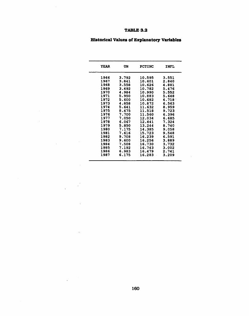
TABLE 3.2

H is to rica l Values o f E xplanatory Variables

YEAR ON PCTINC I NFL

1966 3 .792 10 .595 3 .5511967 3 .841 10.601 2 .8 4 01968 3 .558 10 .626 4 .8 8 11969 3 .49 2 10.782 5 .4 7 61970 4 .984 10.990 5 .5 5 21971 5 .95 0 10.883 5 .6 4 81972 5 .600 10.682 4 .7 1 81973 4 .858 10.872 6 .56 31974 5 .64 1 11.632 8 .9 5 91975 8 .47 5 11.518 9 .72 31976 7 .700 11.560 6 .39 61977 7 .050 12.034 6 .68 51978 6 .067 12.441 7 .3241979 5 .8 5 0 13.244 8 .74 01980 7 .17 5 14 .385 9 .0581981 7 .61 6 15.723 9 .5481982 9.708 16.239 6 .5911983 9.600 16.256 3 .8 8 91984 7 .508 16 .730 3 .7321985 7 .192 16 .743 3 .0021986 6 .983 16 .479 2 .7 4 11987 6 .175 16 .283 3 .2 0 9

160

TABLE 3.3

Tim e-Series Regression R esults o f F unctiona l Param eters fo r Each Household Size

UN PCTINC INFL TIME

A B A B A B A B

z se ho ld> ize

1 .0014 - .0 0 0 0 - . 0 0 8 3 * .0 0 8 6 * .0 0 6 2 * - . 0 0 2 3 * - .0 0 1 7 - . 0 0 3 2 *

2 .0009 - .0 0 0 7 .0022 .0 0 5 3 * .0015 - . 0 0 1 0 .0004 - . 0 0 1 3 *

3 .0018 - .0 0 0 2 .0064 .0 0 2 4 * .0023 - .0 0 0 7 .0 0 5 1 * - . 0 0 1 4 *

4 .0 1 0 5 * - .0 0 0 1 .0 0 7 7 * .0 0 2 3 * .0005 - . 0 0 0 6 .0 0 3 3 * - . 0 0 2 0 *

5 .0 1 4 2 * - . 0 0 2 0 * .0049 .0015 .0020 - . 0 0 0 6 .0 0 4 3 * - . 0 0 1 2 *

6+ .0 0 9 0 * - .0 0 1 2 - .0 0 2 3 .0 0 2 9 * - .0 0 0 7 - .0 0 0 8 .0 1 3 8 * - . 0 0 1 7 *

* S i g n i f i c a n t a t 10% l e v e l .

161

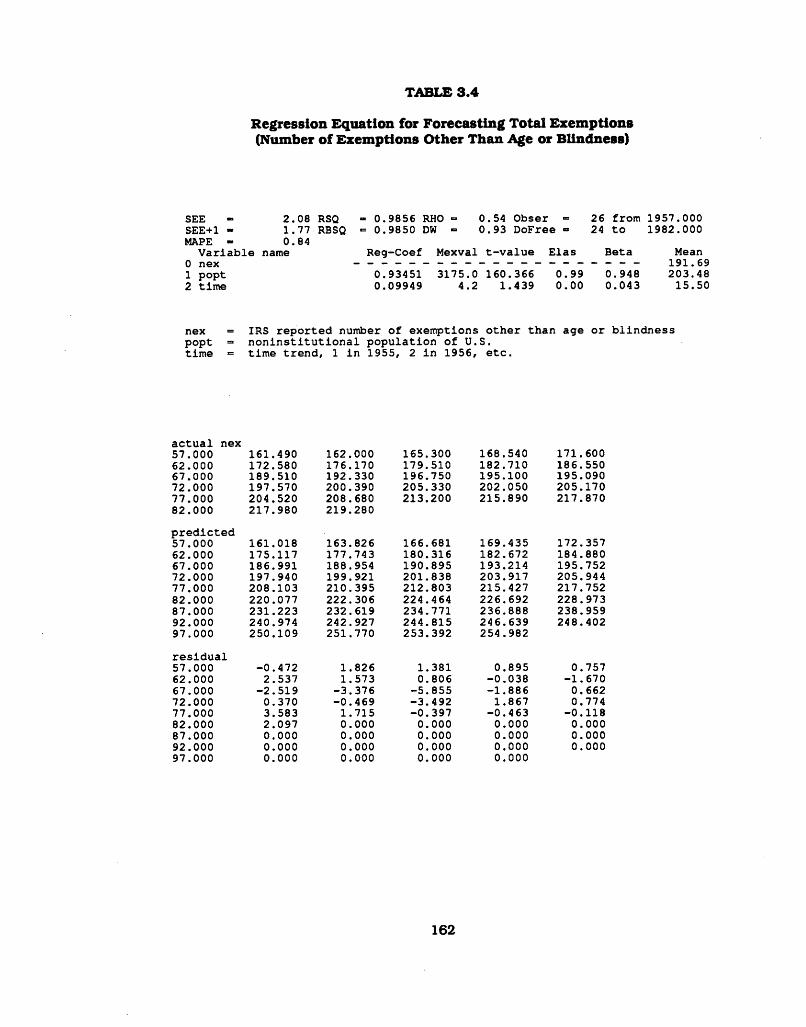
Regression E quation fo r Forecasting T o ta l Exem ptions (Number o f Exem ptions O ther Than Age o r B lindness)

TABLE 3.4

SEESEE+1 - MAPE - 0.84

V a r ia b le name0 nex1 pop t2 t im e

2.08 RSQ 1.77 RBSQ

0.9856 RHO 0.9850 DW

0.54 Obser 0.93 DoFree

Reg-Coef Mexval t - v a lu e E las

0.934510.09949

3175.0 160.366 4 .2 1.439

26 from 1957.00024 t o

Beta

0 .990.00

0.9480.043

1982.000

Mean191.69203.48

15.50

nex = IRS re p o r te d number o f exemptions o th e r than age o r b l in d n e s s pop t = n o n in s t i t u t i o n a l p o p u la t io n o f U.S. t im e *= t im e t re n d , 1 i n 1955, 2 i n 1956, e tc .

a c tu a l nex57.000 161. 490 162. 00062.000 172. 580 176. 17067.000 189. 510 192. 33072.000 197. 570 200. 39077.000 204. 520 208. 68082.000 217. 980 219. 280

p re d ic te d57.000 161. 018 163. 82662.000 175. 117 177. 74367.000 186. 991 188. 95472.000 197. 940 199. 92177.000 208. 103 210. 39582.000 220. 077 222. 30687.000 231. 223 232. 61992.000 240. 974 242. 92797.000 250. 109 251. 770

re s id u a l57.000 - 0 . 472 1. 82662.000 2. 537 1. 57367.000 - 2 . 519 -3 . 37672.000 0. 370 -0 . 46977.000 3. 583 1.,71582.000 2. 097 0.,00087.000 0. 000 0.,00092.000 0. 000 0.,00097.000 0. 000 0. 000

165.300 168.540 171.600179.510 182.710 186.550196.750 195.100 195.090205.330 202.050 205.170213.200 215.890 217.870

166.681 169.435 172.357180.316 182.672 184.880190.895 193.214 195.752201.838 203.917 205.944212.803 215.427 217.752224.464 226.692 228.973234.771 236.888 238.959244.815 246.639 248.402253.392 254.982

1.381 0.895 0.7570.806 -0 .038 -1 .6 70

-5 .855 -1 .8 86 0.662-3 .492 1.867 0.774-0 .397 -0 .4 63 -0 .1 18

0.000 0.000 0.0000.000 0.000 0.0000.000 0.000 0.0000.000 0.000

162

R esults o f Forecasting the Share o f T o ta l P opulation fo r Each o f the Household Size Categories

TABLE 3.5

SEESEE+1 -MAPE =

0.43 RSQ 0.39 RBSQ 2.43

V a r ia b le name0 r n e x l1 in t e r c e p t2 rcpop65

0.9437 RHO 0.9397 DW

0.41 Obser = 1.18 DoFree =

16 fro m 1967.00014 t o 1982.000

Reg-Coef Mexval t - v a lu e Elas

44.04338-2.93225

548.2 23.962 321.6 -15 .325

2.76-1 .7 6

Beta

0.000-0 .971

Mean 15.93

1 . 0 0 9.59

r n e x l == the share o f p o p u la t io n from household s iz e onercpop65 = r e c ip r o c a l o f th e p e rcen t o f the p o p u la t io n 65 years o r o ld e r

a c tu a l rn e x l67.000 13.390 14.130 14.290 13.610 13.62072.000 14.610 15.480 15.950 15.630 16.17077.000 17.270 17.930 18.290 18.170 18.22082.000 18.110

p re d ic te d67.000 13.313 ' 13.651 13.845 14.141 14.42872.000 14.762 15.177 15.619 16.141 16.57877.000 17.013 17.406 17.788 18.062 18.32082.000 18.627 18.941 19.198 19.458 19.75487.000 20.071 20.482 20.720 20.948 21.12892.000 21.274 21.402 21.491 21.584 21.63297.000 21.614 21.600 21.559 21.543

r e s id u a l67.000 -0 .077 -0 .479 -0 .445 0.531 0.80872.000 0.152 -0 .3 03 -0 .331 0.511 0.40877.000 -0 .257 -0 .524 -0 .502 -0 .108 0.10082.000 0.517 0.000 0.000 0.000 0.00087.000 0.000 0.000 0.000 0.000 0.00092.000 0.000 0.000 0.000 0.000 0.00097.000 0.000 0.000 0.000 0.000

163

TABLE 3.5

Results of Forecasting the Share of Total Populationfor Each of the Household Size Categories

(Continued)

SEE - 0.17 RSQ = 0.9852 RHO = -0 .0 8 Obser = 16 from 1967.000SEE+1 - 0.17 RBSQ = 0.9841 DW = 2 .16 DoFree = 14 t o 1982.000MAPE « 0.73

V a r ia b le name Reg-Coef Mexval t - v a lu e E las Beta Mean0 rnex2 ------------- ------- ----------------------------- ------- ------- ------- --- -------- 18.951 i n t e r c e p t 40.80329 1421.8 56.817 2 .15 0.000 1.002 rcpop65 -2.27901 720.8 -30 .485 -1 .1 5 -0 .9 93 9.59

rnex2 = th e share o f p o p u la t io n from household s iz e tworcpop65 = r e c ip r o c a l o f th e p e rce n t o f the p o p u la t io n 65 years o r o ld e r

a c tu a l rnex267.000 16.960 17.240 17.500 17.480 17.60072.000 18.080 18.670 18.390 19.170 19.35077.000 19.710 20.110 20.220 20.460 21.05082.000 21.250

p re d ic te d67.000 16.919 17.182 17.333 17.562 17.78572.000 18.045 18.368 18.711 19.117 19.45677.000 19.795 20.100 20.397 20.610 20.81082.000 21.049 21.293 21.493 21.695 21.92587.000 22.172 22.491 22.676 22.853 22.99392.000 23.106 23.206 23.275 23.348 23.38597.000 23.370 23.360 23.328 23.316

r e s id u a l67.000 -0.041 -0 .058 -0 .167 0.082 0.18572.000 -0 .0 35 -0 .302 0.321 -0 .053 0.10677.000 0.085 -0 .010 0.177 0.150 -0 .24082.000 -0 .201 0.000 0.000 0.000 0.00087.000 0.000 0.000 0.000 0.000 0.00092.000 0.000 0.000 0.000 0.000 0.00097.000 0.000 0.000 0.000 0.000

164

TABLE 3.5

Results of Forecasting the Share of Total Populationfor Each of the Household Size Categories

(Continued)

SEESEE+1 =MAPE =

0.16 RSQ 0.16 RBSQ 0.76

V a r ia b le name0 rnex31 In te r c e p t2 rcpop65

0.9667 RHO - 0.9644 DW =

0.09 Obser 1.82 DoFree =

Reg-Coef Mexval t - v a lu e E las

29.70871-1.42797

16 fro m 1967.00014 to 1982.000

1072.0 43.692 1.85 448.4 -20 .174 -0 .8 5

Beta

0.000-0 .9 83

Mean16.021.009.59

rnex3 = the share o f p o p u la t io n from household s iz e th re ercpop65 = r e c ip r o c a l o f th e p e rcen t o f th e p o p u la t io n 65 years o r o ld e r

a c tu a l rnex367.000 14,.790 14,.850 14. 770 15,.010 15..46072.000 15,.460 15,.940 15. 930 16,.160 16..31077.000 16,.590 16,.400 16. 890 17,.150 17..40082.000 17,.170

p re d ic te d67.000 14,,744 14,. 908 15. 002 15,.146 15..28672.000 15..449 15., 651 15. 866 16,.121 16..33377.000 16,.545 16..737 16. 922 17,.056 17..18282.000 17,.331 17..484 17. 609 17,.736 17..88087.000 18..035 18.,234 18. 350 18,.461 18..54992.000 18..620 18..683 18. 726 18..771 18..79597.000 18..786 18.,779 18. 759 18..751

re s id u a l67.000 -0 ,.046 0,,058 0. 232 0,.136 -0 . .17472.000 -0 ,.011 -0 ,.289 -0 . 064 -0 ,.039 0..02377.000 -0 ,.045 0..337 0. 032 -0 ,.094 -0 . ,21882.000 0,,161 0,,000 0. 000 0..000 0.,00087.000 0,.000 0.,000 0. 000 0..000 0.,00092.000 0,.000 0,,000 0. 000 0..000 0.,00097.000 0,.000 0.,000 0. 000 0..000

165

TABLE 3.5

Results of Forecasting the Share of Total Populationfor Bach of the Household Size Categories

(Continued)

SEESEE+1MAPE

0.24 RSQ 0.23 RBSQ 1.00

V a r ia b le name0 rnex41 In te r c e p t2 rcpop65

0.9230 RHO 0.9175 DW

0.30 Obser = 1.41 DoFree =

Reg-Coef Mexval t - v a lu e Elas

33.46344-1.38551

16 fro m 1967.00014 t o 1982.000

776.1 32.566 1.66 260.3 -12 .953 -0 .6 6

Beta

0.000-0 .961

Mean 20 .18

1 . 0 0 9.59

rnex4 = th e share o f p o p u la t io n from household s iz e fo u rrcpop65 «= r e c ip r o c a l o f th e p e rcen t o f th e p o p u la t io n 65 years o r o ld e r

a c tu a l rnex467.000 18.840 18.740 19.000 19.550 19.55072.000 19.920 19.720 19.940 20.670 20.90077.000 20.730 20.750 21.080 20.930 20.94082.000 21.610

p re d ic te d67.000 18.943 19.103 19.195 19.334 19.47072.000 19.628 19.824 20.033 20.279 20.48677.000 20.691 20.877 21.057 21.187 21.30982.000 21.454 21.602 21.724 21.847 21.98687.000 22.137 22.330 22.443 22.550 22.63692.000 22.705 22.765 22.807 22.851 22.87497.000 22.865 22.859 22.839 22.832

re s id u a l67.000 0.103 0.363 0.195 -0 .216 -0 .08072.000 -0 .292 0.104 0.093 -0.391 -0.41477.000 -0 .039 0.127 -0 .0 23 0.257 0.36982.000 -0 .156 0.000 0.000 0.000 0.00087.000 0.000 0.000 0.000 0.000 0.00092.000 0.000 0.000 0.000 0.000 0.00097.000 0.000 0.000 0.000 0.000

166

TABLE 3.5

Results of Forecasting the Share of Total Populationfor Each of the Household Size Categories

(Continued)

SEESEE+1MAPE

0.16 RSQ 0.16 RBSQ 0.96

V a r ia b le name0 rnex51 in t e r c e p t2 rcpop65

0.9735 RHO 0.9716 DW

0.13 Obser *= 1.74 DoFree =

16 fro m 1967.00014 t o 1982.000

Reg-Coef Mexval t - v a lu e Elas

-2.09087 1.66359

27.6 -2 .967 -0 .1 5 514.2 22.675 1.15

Beta

0.0000.987

Mean13.861.009.59

rnex5 = th e share o f p o p u la t io n from household s iz e f i v ercpop65 = r e c ip r o c a l o f th e pe rcen t o f th e p o p u la t io n 65 years o r o ld e r

a c tu a l rnex567.000 15.340 15.060 14.740 14.930 15.05072.000 14.710 14.060 14.050 13.770 13.69077.000 13.170 12.910 12.720 12.760 12.63082.000 12.160

p re d ic te d67.000 15.344 15.152 15.042 14.874 14.71172.000 14.522 14.286 14.035 13.739 13.49277.000 13.245 13.022 12.805 12.649 12.50382.000 12.329 12.151 12.005 • 11.857 11.69087.000 11.509 11.277 11.142 11.012 10.91092.000 10.827 10.754 10.704 10.651 10.62497.000 10.635 10.642 10.666 10.675

r e s id u a l67.000 0.004 0.092 0.302 -0 .0 56 -0 .3 3972.000 -0 .188 0.226 -0 .0 15 -0 .031 -0 .19877.000 0.075 0.112 0.085 -0 .111 -0 .12782.000 0.169 0.000 0.000 0.000 0.00087.000 0.000 0.000 0.000 0.000 0.00092.000 0.000 0.000 0.000 0.000 0.00097.000 0.000 0.000 0.000 0.000

167

TABLE 3.5

Results of Forecasting the Share of Total Populationfor Each of the Household Size Categories

(Continued)

SEESEE+1MAPE

0.29 RSQ 0.28 RBSQ 1.52

V a r ia b le name0 rnex61 in t e r c e p t2 rcpop65

0.9942 RHO 0.9938 DW

0.27 Obser = 1.45 DoFree =

Reg-Coef Mexval t - v a lu e Elas

-45.838356.35227

887.8 -36.771 1212.1 48.951

16 fro m 1967.00014 t o 1982.000

-3 .044.04

Beta

0.0000.997

Mean15.071.009.59

rnex6 = th e share o f p o p u la t io n from household s iz e s ix o r more rcpop65 = r e c ip r o c a l o f th e pe rcen t o f the p o p u la t io n 65 years o r o ld e r

a c tu a l rnex667.000 20.680 19.980 19.710 19.420 18.73072.000 17.220 16.120 15.750 14.590 13.58077.000 12.520 11.900 10.800 10.530 9.75082.000 9.780

p re d ic te d67.000 20.733 20.002 19.581 18.941 18.31972.000 17.596 16.696 15.738 14.608 13.66277.000 12.719 11.868 11.041 10.446 9.88882.000 9.222 8.543 7.985 7.421 6.78187.000 6.093 5.204 4.689 4.195 3.80492.000 3.488 3.210 3.018 2.816 2.71297.000 2.752 2.782 2.872 2.905

re s id u a l67.000 0.053 0.022 -0 .129 -0 .479 -0 .41172.000 0.376 0.576 -0 .012 0.018 0.08277.000 0.199 -0 .032 0.241 -0.084 0.13882.000 -0 .558 0.000 0.000 0.000 0.00087.000 0.000 0.000 0.000 0.000 0.00092.000 0.000 0.000 0.000 0.000 0.00097.000 0.000 0.000 0.000 0.000

168

TABLE 3.6

R esults o f Forecasting the Share o f T o ta l AGI fo r Each o f the Household Size Categories

SEE - 0.32 RSQ - 0.9769 RHO - 0.57 Obser = 16 from 1967.000SEE+1 = 0.28 RBSQ = 0.9753 DW = 0.86 DoFree = 14 t o 1982.000MAPE = 1.46

V a r ia b le name Reg-Coef Mexval t - v a lu e E las Beta Mean0 r a g i l ---------------------------------------------------------------------------- 19.301 i n t e r c e p t 53.24560 923.0 38.094 2 .76 0.000 1.002 rcpop65 -3.54080 558.0 -24 .335 -1 .7 6 -0 .9 88 9.59

r a g i l = th e share o f t o t a l AGI from household s iz e onercpop65 = r e c ip r o c a l o f th e pe rcen t o f th e p o p u la t io n 65 years o r o ld e r

a c tu a l r a g i l67.000 16.600 17.020 17.040 17.040 16.94072.000 17.790 18.070 19.000 19.020 19.58077.000 20.520 21.130 21.730 21.980 22.52082.000 22.770

p re d ic te d67.000 16.138 16.546 16.780 17.137 17.48472.000 17.887 18.388 18.922 19.553 20.08077.000 20.605 21.080 21.541 21.872 22.18382.000 22.555 22.933 23.244 23.558 23.91587.000 24.299 24.794 25.081 25.356 25.57492.000 25.751 25.906 26.013 26.125 26.18497.000 26.161 26.144 26.094 26.076

re s id u a l67.000 -0 .462 -0 .474 -0 .260 0.097 0.54472.000 0.097 0.318 -0 .078 0.533 0.50077.000 0.085 -0 .050 -0 .189 -0 .108 -0 .33782.000 -0 .2 15 0.000 0.000 0.000 0.00087.000 0.000 0.000 0.000 0.000 0.00092.000 0.000 0.000 0.000 0.000 0.00097.000 0.000 0.000 0.000 0.000

169

TABLE 3.6

Results of Forecasting the Share of Total AGIfor Each of the Household Size Categories

(Continued)

SEESEE+1 =MAPE =

0.23 RSQ 0.23 RBSQ 0.67

V a r ia b le name0 ra g i21 i n t e r c e p t2 rcpop65

0.9595 RHO 0.9566 DW

0.17 Obser <= 1.66 DoFree =

Reg-Coef Mexval t - v a lu e E las

4 5.41847 -1.88145

16 fro m 1967.00014 t o 1982.000

1126.9 45.754 1 .66 396.8 -18 .207 -0 .6 6

Beta

0.000-0 .9 80

Mean27.381.009.59

ra g i2 *= th e share o f t o t a l AGI from household s iz e tworcpop65 = r e c ip r o c a l o f th e p e rcen t o f the p o p u la t io n 65 years o r o ld e r

a c tu a l ra g i267.000 25.720 25,. 900 26.380 25.960 26.36072.000 26.620 27,.300 27.010 27.580 27.63077.000 27.790 28..200 28.310 28.620 29.13082.000 29.560

p re d ic te d67.000 25.701 25,,918 26.042 26.232 26.41672.000 26.630 26.,897 27.180 27.515 27.79577.000 28.075 28.,327 28.572 28.748 28.91382.000 29.110 29.,312 29.477 29.644 29.83387.000 30.037 30., 300 30.453 30.599 30.71592.000 30.809 30.,891 30.948 31.008 31.03997.000 31.027 31.,018 30.991 30.981

r e s id u a l67.000 -0 .0 19 0.,018 -0 .338 0.272 0.05672.000 0.010 -0 . ,403 0.170 -0 .0 65 0.16577.000 0.285 0.,127 0.262 0.128 -0 .21782.000 -0 .450 0..000 0.000 0.000 0.00087.000 0.000 0.,000 0.000 0.000 0.00092.000 0.000 0.,000 0.000 0.000 0.00097.000 0.000 0.,000 0.000 0.000

170

TABLE 3.6

Results of Forecasting the Share of Total AGIfor Bach of the Household Size Categories

(Continued)

SEESEE+1MAPE

0.14 RSQ 0.14 RBSQ 0.70

V a r ia b le name0 ra g l31 in te r c e p t2 rcpop65

0.4368 RHO 0.3965 DW

0.15 Obser 1.71 DoFree

Reg-Coef Mexval t - v a lu e E las

18.75244-0.21218

716.433.2

16 fro m 1967.00014 t o 1982.000

30.315 1.12 -3 .2 9 5 -0 .1 2

Beta

0.000-0 .661

Mean16.721.009.59

ra g i3 = th e share o f t o t a l AGI from household s iz e th re ercpop65 = re c ip ro c a l o f th e p e rc e n t o f th e p o p u la t io n 65 years o r o ld e r

a c tu a l ra g i367.000 16 .570 16. 420 16. 290 16..530 16..82072.000 16 .590 16. 900 16. 770 16..830 16..88077.000 16 .790 16. 590 16.,930 16..910 16.. 94082.000 16 .730

p re d ic te d67.000 16 .529 16. 553 16., 567 16..589 16,.60972.000 16 .634 16. 664 16. 696 16..733 16,.76577.000 16 .797 16. 825 16. 853 16..872 16,.89182.000 16 .913 16. 936 16. 955 16..973 16.,99587.000 17 .018 17. 048 17. 065 17..081 17,,09492.000 17 .105 17. 114 17. 121 17.,127 17,,13197.000 17 .129 17. 128 17. 125 17.,124

update re s id67.000 -0 .041 0. 133 0. 277 0.,059 -0 .,21172.000 0 .044 -0 . 236 -0 . 074 -0 .,097 -0 .,11577.000 0 .007 0. 235 -0 . 077 -0 .,038 -0 ,,04982.000 0 .183 0. 000 0. 000 0.,000 0.,00087.000 0 .000 0. 000 0. 000 0.,000 0.,00092.000 0 .000 0. 000 0. 000 0.,000 0..00097.000 0 .000 0. 000 0. 000 0.,000

171

TABLE 3.6

Results of Forecasting the Share of Total AGIfor Each of the Household Size Categories

(Continued)

SEE = 0 .19 RSQ - 0.3795 RHO = 0.43 Obser = 16 from 1967.000SEE+1 = 0.18 RBSQ = 0.3352 DW = 1.14 DoFree = 14 to 1982.000MAPE = 0.88

V a r ia b le name Reg-Coef Mexval t - v a lu e E las Beta Mean0 ra g i4 - - - - - - - - - - - - - - - - - - - - - 18.011 in te r c e p t 20.44244 563.8 24.552 1.14 0.000 1.002 rcpop65 -0 .25363 27.0 -2 .9 2 6 -0 .1 4 -0 .6 1 6 9.59

ra g i4 = th e share o f t o t a l AGI from household s iz e fo u rrcpop65 = r e c ip ro c a l o f th e p e rce n t o f th e p o p u la t io n 65 years o r o ld e r

a c tu a l ra g i467.000 17 .710 17,.540 17., 600 18.,090 17,.90072.000 18 .020 17,.870 17. 990 18,,330 18..33077.000 18 .190 18,.270 18. 280 18.,170 17..82082.000 18 .060

p re d ic te d67.000 17 .784 17,.814 17.,830 17.,856 17,.88172.000 17 .910 17,.946 17. 984 18.,029 18,.06777.000 18 .104 18,.138 18.,171 18.,195 18,.21782.000 18 .244 18,.271 18. 293 18.,316 18,.34187.000 18 .369 18,.404 18. 425 18. 445 18.,46092.000 18 .473 18,.484 18. 492 18. 500 18..50497.000 18 .502 18,.501 18. 498 18. 496

re s id u a l67.000 0 .074 0,.274 0. 230 -0 .,234 -0 .,01972.000 -0 .110 0,.076 -0 . 006 -0 . 301 -0 ..26377.000 -0 .086 -0 ,.132 -0 . 109 0. 025 0..39782.000 0 .184 0,.000 0. 000 0. 000 0.,00087.000 0 .000 0,.000 0. 000 0. 000 0..00092.000 0 .000 0..000 0. 000 0. 000 0.,00097.000 0 .000 0.,000 0. 000 0. 000

172

TABLE 3.6

Results of Forecasting the Share of Total AGIfor Each of the Household Size Categories

(Continued)

SEESEE+1MAPE

0.14 RSQ 0.12 RBSQ 1 .12

V a r ia b le name0 ra g i51 in te r c e p t2 rcpop65

= 0.9863 RHO - 0.9854 DW

0.63 Obser =0.75 DoFree =

Reg-Coef Mexval t - v a lu e E las

-8 .52227 1.97311

294.9 -14 .294 755.5 31.792

16 fro m 1967.00014 to 1982.000

-0 .8 21.82

Beta

0.0000.993

Mean10.401.009.59

ra g i5 = th e share o f t o t a l AGI from household s iz e f iv ercpop65 = re c ip ro c a l o f th e p e rc e n t o f th e p o p u la t io n 65 years o r o ld e r

a c tu a l ra g i567.000 11.950 11. 860 11. 660 11..620 11.,56072.000 11.300 10. 840 10. 670 10,.360 10.,08077.000 9.850 9. 500 9. 130 9,.000 8,,71082.000 8.240

p re d ic te d67.000 12.156 11. 929 11. 798 11.,599 11.,40672.000 11.181 10. 902 10. 604 10..253 9.,95977.000 9.666 9. 402 9. 145 8..961 8.,78782.000 8.580 8. 369 8. 196 8..021 7.,82287.000 7.608 7. 332 7. 172 7..019 6.,89792.000 6.799 6. 713 6. 653 6..590 6,,55897.000 6.571 6. 580 6. 608 6..618

re s id u a l67.000 0.206 0. 069 0. 138 -0 ..021 -0 ,.15472.000 -0 .1 1 9 0. 062 -0 . 066 -0 ..107 -0 ,.12177.000 -0 .184 -0 . 098 0. 015 -0 ,.039 0,.07782.000 0.340 0. 000 0. 000 0,.000 0.,00087.000 0.000 0. 000 0. 000 0,.000 0,,00092.000 0.000 0. 000 0. 000 0,.000 0,.00097.000 0.000 0. 000 0. 000 0,.000

173

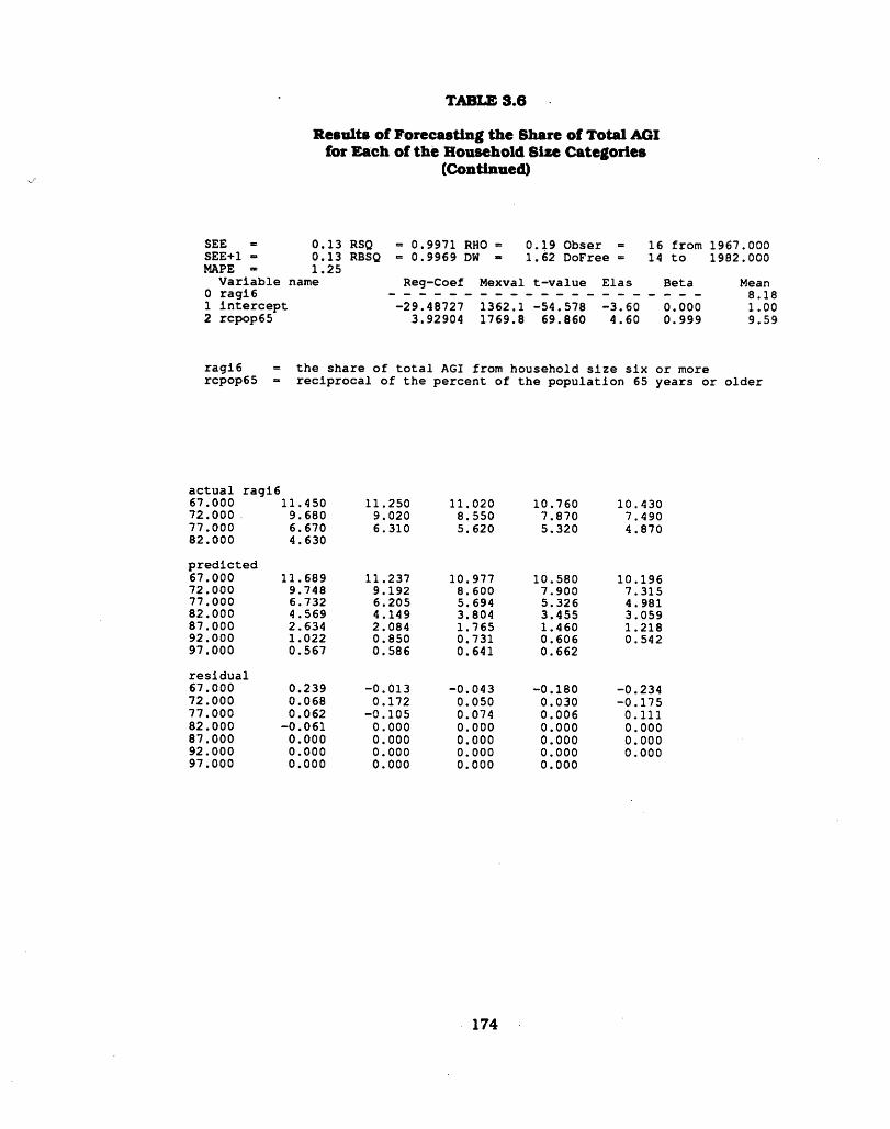
TABLE 3.6

Results of Forecasting the Share of Total AGIfor Each of the Household Size Categories

(Continued)

SEESEE+1MAPE

0.13 RSQ 0.13 RBSQ 1.25

V a r ia b le name0 ra g i€1 in te r c e p t2 rcpop65

0.9971 RHO - 0.9969 DW »

0.19 Obser 1.62 DoFree

Reg-Coef Mexval t - v a lu e E las

-29.487273.92904

16 fro m 1967.00014 to 1982.000

1362.1 -54 .578 -3 .6 0 1769.8 69.860 4.60

Beta

0.0000.999

Mean8.181.009.59

ra g i6 = th e share o f t o t a l AGI from household s iz e s ix o r more rcpop65 =* re c ip ro c a l o f th e p e rc e n t o f th e p o p u la t io n 65 years o r o ld e r

a c tu a l ra g i667.000 11.450 11.250 11.020 10.760 10.43072.000 . 9.680 9.020 8.550 7.870 7.49077.000 6.670 6.310 5.620 5.320 4.87082.000 4.630

p re d ic te d67.000 11.689 11.237 10.977 10.580 10.19672.000 9.748 9.192 8.600 7.900 7.31577.000 6.732 6.205 5.694 5.326 4 . 98182.000 4.569 4.149 3.804 3.455 3.05987.000 2.634 2.084 1.765 1.460 1.21892.000 1.022 0.850 0.731 0.606 0.54297.000 0.567 0.586 0.641 0.662

re s id u a l67.000 0.239 -0 .0 1 3 -0 .0 43 -0 .1 80 -0 .2 3472.000 0.068 0.172 0.050 0.030 -0 .1 7 577.000 0.062 -0 .1 0 5 0.074 0.006 0.11182.000 -0 .061 0.000 0.000 0.000 0.00087.000 0.000 0.000 0.000 0.000 0.00092.000 0.000 0.000 0.000 0.000 0.00097.000 0.000 0.000 0.000 0.000

174

TABLE 3.7

P opulation and Incom e D is trib u tio n By V e n tile and Household Size - 1082

E xem ptions O th e r th a n Age o r B lin d n e s s in Thousands

H ouseho ldV e n t i le

1

S iz e 1 2 3 4 5 6 T o ta l

1886.4 1249.1 1674.8 2137.4 1521 .6 2314 .1 10783.52 2426 .0 1110.9 1350.3 1750.8 154 9 .6 2 595 .9 10783.53 1365.1 1130.2 1677.1 2465.4 1828 .5 2317.1 10783.54 2363 .5 1459.7 1821.8 2066 .3 1464 .3 1608 .3 10783.85 973 .7 1458.8 1665.5 2 097 .9 1720 .5 2867.4 10783.86 2018.1 1632.2 1524.7 2319 .4 1358 .0 1931.4 10783.87 1037.8 1758.4 1609.3 2427 .3 328 2 .6 6 68 .6 10783.88 1728.3 1873.1 1746.7 1753 .9 687 .0 2 99 4 .9 10783.89 794 .7 1234 .9 1355.3 4105.4 2914 .9 3 78 .6 10783.8

10 1973.5 2513.1 2455 .9 2593 .0 688 .1 559 .8 10783.511 1494 .6 1528.3 802 .8 5172.3 959 .4 8 26 .6 10783.812 1217.1 1798.0 3092 .9 736 .3 3640 .3 299 .2 10783.813 2283 .3 2835.7 2361 .3 2138 .5 753 .2 4 11 .8 10783.714 1016.0 1329.4 1082.5 6129.6 1018 .5 208 .0 10783.815 2844 .5 2528.2 2845.7 1537 .5 762 .4 265 .2 10783.516 1367.8 3963.2 2492.3 2564 .9 354 .2 4 0 .9 10783.517 2989.8 2688 .6 3087 .6 1254.8 6 56 .6 106 .0 10783.518 3162 .7 3499.1 2186 .0 1598 .6 170 .2 1 66 .9 10783.519 3046.8 5844.3 913 .9 453 .9 255 .0 2 6 9 .6 10783.520 3 185 .6 4208.3 1320.3 1271.3 589 .1 209 .3 10783.8

T o ta ls 39175 .2 45643.5 37066.7 46574.5 26174 .2 21039 .5 215673.6

A d ju s te d G ross Income in m i l l io n s o f D o l la r s

H ouseho ldV e n t i le

1

S iz e 1 2 3 4 5 6 T o ta l

1832.4 1300.8 1351.4 1726 .9 1081.1 1755.8 9048.42 4155.2 1643.5 2196.2 2845 .8 2451 .8 4062 .0 17354.53 2 832 .6 2529.7 3709 .9 5433.7 4014 .9 5077 .5 23589 .34 6770.3 4102.6 5044.4 5748 .0 4102 .2 4406.4 30173 .95 3266.7 4901.9 5624.7 7076 .6 5789 .0 9534.0 36192 .96 7856.3 6349.5 5919.3 9066.1 5168 .0 7797 .0 42156.27 4661.5 7801.8 7175.2 10760.0 14903 .3 2874 .5 48176.38 8534.1 9320.3 8754.0 8677 .5 3410 .5 15572 .3 54268.79 4433.7 6849.4 7447.0 23327 .8 16316 .7 1992 .8 60367.4

10 11905.2 15427.8 15122.1 15320.2 4159 .0 3536 .9 65471.211 10306.1 10448.4 5364.9 36281 .3 6736.0 5611 .2 74747 .912 9135.1 13369.4 23850 .9 5297.4 26118 .4 208 7 .6 79858.813 18904.5 23620 .0 18828 .6 18465.5 6323 .0 3520 .8 89662.414 9273.3 12167.6 10205.1 54535.2 9349.3 1918 .5 97449.015 29234 .8 25610.4 27747.4 15973.0 7589.3 2531.1 108686.016 15800 .9 46263.4 29638 .8 29453 .6 4235 .8 446 .0 125838.517 38938 .8 36153 .0 38044.3 16399 .9 8229.4 1154 .7 138921.118 50420.7 53890 .9 33804 .6 24577.3 2488 .8 1818 .6 167000.919 62936.3 111019.7 18407.4 7728.7 3728 .7 6393.3 210213.520 124235.8 161632.7 45567 .6 40552.8 19007 .6 5699 .5 396696.0

T o ta ls 425434.3 554402.8 313803.8 339247.3 155202.8 87790 .5 1875881.5

175

TABLE 3.8

The D is trib u tio n o f C u to ff Per C apita AGI in C urrent D ollars fo r Selected Tears

V e n t i le 1966 1975 1982

1 4 5 5 .1 7 3 9 .6 1 212 .12 682 .4 1136 .1 1886 .43 830 .8 1443 .1 2 5 0 9 .54 9 90 .3 1780 .3 3 07 9 .05 1127 .8 2 0 8 8 .3 3 6 2 8 .86 1 283 .3 2 3 9 2 .5 4 1 6 8 .07 1415 .6 2 6 9 4 .8 4 70 4 .28 1575 .7 3 040 .3 5 3 0 1 .89 1691.4 3 322 .8 572 2 .4

10 1852 .2 3 55 3 .5 6 55 4 .511 2050 .4 4 07 0 .5 7 13 1 .212 224 6 .7 4 2 7 8 .6 7 7 6 3 .313 2483 .2 4 8 2 8 .2 8 8 8 3 .914 2 75 1 .7 5 19 6 .0 9463 .115 3014 .1 5 9 0 7 .6 11111 .616 3516.4 6769 .1 11987 .017 3 890 .6 7 816 .2 1 4253 .718 4 83 9 .6 967 2 .9 17823 .619 6 538 .3 12807 .8 2 3 1 7 1 .920 OO OO OO

176

TABLE 3.9

The D is trib u tio n o f C u to ff Per C apita AGI R elative to Average AGI fo r Selected Tears

V e n t i le 1966 1975 1982

1 18 .1 2 15.54 13 .942 2 7 .1 7 2 3 .8 7 2 1 .6 93 3 3 .0 8 3 0 .3 2 2 8 .8 54 39 .44 3 7 .4 0 3 5 .4 05 4 4 .9 1 4 3 .8 7 4 1 .7 26 5 1 .1 0 5 0 .2 6 4 7 .9 27 5 6 .3 7 5 6 .6 1 5 4 .0 88 6 2 .7 5 6 3 .87 6 0 .9 69 6 7 .3 6 69 .81 6 5 .7 9

10 7 3 .7 6 74 .65 7 5 .3 611 8 1 .6 5 85 .5 1 8 1 .9 912 8 9 .4 7 8 9 .8 8 8 9 .2 613 9 8 .8 9 101 .43 102 .1414 109 .58 109 .16 108 .8015 1 20 .03 124 .11 1 27 .7516 1 40 .03 142 .21 1 37 .8217 1 54 .93 164 .20 1 63 .8818 1 92 .73 2 03 .21 2 04 .9219 2 60 .37 2 69 .07 2 66 .4120* 2 0 .6 5 1 9 .6 9 2 1 .1 5

A ve rage AGI 2 51 1 .1 3 4760 .04 8 697 .75

*The o v e r a l l p e rc e n ta g e o f th e t o t a l incom e h e ld b y th e r ic h e s t 5% o f p o p u la t io n

177

TABLE 3.X0

Effective and Standard Tax Rates

V e n t i le 2 V e n t i le 5 V e n t i le 10

Y e a r ETR STR ETR STR ETR STR

1966 0 .4 5 0 .0 0 3 .1 9 4 .0 2 7 .1 8 8 .6 51968 0 .5 2 0 .0 0 4 .5 3 5 .8 8 8 .9 5 1 0 .6 61969 0 .6 4 0 .0 0 5 .0 3 6 .6 7 9 .5 1 1 1 .4 31970 0 .5 4 0 .0 0 4 .7 4 5 .8 1 8 .7 0 1 0 .4 61971 0 .3 5 0 .0 0 4 .0 6 4 .4 7 8 .1 0 9 .5 21972 0 .2 6 0 .1 3 3 .7 0 5 .0 9 7 .8 6 9 .5 21973 0 .4 1 0 .4 2 4 .1 9 5 .6 0 8 .4 7 10 .2 21974 0 .4 3 0 .4 9 4 .4 7 6 .0 2 8 .9 3 1 0 .7 31975 0 .0 2 0 .0 0 2 .6 3 3 .0 6 7 .8 3 9 .341976 0 .0 7 0 .0 0 3 .1 7 5 .4 5 8 .2 4 1 0 .4 61977 0 .1 6 0 .0 0 3 .1 7 2 .8 8 8 .2 9 9 .2 51978 0 .2 8 0 .0 0 3 .9 3 3 .64 8 .8 0 9 .9 31979 0 .14 0 .0 0 3 .64 3 .7 6 9 .1 0 10 .3 81980 0 .2 1 0 .0 0 4 .2 0 4 .4 6 9 .7 7 11 .341981 0 .3 4 0 .0 1 4 .6 6 5 .3 0 10 .3 1 12 .2 81982 1 .0 1 0 .0 0 4 .5 8 4 .8 1 9 .2 6 11 .2 0

V e n t i le 14 V e n t i le 17 V e n t i le 20

Y ear ETR STR ETR STR ETR STR

1966 9 .6 3 1 1 .1 5 11 .7 9 13 .20 2 0 .7 2 2 2 .6 51968 11.44 13 .1 7 13 .5 9 1 5 .2 6 2 3 .5 4 2 5 .5 01969 12 .0 9 13 .98 1 4 .2 9 16 .2 2 2 3 .9 3 2 6 .5 81970 11 .2 5 1 3 .1 5 1 3 .3 2 15 .1 0 2 2 .1 7 2 4 .9 51971 10 .64 1 2 .2 9 12 .6 6 14 .17 2 1 .4 8 2 4 .2 71972 10 .37 12 .0 0 1 2 .58 14 .1 2 2 1 .5 5 2 4 .6 51973 1 0 .9 5 12 .7 3 1 3 .1 5 14 .8 7 2 2 .0 4 2 5 .8 41974 11 .3 6 13 .2 6 1 3 .6 5 1 5 .51 2 2 .7 6 2 6 .9 11975 1 0 .6 6 12 .3 5 1 3 .3 9 15 .14 2 2 .7 5 2 7 .1 21976 10 .9 0 1 3 .0 6 1 3 .2 5 1 5 .2 6 2 3 .2 1 2 8 .0 91977 11 .07 1 2 .5 5 13 .71 1 5 .61 2 3 .9 3 2 9 .6 11978 11 .7 8 13 .67 14 .61 17 .14 2 4 .8 4 3 1 .141979 1 2 .2 2 1 4 .1 5 14 .62 16 .8 0 2 5 .5 0 3 0 .9 71980 12.64 1 4 .77 1 5 .4 9 1 8 .3 1 2 6 .3 2 3 2 .6 91981 13 .27 16 .0 7 1 5 .9 3 19 .3 8 26 .3 4 3 4 .1 31982 12 .1 8 1 4 .9 2 1 4 .5 9 1 7 .6 5 2 4 .6 0 3 1 .4 0

178

TABLE 3.11

Ratios of Effective-to-Standard Tax Rates

V e n t i le R a t io

1 *2 *3 1 .0 3 0 14 0 .9 6 9 45 0 .9 1 0 06 0 .8 6 8 77 0 .8 5 5 88 0 .8 5 6 69 0 .8 5 3 1

10 0 .8 5 2 411 0 .8 5 0 012 0 .8 4 7 413 0 .8 4 5 114 0 .8 3 9 415 0 .8 3 8 116 0 .8 3 3 417 0 .8 3 7 718 0 .8 2 9 219 0 .8 1 8 520 0 .7 7 3 8

* R a t io i s u n d e f in e d .

179

The Twelve R econcilia tion Item s vs. the NIPA Tables

TABLE 3.12

I te m T i t l e N IPA T a b le s and C o n te n ts

1 OASDI T a b le 3 .1 1 : O ld -a g e , s u r v iv o r s , and d i s a b i l i t yin s u ra n c e ( l i n e 4)

2 H I T a b le 3 .1 1 : H o s p i ta l and s u p p le m e n ta ry m e d ic a lin s u ra n c e ( l i n e 5)

3 U I T a b le 3 .1 1 : U nem ploym ent in s u ra n c e ( l i n e €)

4 RET T a b le 3 .1 1 : F e d e ra l em p loyee r e t i r e m e n t ( l i n e 1 1 ) /R a i l r o a d r e t i r e m e n t ( l i n e 1 4 ) , V e te ra n s b e n e f i t s ( l i n e 1 8 ) , B e n e f i t s fro m s o c ia l in s u ra n c e fu n d s ( l i n e 2 9 ) , E d u c a tio n ( l i n e 4 0 ) , Em ploym ent and t r a i n i n g ( l i n e 4 1 ) , and O th e r ( l i n e 42)

5 WELF T a b le 3 .1 1 : Food s tam p b e n e f i t s ( l i n e 2 2 ) , B la c k lu n gb e n e f i t s ( l i n e 2 3 ) , S u p p le m e n ta l s e c u r i t y incom e ( l i n e 2 4 ) , D i r e c t r e l i e f ( l i n e 2 5 ) , E a rn e d incom e c r e d i t ( l i n e 2 6 ) , O th e r ( l i n e 2 7 ) , and P u b l ic a s s is ta n c e ( l i n e 33)

6 O LI T a b le 8 .1 4 : O th e r la b o r incom e e x c e p t fe e s ( l i n e 4)

7 IMPU T a b le 8 .1 4 : Im p u te d incom e i n p e rs o n a l incom e ( l i n e 5)

8 VESI T a b le 8 .1 4 : In v e s tm e n t incom e o f l i f e in s u ra n c ec a r r i e r s and p r i v a t e n o n in s u re d p e n s io n p la n s ( l i n e 6 ) , In v e s tm e n t incom e r e c e iv e d b y n o n p r o f i t I n s t i t u t i o n s o r r e ta in e d b y f i d u c ia r i e s ( l i n e 7 ) , (m in u s ) T a x a b le p r i v a t e p e n s io n s ( l i n e 1 3 ) , (m in u s ) S m a ll b u s in e s s c o r p o r a t io n incom e ( l i n e 1 4 ) , and (m in u s ) O th e r ty p e s o f incom e ( l i n e 15)

9 EXCL T a b le 8 .1 4 : D i f fe r e n c e s i n a c c o u n t in g t r e a tm e n t be tw eenN IP A 's and ta x r e g u la t io n s , n e t ( l i n e 8 ) , and O th e r p e r s o n a l incom e exem pt o r e x c lu d e d fro m a d ju s te d g ro s s incom e ( l i n e 9)

P e rs o n a l c o n t r ib u t io n s f o r s o c ia l in s u ra n c e10 CONTR T a b le 8 .1 4 : P e rs o n a l( l i n e 11)

11 CAPG T a b le 8 .1 4 : N e t g a in

12 GAP T a b le 8 .1 4 : A d ju s te d

N e t g a in fro m s a le o f a s s e ts ( l i n e 12)

180

TABLE 3.13

Estimation Results for the Reconciliation Items

«1. The dependent v a r ia b le , o l i , i s o th e r la b o r income, n ic e i s t o t a l la b o r

com pensation.

SEE - 5 .25 RSQ = 0.9928 RHO - 0 .78 Obser - 28 from 1959.000SEE+1 = 3 .49 RBSQ = 0.9925 DW = 0 .45 DoFree - 26 to 1986.000MAPE = 9.95

V a r ia b le name Reg-Coef Mexval t - v a lu e E las Beta Mean0 o l i ----------------------------------------------------------------------------- 72.371 in te r c e p t -18.25168 119.5 -9 .9 6 3 -0 .2 5 0 .000 1.002 n ic e 0.08896 1077.2 59.808 1 .25 0.996 1018.66

2 . The dependent v a r ia b le , impu, i s im puted income in p e rso n a l income, p i i i s p e rs o n a l in te r e s t Income, rm otg is th e mortgage in t e r e s t r a te , and tim e is tim e tre n d v a r ia b le .

SEE - 1.51 RSQ - 0.9762 RHO = 0.14 Obser - 18 from 1966.000SEE+1 = 1.50 RBSQ = 0.9710 DW = 1.73 DoFree = 14 to 1983.000MAPE - 3.42

V a r ia b le name Reg-Coef Mexval t - v a lu e E las Beta Mean0 impu - - - - - - _ _ _ -- — - - - — - - — — - — 33.551 in te r c e p t 6.24399 14.4 2.077 0 .19 0.000 1.002 p i i 0.04043 47.6 4.065 0 .19 0.462 156.803 rm o tg [1 ] -0 .10330 0.6 -0 .3 9 6 -0 .0 3 -0 .0 2 8 8.284 tim e 1.06447 52.6 4.311 0 .65 0.566 20.50

3. The dependent v a r ia b le , v e s i, i s re ta in e d in ve s tm e n t and o th e r income, r t b i s th e th re e -m on th tre a s u ry b i l l r a te , p i i s p e rs o n a l income, and tim e is t im e tre n d v a r ia b le .

SEE = 3.67 RSQ - 0.9692 RHO - 0.30 Obser = 28 from 1959.000SEE+1 = 3 .65 RBSQ - 0.9654 DW = 1.41 DoFree - 24 to 1986.000MAPE = 19.37

V a r ia b le name Reg-Coef Mexval t - v a lu e E las Beta Mean0 v e s i - - - - - - _ _ _ .> _ _ _ _ — - - - - - - 21.611 in te r c e p t -0.28091 0 .0 -0 .1 0 9 -0 .0 1 0.000 1.002 r t b [1 ] 2.36805 45.3 5.165 0.67 0.339 6.093 P i 0.02840 156.0 11.544 1 .85 1.323 1408.404 tim e -1.75822 52.2 -5 .6 1 9 -1 .5 1 -0 .6 7 8 18.50

4. The dependent v a r ia b le , e x c l, i s o th e r ite m s w hich exempt o r exc luded from AGI. p i i s p e rso n a l Income.

SEE « 30.28 RSQ - 0.7797 RHO - 0 .79 Obser - 28 from 1959.000SEE+1 - 19.71 RBSQ - 0.7797 DW - 0 .42 DoFree = 27 to 1986.000 MAPE - 57.71

V a r ia b le name Reg-Coef Mexval t - v a lu e E las Beta Mean0 e x c l - - ----- - - - - - - - - - - - - - - ----- - 57.071 p i 0.04706 184.4 13.837 1 .16 0.712 1408.40

181

TABLE 3.13

Estimation Results for the Reconciliation Items(Continued)

5. The dependent v a r ia b le , c o n tr , i s p e rso n a l c o n t r ib u t io n f o r s o c ia l in s u ra n c e , p ic i s p r iv a te la b o r com pensation.

SEESEE+1MAPE

3.34 RSQ 2.75 RBSQ 6.09

V a r ia b le name0 c o n tr1 in te r c e p t2 p ic

0.9946 RHO 0.9944 DW

0.62 Obser = 0.77 DoFree ==

Reg-Coef Mexval t - v a lu e E las

-14.359060.08093

28 from 1959.00026 to 1986.000

156.4 -12 .037 -0 .2 6 1256.2 68.963 1 .26

Beta

0.0000.997

Mean54.431.00

849.92

6. The dependent v a r ia b le , capg, i s c a p i ta l g a in s , raaa i s th e AAA bond ra te , i n f l i s th e p e rc e n t change in th e GNP d e f la to r , and p i i s p e rs o n a l income.

SEESEE+1 - MAPE *=>

V a r ia b le name0 capg1 in te r c e p t2 ( r a a a - in f l [1 ])3 P i

14.37 RSQ 13.25 RBSQ 29.93

0.7064 RHO 0.6829 DW

0.57 Obser 0.85 DoFree

28 from 1959.000 25 to 1986.000

Reg-Coef Mexval t - v a lu e E las Beta

-9 .39706 5 .9 -1 .7 4 6 -0 .3 8 0.0001.98249 2 .1 1.040 0 .24 0.153 0.01981 40.6 4 .943 1 .14 0.729

Mean24.431.002.99

1408.40

7. The dependent v a r ia b le , gap, i s th e AGI gap. p i i s p e rso n a l income.

SEE - 6.90 RSQ « 0.9934 RHO = 0.41 Obser = 28 from 1959.000SEE+1 = 6.32 RBSQ = 0.9934 DW - 1.18 DoFree = 27 to 1986.000MAPE = 4.71

V a r ia b le name Reg-Coef Mexval t - v a lu e E las Beta MeanO s d ----------------------------------------------------------------------------- 119.301 p i 0.08535 2021.3 110.102 1.01 0.981 1408.40

182

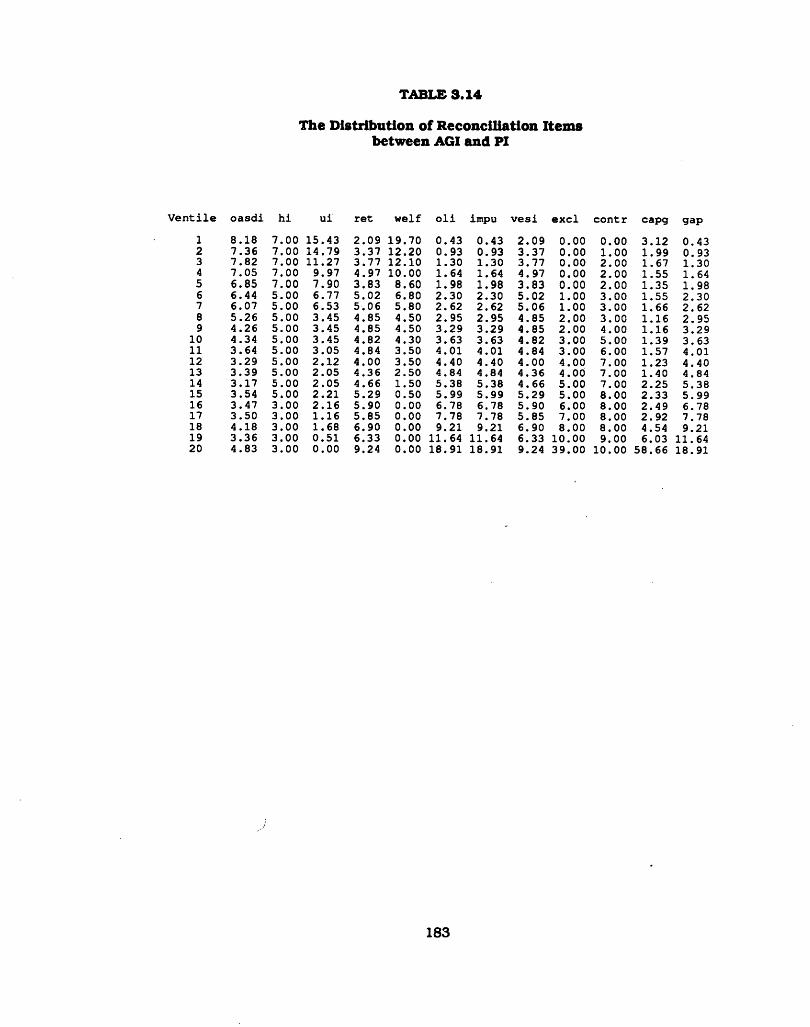
TABLE 3.14

The D is trib u tio n o f R econcilia tion Item s between AGI and PI

i t i l e oasd i h i u i re t w e lf o l i impu v e s i e x c l c o n tr capg gap

1 8 .18 7.00 15.43 2.09 19.70 0.43 0.43 2.09 0.00 0.00 3.12 0.432 7 .36 7.00 14.79 3.37 12.20 0.93 0.93 3.37 0.00 1.00 1.99 0.933 7 .82 7.00 11.27 3.77 12.10 1.30 1.30 3.77 0.00 2.00 1.67 1.304 7 .05 7.00 9.97 4.97 10.00 1.64 1.64 4.97 0.00 2.00 1.55 1.645 6 .85 7.00 7.90 3.83 8.60 1.98 1.98 3.83 0.00 2.00 1.35 1.986 6 .44 5.00 6.77 5.02 6.80 2.30 2.30 5.02 1.00 3.00 1.55 2.307 6 .07 5.00 6.53 5.06 5.80 2.62 2.62 5.06 1.00 3.00 1.66 2.628 5 .26 5.00 3.45 4.85 4.50 2.95 2.95 4.85 2.00 3.00 1.16 2.959 4 .26 5.00 3.45 4.85 4.50 3.29 3.29 4.85 2.00 4.00 1.16 3.29

10 4 .34 5.00 3.45 4.82 4.30 3.63 3.63 4.82 3.00 5.00 1.39 3.6311 3 .64 5.00 3.05 4.84 3.50 4.01 4.01 4.84 3.00 6.00 1.57 4.0112 3 .29 5.00 2.12 4.00 3.50 4.40 4.40 4.00 4.00 7.00 1.23 4.4013 3 .39 5.00 2.05 4.36 2.50 4.84 4.84 4.36 4.00 7.00 1.40 4.8414 3 .17 5.00 2.05 4.66 1.50 5.38 5.38 4. 66 5.00 7.00 2.25 5.3815 3 .54 5.00 2.21 5.29 0.50 5.99 5.99 5.29 5.00 8.00 2.33 5.9916 3 .47 3.00 2.16 5.90 0.00 6.78 6.78 5.90 6.00 8.00 2.49 6.7817 3 .50 3.00 1.16 5.85 0.00 7.78 7.78 5.85 7.00 8.00 2.92 7.7818 4 .18 3.00 1.68 6.90 0.00 9.21 9.21 6.90 8.00 8.00 4.54 9.2119 3 .36 3.00 0.51 6.33 0.00 11.64 11.64 6.33 10.00 9.00 6.03 11.6420 4 .83 3.00 0.00 9.24 0.00 18.91 18.91 9.24 39.00 10.00 58.66 18.91

183

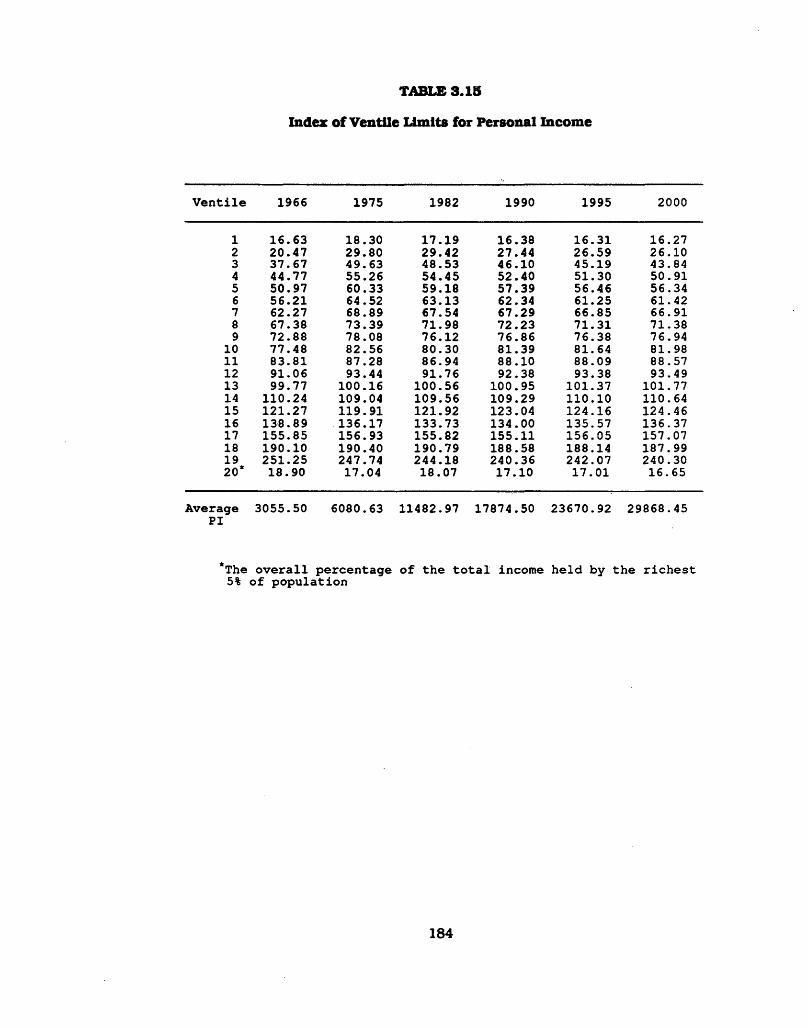
TABLE 3.15

Index of Ventile limits for Personal Income

V e n t i l e 1966 1975 1982 1990 1995 2000

1 1 6 .6 3 1 8 .3 0 1 7 .1 9 1 6 .3 8 1 6 .3 1 1 6 .2 72 2 0 .4 7 2 9 .8 0 2 9 .4 2 2 7 .4 4 2 6 .5 9 2 6 .1 03 3 7 .6 7 4 9 .6 3 4 8 .5 3 4 6 .1 0 4 5 .1 9 4 3 .8 44 4 4 .7 7 5 5 .2 6 5 4 .4 5 5 2 .4 0 5 1 .3 0 5 0 .9 15 5 0 .9 7 6 0 .3 3 5 9 .1 8 5 7 .3 9 5 6 .4 6 5 6 .3 46 5 6 .2 1 6 4 .5 2 6 3 .1 3 6 2 .3 4 6 1 .2 5 6 1 .4 27 6 2 .2 7 6 8 .8 9 6 7 .5 4 6 7 .2 9 6 6 .8 5 6 6 .9 18 6 7 .3 8 7 3 .3 9 7 1 .9 8 7 2 .2 3 7 1 .3 1 7 1 .3 89 7 2 .8 8 7 8 .0 8 7 6 .1 2 7 6 .8 6 7 6 .3 8 7 6 .9 4

10 7 7 .4 8 8 2 .5 6 8 0 .3 0 8 1 .3 9 8 1 .6 4 81 .9 811 8 3 .8 1 8 7 .2 8 8 6 .9 4 8 8 .1 0 8 8 .0 9 8 8 .5 712 9 1 .0 6 93 .4 4 9 1 .7 6 9 2 .3 8 9 3 .3 8 9 3 .4 913 9 9 .7 7 1 00 .16 1 0 0 .5 6 1 0 0 .9 5 1 0 1 .3 7 101 .7714 1 10 .24 1 09 .04 1 0 9 .5 6 1 0 9 .2 9 1 1 0 .1 0 110 .6415 1 2 1 .2 7 1 19 .91 1 2 1 .9 2 1 23 .04 1 2 4 .1 6 1 24 .4616 1 3 8 .8 9 1 36 .17 1 3 3 .7 3 1 3 4 .0 0 1 3 5 .5 7 136 .3717 1 5 5 .8 5 156 .93 1 5 5 .8 2 1 5 5 .1 1 1 5 6 .0 5 1 5 7 .0 718 1 9 0 .1 0 1 90 .40 1 9 0 .7 9 1 8 8 .5 8 1 8 8 .1 4 1 87 .9919 2 5 1 .2 5 2 4 7 .7 4 2 4 4 .1 8 2 4 0 .3 6 2 4 2 .0 7 2 4 0 .3 020* 1 8 .9 0 1 7 .0 4 1 8 .0 7 1 7 .1 0 1 7 .0 1 1 6 .6 5

A ve ra g e 305 5 .5 0 6 08 0 .6 3 11482 .97 17874 .50 2 3 6 70 .9 2 2 9 8 68 .4 5p i

*The o v e r a l l p e rc e n ta g e o f th e t o t a l Incom e h e ld b y th e r i c h e s t 5% o f p o p u la t io n

184

CHAPTER 4

TIME-SERIES CONSUMPTION FUNCTIONS

The tim e-series consum ption m odel in th is d isserta tion is an in teg ra tion o f

the previous tw o chapters. In C hapter 2, we estim ated from cross-section data the

effects o f a fam ily ’s incom e and dem ographic a ttrib u te s on household consum ption,

b u t we d id no t account fo r price effects. In the tim e series, we sha ll incorporate the

cross-section resu lts In to a system o f consum ption functions w h ich has flex ib le price

in te ractions.

To Im plem ent the PLEC in the tim e-series consum ption functions, we need

a tim e-series fo r the d is trib u tio n o f personal incom e a fte r tax. In C hapter 3, we

developed these series. W ith them and w ith tim e series on the dem ographic

variab les, we can ca lcula te how consum ption o f item i w ould have evolved over tim e

i f on ly the incom e and dem ographic effects found in the cross-section study had been

operative. T h is series we ca ll C*lt. T h is "cross-section-param eter pred ictions", C°lt,

w ill be used in the tim e-series consum ption functions to represent the effects o f

changes in incom e and dem ographic factors. Thus, C*lt conveys to the tim e series

equations w hat we learned in C hapter 2 about the effects o f changes in incom e,

incom e d is trib u tio n and dem ographic factors on consum ption.

The weighted popula tions, on the o ther hand, are used to create the

com m odity-specific, per-adu lt-equ iva lent expenditures on d iffe ren t goods. The

consum ption expenditures are estim ated and forecasted per a d u lt equivalent. To be

used in the in p u t-o u tp u t m odel, th is am ount is then m u ltip lie d by the corresponding

w eighted popula tions to obta in the aggregate consum ption. Thus, th is aggregate

to ta l is able to account fo r the s h ift in the age s tru c tu re . That is , when one

p a rtic u la r age group grows re la tive ly faste r, the consum ption demand fo r the goods

185

w hich have the m ost w eight fo r th a t group w ill grow rap id ly .

The pxlce effect in ou r tim e-series study is based on A lm on’s sym m etric

consum ption functions In "A System o f C onsum ption Functions and Its E stim ation

fo r Belgium ."1 H ie d is tin c tive feature o f A lm on’s fu n ctio n a l form Is its a b ility to

express e ithe r su b s titu tio n o r com plem entarity among goods. The m odel was

extended by Devine (1983) to allow even greater fle x ib ility In price In te ractions. O ur

tim e-series consum ption fun ctio n has the same form as th a t used In Devine (1983).

In ou r m odel, "so ft” constra in ts on the price param eters are employed to assure

reasonable estim ates.

The system o f demand equations w ill be estim ated and forecasted fo r the

aggregate expenditures on the 78 detailed com ponents o f the Personal C onsum ption

E xpenditures in the N ational Incom e and Product Accounts, w hich w ill be la te r

presented In Table 4.1. We w ill estim ate the system o f tim e-series consum ption

functions in th is chapter, and forecast each PCE com ponent in the next chapter.

I. A System o f C onsum ption Functions

A. The System

Before In troducing ou r tlm e-serles consum ption functions, we sh a ll firs t

present the no tion and the basic form o f consum ption functions in A lm on (1979).

A lm on’s system Is developed such th a t it possesses the m ain characte ristics a

consum ption fu n c tio n should have b u t was no t derived by e xp lic it u tility

m axim ization. In p a rticu la r, a consum ption fu n c tio n should have hom ogeneity o f

^ lo p p e r Almon, "A System o f Consumption Functions and its Estim ation fo r Belgium,” Southern Economic Journal 46 (July 1979) : 85 - 106.

186

degree zero In a ll prices and incom e, adding-up, and fle x ib ility in expressing price

in te ractio ns. Furtherm ore, prices should affect the budget shares and the m arg ina l

propensity to consume a p a rticu la r product. The m arg ina l propensity to consume

fo r d iffe ren t goods should be affected d iffe re n tly as incom e rises. Lastly, price

changes should affect in approxim ately equal p ropo rtion the incom e and the non­

incom e determ inants o f demand. A lthough S lu tsky sym m etry has been included in

m ost consum ption functions, it is by no means necessary fo r m arket demand

functions. However, we w ill use "approxim ate" S lu tsky sym m etry in ou r equations

to cu t down the num ber o f param eters to be estim ated.

To express the fundam ental equation fo r the dem and system , le t qi be the

q u a n tity o f consum ption on good 1; Y be incom e; Pj be the price o f good J; and P be

an index o f average prices. The demand fu n ctio n can be w ritte n as follow s:

<?t - ( Oj(f) + ) n pjv (4.1)

In E quation (4.1), the a^t) Is used to capture the effects o f a ll the non-price and non-

incom e facto rs; and a^ bt and cy are the param eters to be estim ated.

We now tu rn to the discussion o f the characte ristics and the constra in ts fo r

ou r consum ption functions represented by Equation (4.1).

1) Hom ogeneity

To guarantee the hom ogeneity o f degree zero in incom e and prices, th a t is ,

th a t m u ltip ly in g a ll the prices and incom e by a same facto r w ill lead to no changes

in the m agnitude o f consum ption expenditures, we need the fo llow ing re s tric tio n fo r

param eters c^:

187

where N Is the to ta l num ber o f goods in the system .

2) Adding-Up

Theoretica lly, we expect consum ption to exhaust incom e a t a ll prices. In

p ractice , it is d iffic u lt to b u ild the general form o f the functions w ith o u t using an

e xp lic it "spreader" to allocate the unused Income. A "spreader" can be though t o f as

a device to e lim ina te the discrepancy between Income and first-guess expenditure.

Thus, the consum ption functions should conta in a basic p a rt and a "spreader"

fu n ctio n . In the basic p a rt, both prices and incom e affect consum ption. In the

"spreader" fu n ctio n , the unused Income is allocated, in p ropo rtion to the incom e

e lastic itie s , among a ll goods to guarantee th a t the expenditures to add up to incom e.

"Spreading" is m ore desirable th a n "squeezing", w h ich scales a ll the firs t estim ates

p ropo rtion a lly to f it in to the to ta l, because it is able to p ro tect item s w ith little Income

o r price se n s itiv ity from the spreader by assigning a sm all coefficient to them . Since

spreading is no t very econom ically m eaningful, we w ill m inim ize the re liance on the

"spreader" by requ iring th a t the exhaustion o f Income be achieved a t base prices. We

w ill denote th is cond ition as "constant-price adding-up".

The "constant-price adding-up" can be represented by the fo llow ing

cond itions:

3) S lu tsky Sym m etry

S lu tsky Sym m etry states th a t the incom e-com pensated p a rtia l derivative o f

the dem and fo r good 1 w ith respect to the price o f good j is equivalent to the incom e-

com pensated p a rtia l derivative o f the demand fo r good j w ith respect to the price o f

good 1. Th is sym m etry is a property o f in d iv id u a l demand curve, b u t it is not a

property o f m arket demand curve. We show in Appendix D th a t the S lu tsky

sym m etry fo r m arket demand cannot be derived from the in d iv id u a ls ' S lutsky

equation.

In practice, the greatest advantage o f the S lu tsky sym m etry is to reduce the

num ber o f param eters to be estim ated. Thus, although the m arket demand

functions do not have th is sym m etry if in d iv id u a l consum ers have d iffe ren t shapes

o f Engel curves, we w ill use th is cond ition closely enough to help us economize on

param eters. To be more specific, we sha ll estim ate ou r equations such th a t they w ill

give th is sym m etry a t the base prices. To express th is sym m etry m athem atically, we

w ill firs t define the incom e compensated price derivative o f the demand fo r q1 w ith

respect to pj by the fo llow ing equation:

, d<3< ,(-3— ) - - i — 4.4

constant PJ

In E quation (4.4), the incom e com pensated p a rtia l derivative is derived by hold ing

rea l incom e, Y /P , constant. In effect, we have presum ed th a t P is a price index

su ffic ie n tly good th a t if Y /P is unchanged so is u tility .

G iven E quation (4.4), the S lu tsky sym m etry can be w ritte n as

fu = Ha (4.6)Sj s,

where Sj, w h ich is defined by p ^ /Y , is the budget share o f good i in a given year.

We can rew rite Equation (4.6) in a sim pler form . That is , we define a

variab le xtj by Xjj = Cy/Sj. Thus, the S lu tsky sym m etry Is represented by Ty = x^

E quation (4.1) can then be rew ritte n as

In contrast to N2 price param eters in E quation (4.1), there are only {N2-N )/2

+ N, o r (N2+N )/2 , price param eters to be estim ated in E quation (4.7). However, th is

reduction seems to be no t enough fo r our 78-equation system . There are s till too

m any param eters to be estim ated, in th is case 3081. To solve th is problem , a

grouping scheme w ill be Introduced.

B asica lly, the com m odities are grouped by th e ir characteristics in

consum ption. In our system , we com bined the 78 item s in to 10 groups. For any

com m odity i In group I and any com m odity j in group J , we assume = Tjj = X jj.

There w ill then be 45 = (102 - 10)/2 values o f xw to be estim ated. Since Xy is the

same fo r a ll com m odities i and j w ith in given I and J groups, a ll com m odities in one

group are e ithe r a ll com plem ents or a ll substitu tes fo r a ll the goods in the o ther and

a ll to the same degree. However, the com m odities in one group could be substitu tes

fo r the goods in the second group w h ile being com plem ents fo r those in some th ird .

We w ill, furtherm ore, divide each group In to subgroups to y ie ld m ore flexib le price

effects. T h is w ill be sho rtly discussed.

To form the system o f consum ption functions w ith the group s tructu re , we

w ill assume th a t the 78 com m odities are com bined in to M groups, G j through g m-

Since the value o f x is the same w ith in a p a rticu la r group, fo r any com m odity 1 in

190

j

group I and any com m odity j In group J , we m ay replace the corresponding x^’s in

E quation (4.7) w ith X ]j. Thus, to include th is group s tru c tu re . E quation (4.7) can be

re w ritte n as

„ f „ i a l y \ ®tt t i ®JT I1 r r _ SJTn r r ~ 8J X I UQt * ( clikq + b f._ ) Pi n p, ... u pj ... n pjP Je O , J JeG ,J*l J JbGu j

(4.8)

I f we define

PL = ( n Pj J r \ sL - 53 Sj (4-9)Je°L JeCL

fo r group L, and use the fo llow ing expression

Ps/T//n pljX" » _ I___ (4.10)

J e G jJ t i J p h i ' l l

fo r group I, then E quation (4.8) can be fu rth e r s im p lified as follow s:

qt - ( a ,(0 . b ~ ) n p I lX,l (411 )* L » 1

The hom ogeneity o f a consum ption fu n c tio n w ill reduce E quation (4.11) to the fin a l

form o f ou r tim e-series consum ption fu n ctio n

q, = ( a ,(fl ♦ b Z ) n ( * (e 0 , (4.12)” L=1 PL

where

PL is the specific average price o f group L; and

SL is the sum o f the budget shares o f each com m odity in group L.

N N M Msince £ Cy ■ cit + J } SjXy * ctt + £ SLxJL - stxu « 0, - stxn * - £ Sl t / l

> 1 > 1 i~ i L - l

191

In Equation (4.12), the consum ption on good 1 depends on Income, and its

re la tive prices to each o f the M groups* specific average prices, P j/P L, L = 1.....M. In

o ther w ords, the prices o f the com m odities in group L affect the demand fo r good 1

by the weighted average price index PL w ith budget shares being the w eights.

A n easy example m ay help In te rp re ting the m eaning o f the price term s in

E quation (4.12). In a tw o-group com m odity system , le t one group consist o f b u tte r

and m argarine, and the o ther conta in bread and o ther wheat products. Demand fo r

bread, therefore, depends upon Its own price and the weighted average prices o f

b u tte r and m argarine. I f m argarine accounts fo r tw o -th irds o f the to ta l expenditure

in its group, then the consum ption o f bread w ill be more s ig n ifica n tly affected by the

changes In the price o f m argarine than by the changes In the price o f b u tte r.

We w ill now Introduce the technique fo r subgroups. Suppose we have

already b u ilt 10 groups; and each o f the goods in one group is e ithe r substitu tes or

com plem ents fo r th a t in another to the same degree. We w ill ca ll th is the Inter-group

effect, and denote the price param eter fo r th is i IJt I * J . The in tra -g roup effect, on

the o ther hand, is represented by xn. To b u ild the ln tra -subgroup and the in te r­

subgroup price re la tionsh ips, we w ill need a new nota tion p. describes the price

in te ractions between subgroup S and subgroup T w ith in a p a rticu la r group.

The basic idea o f constructing subgroups w ith in each group is to yie ld a

m ore flexib le pa tte rn o f price in te ractions. The fundam ental procedure o f subgroups

is very s im ila r to the grouping scheme. The deta ils o f the deriva tion can be found in

Devine (1983). An example o f subgroups m ay be he lp fu l here. In our m odel, we

com bined the 78 com m odities In to 10 groups. The second group contains the

fo llow ing item s;

192

Group 2

a) Women’s c lo th ing

b) Men’s c lo th ing

c) Shoes and Footwear

d) Luggage

e) Jew eliy

f) T o ile t a rtic les and preparations

g) Barbershops and beauty shops

h) C leaning, laundering and shoe repa ir

We then com bined these item s In to three subgroups

Subgroup 1: C loth ing (a a n d b )

Subgroup 2: Accessories (c, d, and e)

Subgroup 3: Personal care item s (f, g, and h)

A ny com m odity in one group is e ithe r a com plem ent o r a substitu te fo r the goods in

the o ther groups to the same degree. However, a p a rticu la r subgroup m ay contain

e ithe r com plem ents o r substitu tes independently o f the o ther subgroups. Moreover,

it is possible th a t the goods in the firs t subgroup are substitu tes fo r the goods in the

second subgroup w h ile being com plem ents to the goods in the th ird . O ur resu lts w ill

show th a t Accessories Item s c, d, and e are substitu tes w ith in Subgroup 2, w hile

Personal care Item s f, g, and h are com plem ents w ith in Subgroup 3. Subgroup 2,

Accessories, are com plem ents to Subgroup 1, C loth ing, w h ile being substitu tes fo r

Subgroup 3, Personal care item s.

To see the re la tionsh ip among groups and subgroups, we show the

su b s titu tio n m atrices in Figure 4.1. T h is figu re represents a special case where

193

twelve com m odities are com bined In to three groups; and the firs t group has three

subgroups and the others have none. In the figu re , p ’s are denoted by m ’s and x's

by t ’s. The m atrices also show the p o ss ib ility th a t the goods in the firs t subgroup are

substitu tes fo r the second subgroup w h ile being com plem ents fo r the th ird . The

m 12, m 13, and 11123 param eters represent the in ter-subgroup price re la tionsh ips; and

the in tra -subgroup effects are indicated by m n , and m33.

FIGURE 4.1

The G rouping Scheme

194

B. Income and Price Elasticities

In th is section, we sh a ll derive the Income and price e lastic itie s fo r ou r tim e-

series consum ption functions. These e lastic itie s w ill be needed la te r to present ou r

estim ation resu lts .

a. Incom e E la s tic itie s

O ur Income e lastic itie s are considerably dependent upon the d is trib u tio n o f

incom e, because the incom e variab les In the tim e-series consum ption functions, C*lt ,

were derived from a non linear Engel curve (PLEC). To be m ore specific, fo r a given

good, because the slope o f each Engel curve changes from one incom e level to

another, the same am ount o f increase in Income fo r Ind iv idua ls a t d iffe ren t Income

levels w ill a ffect the changes in th e ir consum ption expenditures d iffe ren tly . In

general, we w ould expect th a t the incom e e lastic itie s o f lu xu ries are typ ica lly h igh If

the persons who were rich become even w ealth ier. On the o ther hand, the incom e

e la s tic itie s o f necessities w ould be ra th e r low fo r these people.

Since consum ption m ay be sensitive to the changes in the incom e

d is trib u tio n and to the changes in the level o f average incom e, we w ill derive

aggregate incom e e lastic itie s by fo u r d iffe ren t assum ptions. In a ll cases, aggregate

incom e increases by one percent. The firs t case assumes th a t the increase in to ta l

incom e is e n tire ly acquired by the poorest persons. In the second case, it is assumed

th a t each in d iv id u a l is given the same absolute increase in incom e. In case three,

a ll incom es are assumed to Increase by one percent. In the fo u rth case, the whole

Increase in to ta l incom e is given to the richest in d iv idua ls .

195

b. Price E lastic itie s

We w ill derive the price e lastic itie s by the usua l de fin itions. The price

e la s tic ity o f good 1 w ith respect to the price o f good J, Eg, can be w ritte n as follow s:

E« ’ ,413 )

To derive the price e lastic ities fo r our consum ption functions, we w ill firs t

take the logarithm o f E quation (4.12). The re su lt can be w ritte n as follow s:

logqt = log( at{t) + btI ) - '£ slzil < lo&Pi ~ lo&pL )F L

(4.14)

We now can derive the ow n-price and the cross-price incom e-compensated

e lastic itie s. For the ow n-price e la s tic ity o f good 1, we take the p a rtia l d iffe re n tia l o f

the (log qj) te rm w ith respect to the (log Pj) term . Th is can be done, however, more

stra igh tfo rw ard to Equation (4.8) than to Equation (4.12). From E quation (4.8), the

ow n-price e la s tic ity fo r good i is

eH - - E SLXIL * V / / (4 l5 )L»1

E quation (4.15) can be rew ritte n as

196

In E quation (4.16), the ow n-price e la s tic ity o f good 1 Is dependent upon its price

in te ractions w ith a ll the groups and subgroups weighted by the budget shares o f th a t

group o r subgroup.

For the cross-price e la s tic ity , we take the p a rtia l derivative o f (log q*) w ith

respect to (log pj) such th a t

Ey ** sj x i j (4 1 7 )

is the e la s tic ity o f demand fo r good i w ith respect to the price o f good j. Thus, the

cross-price e la s tic ity o f demand is determ ined by the price re la tionsh ip between the

tw o com m odities and the budget share o f the good whose price Is changing.

O bviously, any com m odity in group I w ill be equally affected by the changes in the

price o f good j in group J .

C. C reating "Cross-Section-Param eter P red ictions" and W eighted Populations

a. "Cross-Section-Param eter P redictions" o f C onsum ption

The "cross-section-param eter pred iction", w hich is denoted as C*It fo r good

1 and year t, w ill be used to represent the effects o f changes in income and

dem ographic facto rs. C*lt w ill show w hat w ould have happened had income and

dem ographic variab les had exactly the effects w hich the cross-section param eters

predicted. We sha ll firs t present the form ula fo r th is C*lt variab le. Let yj« be the

average am ount o f incom e received in the J1*1 income bracket in year t, D jt the

popu la tion proportion fa llin g ln to J th dem ographic category In year t, and by’s and

dy’s the estim ated cross-section param eters fo r good L Then, C*lt can be calculated

as follow s:

5 10

C 't t - b,o ♦ E b v YJ t * E * v DJ t ,4 - 181>1 >1

The variab les used to calculate the incom e com ponent o f C*lt are per capita

incom e fo r five incom e brackets, They can be viewed as being calculated by

sum m ing the am ount o f incom e over a ll ind iv idua ls in each Incom e bracket and then

d iv id ing the to ta l am ount o f incom e in th a t bracket by the popula tion. To com pute

the five Y jt’s fo r each year, the index o f d is trib u tio n o f disposable personal incom e is

used. We then assume th a t the tim e-series consum ption w ill respond to the changes

in incom e as w ould the cross-section. That is , we use the MPC’s in the cross-section,

by’s, to calculate the incom e com ponent o f th is p red iction .

The second com ponent o f the C*lt variab les is dem ographic effects. I t is

necessary to incorporate the dem ographic im pacts in the tim e-series consum ption

functions, because the cross-section resu lts show th a t they are s ig n ifica n t in

determ ining consum ption expenditures. To include the ten dem ographic effects from

the cross-section in the tim e-series analysis, the p ropo rtion o f popu la tion fa llin g in to

each o f the dem ographic categories in each year is given a w eight, dy, determ ined

from the cross-section. We d id no t include the ten dem ographic facto rs as

explanatory variables In the consum ption fu n c tio n because the p ropo rtion o f

popu la tion fo r each category changes slow ly from year to year. Even if we were to

use the ten dem ographic variab les in d iv id u a lly in the system , the degrees o f freedom

w ould be a re s tric tio n .

198

b. W eighted Populations

In the cross-section, we estim ated the a d u lt equivalency w eights fo r each o f

the 61 consum ption categories. In the tim e series, those equivalency w eights w ill be

used to construct the relevant popula tion sizes fo r d iffe ren t item s o f consum ption

expenditures. In contrast to the popula tion to ta ls , the w eighted popula tions no t on ly

account fo r the s h ift in the age s tructu re , b u t ind ica te the differences in dem and fo r

d iffe ren t com m odities by age groups. Th is difference can be illu s tra te d by g iving an

In tu itiv e exam ple. The group o f age 0 to 5 years old has highest a d u lt equivalency

w eight in W heel goods and Toys. Therefore, as the size in th is group decreases, the

w eighted popu la tion fo r toys w ill grow slow ly or decline. In the case o f m edical

expenses, longer life expectancy w ill lead to an increase in w eighted popu la tion fo r

m edical services and hea lth insurance. Figure 4.2 shows the co n trib u tio n o f the

changing age s tru c tu re o f the popula tion to the grow th o f consum ption expenditures

fo r toys and hea lth insurance.

199

FIGURE 4.2

Weighted Population

- e - TOTAL HEALTH INSURANCE -* * - TOYS

200

The C urrent Population Reports published by the Bureau o f the Census

conta ins a series o f annual estim ates o f popula tion by age2. By using these data,

we can calcula te the num ber o f people In each o f the eight age groups according to

the c lassifica tion in the cross-section. To form the com putation, le t be the

num ber o f people In age group g and year t and wlg the cross-section adu lt

equivalency w eight fo r 1th good in age group g. Thus, the weighted size o f popula tion

fo r good 1 in year t, WPit, is calculated by the fo llow ing equation:

® (4.19)WP« - £ « v t *g~ 1

Both the weighted populations and the "cross-sectlon-param eter predictions"

have to be calculated fo r each o f the 61 cross-section consum ption categories. That

is , we m ay have 61 com m odity-specific weighted populations and the C*lt’s- However,

In the tim e series we have m ore than 61 item s o f consum ption expenditures, and

some o f the tim e-series categories do no t exactly m atch the cross-section

consum ption item s. In th is case, the weighted popula tion and the C*it fo r the tim e-

series equation is calculated by using the estim ated adu lt equivalency w eights fo r the

com m odity w hich m ost closely m atches th a t o f the equation. For the item s w hich

have no correspondence in the cross-section, the single popula tion to ta l and

disposable personal Income per capita w ill be used. The deta ils o f the

correspondence between the cross-section and the tim e series sectors w ill be

represented Table 4.2.

2U.S. Bureau o f the Census, Current Population Reports. Population Estimates and Prolections. Series P-25.

D. Inco rpora ting the Cross-Section Variables

In order to make use o f the cross-section in fo rm ation in the tim e-series

dem and functions, E quation (4.12) has to be m odified to include the cross-section

Engel curve and the dem ographic variables. That is , we w ill incorporate the C*lt and

the WPit variab les in the tim e-series consum ption functions. The new equation is o f

the form

Qtt Pit ~&LXIL- ( a, + btC \t + c{AC*t( + di t ) T H g L ) w^it L r Lt

(4.20)

where

% = qua n tity o f com m odity i consumed in year t

WPlt = weighted popula tion size relevant to com m odity i in year t

C*lt = cross-section pred iction o f consum ption on good 1 in year t

t = tim e trend

plt = price o f good i in year t

PLt = average price fo r group L in year t

Sl = share in to ta l consum ption o f group L in the base period (1982)

a j, bit q , d j, xIL = param eters to be estim ated

In E quation (4.20), the C*lt and the WPlt variab les are substitu ted fo r the

incom e and the popula tion variab les used in the usual demand functions. The

advantages o f using the C*lt and the WPlt variables are notew orthy. The C*lt variab le

conta ins m ore in fo rm ation than the sim ple average o f incom e does. For instance, the

Engel curves obtained in the cross-section possess the feature th a t the m arginal

propensity to consume is d iffe ren t over d iffe ren t incom e groups by d iffe ren t

202

com m odities. F u rthe r, the dem ographic com positions o f the popula tion affect the

consum ption tendencies over tim e by the sh ifts in the proportions o f households by

region o f residence, educational achievem ent o f the household head, labor force

p a rtic ip a tio n o f spouse, household size, and age o f the household head.

The WPlt variab le, on the o ther hand, provides the in fo rm ation on the

changing d is trib u tio n o f the popula tion by using the A d u lt Equivalency W eights. As

we perceived in the cross-section analysis, d iffe ren t age groups have d iffe ren t needs

fo r d iffe ren t com m odities. The m ost s ig n ifica n t examples are the m edical expenses

and the demand fo r fu rn itu re where the form er is extrem ely high fo r the aged w hile

the la tte r is h igher fo r ch ild ren under five years. In view o f the fact th a t the

p ropo rtion o f the popula tion under five years is decreasing w h ile the elderly

popula tion over s ix ty-five years is increasing, the weighted populations are indeed

valuable fo r forecasting.

The ai(t) term in Equation (4.12) is approxim ated in E quation (4.20) by a

constant, a cyclica l variab le, and a tim e trend. The change in C*lt , AC*lt, is used to

capture the cyclica l patterns in consum ptions. The tim e trend is used to capture

secular changes in consum ption w hich were no t accounted fo r by the dem ographic

com position and the age and incom e d is trib u tio n s , such changes m ight be sh ifts in

tastes and preferences.

One o f the usual constra in ts fo r a consum ption fun ctio n is th a t the sum

across products o f income coefficients m ust be less than o r equal to 1. We w ill

im pose th is re s tric tio n on the coefficient o f ou r "incom e" variab le C*lt. That is , we

w ant to ensure the appropriate properties o f ou r consum ption fun ctio n by

constra in ing the b , param eters. The basic idea o f im posing the re s tric tio n is to

choose the coefficient such th a t e la s tic ity o f consum ption o f p roduct i w ith respect

to C*lt is equal to u n ity . Because the data used fo r estim ating the variab le C*lt d iffe r

203

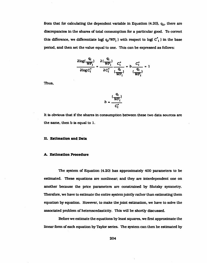
from th a t fo r ca lcu la ting the dependent variab le In Equation (4.20), qIt, there are

discrepancies in the shares o f to ta l consum ption fo r a p a rticu la r good. To correct

th is difference, we d iffe ren tia te log( q1/W P1) w ith respect to log( C*t ) In the base

period, and then set the value equal to one. T h is can be expressed as follow s:

a iog (J?L ) d ( J L )* TW y WPt C*t C\_ _ _ _ _ S _ _ _ _ _ _ _ _ _ _ _ 8 b_____

a log c*t ac* (J ? L ) ( q* ) WFt w ;

Thus,

(— ) b - J Z L

c l

I t is obvious th a t if the shares in consum ption between these two data sources are

the same, then b is equal to 1.

n . E stim a tion and Data

A . E stim a tion Procedure

The system o f Equation (4.20) has approxim ately 400 param eters to be

estim ated. These equations are non linear; and they are Interdependent one on

another because the price param eters are constrained by S lu tsky sym m etry.

Therefore, we have to estim ate the en tire system jo in tly ra th e r than estim ating them

equation by equation. However, to make the jo in t estim ation, we have to solve the

associated problem o f heteroscedastlcity. This w ill be sh o rtly discussed.

Before we estim ate the equations by least squares, we firs t approxim ate the

lin e a r form o f each equation by Taylor series. The system can then be estim ated by

204

least square m ethod and an ite ra tive procedure. H ie de ta ils o f the non linear

estim ation technique can be found in Section n.B o f C hapter 2. The same approach

w ill be applied to the tlm e-series demand equations. The ite ra tion s w ill continue

u n til the param eters w hich m inim ize the e rro r sum o f squares are obtained.

To correct heteroscedasticity, w hich vio lates the hom oscedastlcity

assum ption fo r the least squares m ethod, we w ill d ivide the data fo r each

consum ption category by an estim ate o f the standard deviation o f the disturbance

te rm in th a t equation. These estim ates are obtained by regressing the lin e a r

approxim ation form fo r each o f the 78 equations.

The size o f the cross-product o f the regressor m a trix in Equation (4.20) is

400 by 400. The least squares approach, therefore, needs to in ve rt th is huge m a trix

to generate the estim ated param eters. In our estim ation process, an a lterna tive is

adopted to make the Inversion easier, nam ely, an app lica tion o f m a trix p a rtitio n . The

inverse o f the pa rtition ed m a trix can be made by inve rting each piece o f the b lock

diagonal portions separately. Thus, the e ffo rt o f in ve rting a 400 by 400 m a trix is

avoided. It has to be m entioned, however, th a t the m a trix p a rtitio n m ethod needs

less m em ory b u t no less com putation.

B. Data

The data fo r the dependent variab le used to estim ate E quation (4.20) come

from the Personal Consum ption Expenditure (PCE) com ponent o f the N ational

Incom e and Product Accounts from 1966 to 1987. The item s o f consum ption

expenditures are reported both in cu rren t and in constant 1982 do lla rs. The data

fo r q|t is PCE in 1982 constant do lla rs. The data fo r the price variab les are obtained

by tak ing the ra tio s o f cu rre n t d o lla r PCE to constant 1982 d o lla r PCE.

205

To create the per a d u lt equivalent expenditures fo r the dependent variab les

in E quation (4.20), the PCE In 1982 do lla rs are divided by the corresponding

w eighted popula tions, WPit. The p rim ary explanatory variab les are the C*lt variables,

w hich were created by the cross-section param eters. The estim ated cross-section

param eters o f a specific com m odity should be used in con junction w ith the equations

in the tim e series w hich m ost closely m atch each other. Table 4.2 lis ts the

correspondence between the tim e-series and the cross-section sectors. I t shows from

the tab le th a t some o f the cross-section sectors are used fo r m ore than one tim e-

series sectors w h ile some o f the tim e-series sectors do no t m atch any cross-section

sectors. In th is case, a single average per capita incom e and an unw eighted

popu la tion to ta l are used fo r those w hich do no t have the corresponding sectors in

the cross-section.

206

TABLE 4.1

Tim e-Series C onsum ption Item s

1. New cars and tru cks2. Net purchases o f used cars3. New and used tru cks4. T ires and tubes5. Accessories and pa rts (auto)6. F u rn itu re , m attresses, and bedsprings7. K itchen and o ther household appliances8. C hina, glassware, tablew are, and u tensils9. Radio, IV , records, and m usical instrum ents10. F loor coverings11. D urable housefum ishings nec12. W ritin g equipm ent13. Hand too ls14. Jew elry15. O phthalm ic and orthopedic appliances16. Books and m aps17. W heel goods and durable toys18. Boats, recreationa l vehicles, and a irc ra ft19. Food, o ff prem ise20. Food, on prem ise21. A lcohol, o ff prem ise22. A lcohol, on prem ise23. Shoes and footw ear24. W omen’s c lo th ing25. Men’s clo th ing26. Luggage27. G asoline and o il28. Fuel o il and coal29. Tobacco30. Sem idurable housefum ishings31. D rug preparations and sundries32. T o ile t a rtic les and preparations33. S tationery and w ritin g supplies34. Nondurable toys and sport supplies35. Flowers, seeds, and potted p lan ts36. L igh ting supplies37. C leaning preparations38. Household paper products39. Magazines and newspaper40. O ther nondurables — id e n tity41. Owner occupied space re n t42. Tenant occupied space ren t43. H otels and m otels44. O ther housing ~ educational housing45. E le c tric ity46. N a tura l gas47. W ater and o ther san ita ry services

207

TABLE 4.1

Tim e-Series C onsum ption Item s (C ontinued)

48. Telephone and telegraph49. Dom estic services50. Household Insurance51. O ther household operations - repa ir52. Postage53. A uto repa ir54. Bridge* to lls , etc.55. A uto Insurance56. Taxicabs57. Local pub lic tran spo rt58. In te rc ity ra ilro ad59. In te rc ity buses60. A irlin e s61. Travel agents and o ther tran spo rta tio n services62. C leaning, laundering and shoe repa ir63. Barbershops and beauty shops64. Physicians65. D entists and o ther professional services66. P rivate hosp ita ls and san ita rium s67. H ealth Insurance68. Brokerage and investm ent counseling69. B ank services charges and services w ith o u t paym ent70. L ife insurance71. Legal services72. Funera l expenses and o ther personal business73. Radio and te levision repa ir74. Movies, leg itim ate theatre , and spectator sports75. O ther recreationa l services76. E ducation77. R eligious and w elfare services78. Foreign trave l

208

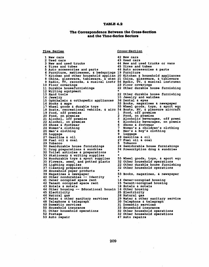
The Correspondence Between the C ross-Section and the Tim e-Series Sectors

TABLE 4.2

Time S e r ie s C ro s s -S e c t io n

1 New c a rs2 Used c a rs3 New and used t r u c k s4 T ir e s and tu b e s5 A u to a c c e s s o r ie s and p a r ts€ F u r n i t u r e , m a tt re s s e s , & b e d s p r in g s7 K itc h e n and o th e r h o u se h o ld a p p lia n8 C h in a , g la s s w a re , ta b le w a re , & u te n9 R a d io , TV, re c o rd s , & m u s ic a l i n s t r

10 F lo o r c o v e r in g s11 D u ra b le h o u s e fu rn ls h in g s12 W r i t in g equ ipm en t13 Hand t o o ls14 J e w e lry15 O p h th a lm ic & o r th o p e d ic a p p lia n c e s16 Books 6 maps17 Wheel goods & d u ra b le to y s18 B o a ts , r e c r e a t io n a l v e h ic le , & a i r c19 Food, o f f p re m ise20 Food, on p re m is e21 A lc o h o l, o f f p re m ise22 A lc o h o l, on p re m ise23 Shoes & fo o tw e a r24 Women's c lo t h in g25 M en 's c lo t h in g26 Luggage27 G a s o lin e & o i l28 F u e l o i l 6 c o a l29 Tobacco30 S e m id u ra b le house fu r n is h in g s31 D rug p re p a ra t io n s & s u n d r ie s32 T o i l e t a r t i c l e s & p re p a ra t io n s33 S ta t io n e r y & w r i t i n g s u p p lie s34 N o n d u ra b le to y s & s p o r t s u p p lie s35 F lo w e rs , seed, and p o t te d p la n ts36 L ig h t in g s u p p lie s37 C le a n in g p re p a ra t io n s38 H ouseho ld p a p e r p ro d u c ts39 M agazines & new spaper40 O th e r n o n d u ra b le s — I d e n t i t y41 Owner o c c u p ie d space r e n t42 T enan t o c c u p ie d space r e n t43 H o te ls & m o te ls44 O th e r h o u s in g — E d u c a t io n a l h o u s in45 E l e c t r i c i t y46 N a tu r a l gas47 W a te r & o th e r B a n ita r y s e rv ic e s48 T e lephone & te le g ra p h49 D om es tic s e rv ic e s50 H ouseho ld in s u ra n c e51 O th e r h o u s e h o ld o p e ra t io n s52 P ostage53 A u to r e p a i r

42 New c a rs43 Used c a rs44 New and used t r u c k s o r vans45 T ir e s and tu b e s46 A u to a c c e s s o r ie s & p a r ts19 F u r n i t u r e20 K itc h e n & h o u s e h o ld a p p lia n c e s21 C h in a , g la s s w a re , & ta b le w a re56 R a d io , TV, & m u s ic a l in s tru m e n23 F lo o r c o v e r in g s22 O th e r d u ra b le house fu r n is h in g*

22 O th e r d u ra b le house fu r n is h in g10 J e w e lry and w a tches 36 D e n ta l & eyes53 Books, m agazines 6 new spaper 55 Wheel goods, to y s , & s p o r t equ54 B o a ts , RV, & p le a s u re a i r c r a f t1 Food, o f f p re m is e2 Food, on p re m is e3 A lc o h o l ic b e v e ra g e s , o f f p re m i4 A lc o h o l ic b e v e ra g e s , on p re m ia6 Shoes & fo o tw e a r7 Women's & c h i ld r e n 's c lo t h in g8 Men ' s & b o y '8 c lo t h in g9 Luggage49 G a s o lin e & o i l27 F u e l o i l 6 c o a l5 Tobacco24 S e m id u ra b le house fu r n is h in g s34 P r e s c r ip t io n d ru g & s u n d r ie s

55 Wheel goods, to y s , & s p o r t equ 32 O th e r h o u s e h o ld o p e ra t io n s22 O th e r d u ra b le house f u r n is h in g32 O th e r h o u s e h o ld o p e ra t io n s *

53 Books, m agaz ines , 6 new spaper*14 O w n e r-o ccup ied h o u s in g15 T e n a n t-o c c u p ie d h o u s in g18 H o te ls & m o te l816 O th e r h o u s in g25 E l e c t r i c i t y26 N a tu ra l gas29 W a te r & o th e r s a n i t a r y s e rv ic e30 Te lephone & te le g ra p h31 D om estic s e rv ic e s33 H ouseho ld In s u ra n c e32 O th e r h o u s e h o ld o p e ra t io n s32 O th e r h o u s e h o ld o p e ra t io n s47 A u to r e p a ir s

209

The Correspondence Between the C ross-Section and the Tim e-Series Sectors

(C ontinued)

TABLE 4.2

Time S e r ie s C ro s s -S e c t io n

54 B r id g e , t o l l s , e t c .55 A u to in s u ra n c e56 T a x ic a b57 L o c a l p u b l ic t r a n s p o r ta t io n58 I n t e r c i t y r a i l r o a d59 I n t e r c i t y buses60 A i r l i n e s61 T ra v e l a g e n ts & o th e r t r a n s p o r t a t lo62 C le a n in g la u n d e r in g & shoe r e p a i r63 B a rbe rsh op s & b e a u ty shops64 P h y s ic ia n s65 D e n t is ts & o th e r p r o fe s s io n a l s e rv e66 P r iv a te h o s p i t a ls & s a n ita r iu m s67 H e a lth in s u ra n c e68 B ro ke ra g e & in v e s tm e n t c o u n s e lin g69 Bank s e rv ic e ch a rge s & s e rv ic e s w i t70 L i f e in s u ra n c e71 L e g a l s e rv ic e s72 F u n e ra l expenses and o th e r p e rs o n a l73 R ad io & t e le v is io n r e p a i r74 M o v ie s , le g i t im a te th e a t r e , & s p e c t75 O th e r r e c r e a t io n a l s e rv ic e s76 E d u c a tio n77 R e l ig io u s & w e lfa re s e rv ic e s78 F o re ig n t r a v e l

50 T o l ls , p a r k in g fe e s , e t c .48 A u to in s u ra n c e51 L o c a l t r a n s p o r t a t io n51 L o c a l t r a n s p o r t a t io n52 I n t e r c i t y t r a n s p o r t a t io n 52 I n t e r c i t y t r a n s p o r t a t io n 52 I n t e r c i t y t r a n s p o r t a t io n52 I n t e r c i t y t r a n s p o r t a t io n11 L a u n d r ie s & r e p a i r o f c lo t h in g13 P e rs o n a l c a re35 P h y s ic ia n s36 D e n ta l & eyes38 H o s p ita ls & s a n ita r iu m s39 H e a lth in s u ra n c e40 P e rs o n a l b u s in e s s40 P e rs o n a l b u s in e s s41 L i f e in s u ra n c e40 P e rs o n a l b u s in e s s40 P e rs o n a l b u s in e s s57 R ad io 6 TV r e p a i r s & r e n t a l58 Fees & a d m is s io n s59 O th e r r e c r e a t io n a l s u p p lie s60 E d u c a tio n61 Cash c o n t r ib u t io n

* In d ic a te s no c o rre s p o n d in g c r o s s - s e c t io n s e c to r .

m. Results

In th is section, we sha ll sum m arize the estim ation resu lts o f E quation (4.20)

by three groups o f param eters: Incom e, prices, and non-prices. Incom e e lastic itie s

are given in Table 4.3 fo r each equation. Four cases o f incom e e lastic itie s are

presented according to the fo u r d iffe ren t assum ptions about the d is trib u tio n o f the

incom e increm ent. The estim ates o f price param eters are shown in Table 4.4 by

groups and subgroups fo r own and cross price e lastic itie s. The estim ates o f non-

price param eters are given in Table 4.5. Table 4.5 also shows the m ajor s ta tis tics o f

the estim ation resu lts fo r each in d iv id u a l equation.

Ac Incom e E la s tic itie s

O ur estim ation resu lts o f incom e e lastic itie s are based on fo u r d iffe ren t

assum ptions about the d is trib u tio n o f the incom e Increm ents. There Is no unique

m easure fo r ou r Income e la s tic ity because the n on linea rity o f the Engel curve m akes

the effect o f a given increase in aggregate incom e depend upon w hich Incom e groups

receive increases. In general, we w ould expect th a t the incom e e lastic itie s o f lu xu ries

w ill be typ ica lly h igh I f hlgh-lncom e persons get the extra incom e, w h ile the incom e

e lastic itie s o f necessities w ill be re la tive ly low in th is case.

Table 4.3 shows th a t the incom e e lastic itie s o f a p a rtic u la r item are ra th e r

d iffe ren t by fo u r varying assum ptions o f the increase in incom e. The budget share

o f each item in to ta l expenditures, denoted as SHARE, is also lis te d in the table.

G enerally, the poorest people tend to increase spending on necessities as they get

be tte r o ff. For Instance, the incom e e lastic itie s o f O ff prem ise consum ption on food

and alcohol and M edical care are highest in Case 1, w hich assum es th a t the increase

211

In to ta l Income is e n tire ly acquired by the poorest persons. On the o ther hand, the

Incom e e lastic itie s o f Jew elry, Recreational expenses. In te rc ity tran spo rta tio n , and

Travel agent services are extrem ely h igh In Case 4 In w hich the richest Ind iv idua ls

are even w ealth ier.

Since there are no corresponding cross-section sectors fo r some o f the tim e-

series equations, we use a sim ple lin e a r Income variab le as a su b stitu te o f the C*it

fo r these sectors. Thus, these equations have the same value of Income e lastic itie s

across the fo u r d iffe ren t assum ptions. These equations are Indicated in Table 4.3

by an aste risk (*). We sh a ll repeat the fo u r assum ptions o f incom e increm ent as

fo llow s fo r easy reference:

CASE 1 - The one-percent Increase In to ta l Income is e n tire ly acquired by the

poorest persons.

CASE 2 - Each Ind iv idua l is given the same absolute Increase in incom e.

CASE 3 - A ll incom es increase by one percent.

CASE 4 - The one-percent Increase In to ta l Income is e n tire ly given to the

richest ind iv idua ls.

212

TABLE 4 .3

Incom e E la s tic itie s

1 NEW CARS

CASE 1

0 .4 8 3

CASE 2

2 .4 2 9

CASE 3

2 .6 6 4

CASE 4

2 .4 2 7

SHARE

3 .2 1 0

2 NET PURCHASES OF USED 2 .2 7 2 1 .4 8 6 0 .1 6 7 0 .7 5 4 1 .2 3 0

3CARSNEW AND USED TRUCKS 1 .7 0 9 2 .9 0 9 2 .3 7 5 0 .8 7 0 1 .0 2 0

4 TIRES AND TUBES 2 .1 3 9 1 .0 9 1 0 .7 6 1 0 .3 1 7 0 .6 1 0

5 ACCESSORIES AND PARTS 1 .0 8 8 1 .2 2 2 0 .9 8 0 0 .4 5 6 0 .4 8 0

6(AUTO)FURNITURE, MATTRESSES, 0 .6 0 7 1 .2 2 4 1 .5 5 7 2 .2 1 7 1 .1 5 0

7AND BEDSPRINGS KITCHEN AND OTHER 1 .4 6 8 1 .1 2 7 0 .9 3 0 0 .5 1 3 1 .0 3 0

8HOUSEHOLD APPLIANCES CHINA, GLASSWARE, 0 .9 4 3 1 .7 6 6 1 .5 6 3 0 .6 1 9 0 .5 2 0

9TABLEWARE, AND UTENSILS RADIO, TV, RECORDS, AND 2 .2 7 3 1 .1 9 3 1 .5 6 9 3 .0 2 7 2 .2 5 0

10MUSICAL INSTRUMENTS FLOOR COVERINGS 0 .5 4 6 1 .1 4 3 1 .5 5 0 2 .2 6 3 0 .4 2 0

11 DURABLE HOUSEFURNISHINGS 0 .7 8 3 1 .1 5 5 1 .4 5 3 2 .2 5 7 0 .5 2 0

12*W RITING EQUIPMENT 1 .3 0 1 1 .3 0 1 1 .3 0 1 1 .3 0 1 0 .0 5 0

13 HAND TOOLS 1 .4 3 1 2 .1 1 1 2 .6 5 5 4 .1 2 5 0 .1 7 0

14 JEWELRY 1 .0 0 1 1 .3 1 9 1 .6 5 0 2 .7 1 5 0 .9 0 0

15 OPHTHALMIC AND ORTHOPEDIC 1 .5 1 4 1 .1 3 6 1 .0 3 3 0 .9 3 9 0 .3 0 0

16APPLIANCES BOOKS AND MAPS 0 .7 2 2 0 .7 9 7 0 .7 2 6 0 .5 4 7 0 .3 2 0

17 WHEEL GOODS AND DURABLE 1 .3 2 5 1 .1 0 6 1 .2 1 3 1 .7 8 9 0 .8 6 0

18TOYSBOATS, RV, AND AIRCRAFT 1 .2 0 7 2 .3 3 4 2 .7 6 9 3 .9 6 1 0 .5 1 0

19 FOOD, OFF PREMISE 1 .2 8 5 0 .5 5 1 0 .3 9 4 0 .2 2 5 1 1 .0 7 0

20 FOOD, ON PREMISE 0 .9 2 4 1 .0 8 1 1 .1 8 2 1 .4 2 9 4 .8 5 0

21 ALCOHOL, OFF PREMISE 1 .1 8 6 0 .7 3 9 0 .6 8 4 0 .6 5 0 1 .2 5 0

22 ALCOHOL, ON PREMISE 0 .6 5 9 0 .7 4 2 0 .9 1 4 1 .3 4 9 0 .7 5 0

23 SHOES AND FOOTWEAR 1 .1 4 2 0 .9 1 5 0 .8 4 6 0 .7 0 4 0 .9 9 0

24 WOMEN'S CLOTHING 1 .0 2 4 1 .1 2 6 1 .2 5 7 1 .5 4 0 3 .5 5 0

25 MEN'S CLOTHING 0 .9 7 2 1 .1 9 0 1 .2 1 5 1 .2 0 2 1 .7 2 0

26 LUGGAGE 0 .5 3 3 1 .7 6 5 1 .9 0 1 1 .0 6 6 0 .1 0 0

27 GASOLINE AND O IL 1 .6 7 9 0 .7 7 6 0 .5 2 8 0 .2 2 8 4 .0 3 0

213

Incom e E la s tic itie s (C ontinued)

TABLE 4.3

28 FUEL O IL AND COAL

29 TOBACCO

30 SEMIDURABLE HOUSE- FURNISHINGS

31 DRUG PREPARATIONS AND SUNDRIES

3 2 *T 0 IL E T ARTICLES AND PREPARATIONS

33 *STATIONERY AND WRITING SUPPLIES

34 NONDURABLE TOYS AND SPORT SUPPLIES

35 FLOWERS, SEEDS, AND POTTED PLANTS

36 CLEANING PREPARATIONS

37 LIGHTING SUPPLIES

38 *HOUSEHOLD PAPER PRODUCTS

39 MAGAZINES AND NEWSPAPER

40*OTHER NONDURABLES — IDENTITY

41 OWNER OCCUPIED SPACE RENT

42 TENANT OCCUPIED SPACE RENT

43 HOTELS AND MOTELS

44 OTHER HOUSING — EDUCATIONAL HOUSING

45 ELECTRICITY

46 NATURAL GAS

47 WATER AND OTHER SANITARY SERVICES

48 TELEPHONE AND TELEGRAPH

49 DOMESTIC SERVICES

50 HOUSEHOLD INSURANCE

51 OTHER HOUSEHOLD OPERATIONS - REPAIR

52 POSTAGE

53 AUTO REPAIR

54 BRIDGE, TOLLS, ETC.

CASE 1 CASE 2 CASE 3 CASE 4 SHARE

1 .6 2 7 0 .6 9 0 0 .4 5 4 -0 .0 5 1 0 .8 5 0

1 .2 7 7 0 .3 1 2 0 .1 6 3 0 .0 9 2 0 .9 4 0

0 .6 6 4 1 .1 7 8 1 .1 5 0 0 .9 4 7 0 .5 2 0

1 .3 4 7 0 .8 0 2 0 .5 8 4 0 .3 1 3 0 .9 0 0

1 .9 8 2 1 .9 8 2 1 .9 8 2 1 .9 8 2 0 .8 6 0

0 .5 6 6 0 .5 6 6 0 .5 6 6 0 .5 6 6 0 .2 7 0

0 .9 8 3 0 .7 8 3 0 .8 5 8 1 .2 6 5 0 .9 0 0

0 .3 6 6 1 .7 4 6 2 .6 6 8 4 .4 9 6 0 .2 7 0

0 .3 7 6 1 .7 9 2 2 .7 3 8 4 .6 1 4 0 .1 0 0

0 .9 0 4 1 .3 3 4 1 .6 7 8 2 .6 0 7 0 .5 0 0

0 .9 3 9 0 .9 3 9 0 .9 3 9 0 .9 3 9 0 .3 7 0

0 .6 7 4 0 .7 4 4 0 .6 7 8 0 .5 1 1 0 .4 7 0

0 .0 0 0 0 .0 0 0 0 .0 0 0 0 .0 0 0 0 .1 2 0

0 .5 4 5 1 .1 5 6 1 .2 9 7 1 .5 6 1 1 0 .1 8 0

-0 .2 1 3 0 .0 6 3 0 .0 8 7 0 .1 2 7 3 .6 7 0

0 .3 1 8 1 .3 8 1 1 .5 4 5 1 .5 0 8 0 .3 7 0

0 .5 0 7 2 .4 3 4 2 .1 3 6 0 .2 5 3 0 .1 6 0

1 .4 6 5 0 .6 1 4 0 .4 7 6 0 .3 8 4 2 .1 8 0

0 .6 8 7 0 .4 3 3 0 .3 6 9 0 .3 0 0 0 .9 3 0

1 .3 4 3 0 .5 6 3 0 .4 0 5 0 .1 9 8 0 .5 5 0

0 .7 4 1 0 .4 7 9 0 .4 8 3 0 .5 3 1 1 .3 8 0

0 .4 4 3 1 .3 6 4 2 .0 1 2 3 .5 1 4 0 .3 8 0

1 .2 1 4 0 .8 1 9 0 .6 7 8 0 .4 0 5 0 .0 8 0

0 .2 3 6 1 .1 2 4 1 .7 1 8 2 .8 9 5 0 .4 3 0

0 .2 6 5 1 .2 6 4 1 .9 3 2 3 .2 5 6 0 .2 2 0

0 .9 2 2 0 .9 9 1 0 .9 7 9 1 .0 0 6 1 .8 7 0

0 .8 7 1 0 .9 9 0 0 .9 3 2 0 .7 6 6 0 .0 5 0

214

TABLE 4.3

Incom e E la s tic itie s (C ontinued)

CASE 1 CASE 2 CASE 3 CASE 4 SHARE

55 AUTO INSURANCE 1 .5 6 2 0 .9 1 3 0 .6 5 5 0 .3 7 1 0 .3 9 0

56 TAXICABS -1 .8 9 1 0 .2 5 3 0 .8 3 4 1 .6 5 5 0 .1 2 0

57 LOCAL PUBLIC TRANSPORT -2 .0 9 1 0 .2 8 0 0 .9 2 2 1 .8 2 9 0 .1 4 0

58 INTERCITY RAILROAD 0 .1 6 5 1 .0 9 2 1 .5 8 9 2 .4 4 0 0 .0 2 0

59 INTERCITY BUSES 0 .1 1 9 0 .7 8 8 1 .1 4 7 1 .7 6 2 0 .0 3 0

60 AIRLIN ES 0 .1 7 7 1 .1 6 9 1 .7 0 0 2 .6 1 2 0 .8 3 0

61 TRAVEL AGENTS AND OTHER TRANSPORTATION SERVICES

0 .1 7 2 1 .1 3 8 1 .6 5 5 2 .5 4 2 0 .0 7 0

62 CLEANING/ LAUNDERING AND SHOE REPAIR

-0 .2 5 2 0 .7 3 6 1 .0 2 6 1 .3 7 1 0 .6 1 0

63 BARBERSHOPS AND BEAUTY SHOPS

1 .2 0 9 0 .9 7 8 0 .8 4 2 0 .6 5 5 0 .6 0 0

64 PHYSICIANS 1 .2 5 5 0 .9 5 9 1 .0 0 1 1 .3 4 9 2 .5 1 0

65 DENTISTS AND OTHER PROFESSIONAL SERVICES

1 .6 0 8 1 .2 0 7 1 .0 9 7 0 .9 9 7 2 .1 0 0

66 PRIVATE HOSPITALS AND SANITARIUMS '

0 .4 9 1 0 .7 7 0 1 .6 9 6 4 .2 4 4 5 .2 5 0

67 HEALTH INSURANCE 1 .1 6 8 0 .7 1 8 0 .4 7 3 0 .2 0 7 0 .7 0 0

68 BROKERAGE AND INVESTMENT COUNSELING

1 .4 3 6 1 .5 2 8 1 .4 4 6 1 .2 2 2 0 .9 4 0

69 BANK SERVICES CHARGES AND SERVICES WITHOUT PAYMENT

1 .1 3 2 1 .2 0 4 1 .1 4 0 0 .9 6 3 2 .4 3 0

70 L IF E INSURANCE 1 .6 3 9 1 .1 4 1 1 .0 7 6 0 .9 3 3 1 .2 5 0

71 LEGAL SERVICES 1 .1 3 6 1 .2 0 9 1 .1 4 4 0 .9 6 7 0 .9 2 0

72 FUNERAL EXPENSES AND OTHER PERSONAL BUSINESS

1 .0 4 8 1 .1 1 5 1 .0 5 6 0 .8 9 2 0 .6 5 0

73 RADIO AND TELEVISION REPAIR

1 .9 2 5 0 .6 7 6 0 .4 1 5 0 .1 5 4 0 .1 1 0

74 MOVIES, LEGITIMATE THEATRE, AND SPECTATOR SPORTS

0 .7 5 9 1 .2 0 6 1 .3 5 5 1 .5 3 8 0 .5 4 0

75 OTHER RECREATIONAL SERVICES

1 .2 5 8 1 .2 0 4 1 .1 1 1 0 .8 8 1 2 .1 7 0

76 EDUCATION 1 .0 3 0 2 .3 2 6 2 .0 8 2 0 .8 4 2 1 .6 5 0

77 RELIGIOUS AND WELFARE SERVICES

1 .0 1 8 1 .2 1 3 1 .3 1 1 1 .4 2 1 2 .3 6 0

78*FOREIGN TRAVEL 2 .2 3 5 2 .2 3 5 2 .2 3 5 2 .2 3 5 0 .4 8 0

* I n d ic a te s no c o r re s p o n d in g c r o s s - s e c t io n s e c to r .

215

B. P rice E la s tic itie s

In Table 4 .4 , price e lastic itie s are presented fo r each o f the 78 tim e-series

sectors. By the grouping scheme, price re la tionsh ips among ten groups and th e ir

corresponding subgroups are also provided In the tab le . In each o f the groups, an

in d iv id u a l equation Is id e n tifie d by its equation num ber (EQ #), the subgroup It

belongs to (SUBGROUP), and its title . The estim ation resu lts fo r each item are then

lis te d in the fo llow ing o rd e r budget share (SHARE), incom e e la s tic ity (YELAS), own

price e la s tic ity (OWN), and cross price e lastic itie s (SG #1, SG #2, etc.). The title s o f

subgroups are also shown in the tab le . Incom e e lastic itie s, w hich are the resu lts o f

Case 3, are lis te d fo r the purpose o f reference. The cross price e lastic itie s m easure

the effect o f an increase in the price o f a given com m odity on the consum ption o f the

Item s in the subgroups designated by subgroup num bers.

In general, ou r estim ation resu lts o f the price param eters are satisfying .

M ost in te rp re ta tions o f the estim ates make In tu itiv e sense. The exceptions come

from the positive own price e lastic itie s fo r some Item s, a lthough these positive own

price e las tic itie s are very close to zero. To ensure the reasonableness o f our

forecasts, we sh a ll p u t the "soft" constra in t on these positive own price e lastic itie s.

T ha t is , we sh a ll force a ll positive own price e lastic itie s in ou r m odel to zero.

GROUP 1: FOOD, ALCOHOL, AND TOBACCO

The resu lts show th a t O ff and On prem ise consum ption o f food and O ff

prem ise consum ption o f alcohol have positive own price e lastic itie s . These resu lts

con trad ict one o f the properties o f the usua l demand curve th a t the norm al goods

have negative price e lastic itie s. In general, the positive cross price e lastic itie s im p ly

the su b s titu tin g w h ile the negative cross price e lastic ities ind ica te the com plem entary

216

re la tionsh ips between these tw o com m odities. For the item s w ith positive own price

e lastic itie s , the cross price e lastic itie s among them , therefore, have to be inversely

in te rp re ted . G iven the estim ated upw ard sloping dem and curves, the p rice effects

among G roup 1 can be in terpre ted as follow s: food and alcohol are com plem entary

item s fo r On prem ise consum ption; a lthough Tobacco is qu ite price in e la stic . It is a

com plem ent to the consum ption o f On prem ise alcohol and O ff prem ise food and

alcohol; and On prem ise food and alcohol are substitu tes fo r O ff prem ise food and

alcohol respectively.

GROUP 2: CLOTHING, ACCESSORIES, AND PERSONAL CARE

The own p rice e lastic itie s show th a t Women’s c lo th ing is s lig h tly price

in e la s tic (-0.977) w h ile Men’s c lo th ing is ra th e r price e lastic (-1.359) Item s. This

could be explained by the fa c t th a t women’s clo th ing is m ore fash ion oriented than

is m en’s clo th ing . Therefore, an increase in the prices o f apparel w ill s ig n ifica n tly

decrease the purchase o f m en’s c lo th ing , b u t does no t have a great im pact on the

dem and fo r women’s garm ents. The cross price e la s tic ity shows th a t these tw o item s

are substitu tes.

The own price e lastic itie s o f Accessories and Personal care item s are a ll less

than 1.0 in absolute value. Accessories and Personal care item s are com plem enting

to Apparel, a lthough the price in te ractions among three subgroups are no t

substan tia l.

GROUP 3: HOUSEHOLD DURABLES

A ll the item s in the m ajor durables subgroup are price e lastic (w ith own

price e lastic itie s between -1.598 and -1.361). B u t the item s in the m ino r durables,

whose own price e lastic itie s are on ly about -0 .5 , are price in e la stic . These resu lts

217

m igh t be explained by the fact th a t the price va ria tio n in the m ore expensive

durables Is greater than th a t In the less expensive durables, th u s the consum ption

o f the m ore costly m ajor durable item s is m ore sensitive to price changes than Is th a t

o f the m ino r durables like C hina and glassware.

The item s in the m ajor durables subgroup are substitu tes w ith one another

w ith in the same subgroup. The cross price e lastic itie s fo r those in the m ino r

durables subgroup, on the o ther hand, show th a t they are com plem ents to the o ther

Item s In the same subgroup. The resu lts also show th a t the su b s titu tio n effect

between the m ajor and the m inor durables Is very weak.

GROUP 4: HOUSEHOLD OPERATION

Except Household insurance (EQ #50, OWN = -1.015) and Postage (EQ #52,

OWN = -1.412), a ll the o ther Item s in th is group are price in e la stic . The re su lt shows

th a t the com m odities w ith in each o f the subgroups have d iffe ren t su b s titu tio n

effects. The highest su b s titu tio n effect, as expected, Is between Postage and

Telephone and telegraph. The cross price e lastic itie s among subgroups, however, are

In s ig n ifica n t.

GROUP 5: HOUSING AND HOUSEHOLD UTILm ES

The own price e lastic itie s fo r O wner-occupied space re n t and Tenant-

occupied space ren t both came ou t positive. The resu lts o f the cross price effects

show th a t O wner and Tenant occupied space ren t, as expected, are substitu tes. The

elem ents in the subgroup Household u tilitie s , in c lud ing E le c tric ity , N a tura l gas, and

Fuel o il and coal, are substitu tes w ith each o ther w ith in the subgroup.

The cross price e lastic itie s show th a t the subgroup Household u tilitie s are

com plem enting to the subgroup H ousing expenditures a lthough the price effects

218

among them are no t substan tia l.

GROUP 6: M EDICAL SERVICES

The subgroup D rugs and equipm ent is m ore price e lastic than the subgroup

Physicians and hosp ita ls. In fact, the own price e lastic itie s o f Physicians and

H ospita ls are on ly about -0 .4 . The resu lts m igh t be explained by the fa c t th a t the

need o f Physicians and H ospitals is m ore urgent th a n th a t o f D rug preparations and

O phthalm ic and orthopedic appliances in m ost cases. Therefore, Physicians and

H ospita ls w ill be less affected by th e ir own price Increases. H ie h ighest own price

e lastic itie s are in O phthalm ic and orthopedic appliances (-1.116). Thus, if there is

an overa ll increase in the prices o f m edical services, the purchase o f O phthalm ic and

orthopedic appliances is m ost lik e ly to be delayed among the m edical services.

The cross price e lastic itie s show th a t a ll the item s are substitu tes fo r the

o ther com m odities both between and w ith in subgroups.

GROUP 7: PERSONAL BUSINESS SERVICES

In general, a ll item s in th is group are price Ine lastic. Bank service charges

and services w ith o u t paym ent (EQ #69) has near zero b u t positive own price

e lastic itie s . The signs o f the cross price e lastic itie s show th a t except EQ #69, the

subgroup B anking services and the subgroup O ther personal business are

substitu tes w ith each o ther and the item s w ith in each o f the subgroups are also

substitu tes fo r the o ther item s in the same subgroup.

GROUP 8: TRANSPORTATION

The subgroup D urable purchases, in c lud ing new and used cars and tru cks ,

is a com plem ent to a ll the o ther subgroups. The item s In the subgroup M aintenance

219

expenses except gasoline and in the subgroup P ublic tran spo rta tio n are com plem ents

w ith in the same subgroup. Gasoline is a com plem ent to new and used cars w h ile

being a su b stitu te fo r the o ther tw o subgroups. That is . an increase in the price o f

gasoline w ill decrease the purchases o f new and used vehicles w h ile increasing the

expenditures on car m aintenance and pub lic transpo rta tion . T h is Increase In the

am ount spent on car m aintenance m igh t be explained by the fact th a t people w ill

postpone the purchase o f autom obiles by m a in ta in ing th e ir o ld cars when the price

o f gasoline rises.

GROUP 9: RECREATION AND TRAVEL

The own price e lastic itie s o f th is group do no t have the m agnitude we

antic ipa ted . We have expected th a t the recreationa l and tra ve l expenses are greatly

responsive to the changes In th e ir prices. The own price e lastic itie s show th a t except

M ovies, leg itim ate theatre , and spectator sports, a ll the o ther item s are price

in e la stic . In add ition , the subgroup H otels etc. has positive b u t very close to zero

own price e la s tic ity . There are alm ost no price in te ractions between hotels etc. and

the o ther three subgroups.

GROUP 10: READING AND EDUCATION

Reading and education are a ll price in e la stic item s. The cross price

e la s tic itie s show th a t reading m ateria ls are com plem ents to the o ther item s w ith in

the subgroup Reading w h ile Item s in the subgroup E ducation and re lig ious are

substitu tes. M oreover, the cross price e lastic itie s show th a t item s in these two

subgroups are substitu tes.

220

GROUP PRICE ELASTICITIES

The group price e lastic itie s m easure the in te r-g roup cross price e lastic itie s.

In the m a trix form o f group price e lastic itie s presented a t the bottom o f Table 4.4, the

effect o f price in te ractions between each p a ir o f groups are given by the average effect

over a ll the Item s In the designated groups. For exam ple, the ( ij) ^ en try o f the

m a trix Indicates the effect o f an one percent increase in the price o f an item in group

j on group L

The tab le shows th a t the pa tte rn o f price in te ractions are qu ite diverse b u t

the effects are no t s ig n ifica n t, because the grouping scheme has com bined the close

substitu tes o r com plem ents in to the same group. The su b s titu tio n o r

com plem entary re la tionsh ips between any given tw o groups are no t d ictated by any

un ifo rm param eters. Furtherm ore, they could be e ithe r substitu tes o r com plem ents

to d iffe re n t extents.

221

TABLE 4.4

Price E la s tic itie s

GROUP I s FOOD, ALCOHOL, AND TOBACCO

Q # SUBGROUP SHARE YELAS OWN SG #1 SG #2 SG #3

19 FOOD,OFF P 1 1 1 .0 7 0 .3 9 4 0 .2 4 6 - 0 . 4 4 0 - 0 . 5 8 9 0 .1 1 521 ALCOHOL,OF 1 1 .2 5 0 .6 8 4 0 .6 3 6 - 0 . 0 5 0 - 0 . 0 6 6 0 .0 1 320 FOOD,ON PR 2 4 .5 8 1 .1 8 2 0 .3 3 5 - 0 . 2 4 4 1 .4 9 4 - 0 . 0 0 422 ALCOHOL,ON 2 0 .7 5 0 .9 1 4 - 0 . 9 1 4 - 0 . 0 4 0 0 .2 4 5 - 0 . 0 0 129 TOBACCO 3 0 .9 4 0 .1 6 3 - 0 . 2 0 0 0 .0 1 0 - 0 .0 0 1 0 .0 0 0

T IT L E

EQUATION 19 FOOD, OFF PREMISE21 ALCOHOL, OFF PREMISE20 FOOD, ON PREMISE22 ALCOHOL, ON PREMISE 29 TOBACCO

SUBGROUP 1 FOOD AND ALCOHOL, OFF PREMISE2 FOOD AND ALCOHOL, ON PREMISE3 TOBACCO

GROUP 2s C LOTHING, ACCESSORIES, AND PERSONAL CARE

E £ _# SUBGROUP SHARE YELAS OWN SG #1 SG «2 SG #3

24 WOMEN'S CL 1 3 .5 5 1 .2 5 7 - 0 . 9 7 7 0 .7 4 1 - 0 . 0 0 5 - 0 . 0 1 625 M E N 'S CLOT 1 1 .7 2 1 .2 1 5 - 1 . 3 5 9 0 .3 5 9 - 0 . 0 0 3 - 0 . 0 0 823 SHOES 6 FO 2 0 .9 9 0 .8 4 6 - 0 .8 4 4 - 0 . 0 0 1 0 .0 7 0 0 .0 7 22 6 LUGGAGE 2 0 .1 0 1 .9 0 1 - 0 . 9 0 7 - 0 . 0 0 0 0 .0 0 7 0 .0 0 714 JEWELRY 2 0 .9 0 1 .6 5 0 - 0 .8 5 0 - 0 . 0 0 1 0 .0 6 3 0 .0 6 632 T O IL E T ART 3 0 .8 6 1 .9 8 2 - 0 .3 7 1 - 0 . 0 0 4 0 .0 6 3 - 0 . 2 6 963 BARBERSHOP 3 0 .6 0 0 .8 4 2 - 0 .2 9 0 - 0 . 0 0 3 0 .0 4 4 - 0 . 1 8 862 C LE A N IN G ,L 3 0 .6 1 1 .0 2 6 - 0 . 2 9 3 - 0 . 0 0 3 0 .0 4 5 - 0 . 1 9 1

T IT L E

EQUATION 24 WOMEN'S CLOTHING25 M EN 'S CLOTHING23 SHOES AND FOOTWEAR2 6 LUGGAGE14 JEWELRY32 T O IL E T A R TIC LE S AND PREPARATIONS63 BARBERSHOPS AND BEAUTY SHOPS62 C LEANING , LAUNDERING AND SHOE REPAIR

SUBGROUP 1 CLOTHING2 ACCESSORIES3 PERSONAL CARE

222

P rice E la s tic itie s (C ontinued)

TABLE 4.4

GROUP 3 : HOUSEHOLD DURABLES

EQ # SUBGROUP SHARE YELAS OWN SG #1 SG <2

6 FUR NITURE, 1 1 .1 5 1 .5 5 7 - 1 .5 7 5 0 .2 2 3 0 .0 8 37 K ITCHEN AN 1 1 .0 3 0 .9 3 0 - 1 . 5 9 8 0 .2 0 0 0 .0 7 49 R A D IO ,T V ,R 1 2 .2 5 1 .5 6 9 - 1 .3 6 1 0 .4 3 7 0 .1 6 28 C H IN A ,G LA S 2 0 .5 2 1 .5 6 3 - 0 . 5 2 8 0 .0 3 8 - 0 . 2 0 9

10 FLOOR COVE 2 0 .4 2 1 .5 5 0 - 0 . 4 8 7 0 .0 3 0 - 0 . 1 6 811 DURABLE HO 2 0 .5 2 1 .4 5 3 - 0 . 5 2 8 0 .0 3 8 - 0 . 2 0 930 SEMIDURABL 2 0 .5 2 1 .1 5 0 - 0 . 5 2 8 0 .0 3 8 - 0 . 2 0 9

T IT L E

EQUATION 6 FURNITURE, MATTRESSES, AND BEDSPRINGS7 KITCHEN AND OTHER HOUSEHOLD APPLIANCES9 R A D IO , TV , RECORDS, AND M USICAL INSTRUMENT8 C H IN A , GLASSWARE, TABLEWARE, AND U TENSILS

10 FLOOR COVERINGS11 DURABLE HOUSEFURNISHINGS NEC30 SEMIDURABLE HOUSEFURNISHINGS

SUBGROUP 1 MAJOR DURABLES2 MINOR DURABLES

GROUP HOUSEHOLD OPERATION

EQ # SUBGROUP SHARE YELAS OWN SG #1 SG * 2

3 6 CLEANING P 1 0 .1 0 2 .7 3 8 - 0 . 7 9 8 0 .1 0 7 - 0 . 0 0 23 7 L IG H T IN G S 1 0 .5 0 1 .6 7 8 - 0 . 3 7 1 0 .5 3 3 - 0 . 0 1 238 HH PAPER P 1 0 .3 7 0 .9 3 9 - 0 . 5 1 0 0 .3 9 4 - 0 . 0 0 947 WATER & OT 2 0 .5 5 0 .4 0 5 - 0 . 7 2 2 - 0 . 0 1 3 0 .3 4 349 DOMESTIC S 2 0 .3 8 2 .0 1 2 - 0 .8 2 8 - 0 . 0 0 9 0 .2 3 750 HH INSURAN 2 0 .0 8 0 .6 7 8 - 1 . 0 1 5 - 0 . 0 0 2 0 .0 5 051 OTHER HOUS 2 0 .4 3 1 .7 1 8 - 0 . 7 9 6 - 0 . 0 1 0 0 .2 6 873 RADIO & TE 2 0 .1 1 0 .4 1 5 - 0 . 9 9 6 - 0 . 0 0 3 0 .0 6 952 POSTAGE 3 0 .2 2 1 .9 3 2 - 1 .4 1 2 0 .0 5 2 0 .0 8 248 TELEPHONE 3 1 .3 8 0 .4 8 3 - 0 . 5 0 6 0 .3 2 5 0 .5 1 3

T IT L E

EQUATION 36 CLEANING PREPARATIONS37 L IG H T IN G SUPPLIES38 HOUSEHOLD PAPER PRODUCTS47 WATER AND OTHER SANITARY SERVICES49 DOMESTIC SERVICES50 HOUSEHOLD INSURANCE51 OTHER HOUSEHOLD OPERATIONS — R EPAIR 73 RADIO AND T E LE V IS IO N REPAIR52 POSTAGE48 TELEPHONE AND TELEGRAPH

SUBGROUP 1 CLEANING AND PAPER PRODUCTS2 SERVICES AND INSURANCE3 COMMUNICATION

SG «3

0 .0 2 40 .1 1 80 .0 8 70 .2 0 50 .1 4 10 .0 3 00 .1 6 00 .0 4 10 .1 7 21 .0 7 8

223

TABLE 4.4

Price E la s tic itie s (C ontinued)

GROUP 5 : HOUSING AND HOUSEHOLD U T IL IT IE S

EQ # SUBGROUP SHARE YELAS OWN SG #1 SG #2

41 OWNER OCCU 1 1 0 .1 8 1 .2 9 7 1 .2 1 0 - 2 . 3 5 0 0 .2 8 342 TENANT OCC 1 3 .6 7 0 .0 8 7 2 .7 1 3 - 0 . 8 4 7 0 .1 0 245 E L E C T R IC IT 2 2 .1 8 0 .4 7 6 - 0 . 0 5 7 0 .0 6 1 0 .1 7 746 NATURAL GA 2 0 .9 3 0 .3 6 9 - 0 . 1 5 9 0 .0 2 6 0 .0 7 628 FUEL O IL & 2 0 .8 5 0 .4 5 4 - 0 . 1 6 5 0 .0 2 4 0 .0 6 9

T IT L E

EQUATION 41 OWNER OCCUPIED SPACE RENT42 TENANT OCCUPIED SPACE RENT45 E LE C T R IC IT Y46 NATURAL GAS28 FUEL O IL AND COAL

SUBGROUP 1 HOUSING2 HOUSEHOLD U T IL IT IE S

GROUP 6 : MEDICAL SERVICES

EQ # SUBGROUP SHARE YELAS OWN SG #1 SG #2

64 P H Y S IC IA N S 1 2 .5 1 1 .0 0 1 - 0 . 4 0 9 0 .1 0 2 0 .2 2 365 D EN TISTS fi 1 2 .1 0 1 .0 9 7 - 0 . 4 2 6 0 .0 8 6 0 .1 8 766 P R IVA TE HO 1 5 .2 5 1 .6 9 6 - 0 . 2 9 7 0 .2 1 4 0 .4 6 667 HEALTH IN S 1 0 .7 0 0 .4 7 3 - 0 . 4 8 3 0 .0 2 9 0 .0 6 215 OPHTHALMIC 2 0 .3 0 1 .0 3 3 - 1 . 1 1 6 0 .0 2 7 0 .0 6 831 DRUG PREPA 2 0 . 90 0 .5 8 4 - 0 . 9 8 0 0 .0 8 0 0 .2 0 3

T IT L E

EQUATION 64 P H Y S IC IA N S65 D ENTISTS AND OTHER PROFESSIONAL SERVICES66 P R IVA TE HOSPITALS AND SANITARIUM S67 HEALTH INSURANCE15 OPHTHALMIC AND ORTHOPEDIC APPLIANCES31 DRUG PREPARATIONS AND SUNDRIES

SUBGROUP 1 P H Y S IC IA N S AND HOSPITALS2 DRUGS AND EQUIPMENT

224

TABLE 4.4

Price E la s tic itie s (C ontinued)

GROUP 7 : PERSONAL BUSINESS SERVICES

& _ # SUBGROUP SHARE YELAS OWN SG #1 SG #2

68 BROKERAGE 1 0 .9 4 1 .4 4 6 - 0 . 2 5 8 0 .1 7 9 0 .0 1 169 BANK SER VI 1 2 .4 3 1 .1 4 0 0 .0 2 6 0 .4 6 3 0 .0 2 970 L IF E INSUR 2 1 .2 5 1 .0 7 6 - 0 . 1 6 6 0 .0 1 5 0 .2 9 071 LEGAL SERV 2 0 .9 2 1 .1 4 4 - 0 . 2 4 3 0 .0 1 1 0 .2 1 372 FUNERAL EX 2 0 .6 5 1 .0 5 6 - 0 . 3 0 5 0 .0 0 8 0 .1 5 1

T IT L E

EQUATION 68 BROKERAGE AND INVESTMENT COUNSELING69 BANK SERVICE CHARGES AND SERVICES WITHOUT PAYMENT70 L IF E INSURANCE71 LEGAL SERVICES72 FUNERAL EXPENSES AND OTHER PERSONAL BUSINESS

SUBGROUP BANKING SERVICES OTHER PERSONAL BUSINESS

GROUP 8 : TRANSPORTATION

EQ § SUBGROUP SHARE YELAS OWN SG #1 SG #2 SG #3 SG #4

1 NEW CARS 1 3 .2 1 2 .6 6 4 - 0 . 0 3 1 0 .4 1 0 - 0 . 1 9 7 - 1 . 1 4 8 - 0 . 0 8 52 USED CARS 1 1 .2 3 1 .1 6 7 - 0 .2 8 4 0 .1 5 7 - 0 . 0 7 6 - 0 . 4 4 0 - 0 . 0 3 33 TRUCKS 1 1 .0 2 2 .3 7 5 - 0 .3 1 1 0 .1 3 0 - 0 . 0 6 3 - 0 . 3 6 5 - 0 . 0 2 74 T IR E S & TU 2 0 .6 1 0 .7 6 1 - 0 . 0 6 8 - 0 . 0 3 8 - 0 . 0 0 2 0 .4 3 5 0 .0 1 15 ACCESSORIE 2 0 .4 8 0 .9 8 0 - 0 . 0 6 7 - 0 . 0 3 0 - 0 . 0 0 1 0 .3 4 2 0 .0 0 9

53 AUTO R E PA I 2 1 .8 7 0 .9 7 9 - 0 . 0 7 2 - 0 . 1 1 5 - 0 . 0 0 6 1 .3 3 4 0 .0 3 555 AUTO INSUR 2 0 .3 9 0 .6 5 5 - 0 . 0 6 7 - 0 . 0 2 4 - 0 . 0 0 1 0 .2 7 8 0 .0 0 754 B R ID G E ,T O L 2 0 .0 5 0 .9 3 2 - 0 . 0 6 6 - 0 . 0 0 3 - 0 . 0 0 0 0 .0 3 6 0 .0 0 156 TAXICABS 3 0 .1 2 0 .8 3 4 - 0 . 3 9 0 - 0 . 0 4 3 0 .0 8 6 - 0 . 2 8 1 0 .0 0 25 7 LOCAL PUBL 3 0 .1 4 0 .9 2 2 - 0 . 4 3 7 - 0 . 0 5 0 0 .1 0 0 - 0 . 3 2 8 0 .0 0 327 GASOLINE & 4 4 .0 3 0 .5 2 8 - 0 . 0 7 7 - 0 . 1 0 7 0 .0 7 6 0 .0 8 1 0 .0 0 0

T IT L E

EQUATION

SUBGROUP

1 NEW CARS2 NET PURCHASES OF USED CARS3 TRUCKS4 T IR E S AND TUBES5 ACCESSORIES AND PARTS (AUTO)

53 AUTO REPAIR55 AUTO INSURANCE54 B R ID G E, TO LLS, ETC5 6 TAXICABS57 LOCAL P U B L IC TRANSPORT27 GASOLINE AND O IL

1 DURABLE PURCHASES2 MAINTENANCE EXPENSES EXCEPT GASOLINE3 P U B L IC TRANSPORTATION4 GASOLINE

225

TABLE 4.4

Price E la s tic itie s (C ontinued)

GROUP 9 : RECREATION AND TRAVEL

EQ # SUBGROUP SHARE YELAS OWN SG #1 SG #2 SG #3 SG * 4

74 M O V IE S ,LE G 1 0 .5 4 1 .3 5 5 - 1 . 7 6 7 0 .3 7 8 - 0 . 0 1 0 0 .1 9 7 0 .0 0 075 OTHER RECR 1 2 .1 7 1 .1 1 1 - 0 . 6 2 5 1 .5 2 1 - 0 . 0 4 1 0 .7 9 3 0 .0 0 118 BOATS,RECR 2 0 .5 1 2 .7 6 9 - 0 . 8 1 6 - 0 . 0 1 0 0 .2 1 1 - 0 . 0 0 8 - 0 . 0 0 017 WHEEL GOOD 2 0 .8 6 1 .2 1 3 - 0 . 6 7 1 - 0 . 0 1 6 0 .3 5 5 - 0 . 0 1 3 - 0 . 0 0 034 NONDURABLE 2 0 .9 0 0 .8 5 6 - 0 . 6 5 4 - 0 . 0 1 7 0 .3 7 2 - 0 . 0 1 4 - 0 . 0 0 035 FLOWERS, SE 2 0 .2 7 2 .6 6 8 - 0 . 9 1 5 - 0 . 0 0 5 0 .1 1 1 - 0 . 0 0 4 - 0 . 0 0 013 HAND TOOLS 2 0 .1 7 2 .6 5 5 - 0 . 9 5 6 - 0 . 0 0 3 0 .0 7 0 - 0 . 0 0 3 - 0 . 0 0 058 R A IL R O A D ,I 3 0 .0 2 1 .5 8 9 - 0 . 9 3 6 0 .0 0 7 - 0 . 0 0 0 0 .0 0 1 - 0 . 0 0 05 9 B U S E S ,IN T E 3 0 .0 3 1 .1 4 7 - 0 . 9 3 6 0 .0 1 1 - 0 . 0 0 0 0 .0 0 1 - 0 .0 0 160 A IR L IN E S 3 0 .8 3 1 .7 0 0 - 0 . 9 0 2 0 .3 0 3 - 0 . 0 1 3 0 .0 3 5 - 0 . 0 1 961 TRAVEL AGE 4 0 .0 7 1 .6 5 5 0 .0 3 9 0 .0 0 0 - 0 . 0 0 0 - 0 . 0 0 2 0 .0 0 178 FOREIGN TR 4 0 .4 8 2 .2 3 5 0 .0 4 3 0 .0 0 0 - 0 . 0 0 0 - 0 . 0 1 1 0 .0 0 543 HOTELS & M 4 0 .3 7 1 .5 4 5 0 .0 4 2 0 .0 0 0 - 0 . 0 0 0 - 0 . 0 0 9 0 .0 0 4

T IT L E

EQUATION 74 M O VIES, LE G IT IM A T E THEATRE, SPECTATOR SPORTS75 OTHER RECREATIONAL SERVICES18 BOATS, RECREATIONAL V E H IC LE S , AND AIRCRAFT17 WHEEL GOODS AND DURABLE TOYS34 NONDURABLE TOYS AND SPORT SUPPLIES35 FLOWERS, SEEDS, AND POTTED PLANTS13 HAND TOOLS58 IN T E R C IT Y RAILROAD5 9 IN T E R C IT Y BUSES60 A IR L IN E S61 TRAVEL AGENTS AND OTHER TRANSPORTATION SERVICES 78 FOREIGN TRAVEL43 HOTELS AND MOTELS

SUBGROUP 1 ADM ISSIONS2 RECREATIONAL NONDURABLES AND DURABLE3 TRAVEL EXPENSES4 HOTELS ETC.

226

TABLE 4.4

P rice E la s tic itie s (C ontinued)

GROUP 1 0 : READING AND EDUCATION

EQ i SUBGROUP SHARE YELAS OWN SG #1 SG »2

16 BOOKS & MA 1 0 .3 2 0 .7 2 6 - 0 . 5 6 6 - 0 . 2 9 5 0 .1 0 939 MAGAZINES 1 0 .4 7 0 .6 7 8 - 0 . 7 0 5 - 0 . 4 3 4 0 .1 5 912 W R IT IN G EQ 1 0 .0 5 1 .3 0 1 - 0 . 3 1 7 - 0 . 0 4 6 0 .0 1 733 STATIONERY 1 0 .2 7 0 .5 6 6 - 0 . 5 2 0 - 0 . 2 4 9 0 .0 9 276 EDUCATION 2 1 .6 5 2 .0 8 2 - 0 .4 8 1 0 .5 6 0 0 .1 4 377 R E LIG IO U S 2 2 .3 6 1 .3 1 1 - 0 . 4 2 0 0 .8 0 1 0 .2 0 544 OTHER HOUS 2 0 .1 6 2 .1 3 6 - 0 . 6 1 1 0 .0 5 4 0 .0 1 4

T IT L E

EQUATION 16 BOOKS AND MAPS39 MAGAZINES AND NEWSPAPER12 W R ITIN G EQUIPMENT33 STATIONERY AND W R ITIN G SUPPLIES76 EDUCATION77 R E LIG IO U S AND WELFARE SERVICES44 OTHER HOUSING — EDUCATIONAL HOUSING

SUBGROUP 1 READING2 EDUCATION AND R E LIG IO U S

= === '

GROUP PR IC E E L A S T IC IT IE S

GROUP 1 2 3 4 5 6 7 8 9 10

1 0 .,0 0 0 - 0 . 0 0 1 - 0 . 0 0 0 0 .0 1 7 0 .0 0 5 - 0 . 0 4 2 - 0 . 0 1 3 0 .0 2 5 - 0 . 0 0 0 - 0 . 0 0 92 - 0 . ,0 0 2 0 .0 0 0 0 .0 4 5 - 0 .0 2 8 0 .1 5 6 0 .0 4 5 - 0 . 0 2 2 - 0 . 0 0 7 - 0 . 0 0 3 - 0 . 0 3 23 - 0 . ,00 1 0 .0 5 7 0 .0 0 0 0 .0 0 1 0 .3 4 9 - 0 . 1 3 9 - 0 . 0 3 3 - 0 . 0 5 8 - 0 . 0 0 2 0 .0 3 64 0 .,1 4 9 - 0 . 0 7 9 0 .0 0 2 0 .0 0 0 - 0 . 2 8 7 0 .0 7 6 0 .0 1 4 0 .0 7 9 0 .0 0 2 - 0 . 0 8 55 0 . 00 5 0 .0 5 1 0 .0 9 0 - 0 .0 3 3 0 .0 0 0 - 0 . 0 8 0 - 0 . 0 3 8 - 0 . 0 3 1 - 0 . 0 0 1 - 0 . 0 2 66 - 0 . ,0 8 0 0 .0 2 7 - 0 . 0 6 5 0 .0 1 5 - 0 . 1 4 5 0 .0 0 0 0 .0 6 4 0 .0 2 3 0 .0 0 1 0 .0 8 47 - 0 . ,0 3 9 - 0 . 0 2 1 - 0 . 0 2 5 0 .0 0 5 - 0 . 1 1 0 0 .1 0 2 0 .0 0 0 0 .0 1 5 - 0 . 0 0 0 0 .0 0 48 0 . 07 9 - 0 . 0 0 7 - 0 . 0 4 5 0 .0 2 7 - 0 .0 9 4 0 .0 3 8 0 .0 1 6 0 .0 0 0 0 .0 0 3 - 0 . 0 0 39 - 0 . 001 - 0 . 0 0 6 - 0 . 0 0 2 0 .0 0 2 - 0 . 0 0 3 0 .0 0 2 - 0 . 0 0 0 0 .0 0 5 0 .0 0 0 - 0 .0 0 4

10 - 0 . 044 - 0 . 0 5 0 0 .0 4 4 - 0 . 0 4 6 - 0 .1 2 1 0 .2 1 9 0 .0 0 6 - 0 . 0 0 4 - 0 . 0 0 3 0 .0 0 0

T IT L E

GROUP 1 FOOD, ALCOHOL, & TOBACCO2 CLO THING , ACCESSORIES, & PERSONAL CARE3 HOUSEHOLD DURABLE4 HOUSEHOLD OPERATION5 HOUSING & HOUSEHOLD U T IL IT IE S6 M EDICAL SERVICES7 PERSONAL BUSINESS SERVICES8 TRANSPORTATION9 RECREATION AND TRAVEL

10 READING AND EDUCATION

227

C. Estimates of Non-Price Parameters

Table 4.5 provides the resu lts o f the estim ated non-price param eters in

E quation (4.20). We sha ll repeat th is equation fo r easy reference:

J “ - = ( a, + b ,c '„ ♦ c ,a c *(4 + d , t ) m f ! ! )-**•’ «• w rtt l i'u

The param eter in colum n A is the constant term . The param eter in colum n

B is constrained and is equal to the ra tio o f ( q j/W P j) to C*j in E quation (4.20). The

param eter in colum n C is the effect o f the firs t difference o f C*t on consum ption

expenditures. In other words, it m easures the im pact o f the cyclica l changes in the

economy on a consum ption item . The param eter in colum n D m easures the effect

o f tim e trend , w hich accounts fo r the im pact o f the factors o ther than incom e, price,

and dem ographic variab les on the am ount o f expenses o f a given com m odity. The

param eter in colum n E is the coefficient o f the equation-specific variables, w hich w ill

be sho rtly discussed. The regression s ta tis tics fo r each o f the equations include

m ean absolute percentage e rro r (MAPE) and R2. E rro r sum o f squares (ESS) are also

lis te d fo r each equation.

We have used add itiona l variables in a lin e a r form w h ile estim ating E quation

(4.20) fo r some o f the sectors. The extra variab les and the corresponding equations

using those variab les are as follow s:

a. A dum m y variab le fo r n a tu ra l gas supply constra in ts

The dum m y variab le is given a value o f one during the period 1974, 1975,

and 1976 where gas was in short supply due to price regu la tion and zero otherw ise.

The variab le Is used in sector 28 o f Fuel o il and coal, sector 45 o f E le c tric ity , and

228

sector 46 o f N a tura l gas. H ie resu lts show th a t th is variab le has negative im pact on

E le c tric ity and N a tura l gas b u t has very little effect on Fuel o il and coal.

b . A proxy fo r the po ten tia l stock o f cars fo r the use-car m arket

T h is variab le is used in sector 2 fo r the Used cars equation. I t is calculated

by a three year m oving average o f new car purchases lagged three years.

c. The m o rta lity ra te

The m o rta lity ra te is Included in equation 72, Funeral expenses and other

personal business, to capture the negative im pact o f the Increasing longevity.

d. A proxy fo r the speculative demand fo r housing

T h is variab le is com puted as a ra tio o f M2 m oney supply to GNP. It is

included in housing sector 41 o f Owner occupied space ren t and sector 42 o f Tenant

occupied space ren t.

e. The sho rt term bond rate

This variab le is used in the fo llow ing cyclica l sectors: sector 1 o f New cars,

sector 3 o f New and used trucks, and sector 18 o f Boats, recreationa l vehicle, and

a irc ra ft. I t is m easured by the 4-6 m onth com m ercial paper rate .

229

f. A tim e trend variab le fo r the taste changes In alcohol consum ption and

the changes In the demand fo r pub lic transporta tion

In equations 21 and 22, a tim e trend s ta rtin g w ith the value one is Imposed

on period 1980 through the rest o f the periods to capture the taste changes in the

o ff and the on prem ise consum ption o f alcohol. I t is also used in equation 57 o f

Local p u b lic transpo rta tion and equation 58 o f In te rc ity ra ilro ad to capture the

downward trend o f consum ption in these two sectors.

230

TABLE 4.5

Estim ates o f Non-Price Param eters

GROUP 1 : FOOD, ALCOHOL,

1 2 SG A

19 FOOD,OFF P 1 - 1 4 3 .3 3 121 ALCOHOL, OF 1 - 3 3 8 .7 4 720 FOOD,ON PR 2 8 4 .0 7 122 ALCOHOL, ON 2 4 5 0 .1 6 729 TOBACCO 3 8 8 .0 8 8

: TOBACCO

B c D E

0 .6 6 2 1..7 2 9 2 .0 9 61 .2 3 3 - 0 . .7 5 5 4 .6 4 9 - 8 . 0 1 80 .7 5 4 - 0 . .3 6 9 - 0 . 9 3 20 .7 8 3 - 0 . .3 7 4 - 5 . 3 6 1 2 .3 4 20 .9 1 6 0..4 9 2 - 0 . 8 9 6

MAPE RSQ ESS SHARE

4 .1% - 1 . 0 3 1 6 1 8 2 1 . 1 1 .11 .7 % 0 .9 3 3 5 1 4 . 1 .22 .0% 0 .9 6 2 2 1 2 3 . 4 .62 .0% 0 .4 8 8 2 2 5 . 0 .71 .5% 0 .8 7 1 1 8 4 . 0 .9

T IT L E

EQUATION 1 9 FOOD, OFF PREMISE21 ALCOHOL, OFF PREMISE 20 FOOD, ON PREMISE22 ALCOHOL, ON PREMISE 2 9 TOBACCO

GROUP 2 : C LOTHING, ACCESSORIES, & PERSONAL CARE

m SG A B C D E MAPE RSQ ESS SHARE

24 WOMEN'S CL 1 - 4 1 .4 4 8 1 .1 5 6 - 0 . 2 5 9 0 .3 5 6 1 .9% 0 .9 9 3 6 5 5 . 3 .525 M EN 'S CLOT 1 - 4 . 0 2 8 1 .0 8 9 - 0 . 3 8 8 0 .0 4 9 1 .4% 0 .9 9 1 1 2 1 . 1 .723 SHOES £ FO 2 6 0 .5 2 5 1 .2 6 5 - 0 . 7 2 7 - 0 . 7 8 2 2 .5 % 0 .9 5 9 1 4 9 . 1 .026 LUGGAGE 2 9 .0 5 7 1 .9 2 2 - 0 . 8 1 2 - 0 . 1 1 9 3 .4% 0 .9 1 8 3 . 0 .114 JEWELRY 2 - 5 2 .5 9 3 1 .4 9 7 - 0 . 9 1 2 0 .6 0 5 5 .8 % 0 .9 5 5 4 7 0 . 0 .932 T O IL E T ART 3 3 1 .0 9 8 1 .6 4 4 - 1 . 0 2 0 - 1 . 3 6 1 1 .9% 0 .9 2 2 6 7 . 0 .963 BARBERSHOP 3 6 1 .1 0 5 0 .5 5 4 0 .2 1 6 - 0 . 7 3 6 5 .2 % 0 .3 8 9 2 1 2 . 0 .662 C L E A N IN G ,L 3 1 6 4 .8 6 5 1 .3 2 5 0 .0 9 6 - 1 .9 8 1 6.2% 0 .6 1 3 6 3 2 . 0 .6

T IT L E

EQUATION 24 WOMEN'S CLOTHING25 M EN 'S CLOTHING23 SHOES AND FOOTWEAR26 LUGGAGE14 JEWELRY32 T O ILE T A R TIC LE S AND PREPARATIONS63 BARBERSHOPS AND BEAUTY SHOPS62 CLEANING , LAUNDERING AND SHOE REPAIR

231

TABLE 4.5

Estimates of Non-Price Parameters(Continued)

GROUP 3 : HOUSEHOLD DURABLES

E & SG A B C D E MAPE ESS SHARE

6 FU RN ITUR E, 1 - 9 1 .4 6 9 0 .5 8 4 - 0 . 3 7 2 1 .2 8 1 3 .1% 0 .8 9 3 8 7 7 . 1 .17 KITC HEN & 1 - 5 7 .4 4 6 1 .0 1 3 - 0 . 1 1 9 0 .5 9 2 3 .6% 0 .9 4 9 2 0 0 . 1 .09 R A D IO ,T V ,R 1 - 1 8 .8 4 0 1 .6 3 5 - 0 . 5 3 6 - 0 . 5 7 5 7 .3% 0 .9 8 9 1 0 9 5 . 2 .28 C H IN A ,G LA S 2 1 1 6 .2 4 0 2 .7 9 0 - 1 . 8 2 8 - 1 . 4 1 2 3 .0% 0 .4 2 0 3 5 9 . 0 .5

10 FLOOR,COVE 2 - 9 . 4 5 5 1 .2 3 5 - 0 . 9 9 1 0 .1 2 5 5 .6% 0 .8 7 6 7 0 . 0 .411 DURABLE HO 2 - 3 3 .8 3 3 0 .5 3 4 - 0 .3 4 8 0 .4 3 2 3 .9% 0 .9 4 5 1 3 9 . 0 .530 SEMIDURABL 2 5 0 .9 1 6 0 .8 2 7 - 0 . 6 2 7 - 0 . 5 7 6 2 .8 % - 0 . 5 0 1 1 0 6 . 0 .5

T IT L E

EQUATION 6 FURNITURE, MATTRESSES, AND BEDSPRINGS7 KITCHEN AND OTHER HOUSEHOLD APPLIANCES9 R A D IO , TV , RECORDS, AND M USICAL INSTRUMENT8 C H IN A , GLASSWARE, TABLEWARE, AND UTEN SILS

10 FLOOR COVERINGS11 DURABLE HOUSEFURNISHINGS NEC30 SEMIDURABLE HOUSEFURNISHINGS

-------------------- -- ----—---------------- -------------- ---------- r.1------ r_,—

GROUP 4 : HOUSEHOLD OPERATION

EQ SG A B C D E MAPE RSQ ESS SHARE

36 C LEANING P 1 3 7 .1 3 7 0 .1 2 0 - 0 .0 3 1 - 0 .5 2 3 2 .9 % 0 .6 6 6 5 . 0 .137 L IG H T IN G S 1 3 3 7 .0 0 4 0 .7 4 5 - 0 .0 1 1 - 4 .2 5 1 8 .8% 0 .3 0 2 1 9 0 0 . 0 .538 HH PAPER P 1 4 1 .3 7 1 0 .3 4 3 - 0 . 0 7 9 - 0 . 4 7 7 4 .7% - 0 . 0 6 0 9 7 . 0 .447 WATER £ OT 2 - 1 1 0 .8 5 2 0 .8 4 5 1 .2 7 6 1 .3 2 3 5 .0 % 0 .7 8 5 1 7 9 . 0 .549 DOMESTIC S 2 2 8 .4 1 9 0 .1 8 1 0 .0 5 4 - 0 . 3 4 5 5 .3% 0 .8 4 7 7 . 0 .450 HH INSURAN 2 - 5 . 5 4 2 0 .1 1 5 0 .0 5 2 0 .0 7 6 10 .2 % 0 .4 9 0 3 2 . 0 .151 OTHER HOUS 2 2 2 .3 5 3 0 .3 2 2 - 0 . 2 1 5 - 0 . 2 1 6 4 .8% 0 .7 8 4 1 4 8 . 0 .473 R ADIO & TE 2 3 5 .0 4 4 0 .9 1 3 2 .1 0 8 - 0 . 4 0 8 4.9% 0 .8 7 7 8 . 0 .152 POSTAGE 3 4 .5 5 5 0 .1 4 9 - 0 . 0 8 3 - 0 . 0 6 3 4.1% 0 .2 7 5 3 4 . 0 .248 TELEPHONE 3 - 4 1 .4 5 2 0 .7 0 4 0 .4 1 7 0 .7 2 6 1 .8% 0 .9 9 1 2 3 4 . 1 .4

T IT L E

EQUATION 36 CLEANING PREPARATIONS37 L IG H T IN G SUPPLIES38 HOUSEHOLD PAPER PRODUCTS47 WATER AND OTHER SANITARY SERVICES49 DOMESTIC SERVICES50 HOUSEHOLD INSURANCE51 OTHER HOUSEHOLD OPERATIONS — R EPAIR73 RADIO AND T E LE V IS IO N REPAIR52 POSTAGE48 TELEPHONE AND TELEGRAPH

232

TABLE 4.5

Estimates of Non-Price Parameters(Continued)

GROUP 5 : HOUSING AND HOUSEHOLD U T IL IT IE S

EQ SG A B C D E MAPE RSQ

0 .9 7 8

ESS SHARE

41 OWNER OCCU 1 1 7 3 .3 1 0 5 .0 3 5 - 3 . 9 1 8 - 7 . 902 4 3 1 .4 3 4 1 .6% 5 3 1 5 . 1 0 .242 TENANT OCC 1 -2 8 4 .0 2 1 0 .6 7 7 - 0 . 2 9 9 1 .43 0 1 1 9 .2 0 2 0 .9% 0 .9 9 1 1 9 8 . 3 .745 E L E C T R IC IT 2 - 6 3 8 .8 4 8 0 .7 8 6 0 .0 1 0 7 . 772 - 1 3 .6 3 9 3 .7% 0 .9 3 6 1 5 9 2 . 2 .246 NATURAL GA 2 - 1 2 4 .7 9 0 0 .7 9 0 0 .0 3 9 1.600 - 4 . 3 0 2 1 .9 % 0 .9 2 4 1 3 4 . 0 . 928 FU E L O IL £ 2 7 2 .1 0 0 1 .1 2 6 0 .3 7 0 - 0 . 74 6 - 1 . 5 4 3 5 .9% 0 .9 2 9 1 3 4 1 . 0 .8

T IT L E

EQUATION 41 OWNER OCCUPIED SPACE RENT42 TENANT OCCUPIED SPACE RENT45 E LE C T R IC IT Y46 NATURAL GAS28 FUEL O IL AND COAL

GROUP M EDICAL SERVICES

E £ SG A B C D E MAPE RSQ ESS SHARE

64 P H Y S IC IA N S 1 6 7 .9 9 2 2 .2 8 8 - 0 . 3 9 0 - 0 . 9 2 4 2 .1% 0 .9 5 6 6 7 4 . 2 .565 D ENTISTS & 1 - 1 5 6 .0 5 2 1 .6 2 6 0 .2 5 3 1 .6 7 6 6.9% 0 .9 4 8 1 0 1 5 . 2 .166 P R IV A TE HO 1 - 1 7 5 .5 0 5 9 .0 7 7 - 4 . 0 3 5 2 .0 6 4 3.6% 0 .9 7 1 1 7 3 2 . 5 .267 HEALTH IN S 1 1 5 .6 6 9 0 .4 7 4 - 0 . 3 6 3 - 0 . 1 5 0 3 .2% 0 .9 4 3 9 1 . 0 .715 OPHTHALMIC 2 2 4 .3 4 3 0 .2 3 2 - 0 . 1 3 6 - 0 . 3 1 5 3.3% 0 .9 7 3 7 . 0 .331 DRUG PREPA 2 1 4 0 .8 4 4 1 .5 5 8 - 0 .5 7 4 - 1 . 6 5 6 1 .8 % 0 .9 7 0 3 4 . 0 . 9

T IT L E

EQUATION 64 P H Y S IC IA N S65 D ENTISTS AND OTHER PROFESSIONAL SERVICES66 P R IVA TE H OSPITALS AND SANITARIUM S67 HEALTH INSURANCE15 OPHTHALMIC AND ORTHOPEDIC APPLIANCES31 DRUG PREPARATIONS AND SUNDRIES

233

TABLE 4.5

Estimates of Non-Price Parameters(Continued)

GROUP 7 : PERSONAL BUSINESS SERVICES

E £ SG A B C D E MAPE RSQ ESS SHARE

68 BROKERAGE 1 2 9 .4 9 6 0 .5 5 5 0 .3 2 6 - 0 . 5 7 5 28 .8 % 0 .2 4 0 8 9 1 9 . 0 .969 BANK SERVI 1 1 3 7 .6 6 9 2 .0 2 8 - 0 . 8 8 1 - 1 .7 1 4 1.9% 0 .9 7 6 8 7 7 . 2 .470 L IF E ' INSUR 2 7 2 .3 3 0 0 .6 9 2 - 0 . 0 8 0 - 1 .1 0 5 3 .2% 0 .9 6 2 4 8 4 . 1 .371 LEGAL SERV 2 1 2 8 .6 3 1 0 .7 6 5 - 0 . 3 1 6 - 1 . 5 8 7 2 .1 % 0 .8 9 4 1 5 6 . 0 .972 FUNERAL EX 2 3 1 3 .0 8 1 0 .5 5 5 - 0 . 5 3 6 - 2 . 9 5 3 - 7 . 6 8 7 2 .0% 0 .7 9 4 8 8 . 0 .6

T IT L E

EQUATION 68 BROKERAGE AND INVESTMENT COUNSELING69 BANK SERVICE CHARGES AND SERVICES WITHOUT PAYMENT70 L IF E INSURANCE71 LEGAL SERVICES72 FUNERAL EXPENSES AND OTHER PERSONAL BUSINESS

GROUP TRANSPORTATION

E £

1

SG A B C D E MAPE RSQ

0 .7 6 9

ESS SHARE

NEW CARS 1 5 8 2 .4 4 9 0 .5 5 8 0 .2 9 9 - 7 . 8 2 0 5 .1 3 3 7 .3% 1 0 9 9 9 . 3 .22 USED CARS 1 1 4 1 .4 1 8 0 .3 2 2 0 .0 5 1 - 2 . 9 8 9 0 .3 8 3 5 .5% 0 .6 9 8 1 7 0 6 . 1 . 23 TRUCKS 1 - 2 4 0 .7 8 5 0 .5 7 0 0 .6 5 0 2 .7 6 1 - 3 . 4 9 6 1 7 .8 % 0 .9 0 3 2 8 5 9 . 1 .04 T IR E S & TU 2 - 3 8 .8 2 3 0 .7 4 2 1 .2 9 3 0 .3 3 1 6.0% 0 .9 0 9 3 2 5 . 0 .65 ACCESSORIE 2 - 3 0 .0 0 6 0 .8 9 4 0 .3 7 7 0 .2 8 9 3 .5% 0 .9 7 3 6 6 . 0 .5

53 AUTO R E P A I 2 2 7 8 .5 1 4 2 .1 2 1 1 .5 0 1 - 3 . 4 2 6 3 .7 % 0 .7 0 3 8 9 9 . 1 . 955 AUTO INSUR 2 4 9 .9 9 7 0 .2 1 7 - 0 . 1 7 6 - 0 . 5 8 9 2 .3 % 0 .9 2 2 2 7 . 0 .454 B R ID G E ,T O L 2 2 5 .1 3 9 0 .0 7 5 0 .0 7 0 - 0 .2 9 4 4 .6 % 0 .6 4 9 4 . 0 .156 TAXICABS 3 7 3 .9 6 3 2 .5 4 3 4 .8 6 9 - 0 . 8 5 3 5 .8% 0 .7 4 0 7 4 . 0 .157 LOCAL PUBL 3 1 8 6 .3 5 8 3 .0 6 9 1 .5 5 1 - 2 . 3 0 5 1 .7 4 7 6.0% 0 .7 8 2 1 0 9 . 0 .127 GASOLINE &

T IT L E

4 8 5 5 .3 4 1 0 .5 3 4 0 .1 5 2 - 1 0 .3 8 7 2 .4 % 0 .7 7 8 6 2 5 7 . 4 .0

EQUATION 1 NEW CARS2 NET PURCHASES OF USED CARS3 TRUCKS4 T IR E S AND TUBES5 ACCESSORIES AND PARTS (AUTO)

53 AUTO R EPAIR55 AUTO INSURANCE54 B R ID G E, TO LLS , ETC56 TAXICABS57 LOCAL P U B L IC TRANSPORT27 GASOLINE AND O IL

234

TABLE 4.5

Estimates of Non-Price Parameters(Continued)

GROUP 9 : RECREATION AND TRAVEL

E £ SG A B c D E MAPE RSQ

0 .4 7 5

ESS SHARE

74 M O V IE S ,LE G 1 3 3 .1 0 7 0 ..3 0 0 - 0 . ,08 7 - 0 . .3 4 5 5 .8% 2 3 1 . 0 .575 OTHER RECR 1 - 4 5 8 .2 2 6 1 .,44 4 - 0 . 422 5 ..3 0 4 4 .7% 0 .9 8 7 1 4 7 8 . 2 . 218 BOATS,RECR 2 -1 1 9 .2 5 5 0 .,731 0 . 244 1 .,6 7 0 - 3 . .2 6 1 11 .3 % 0 .8 1 5 1 5 8 9 . 0 .517 WHEEL GOOD 2 -1 0 6 .5 1 2 0 .,7 4 9 - 0 . 188 1 ..2 4 5 3 .9% 0 .9 7 6 1 3 9 . 0 .934 NONDURABLE 2 -1 0 2 .4 4 3 0 .,5 9 0 - 0 . 154 1 ..4 8 1 2 .1 % 0 .9 9 3 4 5 . 0 .935 FLOWERS, SE 2 2 4 .5 6 5 0 ..2 4 6 - 0 . ,16 0 - 0 . .4 3 2 4.2% 0 .7 4 9 5 0 . 0 .313 HAND TOOLS 2 - 6 . 9 4 8 0 ..2 9 6 - 0 . ,14 5 - 0 . .1 1 9 5 .6% 0 .9 6 2 2 2 . 0 .258 R A ILR O AD , I 3 7 .6 6 3 0 .,0 1 2 - 0 . ,021 - 0 . .1 0 1 0..1 5 3 7 .5% 0 .7 7 3 1 . 0 .05 9 B U S E S ,IN T E 3 7 .1 1 5 0 ..0 2 2 - 0 . ,04 5 - 0 . .0 7 5 6.3% 0 .9 1 5 2 . 0 .060 A IR L IN E S 3 - 6 4 .4 0 5 0 ..4 0 4 - 0 . ,36 5 0..7 4 0 5 .0 % 0 .9 1 5 2 1 6 . 0 .861 TRAVEL AGE 4 - 6 .8 0 7 0 .,0 3 7 - 0 . 022 0..0 8 0 3 .7% 0 .9 8 0 1 . 0 .178 FOREIGN TR 4 - 1 9 .0 2 5 0 ..4 9 3 2 .,471 - 0 . ,1 0 9 1 2 1 .0 % 0 .1 4 6 3 9 5 5 . 0 .543 HOTELS & M 4 1 9 .0 0 0 0 .,4 5 3 - 0 . 380 - 0 . .1 9 1 6.1% 0 .7 7 5 1 4 8 . 0 .4

T IT L E

EQUATION 74 M OVIES, LE G IT IM A T E THEATRE, SPECTATOR SPORTS75 OTHER RECREATIONAL SERVICES18 BOATS, RECREATIONAL V E H IC LE S , AND AIR CRAFT17 WHEEL GOODS AND DURABLE TOYS34 NONDURABLE TOYS AND SPORT SU PPLIES35 FLOWERS, SEEDS, AND POTTED PLANTS 13 HAND TOOLS58 IN T E R C IT Y RAILROAD59 IN T E R C IT Y BUSES60 A IR L IN E S61 TRAVEL AGENTS AND OTHER TRANSPORTATION SERVICES 78 FOREIGN TRAVEL43 HOTELS AND MOTELS

GROUP 1 0 : READING AND EDUCATION

£ & SG A B C D E MAPE RSQ ESS SHARE

16 BOOKS & MA 1 9 3 .3 3 4 0 .3 9 8 0 .3 9 0 - 1 .0 9 4 4 .8% 0 .0 4 2 1 3 7 . 0 .339 MAGAZINES 1 1 8 8 .6 0 1 0 .6 3 7 - 0 . 5 6 9 - 2 . 1 7 7 3.2% 0 .7 1 8 1 2 6 . 0 .512 W R IT IN G EQ 1 2 5 .6 6 7 0 .0 7 9 - 0 . 0 3 3 - 0 . 3 3 5 3 .5 % 0 .8 0 5 2 . 0 .133 STATIONERY 1 4 8 .1 9 5 0 .1 4 0 0 .2 3 8 - 0 . 4 5 9 5 .4 % 0 .1 1 4 5 4 . 0 .376 EDUCATION 2 1 2 .0 4 7 1 .2 8 8 - 0 . 6 6 0 - 0 . 1 5 4 3.7% 0 .9 2 0 6 . 1 .777 R E LIG IO U S 2 8 1 .6 4 1 0 .7 3 8 - 0 . 5 5 3 - 1 . 0 3 2 1 .9% 0 .9 7 7 1 5 8 . 2 .444 OTHER HOUS 2 1 0 .5 5 1 1 .3 7 2 - 0 . 4 1 2 - 0 . 1 2 6 4.1% 0 .6 9 0 1 . 0 .2

T IT L E

EQUATION 1 6 BOOKS AND MAPS39 MAGAZINES AND NEWSPAPER1 2 W R ITIN G EQUIPMENT33 STATIONERY AND W R ITIN G SUPPLIES76 EDUCATION77 R E LIG IO U S AND WELFARE SERVICES44 OTHER HOUSING — EDUCATIONAL HOUSING

235

CHAPTER B

FORECASTING PERSONAL CONSUMPTION EXPENDITURES

In th is fin a l chapter, we sha ll forecast personal consum ption expenditures.

In the previous chapters, we estim ated equations fo r per-adult-equ iva lent

consum ption expenditures fo r each PCE com ponent by using the C*lt, the weighted

popu la tion variab les, and re la tive prices. To forecast these PCE com ponents,

therefore, we need to forecast the C*it , the weighted populations, and the prices.

To forecast the C*lt and the weighted popula tions, we need to have the

forecasts fo r the dem ographic and econom ic variables. In th is chapter, the forecasts

o f these variab les come from the Bureau o f the Census and the INFORUM’s LIFT

m odel. The Bureau o f the Census gives the projections o f the popula tion grow th and

o ther dem ographic com positions, w hich are used to create the forecasts o f our

dem ographic variables. The LIFT m odel gives the pro jections o f the economic

variab les such as prices, Income, in te rest ra te , and unem ploym ent rate.

O ur system o f consum ption equations is an in teg ra l p a rt o f the LIFT m odel

fo r the U.S. economy. We sha ll present the In te ractive re la tionsh ip among the

econom ic a c tiv itie s in the LIFT m odel in Section I. Section II contains the forecast

resu lts. Personal consum ption expenditures are forecasted through the year 2000.

Section III includes an outlook and a sum m ary o f ou r forecasts. F ina lly , the

suggestions fo r the fu rth e r research are presented in Section IV.

I. Forecasts o f Personal C onsum ption Expenditures

Personal consum ption expenditure is the largest com ponent o f GNP in the

U.S. economy. The forecast o f personal consum ption expenditures, th u s , w ill

236

s ig n ifica n tly affect the forecasts o f o ther econom ic a ctiv itie s and the structu re o f the

economy. To pro ject personal consum ption expenditures, we need to obta in the

forecast o f the econom ic variab les. The econom ic variab les in the LIFT m odel have

to be forecasted sim ultaneously because o f th e ir in te ractive re la tionsh ip . For

instance, the changes in consum ption patterns w ill re su lt in the changes in Industry

o u tp u t. The sh ifts in in d u s try ou tpu t, in tu rn , w ill cause the movem ent o f prices and

em ploym ent and, therefore, w ill a ffect the level o f aggregate incom e. Incom e and

prices. In tu rn , w ill affect consum ption. The technique to forecast any economic

variab les, therefore, m ust be an in te ractive process.

A. Forecasting Personal Consum ption Expenditures in the LIFT M odel

O ur system o f consum ption equations is an in teg ra l p a rt o f the LIFT m odel

o f the U.S. economy. Therefore, the volum e o f consum ption has to be sim ultaneously

determ ined along w ith o ther economic variables like incom e and prices. We sha ll

now present how to forecast consum ption and how to incorporate the forecast o f

consum ption in to the LIFT model.

F irs tly , we w ill discuss the forecast o f the incom e com ponent o f the C*j. The

aggregate personal income is determ ined in the m acro m odel. The income

d is trib u tio n m odel developed in C hapter 3 is then used to d is trib u te the aggregate

Income over the tw enty Income ventiles. This m odel o f incom e d is trib u tio n was

derived by using m acroeconomic variables, such as the in fla tio n rate and the

unem ploym ent rate . T h is m odel w ill create five Income variab les as needed by our

consum ption functions.

Secondly, to create the dem ographic com ponent o f the C*t, the proportion

o f to ta l popu la tion in each dem ographic category is ca lcula ted by using the Census

237

forecasts. Thus, to create the forecast o f the C*t, we take the estim ated coefficients

o f the incom e and dem ographic variab les from the cross-section, and then m u ltip ly

them by the corresponding forecasts o f the incom e and dem ographic factors. The C*i

can then be used along w ith the price indexes and the estim ates o f the price

param eters to create the per-adult-equtvalent expenditure.

To obta in the aggregate consum ption expenditures, we need the weighted

popula tions fo r each item . The sizes o f the eight popula tion groups defined in our

m odel are calculated by using the Census projections fo r the popula tion to ta l by age

group. The w eights fo r these eight groups were estim ated in the cross-section. Thus,

the forecast o f the weighted popula tion fo r good 1 can be easily calculated by taking

the product o f the popu la tion size and the corresponding w eight o f 1 fo r each group

and then sum m ing over the eight age groups. The forecast o f the pe r-adu lt-

equivalent expenditure fo r good 1 can then be m u ltip lie d by the corresponding

w eighted popu la tion o f good i to give the aggregate consum ption expenditures o f i.

We now tu rn to the in teg ra tion o f the consum ption and o ther variables in

the LIFT m odel. The aggregate consum ption expenditures are used to determ ine

in d u s try ou tpu t and em ploym ent. The in d u s try ou tpu t and em ploym ent are, in tu rn ,

used to pro ject prices and incom e. However, these forecasts o f prices and income

m ight be d iffe ren t from the values o f the In itia l assum ptions fo r prices and incom e,

w hich were used to create the C*j. In th is case, these new forecasts o f prices and

incom e w ill be again used to determ ine the C*, and the aggregate consum ption in the

m odel. T h is ite ra tive procedure w ill continue u n til the convergence is achieved.

To ensure the exhaustion o f incom e in the forecast, we w ill em ploy the

Mspreader" technique as described in C hapter 4. O ur system o f consum ption

functions guarantees th a t Incom e, w hich is defined as to ta l expenditures in our

m odel, w ill be exhausted by consum ptions a t base prices. By using a "spreader”

238

term , the sum o f the predicted consum ption expenditures w ill equal the projected

Income a t a ll prices. T h is "spreader'' technique d is trib u te s "unspent" Income among

the 78 consum ption categories based on the Income e lastic itie s and the weighted

popu la tion sizes. To be m ore specific, the facto r o f the "spreader1' te rm fo r item 1 is

determ ined by m u ltip ly in g the Income e la s tic ity1 o f good 1 by the specific size o f

w eighted popu la tion fo r 1.

B. Forecast Assum ptions

The scheme o f forecasting the LIFT m odel is a sim ultaneous procedure. O ur

forecasts o f consum ption, however, were made outside the LIFT m odel by tak ing the

estim ates o f the economic variables as given. H ie reason o f doing so is to

concentrate on the subject o f consum ption ra th e r than tak ing in to account a ll the

facto rs in the m odel as a whole.

The assum ptions o f the m acroeconom ic variab les and the dem ographic

com positions employed in our forecasting procedure are lis te d in Table 5.1 fo r the

selected years. The pro jections o f the economic variab les are obtained from the LIFT

m odel’s forecast. The forecasts o f the dem ographic variab les come from the various

reports by the Bureau o f the Census. The LIFT m odel has endogenous savings rate.

For th is purpose o f study, we w ill, however, s im p lify the analysis by fix in g the

savings ra te . The constant savings ra te w ill fa c ilita te the com parisons between the

grow th o f incom e and the grow th o f the consum ption fo r a given item . The savings

ra te in th is study is assumed to rem ain a t its 1988 level (0.042). The lis tin g o f price

pro jections is neglected because a huge num ber o f prices are Involved (There are 78

*We use the income elasticities derived from case 3, where a ll Incomes are assumed to increase by one percent.

239

sectors, o r 78 price com ponents. In each o f the periods).

n . R esults - Forecasts to 2000

O ur forecasts o f personal consum ption expenditures (in constant 1982

dolla rs) are shown in Table 5.2. The forecasts are made from 1988 to 2000. The

grow th rates o f the forecasts, w hich are m easured by the percentage ra te o f change

in annual consum ption, are presented in Table 5.3. O ur projected grow th rate o f

to ta l personal consum ption expenditures is 1.6 percent per year. Thus, if the annual

grow th ra te o f a given item over the period 1988 and 2000 is greater than 1.6, then

th is item w ill have a la rger share in the 2000 consum er budget th a n it was in the

1988 budget, and vice versa.

240

TABLE 5.1

Assum ptions o f Econom ic Variables and Dem ographic C om positions

1975 1980 1985 1990 1995 2000

P e r C a p ita 8945 .46 D is p o s a b le Income ( in 82 D o l la r s )

9724.36 10626.00 11439.39 11930 .99 12362.82

Unemployment Rate(% ) 8 .48 7 .1 8 7 .1 9 5 .1 7 3 .6 0 3 .4 6

I n t e r e s t and D iv id e n d Income i n P e rs o n a l In com e (%)

11 .52 14 .39 16.74 17.34 17.63 18.55

I n f l a t i o n Rate(% )

Democrraphic V a r ia b le s (P e rc e n t o f T o ta l P o p u la t io n )

H ouseho ld r e s id in g in

9 .72 9 .01 3 .0 0 4 .31 4 .1 6 3 .3 2

.The N o r th e a s t *2 3 .2 0 22 .1 0 2 1 .1 0 21 .0 0 21 .0 0 21 .2 0

.The N o r th C e n tra l 2 7 .0 0 26 .5 0 2 5 .0 0 24 .8 0 2 4 .5 0 2 4 .2 0

.The S ou th 3 1 .9 0 3 2 .6 0 3 4 .0 0 33 .7 0 3 3 .5 0 33 .0 0

.The West

H ouseho lds w i th :

17 .80 18.70 19.90 20 .5 0 2 1 .1 0 21 .8 0

.C o lle g e E duca ted H ouseho ld Head

15.70 17.80 20 .8 0 2 1 .5 0 2 2 .0 0 22 .10

.Two E a rn e rs 37 .0 0 41 .30 43 .30 47 .60 5 1 .5 0 55 .40

.One Member 1 9 .60 22 .7 0 24 .3 0 2 6 .1 0 2 7 .5 0 28 .5 0

.Two Members 30 .6 0 30 .9 0 31 .8 0 3 2 .4 0 3 2 .9 0 33 .10

.T h re e o r F ou r Members

33 .0 0 3 2 .4 0 33 .2 0 3 1 .0 0 2 9 .3 0 28 .2 0

.F iv e o r More Members

16.80 13.80 11.10 10 .90 10 .60 10.30

.H o use ho ld Head Less th a n 35

2 9 .2 0 3 0 .8 0 29 .8 0 30 .9 0 3 0 .4 0 2 9 .0 0

.H o use ho ld Head Between 35 and 55

34 .9 0 3 3 .0 0 3 4 .0 0 3 1 .6 0 3 0 .1 0 2 9 .2 0

.H o use ho ld Head 3 6 .0 0 G re a te r th a n 55

P o p u la t io n b v Acre Group (P e rc e n t o f T o ta l P o p u la t io n ) *

36 .3 0 3 6 .4 0 38 .0 0 3 9 .70 41 .90

.Ages 0 t o 5 7 .48 7 .23 7 .5 2 7 .3 5 6 .84 6.30

.Ages 6 t o 15 17.71 15 .30 14 .18 14.24 1 4 .46 13.92

.Ages 16 t o 20 9 .8 6 9 .29 7 .7 7 6 .9 6 6 .75 7 .12

.Ages 21 t o 30 1 7 .10 18.17 18 .02 16.05 14 .01 13.17

.Ages 31 t o 40 11.94 14.03 15 .93 17.03 17.01 15.37

.Ages 41 t o 50 10.60 10 .01 10.75 12 .63 14 .45 15.65

.Ages 51 t o 65 14.81 14 .69 13.91 13.14 13.51 15.47

.Ages 66 and o v e r 10 .51 1 1 .29 11.93 12 .60 1 2 .98 13.00

‘ Assumes a l i f e t im e f e r t i l i t y o f 2 .1 c h i ld r e n p e r woman

241

A. Im pacts o f Incom e, P rice, and Non-Price Factors

There are fo u r m ajor factors in ou r demand equations. They are incom e,

tastes and preferences, dem ographic variab les, and prices. We sha ll sum m arize our

resu lts by these fo u r categories.

a. Incom e

In general, the m ore Income e lastic item s o f consum ption w ill Increase th e ir

budget shares in to ta l expenditures as incom e rises unless the incom e effect is offset

by o ther facto rs. O ur forecast resu lts show the effect o f h igh incom e e lastic itie s fo r

such item s as New and used tru cks (Sector 3), Boats, KV, and a irc ra ft (Sector 18),

and Foreign trave l (Sector 78). However, no t a ll h igh-incom e-e lasticity sectors w ill

be necessary grow ing. For exam ple, the share o f Dom estic Services (Sector 49) is

declin ing in the to ta l consum ption expenditures probably due to the ris in g re la tive

prices and the change in life style.

On the o ther hand, the less Income e lastic consum ption item s w ill m a in ta in

a sm aller share in consum er budget throughout the forecast period. They include

the Food and A lcohol sectors (Sectors 19, 20, 21, and 22) and Tobacco (Sector 29).

b. Tastes and Preferences

For some sectors, the aggregate demand shows a secular declin ing trend,

w h ich is carried th rough the estim ation and the forecast periods. For example.

W ritin g equipm ent (Sector 12), the A lcohol consum ption (Sectors 21 and 22),

Dom estic services (Sector 49), Taxicabs (Sector 56), and Local pub lic transporta tion

(Sector 57). These resu lts can be properly explained by the changes in tastes and

preference ra th e r than the changes in incom e, prices, o r dem ographic factors.

242

c. Dem ographic E ffect

O ur dem ographic effect in the demand equations is an In tegra tion o f the

effects o f region o f residence, education, tw o-earner household, fam ily size, and age

o f household m embers. Thus, the sh ifts In the dem ographic com position o f to ta l

popu la tion w ill re su lt In the changes in the com position o f the budget shares in to ta l

expenditures. For instance, the a d u lt equivalency w eight o f Dom estic services

(Sector 49) is extrem ely h igh in the age group o f under five years. I f we were to

assign the same w eight to each o f the popula tion groups, then the volum e o f

consum ption expenditures on Dom estic services w ould have been m uch sm aller than

w hat we have projected.

d. Prices

In general. Increasing the real price o f good 1 w ill re su lt in a slower grow th

in sector i. B u t th is effect m ight be offset by o ther Im pacts. O ur resu lts show th a t

G asoline and O il (Sector 27) and Fuel o il and coal (Sector 28) have a slower grow th.

We m igh t a ttrib u te th is to th e ir ris in g costs. E le c tric ity (Sector 45) and N a tura l gas

(Sector 46), on the other hand, are grow ing a t a greater th a n 1.6 percent ra te . This

m ight be explained by the o ffse tting Im pacts caused by h igher Income e lastic itie s or

the changes in consum ption pattern .

B. P lots o f the Forecasts

The p lo ts fo r each o f the 78 sectors are presented in Figure 5.1. In each

p ic tu re , the sum m ary s ta tis tics o f the estim ation o f th a t consum ption item are

included a t the top fo r reference. They are the R2, the mean absolute percentage

e rro r (MAPE), the autocorre la tion coefficient (RHO), and the average e rro r term in the

243

estim ation (URAR). The estim ation po rtion o f p lo t goes from the year 1966 to 1987

w h ile the forecast period o f p lo t from the year 1988 to 2000.

244

FIGURE 5.1

P lots o f the Forecasts

SECTOR #1 NEW CARS RSQ=0.88 AAPE=7.29% RHQ=0.07 UBAR=76.09

SECTOR # 2 NET PURCHASES OF USED CARS

• PREDICTACTUAL

SECTOR # 3 TRUCKS RSQ=0.93 AAPE=17.8% RHQ=022 UBAR=-1.35

SECTOR # 4 TIRES AND TUBES RSQ-0.95 AAPE=6.09% RHO=Q.58 UBAR=11.89

SECTOR # 5 AUTO ACCESSORIES AND PARTS SECTOR # 6 FURNITURE. MATTRESSESRSQ=0.98 AAPE=3.51 % RHO=0.19 UBAR=1123 RSQ=a 95 AAPE=3.05% RHO=Q.45 UBAR=98.50

245

P lots o f the Forecasts (Conttnned)

FIGURE 5.1

SECTOR # 7 KITCHEN & OTHER APPLIANCES RSQ=0.97 AAPE=3.60% RHO= a 55 UBAR=107.9 45r

67 (H 71 7 3 7 5 7 7 7 9 8 1 83 86 87 89 B1 S3 96 97 *- PflHJICT ACTUAL

SECTOR # 8 CHINA, GLASSWARE, TABLEWARE RSQ=0.94 AAPE=3.07% RHO=0.69 UBAR=69.87

SECTOR # 9 RADIO, TV, RECORDERS SECTOR # 10 FLOOR COVERINGSRSQ=0.99 AAPE=7.33% RHO=a83 UBAR=672. RSQ=0.91 AAPE=5.58% RHO=0.50 UBAR=39.93

SECTOR # 11 DURABLE HOUSEFURNISHING NEC

• PflBJICT ACTUAL.

RSQSECTOR # 12 WRITING EQUIPMENT

=0.73 AAPE=3.55% RHO=0.55 UBAR=20.20

246

P lots o f the Forecasts (C ontiuned)

FIGURE 5.1

SECTOR # 13 HAND TOOLS RSQ«a98 AAPE=5.56% RHO=0.73 U BAR=2.38

SECTOR # 14 JEWELERY RSQ=0.97 AAPE»5.71% RHO=0.70 UBAR=34.60

SECTOR # 15 OPHTHALMIC AND ORTHOPEDIC RSQ=0.98 AAPE=3.27% RHO-0.30 UBAR=9.25

SECTOR # 16 BOOKS AND MAPS RSQ=0.50 AAPE=4.73% RHO=0.44 UBAR=93.36

SECTOR # 17 WHEEL GOODS AND DURABLE TOY RSQ=0.98 AAPE=3.95% RHQ=0.42 UBAR=24.28

SECTOR # 18 BOATS, RV, AND AIRCRAFT

-m - PREDICT ACTUM.

247

P lots o f the Forecasts (C ontluned)

FIGURE 5.1

SECTOR # 19 FOOD. OFF PREMISE RSQ=0.70 AAPE«*4.21 % RHO=Q.61 UBAR=519.3 320t

300

280

260

240

180

_ i

6 7 6 8 7 1 7 3 7 6 7 7 7 9 8 1 63 86 87 699 1 93 96 97 PHEKCT ■•*• ACTUAL

RSQ:SECTOR # 20 FOOD, ON PREMISE

=0.99 AAPE=1.99% RHO=Q.28 UBAR=122.1

SECTOR # 21 ALCOHOL, OFF PREMISE

■ PREDICT ACTUAL

SECTOR # 22 ALCOHOL, ON PREMISE RSQ=0.91 AAPE=1.98% RHO=0.75 UBAR=27.61

SECTOR # 23 SHOES AND FOOTWEAR SECTOR # 24 WOMENS CLOTHING RSQ»0i99 AAPE-1.94% RHO-O.55 UBAR=102.5

-m - PWHXCT - • • • ACTUAL

248

P lots o f the Forecasts (Conttnned)

FIGURE 5.1

SECTOR # 25 MENS CLOTHING

• PREDICT -•-A C T U M .

SECTOR # 26 LUGGAGE RSQ=0l94 AAPE=3.35% RHO=0.42 UBAR=2.23

RSQ= 110

SECTOR # 27 GASOLINE AND OIL 0.92 AAPE=2.35% RHO=0.64 UBAR=100.3

91 r '

•

67 69 71 73 75 77 7 9 6 1 8 3 85 87 89 91 83 96 97 99 - m - PBSXCT ACTUM.

SECTOR # 28 FUEL OIL AND COAL

P flS JC T"*" ACTUM.

SECTOR # 29 TOBACCO RSQ=0.88 AAPE«*1.51 % RHO=0.33 UBAR=29.82

SECTOR # 30 SEMIDURABLE HOUSEFURNISHING RSQ=0.76 AAPE=2.92% RHO=Q.64 UBAR=76.30

249

P lots o f the Forecasts (Conttnned)

FIGURE 5.1

SECTOR # 31 DRUG PREPARATIONS

•PflEDCT - •ACTUM.

SECTOR # 32 TOILET ARTICLES RSQ=0.97 AAPE=1.89% RHO=(X56 UBAR=26.63

SECTOR # 33 STATIONERY AND WRITING SECTOR # 34 NONDURABLE TOYS AND SPORTRSQ=0.68 AAPE=5.39% RHO=0.60 UBAR=70.72 RSQ=0.99 AAPE=2.16% RHO=0.55 UBAR=20.03

SECTOR # 35 FLOWERS, SEEDS AND POTTED RSQ=a87 AAPE=4.17% RHO=(X39 UBAR=11.37

SECTOR # 36 CLEANING PREPARATIONS RSQ=0.64 AAPE«=2.89% RHO=0.1 1 U BAR=3.50

250

P lots o f the Forecasts (C ontinned)

FIGURE 5.1

RSQ-SECTOR # 37 LIGHTING SUPPLES

=0.57 AAPE-8.88% RHQ=0.80 UBAR=80.92SECTOR # 38 HOUSEHOLD PAPER PRODUCTS RSQ-0.1 6 AAPE—4.78% RHO=0.66 UBAR=17.57

96GOi

8000

8600

8000

7SOO

7000

•

7* _ ^

.*■r

iV 1 i •' \» a

67 697 1 73 78 77 79 81 83 86 87 B9 91 9 3 9 5 97 99 PfiHJCT ACTUAL

SECTOR # 39 MAGAZINES AND NEWSPAPER RSQ=0.75 AAPE=3.11 % RHQ=0.72 UBAR=159.3

SECTOR # 40 OTHER NONDURABLES-IDENTITY RSQ=-0.68 AAPE=38.6% RHO=1.Q UBAR=779.7

60006500

8000

4500 \4000 \3600 \

3000 \ J*?*'2500

2000

1600

67 69 71 73 78 77 79 81 83 85 87 89 91 S3 95 97 99• PREDICT **•“ ACTIML

SECTOR # 41 OWNER OCCUPIED SPACE RENT RSQ=0.99 AAPE=1.58% RHO=0.31 UBAR=356.0 4 5 th

6 7 6 9 7 1 73 75 77 79 81 8 3 8 6 8 7 B 9 9 1 B3 06 97 99 *- PREDICT -■••• ACTUAL

SECTOR # 42 TENANT OCCUPED SPACE RENT RSQ=0.99 AAPE=0.89% RHQ=0.32 UBAR=145.6

251

P lots o f the Forecasts (C ontiuned)

FIGURE 5.1

SECTOR # 43 HOTELS AND MOTELS RSQ=0.85 AAPE=6.01 % RHQ=0.65 UBAR=8.83

SECTOR # 44 OTHER HOUSING-EDUCATIONAL RSQ=0.83 AAPE=4.16% RHQ=0.60 UBAR=42.41

SECTOR # 45 ELECTRICITY RSQ=0.96 AAPE=3.73% RH 0=0.68 UBAR=153.6

SECTOR # 46 NATURAL GAS RSQ=0.68 AAPE=1.89% RHQ=0.16 UBAR=31.45

&

34

3Z

30

2»

2&jg r *

24 J * • .

Z t

20

• PREDICT ACTUAL.

SECTOR # 47 WATER AND OTHER SANITARY RSQ=090 AAPE=5.08% RHQ=0.80 UBAR=44.69

SECTOR # 48 TELEPHONE AND TELEGRAPH

- PREDICT-*-ACTUU.

252

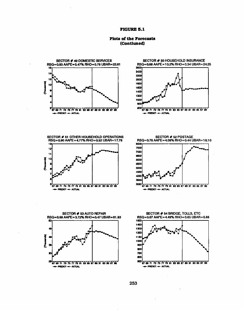
P lots o f the Forecasts (C ontinued)

FIGURE 5.1

SECTOR # 49 DOMESTIC SERVICES SECTOR # 50 HOUSEHOLD INSURANCERSQ»0l83 AAPE“ 5.47% RHO“ Q.78 UBAR=22.61 RSQ=0.68 AAPE=10.2% RHO=0.34 UBAR=24.25

SECTOR # 51 OTHER HOUSEHOLD OPERATIONS SECTOR # 52 POSTAGERSQ=0.90 AAPE=4.77% RHO=0.52 UBAR=17.78 RSQ=0.78 AAPE«4.09% RHO=0.44 UBAR=16.10

SECTOR # 53 AUTO REPAIR RSQ=0.88 AAPE=3.72% RHO=a47 UBAR=61.83

SECTOR # 54 BRIDGE. TOLLS, ETC RSQ=0.67 AAPE=4.49% RHO=0.65 UBAR=0.88

1G0Dt

67 69 71 73 76 77 79 81 83 86 67 89 91 93 96 97 99 t~ PREDICT- • • • ACTUAL

253

P lots o f the Forecasts (C ontiuned)

FIGURE 5.1

SECTOR # 55 AUTO INSURANCE RSQ=0.98 AAPE=2.21 % RHO=0.51 UBAR=15.13 RSQ:

SECTOR # 56 TAXICABS =0.71 AAPE=5.72% RHO=0.68 U BAR=-9.06

SECTOR # 57 LOCAL PUBUC TRANSPORT RSQ=0.51 AAPE=6.07% RHQ=0.63 UBAR=11.72

SECTOR # 58 INTERCITY RAILROAD =0.71 AAPE-7.52% RHO=a72 UBAR=1.26

69 71 73 76 77 79 81 83 85 87 6991 93 96 97 99 ■ - PRBXT « •-- ACTUM.

SECTOR # 59 INTERCITY BUSES RSQ=a 88 AAPE=6.29% RHQ=a50 UBAR=a27

SECTOR# 60 AIRUNES

■ PRBXTT-*-ACTUM.

254

P lots o f the Forecasts (C ontiuned)

FIGURE 5.1

SECTOR # 61 TRAVEL AGENTS AND OTHER RSQ=0.98 AAPE=3.72% RHO=Q.49 UBAR=1.25

SECTOR # 62 CLEANING, LAUNDERING RSQ=0.07 AAPE=6.24% RHO=0.72 UBAR=14.98

SECTOR # 63 BARBERSHOPS AND BEAUTY SHOP RSQ=0.05 AAPE=5.30% RHO=0.64 UBAR=13.95

SECTOR # 64 PHYSICIANS RSQ=0.98 AAPE=Z06% RHO *=0.60 UBAR=73.04

SECTOR # 65 DENTISTS AND OTHER SERVICES RSQ=0.96 AAPE=6.98% RHO=O.S9 UBAR=48.57

SECTOR # 66 PRIVATE HOSPITALS RSQ=0.97 AAPE=3.58% RHO=0.69 UBAR=195.1

255

P lots o f the Forecasts (Contiuned)

FIGURE 5.1

SECTOR # 67 HEALTH INSURANCE RSQ=0.97 AAPE=ai 9% RHO=0.30 UBAR=20.71

SECTOR # 68 BROKERAGE AND INVESTMENT

• PRHUCT ACTUAL

SECTOR # 69 BANK SERVICE CHARGES SECTOR # 70 LIFE INSURANCERSQ=0.99 AAPE=1.95% RHO=0.22 UBAR=91.02 RSQ= a 99 AAPE=1.95% RHO=0.22 UBAR=91.02

SECTOR # 71 LEGAL SERVICES RSQ=0.98 AAPE=2^2% RHO=Q.53 UBAR=34.90 26-24-

22-20-

1fr

1fr

14-

12-

1 77 7B'81 83 B5 B7 89 flfl 83 95 97 99-t» - PRHKTT ACTUAL

SECTOR # 72 FUNERAL EXPENSES AND OTHER RSQ=0.97 AAPE=1.93% RHQ=0.44 UBAR=24.66

256

P lots o f th e Forecasts (C ontinued)

FIGURE 5.1

SECTOR # 73 RADIO AND TV REPAIR RSQ=0.90 AAPE=4.89% RHO=0.64 UBAR=-3.81

SECTOR # 74 MOVIES, LEGITIMATE THEATRE RSQ=0.76 AAPE«=5-84% RHO=a71 UBAR=57.83

SECTOR # 75 OTHER RECREATIONAL SERVICES RSQ=0.99 AAPE=4.78% RHQ=0.68 U BAR-5a 41

SECTOR # 76 EDUCATION

PRBXCT-

SECTOR # 77 RELIGIOUS AND WELFARE RSQ=0.99 AAPE=1.95% RHO=0.59 UBAR=564.4

SECTOR # 78 FOREIGN TRAVEL RSQ=0.23 AAPE=111.5% RHO=0.69 UBAR=59.0

257

m. Outlook

The U.S. economy has continued to expand fo r seven years from 1983 to

1989. D uring th is period, grow th in rea l consum ption averaged 3.8% per year. For

the la s t decade, grow th in consum er expenditures averaged 2.9% from 1979 to 1989.

O ur forecast resu lts , however, show a tendency o f som ewhat weak consum er

spending. The forecasted grow th in consum ption fo r the next decade is m uch slower

th a n the grow th in the 1980’s. The forecasted average grow th rate o f to ta l

consum ption is 1.6% fo r the 1989-1999 period. F igure 5.2 shows the bar chart o f

grow th rates in PCE during the past and the next decades by to ta l consum ption,

durable goods, nondurable goods, and services.

FIGURE 5.2

PERSONAL CONSUMPTION EXPENDITURES ANNUAL GROWTH RATES (%)

6-t

PCE TOTALDURABLE GOODSIZ3NONDURABLE GOODSs sSERVICES

258

The re la tive ly slower grow th In consum er spending over the forecast period

can be accounted fo r by incom e and dem ographic factors. The 1979-1989 period

had strong grow th in Incom e, popula tion, and the num ber o f households. Real

disposable Incom e per capita grew a t an average annual ra te o f 1.6%. The forecast

fo r 1989-1999, however. Is a t m uch slower 0.8% annual grow th. T ota l popula tion

and the num ber o f households, compared w ith the past decade, w ill grow slow ly over

the next ten years. In add ition , the p roportion o f the o lder age groups w ill increase

in the age d is trib u tio n o f the popula tion. Th is dem ographic change w ill p a rticu la rly

low er the demand fo r housing and housing-related consum ption.

The sh ifts in popula tion com positions m ay also account fo r the sh rink ing

consum er budget shares fo r o ther sectors. For Instance, the consum ption item

w hich is m ostly consumed by the baby-boom ers w ill decrease its budget share as the

baby-boom ers clim b in to the next age group. An example Is the alcohol consum ption

on prem ises.

The sluggish grow th in the G asoline. A uto repa ir, and A uto Insurance

sectors are associated w ith the slow grow th o f the car sales over the forecast period.

A uto sales are driven by popula tion grow th, rea l incom e, and other dem ographic

facto rs. S low ing popula tion grow th and the decrease in the num ber o f cars per adu lt

m ay account fo r m ost o f the slow grow th in auto and auto-re lated expenditures.

F igure 5.3 illu s tra te s annual grow th rates o f consum er spending on auto sales, auto

re p a ir and insurance, and gasoline fo r the fo llow ing periods: 1983-1989,1989-1995,

and 1995-2000.

259

FIGURE 5.3

AUTO AND AUTO-RELATED CONSUMER SPENDING ANNUAL GROWTH RATES (%)

260

Besides the slow grow th in consum er spending, the com position o f personal

consum ption expenditures w ill continue to s h ift. F igure 5.4 represents the cha rt o f

shares in PCE by three m ajor categories: durable goods, nondurable goods, and

services, fo r the years 1979, 1989, and 1999. The share o f services w ill increase

faste r than th a t o f nondurable and durable goods. Spending on nondurable goods

has been the weakest among the three groups and w ill continue to decrease its share

in to ta l consum ption. D urable goods w ill rem ain about the same proportion o f to ta l

expenditures.

FIGURE 5.4

THE COMPOSITION OF PCE

261

IV . C onclusions

O ur goal o f estim ating a system o f demand equations and forecasting

personal consum ption expenditures is accom plished. We analyzed the cross-

sectional effects o f incom e and dem ographic variab les, derived a technique fo r

representing the size d is trib u tio n o f incom e, and estim ated the price effects in the

tim e series. These m ethods were effectively Integrated in to the forecasting scheme.

The great advantage o f ou r system is its a b ility to accommodate alm ost a ll

the available economic and dem ographic in fo rm ation . That is , eveiy movement in

the econom ic o r the noneconom ic factors w ill affect the aggregate demand through

o u r specification o f the m odel. However, there is s till the p o ss ib ility fo r our system

to Include some other detailed economic or noneconomic activ ities. For instance,

in te rest rates and stock m arket variab les can be u tilize d to estim ate the sector

Brokerage and investm ent counseling fo r a m ore accurate p red iction .

The sector Foreign trave l is the equation w ith the poorest f it over the

estim ation periods. This re su lt is expected because the expenditure on Foreign trave l

is defined as net spending. It w ould be be tte r if we can handle separately the

am ount U.S. citizens spent In the foreign countries and the am ount foreigners

consum ed in the U.S. ra th e r than dealing, as a t present, w ith the net purchases.

Thus, a fu rth e r research m ay provide a great Im provem ent in th is sector.

In the section on income d is trib u tio n , we should incorporate the la test data

available from S ta tis tics o f Incom e (from 1983 to 1987) fo r constructing the updated

size d is trib u tio n o f incom e. O ur lncom e-expenditure re la tionsh ip m ight be very

sensitive to the size d is trib u tio n o f incom e because o f the fu n ctio n a l form o f the

non linear Engel curve (PLEC). This e ffo rt w ill be undertaken in la te r research.

Furtherm ore, the data source used fo r the cross-sectional analysis, the

262

Consum er E xpenditure Survey, Interview Survey, is available fo r 1989. A

reestim ation o f the cross-section equations w ith new data m ay benefit the system by

a set o f updated "cross-section-prediction" param eters. Th is im provem ent w ill also

be included in the fu rth e r studies.

263

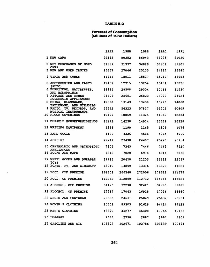
Forecast o f C onsum ption (M illio n s o f 1982 D ollars)

TABLE 5.2

1987

1 NEW CARS 79143

2 NET PURCHASES OF USED 31339 CARS

3 NEW AND USED TRUCKS 25467

4 TIRES AND TUBES 14778

5 ACCESSORIES AND PARTS 12451 (AUTO)

6 FURNITURE, MATTRESSES, 26864 AND BEDSPRINGS

7 KITCHEN AND OTHER 24607 HOUSEHOLD APPLIANCES

8 CHINA, GLASSWARE, 12588 TABLEWARE, AND UTENSILS

9 RADIO, TV, RECORDS, AND 55592 MUSICAL INSTRUMENTS

10 FLOOR COVERINGS 10199

11 DURABLE HOUSEFURNISHINGS 13272

12 WRITING EQUIPMENT 1223

13 HAND TOOLS 4186

14 JEWELRY 22719

15 OPHTHALMIC AND ORTHOPEDIC 7304 APPLIANCES

16 BOOKS AND MAPS 6842

17 WHEEL GOODS AND DURABLE 19926 TOYS

18 BOATS, RV, AND AIRCRAFT 13910

19 FOOD, OFF PREMISE 261402

20 FOOD, ON PREMISE 112262

21 ALCOHOL, OFF PREMISE 31170

22 ALCOHOL, ON PREMISE 17767

23 SHOES AND FOOTWEAR 23636

24 WOMEN'S CLOTHING 85402

25 MEN'S CLOTHING 43370

26 LUGGAGE 2636

27 GASOLINE AND O IL 103302

1988 1989 1990 1991

80382 86943 88925 89030

31337 34829 37809 39103

27046 25135 24817 26685

15011 15537 15719 16083

12715 13254 13481 13836

28508 29304 30466 31530

25691 26823 28022 28924

13143 13438 13796 14060

56323 57837 59702 60809

10869 11325 11869 12334

14238 14904 15669 16328

1199 1165 1109 1076

4326 4586 4764 4969

23490 24407 25220 25954

7343 7446 7465 7520

7020 6974 6846 6858

20458 21203 21811 22537

14899 13316 13329 14221

266348 272056 276618 281478

112899 112712 114866 116827

32298 32421 32780 32882

17043 16918 17026 16660

24531 25049 25632 26231

89303 91629 94414 97121

45277 46408 47765 49133

2790 2887 2997 3109

102671 102786 101139 100471

264

TABLE 5.2

Forecast of Consumption(Millions of 1982 Dollars)

(Continued)

28 FUEL O IL AND COAL

29 TOBACCO

30 SEMIDURABLE HOUSE- FURNISHINGS

31 DRUG PREPARATIONS AND SUNDRIES

32 TOILET ARTICLES AND PREPARATIONS

33 STATIONERY AND WRITING SUPPLIES

34 NONDURABLE TOYS AND SPORT SUPPLIES

35 FLOWERS, SEEDS, AND POTTED PLANTS

36 CLEANING PREPARATIONS

37 LIGHTING SUPPLIES

38 HOUSEHOLD PAPER PRODUCTS

39 MAGAZINES AND NEWSPAPER

40 OTHER NONDURABLES — IDENTITY

41 OWNER OCCUPIED SPACE RENT

42 TENANT OCCUPIED SPACE RENT

43 HOTELS AND MOTELS

44 OTHER HOUSING — EDUCATIONAL HOUSING

45 ELECTRICITY

46 NATURAL GAS

47 WATER AND OTHER SANITARY SERVICES

48 TELEPHONE AND TELEGRAPH

49 DOMESTIC SERVICES

50 HOUSEHOLD INSURANCE

51 OTHER HOUSEHOLD OPERATIONS - REPAIR

52 POSTAGE

53 AUTO REPAIR

54 BRIDGE, TOLLS, ETC.

1987 1988 1989 1990 1991

19393 19869 19679 19905 20046

23000 23018 23129 23235 23356

12546 13132 13401 13761 14019

22208 22667 22570 22120 21972

21557 22133 22577 23154 23701

6001 6230 6243 6176 6245

21939 22393 23259 23800 24514

5802 5791 5801 6024 6158

2443 2342 2419 2406 2415

11004 10572 10498 10038 9770

8679 8556 8728 8641 8675

11260 11395 11225 10920 10852

3105 3144 3209 3275 3343

255531 263165 269394 278716 285822

90145 87343 87522 88139 68660

10515 10755 11043 11331 11633

3924 4057 4124 4176 4254

50514 52538 54379 57146 59438

24477 25110 25751 26489 27146

12643 13155 14128 14505 15025

35162 34099 34513 34396 35198

8776 8283 8116 7653 7297

1459 1470 1532 1515 1551

10948 10831 11227 11229 11513

5607 6100 6786 7015 7159

43380 43004 43556 43150 43080

1256 1239 1231 1194 1164

265

TABLE 5.2

Forecast of Consumption(Millions of 1982 Dollars)

(Continued)

55 AUTO INSURANCE

56 TAXICABS

57 LOCAL PUBLIC TRANSPORT

58 INTERCITY RAILROAD

59 INTERCITY BUSES

60 AIRLINES

61 TRAVEL AGENTS AND OTHER TRANSPORTATION SERVICES

62 CLEANING, LAUNDERING AND SHOE REPAIR

63 BARBERSHOPS AND BEAUTY SHOPS

64 PHYSICIANS

65 DENTISTS AND OTHER PROFESSIONAL SERVICES

66 PRIVATE HOSPITALS AND SANITARIUMS

67 HEALTH INSURANCE

68 BROKERAGE AND INVESTMENT COUNSELING

69 BANK SERVICES CHARGES AND SERVICES WITHOUT PAYMENT

70 L IF E INSURANCE

71 LEGAL SERVICES

72 FUNERAL EXPENSES AND OTHER! PERSONAL BUSINESS

73 RADIO AND TELEVISION REPAIR

74 MOVIES, LEGITIMATE THEATRI AND SPECTATOR SPORTS

75 OTHER RECREATIONAL SERVICES

76 EDUCATION

77 RELIGIOUS AND WELFARE SERVICES

78 FOREIGN TRAVEL

1987 1988 1989 1990 1991

9778 9761 9953 9897 9931

3021 2969 2946 2882 2815

3591 3288 3326 3323 3312

591 579 589 631 679

1061 1033 1026 1016 1017

22575 24382 24533 25007 26051

1749 1831 1911 1993 2075

13103 13214 13211 13319 13351

13096 13395 13485 13695 13867

63149 63714 64339 65300 65970

50094 51582 52987 54736 56312

139083 141986 145659 150351 154100

16898 17100 17334 17461 17669

15631 16083 16378 16673 17026

60853 62171 63367 64466 65757

31727 32486 32947 33294 33683

22413 22623 22947 23177 23604

16382 16221 15651 15435 15157

2554 2449 2418 2305 2235

lf 12319 12562 13114 13595 13724

51870 52745 55266 57538 59741

40987 41819 42525 43254 441880

58044 59282 60422 61558 62942

6707 7258 7414 7639 7870

266

TABLE 5.2

Forecast of Consumption(Millions of 1982 Dollars)

(Continued)

1992

1 NEW CARS 88477

2 NET PURCHASES OF USED 40302 CARS

3 NEW AND USED TRUCKS 28024

4 TIRES AND TUBES 16290

5 ACCESSORIES AND PARTS 14110 (AUTO)

6 FURNITURE, MATTRESSES, 32526 AND BEDSPRINGS

7 KITCHEN AND OTHER 29673 HOUSEHOLD APPLIANCES

8 CHINA, GLASSWARE, 14230 TABLEWARE, AND UTENSILS

9 RADIO, TV, RECORDS, AND 61301 MUSICAL INSTRUMENTS

10 FLOOR COVERINGS 12691

11 DURABLE HOUSEFURNISHINGS 16863

12 WRITING EQUIPMENT 1037

13 HAND TOOLS 5133

14 JEWELRY 26761

15 OPHTHALMIC AND ORTHOPEDIC 7654 APPLIANCES

16 BOOKS AND MAPS 6808

17 WHEEL GOODS AND DURABLE 23088 TOYS

18 BOATS, RV, AND AIRCRAFT 14994

19 FOOD, OFF PREMISE 284378

20 FOOD, ON PREMISE 119163

21 ALCOHOL, OFF PREMISE 33004

22 ALCOHOL, ON PREMISE 16277

23 SHOES AND FOOTWEAR 26709

24 WOMEN'S CLOTHING 99435

25 MEN'S CLOTHING 50246

26 LUGGAGE 3220

27 GASOLINE AND O IL 99290

1994 1996 1998 2000

85611 83284 81911 80914

40966 43167 46466 49059

29965 32086 33335 34442

16579 17143 17405 17597

14543 15039 15443 15774

34137 35976 38235 41178

31765 33932 36981 40316

14667 15036 15774 16616

63316 65421 69025 73376

13029 13513 13836 14348

18098 19436 20964 22919

907 788 649 524

5422 5651 5872 6187

28143 29679 31320 33331

7612 7611 7542 7530

6470 6268 5934 5676

24018 24807 25655 26602

16187 17175 18223 19542

290691 298515 304798 309339

122387 125807 129698 133307

32962 32672 32456 32152

15500 14587 13502 12638

27670 28732 29924 31279

104580 109806 115599 122382

52607 54912 57439 60419

3439 3670 3929 4212

95990 92981 89541 85709

267

TABLE 8.2

Forecast of Consumption(Millions of 1982 Dollars)

(Continued)

28 FUEL O IL AND COAL

29 TOBACCO

30 SEMIDURABLE HOUSE- FURNISHINGS

31 DRUG PREPARATIONS AND SUNDRIES

32 TOILET ARTICLES AND PREPARATIONS

33 STATIONERY AND WRITING SUPPLXES

34 NONDURABLE TOYS AND SPORT SUPPLIES

35 FLOWERS, SEEDS, AND POTTED PLANTS

36 CLEANING PREPARATIONS

37 LIGHTING SUPPLIES

38 HOUSEHOLD PAPER PRODUCTS

39 MAGAZINES AND NEWSPAPER

40 OTHER NONDURABLES — IDENTITY

41 OWNER OCCUPIED SPACE RENT

42 TENANT OCCUPIED SPACE RENT

43 HOTELS AND MOTELS

44 OTHER HOUSING — EDUCATIONAL HOUSING

45 ELECTRICITY

46 NATURAL GAS

47 WATER AND OTHER SANITARY SERVICES

48 TELEPHONE AND TELEGRAPH

49 DOMESTIC SERVICES

50 HOUSEHOLD INSURANCE

51 OTHER HOUSEHOLD OPERATIONS - REPAIR

52 POSTAGE

53 AUTO REPAIR

54 BRIDGE, TOLLS, ETC.

1992 1994 1996 1998 2000

20080 20402 20730 21120 21383

23405 23497 23603 23717 23727

14204 14743 15247 16032 16946

21848 21003 20181 19091 18116

24104 24865 25366 26100 27054

6259 6088 6075 5932 5910

25096 25927 26685 27429 28231

6294 6475 6582 6631 6811

2410 2319 2189 2084 2012

9381 8332 7245 6255 5417

8681 8516 8283 8072 7798

10727 10043 9518 8770 8192

3401 3500 3585 3681 3780

292571 316488 339006 368266 399471

89151 92640 95408 98790 101094

11927 12395 12744 13082 13463

4352 4497 4619 4686 4731

61445 66768 71346 76674 81869

27667 29118 30363 31871 33279

15519 16407 16932 17417 17680

35692 36685 37564 37951 38054

6886 5848 4926 4218 3660

1541 1522 1547 1556 1557

11685 11612 11505 11373 11296

7472 7570 7394 7346 7270

42707 41686 40717 39868 38909

1124 1031 936 840 737

268

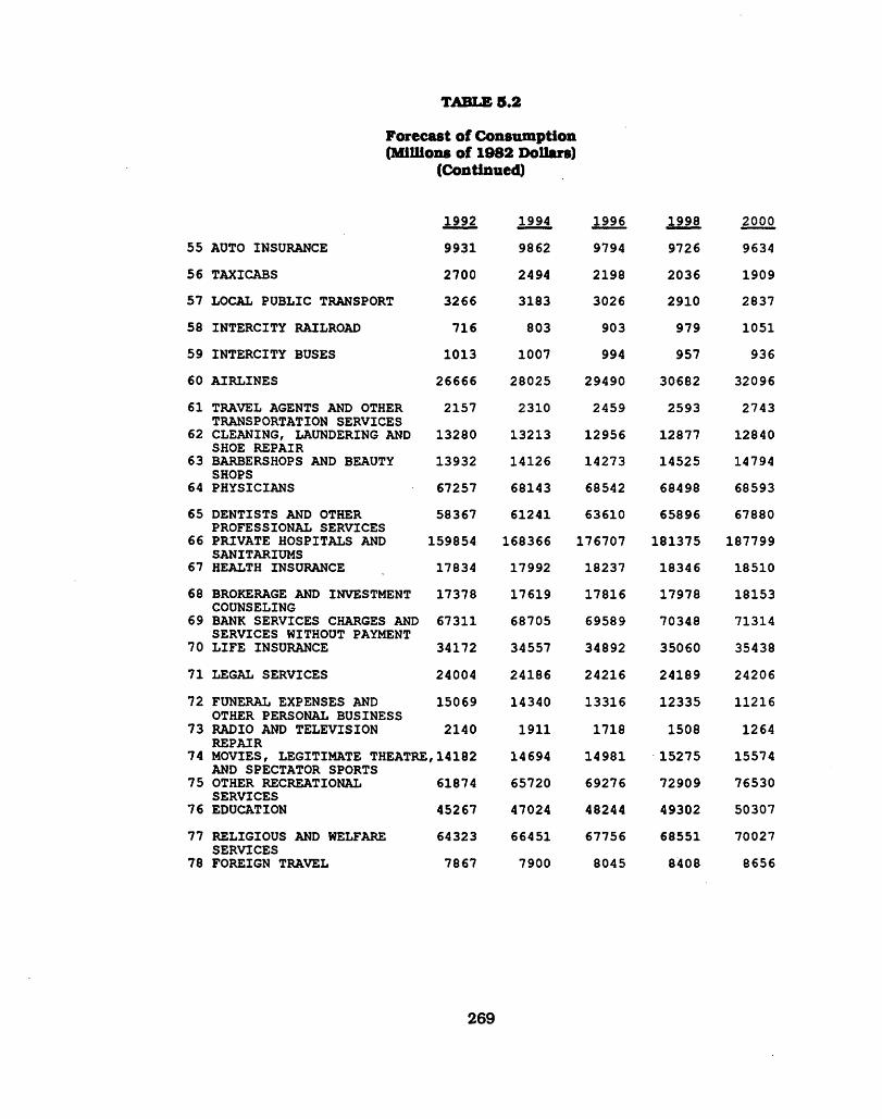
TABLE 5.2

Forecast of Consumption(Millions of 1982 Dollars)

(Continued)

55 AUTO INSURANCE

1992

9931

56 TAXICABS 2700

57 LOCAL PUBLIC TRANSPORT 3266

58 INTERCITY RAILROAD 716

59 INTERCITY BUSES 1013

60 AIRLINES 26666

61 TRAVEL AGENTS AND OTHER 2157

62TRANSPORTATION SERVICES CLEANING, LAUNDERING AND 13280

63SHOE REPAIR BARBERSHOPS AND BEAUTY 13932

64SHOPSPHYSICIANS 67257

65 DENTISTS AND OTHER 58367

66PROFESSIONAL SERVICES PRIVATE HOSPITALS AND 159854

67SANITARIUMS HEALTH INSURANCE 17834

68 BROKERAGE AND INVESTMENT 17378

69COUNSELINGBANK SERVICES CHARGES AND 67311

70SERVICES WITHOUT PAYMENT L IF E INSURANCE 34172

71 LEGAL SERVICES 24004

72 FUNERAL EXPENSES AND 15069

73OTHER PERSONAL BUSINESS RADIO AND TELEVISION 2140

74REPAIRMOVIES, LEGITIMATE THEATRE ,14182

75AND SPECTATOR SPORTS OTHER RECREATIONAL 61874

76SERVICESEDUCATION 45267

77 RELIGIOUS AND WELFARE 64323

78SERVICES FOREIGN TRAVEL 7867

1994 1996 1998 2000

9862 9794 9726 9634

2494 2198 2036 1909

3183 3026 2910 2837

803 903 979 1051

1007 994 957 936

28025 29490 30682 32096

2310 2459 2593 2743

13213 12956 12877 12840

14126 14273 14525 14794

68143 68542 68498 68593

61241 63610 65896 67880

168366 176707 181375 187799

17992 18237 18346 18510

17619 17816 17978 18153

68705 69589 70348 71314

34557 34892 35060 35438

24186 24216 24189 24206

14340 13316 12335 11216

1911 1718 1508 1264

14694 14981 15275 15574

65720 69276 72909 76530

47024 48244 49302 50307

66451 67756 68551 70027

7900 8045 8408 8656

269

TABLE 5.3

G row th Rates (Percent)

1 NEW CARS

87-88

1 .5 6 5

8 8 -89

8 .1 6 2

8 9 -90

2 .2 8 0

90-91

0 .1 1 7

91-92

-0 .6 2 0

2 NET PURCHASES OF USED -0 .0 0 8 1 1 .1 4 3 8 .5 5 7 3 .4 2 4 3 .0 6 5

3CARSNEW AND USED TRUCKS 6 .2 0 0 -7 .0 6 6 -1 .2 6 6 7 .5 2 5 5 .0 2 1

4 TIRES AND TUBES 1 .5 7 6 3 .5 0 2 1 .1 7 5 2 .3 1 5 1 .2 8 6

5 ACCESSORIES AND PARTS 2 .1 2 5 4 .2 3 3 1 .1 7 2 2 .6 3 6 1 .9 7 5

6(AUTO)FURNITURE, MATTRESSES, 6 .1 2 1 2 .7 9 2 3 .9 6 6 3 .4 9 2 3 .1 5 9

7AND BEDSPRINGS KITCHEN AND OTHER 4 .4 0 3 4 .4 0 7 4 .4 7 1 3 .2 1 9 2 .5 8 8

8HOUSEHOLD APPLIANCES CHINA, GLASSWARE, 4 .4 0 9 2 .2 4 6 2 .6 6 9 1 .9 0 6 1 .2 1 6

9TABLEWARE, AND UTENSILS RADIO, TV, RECORDS, AND 1 .3 1 5 2 .6 8 7 3 .2 2 5 1 .8 5 4 0 .80 8

10MUSICAL INSTRUMENTS FLOOR COVERINGS 6 .5 6 6 4 .2 0 3 4 .7 9 6 3 .9 1 7 2 .8 9 6

11 DURABLE HOUSEFURNISHINGS 7 .2 7 8 4 .6 7 9 5 .1 3 5 4 .2 0 5 3 .27 4

12 WRITING EQUIPMENT -2 .0 2 5 -2 .8 4 8 -4 .7 8 7 -2 .9 2 4 -3 .7 0 3

13 HAND TOOLS 3 .3 4 9 6 .0 0 1 3 .8 8 5 4 .3 0 6 3 .29 2

14 JEWELRY 3 .3 9 0 3 .9 0 5 3 .3 3 2 2 .9 1 0 3 .10 8

15 OPHTHALMIC AND ORTHOPEDIC 0 .5 3 7 1 .3 9 9 0 .2 5 8 0 .7 3 7 1 .7 7 5

16APPLIANCES BOOKS AND MAPS 2 .5 9 8 -0 .6 5 2 -1 .8 3 9 0 .1 8 7 -0 .7 3 7

17 WHEEL GOODS AND DURABLE 2 .6 6 8 3 .6 4 3 2 .8 6 8 3 .3 2 7 2 .4 4 5

18TOYSBOATS, RV, AND AIRCRAFT 7 .1 1 3 -1 0 .6 2 4 0 .0 9 1 6 .6 9 9 5 .43 4

19 FOOD, OFF PREMISE 1 .8 9 2 2 .1 4 3 1 .6 7 7 1 .7 5 7 1 .03 0

20 FOOD, ON PREMISE 0 .5 6 8 -0 .1 6 6 1 .9 1 1 1 .7 0 8 1 .9 9 9

21 ALCOHOL, OFF PREMISE 3 .61 7 0 .3 8 2 1 .1 0 6 0 .3 1 2 0 .37 2

22 ALCOHOL, ON PREMISE -4 .0 7 4 -0 .7 3 2 0 .6 3 6 -2 .1 4 4 -2 .3 0 1

23 SHOES AND FOOTWEAR 3 .7 8 4 2 .1 1 5 2 .3 2 6 2 .3 3 8 1 .8 2 2

24 WOMEN'S CLOTHING 4 .5 6 8 2 .6 0 4 3 .0 3 9 2 .8 6 7 2 .2 8 3

25 MEN'S CLOTHING 4 .3 9 6 2 .4 9 8 2 .9 2 4 2 .8 6 4 2 .2 6 6

26 LUGGAGE 5 .8 5 7 3 .4 7 0 3 .8 1 2 3 .7 3 1 3 .59 7

27 GASOLINE AND O IL -0 .6 1 1 0 .1 1 2 -1 .6 0 3 -0 .6 6 0 -1 .1 7 6

270

TABLE 5.3

G row th Rates (Percent)

(C ontinued)

87-88 8 8 -89 8 9 -90 90 -91 91 -9 2

28 FUEL O IL AND COAL 2 .4 5 7 -0 .9 5 9 1 .1 5 1 0 .7 0 5 0 . 170

29 TOBACCO 0 .0 7 6 0 .4 8 4 0 .4 5 8 0 .5 2 2 0 . 207

30 SEMIDURABLE HOUSE- FURNISHIN6S

4 .6 7 4 2 .0 4 6 2 .6 8 6 1 .8 7 6 1 . 324

31 DRUG PREPARATIONS AND SUNDRIES

2 .0 6 9 -0 .4 2 8 -1 .9 9 3 - 0 .6 7 1 - 0 . 562

32 TOILET ARTICLES AND PREPARATIONS

2 .6 7 4 2 .0 0 4 2 .5 5 6 2 .3 6 2 1 . 703

33 STATIONERY AND WRITING SUPPLIES

3 .8 2 1 0 .1 9 8 -1 .0 7 1 1 .1 2 1 0 . 232

34 NONDURABLE TOYS AND SPORT SUPPLIES

2 .0 6 8 3 .8 6 9 2 .3 2 4 2 .9 9 9 2 . 377

35 FLOWERS, SEEDS, AND POTTED PLANTS

-0 .1 9 4 0 .1 7 6 3 .8 5 3 2 .2 2 4 2 . 197

36 CLEANING PREPARATIONS -4 .1 3 2 3 .2 5 1 -0 .5 3 4 0 .3 7 7 - 0 . 188

37 LIGHTING SUPPLIES -3 .9 2 1 -0 .7 0 5 -4 .3 8 4 -2 .6 6 8 - 3 . 984

38 HOUSEHOLD PAPER PRODUCTS -1 .4 1 5 2 .0 1 9 -1 .0 0 4 0 .3 9 5 0 . 069

39 MAGAZINES AND NEWSPAPER 1 .1 9 9 -1 .4 9 0 -2 .7 1 8 -0 .6 2 4 - 1 . 146

40 OTHER NONDURABLES - - IDENTITY

1 .2 3 5 2 .0 7 0 2 .0 6 8 2 .0 5 3 1. 751

41 OWNER OCCUPIED SPACE RENT

2 .9 8 8 2 .3 6 7 3 .4 6 0 2 .5 5 0 2 . 361

42 TENANT OCCUPIED SPACE RENT

-3 .1 0 9 0 .2 0 4 0 .7 0 6 0 .5 9 1 0. 554

43 HOTELS AND MOTELS 2 .2 7 9 2 .6 7 8 2 .6 1 0 2 .6 6 3 2 . 530

44 OTHER HOUSING — EDUCATIONAL HOUSING

3 .3 7 9 1 .6 4 8 1 .2 6 8 1 .8 6 5 2 . 300

45 ELECTRICITY 4 .0 0 6 3 .50 4 5 .0 8 9 4 .0 1 0 3. 376

46 NATURAL GAS 2 .5 8 6 2 .5 5 2 2 .8 6 8 2 .4 7 7 1 . 921

47 WATER AND OTHER SANITARY SERVICES

4 .0 4 7 7 .3 9 9 2 .6 6 8 3 .5 8 4 3. 289

48 TELEPHONE AND TELEGRAPH -3 .0 2 4 1 .2 1 6 -0 .3 4 0 2 .3 3 2 1. 403

49 DOMESTIC SERVICES -5 .6 1 9 -2 .0 0 8 -5 .7 1 1 -4 .6 4 8 - 5 . 633

50 HOUSEHOLD INSURANCE 0 .7 1 3 4 .2 1 4 -1 .0 6 6 2 .3 4 8 - 0 . 639

51 OTHER HOUSEHOLD OPERATIONS - REPAIR

-1 .0 6 7 3 .6 6 0 0 .0 1 6 2 .5 2 7 1. 497

52 POSTAGE 8 .7 8 2 1 1 .2 58 3 .3 6 8 2 .0 4 9 4 . 382

53 AUTO REPAIR -0 .8 6 7 1 .2 8 5 -0 .9 3 2 -0 .1 6 3 - 0 . 864

54 BRIDGE, TOLLS, ETC. -1 .3 1 9 -0 .6 1 3 -3 .0 3 9 -2 .4 9 4 - 3 . 421

271

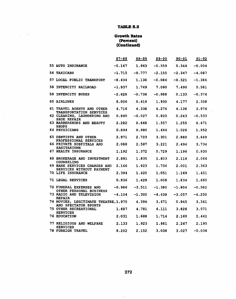
TABLE 5.3

G row th Rates (Percent)

(C ontinued)

55 AUTO INSURANCE

87-88

-0 .1 6 7

88 -89

1 .9 6 3

8 9-90

-0 .5 5 9

90-91

0 .3 4 4

9 1-92

-0 .0 0 4

56 TAXICABS -1 .7 1 5 -0 .7 7 7 -2 .1 5 5 -2 .3 4 7 -4 .0 8 7

57 LOCAL PUBLIC TRANSPORT -8 .4 3 4 1 .1 3 6 -0 .0 8 4 -0 .3 2 1 -1 .3 8 6

58 INTERCITY RAILROAD -1 .9 3 7 1 .7 4 9 7 .0 9 0 7 .4 9 0 5 .58 1

59 INTERCITY BUSES -2 .6 2 8 -0 .7 3 6 -0 .9 8 8 0 .1 3 3 -0 .3 7 4

60 AIRLINES 8 .0 0 6 0 .6 1 9 1 .9 3 0 4 .1 7 7 2 .3 5 8

61 TRAVEL AGENTS AND OTHER 4 .7 1 6 4 .3 3 8 4 .2 7 6 4 .1 3 8 3 .9 7 4

62TRANSPORTATION SERVICES CLEANING, LAUNDERING AND 0 .8 4 5 -0 .0 2 7 0 .8 2 0 0 .2 4 3 -0 .5 3 3

63SHOE REPAIR BARBERSHOPS AND BEAUTY 2 .2 8 2 0 .6 6 8 1 .5 5 7 1 .2 5 5 0 .4 7 1

64SHOPSPHYSICIANS 0 .8 9 4 0 .9 8 0 1 .4 9 4 1 .0 2 6 1 .9 5 2

65 DENTISTS AND OTHER 2 .9 7 1 2 .7 2 3 3 .3 0 1 2 .8 8 0 3 .6 4 9

66PROFESSIONAL SERVICES PRIVATE HOSPITALS AND 2 .0 8 8 2 .5 8 7 3 .2 2 1 2 .4 9 4 3 .73 4

67SANITARIUMS HEALTH INSURANCE 1 .1 9 2 1 .3 7 2 0 .7 2 9 1 .1 9 6 0 .9 3 0

68 BROKERAGE AND INVESTMENT 2 .8 9 1 1 .8 3 5 1 .8 0 3 2 .1 1 6 2 .0 6 6

69COUNSELINGBANK SERVICES CHARGES AND 2 .1 6 6 1 .9 2 3 1 .7 3 6 2 .0 0 1 2 .3 6 3

70SERVICES WITHOUT PAYMENT L IF E INSURANCE 2 .3 9 4 1 .4 2 0 1 .0 5 1 1 .1 6 9 1 .4 5 1

71 LEGAL SERVICES 0 .9 3 6 1 .4 2 9 1 .0 0 8 1 .8 3 4 1 .6 9 5

72 FUNERAL EXPENSES AND -0 .9 8 6 -3 .5 1 1 -1 .3 8 0 -1 .8 0 4 -0 .5 8 2

73OTHER PERSONAL BUSINESS RADIO AND TELEVISION -4 .1 0 4 -1 .3 0 0 -4 .6 3 8 -3 .0 5 7 -4 .2 5 0

74REPAIRMOVIES, LEGITIMATE THEATRE1,1.970 4 .3 9 4 3 .6 7 1 0 .9 4 5 3 .3 4 1

75AND SPECTATOR SPORTS OTHER RECREATIONAL 1 .6 8 7 4 .7 8 1 4 .1 1 1 3 .8 2 8 3 .5 7 1

76SERVICESEDUCATION 2 .0 3 1 1 .6 8 8 1 .7 1 4 2 .1 6 0 2 .4 4 2

77 RELIGIOUS AND WELFARE 2 .1 3 3 1 .9 2 3 1 .8 8 1 2 .2 4 7 2 .1 9 5

78SERVICES FOREIGN TRAVEL 8 .2 0 2 2 .1 5 2 3 .0 3 8 3 .0 2 7 -0 .0 3 6

272

TABLE 8.3

G row th Rates (Percent)

(C ontinued)

92-94 9 4-96 96-98 98 -00 88 -0 0

1 NEW CARS -1 .6 3 3 -1 .3 6 9 -0 .8 2 8 -0 .6 0 5 0 . 089

2 NET PURCHASES OF USED CARS

0 .8 2 6 2 .6 6 0 3 .7 5 2 2 .7 5 3 3. 847

3 NEW AND USED TRUCKS 3 .4 0 8 3 .4 9 6 1 .9 2 7 1 .6 5 2 2 . 098

4 TIRES AND TUBES 0 .8 8 4 1 .6 9 0 0 .7 6 2 0 .5 5 4 1. 338

5 ACCESSORIES AND PARTS (AUTO)

1 .5 2 3 1 .6 9 3 1 .3 3 4 1 .0 6 8 1. 816

6 FURNITURE, MATTRESSES, AND BEDSPRINGS

2 .4 4 8 2 .6 5 9 3 .0 9 2 3 .7 7 8 3 . 114

7 KITCHEN AND OTHER HOUSEHOLD APPLIANCES

3 .46 8 3 .3 5 7 4 .3 9 7 4 .4 1 5 3. 830

8 CHINA, GLASSWARE, TABLEWARE, AND UTENSILS

1 .5 6 9 1 .2 5 2 2 .4 2 7 2 .6 3 5 1 . 976

9 RADIO, TV, RECORDS, AND MUSICAL INSTRUMENTS

1 .6 3 2 1 .6 4 9 2 .7 1 8 3 .1 0 4 2 . 232

10 FLOOR COVERINGS 3 .1 9 2 3^044 3 .0 8 3 3 .8 1 0 3 . 506

11 DURABLE HOUSEFURNISHINGS 3 .5 9 9 3 .6 3 2 3 .8 5 8 4 .5 6 0 4. 409

12 WRITING EQUIPMENT -6 .4 3 2 -6 .8 1 5 -9 .2 4 7 -1 0 .1 2 7 - 6 . 625

13 HAND TOOLS 2 .7 7 7 2 .0 9 6 1 .9 3 4 2 .6 4 9 3. 033

14 JEWELRY 2 .5 5 0 2 .6 9 3 2 .7 2 8 3 .1 6 2 2 . 960

15 OPHTHALMIC AND ORTHOPEDIC APPLIANCES

0 .2 6 2 -0 .0 0 4 -0 .7 8 6 -0 .0 7 6 0. 213

16 BOOKS AND MAPS -2 .5 0 7 -1 .5 7 6 -2 .7 0 1 -2 .1 9 5 - 1 . 750

17 WHEEL GOODS AND DURABLE TOYS

1 .9 9 5 1 .6 2 9 1 .6 9 5 1 .8 3 0 2 . 215

18 BOATS, RV, AND AIRCRAFT 3 .9 0 7 3 .0 0 8 3 .0 0 8 3 .5 5 5 2 . 379

19 FOOD, OFF PREMISE 1 .10 4 1 .3 4 0 1 .0 4 7 0 .7 4 6 1. 257

20 FOOD, ON PREMISE 1 .34 4 1 .3 8 9 1 .5 3 5 1 .3 8 2 1. 396

21 ALCOHOL, OFF PREMISE -0 .0 6 5 -0 .4 4 0 -0 .3 3 2 -0 .4 6 9 - 0 . 036

22 ALCOHOL, ON PREMISE -2 .4 1 5 -2 .9 8 2 -3 .7 9 0 -3 .2 5 2 - 2 . 452

23 SHOES AND FOOTWEAR 1 .78 4 1 .9 0 1 2 .0 5 3 2 .2 4 0 2 . 046

24 WOMEN'S CLOTHING 2 .5 5 5 2 .4 6 8 2 .6 0 4 2 .8 9 3 2 . 661

25 MEN'S CLOTHING 2 .3 2 3 2 .1 6 8 2 .2 7 5 2 .5 6 2 2 . 434

26 LUGGAGE 3 .3 4 0 3 .2 9 9 3 .4 7 3 3 .5 3 5 3 . 492

27 GASOLINE AND O IL -1 .6 7 6 -1 .5 8 0 -1 .8 6 8 -2 .1 6 3 - 1 . 491

273

TABLE 5.3

G row th Rates (Percent)

(C ontinued)

28 FUEL O IL AND COAL

92-94

0 .8 0 0

94 -96

0 .8 0 7

96 -98

0 .9 3 7

9 8 -00

0 .6 2 6

88-00

0 .6 1 7

29 TOBACCO 0 .1 9 7 0 .2 2 6 0 .2 4 1 0 .0 2 1 0 .2 5 3

30 SEMIDURABLE HOUSE- 1 .8 8 0 1 .6 9 6 2 .5 4 3 2 .8 1 3 2 .1 4 9

31FURNISHINGSDRUG PREPARATIONS AND -1 .9 5 2 -1 .9 7 4 -2 .7 3 9 -2 .5 8 7 -1 .8 4 6

32SUNDRIESTOILET ARTICLES AND 1 .5 6 5 1 .0 0 6 1 .4 3 7 1 .8 1 2 1 .68 8

33PREPARATIONS STATIONERY AND WRITING -1 .3 7 9 -0 .1 0 1 -1 .1 8 4 -0 .1 8 2 -0 .4 3 4

34SUPPLIESNONDURABLE TOYS AND 1 .6 4 1 1 .4 5 2 1 .3 8 5 1 .4 5 1 1 .9 5 2

35SPORT SUPPLIES FLOWERS, SEEDS, AND 1 .4 3 3 0 .8 2 0 0 .3 7 4 1 .3 4 8 1 .3 6 7

36POTTED PLANTS CLEANING PREPARATIONS -1 .9 0 9 -2 .8 2 9 -2 .4 2 7 -1 .7 3 2 -1 .2 4 1

37 LIGHTING SUPPLIES -5 .7 5 1 -6 .7 4 3 -7 .0 8 0 -6 .9 4 1 -5 .3 9 7

38 HOUSEHOLD PAPER PRODUCTS -0 .9 5 3 -1 .3 8 1 -1 .2 8 2 -1 .7 0 8 -0 .7 6 4

39 MAGAZINES AND NEWSPAPER -3 .2 3 8 -2 .6 4 2 -4 .0 0 7 -3 .3 4 2 -2 .7 0 3

40 OTHER NONDURABLES — 1 .4 3 9 1 .2 0 9 1 .3 4 0 1 .3 3 1 1 .54 8

41IDENTITYOWNER OCCUPIED SPACE 4 .0 0 8 3 .49 7 4 .22 7 4 .1 5 2 3 .54 2

42RENTTENANT OCCUPIED SPACE 1 .9 8 3 1 .4 8 3 1 .7 5 7 1 .1 6 0 1 .22 8

43RENTHOTELS AND MOTELS 1 .9 4 2 1 .3 9 7 1 .3 2 1 1 .4 4 5 1 .8 9 1

44 OTHER HOUSING — 1 .6 5 5 1 .3 5 5 0 .7 1 9 0 .4 7 7 1 .2 9 1

45EDUCATIONAL HOUSING ELECTRICITY 4 .2 4 2 3 .3 7 3 3 .6 6 7 3 .3 3 4 3 .76 7

46 NATURAL GAS 2 .5 8 9 2 .1 1 7 2 .4 5 5 2 .1 8 5 2 .3 7 6

47 WATER AND OTHER 2 .8 2 3 1 .5 8 8 1 .4 2 3 0 .7 5 3 2 .5 0 9

48SANITARY SERVICES TELEPHONE AND TELEGRAPH 1 .3 8 6 1 .1 9 2 0 .5 1 5 0 .1 3 6 0 .9 2 2

49 DOMESTIC SERVICES -7 .8 4 3 -8 .1 7 6 -7 .4 5 8 -6 .8 4 6 -6 .5 5 4

50 HOUSEHOLD INSURANCE -0 .6 2 7 0 .8 4 8 0 .2 6 8 0 .0 4 4 0 .4 9 3

51 OTHER HOUSEHOLD -0 .3 1 2 -0 .4 6 3 -0 .5 7 8 -0 .3 3 8 0 .3 6 0

52OPERATIONS - REPAIR POSTAGE 0 .6 6 1 -1 .1 7 1 -0 .3 2 3 -0 .5 1 5 1 .5 3 0

53 AUTO REPAIR -1 .2 0 3 -1 .1 6 9 -1 .0 4 7 -1 .2 1 0 -0 .8 2 7

54 BRIDGE, TOLLS, ETC. -4 .2 4 6 -4 .7 2 1 -5 .2 7 5 -6 .3 0 0 -4 .2 2 1

274

TABLE 5.3

G row th Rates (Percent)

(C ontinued)

55 AUTO INSURANCE

92-94

-0 .3 4 7

9 4 -96

-0 .3 4 5

96-98

-0 .3 4 8

98-00

-0 .4 7 6 o loo

loo -0 0

107

56 TAXICABS -3 .8 8 2 -5 .9 5 0 -3 .7 3 3 -3 .1 8 1 - 3 . 571

57 LOCAL PUBLIC TRANSPORT -1 .2 8 3 -2 .4 3 7 -1 .9 4 4 -1 .2 5 8 - 1 . 208

58 INTERCITY RAILROAD 5 .9 0 2 6 .0 2 7 4 .1 0 7 3 .6 0 2 5. 099

59 INTERCITY BUSES -0 .3 0 0 -0 .6 3 9 -1 .8 7 1 -1 .1 1 0 - 0 . 817

60 AIRLINES 2 .5 1 8 2 .5 8 0 2 .0 0 2 2 .2 7 9 2 . 320

61 TRAVEL AGENTS AND OTHER 3 .4 7 5 3 .1 6 6 2 .7 0 5 2 .8 2 8 3. 426

62TRANSPORTATION SERVICES CLEANING, LAUNDERING AND -0 .2 5 3 -0 .9 7 9 -0 .3 0 5 -0 .1 4 5 - 0 . 238

63SHOE REPAIR BARBERSHOPS AND BEAUTY 0 .6 9 6 0 .5 2 2 0 .8 7 7 0 .9 2 3 0. 832

64SHOPSPHYSICIANS 0 .6 5 7 0 .2 9 5 -0 .0 3 2 0 .0 7 0 0 . 619

65 DENTISTS AND OTHER 2 .4 3 4 1 .9 1 7 1 .7 8 1 1 .4 9 5 2 . 317

66PROFESSIONAL SERVICES PRIVATE HOSPITALS AND 2 .6 2 9 2 .4 5 2 1 .3 1 4 1 .7 5 8 2 . 361

67SANITARIUMS HEALTH INSURANCE 0 .4 4 3 0 .6 8 2 0 .2 9 9 0 .4 4 6 0 . 664

68 BROKERAGE AND INVESTMENT 0 .6 9 2 0 .8 9 3 0 .4 5 2 0 .4 8 7 1 . 017

69COUNSELINGBANK SERVICES CHARGES AND 1 .0 3 1 0 .6 4 2 0 .5 4 5 0 .6 8 6 1 . 152

70SERVICES WITHOUT PAYMENT L IF E INSURANCE 0 .5 6 1 0 .4 8 5 0 .1 1 6 0 .5 3 7 0 . 728

71 LEGAL SERVICES 0 .3 8 0 0 .0 6 9 -0 .0 5 7 0 .0 3 6 0. 568

72 FUNERAL EXPENSES AND -2 .4 4 7 -3 .6 3 6 -3 .7 5 4 -4 .6 3 4 - 3 . 018

73OTHER PERSONAL BUSINESS RADIO AND TELEVISION -5 .4 9 9 -5 .1 8 1 -6 .2 8 6 -8 .4 4 4 - 5 . 339

74REPAIRMOVIES, LEGITIMATE THEATRE:,1 .7 5 1 0 .9 7 4 0 .9 7 7 0 .9 7 2 1 . 815

75AND SPECTATOR SPORTS OTHER RECREATIONAL 3 .0 6 1 2 .6 7 0 2 .5 8 9 2 .4 5 4 3 . 153

76SERVICESEDUCATION 1 .92 4 1 .2 8 9 1 .0 9 2 1 .0 1 4 1. 553

77 RELIGIOUS AND WELFARE 1 .6 4 2 0 .9 7 9 0 .5 8 5 1 .0 7 3 1 . 400

78SERVICES FOREIGN TRAVEL 0 .2 0 9 0 .9 1 3 2 .2 5 6 1 .5 1 0 1 . 496

275

APPENDIX A

REVIEW OF EMPIRICAL CONSUMPTION FUNCTIONS

The functiona l form s fo r the em pirica l demand system s m ust be appropriate

fo r both theore tica l specification and em pirica l estim ation techniques. We sh a ll not

a ttem pt to provide a detailed review o f the lite ra tu re on consum er dem and, because

m any reviews already exist. Among these are "M odels o f Consum er Behavior: A

Survey" by Brow n and D eaton1 and T he Systems o f Consum er Demand Functions

Approach: A Review” by B arten.2

The m ore recent com prehensive w ork Includes Econom ics and Consum er

Behavior by Deaton and M uellbauer.3 In "A System o f C onsum ption Functions and

Its E stim ation fo r Belgium ," Ahnon4 investigated the shortcom ings o f the existing

dem and system s and suggested an im proved functiona l form . The m ost recent

survey, "Theory and E m pirica l Evidence - A Survey," by B lunde ll5 emphasizes on

the areas o f disaggregate consum er behavior and o f dynam ic and life -cycle consum er

behavior.

The exhaustive French a rtic le , "The Interdependent Systems o f Consum ption

1Brown, J . A. C. and A. S. Deaton (1972), "Models o f Consumer Behavior: A Survey," Economic Journal. Vol. 82, pp. 1145-1236.

2Barten, A. P. (1977), The Systems o f Consumer Demand Functions Approach: A Review," Econometrica. Vol. 45, pp. 23-51.

3Deaton, A. S. and J. Muellbauer (1980b), Economics and Consumer Behavior. Cambridge: Cambridge University Press.

4Almon, C. (1979), nA System o f Consumption Functions and its EstimaUon for Belgium ," Southern Economic Journal. Vol. 46, pp. 85-106.

5B lundell, C. (1988), "Consumer Behavior: Theoiy and Em pirical Evidence - A Survey,” Economic Journal. Vol. 98, pp. 16-65.

276

F unctions," by D anie l Gauyacq6 reviews and sum m arizes alm ost a ll the existing

functions o f consum er dem and, in c lud ing the "A lm ost Ideal Demand System"

developed by Deaton and M uellbauer.7 Gauyacq estim ated each system o f demand

functions using the French data. A general conclusion o f the study is th a t only the

A lm on m odel is , from a p ractica l po in t o f view , convenient fo r determ ination o f

disaggregated demand functions.

Since the appearance o f Ahnon's a rtic le , there is great a tten tion paid to the

"A lm ost Ideal Demand System" m odel. We sha ll, based on A lm on’s c rite ria , extend

th e investiga tion o f the functiona l form s to th is demand system and show th a t it

lacks im portan t features o f a tru ly ideal demand system.

A lm ost Ideal Demand System:

To express th is "A lm ost Ideal" form , le t wt = budget share o f good i; y = to ta l

expenditure; and pt = price o f good i. The system can then be w ritte n as follow s:

+ '£ y iJlogpj + P (log(-p) (A.1)

where P is price index defined by

logp = do + £ “ fclogPfc + iEEYlcllogPfciogp, (A.2)k z k I

The fo llow ing constra in ts on the param eters

E P fc = ° - E Y |j, = 0. and = Y j, (a.3)

ensure th a t the m odel satisfies adding-up, hom ogeneity, and sym m etry.

6Gauyacq, D. (1985), "Les Systemes Interdependants de Fonctions de Consommation Prevision et Analyse Economlciue. Vol. 6, No.2.

7Deaton, A. S. and J. Muellbauer (1980a), "An Almost Ideal Demand System." American Economic Review. Vol. 70, pp. 312-326.

277

The firs t th in g to notice is th a t if any > 0 , then some < 0. For th is i.

increasing incom e w ith constant prices eventually produces a negative budget share.

Secondly, th is system fa ils A lm on’s requirem ent 6, w hich says th a t as

incom e increases, the budget shares should depend upon prices. The derivative o f

the budget share, w ,t w ith respect to incom e, (log y), is

3U,‘ = B, (A. 4)Stogy

C learly, the param eter jSj does no t depend upon price . A lte rna tive ly, we m ay w rite

the m arg ina l propensity to consume good i ou t o f rea l incom e, (y/PJ, as follow s:

a<l‘ R I P lPt'—> (A.5)3(« ) P‘

P

Thus, th is MPC is assumed to have an e la s tic ity o f -1 .0 w ith respect to pJf neglecting

the effect o f pt on P. It is obvious th a t th is system fa ils the second h a lf o f A lm on’s

requirem ent 7, w hich desires the effects o f prices on the m arg ina l propensities to

consum e as incom e increases.

278

APPENDIX B

THE DEFINITIONS OF THE REGIONS

The geographic regions in the Consum er E xpenditure Survey com prise the

fo llow ing States:

N ortheast - C onnecticut, M aine, M assachusetts, New Ham pshire, New Jersey,

New York, Pennsylvania, Rhode Island, and Verm ont.

M idw est - Illin o is , Ind iana, Iowa, Kansas, M ichigan, M innesota, M issouri,

Nebraska, N orth D akota, O hio, South D akota, and W isconsin.

South - A labam a, A rkansas, Delaware, D is tric t o f C olum bia, F lorida, Georgia,

Kentucky, Louisiana, M aryland, M ississipp i, N orth C arolina,

O klahom a, South C arolina, Tennessee, Texas, V irg in ia , and West

V irg in ia .

W est - A laska, A rizona, C a lifo rn ia , Colorado, H aw aii, Idaho, M ontana,

Nevada, New M exico, Oregon, U tah, W ashington, and W yoming.

279

APPENDIX C

THE TOBIT ANALYSIS MODEL

T ob it analysis is form ulated fo r the censored regression to provide consistent

estim ators. The m odel incorporates p ro b it analysis, a b ina ry choice m odel, fo r the

lim ite d dependent variables. In th is appendix, we sha ll in troduce the m odel and the

estim ation schemes fo r both the to b it and the p ro b it analyses.

The to b it m odel can be defined as follow s:

y, - x fi ♦ u, f f y, > 0 (C 1)

■ 0 otherwise

where Xj is a vector o f independent variables, yt is the dependent variab le , p is a

vector o f coefficients, and Uj, the disturbance term , is independently norm ally

d is trib u te d w ith zero m ean and constant variance a2.

The p ro b a b ility th a t y j > 0 given observations on Xj is 1

Prob{y{>0 1 x tp) ■ fo r a ll i (C.2)o

where F(.) is the cum ulative density fun ctio n o f standard norm al d is trib u tio n .

The expected value o f y j fo r yt > 0 is2

E [yt \y t>0) » x fi + (C.3)

where z = x ^ /o and flz) is the u n it norm al density function , the derivative o f F(z).

Using Equations (C.2) and (C.3), the expected value o f y1 is

Baines Tobin, "Estim ation o f Relationships for Lim ited Dependent Variables," Econometrica 26 (Jan. 1958) : 24-36.

^Takeshi Amemiya, "Regression Analysis When the Dependent Variable is Truncated Normal." Econometrica 41 (Nov. 1973): 997-1016.

280

E [yt) « E{yt \ y t>0)F{z) ■ F{z)xfi + af[z) fo r a ll i (C.4)

In E quation (C.3). It Is obvious th a t the biasedness o f estim ating lim ite d

dependent variab les by using the least squares m ethod resu lts from the second term

o f the righ t-hand side in (C.3), o flz)/F (z). Thus, the goal o f the T ob it analysis is to

provide the consistent estim ators o f P and <x by ad justing the estim ated bias.

A lthough the to b it coefficient p is a consistent estim ator, it is no t the

m arg ina l effect o f Xj on yt, yt > 0. The p a rtia l derivative o f the expected value o f yt

being above zero w ith respect to the explanatory variab le Xj. o r the "cond itiona l''

m arg ina l propensity to consum e, is3

BEjy I y> 0 ) o f l _ _ fiz )2 1 (c .5)Zxj J F{z) p iz f

And the m arg ina l propensity to consume is

* F(z)P j fo r a ll i (C.6)Bxj

We sh a ll now in troduce one o f the estim ation techniques fo r the to b it m odel.

The estim ation procedure fo r the to b it m odel can be done by the tw o-step estim ation

scheme (Heckman, 1976). The firs t step proposed by Heckm an is to estim ate a

p ro b it m odel. In general, p rob it analysis is appropriate when data on the dependent

variab le is m easured by an a ll o r noth ing response. It estim ates the p ro b a b ility o f

a response to the explanatory variables. The p ro b it analysis m odel can be described

by a regression re la tionsh ip . Equation (C .l),

3John F. McDonald and Robert A. M oiBtt, "The Uses o f Tobit Analysis," The Review o f Economics and S tatistics LXII no. 2, (May 1980) : 318-321.

yt - x fi + Uf ( fy t > 0

« 0 otherwise

1 = 1 v y t > 0 (c.7 )= 0 otherwise

The estim ation o f the p ro b it m odel is to m axim ize the like lihoo d fun ctio n

L « n F (-x tP) n i l -F i-X fi)| (C.8)J -0 J . l

and a dummy variable I defined by

Since the objective function o f the p ro b it m odel is a non linear form , the

Newton-Raphson ite ra tive procedure has to be used. Th is ite ra tive procedure fo r

m axim izing a non linear objective fu n ctio n leads to the recursive re la tio n

r ' ’ P" ' l W W I ’ , | T lp- f " 1 l C ‘ 9 )

where 3 n is the estim ate a t the n * Ite ra tion , and the m a trix o f second p a rtia ls and

the gradient vector are evaluated a t $>n.

In th is step, the m odel provides a consistent estim ator o f p/cr, w hich is then

used to create the consistent estim ators o f Hz) and F(z). Hz) can be ca lcula ted d ire c tly

from the norm al d is trib u tio n function . F(z) can be com puted by the polynom ial

In te rpo la tion based on the values o f s ta tis tica l tables.

The second step o f estim ating the to b lt m odel is to include the estim ated

282

values o f Hz) and F(z) in Equation (C.3) and then to estim ate the m odel by the least

squares m ethod. By doing th is , the consistent estim ators o f P and o can be easily

obtained.

283

APPENDIX D

THE SLUTSKY SYMMETRY FOR MARKET DEMAND

The S lu tsky sym m etry has been included as one o f the m ajor properties fo r

m ost dem and functions. In th is appendix, however, we w ill show th a t th is sym m etry

is n o t necessary fo r m arket dem and, because the S lu tsky sym m etry fo r m arket

dem and cannot be derived from the ind ividuals* S lu tsky equation.

We sha ll firs t derive the sym m etry fo r the in d iv id u a l’s demand function . An

in d iv id u a l consum er m axim izes h is u tility subject to the budget constra in t. Th is can

be expressed as follow s:

Mm ax uk(qk) subject to ^P tQ t - y k

tml

where u k is the u tility function fo r consum er k ; qk = q ^ q x ^ .....qM); q j is the

consum er k 's demand fo r good i; pt is the price o f qt: and is the consum er k ’s

incom e. In the fo llow ing equations o f the in d iv id u a l consum er behavior, we sha ll

om it the superscrip t k fo r the convenience o f nota tion .

The Lagrange form fo r th is m axim ization problem can be w ritte n as

L = u(q) + X[ - y 1 (D.2)t

where X is an undeterm ined m u ltip lie r.

The firs t-o rd e r cond itions fo r E quation (D.2) are

« ut[q) - \p t * 0 <= 1...... Af (D.3)dqt

and

284

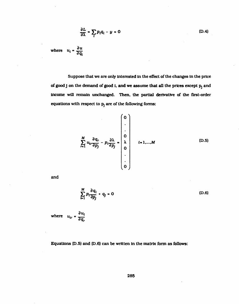
* !£ •* IZ p & i - y = 0 (D.4)

where u t du7qt

Suppose th a t we are only in terested in the effect o f the changes in the price

o f good j on the demand o f good 1, and we assume th a t a ll the prices except pj and

incom e w ill rem ain unchanged. Then, the p a rtia l derivative o f the firs t-o rd e r

equations w ith respect to pj are o f the fo llow ing form s:

'o '

M 3<Jr „ ax h u<r3 p ;" PlW j

0X0

v0 /

i- 1 .....M (D.5)

and

t- i(D.6)

where u*rd u t

W r

Equations (D.5) and (D.6) can be w ritte n in the m a trix form as follow s:

285

(U ir -P ] -P* 0

' 0 >

Bqt y 0"3J j X

d \B 0

7 p jJ J •

0-Q j\ J J

r « l.....Af (D.7)

Solving fo r E quation (D.7) gives

dqtSpj

(D.8)

and

dqt~**U m+1

(D.9)

where Sy is the elem ent (iJ) o f the inverse o f the m a trix on the le ft-hand side o f

E quation (D.7).

Thus, the S lu tsky sym m etry fo r the in d iv id u a l can be w ritte n as follow s:

Xs - d<ll + a d<it = dQ-> ♦ a dqJ = Xs XSV " Spj 9->7y Sp, q‘7y *SJ‘(D.10)

since Sy = Sjt.

We now tu rn to the sym m etry fo r m arket demand. The sym m etry o f m arket

dem and means

dQt &Qj dQj Spj °J~Sy W t l~3u

(D .li)

N Nwhere Qt « £ (q t)fc and Q j m (Qj)k 3116 m arke t demand fo r good i and j.

286

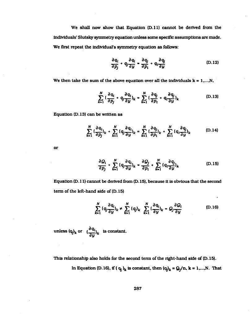
We sh a ll now show th a t E quation (D .ll) cannot be derived from the

in d iv id u a ls ’ S lu tsky sym m etry equation unless some specific assum ptions are made.

We firs t repeat the in d iv id u a l’s sym m etry equation as follow s:

bqt dq. Bq. , ,_ __ + + qt-^L ID . 12)Tpj 7pt Hl̂ y

We then take the sum o f the above equation over a ll the in d iv idua ls k = 1.....N ,

E quation (D. 13) can be w ritte n as

N dq, N dq, N 3q< ^ dq, ^ i

ID 1 4 ’

o r

E quation (D. 11) cannot be derived from (D. 15), because it is obvious th a t the second

term o f the le ft-hand side o f (D.15)

unless (qt)k o r (£ ? f). is constant. J dy K

T h is re la tionsh ip also holds fo r the second term o f the righ t-hand side o f (D. 15).

In E quation (D. 16), if ( qj )k is constant, then (qj)k = Q j/n , k = 1 .....N . That

287

is , a ll in d iv idua ls have the same am ount spent on good J. On the o ther hand, if

{dqt /d y )^ is constant, then a ll ind iv idua ls have the same shape o f Engel curve

fo r good 1. Since these tw o assum ptions are clearly inappropria te , the S lu tsky

sym m etry, in general, does not hold fo r m arket demand.

288

SELECTED BIBLIOGRAPHY

1. A lm on, C. (1979), "A System o f Consum ption Functions and its E stim ation fo r Belgium ," Southern Econom ic Jou rna l. V ol.46, pp. 85-106.

2. A lm on, C. (1988), The C raft o f Econom ic M odeling. Needham H eights, MA: G inn Press.

3. B lunde ll, C. (1988), "Consum er B ehavior Theory and E m pirica l Evidence - A Survey." Econom ic Jou rna l. Vol. 98, pp. 16-65.

4. B arten, A. P. (1977), "The System o f Consum er Demand Functions Approach: A Review," Econom etrica. Vol. 45, pp. 23-51.

5. Brow n, J . A. C. and A. S. Deaton (1972), "M odels o f Consum er Behavior: A Survey." Econom ic Jo u rn a l. Vol. 82. pp. 1145-1236.

6. Deaton, A. S. and J . M uellbauer (1980a), "An A lm ost Ideal Demand System ," Am erican Econom ic Review. Vol. 70, pp. 312-326.

7. Deaton, A . S. and J . M uellbauer (1980b). Econom ics and Consum er Behavior. Cam bridge: Cam bridge U n iversity Press.

8. Devine, P. (1983), "Forecasting Personal C onsum ption Expenditures w ith Cross-Section and Tim e Series D ata," U npublished Ph.D. D issertation, U n iversity o f M aryland, College Park.

9. Gauyacq, D. (1985), "Les Systemes Interdependants de Fonctions de Consom m ation," Prevision et Analyse Econom iaue. Vol. 6, No. 2.

10. M addala, G. S. (1983), L im ited Dependent and Q ua lita tive Variables in Econom etrics. Cam bridge: Cambridge U n iversity Press.

11. Nolan, B. (1987), Incom e D is trib u tio n and the Macroeconomv. Cam bridge: Cam bridge U n iversity Press.

12. P rais, S. J . and H. S. H outhakker (1955), The A nalysis o f Fam ily Budgets. Cam bridge: Cambridge U n iversity Press; 2nd ed ition , 1971.

13. Pollock, S. H. (1986), 'Incom e Taxes In a Long-Term M acroeconom etric Forecasting M odel," U npublished Ph.D. D isserta tion, U n iversity o f M aryland, College Park.

289

CURRICULUM VITAE

Name: Chang-yu I. Chao

Perm anent address: 9824 W ilden LaneR ockville, M aryland 20854

Degree and date to be conferred: Ph.D ., 1991

Date o f b irth : O ctober 2, 1959

Place o f b irth : Taipei, Taiwan

Secondary education: G irl’s F irs t Senior H igh School o f Tainan,Tainan, Taiwan

Collegiate in s titu tio n s attended:

In s titu tio n Dates o f A ttended

N ational Chiao-Tung U n iversity 1977-1979

N ational Taiwan U n iversity 1979-1982

U n iversity o f M aryland 1983-1986

U n iversity o f M aryland 1986-1991

M a jo r Econom ics

Professional positions held:

.Teaching A ssistan t, August 1984 - August 1989, D epartm ent o f Econom ics, U n iversity o f M aryland, College Park, M aryland.

.Load Forecast A nalyst, September 1989 - February 1991, Potomac E lectric Power Company, 1900 Pennsylvania Ave. NW, W ashington, D.C.

.Senior Load Forecast A nalyst, M arch 1991 - Present, Potomac E lectric Power Company, 1900 Pennsylvania Ave. NW, W ashington, D.C.

Degree Date o f Degree

B A . June, 1982

M A May, 1986

Ph.D. May, 1991