arX

iv:1

306.

6927

v2 [

astr

o-ph

.CO

] 1

1 A

ug 2

013

Emergent Cyclic Inflation, a Numerical

Investigation

William Duhe1 & Tirthabir Biswas2,

Department of Physics, Loyola University,6300 St. Charles Avenue

New Orleans, LA, 70118, USA

Abstract

We provide a comprehensive numerical study of the Emergent Cyclic Infla-tion scenario. This is a scenario where instead of traditional monotonic slow rollinflation, the universe expands over numerous short asymmetric cycles due tothe production of entropy via interactions among different species. This is oneof the very few scenarios of inflation which provides a nonsingular geodesicallycomplete space-time and does not require any “reheating” mechanism.

1wduhe@loyno.edu2tbiswas@loyno.edu

Contents

1 Introduction 1

2 Recycling the Universe 4

2.1 ECI, Motivation & Overview . . . . . . . . . . . . . . . . . . . . . . . 4

2.2 A prototype model . . . . . . . . . . . . . . . . . . . . . . . . . . . . 6

2.3 The NonRelativistic Case . . . . . . . . . . . . . . . . . . . . . . . . 8

2.4 Relativistic Case . . . . . . . . . . . . . . . . . . . . . . . . . . . . . 10

3 Entropy Production and Growth 13

3.1 Including the decay term & Back reaction from matter . . . . . . . . 14

3.2 Numerical Results . . . . . . . . . . . . . . . . . . . . . . . . . . . . . 16

4 Emergent Cyclic Inflation 18

4.1 Inflation . . . . . . . . . . . . . . . . . . . . . . . . . . . . . . . . . . 18

4.2 Emergence . . . . . . . . . . . . . . . . . . . . . . . . . . . . . . . . . 19

5 Summary and Future Directions 21

1 Introduction

The inflationary paradigm has been one of the cornerstones of success of the Standardcosmological model, for recent reviews see [1, 2]. However, the inflationary paradigmis incomplete in more than one way: While the slowly varying scalar potential energydriven inflation have been the favorite model, there have been a plethora of othermechanisms that has been considered in the literature, here are but a few examples [3–8]. Even within the general class of scalar field driven slow-roll inflation, models abidein plenty [1]. While the current observational data has been able to eliminate someof them, it is fair to say that we still don’t have any obvious winner among all theinflationary mechanisms/models. One can blame this lack of closure to our ignoranceof the “fundamental” particle/string theory but the inflationary space-time itself isalso “geodesically incomplete”. Essentially, if one tries to track a particle trajectoryinto the past, the geodesic ends abruptly at a finite proper time; and this has been

1

known since early days of inflationary cosmology 3 [12, 13]. It is clear that there hadto have been a “pre-inflationary” phase.

Naively it may seem that since the inflationary regime is an “attractor”, the pre-inflationary phase can simply be ignored without affecting any of the advantagesof inflation. Indeed, if one takes the view that the pre-inflationary phase was amonotonic expansion culminating in the past (possibly) in a quantum space-timeregime, which we are yet to understand fully, the arguments in favor of inflation seemrobust. However, as argued in [14], if instead one believes that an “effective space-time” description remains valid even at the Planckian era, and that the quantumgravity/stringy corrections are able to resolve the Big Bang singularity via the “BigBounce” 4 so that our phase of expansion is preceded by a phase of contraction,several advantages of the inflationary paradigm suddenly become questionable. Forinstance, if the Big Bounce is preceded by a long phase of contraction, the rapidgrowth of anisotropies as a−6 makes it very hard to imagine how the universe couldever have reached an isotropic patch where inflation could become activated; typicallylong before an FLRW bounce can be reached the universe would become completelyanisotropic entering into a chaotic Mixmaster phase [22, 23].

In this scenario it also becomes unclear why one should use the Bunch-Davisvacuum initial conditions for the calculation of the primordial spectrum of fluctuationsseeding the CMBR anisotropies. These calculations agree remarkably well with theobservations [24,25], but if one has a prior contracting phase, one ought to start withinitial seed fluctuations in that phase, track it through the bounce, and then alongthe inflationary expansion; there are no general arguments known to the authorswhich demonstrate that the resulting spectrum in such a case will still be nearlyscale-invariant as observed in CMBR. In fact, cosmologists have been looking atnon-inflationary mechanisms to generate the desired near scale-invariant spectrumutilizing the contraction/bounce phase, notable examples being the ekpyrotic [26],matter-bounce [27] and Hagedorn-bounce [28] scenarios.

In the presence of a bounce mechanism, to avoid these theoretical challenges aradically different inflationary mechanism was proposed in a series of articles [29–34]where one hopes to realize a geodesically complete non-singular inflationary paradigmvia a series of asymmetric short cycles. Here is the Emergent-Cyclic-Inflation (ECI)paradigm in brief:

• The universe “begins” in a quasi-periodic phase of oscillation around a finitesized universe. These oscillations continue all the way to past infinity becomingmore and more symmetric and periodic [29]. This is very similar to the “emer-gent universe” scenario advocated in [35, 36]. The potential energy is negative

3For other well known conceptual issues related to inflation see [9,10]. For a more recent criticismof the slow roll inflationary model in light of the latest results on the Higgs field coming from CERNsLarge Hadron Collider see [11].

4For quantum gravity/string theory inspired models which exhibit this property see for in-stance [15–21].

2

but it remains subdominant as compared to the negative curvature density as-sociated with a closed universe which cancels the matter densities to providethe turnarounds.

• This is followed by a phase of asymmetric cyclic growth when the negativepotential energy takes over from the negative curvature density in providingthe turnarounds. Over many cycles the space-time resembles the inflationarygrowth [31]. In every cycle (same time period) the volume of the universe growsby the same factor. This occurs because the entropy in each of these cycles dueto interaction between different particle species increases by the same factor.During this phase the magnitude of the curvature density is small as comparedto that of the cosmological constant.

• The cyclic inflation (CI) phase “graceful exits” via scalar field dynamics whichcan classically propels the universe from a negative to a positive potential energyregion, given the right “condition” [33] .

• Henceforth a monotonic phase of expansion begins as in the Standard Cosmolog-ical model. No reheating is required in the ECI paradigm as radiation remainsthe dominant energy density component throughout the entire evolution.

The ECI paradigm provides a nonsingular geodesically complete inflationary cosmol-ogy, does not require any reheating (which has it’s own challenges [2]), and inter-estingly predicts distinctive signatures in the form of small oscillatory wiggles in thepower spectrum [32] 5. It also provides new avenues of constructing phenomenologi-cally viable inflationary models where the initial potential energy could be negative.With the possible exception of the monopole problem the ECI can also address allthe old cosmological puzzles as in standard inflation.

While the cosmology described above was proposed and elaborated on in a seriesof papers [29–34], several arguments were either qualitative in nature or relied onnaive estimates. Our aim in this paper is to investigate the background cosmologyand test the viability of the ECI scenario comprehensively using numerical methods.In the process we also hope clarify the various parameter dependencies on observablefeatures in the CMBR spectrum, such as the amplitude and size of the oscillatorywiggles [32]. This would be useful when we try to fit the model to the recently re-leased Planck data using Monte Carlo simulations. Also, this is the first time when weexamine whether the “emergence” mechanism proposed in [29] meshes consistentlywith the cyclic inflation set-up 6. Finally, we provide a general framework to study

5There have been other cyclic models [37, 38] which also looked at the flow of perturbationsthrough various cycles.

6The scenario we will present here is similar to what was considered in [29], except that inECI one has a radiation dominated universe, where as in the set-up discussed in [29] the dominantcontribution to energy density came from the NR species. The importance of having a radiationdominated universe is that it’s pressure is able to avoid the Black-hole over-production problem,recurrent in cyclic cosmologies, see [31] for a detailed argument.

3

interacting thermal fluids in contracting backgrounds which may be useful in othercyclic/bouncing universe models which continues to be the most popular alternativeto the inflationary paradigm. For instance, through the course of our numerical in-vestigation we found that the naive estimate of the temperature at which thermalequilibrium can be restored in a contracting universe is a little lower than what ournumerical simulations show. On the other hand, once such an equilibrium is estab-lished, the various components (relativistic by now) continue to track the equilibriumdensities all the way up to Planckian bounce densities, even though it is well knownthat they should not be able to maintain thermal equilibrium at such high tempera-tures [39]. This is essentially the analogue of the phenomena that is observed in theexpanding phase involving the CMBR photons; the fact that they still obey Planck’sblackbody distribution even though they have been traveling essentially freely for thelast 14 billion years or so. This finding may be relevant for different cosmologicalscenarios: For instance, one of the criticisms [40] of the String Gas Cosmology frame-work [41] is that it is very difficult to establish thermal equilibrium among all thestringy excitations in the Hagedorn phase. Our analysis suggests that there may bea way around this problem if one includes a prior contracting phase.

Our paper is organized as follows: In section 2, we will first introduce a toy modelwhich can realize the CI mechanism and test whether after each turnaround it ispossible to recreate the nonrelativistic particles from the massless degrees of freedomin the contracting phase, and whether thermal equilibrium can be re-established.This is key in being able to sustain the inflationary growth over many cycles. Insection 3, we will look at the coupled dynamics of the massless and massive speciesalong with the scale factor in a given cycle, and track the growth of the scale factordue to entropy production. Next, in section 4, we will verify whether the universecan indeed sustain the inflationary growth over numerous cycles. We will also look atthe merging of the cyclic inflation scenario with the emergence mechanism [29]. Wewill conclude with a perspective on future research directions in section 5.

2 Recycling the Universe

2.1 ECI, Motivation & Overview

As argued in the introduction (also see [14]), if the universe has a built-in mechanismto bounce from a phase of contraction to a phase of expansion, some of the advantagesof the inflationary paradigm are lost (or at least need to be revisited). One way ofsalvaging the scenario is by relaxing the pre-condition that our universe “started” withpositive potential energy. Actually, there is yet no known “theoretical” reasons asto why the universe should have positive potential energy. String theory, the leadingcandidate for a consistent theory of quantum gravity, naturally predicts the existenceof negative energy vacua, and in fact, it has been quite a challenge to find ways thatmay lead to positive vacuum energies in the string theory framework [42]. The same

4

is also true for supergravity theories [43]. In general, if one looks at the potentialenergy coming from all the moduli in any fundamental theory, one would expectto have both negative and positive potential regions, and local minima’s dispersedliberally [44]. What we do know however from cosmological observations, is thatcurrently the universe has a positive cosmological constant [45]. We will see laterhow the ECI paradigm can reconcile this apparent contradiction between the earlyand late time cosmology.

Presently, let us try to investigate the dynamics of a “small” but relatively smoothpatch in the “Early Universe”with negative vacuum energy density, Λ < 0. Typically,with such a patch apart from the vacuum/potential energy, Λ, one expects to associateenergy density components such as spatial curvature, ρk ∼ a−2, massless degrees offreedom (radiation), ρr ∼ a−4, perhaps some massive modes as well, ρm ∼ a−3, andpossibly small amounts of anisotropies 7, ρa ∼ a−6. If |Λ| > ρr + ρm + ρk, FRWevolution is inconsistent, most likely the universe would be stuck in a static anti-deSitter like universe containing massless and massive excitations. Let us then look atthe opposite case when |Λ| < ρr + ρm + ρk. In this case, as the universe expands, allthe matter components would dilute and eventually cancel the negative cosmologicalconstant causing the universe to turnaround and start contracting. As the energydensity increases to Planckian densities, according to our prior assumption, quantumgravity effects would prevent a Big Crunch singularity and usher in the next phase ofexpansion. This story will keep on repeating leading to a cyclic model.

At first glance, such a cyclic universe is completely inconsistent with our universe.If |Λ| is large, given possibly by the string/GUT scale, typically a few orders ofmagnitude below the Planck scale, then each of the cycles would only last a very shorttime τ ∼ Mp/

√Λ ∼ 10−33 s, much too short for any realistic cosmology. Making |Λ|

small to allow for structure formation doesn’t help either because it will be in violentconflict with the current cosmic speed-up data. What turns out to be a naturalsavior is in any realistic high energy physics model one expects interactions betweendifferent particle species which tends to create entropy. Entropy can only increasemonotonically according to the second law of thermodynamics, this then provides asimple way of breaking the periodicity of the evolution. Actually, this was preciselywhat Tolman pointed out in the 1930’s giving rise to Tolman’s entropy problem forcyclic models [46, 47], but we can now use the entropy production to our advantage.As was first pointed out in [31], and will be further elaborated on in this paper,entropy tends to increase by the same factor in every cycle, while the time periodof the cycles remains a constant since it is governed by Λ (which for simplicity wewill assume to be a constant). This means that the universe must be growing by thesame factor in every cycle giving rise to an overall inflationary growth! Most of theadvantages of the standard inflationary paradigm rolls over to this scenario, includingthe production of near scale-invariant density fluctuations, see [14, 31, 32] for details.

7One could also add energy coming from kinetic energy of massless scalar fields, but it behavesin a manner very similar to that of the anisotropies, ρφ ∼ a−6, and therefore can be clubbed withρa.

5

As one must, with any inflationary mechanism, we need to provide a “gracefulexit”. In an expanding background it is known that energy densities of scalar fieldscan only decrease, and hence once the universe is in a negative energy phase, there isno way for it to claw back up to the positive region. However, in contracting phasesthe reverse is true i.e., the energy density increases, and in [33] (see also [48–51])it was demonstrated that contracting phases can indeed facilitate a transition fromnegative to positive potential energy regions. Thus our universe could have beeninflating while “exploring” the negative potential regions when at some point it madea classical jump to a positive potential energy region, in the process providing agraceful exit from the CI phase and ushering in an everlasting monotonic phase ofexpansion thereafter!

There is a final twist to the beginning of the story. Let us revisit the issue ofgeodesic completeness in the context of the CI scenario. If one tracks, say, the maxi-mum of the oscillating space time, then one finds that it has the traditional inflation-ary trajectory. The problem of past geodesic incompleteness comes back to haunt us!Fortunately, there may be a natural resolution for a closed universe 8. In this case, asone goes back in cycles there comes a point when the negative curvature energy den-sity becomes more important than the negative vacuum energy density. (Curvaturedensity blue shifts as a−2, while the vacuum energy density remains a constant.) Oncethis happens, the universe no longer turns around due to the negative vacuum energydensity, but before, when ρr + ρk = 0. The temperature of the turnaround increasesmaking the universe spend less and less time in the out-of-equilibrium phases (mas-sive particles only fall out-of-equilibrium when their temperature falls below theirmasses). This ensures that the entropy increase becomes less and less as we go fur-ther back in cycles, and eventually the universe asymptotes to a periodic evolutionas t → −∞. The space-time is, in fact, very reminiscent of the emergent universescenario advocated in [35,36], and this is reason why refer to our cosmological modelas “emergent-cyclic-inflation” or ECI.

2.2 A prototype model

To illustrate the basics of the CI mechanism it is sufficient to consider a universewhere we have a negative cosmological constant 9 (−Λ), and the “matter content”of the universe consists of a single non-relativistic (NR) species, ψ, along with rela-tivistic degrees of freedom, collectively denoted by X . To obtain the cyclic evolution,we will assume that during contraction when a critical Planckian energy density, ρ•,is reached, the universe bounces back nonsingularly to a phase of expansion. While

8The model only works if the universe is closed. For an open patch, one ends up with a verydifferent dynamics and an universe nothing in common to ours.

9The evolution of Λ as a function of the various scalar fields that may be present in a fundamentaltheory is only relevant in the discussion of the spectral tilt, as Λ controls the amplitude of theprimordial spectrum, and in the discussion of the graceful exit mechanism from the CI phase. Theseissues have been addressed in [32] and [33], but we plan on performing a comprehensive numericalanalysis that will be required when we fit our model to the Planck data.

6

the Big Bounce is still very much a conjecture, and there is yet to be a completelyconvincing mechanism in place, several different bouncing mechanism have been con-sidered in the literature, and in many of these models a bounce occurs when the energydensity reaches close to the Planck density, see for instance [15–18, 52–55]. For thepurpose of our paper we will simply assume the existence of such a mechanism, whatwill become evident is that the details of the mechanism of the bounce are not goingto be particularly important for our model, and this is clearly an advantage.

Away from the bounce when GR is valid, the Hubble equation corresponding toflat Friedman-Lemaitre-Robertson-Walker (FLRW) cosmology reads

H2 =ρ

3M2p

, (2.1)

where ρ is the total energy density given by

ρ = ρm + ρr − Λ . (2.2)

where ρm and ρr corresponds to the energy density associated with ψ and X . Now,in an expanding phase the total “matter” density (ρr + ρm) dilutes, and eventuallyit is canceled by the potential energy, −Λ, as H → 0 signalling a “turnaround” toa contracting phase. Thereafter, the matter energy density increases with increasingtemperature and eventually when it reaches ρb, the universe transitions to the expand-ing branch of the next cycle according to our assumption of the Big Crunch/Bangtransition. This then provides us with a cyclic model with a time period of oscillationapproximately given by [29] 10.

T ≈√3πMp

2√Λ

. (2.3)

The mechanism to obtain inflation in this scenario exploits entropy productionwhen ψ and X interacts. The idea is the following, if m is the mass of ψ, then ψparticles are expected to remain in thermal equilibrium with X as long as T & mvia scattering processes. Below T = m, the massive ψ particles, which are now non-relativistic, will fall out of equilibrium, and consequently if and when they decay intoradiation thermal entropy will be generated. This will cause the universe to grow bymaking the cycles slightly asymmetric. After the turnaround, once the temperaturebecomes sufficiently high, the massive particles are expected to be recreated fromradiation via the scattering processes re-establishing thermal equilibrium before thenext cycle commences. In order to sustain this growth over many many cyles, whatthen becomes crucial is to check whether in the contracting universe when the tem-perature rises above T = m, the scattering processes can indeed recreate ψ from Xallowing equilibrium to be re-established between NR matter and radiation. Whilenaive arguments by comparing the Hubble rate with scattering rate suggests that thisshould happen [31], we want to test this assumption first.

10In the derivation of the time period it was assumed that the matter density is always dominatedby radiation.

7

Now, the NR particles are expected to decay into massless degrees during theexpansion phase prior to the turnaround, let us in fact consider the case when noneof these particles are left at the onset of the contraction phase. To keep the physicssimple, we are going to ignore the backreaction of the NR particles on the Hubbleexpansion rate in this section. It is only going to be relevant for the study of entropyproduction that we will investigate in the next section.

Let us consider some gauge mediated creation/annihilation processes between ψparticles and X :

ψ + ψ ↔ X +X . (2.4)

What we want to address is really the inverse of the relic/dark matter density compu-tation in conventional Big Bang cosmology. In that case, we start by assuming thatall the species are in thermal equilibrium with each other and ask when the massivespecies decouples. Here we are going to start by assuming that the ψ particles are notin equilibrium with X , and ask whether the scattering processes can recreate themto equilibrium densities.

The Boltzman equation corresponding to simple processes like (2.4) reads [39]

n+ 3Hn =< σ|v| > [n2 − n2] , (2.5)

where n is the number density of the ψ particles, and n is the equilibrium numberdensity given by

n =1

2π2

∫

∞

m

√ǫ2 −m2

eǫT ± 1

ǫ dǫ =T 3

2π2

∫

∞

m/T

√

y2 − (m/T )2

ey ± 1ydy ≡ T 3β(T/m) (2.6)

< σ|v| > is the average cross-section times relative velocity for the process (2.4), andis typically a function of the temperature. If we know < σ|v| >, in principle (2.5) canbe solved in conjunction with the Hubble equation and the Boltzman equation for X .

2.3 The NonRelativistic Case

We will first focus on the nonrelativistic limit, T < m, to illustrate the re-equilibriation process as most of the relevant quantities have simple analytic forms inthis regime. For the nonrelativistic limit we have

n =

(

mT

2π

)3/2

e−m/T , (2.7)

while on general theoretical considerations the thermally averaged < σ|v| > is ex-pected to go as a power of |v| ∼

√

T/m. It can thus be parameterized as

< σ|v| >= σ0

(

T

m

)n

. (2.8)

8

For instance, for the s wave channel n = 0, and for p wave, n = 1 [39]. We willnumerically analyze both these cases. σ0 characterizes the strength of the interactionand would, for instance, be proportional to the square of the appropriate gauge finestructure constant.

According to the usual lore, we expect equilibrium to be established when theinteraction rate, Γs = n < σ|v| >, catches up with the Hubble expansion rate, H ,given by

H2 =ρr

3M2p

=gπ2T 4

90M2p

. (2.9)

Above we have used the approximation that at the equilibrium temperature, the uni-verse primarily contains massless particles, g being the number of “effective” bosonicdegrees of freedom. Then the condition for re-establishing thermal equilibrium isgiven by

Γs = σ0

(

mT

2π

)3/2

e−m

T

(

T

m

)n

≈√

gπ2

90

T 2

Mp(2.10)

Defining a new variable x ≡ T/m, we can implicitly find the xmin (or equivalentlythe temperature) above which equilibrium can be maintained:

exp( 1

xmin)√xmin

xnmin= Aα where A =

3

2π2

√

5

π, (2.11)

and

α ≡ σ0mMp√g

(2.12)

is the combined dimensionless parameter on which xmin solely depends.

We are now going to study the process numerically. Substituting (2.8) in (2.5) wehave

n+ 3Hn = σ0

(

T

m

)n(

n2 − n2)

. (2.13)

Expressing the time derivative in terms of the temperature derivative, and using (2.9)and the fact that T ∝ 1/a in radiation dominated universe, we obtain a reasonablysimple equation for the dimensionless variable β ≡ n/T 3:

dβ

dx= α

√

90

π2xn(β2 − β2) , (2.14)

We had previously chosen β in such a way that β ≡ n/T 3.

In the NR limit we have

β(x) =e−

1

x

(2πx)3/2(2.15)

To keep track of the departure from equilibrium let us define the ratio

R ≡ n

n=β

β(2.16)

9

From our numerical analysis, see Fig. 1, it is clear that the scattering processesare indeed efficient enough to produce the ψ particles from radiation and establishequilibrium densities. Fig. 1 also shows that the larger the value of n the longerit takes (higher the temperature) for equilibrium between the NR and relativisticparticles to be established; this is to be expected as larger value of n means smallerinteraction rate for x < 1 and hence the longer time-scale needed.

In Fig. 2 we have plotted the numerically obtained equilibrium temperature as afunction of α by solving (2.14) in conjunction with the naive estimate given by (2.11).Firstly, it is clear that the more one increases α, the faster one reaches equilibriumi.e. , equilibrium is reached at smaller values of x (temperature). This is obviouslywhat one expects and the general trend agrees with the naive estimate (2.11) basedon comparison of scattering and Hubble rate. We do note in actuality it takes a littlelonger to establish thermal equilibrium between ψ and X than the naive estimate(2.11), but the discrepancy is within the order of magnitude.

0.1 0.2 0.3 0.4 0.5 0.6 0.7x

0.2

0.4

0.6

0.8

1.0

R

0.1 0.2 0.3 0.4 0.5 0.6 0.7x

0.2

0.4

0.6

0.8

1.0

R

Figure 1: Equilibrium being reached at varying values of α ranging from 500 to 15000 in steps of

500. Left: n = 0; Right n = 1.

2.4 Relativistic Case

While there are no phenomenological or theoretical hindrances in looking into theevolution when the ψ particles become relativistic, there are no closed form resultsfor the integral appearing in the equilibrium number density (2.6) spanning the entiretemperature range. Therefore if one were to incorporate it exactly, one would needto solve integro-differential equations which are numerically much more challengingand requires significantly more computational time. Fortunately, we have found anexcellent approximation (within a percent) to (2.6):

β(x) ≈ e−1

x

(

1.68512 + 1.94285x−0.84331 − 0.72446x−1 +

√

π

2x−3/2

)

(2.17)

10

-7 -6 -5 -4 -3 -2 -1

1

2

3

4

5

6

7

1000 2000 3000 4000 5000

0.1

0.2

0.3

0.4

0.5

Figure 2: Left: A comparison between the exact numerical expression of the thermal number

density given by (2.6) and the approximation given by (2.17). The horizontal axis corresponds to

the natural logarithm of m/T . We see that almost up to m/T ∼ O(10−3) the approximation is

very good. Right: the A plot of xeq = Teq/m as one changes α. The red dashed line represents the

curve based on the naive theoretical expectation given by (2.11), the blue line corresponds to the

numerical value using the Non-relativistic approximation (2.7) while the green line corresponds to

the numerical value using the more accurate approximation formula (2.17) and p = 0.1.

which can be used for the temperature range x < 103 and is sufficient for our pur-pose 11. Fig. 2 (left) shows a plot of the exact numerical evaluation vs the approximateanalytical function we are using.

0 5 10 15 20x0.0

0.2

0.4

0.6

0.8

1.0R

0.2 0.4 0.6 0.8 1.0 1.2 1.4x

0.2

0.4

0.6

0.8

1.0

Figure 3: Left: A plot of xeq = Teq/m with α = 1 . . . 200 in interval of 5 and p = 0.1. Right: The

orange curve represents plots of the scattering cross-section with p = 0.1 . . .1 in intervals of 0.1. The

smaller the value of p, the sharper is the transition from the NR to the relativistic regime. The red

curves provides the corresponding plot for R(x) as one changes p.

We also need to modify the scattering cross-section (2.8) that we used for thenon-relativistic regime. In the relativistic regime, if the interactions are mediated by

11In the CI model the amplitude of the power spectrum is proportional to Λ3/4/M3

p [34]. Therefore

to obtain the observed value of around 10−10, one requires Λ1/4 ∼ 10−3Mp and since in our modelthe variation of the temperature and the mass is limited to Mp & T,m & Λ1/4, the range x . 103

covers most of the relevant parameter space.

11

massless (light) gauge bosons, the cross-section is expected to go as [39]:

< σ|v| >= σr

(m

T

)2

(2.18)

where σrm2 ∼ α2

f, αf being the relevant fine structure constant. Now, the details ofhow the scattering crosssection transitions from it’s nonrelativistic expression (2.8)to the relativistic one (2.18) depends on the specific high energy physics model inquestion. Here we will take a phenomenological approach to parameterize the cross-section as

< σ|v| >= σ0[

1 + (3x)2

p

]p ≡ σ0s(x) (2.19)

For x ≪ 0.33 we recover the constant n = 0 non-relativistic cross-section, while forx ≫ 0.33, the expression approaches the relativistic approximation with σr = σ0/9,just a convenient choice to keep the number of parameters tractable. The parameterp controls how fast the transition is from the non-relativistic to the relativistic regime,see Fig. 3, right. The equation we need to solve is then a simple generalization of thenon-relativistic version

dβ

dx= α

√

90

π2s(x)(β2 − β2) , (2.20)

where β(x) is now given by (2.17).

Before we go on to study the numerics, let us review some of the well known resultspertaining to thermal equilibrium in relativistic species. Since in the relativisticregime (2.18) the interaction rate goes as

Γs ∼ n < σ|v| >∼ T 3σr

(m

T

)2

,

equating this with the Hubble parameter one finds that the condition for maintainingthermal equilibrium is given by

T

m.σrmMp√

g=α

9≡ xmax (2.21)

where we have used the simple relation that exists between σr and σ0. So at least inour specific case, the same parameter α that controls the temperature at which equilib-rium is reached, also controls the maximum temperature up to which the equilibriumcan be maintained 12. What we found however was that even when the temperatureswere way larger than this maximal equilibrium temperature, the ψ density hardlydeviates from the equilibrium density, see Fig. 3 (left). In hindsight, this shouldnot have come as a surprise as it is well known that once a massless species attainsequilibrium, the equilibrium densities are automatically maintained even when the

12In general if the dominant scattering process responsible for maintaining equilibrium betweenψ and X in the relativistic and NR regime, then the parameters controlling the minimum andmaximum temperatures for equilibrium will be different.

12

excitations are no longer interacting with each other. This is precisely the reasonwhy the CMBR still agrees so well with the Planckian distribution. Thus, it turnsout that for the cyclic inflation model, it doesn’t make any difference whether theequilibrium is technically lost at some high temperature or not; as long as equilib-rium was established at some temperature in the contracting universe, equilibriumdensities are maintained till the beginning of the next cycle. This adds robustness tothe CI mechanism. In general we do not find too much of a difference between thetemperatures when equilibrium is reached when we use the NR approximation (2.7)as opposed to the more exact numerical approximation (2.17)

Our numerical analysis also provides a lower bound for α, below which thermalequilibrium is never attained. For instance, p = 0.1 at α = 70, one only attains 90%of the equilibrium density. As we decrease α further, the maximum ratio R attainedgoes down further. At α = 0.1, this ratio is only 0.005. What is interesting is theratio remains essentially a constant as the temperature increases towards the bounce,and will essentially be the same for every cycle, see Fig. 3 (left). Thus the periodicityin energy density of the different species can still be maintained over numerous cycleswhich is the main ingredient needed for CI mechanism. The CI mechanism appears,clearly, to be more robust than previously thought. Now, the smaller the ratio Rthat can be achieved, the smaller the entropy production, and therefore the slowerthe inflationary growth and eventually this will make the scenario unviable 13. Onthe other hand, if α is too large this would correspond to an entropy increase thatwould lead to large oscillations in the CMBR spectrum that we don’t see [32]. Inshort, CMBR can be used to constrain a particle physics parameter such as α, butthese issues are left for future considerations.

3 Entropy Production and Growth

In the earlier section we saw that, even if we started with no ψ particles, theycould be recreated and thermal equilibrium with radiation could be established asthe temperature rose in the contraction phase. What we did not discuss is how the ψparticles are removed from the system in the first place. The idea, simply, is to makethe ψ particles unstable and include decays of ψ into X . Such a decay term, in fact,is absolutely crucial for the success of the CI mechanism, as it is responsible for theproduction of entropy, which manifests itself in the asymmetry of the cyclic evolutionleading to a small growth of the scale factor in any given cycle. In this section we wantto analyze the entire thermodynamic evolution involving the ψ particles. We wantto see how they first fall out of equilibrium during expansion and subsequently decaycreating entropy and then finally how they are re-created during contraction. In the

13In the analysis done in [32], the optimal entropy production favored by the data seems to be afactor of around 1.005, such fits with the CMBR data would in principle, impose a constraint on howsmall or large an α may be phenomenologically favorable. Moreover, having a very slow inflationarygrowth would imply that Λ(φ) would have to remain small for a very long time, thereby increasingthe fine-tuning problems that are associated with flatness of potentials in inflationary models.

13

process we will also determine whether the universe indeed grows in a given cycle ashas been argued, and if so, then how does this growth depend on the parameters ofthe model.

In order to investigate this story we will need to incorporate the decay term,include the backreaction of the NR species on the expansion of the universe, andtrack β as a function of time rather than temperature as we want to include boththe expanding and the contracting branches. To keep things tractable we will nowspecialize to the case when ψ particles always remain non-relativistic, this can beachieved by choosing m & ρ

1/4• , then even at the bounce the temperature is less than

m.

3.1 Including the decay term & Back reaction from matter

It is relatively straight forward to include the decay term. In the presence of a processsuch as

ψ → X +X (3.22)

we need to add a decay term in the continuity equation (2.5) for ψ:

n+ 3Hn = −Γdn+ < σ|v| > [n2 − n2] , (3.23)

where Γd, the decay rate is a constant and depends on the details of the specificparticle physics processes. An equation for ρm can be obtained straight forwardly bysimply multiplying (3.23) by m:

ρm + 3Hρm = −Γdρm +σ0m

(

T

m

)n

[ρ2m − ρ2m] , (3.24)

Notice, we have switched from using β(t) variable to ρm(t) for transparency. ρm isjust the equilibrium matter density given by

ρm = mn = mT 3β (x) (3.25)

(3.24) needs to be solved in conjunction with the Hubble equation (2.1). Actually,the Hubble equation is not the best choice to perform numerical calculations involvingtransitions from expansions and contractions, as one would then need to manuallychange the sign of the square-root. The way around this technical problem is to usethe Raychaudhury equation

a

a= − 1

6M2p

(ρtot + 3ptot) = − 1

6M2p

(

gπ2

15T 4 + ρm + 2Λ

)

(3.26)

along with the initial conditions given by the Hubble equation.

Finally, we also need an equation for the temperature. This is given by

T +HT =15Γdρm2gπ2T 3

− 15σ02gπ2T 3m

(

T

m

)n

[ρ2m − ρ2m] (3.27)

14

The easiest way to obtain the above is to realize that the total stress energy tensormust be conserved. One can of course obtain the same equation directly by incorpo-rating the interaction terms in the continuity equation for radiation.

Before solving the equations (3.24), (3.26) and (3.27) numerically, let us lookat the parameters controlling the physics of the evolution. Naively, there are sixparameters, Mp, m, σ0, g,Λ and Γd. However, we know that the asymmetry in thecyclic evolution of the universe is produced as a result of the out-of-equilibrium decayof the massive particles. Such decay processes are only initiated once temperaturefalls below the equilibrium temperature, and therefore will be governed by α, see theprevious section. Clearly, the amount of entropy generated should also depend on thedecay rate, or Γd, as that controls the entropy production rate. Finally, it should alsodepend on the amount of time that is available for the decay processes to occur whichis dictated by the time period of the cycle, T (2.3). Thus, on physical grounds weexpect the growth in entropy/scale-factor to be dictated only by three independentparameters. Indeed, this becomes manifest if we re-write equations (3.24-3.27) byrescaling some of the variables:

ρm = gm4R (3.28)

t =

(

Mp√gm2

)

τ (3.29)

The above rescaling has a rather simple interpretation; gm4 is approximately theenergy density of radiation at the time the massive species becomes non-relativistic.Essentially we are measuring the energy densities in units of this density, and time inunits of the time when this transition occurred. In terms of these new variables theequations look

a′′

a= −1

6

(

π2

15x4 +R + 2λ

)

(3.30)

R′ + 3R

(

a′

a

)

= −γR + gαxn[R2 − R2] (3.31)

x′ + x

(

a′

a

)

=15γR

2π2x3− 15gα

2π2xn−3[R2 −R2] (3.32)

where the set of relevant dimensionless parameters are given by

γ ≡ MpΓd√gm2

(3.33)

λ ≡ Λ

gm4, (3.34)

and the combination gα. We have also defined

R =ρmgm4

=x3

gβ (x) , (3.35)

15

as one can guess. Again, we are simply measuring Λ and Γd in terms of the units as-sociated with the transition of the massive species from relativistic to non-relativisticregime.

3.2 Numerical Results

200 400 600 800Τ

2

4

6

8

10

12

R

2000 2200 2400 2600 2800 3000α

0.0085

0.0090

0.0095

0.0100

0.0105

Change in aHtL

0.002 0.004 0.006 0.008 0.010Γ

0.0082

0.0084

0.0086

0.0088

0.0090

0.0092

Change in aHtL

Figure 4: Left: The blue curve tracks R. It starts out at one and after the turnaround, again

inches back up to one. The red curve is a plot of the scale factor around the turnaround. The

other two figures show how the growth of the scale factor changes with the parameters of the model.

Center: Variation with α, Right: variation with γ.

Since the nonrelativistic limit is only valid as long as 3T < m, we start ournumerical simulations from x(0) = 0.33. The initial condition for R can be imposedstraightforwardly, R(0) = R(x = 0.33) i.e. we start our simulation with equilibriumdensities. We can also set a(0) = 1 as a convention. The initial derivative is thenconstrained according to the Hubble equation:

(

a′

a

)2

=1

3

(

R +π2

30x4 − λ

)

(3.36)

Also we choose g = 1 in all the following simulations.

Fig. 4 is perhaps the best testament to the viability of the CI scenario. We startwith equilibrium density so that the ratio R is one. Very quickly, ψ falls out of equi-librium, so it starts to behave like NR matter, diluting more slowly (∼ a−3) thanit would if thermal equilibrium was maintained (the Boltzman exponential suppres-sion would then be taking over). This is reflected in the R > 1 values. This trendcontinues till we reach the decay time scale at which point all the ψ particles decayinto radiation, generating entropy in the process. Finally, in the contracting phasewhen the temperature rises again the scattering processes are able to replenish theψ particles back to equilibrium values. This is exactly what was argued should hap-pen in [29–31], but it is reassuring to verify the mechanism keeping track of all theinteractions and back-reactions.

Fig. 4 shows plots of how the universe grows during this process as we vary therelevant parameters. The graph at the center exhibits a monotonic decrease in thegrowth as we increase α. This is easy to understand: as α increases the universe

16

is able to maintain thermal equilibrium for a longer time and hence the “out ofequilibrium-ness” when the ψ particles do decay becomes less, and in return lessentropy is produced. If α is so large that ψ is never out of equilibrium, the evolutionwould be completely symmetric and no entropy would be generated at all.

In Fig. 4, the graph on the left shows how the growth is affected as we vary thedecay rate and it is a bit more interesting. Initially the growth increases with theincrease of the decay rate, and this is obvious. If there is no decay, there is no entropygeneration, and as the decay time shrinks the entropy production increases. However,once the decay time scale becomes shorter than the time period, we also start to seea decrease in the growth. This is because, if the ψ particles decay too quickly, theyare not sufficiently out of equilibrium when they decay. If in fact the decay time scalebecomes smaller than the scattering time scale, we again won’t generate any entropy.This is what is represented in the graph.

Before ending this section, let us emphasize that although we used entropy argu-ments to explain the various features of our numerical results, one could also explaineverything in terms of the asymmetry in the NR-matter content between the expand-ing and contracting phases. In this language the reason why the universe grows a bitmore in the expanding branch than it contracts during contraction is because in theformer there is a bit more NR-matter than the latter phase, and the universe expands(or contracts) faster in presence of matter than radiation (t2/3 as opposed to

√t).

To summarize, we have verified through the course of a cycle (really theturnaround) the interactions between the NR and radiative degrees of freedom canproduce entropy which causes the universe to expand slightly. We also found the waythe growth depends on some of the relevant parameters such as the scattering interac-tion strength, the decay time and the cycle period, controlled by α, γ, λ respectively,were along the expected physical arguments. Although for technical reasons 14 weperformed our analysis in the NR regime, we do not expect any qualitative changesif we were to include relativistic regimes. In passing we also note that the optimalvalue of entropy increase, a factor of around 1.005, that was found while fitting theWMAP data [32] is easily obtainable from the model parameters, see Fig. 4 (centerand right).

14We would not only have to use the approximation (2.17) for the number density of ψ, we wouldhave also had to account for the fact that the number and energy densities are no longer simplyrelated through a constant mass, m, but rather through some complex temperature dependentfunction. Moreover, this would make the equations in terms of energy densities for ψ andX extremelycumbersome, without giving us any new physical insights.

17

4 Emergent Cyclic Inflation

4.1 Inflation

Having seen how the universe can undergo asymmetric cycles it is time to provide asimulation involving many cycles where we can observe the exponential inflationarygrowth. In order to achieve this we need to include a last ingredient in our model, abouncing mechanism. We chose to model the bounce using a ρ2 type correction thathas been suggested in Loop Quantum gravity literature [15,16] as well as some modelsinvolving brane physics [17]. We would like to emphasize, that our primary motivationfor choosing this correction is purely technical, it is easy to implement numerically.The details of the bouncing mechanism doesn’t affect any of our arguments as they arehappening at temperatures much smaller than the bounce temperature, see [18,19,55]for some of the other bouncing mechanisms that has been proposed in the literature.According to the ρ2 bounce the Hubble equation is modified as

H2 =ρ

3M2p

(

1− ρ

ρ•

)

(4.37)

As before, for numerical purposes we have to work with the modified Raychaudhuryequation:

a

a= − 1

M2p

[

1

6(ρ+ 3p)− ρ

ρ•(3p+ 2ρ)

]

(4.38)

Here ρ and p refers to the total energy density and pressure:

ρ = gT 4 + ρm − Λ (4.39)

p =1

3gT 4 + Λ , (4.40)

and ρ• is the energy density at which the universe bounces from a contracting to anexpanding phase as is obvious from (4.37).

In terms of the rescaled variables the equation reads

a′′

a= −

[

1

6

(

π2

15x4 +R + 2λ

)

− κ

(

π2

30x4 +R− λ

)(

π2

10x4 + 2R + λ

)]

(4.41)

where

κ ≡ gm4

ρ•(4.42)

The appropriate initial condition is given by

(

a′

a

)2

=1

3

(

R +π2

30x4 − λ

)[

1− κ

(

R +π2

30x4 − λ

)]

(4.43)

18

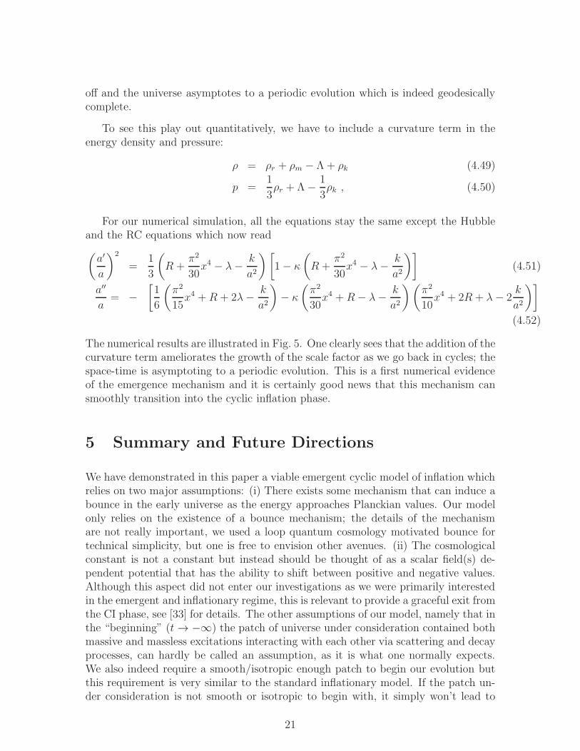
Fig. 5 shows the evolution of the scale factor over numerous cycles. Evidently, theevolution shows an exponential growth over many cycles. Indeed the cyclic inflationmechanism works!

We noticed that while the turnarounds smoothly increases as an exponential, thebounce points are a bit more irregular, although on an average, they also continueto increase exponentially. This is essentially because small differences in the ratio ofmatter/radiation in different cycles can have a relatively large effect on the size of theuniverse at the bounce 15. In any case, for the CI paradigm what is more importantis the turnaround scale-factor as the fluctuations freeze near the turnarounds. It isthis energy scale that is important for the reproduction of the near scale-invariantspectrum. We also note that since both the turnaround and the bounce increase, sodoes their difference, as is evident on the graph.

Finally, we would like to re-emphasize that this cyclic behavior needs to cometo an end and usher in a stage of monotonic expansion. This is indeed possible ifone upgrades the cosmological constant to the potential energy coming from variousscalar (moduli) fields, the scalar field can then roll along a relatively flat negativepotential energy region before making a classical jump to a positive energy regionwithin a single contracting phase. This happens for quite natural initial conditionsand have been studied in [33]. We therefore do not elaborate on this mechanism here.

50 000 100 000 150 000 200 000 250 000 300 000Τ

10

20

30

40

50

60

a

2000 4000 6000 8000Τ

1

2

3

4

5

a

100 000 200 000 300 000 400 000Time

50

100

150

aHtL

Figure 5: Left: Exponential Growth over many cycles. Center: We have zoomed in to see how

the growth occurs over a few consecutive cycles. Right: The evolution in red again corresponds to

the cyclic inflationary growth as exhibited by the plot on the left, but the plot in blue corresponds

to the evolution for a closed universe. It is clear that the universe, in this case, asymptotes to a

periodic evolution in the past.

4.2 Emergence

Let us finally revisit the issue of geodesic completeness in the context of the CIscenario. One of the main theoretical benefits of the CI model as compared to the

15We also note that the differences between the consecutive bounce points somehow seem a bitlarge when looking at plots including many cycles such as Fig. 5 (right), this is actually a plottingerror. When one zooms into a few cycles as the Fig. 5 (center), these discrepancies mostly go away.

19

traditional inflationary scenario is that it is nonsingular and can be extended into theinfinite past. But is that really true? If one tracks, say, the maxima/turnaroundsof the oscillating space time, then one finds that it has the traditional inflationarytrajectory, so the problem of past geodesic incompleteness apparently comes backto haunt us! Fortunately, there appears a natural resolution for a closed universemodel which was first put forward in [29] in a slightly different setting: As one goesback in cycles, there comes a point when the curvature energy density becomes moreimportant than the vacuum energy density. (Curvature density blue shifts as a−2,while the vacuum energy density remains a constant.) Once this happens, the universeno longer turns around due to the negative vacuum energy density, but before, whenρr + ρk = 0. Let us then look at the dependency of the turnaround temperature onthe entropy S of the universe. A convenient choice for the scale factor and the metricis given by [23]

ds2 = −dt2 + a2(t)

(

dr2

1− kgm4r2/3M2p

+ r2dΩ2

)

and a = g1

4mV 1/3 (4.44)

V being the actual volume of the universe. According to this convention the “energydensity” associated with radiation and curvature in terms of the scale factor is givenby 16

ρr = Bgm4S4/3

a4and ρk = −gm4

k

a2with B ≡

(

3

4

)4/3(30

gπ2

)1/3

(4.45)

S represents the entropy of the universe for the given cycle, so it keeps on decreasingas we go back in cycles. The turnaround occurs when ρr and ρk cancel each other, sothat

aturn =

√BS2/3

√k

(4.46)

Further, since

a ∝ S1/3

T(4.47)

we have

Tturn ∝√k

S1/3(4.48)

In other words the smaller the entropy, the quicker the turnaround, and the higherthe temperature of the turnaround. In turn, as the turnaround temperature becomescloser to the temperature when equilibrium is lost, the smaller is the entropy pro-duced, and therefore the smaller is the growth of the universe in a given cycle. Thusthe universe no longer grows by the same factor in every cycle but the growth starts tobecome vanishingly small as we go back in cycles, see [29] for a more detailed analyti-cal argument. Effectively, as one goes back in cycles the entropy production switches

16We have used elementary thermodynamic relations, such as S = 4ρrV3T and ρr = gπ2T 4

30as well

as the definition of the scale factor (4.44) to obtain ρr as a function of the scale factor and entropy.

20

off and the universe asymptotes to a periodic evolution which is indeed geodesicallycomplete.

To see this play out quantitatively, we have to include a curvature term in theenergy density and pressure:

ρ = ρr + ρm − Λ + ρk (4.49)

p =1

3ρr + Λ− 1

3ρk , (4.50)

For our numerical simulation, all the equations stay the same except the Hubbleand the RC equations which now read

(

a′

a

)2

=1

3

(

R +π2

30x4 − λ− k

a2

)[

1− κ

(

R +π2

30x4 − λ− k

a2

)]

(4.51)

a′′

a= −

[

1

6

(

π2

15x4 +R + 2λ− k

a2

)

− κ

(

π2

30x4 +R− λ− k

a2

)(

π2

10x4 + 2R + λ− 2

k

a2

)]

(4.52)

The numerical results are illustrated in Fig. 5. One clearly sees that the addition of thecurvature term ameliorates the growth of the scale factor as we go back in cycles; thespace-time is asymptoting to a periodic evolution. This is a first numerical evidenceof the emergence mechanism and it is certainly good news that this mechanism cansmoothly transition into the cyclic inflation phase.

5 Summary and Future Directions

We have demonstrated in this paper a viable emergent cyclic model of inflation whichrelies on two major assumptions: (i) There exists some mechanism that can induce abounce in the early universe as the energy approaches Planckian values. Our modelonly relies on the existence of a bounce mechanism; the details of the mechanismare not really important, we used a loop quantum cosmology motivated bounce fortechnical simplicity, but one is free to envision other avenues. (ii) The cosmologicalconstant is not a constant but instead should be thought of as a scalar field(s) de-pendent potential that has the ability to shift between positive and negative values.Although this aspect did not enter our investigations as we were primarily interestedin the emergent and inflationary regime, this is relevant to provide a graceful exit fromthe CI phase, see [33] for details. The other assumptions of our model, namely that inthe “beginning” (t→ −∞) the patch of universe under consideration contained bothmassive and massless excitations interacting with each other via scattering and decayprocesses, can hardly be called an assumption, as it is what one normally expects.We also indeed require a smooth/isotropic enough patch to begin our evolution butthis requirement is very similar to the standard inflationary model. If the patch un-der consideration is not smooth or isotropic to begin with, it simply won’t lead to

21

an universe like ours, so one needs to find a patch that does work. The advantagewith the ECI scenario, as in inflation, is that once the patch is smooth and isotropicto activate the FLRW cosmology and entropy growth, the universe becomes morehomogeneous and more isotropic with every passing cycle.

The major advantages of this model include (i) providing a non-singular andgeodesic complete evolution, (ii) providing the opportunity to explore an early uni-verse that contains a negative value of potential energy (the existence of which isstrongly suggested by String/Supergravity theory), (iii) obviating the need for anyreheating mechanism at the end of inflation, as radiation is always the dominant en-ergy density component. While we consider these the primary motivations for sucha model it is up to the reader to imagine how new and exciting ideas such a scenariomay be able to facilitate. For instance, an aspect worth exploring in the context ofthe CI paradigm is the production of particle/anti-particle asymmetry. While manydifferent options exist (see for instance [56–58]) that can produce small violations ofmatter/anti matter asymmetry in the standard cosmological model it still is chal-lenging to find a mechanism that can generate the large asymmetry needed to beconsistent with observations. This is largely due to the fact that such an asymmetrycan be developed only, in most mechanisms, during particular phase transitions ofthe early universe. According to the popular inflationary model, the universe spendsonly a brief amount of time in these regimes making it difficult to produce the desiredviolation of particle/anti-particle symmetry. One of the virtues of the ECI model isthat innumerable such windows exist! At each cycle some amount of asymmetry canbe produced (see [59] for a relevant discussion) as the universe shifts in and out ofequilibrium.

Another such idea, could be to try to connect the process of entropy production,so central to the ECI paradigm, to gravity itself. In [60] Verlinde proposed gravity asa statistical phenomenon derived from an “entropic force”. Curiously, the entropicforce, which tries to restore the system to an equilibrium state, is shown to be pro-portional to the temperature. Therefore in a given cycle we would expect this force tosucceed in attaining equilibrium near bounces, but then as the universe expands andthe temperature falls, out of equilibrium phases could possibly prevail, and this pat-tern of thermodynamic events is the essential ingredient that is needed for the successof the ECI mechanism! This would certainly explain why entropy is so important inthe early universe?

To conclude, the current paper provides a comprehensive numerical analysis essen-tially validating the ECI scenario. However, the model will be far more interesting ifthere are any observational evidences. The CI model, in fact, predicts rather distinc-tive signatures in the form of characteristic wiggles on top of the near scale-invariantspectrum. A preliminary fit with the WMAP data yielded interesting results, andthus it is imperative that we carry out a comprehensive data-fitting exercise withthe newly released Planck data. This is where our current analysis would be use-ful as the amplitude and period of the oscillatory features depend on the factor bywhich the universe grows in a single cycle, and we now understand how this can be

22

connected with model parameters such as α, γ, λ. We would also need to comprehen-sively analyze and include the evolution of the scalar field modulated potential energy(replacing the cosmological constant) to especially determine how the amplitude offluctuations is changing with the wave number (spectral tilt), and this we also leavefor future investigations.

Acknowledgments: We would like to thank Dr. Mazumdar and Dr. Koivisto forseveral exchanges of ideas that were very helpful in making progress in our project.WD would like to specially thank Mr. Bob Hanlon for his guidance throughout the de-velopment of the simulations. TB’s research has been supported by the LEQSF(2011-13)-RD-A21 grant from the Louisiana Board of Regents.

References

[1] S. Tsujikawa, “Introductory review of cosmic inflation,” 2003.

[2] A. Mazumdar and J. Rocher, “Particle physics models of inflation and curvatonscenarios,” Phys.Rept., vol. 497, pp. 85–215, 2011.

[3] J. Garriga and V. F. Mukhanov, “Perturbations in k-inflation,” Phys.Lett.,vol. B458, pp. 219–225, 1999.

[4] A. Berera, I. G. Moss, and R. O. Ramos, “Warm Inflation and its MicrophysicalBasis,” Rept.Prog.Phys., vol. 72, p. 026901, 2009.

[5] N. Barnaby, T. Biswas, and J. M. Cline, “p-adic Inflation,” JHEP, vol. 0704,p. 056, 2007.

[6] A. Golovnev, V. Mukhanov, and V. Vanchurin, “Vector Inflation,” JCAP,vol. 0806, p. 009, 2008.

[7] J. Khoury, “Fading gravity and self-inflation,” Phys.Rev., vol. D76, p. 123513,2007.

[8] A. D. Linde, “Fast roll inflation,” JHEP, vol. 0111, p. 052, 2001.

[9] R. H. Brandenberger, “Alternatives to the inflationary paradigm of structureformation,” Int.J.Mod.Phys.Conf.Ser., vol. 01, pp. 67–79, 2011.

[10] N. Turok, “A critical review of inflation,” Class.Quant.Grav., vol. 19, pp. 3449–3467, 2002.

[11] A. Ijjas, P. J. Steinhardt, and A. Loeb, “Inflationary paradigm in trouble afterPlanck2013,” Phys. Lett. B, vol. 723, pp. 261–266, 2013.

[12] A. Borde and A. Vilenkin, “Eternal inflation and the initial singularity,”Phys.Rev.Lett., vol. 72, pp. 3305–3309, 1994.

23

[13] A. D. Linde, D. A. Linde, and A. Mezhlumian, “From the Big Bang theory tothe theory of a stationary Universe,” Phys.Rev., vol. D49, pp. 1783–1826, 1994.

[14] T. Biswas, “Before the Bang,” arXiv[gr-qc] 1308.0024, 2013.

[15] M. Bojowald, “Loop quantum cosmology,” Living Rev.Rel., vol. 8, p. 11, 2005.

[16] A. Ashtekar, T. Pawlowski, and P. Singh, “Quantum Nature of the Big Bang:Improved dynamics,” Phys.Rev., vol. D74, p. 084003, 2006.

[17] Y. Shtanov and V. Sahni, “Bouncing brane worlds,” Phys.Lett., vol. B557, pp. 1–6, 2003.

[18] T. Biswas, A. Mazumdar, and W. Siegel, “Bouncing universes in string-inspiredgravity,” JCAP, vol. 0603, p. 009, 2006.

[19] T. Biswas, E. Gerwick, T. Koivisto, and A. Mazumdar, “Towards singularityand ghost free theories of gravity,” Phys.Rev.Lett., vol. 108, p. 031101, 2012.

[20] Y.-F. Cai and E. N. Saridakis, “Non-singular Cyclic Cosmology without PhantomMenace,” J.Cosmol., vol. 17, pp. 7238–7254, 2011.

[21] Y.-F. Cai, C. Gao, and E. N. Saridakis, “Bounce and cyclic cosmology in ex-tended nonlinear massive gravity,” JCAP, vol. 1210, p. 048, 2012.

[22] C. W. Misner, “Mixmaster universe,” Phys.Rev.Lett., vol. 22, p. 1071, 1969.

[23] C. W. Misner, K. Thorne, and J. Wheeler, “Gravitation,” pp. 800–816, 1974.

[24] E. Komatsu et al., “Seven-Year Wilkinson Microwave Anisotropy Probe(WMAP) Observations: Cosmological Interpretation,” Astrophys. J. Suppl.,vol. 192, p. 18, 2011.

[25] P. Ade et al., “Planck 2013 results. XVI. Cosmological parameters,” 2013.

[26] J. Khoury, B. A. Ovrut, P. J. Steinhardt, and N. Turok, “The Ekpyrotic uni-verse: Colliding branes and the origin of the hot big bang,” Phys.Rev., vol. D64,p. 123522, 2001.

[27] R. H. Brandenberger, “The Matter Bounce Alternative to Inflationary Cosmol-ogy,” 2012.

[28] T. Biswas, R. Brandenberger, A. Mazumdar, and W. Siegel, “Non-perturbativeGravity, Hagedorn Bounce & CMB,” JCAP, vol. 0712, p. 011, 2007.

[29] T. Biswas, “The Hagedorn Soup and an Emergent Cyclic Universe,” 2008.

[30] T. Biswas and S. Alexander, “Cyclic Inflation,” Phys.Rev., vol. D80, p. 043511,2009.

24

[31] T. Biswas and A. Mazumdar, “Inflation with a negative cosmological constant,”Phys.Rev., vol. D80, p. 023519, 2009.

[32] T. Biswas, A. Mazumdar, and A. Shafieloo, “Wiggles in the cosmic microwavebackground radiation: echoes from non-singular cyclic-inflation,” Phys.Rev.,vol. D82, p. 123517, 2010.

[33] T. Biswas, T. Koivisto, and A. Mazumdar, “Could our Universe have begun withNegative Lambda?,” 2011.

[34] T. Biswas, T. Koivisto, and A. Mazumdar, “Phase transitions during Cyclic-Inflation and Non-gaussianity,” 2013.

[35] G. F. Ellis and R. Maartens, “The emergent universe: Inflationary cosmologywith no singularity,” Class.Quant.Grav., vol. 21, pp. 223–232, 2004.

[36] G. F. Ellis, J. Murugan, and C. G. Tsagas, “The Emergent universe: An Explicitconstruction,” Class.Quant.Grav., vol. 21, pp. 233–250, 2004.

[37] Y.-S. Piao, “Design of a Cyclic Multiverse,” Phys.Lett., vol. B691, pp. 225–229,2010.

[38] Y.-S. Piao, “Proliferation in Cycle,” Phys.Lett., vol. B677, pp. 1–5, 2009.

[39] E. W. Kolb and M. S. Turner, “The Early universe,” Front.Phys., vol. 69, pp. 1–547, 1990.

[40] R. Danos, A. R. Frey, and A. Mazumdar, “Interaction rates in string gas cos-mology,” Phys.Rev., vol. D70, p. 106010, 2004.

[41] R. H. Brandenberger, “String Gas Cosmology,” 2008.

[42] S. Kachru et al., “Towards inflation in string theory,” JCAP, vol. 0310, p. 013,2003.

[43] C. Hull, “De Sitter space in supergravity and M theory,” JHEP, vol. 0111, p. 012,2001.

[44] M. R. Douglas and S. Kachru, “Flux compactification,” Rev. Mod. Phys., vol. 79,pp. 733–796, 2007.

[45] S. Perlmutter et al., “Discovery of a Supernova Explosion at Half the Age of theuniverse and its Cosmological Implications,” Nature, vol. 391, pp. 51–54, 1998.

[46] R.C.Tolman, “Relativity,Thermodynamics and Cosmology,” Oxford U.Press,Clarendon Press, 1934.

[47] R.C.Tolman, “On the Problem of the Entropy of the Universe as a Whole,”Phys.Rev., vol. 37, p. 1639, 1931.

25

[48] G. N. Felder, A. V. Frolov, L. Kofman, and A. D. Linde, “Cosmology withnegative potentials,” Phys.Rev., vol. D66, p. 023507, 2002.

[49] D. J. Mulryne, R. Tavakol, J. E. Lidsey, and G. F. Ellis, “An Emergent Universefrom a loop,” Phys.Rev., vol. D71, p. 123512, 2005.

[50] J. E. Lidsey and D. J. Mulryne, “A Graceful entrance to braneworld inflation,”Phys.Rev., vol. D73, p. 083508, 2006.

[51] N. J. Nunes, “Inflation: A Graceful entrance from loop quantum cosmology,”Phys.Rev., vol. D72, p. 103510, 2005.

[52] T. Biswas, T. Koivisto, and A. Mazumdar, “Towards a resolution of the cos-mological singularity in non-local higher derivative theories of gravity,” JCAP,vol. 1011, p. 008, 2010.

[53] K. Freese, M. G. Brown, and W. H. Kinney, “The Phantom Bounce: A NewProposal for an Oscillating Cosmology,” 2008.

[54] L. Baum and P. H. Frampton, “Turnaround in cyclic cosmology,” Phys.Rev.Lett.,vol. 98, p. 071301, 2007. Altered and improved model astro-ph/0608138 with newtitle.

[55] T. S. Koivisto, “Bouncing Palatini cosmologies and their perturbations,”Phys.Rev., vol. D82, p. 044022, 2010.

[56] E. Krylov, A. Levin, and V. Rubakov, “Cosmological phase transition, baryonasymmetry and dark matter Q-balls,” 2013.

[57] V. Shaginyan, G. Japaridze, M. Y. Amusia, A. Msezane, and K. Popov, “Baryonasymmetry resulting from a quantum phase transition in the early universe,”Europhys.Lett., vol. 94, p. 69001, 2011.

[58] R. R. Volkas, “Unified origin for visible and dark matter in a baryon-symmetricuniverse from a first-order phase transition,” 2013.

[59] H. Schade and B. Kampfer, “Anti-proton evolution in little bangs and big bang,”Phys.Rev., vol. C79, p. 044909, 2009.

[60] E. P. Verlinde, “On the Origin of Gravity and the Laws of Newton,” JHEP,vol. 1104, p. 029, 2011.

26