CDPM2: A damage-plasticity approach tomodelling the failure of concrete

Peter Grassl1∗, Dimitrios Xenos1, Ulrika Nystrom2, Rasmus Rempling2, Kent Gylltoft2

1School of Engineering, University of Glasgow, Glasgow, UK2Department of Civil and Environmental Engineering, Chalmers University of Technol-ogy, Goteborg, Sweden

∗Corresponding author: Email: peter.grassl@glasgow.ac.uk, Phone: +44 141 330 5208,Fax: +44 141 330 4907

Abstract

A constitutive model based on the combination of damage mechanics and plasticity isdeveloped to analyse the failure of concrete structures. The aim is to obtain a model,which describes the important characteristics of the failure process of concrete subjectedto multiaxial loading. This is achieved by combining an effective stress based plasticitymodel with a damage model based on plastic and elastic strain measures. The modelresponse in tension, uni-, bi- and triaxial compression is compared to experimental results.The model describes well the increase in strength and displacement capacity for increasingconfinement levels. Furthermore, the model is applied to the structural analyses of tensileand compressive failure.

Keywords: concrete; constitutive model; plasticity; damage mechanics; fracture; meshdependence

1 Introduction

Concrete is a strongly heterogeneous material, which exhibits a complex nonlinear me-chanical behaviour. Failure in tension and low confined compression is characterised bysoftening which is defined as decreasing stress with increasing deformations. This soft-ening response is accompanied by a reduction of the unloading stiffness of concrete, andirreversible (permanent) deformations, which are localised in narrow zones often calledcracks or shear bands. On the other hand, the behaviour of concrete subjected to highconfined compression is characterised by a ductile hardening response; that is, increas-ing stress with increasing deformations. These phenomena should be considered in aconstitutive model for analysing the multiaxial behaviour of concrete structures.

1

arX

iv:1

307.

6998

v1 [

cond

-mat

.mtr

l-sc

i] 2

6 Ju

l 201

3

There are many constitutive models for the nonlinear response of concrete proposed inthe literature. Commonly used frameworks are plasticity, damage mechanics and com-binations of plasticity and damage mechanics. Stress-based plasticity models are usefulfor the modelling of concrete subjected to triaxial stress states, since the yield surfacecorresponds at a certain stage of hardening to the strength envelope of concrete (Leon,1935; Willam and Warnke, 1974; Pramono and Willam, 1989; Etse and Willam, 1994;Menetrey and Willam, 1995; Pivonka, 2001; Grassl et al., 2002; Papanikolaou and Kap-pos, 2007; Cervenka and Papanikolaou, 2008; Folino and Etse, 2012). Furthermore, thestrain split into elastic and plastic parts represents realistically the observed deformationsin confined compression, so that unloading and path-dependency can be described well.However, plasticity models are not able to describe the reduction of the unloading stiff-ness that is observed in experiments. Conversely, damage mechanics models are based onthe concept of a gradual reduction of the elastic stiffness (Kachanov, 1980; Mazars, 1984;Ortiz, 1985; Resende, 1987; Mazars and Pijaudier-Cabot, 1989; Carol et al., 2001; Tao andPhillips, 2005; Voyiadjis and Kattan, 2009). For strain-based isotropic damage mechanicsmodels, the stress evaluation procedure is explicit, which allows for a direct determinationof the stress state, without an iterative calculation procedure. Furthermore, the stiffnessdegradation in tensile and low confined compressive loading observed in experiments canbe described. However, isotropic damage mechanics models are often unable to describeirreversible deformations observed in experiments and are mainly limited to tensile andlow confined compression stress states. On the other hand, combinations of isotropicdamage and plasticity are widely used for modelling both tensile and compressive failureand many different models have been proposed in the literature (Ju, 1989; Lee and Fenves,1998; Jason et al., 2006; Grassl and Jirasek, 2006; Nguyen and Houlsby, 2008; Nguyenand Korsunsky, 2008; Voyiadjis et al., 2008; Grassl, 2009; Sanchez et al., 2011; Valentiniand Hofstetter, 2012).

One popular class of damage-plastic models relies on a combination of stress-based plas-ticity formulated in the effective (undamaged) stress space combined with a strain baseddamage model. The combined damage-plasticity model recently developed by Grassl andJirasek (2006); Grassl and Jirasek (2006a) belongs to this group. This model, called hereConcrete Damage Plasticity Model 1 (CDPM1), is characterised by a very good agreementwith a wide range of experimental results of concrete subjected to multiaxial stress states.Furthermore, it has been used in structural analysis in combination with techniques toobtain mesh-independent results and has shown to be robust (Grassl and Jirasek, 2006a;Valentini and Hofstetter, 2012). However, CDPM1 is based on a single damage parameterfor both tension and compression. This is sufficient for monotonic loading with unload-ing, but is not suitable for modelling the transition from tensile to compressive failurerealistically. When the model was proposed, this limitation was already noted and a gen-eralisation to isotropic formulations with several damage parameters was recommended.In the present work, CDPM1 is revisted to address this issue by proposing separate dam-age variables for tension and compression. The introduction of two isotropic damagevariables for tension and compression was motivated by the work of Mazars (1984); Ortiz(1985); Fichant et al. (1999). Secondly, in CDPM1, a perfect plastic response in the nom-

2

inal post-peak regime is assumed for the plasticity part and damage is determined by afunction of the plastic strain. For the nonlocal version of CDPM1 presented in Grassl andJirasek (2006a), this perfect-plastic response resulted in mesh-dependent plastic strainprofiles, although the overall load-displacement response was mesh-independent. Alreadyin Grassl and Jirasek (2006a), it was suggested that the plastic strain profile could bemade mesh-independent by introducing hardening in the plasticity model for the nominalpost-peak regime. In the present model, the damage functions for tension and compres-sion depend on both plastic and elastic strain components. Furthermore, hardening isintroduced in the nominal post-peak regime. With these extensions, the damage laws canbe analytically related to chosen stress-inelastic strain relations, which simplifies the cal-ibration procedure. The extension to hardening is based on recent 1D damage-plasticitymodel developments in Grassl (2009), which are here for the first time applied to a 3Dmodel. The present damage-plasticity model for concrete failure is an augmentation ofCDPM1. Therefore, the model is called here CDPM2. The aim of this article is topresent in detail the new phenomenological model and to demonstrate that this modelis capable of describing the influence of confinement on strength and displacement ca-pacity, the presence of irreversible displacements and the reduction of unloading stiffness,and the transition from tensile to compressive failure realistically. Furthermore, it willbe shown, by analysing structural tests, that CDPM2 is able to describe concrete failuremesh independently.

2 Damage-plasticity constitutive model

2.1 General framework

The damage plasticity constitutive model is based on the following stress-strain relation-ship:

σ = (1− ωt) σt + (1− ωc) σc (1)

where σt and σc are the positive and negative parts of the effective stress tensor σ,respectively, and ωt and ωc are two scalar damage variables, ranging from 0 (undamaged)to 1 (fully damaged). The effective stress σ is defined as

σ = De : (ε− εp) (2)

where De is the elastic stiffness tensor based on the elastic Young’s modulus E andPoisson’s ratio ν, ε is the strain tensor and εp is the plastic strain tensor. The positiveand negative parts of the effective stress σ in (1) are determined from the principaleffective stress σp as σpt = 〈σp〉+ and σpc = 〈σp〉−, where 〈〉+ and 〈〉− are positive andnegative part operators, respectively, defined as 〈x〉+ = max (0, x) and 〈x〉− = min (0, x).For instance, for a combined tensile and compressive stress state with principal effectivestress components σp = (−σ, 0.2σ, 0.1σ)T, the positive and negative principal stresses are

3

σpt = (0, 0.2σ, 0.1σ)T and σpc = (−σ, 0, 0)T, respectively.

The plasticity model is based on the effective stress, which is independent of damage. Themodel is described by the yield function, the flow rule, the evolution law for the hardeningvariable and the loading-unloading conditions. The form of the yield function is

fp (σ, κp) = F (σ, qh1, qh2) (3)

where qh1 (κp) and qh2 (κp) are dimensionless functions controlling the evolution of thesize and shape of the yield surface. The flow rule is

εp = λ∂gp

∂σ(σ, κp) (4)

where εp is the rate of the plastic strain, λ is the rate of the plastic multiplier and gp isthe plastic potential. The rate of the hardening variable κp is related to the rate of theplastic strain by an evolution law. The loading-unloading conditions are

fp ≤ 0, λ ≥ 0, λfp = 0 (5)

A detailed description of the individual components of the plasticity part of the modelare discussed in Section 2.2.

The damage part of the model is described by the damage loading functions, loadingunloading conditions and the evolution laws for damage variables for tension and com-pression. For tensile damage, the main equations are

fdt = εt(σ)− κdt (6)

fdt ≤ 0, κdt ≥ 0, κdtfdt = 0 (7)

ωt = gdt (κdt, κdt1, κdt2) (8)

For compression, they arefdc = αcεc(σ)− κdc (9)

fdc ≤ 0, κdc ≥ 0, κdcfdc = 0 (10)

ωc = gdc (κdc, κdc1, κdc2) (11)

Here, fdt and fdc are the loading functions, εt(σ) and εc(σ) are the equivalent strains andκdt, κdt1, κdt2, κdc, κdc1 and κdc2 are damage history variables. Furthermore, αc is a vari-able that distinguishes between tensile and compressive loading. A detailed descriptionof the variables is given in Section 2.3.

4

2.2 Plasticity part

The plasticity part of the model is formulated in a three-dimensional framework with apressure-sensitive yield surface, hardening and non-associated flow. The main componentsare the yield function, the flow rule, the hardening law and the evolution law for thehardening variable.

2.2.1 Yield function

The yield surface is described in terms of the cylindrical coordinates in the principaleffective stress space (Haigh-Westergaard coordinates), which are the volumetric effectivestress

σV =I1

3(12)

the norm of the deviatoric effective stress

ρ =√

2J2 (13)

and the Lode angle

θ = 13

arccos

(3√

3

2

J3

J3/22

)(14)

The foregoing definitions use the first invariant

I1 = σ : δ = σijδij (15)

of the effective stress tensor σ, and the second and third invariants

J2 = 12s : s = 1

2s2 : δ = 1

2sij sij (16)

J3 = 13s3 : δ = 1

3sij sjkski (17)

of the deviatoric effective stress tensor s = σ − δI1/3.

The yield function

fp(σV, ρ, θ;κp) =

{[1− qh1(κp)]

(ρ√6fc

+σV

fc

)2

+

√3

2

ρ

fc

}2

+m0q2h1(κp)qh2(κp)

[ρ√6fc

r(cos θ) +σV

fc

]− q2

h1(κp)q2h2(κp)

(18)

depends on the effective stress (which enters in the form of cylindrical coordinates) andon the hardening variable κp (which enters through the dimensionless variables qh1 andqh2). Parameter fc is the uniaxial compressive strength. For qh2 = 1, the yield function isidentical to the one of CDPM1.

5

4

3

2

1

0

1

2

3

4

-4 -3 -2 -1 0

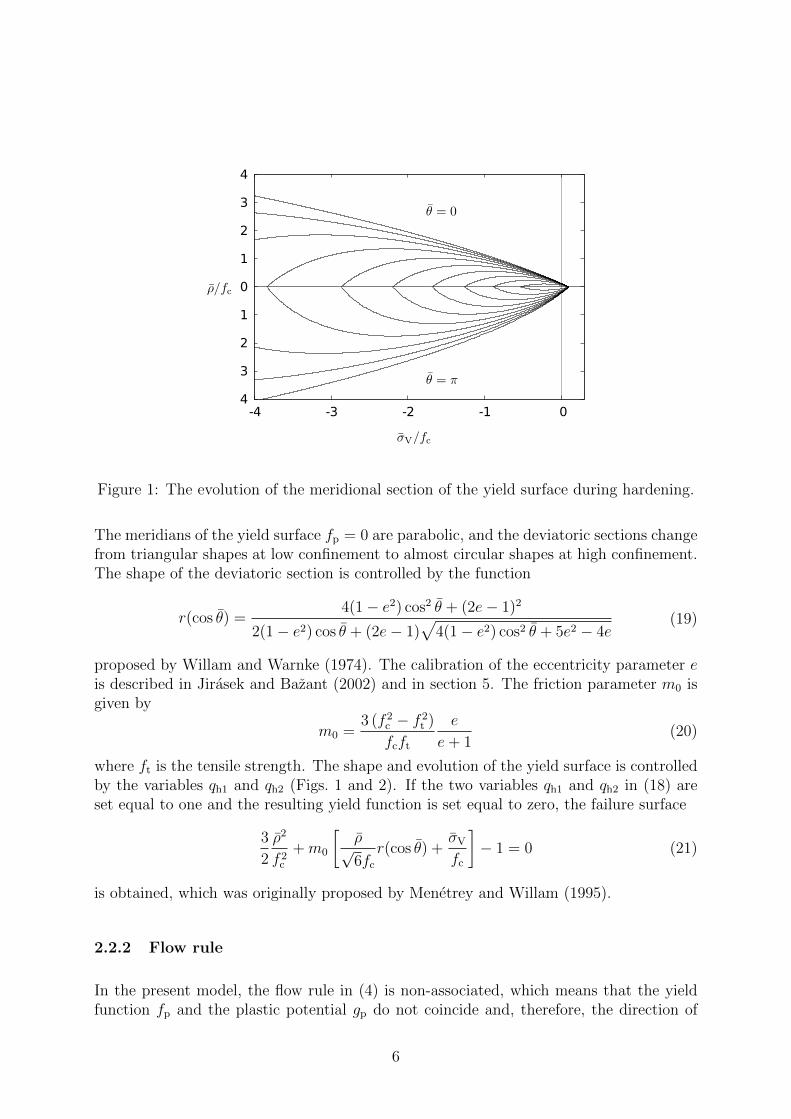
Figure 1: The evolution of the meridional section of the yield surface during hardening.

The meridians of the yield surface fp = 0 are parabolic, and the deviatoric sections changefrom triangular shapes at low confinement to almost circular shapes at high confinement.The shape of the deviatoric section is controlled by the function

r(cos θ) =4(1− e2) cos2 θ + (2e− 1)2

2(1− e2) cos θ + (2e− 1)√

4(1− e2) cos2 θ + 5e2 − 4e(19)

proposed by Willam and Warnke (1974). The calibration of the eccentricity parameter eis described in Jirasek and Bazant (2002) and in section 5. The friction parameter m0 isgiven by

m0 =3 (f 2

c − f 2t )

fcft

e

e+ 1(20)

where ft is the tensile strength. The shape and evolution of the yield surface is controlledby the variables qh1 and qh2 (Figs. 1 and 2). If the two variables qh1 and qh2 in (18) areset equal to one and the resulting yield function is set equal to zero, the failure surface

3

2

ρ2

f 2c

+m0

[ρ√6fc

r(cos θ) +σV

fc

]− 1 = 0 (21)

is obtained, which was originally proposed by Menetrey and Willam (1995).

2.2.2 Flow rule

In the present model, the flow rule in (4) is non-associated, which means that the yieldfunction fp and the plastic potential gp do not coincide and, therefore, the direction of

6

Figure 2: The evolution of the deviatoric section of the yield surface during hardening fora constant volumetric stress of σV = −fc/3.

the plastic flow ∂gp/∂σ is not normal to the yield surface. The plastic potential is givenas

gp(σV, ρ;κp) =

{[1− qh1(κp)]

(ρ√6fc

+σV

fc

)2

+

√3

2

ρ

fc

}2

+ q2h1(κp)

(m0ρ√

6fc

+mg(σV, κp)

fc

) (22)

where

mg(σV, κp) = Ag (κp)Bg (κp) fc expσV − qh2(κp)ft/3

Bg (κp) fc

(23)

is a variable controlling the ratio of volumetric and deviatoric plastic flow. Here, Ag (κp)and Bg (κp), which depend on qh2(κp), are derived from assumptions on the plastic flowin uniaxial tension and compression in the post-peak regime.

The derivation of these two variables is illustrated in the following paragraphs. Here,

the notation m ≡ ∂gp

∂σis introduced. In the principal stress space, the plastic flow

tensor m has three components, m1, m2 and m3 associated with the three principal stresscomponents. The flow rule (4) is split into a volumetric and a deviatoric part, i.e., thegradient of the plastic potential is decomposed as

m =∂g

∂σ=

∂g

∂σV

∂σV

∂σ+∂g

∂ρ

∂ρ

∂σ(24)

Taking into account that ∂σV/∂σ = δ/3 and ∂ρ/∂σ = s/ρ, restricting attention to thepost-peak regime (in which qh1 = 1) and differentiating the plastic potential (22), we

7

rewrite equation (24) as

m =∂g

∂σ=∂mg

∂σV

δ

3fc

+

(3

fc

+m0√

6ρ

)s

fc

(25)

Experimental results for concrete loaded in uniaxial tension indicate that the strainsperpendicular to the loading direction are elastic in the softening regime. Thus, the plasticstrain rate in these directions should be equal to zero (m2 = m3 = 0). Under uniaxialtension, the effective stress state in the post-peak regime is characterised by σ1 = ftqh2,σ2 = σ3 = 0, σV = ftqh2/3, s1 = 2ftqh2/3, s2 = s3 = −ftqh2/3 and ρ =

√2/3ftqh2.

Substituting this into (25) and enforcing the condition m2 = m3 = 0, we obtain anequation from which

∂mg

∂σV

∣∣σV=ftqh2/3 =

3ftqh2

fc

+m0

2(26)

In uniaxial compressive experiments, a volumetric expansion is observed in the softeningregime. Thus, the inelastic lateral strains are positive while the inelastic axial strain isnegative. In the present approach, a constant ratio Df = −m2/m1 = −m3/m1 betweenlateral and axial plastic strain rates in the softening regime is assumed. The effective stressstate at the end of hardening under uniaxial compression is characterised by σ1 = −fcqh2,σ2 = σ3 = 0, σV = −fcqh2/3, s1 = −2fcqh2/3, s2 = s3 = fcqh2/3 and ρ =

√2/3fcqh2.

Substituting this into (25) and enforcing the condition m2 = m3 = −Dfm1, we get anequation from which

∂mg

∂σV

∣∣σV=−fcqh2/3 =

2Df − 1

Df + 1

(3qh2 +

m0

2

)(27)

Substituting the specific expression for ∂mg/∂σV constructed by differentiation of (23)into (26) and (27), we obtain two equations from which parameters

Ag =3ftqh2

fc

+m0

2(28)

Bg =(qh2/3) (1 + ft/fc)

lnAg − ln (2Df − 1)− ln (3qh2 +m0/2) + ln (Df + 1)(29)

can be computed. The gradient of the dilation variable mg in (23) decreases with in-creasing confinement. The limit σV → −∞ corresponds to purely deviatoric flow. As inCDPM1, the plastic potential does not depend on the third Haigh-Westergaard coordinate(Lode angle θ), which increases the efficiency of the implementation and the robustnessof the model.

8

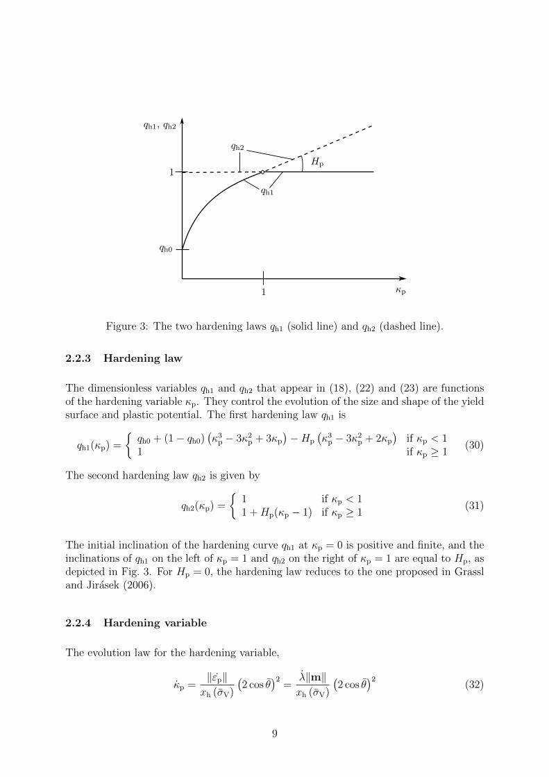
Figure 3: The two hardening laws qh1 (solid line) and qh2 (dashed line).

2.2.3 Hardening law

The dimensionless variables qh1 and qh2 that appear in (18), (22) and (23) are functionsof the hardening variable κp. They control the evolution of the size and shape of the yieldsurface and plastic potential. The first hardening law qh1 is

qh1(κp) =

{qh0 + (1− qh0)

(κ3

p − 3κ2p + 3κp

)−Hp

(κ3

p − 3κ2p + 2κp

)if κp < 1

1 if κp ≥ 1(30)

The second hardening law qh2 is given by

qh2(κp) =

{1 if κp < 11 +Hp(κp − 1) if κp ≥ 1

(31)

The initial inclination of the hardening curve qh1 at κp = 0 is positive and finite, and theinclinations of qh1 on the left of κp = 1 and qh2 on the right of κp = 1 are equal to Hp, asdepicted in Fig. 3. For Hp = 0, the hardening law reduces to the one proposed in Grassland Jirasek (2006).

2.2.4 Hardening variable

The evolution law for the hardening variable,

κp =‖εp‖xh (σV)

(2 cos θ

)2=

λ‖m‖xh (σV)

(2 cos θ

)2(32)

9

sets the rate of the hardening variable equal to the norm of the plastic strain rate scaledby a hardening ductility measure

xh (σV) =

Ah − (Ah −Bh) exp (−Rh(σV)/Ch) if Rh(σV) ≥ 0

Eh exp(Rh(σV)/Fh) +Dh if Rh(σV) < 0(33)

For pure volumetric stress states, θ in (32) is set to zero. The dependence of the scalingfactor xh on the volumetric stress σV is constructed such that the model response is moreductile under compression. The variable

Rh(σV) = − σV

fc

− 1

3(34)

is a linear function of the volumetric effective stress. Model parameters Ah, Bh, Ch andDh are calibrated from the values of strain at peak stress under uniaxial tension, uniaxialcompression and triaxial compression, whereas the parameters Eh and Fh are determinedfrom the conditions of a smooth transition between the two parts of equation (33) atRh = 0:

Eh = Bh −Dh (35)

Fh =(Bh −Dh)Ch

Ah −Bh

(36)

This definition of the hardening variable is identical to the one in CDPM1 described inGrassl and Jirasek (2006), where the calibration procedure for this part of the model isdescribed.

2.3 Damage part

Damage is initiated when the maximum equivalent strain in the history of the materialreaches the threshold ε0 = ft/E. For uniaxial tension only, the equivalent strain couldbe chosen as ε = σt/E, where σt is the effective uniaxial tensile stress. Thus, damageinitiation would be linked to the axial elastic strain. However, for general triaxial stressstates a more advanced equivalent strain expression is required, which predicts damageinitiation when the strength envelope is reached. This expression is determined from theyield surface (fp = 0) by setting qh1 = 1 and qh2 = ε/ε0. From this quadratic equationfor ε, the equivalent strain is determined as

ε =ε0m0

2

(ρ√6fc

r (cos θ) +σV

fc

)+

√ε2

0m20

4

(ρ√6fc

r (cos θ) +σV

fc

)2

+3ε2

0ρ2

2f 2c

(37)

For uniaxial tension, the effective stress state is defined as σ1 = σt, σ2 = σ3 = 0, σV =σt/3, s1 = 2σt/3, s2 = s3 = −σt/3, ρ =

√2/3σt and r(cos θ) = 1/e. Setting this into (37)

10

and using the definition of m0 in (20) gives

ε = ε0σt

ft

= σt/E (38)

which is suitable equivalent strain for modelling tensile failure. For uniaxial compression,the effective stress state is defined as σ1 = −σc, σ2 = σ3 = 0, σV = −σc/3, s1 = −2/3σc,s2 = s3 = 1/3σc, ρ =

√2/3σc, and r(cos θ) = 1. Here, σc is the magnitude of the effective

compressive stress. Setting this into (37), the equivalent strain is

ε =σcε0

fc

=σcft

Efc

(39)

If σc = (fc/ft)σt, the equivalent strain is again equal to the axial elastic strain componentin uniaxial tension. Consequently, the equivalent strain definition in (37) is suitable forboth tension and compression, which is very convenient for relating the damage variablesin tension and compression to stress-inelastic strain curves.

The damage variables ωt and ωc in (1) are determined so that a prescribed stress-inelasticstrain relation in uniaxial tension is obtained. Since, the damage variables are evaluatedfor general triaxial stress states, the inelastic strain in uniaxial tension has to be expressedby suitable scalar history variables, which are obtained from total and plastic straincomponents. To illustrate the choice of these components, a 1D damage-plastic stress-strain law of the form

σ = (1− ω) σ = (1− ω)E (ε− εp) (40)

is considered. Here, ω is the damage variable. This law can also be written as

σ = E {ε− [εp + ω (ε− εp)]} = E (ε− εi) (41)

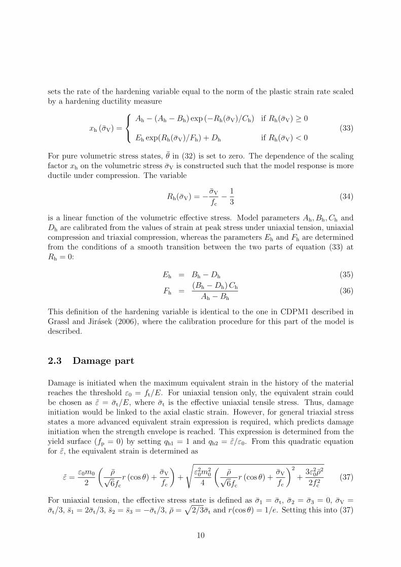
where εi is the inelastic strain which is subtracted from the total strain. The geometricalinterpretation of the inelastic strain and its split for monotonic uniaxial tension, linearhardening plasticity and linear damage evolution are shown in Fig. 4. Furthermore, theway how the hardening influences damage and plasticity dissipation has been discussedin Grassl (2009). The part ω (ε− εp) is reversible and εp is irreversible. The damagevariable is chosen, so that a softening law is obtained, which relates the stress to theinelastic strain, which is written here in generic form as

σ = fs (εi) (42)

Setting (41) equal with (42) allows for determining the damage variable ω.

However, the inelastic strain εi in (41) and (42) needs to be expressed by history variables,so that the expression for the damage variable can be used for non-monotonic loading.Furthermore, to be able to describe also the influence of multiaxial stress states on thedamage evolution, the inelastic strain in (42) is replaced by different history variables thanthe inelastic strain in (41). The choice of the history variables for tension and compression

11

Figure 4: Geometrical meaning of the inelastic strain εi for the combined damage-plasticity model. The inelastic strain is composed of reversible ω (ε− εp) and irreversibleεp parts. The dashed lines represent elastic unloading with the same stiffness as the initialelastic loading.

12

is explained in sections. 2.3.1 and 2.3.2.

2.3.1 History variables for tension

The tensile damage variable ωt in (1) is defined by three history variables κdt, κdt1 andκdt2. The variable κdt is used in the definition of the inelastic strain in (41), while κdt1

and κdt2 enter the definition of the inelastic strain in (42). The history variable κdt isdetermined from εt using (6) and (7). Here, εt is given implicitly in incremental form by

˙εt = ˙ε (43)

with ε given in (37). For κdt1, the inelastic strain component related the plastic strain εp

is replaced by

κdt1 =

1

xs

‖εp‖ if κdt > 0 and κdt > ε0

0 if κdt = 0 or κdt < ε0

(44)

Here, the pre-peak plastic strains do not contribute to this history variable, since κdt1 isonly nonzero, if κdt > ε0. Finally, the third history variable is related to κdt as

κdt2 =κdt

xs

(45)

In (44) and (45), xs is a ductility measure, which describes the influence of multiaxialstress states on the softening response, see Sec. 2.3.4.

2.3.2 History variables for compression

The compression damage variable ωc is also defined by three history variables κdc, κdc1

and κdc2. Analogous to the tensile case, the variable κdc is used in the definition of theinelastic strain in (41), while κdc1 and κdc2 enter the definition of the equivalent strain in(42). In addition, a variable αc is introduced which distinguishes tensile and compressivestresses. It has the form

αc =3∑i=1

σpci (σpti + σpci)

‖σp‖2(46)

where σpti and σpci are the components of the compressive and tensile part of the principaleffective stresses, respectively, which were previously used for the general stress strain lawin (1). The variable αc varies from 0 for pure tension to 1 for pure compression. Forinstance, for the mixed tensile compressive effective stress state σp = {−σ, 0.2σ, 0.1σ},considered in Sec. 2.1, the variable is αc = 0.95.

The history variable κdc is determined from εc using (9) and (10), where, analogous to

13

the tensile case, the εc is specified implicitly by

˙εc = αc˙ε (47)

The other two history variables are

κdc1 =

αcβc

xs

‖εp‖ if κdt > 0 ∧ κdt > ε0

0 if κdt = 0 ∨ κdt < ε0

(48)

and

κdc2 =κdc

xs

(49)

In (48), the factor βc is

βc =ftqh2

√2/3

ρ√

1 + 2D2f

(50)

This factor provides a smooth transition from pure damage to damage-plasticity softeningprocesses, which can occur during cyclic loading, as described in section 2.3.5.

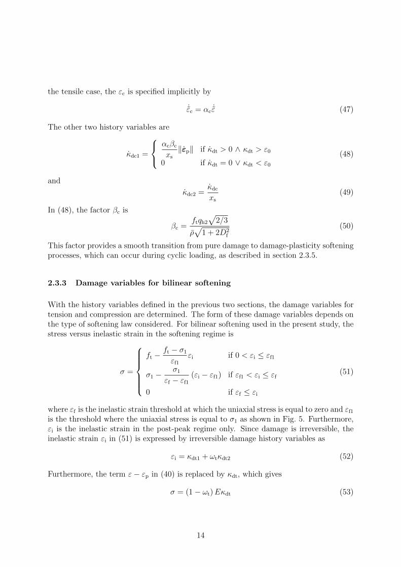
2.3.3 Damage variables for bilinear softening

With the history variables defined in the previous two sections, the damage variables fortension and compression are determined. The form of these damage variables depends onthe type of softening law considered. For bilinear softening used in the present study, thestress versus inelastic strain in the softening regime is

σ =

ft −

ft − σ1

εf1

εi if 0 < εi ≤ εf1

σ1 −σ1

εf − εf1

(εi − εf1) if εf1 < εi ≤ εf

0 if εf ≤ εi

(51)

where εf is the inelastic strain threshold at which the uniaxial stress is equal to zero and εf1

is the threshold where the uniaxial stress is equal to σ1 as shown in Fig. 5. Furthermore,εi is the inelastic strain in the post-peak regime only. Since damage is irreversible, theinelastic strain εi in (51) is expressed by irreversible damage history variables as

εi = κdt1 + ωtκdt2 (52)

Furthermore, the term ε− εp in (40) is replaced by κdt, which gives

σ = (1− ωt)Eκdt (53)

14

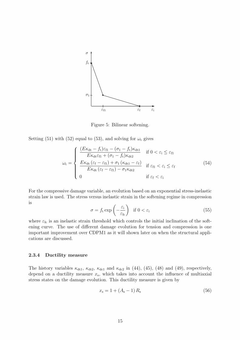
Figure 5: Bilinear softening.

Setting (51) with (52) equal to (53), and solving for ωt gives

ωt =

(Eκdt − ft)εf1 − (σ1 − ft)κdt1

Eκdtεf1 + (σ1 − ft)κdt2

if 0 < εi ≤ εf1

Eκdt (εf − εf1) + σ1 (κdt1 − εf)

Eκdt (εf − εf1)− σ1κdt2

if εf1 < εi ≤ εf

0 if εf < εi

(54)

For the compressive damage variable, an evolution based on an exponential stress-inelasticstrain law is used. The stress versus inelastic strain in the softening regime in compressionis

σ = ft exp

(− εi

εfc

)if 0 < εi (55)

where εfc is an inelastic strain threshold which controls the initial inclination of the soft-ening curve. The use of different damage evolution for tension and compression is oneimportant improvement over CDPM1 as it will shown later on when the structural appli-cations are discussed.

2.3.4 Ductility measure

The history variables κdt1, κdt2, κdc1 and κdc2 in (44), (45), (48) and (49), respectively,depend on a ductility measure xs, which takes into account the influence of multiaxialstress states on the damage evolution. This ductility measure is given by

xs = 1 + (As − 1)Rs (56)

15

where Rs is

Rs =

−√

6σV

ρif σV ≤ 0

0 if σV > 0(57)

and As is a model parameter. For uniaxial compression σV/ρ = −1/√

6, so that Rs = 1and xs = As, which simplifies the calibration of the softening response in this case.

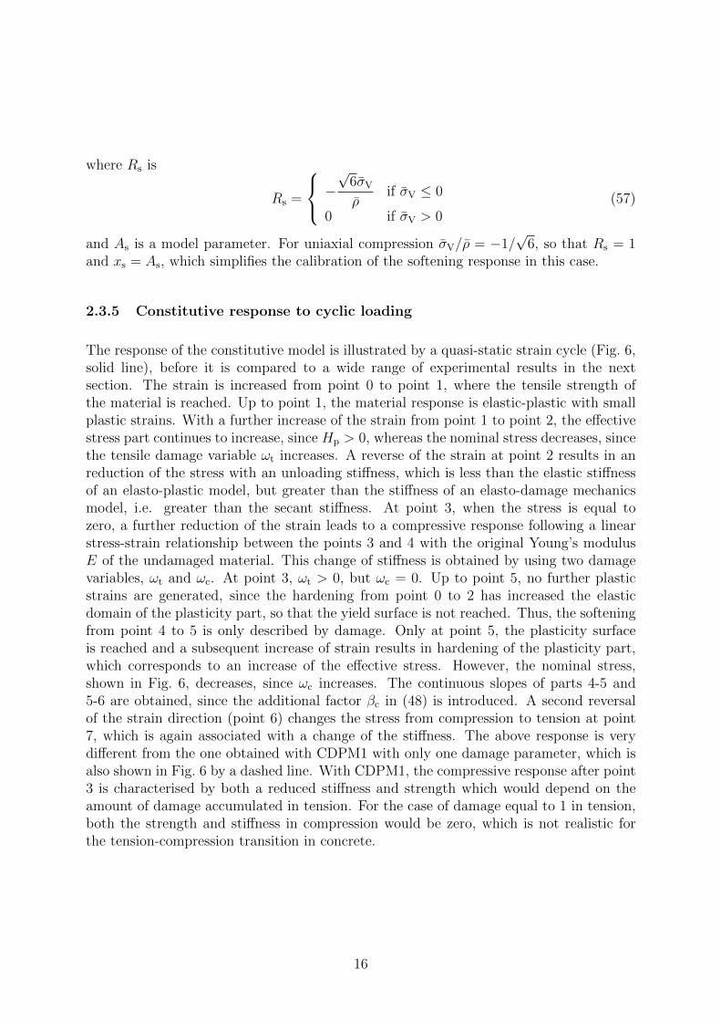
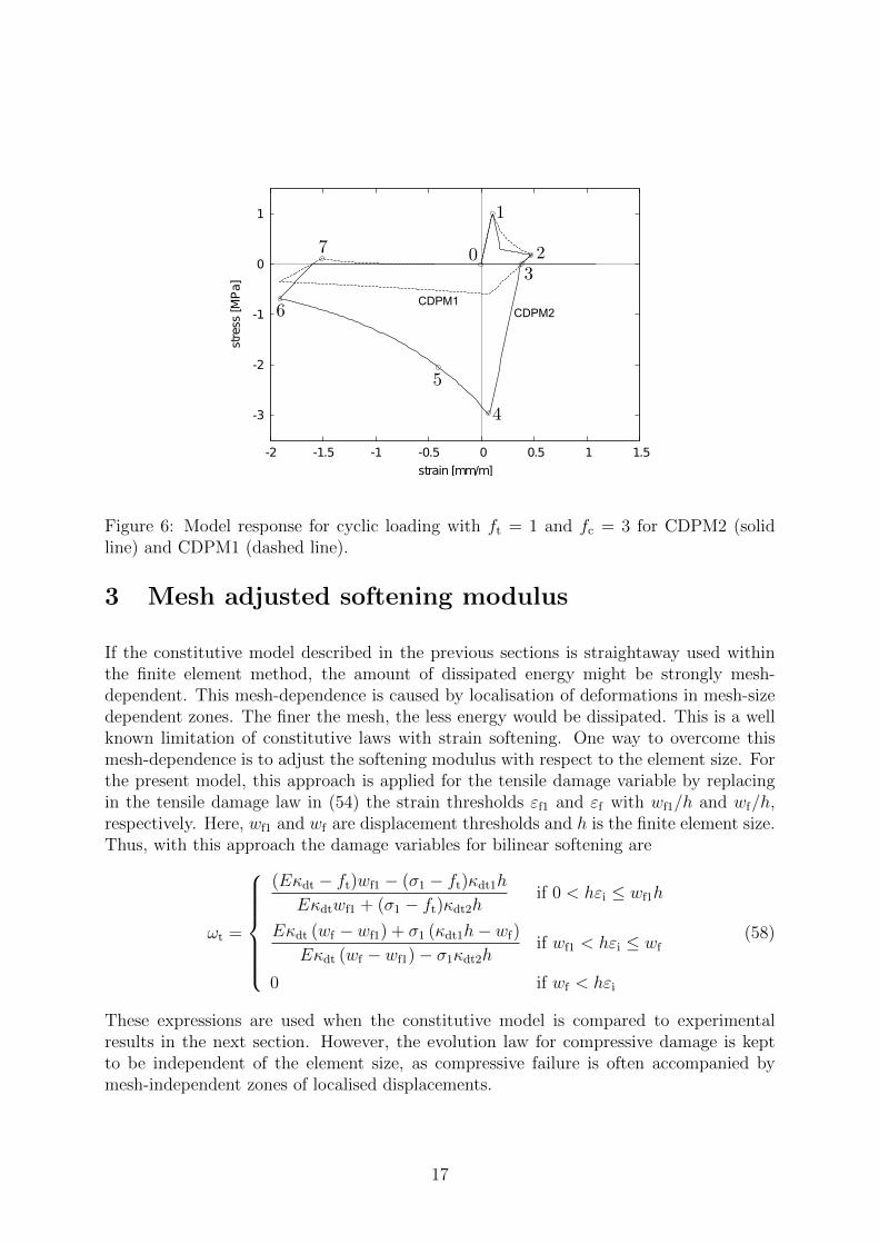
2.3.5 Constitutive response to cyclic loading

The response of the constitutive model is illustrated by a quasi-static strain cycle (Fig. 6,solid line), before it is compared to a wide range of experimental results in the nextsection. The strain is increased from point 0 to point 1, where the tensile strength ofthe material is reached. Up to point 1, the material response is elastic-plastic with smallplastic strains. With a further increase of the strain from point 1 to point 2, the effectivestress part continues to increase, since Hp > 0, whereas the nominal stress decreases, sincethe tensile damage variable ωt increases. A reverse of the strain at point 2 results in anreduction of the stress with an unloading stiffness, which is less than the elastic stiffnessof an elasto-plastic model, but greater than the stiffness of an elasto-damage mechanicsmodel, i.e. greater than the secant stiffness. At point 3, when the stress is equal tozero, a further reduction of the strain leads to a compressive response following a linearstress-strain relationship between the points 3 and 4 with the original Young’s modulusE of the undamaged material. This change of stiffness is obtained by using two damagevariables, ωt and ωc. At point 3, ωt > 0, but ωc = 0. Up to point 5, no further plasticstrains are generated, since the hardening from point 0 to 2 has increased the elasticdomain of the plasticity part, so that the yield surface is not reached. Thus, the softeningfrom point 4 to 5 is only described by damage. Only at point 5, the plasticity surfaceis reached and a subsequent increase of strain results in hardening of the plasticity part,which corresponds to an increase of the effective stress. However, the nominal stress,shown in Fig. 6, decreases, since ωc increases. The continuous slopes of parts 4-5 and5-6 are obtained, since the additional factor βc in (48) is introduced. A second reversalof the strain direction (point 6) changes the stress from compression to tension at point7, which is again associated with a change of the stiffness. The above response is verydifferent from the one obtained with CDPM1 with only one damage parameter, which isalso shown in Fig. 6 by a dashed line. With CDPM1, the compressive response after point3 is characterised by both a reduced stiffness and strength which would depend on theamount of damage accumulated in tension. For the case of damage equal to 1 in tension,both the strength and stiffness in compression would be zero, which is not realistic forthe tension-compression transition in concrete.

16

-3

-2

-1

0

1

-2 -1.5 -1 -0.5 0 0.5 1 1.5

stress

[MPa]

strain [mm/m]

CDPM1CDPM2

Figure 6: Model response for cyclic loading with ft = 1 and fc = 3 for CDPM2 (solidline) and CDPM1 (dashed line).

3 Mesh adjusted softening modulus

If the constitutive model described in the previous sections is straightaway used withinthe finite element method, the amount of dissipated energy might be strongly mesh-dependent. This mesh-dependence is caused by localisation of deformations in mesh-sizedependent zones. The finer the mesh, the less energy would be dissipated. This is a wellknown limitation of constitutive laws with strain softening. One way to overcome thismesh-dependence is to adjust the softening modulus with respect to the element size. Forthe present model, this approach is applied for the tensile damage variable by replacingin the tensile damage law in (54) the strain thresholds εf1 and εf with wf1/h and wf/h,respectively. Here, wf1 and wf are displacement thresholds and h is the finite element size.Thus, with this approach the damage variables for bilinear softening are

ωt =

(Eκdt − ft)wf1 − (σ1 − ft)κdt1h

Eκdtwf1 + (σ1 − ft)κdt2hif 0 < hεi ≤ wf1h

Eκdt (wf − wf1) + σ1 (κdt1h− wf)

Eκdt (wf − wf1)− σ1κdt2hif wf1 < hεi ≤ wf

0 if wf < hεi

(58)

These expressions are used when the constitutive model is compared to experimentalresults in the next section. However, the evolution law for compressive damage is keptto be independent of the element size, as compressive failure is often accompanied bymesh-independent zones of localised displacements.

17

4 Implementation

The present constitutive model has been implemented within the framework of the nonlin-ear finite element method, where the continuous loading process is replaced by incrementaltime steps. In each step the boundary value problem (global level) and the integration ofthe constitutive laws (local level) are solved.

For the boundary value problem on the global level, the usual incremental-iterative solu-tion strategy is used, in the form of a modified Newton-Raphson iteration method. Forthe local problem, the updated values (·)(n+1) of the stress and the internal variables atthe end of the step are obtained by a fully implicit (backward Euler) integration of the

rate form of the constitutive equations, starting from their known values (·)(n) at thebeginning of the step and applying the given strain increment ∆ε = ε(n+1) − ε(n). Theintegration scheme is divided into two sequential steps, corresponding to the plastic anddamage parts of the model. In the plastic part, the plastic strain εp and the effectivestress σ at the end of the step are determined. In the damage part, the damage variablesωt and ωc, and the nominal stress σ at the end of the step are obtained. The implemen-tation strategy for the local problem, described in detail in Grassl and Jirasek (2006) forCDPM1, applies to the present model as well. To improve the robustness of the model, asubincrementation scheme is employed for the integration of the plasticity part.

5 Comparison with experimental results

In this section, the model response is compared to five groups of experiments reported inthe literature. For each group of experiments, the physical constants Young’s modulus E,Poisson’s ratio ν, tensile strength ft, compressive strength fc and tensile fracture energyGFt are adjusted to obtain a fit for the different types of concrete used in the experiments.The first four constants are model parameters. The last physical constant, GFt, is directlyrelated to model parameters. For the bilinear softening law in section 2.3.3, the tensilefracture energy is

GFt = ftwf1/2 + σ1wf/2 (59)

For σ1/ft = 0.3 and wf1/wf = 0.15 (shown by Jirasek and Zimmermann (1998) to resultin a good fit for concrete failure), the expression for the fracture energy reduces to GFt =ftwf/4.444. The compressive energy is GFc = fcεfclcAs, where lc is the length in whichthe compressive displacement are assumed to localise and As is the ductility measure inSec. 2.3.4. If no experimental results are available, the five constants can be determinedusing, for instance, the CEB-FIP Model Code (CEB, 1991).

The other model parameters are set to their default values for all groups. The eccentricityconstant e that controls the shape of the deviatoric section is evaluated using the formula

18

in Jirasek and Bazant (2002), p. 365:

e =1 + ε

2− ε, where ε =

ft

fbc

f 2bc − f 2

c

f 2c − f 2

t

(60)

where fbc is the strength in equibiaxial compression, which is estimated as fbc = 1.16fc

according to the experimental results reported in Kupfer et al. (1969). Parameter qh0 isthe dimensionless ratio qh0 = fc0/fc, where fc0 is the compressive stress at which the initialyield limit is reached in the plasticity model for uniaxial compression. Its default valueis qh0 = 0.3. For the hardening modulus the default value is Hp = 0.01. Furthermore,the default value of the parameter of the flow rule is chosen as Df = 0.85, which yieldsa good agreement with experimental results in uniaxial compression. The determinationof parameters Ah, Bh, Ch and Dh that influence the hardening ductility measure is moredifficult. The effective stress varies within the hardening regime, even for monotonicloading, so that the ratio of axial and lateral plastic strain rate is not constant. Thus, anexact relation of all four model parameters to measurable material properties cannot beconstructed. In Grassl and Jirasek (2006), it has been shown that a reasonable responseis obtained with parameters Ah = 0.08, Bh = 0.003, Ch = 2 and Dh = 1 × 10−6. Thesevalues were also used in the present study. Furthermore, the element size h in the damagelaws in Section 3 was chosen as h = 0.1 m.

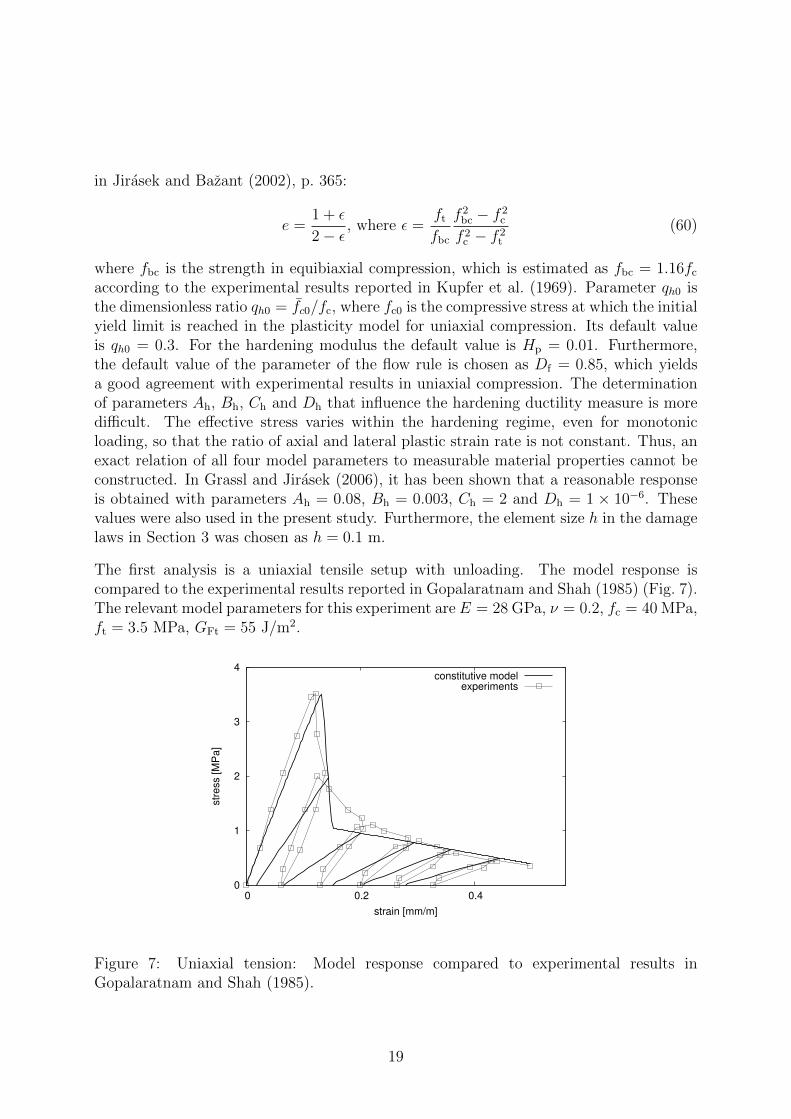
The first analysis is a uniaxial tensile setup with unloading. The model response iscompared to the experimental results reported in Gopalaratnam and Shah (1985) (Fig. 7).The relevant model parameters for this experiment are E = 28 GPa, ν = 0.2, fc = 40 MPa,ft = 3.5 MPa, GFt = 55 J/m2.

0

1

2

3

4

0 0.2 0.4

str

ess [M

Pa]

strain [mm/m]

constitutive modelexperiments

Figure 7: Uniaxial tension: Model response compared to experimental results inGopalaratnam and Shah (1985).

19

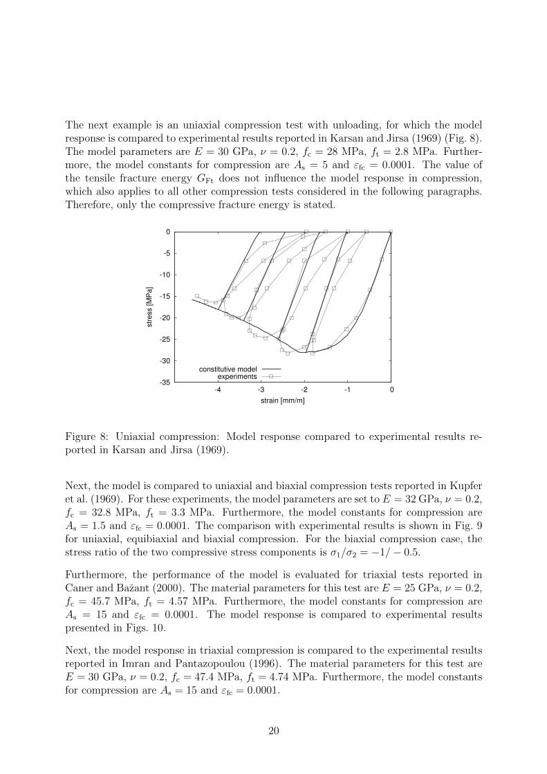
The next example is an uniaxial compression test with unloading, for which the modelresponse is compared to experimental results reported in Karsan and Jirsa (1969) (Fig. 8).The model parameters are E = 30 GPa, ν = 0.2, fc = 28 MPa, ft = 2.8 MPa. Further-more, the model constants for compression are As = 5 and εfc = 0.0001. The value ofthe tensile fracture energy GFt does not influence the model response in compression,which also applies to all other compression tests considered in the following paragraphs.Therefore, only the compressive fracture energy is stated.

-35

-30

-25

-20

-15

-10

-5

0

-4 -3 -2 -1 0

str

ess [M

Pa]

strain [mm/m]

constitutive modelexperiments

Figure 8: Uniaxial compression: Model response compared to experimental results re-ported in Karsan and Jirsa (1969).

Next, the model is compared to uniaxial and biaxial compression tests reported in Kupferet al. (1969). For these experiments, the model parameters are set to E = 32 GPa, ν = 0.2,fc = 32.8 MPa, ft = 3.3 MPa. Furthermore, the model constants for compression areAs = 1.5 and εfc = 0.0001. The comparison with experimental results is shown in Fig. 9for uniaxial, equibiaxial and biaxial compression. For the biaxial compression case, thestress ratio of the two compressive stress components is σ1/σ2 = −1/− 0.5.

Furthermore, the performance of the model is evaluated for triaxial tests reported inCaner and Bazant (2000). The material parameters for this test are E = 25 GPa, ν = 0.2,fc = 45.7 MPa, ft = 4.57 MPa. Furthermore, the model constants for compression areAs = 15 and εfc = 0.0001. The model response is compared to experimental resultspresented in Figs. 10.

Next, the model response in triaxial compression is compared to the experimental resultsreported in Imran and Pantazopoulou (1996). The material parameters for this test areE = 30 GPa, ν = 0.2, fc = 47.4 MPa, ft = 4.74 MPa. Furthermore, the model constantsfor compression are As = 15 and εfc = 0.0001.

20

-40

-30

-20

-10

0

-4 -2 0 2 4 6

str

ess [

MP

a]

strain [mm/m]

const. -1/0const. -1/-0.5

const. -1/-1exp. -1/0

exp. -1/-0.5exp. -1/-1

Figure 9: Uniaxial and biaxial compression: Model response compared to experimentalresults reported in Kupfer et al. (1969).

-1000

-800

-600

-400

-200

0

-50 -40 -30 -20 -10 0

stress

[MPa]

strain [mm/m]

constitutivemodelexperiments

20

100

200

400

Figure 10: Confined compression: Model response compared to experiments used in Canerand Bazant (2000).

Finally, the model response in hydrostatic compression is compared to the experimentalresults reported in Caner and Bazant (2000). The material parameters are the same asfor the triaxial test shown in Fig. 10.

Overall, the agreement of the model response with the experimental results is very good.The model is able to represent the strength of concrete in tension and multiaxial compres-sion. In addition, the strains at maximum stress in tension and compression agree well

21

-200

-150

-100

-50

0

-60 -40 -20 0 20 40

stress

[MPa]

strain [mm/m]

const. responseexperiments

Figure 11: Confined compression: Model response compared to experiments reported inImran and Pantazopoulou (1996).

-600

-500

-400

-300

-200

-100

0

-70 -60 -50 -40 -30 -20 -10 0

str

ess [M

Pa]

strain [mm/m]

constitutive modelexperiments

Figure 12: Hydrostatic compression: Model response compared to experiments reportedin Caner and Bazant (2000).

with the experimental results. The bilinear stress-crack opening curve that was used re-sults in a good approximation of the softening curve in uniaxial tension and compression.With the above comparisons, it is demonstrated that CDPM2, provides, very similar toCDPM1, a very good agreement with experimental results.

22

6 Structural analysis

The performance of the proposed constitutive model is further evaluated by structuralanalysis of three fracture tests. The main objective of this part of the study is to demon-strate that the structural response obtained with the model is mesh-independent. This isachieved by adjusting the softening modulus with respect to the element size (section 3).

6.1 Three point bending test

The first structural example is a three-point bending test of a single-edge notched beamreported by Kormeling and Reinhardt (1982). The experiment is modelled by triangularplane strain finite elements with three mesh sizes. The geometry and loading set up isshown in Fig. 13. The input parameters are chosen as E = 20 GPa, ν = 0.2, ft = 2.4 MPa,Gft = 100 N/m, fc = 24 MPa (Grassl and Jirasek, 2006a). All other parameters are setto their default values described in section 5. For this type of analysis, local stress-strainrelations with strain softening are known to result in mesh-dependent load-displacementcurves. The capability of the adjustment of the softening modulus approach presented insection 3 to overcome this mesh-dependence is assessed with this test. The global response

Figure 13: Three point bending test: Geometry and loading setup. The out-of-planethickness is 0.1 m. The notch thickness is 5 mm.

in the form of load-Crack Mouth Opening Displacement (CMOD) is shown in Fig. 14.The local response in the form of tensile damage patterns at loading stages marked inFig. 14 for the three meshes is shown in Fig. 15.

Overall, the load-CMOD curves in Fig. 14 are in good agreement with the experimentalresults and almost mesh independent. On the other hand, the damage zones in Fig. 15depend on the mesh size.

23

0

0.2

0.4

0.6

0.8

1

1.2

1.4

1.6

0 0.2 0.4 0.6 0.8 1

load [kN

]

displacement [mm]

coarse meshmedium mesh

fine meshexperimental bounds

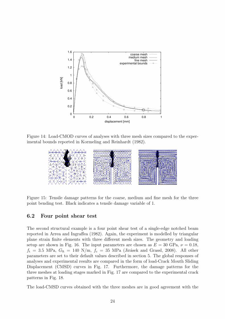
Figure 14: Load-CMOD curves of analyses with three mesh sizes compared to the exper-imental bounds reported in Kormeling and Reinhardt (1982).

Figure 15: Tensile damage patterns for the coarse, medium and fine mesh for the threepoint bending test. Black indicates a tensile damage variable of 1.

6.2 Four point shear test

The second structural example is a four point shear test of a single-edge notched beamreported in Arrea and Ingraffea (1982). Again, the experiment is modelled by triangularplane strain finite elements with three different mesh sizes. The geometry and loadingsetup are shown in Fig. 16. The input parameters are chosen as E = 30 GPa, ν = 0.18,ft = 3.5 MPa, Gft = 140 N/m, fc = 35 MPa (Jirasek and Grassl, 2008). All otherparameters are set to their default values described in section 5. The global responses ofanalyses and experimental results are compared in the form of load-Crack Mouth SlidingDisplacement (CMSD) curves in Fig. 17. Furthermore, the damage patterns for thethree meshes at loading stages marked in Fig. 17 are compared to the experimental crackpatterns in Fig. 18.

The load-CMSD curves obtained with the three meshes are in good agreement with the

24

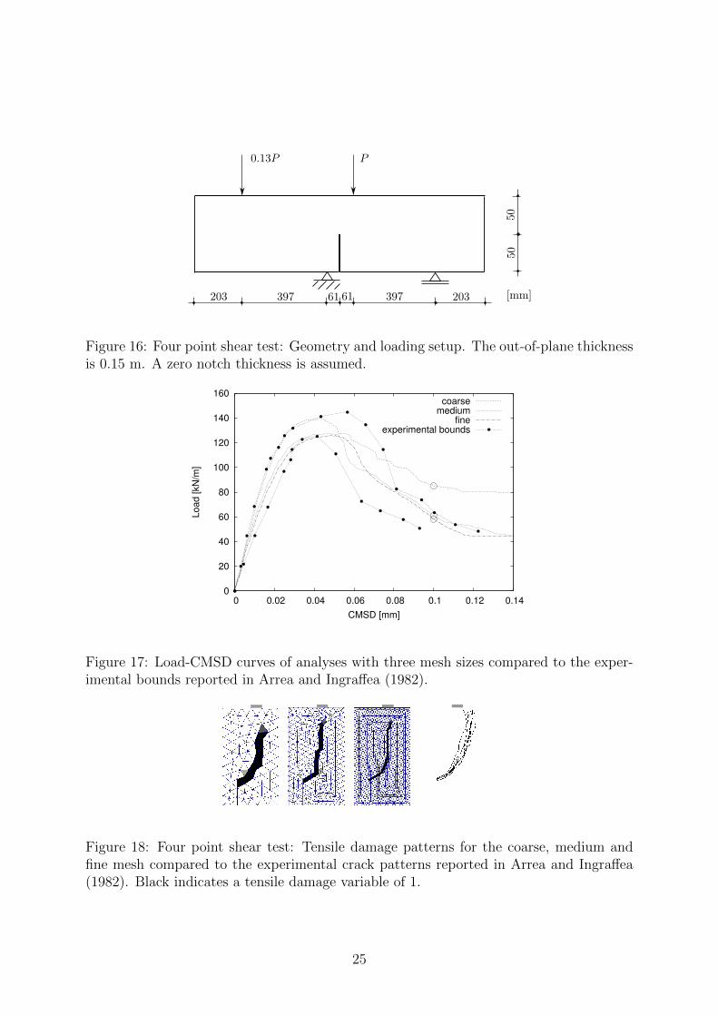
Figure 16: Four point shear test: Geometry and loading setup. The out-of-plane thicknessis 0.15 m. A zero notch thickness is assumed.

0

20

40

60

80

100

120

140

160

0 0.02 0.04 0.06 0.08 0.1 0.12 0.14

Loa

d [kN

/m]

CMSD [mm]

coarsemedium

fineexperimental bounds

Figure 17: Load-CMSD curves of analyses with three mesh sizes compared to the exper-imental bounds reported in Arrea and Ingraffea (1982).

Figure 18: Four point shear test: Tensile damage patterns for the coarse, medium andfine mesh compared to the experimental crack patterns reported in Arrea and Ingraffea(1982). Black indicates a tensile damage variable of 1.

25

50

0

50

P

150

36.8

50

200

[mm]

ε

(a) (b)

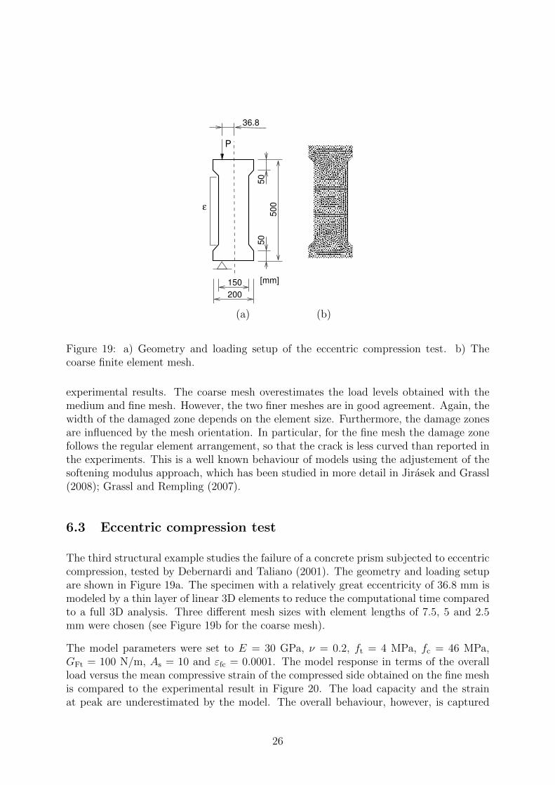
Figure 19: a) Geometry and loading setup of the eccentric compression test. b) Thecoarse finite element mesh.

experimental results. The coarse mesh overestimates the load levels obtained with themedium and fine mesh. However, the two finer meshes are in good agreement. Again, thewidth of the damaged zone depends on the element size. Furthermore, the damage zonesare influenced by the mesh orientation. In particular, for the fine mesh the damage zonefollows the regular element arrangement, so that the crack is less curved than reported inthe experiments. This is a well known behaviour of models using the adjustement of thesoftening modulus approach, which has been studied in more detail in Jirasek and Grassl(2008); Grassl and Rempling (2007).

6.3 Eccentric compression test

The third structural example studies the failure of a concrete prism subjected to eccentriccompression, tested by Debernardi and Taliano (2001). The geometry and loading setupare shown in Figure 19a. The specimen with a relatively great eccentricity of 36.8 mm ismodeled by a thin layer of linear 3D elements to reduce the computational time comparedto a full 3D analysis. Three different mesh sizes with element lengths of 7.5, 5 and 2.5mm were chosen (see Figure 19b for the coarse mesh).

The model parameters were set to E = 30 GPa, ν = 0.2, ft = 4 MPa, fc = 46 MPa,GFt = 100 N/m, As = 10 and εfc = 0.0001. The model response in terms of the overallload versus the mean compressive strain of the compressed side obtained on the fine meshis compared to the experimental result in Figure 20. The load capacity and the strainat peak are underestimated by the model. The overall behaviour, however, is captured

26

0

50

100

150

200

250

300

350

400

-8 -7 -6 -5 -4 -3 -2 -1 0

load [kN

]

average strain [mm/m]

coarse meshmedium mesh

fine meshexperiment

Figure 20: Comparison of the analysis of the eccentric compression test with the experi-ment.

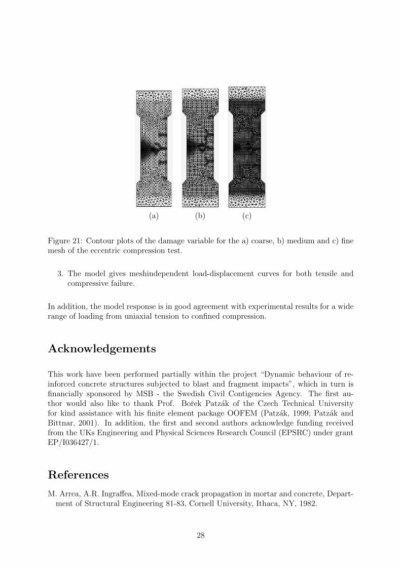
well. The comparison of the load-compressive strain relations for the analyses on meshesof different sizes indicates that the description of this type of compressive failure is nearlymesh-independent. The evolution of the damage zone for the analysis on the coarse meshis depicted in Figure 21 for the final stage of the analyses in Figure 20. On the tensileside several zones of localized damage form, whereas the failure on the compressive sideis described by a diffuse damage zone.

7 Conclusions

The present damage plasticity model CDPM2, which combines a stress-based plasticitypart with a strain based damage mechanics model, is based on an enhancement of analready exisiting damage-plasticity model called CDPM1 (Grassl and Jirasek (2006)).Based on the work presented in this manuscript, the following conclusions can be drawnon the improvements that this constitutive model provides:

1. The model is able to describe realistically the transition from tensile to compressivefailure. This is achieved by the introduction of two separate isotropic damage vari-ables for tension and compression.

2. The model is able to reproduce stress inelastic strain relations with varying ratiosof reversible and irreversible strain components. The ratio can be controlled by thehardening modulus of the plasticity part.

27

(a) (b) (c)

Figure 21: Contour plots of the damage variable for the a) coarse, b) medium and c) finemesh of the eccentric compression test.

3. The model gives meshindependent load-displacement curves for both tensile andcompressive failure.

In addition, the model response is in good agreement with experimental results for a widerange of loading from uniaxial tension to confined compression.

Acknowledgements

This work have been performed partially within the project “Dynamic behaviour of re-inforced concrete structures subjected to blast and fragment impacts”, which in turn isfinancially sponsored by MSB - the Swedish Civil Contigencies Agency. The first au-thor would also like to thank Prof. Borek Patzak of the Czech Technical Universityfor kind assistance with his finite element package OOFEM (Patzak, 1999; Patzak andBittnar, 2001). In addition, the first and second authors acknowledge funding receivedfrom the UKs Engineering and Physical Sciences Research Council (EPSRC) under grantEP/I036427/1.

References

M. Arrea, A.R. Ingraffea, Mixed-mode crack propagation in mortar and concrete, Depart-ment of Structural Engineering 81-83, Cornell University, Ithaca, NY, 1982.

28

F.C. Caner, Z.P. Bazant, Microplane model M4 for concrete: II. Algorithm and calibra-tion, Journal of Engineering Mechanics, ASCE 126 (2000) 954–961.

I. Carol, E. Rizzi, K.J. Willam, On the formulation of anisotropic elastic degradation.I. Theory based on a pseudo-logarithmic damage tensor rate, International Journal ofSolids and Structures 38 (2001) 491–518.

CEB, CEB-FIP Model Code 1990, Design Code, Thomas Telford, London, 1991.

P.G. Debernardi, M. Taliano, Softening behaviour of concrete prisms under eccentriccompressive forces, Magazine of Concrete Research 53 (2001) 239–249.

G. Etse, K.J. Willam, A fracture-energy based constitutive formulation for inelastic behav-ior of plain concrete, Journal of Engineering Mechanics, ASCE 120 (1994) 1983–2011.

S. Fichant, C.L. Borderie, G. Pijaudier-Cabot, Isotropic and anisotropic descriptions ofdamage in concrete structures, Mechanics of Cohesive-Frictional Materials 4 (1999)339–359.

P. Folino, G. Etse, Performance dependent model for normal and high strength concretes,International Journal of Solids and Structures 49 (2012) 701–719.

V.S. Gopalaratnam, S.P. Shah, Softening response of plain concrete in direct tension, ACIJournal Proceedings 82 (1985).

P. Grassl, On a damage-plasticity approach to model concrete failure, Proceedings of theICE - Engineering and Computational Mechanics 162 (2009) 221–231.

P. Grassl, M. Jirasek, Damage-plastic model for concrete failure, International Journal ofSolids and Structures 43 (2006) 7166–7196.

P. Grassl, M. Jirasek, A plastic model with nonlocal damage applied to concrete, Inter-national Journal for Numerical and Analytical Methods in Geomechanics 30 (2006a)71–90.

P. Grassl, K. Lundgren, K. Gylltoft, Concrete in compression: a plasticity theory witha novel hardening law, International Journal of Solids and Structures 39 (2002) 5205–5223.

P. Grassl, R. Rempling, Influence of volumetric-deviatoric coupling on crack predictionin concrete fracture tests, Engineering Fracture Mechanics 74 (2007) 1683–1693.

I. Imran, S.J. Pantazopoulou, Experimental study of plain concrete under triaxial stress,ACI Materials Journal 93 (1996) 589–601.

L. Jason, A. Huerta, G. Pijaudier-Cabot, S. Ghavamian, An elastic plastic damage formu-lation for concrete: Application to elementary tests and comparison with an isotropicdamage model, Computer Methods in Applied Mechanics and Engineering 195 (2006)7077–7092.

29

M. Jirasek, Z.P. Bazant, Inelastic Analysis of Structures, John Wiley and Sons, Chichester,2002.

M. Jirasek, P. Grassl, Evaluation of directional mesh bias in concrete fracture simulationsusing continuum damage models, Engineering Fracture Mechanics 75 (2008) 1921–1943.

M. Jirasek, T. Zimmermann, Rotating crack model with transition to scalar damage,Journal of Engineering Mechanics 124 (1998) 277–284.

J.W. Ju, On energy-based coupled elastoplastic damage theories: Constitutive modelingand computational aspects, International Journal of Solids and Structures 25 (1989)803–833.

M. Kachanov, Continuum model of medium with cracks, Journal of the EngineeringMechanics Division 106 (1980) 1039–1051.

I.D. Karsan, J.O. Jirsa, Behavior of concrete under compressive loadings, Journal of theStructural Division, ASCE 95 (1969) 2543–2563.

H.A. Kormeling, H.W. Reinhardt, Determination of the fracture energy of normal concreteand epoxy-modified concrete, Stevin Laboratory 5-83-18, Delft University of Technol-ogy, 1982.

H. Kupfer, H.K. Hilsdorf, H. Rusch, Behavior of concrete under biaxial stresses, Journalof the American Concrete Institute 66 (1969) 656–666.

J. Lee, G.L. Fenves, Plastic-damage model for cyclic loading of concrete structures, Jour-nal of Engineering Mechanics, ASCE 124 (1998) 892–900.

A. Leon, Uber die Scherfestigkeit des Betons, Beton und Eisen 34 (1935).

J. Mazars, Application de la mecanique de l’endommagement au comportement nonlineaire et a la rupture du beton de structure, These de Doctorat d’Etat, UniversiteParis VI., France, 1984.

J. Mazars, G. Pijaudier-Cabot, Continuum damage theory-application to concrete, Jour-nal of Engineering Mechanics 115 (1989) 345.

P. Menetrey, K.J. Willam, A triaxial failure criterion for concrete and its generalization,ACI Structural Journal 92 (1995) 311–318.

G.D. Nguyen, G.T. Houlsby, A coupled damage–plasticity model for concrete based onthermodynamic principles: Part I: model formulation and parameter identification,International Journal for Numerical and Analytical Methods in Geomechanics 32 (2008)353–389.

G.D. Nguyen, A.M. Korsunsky, Development of an approach to constitutive modelling ofconcrete: Isotropic damage coupled with plasticity, International Journal of Solids andStructures 45 (2008) 5483–5501.

30

M. Ortiz, A constitutive theory for the inelastic behavior of concrete, Mechanics of Ma-terials 4 (1985) 67–93.

V.K. Papanikolaou, A.J. Kappos, Confinement–sensitive plasticity constitutive modelfor concrete in triaxial compression, International Journal of Solids and Structures44 (2007) 7021–7048.

B. Patzak, Object oriented finite element modeling, Acta Polytechnica 39 (1999) 99–113.

B. Patzak, Z. Bittnar, Design of object oriented finite element code, Advances in Engi-neering Software 32 (2001) 759–767.

P. Pivonka, Nonlocal plasticity models for localized failure, Ph.D. thesis, Technische Uni-versitat Wien, Austria, 2001.

E. Pramono, K. Willam, Fracture energy-based plasticity formulation of plain concrete,Journal of Engineering Mechanics, ASCE 115 (1989) 1183–1203.

L. Resende, A damage mechanics constitutive theory for the inelastic behaviour of con-crete, Computer Methods in Applied Mechanics and Engineering 60 (1987) 57–93.

P. Sanchez, A. Huespe, J. Oliver, G. Diaz, V. Sonzogni, A macroscopic damage-plasticconstitutive law for modeling quasi-brittle fracture and ductile behavior of concrete,International Journal for Numerical and Analytical Methods in Geomechanics 36 (2011)546–573.

X. Tao, D.V. Phillips, A simplified isotropic damage model for concrete under bi-axialstress states, Cement and Concrete Composites 27 (2005) 716–726.

B. Valentini, B.V. Hofstetter, Review and enhancement of 3D concrete models for large-scale numerical simulations of concrete structures, International Journal for Numericaland Analytical Methods in Geomechanics (2012). In press.

J. Cervenka, V.K. Papanikolaou, Three dimensional combined fracture-plastic materialmodel for concrete, International Journal of Plasticity 24 (2008) 2192–2220.

G.Z. Voyiadjis, P.I. Kattan, A comparative study of damage variables in continuum dam-age mechanics, International Journal of Damage Mechanics 18 (2009) 315–340.

G.Z. Voyiadjis, Z.N. Taqieddin, P.I. Kattan, Anisotropic damage–plasticity model forconcrete, International Journal of Plasticity 24 (2008) 1946–1965.

K.J. Willam, E.P. Warnke, Constitutive model for the triaxial behavior of concrete, in:Concrete Structures Subjected to Triaxial Stresses, volume 19 of IABSE Report, Inter-national Association of Bridge and Structural Engineers, Zurich, 1974, pp. 1–30.

31