a debt overhang model for low-income countries · pdf filea debt overhang model for low-income...

A Debt Overhang Model for Low-Income Countries

JUNKO KOEDA�

This paper presents a theoretical model to explain how debt overhang isgenerated in low-income countries and discusses its implications for aid designand debt relief. It finds that the extent of debt overhang and the effectiveness ofdebt relief depend on a recipient country’s initial economic conditions and levelof total factor productivity. [JEL E21, F34, F35, F43, O16, O21]

IMF Staff Papers 55, 654–678. doi:10.1057/imfsp.2008.13;

published online 10 June 2008

D ebt overhang—the relationship between heavy debt and low growth—is a fundamental concept in the literature that argues in favor of debt

relief. Unfortunately, the majority of existing theoretical models are designedfor middle-income countries suffering from heavy nonconcessional debtburdens. These models do not apply to low-income countries (LICs) whereexternal loans are highly concessional and comprise a large share of debt. Inaddition, existing debt overhang models typically provide no explanation asto why the debtor country has excess debt in the first place.1

To fill these gaps, this paper formulates Cohen and Sachs’s (1986)sovereign debt model as a concessional lending problem and numericallydemonstrates how a link between large debt and low growth may be

�Junko Koeda is an economist with the IMF’s Middle East and Central Asia Department.The author would like to express thanks to Atish Ghosh, Carlos Vegh, anonymous referees,Yasuyuki Sawada, Yossi Yakhin, Leah Brooks, Chikako Yamauchi, Jianhai Lin, and AndrewTweedie for helpful suggestions and comments.

1For theoretical models that explain debt accumulation in low-income countries, see forexample, Easterly (1999); he shows that impatience could lead to overborrowing.

IMF Staff PapersVol. 55, No. 4& 2008 International Monetary Fund

654

generated in LICs. The model focuses on the effect of a cutoff, which is anincome level above which the country loses its eligibility for aid assistance.Such cutoffs exist with multilateral concessional lending from the WorldBank’s International Development Association (IDA) and by the IMF withloans under the Poverty Reduction and Growth Facility (PRGF).2

This paper shows that an LIC—when it has no effective tools to raise thecountry’s total factor productivity (TFP)—may have an incentive toaccumulate a significant amount of concessional debt and allocateresources to consumption rather than investment. Such a country wouldmanage its large debt at a very low cost by allowing the economy to stagnatearound the cutoff, and thus would become permanently aid dependent. Thisis more than just a theoretical possibility; this paper provides empiricalevidence of growth stagnation around the cutoff.

There are two types of agents in the model: an official creditor and anLIC debtor. The creditor lends at a fixed subsidized interest rate if the debtorcountry lies at or below the cutoff. Above the cutoff, the creditor lends at theworld interest rate. The creditor can commit to the contracts but the debtorcountry cannot. The creditor thus imposes a participation constraint toprevent the debtor country from defaulting. Imposing a participationconstraint is equivalent to imposing an endogenous debt ceiling constraint.The LIC debtor maximizes the representative agent’s welfare subject to thislending rule. Some researchers argue that the focus should be on ‘‘bad’’governments that care about their own welfare rather than that ofhouseholds. This paper shows, however, that a debt overhang problemmay occur even with a benevolent government.

Last, this paper proposes policy implications for aid design and debtrelief. For aid design, it finds that the existing eligibility criteria andgraduation policies may be improved to provide stronger growth incentivesand to reduce the cost of aid assistance. For debt relief, a one-time stocktreatment can promote growth, given certain initial conditions and TFP.

I. Theoretical Literature

This paper is related to the sovereign debt and debt overhang literature. First,the model endogenizes debt sustainability3 by incorporating enforcementmechanisms—an important topic in the sovereign debt literature. There aretwo main types of models that explain enforcement mechanisms in theliterature: reputation and sanction models. In reputation models, debtorsfind it painful to be excluded from future credit markets. One classic

2Note, however, that in practice there are other criteria, such as the country’screditworthiness and performance, that affect the determination of IDA loan eligibility inaddition to per capita income eligibility criteria. This means that there may be some countriesbelow the cutoff that are disqualified for IDA loans and some that are above the cutoff but arequalified for IDA loans, or both.

3For more details on the debt sustainability framework for low-income countries, seeIMF (2003) and IMF and World Bank (2004, 2005, and 2006).

A DEBT OVERHANG MODEL FOR LOW-INCOME COUNTRIES

655

reputation model is that of Eaton and Gersovitz (1981). They assume aconcave utility function so that the country has an incentive to smoothconsumption over time. The output path takes two values in turn, high andlow. In this environment, the country does not want to be excluded from theinternational capital markets, because in financial autarky it cannot smoothconsumption. Bulow and Rogoff (1989), on the other hand, show conditionsunder which reputation does not provide sufficient repayment incentives.Other aspects of reputation have been studied by, for example, Atkeson(1991) and Cole and Kehoe (1998).

In sanction models, debtors are penalized on default. A common way ofintroducing the default penalty is to assume a loss of a fraction of output ondefault. This can be, for example, the loss of access to short-term trade credits.Some researchers argue that sanction models fail to consider possiblerenegotiation processes and analyze the processes in the context of dynamicbargaining games.4 Yet debt renegotiation itself can be costly—Rose (2005)finds that debt renegotiation is associated with an economically and statisticallysignificant decline in bilateral trade between a debtor and its creditors.

Cohen and Sachs (1986) incorporate components of both reputation andsanction models into their enforcement mechanisms. Their model is aneoclassical growth model in which the initial capital stock lies below thesteady state. The country can borrow from abroad at the given world interestrate. As long as the country’s capital remains scarce, the world interest rate islower than the initial marginal product of capital, so the country finds itpainful to be excluded from external borrowing. The marginal product ofcapital decreases as the country accumulates capital, eventually converging tothe world interest rate. In the steady state, the country’s default cost is merelythe one that comes from sanctions. An important contribution of Cohen andSachs is that they analyze sovereign debt dynamics in the context of growth.Thus, their model may be useful when thinking about development problemsof an LIC with good growth prospects.

The theoretical literature on debt overhang that explains the relationshipbetween large debt and low growth in LICs lags behind the empiricalliterature. The existing debt overhang models typically consider a case inwhich initial debt is so large that the country would be insolvent unless itreceived some form of debt relief (Krugman, 1988; and Sachs, 1989). In thesemodels, excess debt reduces the supply of new loans by scaring off creditors;it also reduces the demand for new investment and discourages policy effortsto reform by acting like a distortionary tax where a fraction of future outputis assumed to be used for repayments of the initial debt. This discouragesdomestic investment, resulting in low growth.

However, because some key features of LICs are not incorporated intothese models, their applicability to this context is questionable. In particular,

4For a summary of debt renegotiation literature, see for example, Eaton and Fernandez(1995) and Yue (2006).

Junko Koeda

656

the majority of loans to LICs are highly concessional and are provided byofficial creditors who are neither profit maximizers nor risk neutral. This maygenerate a unique lending pattern—for example, contrary to the existingmodels, large debt may not discourage new official lending, as argued byEasterly (2002).

The model presented below formulates some specific LIC characteristicsby considering the case in which an LIC debtor has no access to foreignprivate loans but has access to subsidized loans provided by a benevolentcreditor.

II. Empirical Motivation

This work begins with empirical documentation showing that there is someeconomic stagnation around the cutoff. I run growth regressions using anunbalanced panel of 94 countries, of which 33 are LICs.5 The data set istaken from the Penn World Table Version 6.1 (Heston, Summers, and Aten,2002), the World Bank’s World Development Indicators, and the Barro-Lee(1993) data set.

As for data on the cutoff, I use the operational cutoff, which wasformally recognized by IDA donors in IDA8 in 1987. Prior to this date, ahigher cutoff, known as the historical cutoff—initially set at $250 in 1964—was used for the IDA cutoff. The operational cutoff was introduced in theearly 1980s because of the limited availability of IDA resources and theattention to poor performance in LICs. Both cutoffs are updated annuallyaccording to the world inflation rate using the SDR deflator.6

The dependent variable is the percentage annual growth rate of real GDPper capita. The explanatory variables are those typically included in astandard growth regression: the percentage of population growth (GPO), thepercentage investment share of real GDP per capita (INV), the initialsecondary schooling attained as a percentage of the total population in 19857

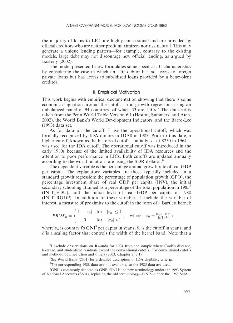
(INIT_EDU), and the initial level of real GDP per capita in 1988(INIT_RGDP). In addition to these variables, I include the variable ofinterest, a measure of proximity to the cutoff in the form of a Bartlett kernel:

PROXit ¼1� jzitj for jzitj � 1

0 for jzitj41; where zit ¼ ln yit�ln �yt

lnð1þbÞ :

(

where yit is country i’s GNI8 per capita in year t, �yt is the cutoff in year t, andb is a scaling factor that controls the width of the kernel band. Note that a

5I exclude observations on Rwanda for 1994 from the sample where Cook’s distance,leverage, and studentized residuals exceed the conventional cutoffs. For conventional cutoffsand methodology, see Chen and others (2003, Chapter 2, 2.1).

6See World Bank (2001) for a detailed description of IDA eligibility criteria.7The corresponding 1988 data are not available, so the 1985 data are used.8GNI is commonly denoted as GNP. GNI is the new terminology under the 1993 System

of National Accounts (SNA), replacing the old terminology—GNP—under the 1968 SNA.


657

negative coefficient for PROX implies that there is a negative relationshipbetween the country’s growth rate and its proximity to the cutoff. The scalingfactor, b, is set equal to 1

2, but I obtained similar results in the cases whereb¼ 1

3and b¼ 1

4. Appendix IV reports the distribution of PROX and partial

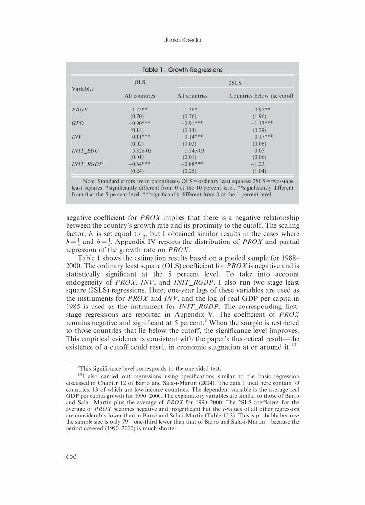
regression of the growth rate on PROX.Table 1 shows the estimation results based on a pooled sample for 1988–

2000. The ordinary least square (OLS) coefficient for PROX is negative and isstatistically significant at the 5 percent level. To take into accountendogeneity of PROX, INV, and INIT_RGDP, I also run two-stage leastsquare (2SLS) regressions. Here, one-year lags of these variables are used asthe instruments for PROX and INV, and the log of real GDP per capita in1985 is used as the instrument for INIT_RGDP. The corresponding first-stage regressions are reported in Appendix V. The coefficient of PROXremains negative and significant at 5 percent.9 When the sample is restrictedto those countries that lie below the cutoff, the significance level improves.This empirical evidence is consistent with the paper’s theoretical result—theexistence of a cutoff could result in economic stagnation at or around it.10

Table 1. Growth Regressions

Variables

OLS 2SLS

All countries All countries Countries below the cutoff

PROX �1.73** �1.38* �3.97**(0.70) (0.76) (1.96)

GPO �0.90*** �0.91*** �1.13***(0.14) (0.14) (0.29)

INV 0.11*** 0.14*** 0.17***

(0.02) (0.02) (0.06)

INIT_EDU �5.32e-03 �1.54e-03 0.05

(0.01) (0.01) (0.06)

INIT_RGDP �0.64*** �0.88*** �1.23(0.24) (0.25) (1.04)

Note: Standard errors are in parentheses. OLS=ordinary least squares; 2SLS=two-stageleast squares. *significantly different from 0 at the 10 percent level. **significantly differentfrom 0 at the 5 percent level. ***significantly different from 0 at the 1 percent level.

9This significance level corresponds to the one-sided test.10I also carried out regressions using specifications similar to the basic regression

discussed in Chapter 12 of Barro and Sala-i-Martin (2004). The data I used here contain 79countries, 13 of which are low-income countries. The dependent variable is the average realGDP per capita growth for 1990–2000. The explanatory variables are similar to those of Barroand Sala-i-Martin plus the average of PROX for 1990–2000. The 2SLS coefficient for theaverage of PROX becomes negative and insignificant but the t-values of all other regressorsare considerably lower than in Barro and Sala-i-Martin (Table 12.3). This is probably becausethe sample size is only 79—one-third fewer than that of Barro and Sala-i-Martin—because theperiod covered (1990–2000) is much shorter.

Junko Koeda

658

III. The Model

Official creditors typically fix their concessional interest rates; for example,the rates of the World Bank’s IDA and the IMF’s PRGF are 0.7511 and 0.5percent, respectively. I thus consider the following concessional lending rule:the lender who has full access to the world financial markets loans out fundsat a fixed subsidized interest rate (�r) as long as the country’s output per capita(y) is below the cutoff (�y).12 The interest rates for concessional lending arethus set according to the following rule:

~rtþ1 ¼�r if yt � �y;

r otherwise;

((1Þ

where r is the world interest rate. I assume that the borrower country has noaccess to foreign private financing, given that in practice, the majority ofloans to LICs are offered by official lenders.

In addition, I impose a participation constraint to motivate the borrowerto adhere to the contract.13 With this constraint, the borrower’svalue function under repayment is required to be greater than or equalto its value function under default. The borrower country solves thefollowing problem:

maxfct; ktþ1;Xtþ1g

X1t¼1

bt�1uðctÞ; (2Þ

subject to

vDðktÞ � uðctÞ þ bX1j¼1

bj�1uðctþjÞ 8t; (3Þ

ct ¼ f ðktÞ � xt þ Xtþ1=ð1þ ~rtþ1Þ � Xt; (4Þ

ktþ1 ¼ ð1� dÞkt þ xt; (5Þ

k1 andX1 are given; (6Þ

~rtþ1 follows the rule given byEquation ð1Þwith yt ¼ f ðktÞ; (7Þ

where c, x, k, and X denote consumption, investment, capital, and repaymentobligation, respectively. The repayment obligation in period t, Xt, is defined

11More precisely, this is the service charge that the World Bank currently imposes on theloans.

12The model assumes that the cutoff is expressed in terms of GDP per capita. In practice,however, it is defined in terms of GNI per capita, which excludes the interest payments onexternal debt from GDP. Appendix I presents the borrower’s problem where the cutoff isexpressed in terms of GNI per capita. The main conclusions hold true for the GNI case.

13The cases with no participation constraints are discussed in Appendix II.


659

by Xt¼ (1þ rt)Dt, where Dt is concessional debt due in period t.14 b is thediscount factor where r� 1/b�1 is assumed in order for consumption in thesteady state to be flat. The participation constraint is given by Equation (3).The LIC’s flow budget constraint is given by Equation (4). The productionfunction is given by f(kt). The transition equation for capital is given byEquation (5), where d is the rate of capital depreciation. The value functionunder default, vD(k), is the value function in autarky with penalties forviolating the participation constraint:

vDðkÞ ¼ maxk 0fuðð1� lÞf ðkÞ � k0 þ ð1� dÞkÞ þ bvDðk0Þg; (8Þ

where l is the fraction of output lost. I assume that such a violation incurstwo types of costs: the exclusion of the violator from future concessionallending and the loss of a fraction of the violator’s output. I also assume thatwhen the participation constraint is binding, the LIC adheres to theborrowing contract.

In each period, the borrower country compares the value function underrepayment, vR(k,X), with that under default, vD(k). When vR(k,X)ZvD(k) thecountry repays; otherwise it defaults. The value function under repayment,vR(.,.), is given by:

vRðk;XÞ ¼maxk 0;X 0

u f ðkÞ � k0 þ ð1� dÞkðf

þ X 0

ð1þ ~rðkÞÞ � X

�þ bvRðk0;X 0Þ

�; ð9Þ

subject to vRðk0;X 0Þ � vDðk0Þ; (10Þ

where vR(.,.) is increasing in k and is decreasing in X. Appendix III interpretsthe first-order conditions (FOCs) of the Bellman equation (equations (9) and(10)).

To make a connection with Cohen and Sachs’s model (1986), theparticipation constraint can be replaced with a debt capacity functionh(k),which is defined implicitly by vR(k, h)¼ vD(k), where qvR(k,X)/qX isstrictly negative. In other words, given k, h(k) is uniquely determined andthus the case where h(k) is backward bending in k can be excluded. Thus the

14The model is expressed with X rather than D, because otherwise the interest rates wouldbe a function of the previous period’s capital (call this k�1), and thus k�1 would need to betreated as an additional state variable in the model’s recursive equation.

Junko Koeda

660

debt capacity function is well defined. The original value function underrepayment can be rewritten as



þminX 0

ð1þ ~rðkÞÞ ;hðk0Þ

ð1þ ~rðkÞÞ

� �� X

�þ bvRðk0;X 0Þ

�: ð11Þ

This formulation is the same as that of Cohen and Sachs (1986),15 exceptthat in this paper I numerically derive the value functions and the implieddebt capacity function using the value function iteration method.16 I alsoextend their model to analyze the dynamics of concessional loans to LICs.

IV. The Numerical Results

Because one cannot solve this problem analytically unless the participationconstraint is absent, I solve it numerically using the value function iterationmethod. I specify the functional forms of the utility and production functionsas u(c)¼ c1�1/s/(1�1/s) and f(k)¼AkZ.

Calibration

Table 2 lists calibrated parameter values. Depreciation of capital is set at0.1—a reasonable number in the real business cycle literature (for example,see Kydland and Prescott, 1982). The concessional interest rate is set at 0.75percent, in line with existing official concessional lending practice. The valueof the capital elasticity of the production function (Z¼ 0.33) is based on thefindings in Gollin (2002) and is consistent with the existing real business cycleliterature. The paper’s main results are robust to alternative values of Z¼ 0.3and 0.4; a poverty trap arises with Z¼ 0.2 if there is a slight change in otherparameter values.

The discount factor is set at 0.95 and the world interest rate at1/b�1¼ 0.0526 in order to obtain flat consumption in the steady state. Debtoverhang emerges more easily with a smaller value of b (or a higher r)because the borrower country will have a stronger incentive to consume inearlier periods (or because the benefits from concessional loans are larger).With a higher value of b, a poverty trap arises if there is a slight change inother parameter values.

The value for the elasticity of intertemporal substitution (s¼ 0.45) is inline with the calibration results of Ogaki, Ostry, and Reinhart (1996). Using

15An extension of Cohen and Sachs (1986) can be seen in Borensztein and Ghosh’s (1989)mode.

16Here, I use a two-period utility function (that is, u(c)þ bu(c0)) and an arbitrary debtcapacity function (that is, h(k, r)¼ constant) as the starting functions; if the participationconstraint is violated, the utility function is penalized. I obtain the same fixed point in thefunctional space.


661

Cooley and Ogaki’s (1996) two-step procedure,17 they estimate the lower andupper bounds of the intertemporal elasticity of substitution assuming that theelasticity is an increasing function of the level of wealth.18 The paper’s mainconclusions are robust to alternative values of s¼ 1

3and 2

3if there is a slight

change in other parameter values.The fraction of output lost on default (l) is set at 0.05. This value needs

to be sufficiently positive to maintain the paper’s main conclusions. If it iszero, then there will be no default cost in the steady state and thus theborrower country will have an incentive to default; as a result, no loans willbe made.

The cutoff level (�y) is set as a fraction of steady-state output in the UnitedStates (yUS). I use 0.15, because the purchasing-power-parity-adjusted realoutputs per capita in most lower-middle-income countries are above thislevel. I calculate yUS by omitting the participation constraint and byassuming that U.S. TFP is 30 (note: this number is just a scaling factor) andthe LIC-U.S. TFP ratio is 1

3.19 The paper’s main conclusions are sensitive to

the LIC’s steady-state output level relative to the cutoff. More details arediscussed at the end of this section.

Benchmark Economy

Consider the benchmark economy with initial income (y1) equal to 90 percentof the cutoff (or about 70 percent of steady-state output (yss)), and initialdebt repayment obligation (X1) equal to 90 percent of the cutoff (or 100percent of y1).

Table 2. Calibrated Parameter Values

Depreciation rate of capital (d) 0.1000 Elasticity of intertemporal

substitution (s)0.45

Concessional interest rate (�r) 0.0075 Fraction of output lost on

default (l)0.05

Capital elasticity of output (Z) 0.3300 Cutoff level (fraction of U.S.

steady-state output)

0.15

Time preference (b) 0.9500 Level of TFP for the U.S. 30.00

Note: TFP=total factor productivity.

17Following this two-step procedure, they first estimate the intratemporal parameters in atwo-good model of tradable and non-tradable goods. Given these intratemporal parameters,they then estimate the intertemporal elasticity of substitution by applying the generalizedmethod of moments to the Euler equation.

18Atkeson and Ogaki (1996) show that the intertemporal elasticity of substitution riseswith the level of wealth.

19A cursory glance at the TFP ratio of 40 LICs relative to the United States between 1960and 2000 shows that about one-fourth of LICs have TFP levels that are less than one-third theU.S. level and are stable.

Junko Koeda

662

Figures 1 and 2 summarize the results from the numerical solution. Tobetter understand the dynamics of concessional lending, these results aredisplayed along with those for nonconcessional lending. The only differencebetween these two loans is the interest rate level, where r¼ r for all t undernonconcessional loans. Thus, the nonconcessional debt capacity functionhN(k) is defined implicitly by vR(k, hN)¼ vD(k), where qvR(k,X)/qX is strictlynegative and r¼ r for all t.

This discontinuity of the concessional debt capacity function (h(k))20

implies that the recipient country must drastically reduce its external debtprecisely when it surpasses the cutoff. Such debt reduction is possible onlythrough a steep decline in consumption, which the country may find too

Figure 1. The Benchmark Economy: Numerical Results

Output Consumption

0 5 10 15 20 25 30 35

0.6

0.7

0.8

0.9

1

(in years)0 5 10 15 20 25 30 35

0.4

0.5

0.6

0.7

0.8

0.9

(in years)

Investment Repayment Obligation

0 5 10 15 20 25 30 350

0.1

0.2

0.3

0.4

0.5

(in years)0 5 10 15 20 25 30 35

0.7

0.8

0.9

1

1.1

(in years)

Note: Panels (a)–(d) show how the benchmark economy will respond under the concessionallending (solid line) and nonconcessional lending (dotted line) schemes. The paths of output,consumption, investment, and repayment obligation are shown as a fraction of the steady-stateoutput level (yss).

20This discontinuity emerges in the amount of resources that can be borrowed (h(k)/(1þ rtþ 1)) as a result of the jump in the interest rate that takes place as soon as the country’sincome exceeds the cutoff.


663

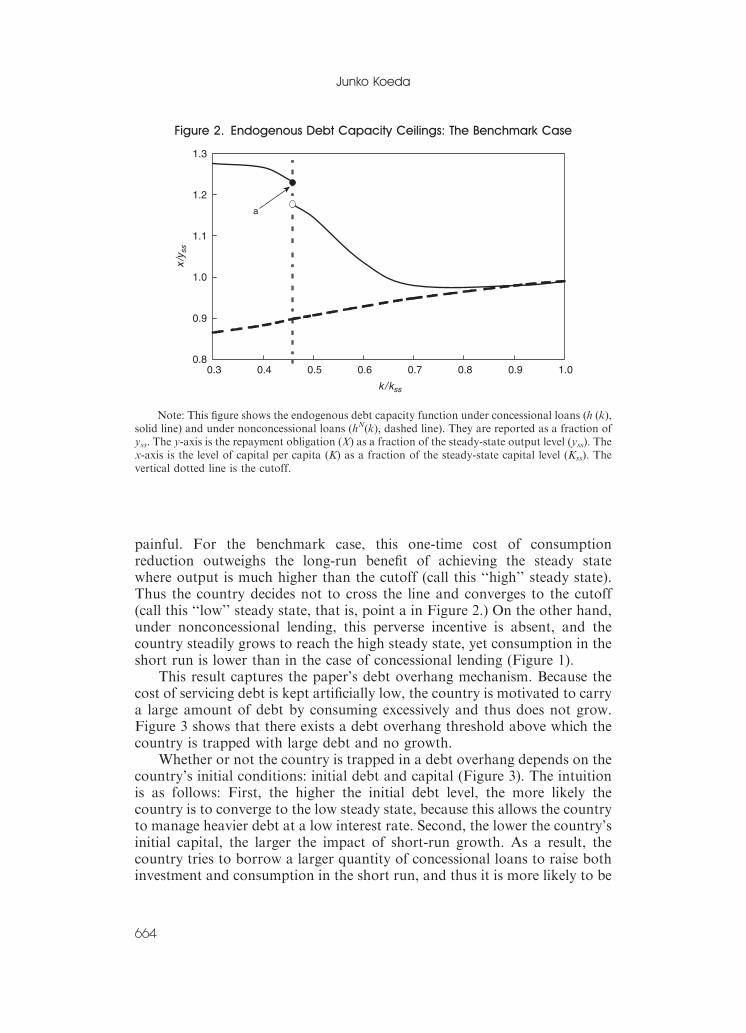
painful. For the benchmark case, this one-time cost of consumptionreduction outweighs the long-run benefit of achieving the steady statewhere output is much higher than the cutoff (call this ‘‘high’’ steady state).Thus the country decides not to cross the line and converges to the cutoff(call this ‘‘low’’ steady state, that is, point a in Figure 2.) On the other hand,under nonconcessional lending, this perverse incentive is absent, and thecountry steadily grows to reach the high steady state, yet consumption in theshort run is lower than in the case of concessional lending (Figure 1).

This result captures the paper’s debt overhang mechanism. Because thecost of servicing debt is kept artificially low, the country is motivated to carrya large amount of debt by consuming excessively and thus does not grow.Figure 3 shows that there exists a debt overhang threshold above which thecountry is trapped with large debt and no growth.

Whether or not the country is trapped in a debt overhang depends on thecountry’s initial conditions: initial debt and capital (Figure 3). The intuitionis as follows: First, the higher the initial debt level, the more likely thecountry is to converge to the low steady state, because this allows the countryto manage heavier debt at a low interest rate. Second, the lower the country’sinitial capital, the larger the impact of short-run growth. As a result, thecountry tries to borrow a larger quantity of concessional loans to raise bothinvestment and consumption in the short run, and thus it is more likely to be

Figure 2. Endogenous Debt Capacity Ceilings: The Benchmark Case

0.8

0.9

1.0

1.1

1.2

1.3

0.3 0.4 0.5 0.6 0.7 0.8 0.9 1.0

x/y

ss

k /kss

a

Note: This figure shows the endogenous debt capacity function under concessional loans (h (k),solid line) and under nonconcessional loans (hN(k), dashed line). They are reported as a fraction ofyss. The y-axis is the repayment obligation (X) as a fraction of the steady-state output level (yss). Thex-axis is the level of capital per capita (K) as a fraction of the steady-state capital level (Kss). Thevertical dotted line is the cutoff.

Junko Koeda

664

trapped in the low steady state. In short, the country converges to the highsteady state only if initial debt is low enough, initial income is high enough,or both conditions hold.

Whether or not the country is trapped in a debt overhang is alsoconditional on the country’s TFP level (Figure 4). The higher the TFP, thehigher the steady-state output level relative to the cutoff, and therefore thegreater the long-run benefit of achieving the high steady state. With a higherTFP, the country thus finds it more costly to be trapped in the low steadystate. Figure 4 shows that the debt overhang threshold shifts up with a higherTFP level. With a higher TFP level, the country is more likely to lie below thedebt overhang threshold. Note that here the initial income level is kept thesame across different TFP levels; initial capital levels are adjustedaccordingly.

V. Policy Implications and Conclusions

Implications for Aid Design

Even though the paper does not solve for the most efficient form of aid,21 itdoes have implications for aid design. First, the model implies that the

Figure 3. The Debt Overhang Threshold and Initial Conditions

0.0

0.5

1.0

1.5

0.80 0.85 0.90 0.95 1.00 1.05 1.10

Initial income/cutoff

A

B

C D

EF

BenchmarkIn

itial

rep

aym

ent o

blig

atio

n/cu

toff

Note: This figure shows a debt overhang threshold (solid) above which a country is trappedwith large debt and no growth. It shows that if the country lies in region A or B, it converges to thelow steady state, whereas if it lies in C or D, it achieves the high steady state. Arrears countries thatlie above these ceilings (E and F) are outside the scope of this paper. The y-axis is the initialrepayment obligation as a fraction of the cutoff. The x-axis is the initial income as a fraction of thecutoff. The dash-dotted line is the endogenous debt capacity ceilings. The vertical dotted line is thecutoff.

21For more discussion towards an optimal debt relief proposal see, for example, Rajan(2005).


665

perverse incentive arising from per capita income eligibility exists under otherforms of aid as well. For example, if a country repeatedly receives sufficientlylarge grants with a similar income per capita eligibility criterion, it may havean incentive to stagnate around the cutoff in order to maintain future granteligibility.

Second, the model suggests that the existing eligibility and allocationrules could take into account other aspects, in addition to income per capita,in order to avoid the perverse incentive. In practice, some measures of TFPare already taken into account in the aid allocation formula of themultilateral development banks. For example, the IDA Country Policy andInstitutional Assessment takes into account policy and structural indicators.

Third, the model implies that certain forms of graduation policies mayprovide stronger growth incentives as well as reduce the cost of aidassistance. For example, the model’s debt overhang may disappear if theconcessional interest rates are allowed to increase with income levels. Thisimplies that a more gradual move from concessional to nonconcessionallending provides the right incentive for growth. Indeed, the existence of‘‘blend countries’’ suggests that something is at work in IDA and othermultilateral development banks’ operational rules.

Implications for Debt Relief

The model implies that a one-time-debt-relief stock treatment may beeffective in helping a country get out of the poverty trap and achieve growth.

Figure 4. Debt Overhang Thresholds with Different TFPs

0.0

0.5

1.0

1.5

0.80 0.85 0.90 0.95 1.00 1.05 1.10Initial Income/Cutoff

Benchmark

TFP level is 1% higher than the bechmark

Debt overhang thresholds

Debt capacity celilings

Initi

al r

epay

men

t obl

igat

ion/

cuto

ff

Note: The solid lines show the endogenous debt capacity ceilings and debt overhang thresholdusing the benchmark parameter values. The dotted lines show the corresponding figures when thetotal factor productivity (TFP) level is 1 percent higher than the benchmark economy. The y-axis isthe size of the initial repayment obligation as a fraction of the cutoff. The x-axis is the initial incomeas a fraction of the cutoff. The vertical dotted line is the cutoff.

Junko Koeda

666

For example, suppose that the benchmark economy receives one-time reliefthat enables the country to move below the debt overhang threshold (solidline in Figure 3). The country now converges to the high steady state.

One-time debt relief may also be effective even if the country initially liesabove the cutoff. Consider a country that has relatively high initial debtand lies in region B in Figure 3. Note that this country has an incentive to goback to the cutoff because the benefit of raising the debt ceiling by reducingcapital is greater than the cost of lowering output. The country is thusbetter off reducing output until it eventually falls to the cutoff. Here upfrontdebt relief that moves the country from B to D is effective in achievinggrowth.

Note that if such a stock treatment is accompanied by factors thatcan raise TFP, such as productivity growth and an improvement ininstitutional quality, then the debt overhang threshold itself will shiftupward (Figure 4) resulting in a larger number of countries that lie below thethreshold. This means that if debt relief resources are used for developmentpurposes that also directly raise TFP, more countries will be able to achievegrowth given the same amount of debt relief. The above argumentsprovide some justification for the recent one-time-debt-relief stocktreatment, known as the Multilateral Debt Relief Initiative (MDRI). TheMDRI is a 100 percent debt stock cancellation by the IMF, the IDA, andthe African Development Bank for a group of LICs; its goal is to free upresources to help countries achieve the United Nations’ MillenniumDevelopment Goals.

However, there are some caveats to this argument. First, for this type ofstock treatment to work, it is important that recipient countries view itas a one-time event. If they do not, the poverty trap may reemerge ifcountries receive repeated debt relief with similar income per capita eligibilitycriteria. Second, the theoretical environment may be too efficient; that is,the model assumes that the country can efficiently reallocate freed resourcesfrom debt relief to productive activities. In reality, however, it may be quitedifficult to handle a sudden increase in resources in the presence of weakinstitutions.

Conclusions

Whether an LIC is trapped in a debt overhang depends on its initialconditions and its TFP. The larger the initial debt, the stronger the incentivesan LIC has to manage its debt at a low interest rate by becomingpermanently aid dependent. The lower an LIC’s initial income, the more ittries to borrow a larger quantity of concessional loans to raise bothinvestment and consumption in the short run and thus becomes more likelyto be trapped in the low steady state. Last, the lower the level of TFP, themore likely it becomes that the benefit of remaining at the cutoff exceeds thelong-run benefit of achieving the high steady state.


667

APPENDIX I

Per Capita Income Cutoff: GDP vs. GNI

The model defines the cutoff in terms of GDP per capita. However, in practice, it is

defined in terms of GNI per capita, which excludes the interest payments on external debt

from GDP. Because a high level of external debt alters the level of capital stock above

which the country loses eligibility, this new feature introduces an additional incentive for

debt accumulation. However, as shown below, the paper’s key conclusion—a poverty

trap occurs depending on the country’s TFP and initial conditions—still holds under the

GNI case. This appendix solves a borrower’s problem in which the country’s output per

capita is expressed in terms of GNI per capita—more specifically, it solves the problem of

Equations (2)–(7) with y now defined as y¼ f(k)�rX/(1þ r).

The Bellman equation now has three state variables because rtþ 1 becomes a function

of rt as well as kt and Xt:

vRðk;X ; ~rÞ ¼maxk 0;X 0

u f ðkÞ � k0 þ ð1� dÞkþ X 0

ð1þ ~r0Þ � X

� ��

þbvRðk0;X 0; ~r0Þ�; ðA:1Þ

Figure A1. The Benchmark Economy with a GNI per Capita Cutoff: Numerical Results

Output Consumption

0 5 10 15 20 25 30 35

0.7

0.8

0.9

1

(in years)0 5 10 15 20 25 30 35

0.4

0.5

0.6

0.7

0.8

0.9

(in years)

Investment Repayment Obligation

0 5 10 15 20 25 30 350

0.1

0.2

0.3

0.4

0.5

(in years)0 5 10 15 20 25 30 35

0.7

0.8

0.9

1

1.1

(in years)

Note: Panels (a)–(d) show how the benchmark economy will respond under the concessionallending (solid line) and nonconcessional lending (dotted line) schemes. The paths of output,consumption, investment, and repayment obligation are shown as a fraction of the steady-stateoutput level (yss).

Junko Koeda

668

subject to vR(k0,X0, r 0)ZvD(k0), where r0 follows the rule given by Equation (1) and

is equal to �r if f(k)�rX/(1þ r)r�y, and r otherwise. The debt capacity function

h(k, r ) is defined implicitly by vR(k, h, r)¼ vD(k), where qvR(k,X, r)/qX is strictly

negative.

I numerically solve for two value functions, vR(k,X,�r) and vR(k,X, r), because rt can

take only two values, �r and r. I solve these functions in the same manner as in Section IV

using the same parameter values and functional forms. The numerical results for the

benchmark economy (see Appendix Figures A1 and A2) are very similar to those

presented in Section IV.

In the GNI case, however, the corresponding endogenous debt capacity function is

more complicated than Figure 2 in the text. Lines Fr and F�r are the graphs of X¼ ((1þ r )/

r )(f(k)��y), where r is equal to r and �r, respectively. These lines determine the interest rate

in the next period; for example, if rt¼�r, then rtþ 1¼ r if the country lies on the right-hand

side of the line F�r, and rtþ 1¼�r otherwise. kr and k�r are the levels of capital at the points of

discontinuity for h(k, r) and h(k,�r), respectively. k is the level of capital that satisfies�y¼AkZ.

Could a poverty trap still occur in the GNI case? Yes. Suppose the country initially

lies at point (a) in Appendix Figure A2 with r1¼�r. This implies that the interest rate in

period 2 is also �r, because the point (k1,X1) lies on the left-hand side of the line F�r. If the

country chooses to cross k�r in period 2, the point (k2,X2) will lie on the right-hand side of

the line F�r. Here, consumption in period 2 must be very low, because the country needs to

reduce borrowing. This is the same story discussed in Section IV.

Figure A2. Endogenous Debt Ceilings with a GNI per Capita Cutoff:The Benchmark Case

0.0

0.2

0.4

0.6

0.8

1.0

1.2

1.4

0.3 0.4 0.5 0.6 0.7 0.8 0.9 1.0

k/kss

X/y

ss

k rk

h(k,r)/yss

h(k,r)/yss

FrrF

b

c

rk

a

Note: The solid lines show the endogenous debt capacity ceilings under concessional loans(h(k, r )), and the dashed line shows those ceilings under nonconcessional loans (h(k)). They areshown as a fraction of the steady-state output level (yss). The y-axis is the repayment obligation (X)as a fraction of yss. The x-axis is capital per capita (k) as a fraction of the steady-state capital level(kss). There are three vertical lines: the left line is the cutoff and the middle and right (kr and k�r) showthe levels of capital at the points of discontinuity for h(k, r) and h(k,�r), respectively. The dotted lines(Fr and F�r) are the graphs of X¼ ((1þ r)/r)(f(k)��y) where r is equal to r and �r, respectively.


669

The new feature of the GNI case can be demonstrated as follows. Suppose the country

initially lies on the right-hand side of the line Fr, say at point (b), with r1¼ r. This implies

that the interest rate in period 2 is also r. Here, the country could significantly increase its

borrowing and consumption in period 2—for example, by moving to point (c)—as long

as the point (k2,X2) remains at or below h(k, r). However, this implies that the country

would need to move back below h(k,�r) in period 3, which requires consumption in that

period to be very low. As a result, the country would not choose to converge to point

(kr, h(kr, r)), that is, the point of discontinuity of h(k, r).

Oscillating solutions, in which the country chooses to move back and forth between

the right- and left-hand sides of the line Fr, could also occur, depending on the initial

conditions. This is because under the GNI cutoff rule, the problem has multiple

discontinuities, as shown in the figure.

APPENDIX II

No Participation Constraints

This appendix considers the environment in which the LIC fully precommits to honoring

the conditions of the concessional lending scheme that is imposed by the creditor so that

there is no need to impose a participation constraint. In practice, though, this is an

unrealistic assumption because it allows the LIC unlimited access to the donor’s funds.

Analyzing this nonparticipation constraint environment, however, is nonetheless useful

to understand the role of a debt ceiling constraint.

In the absence of participation constraints, capital overshoots in period 1 as a result of

a subsidized interest rate. The problem is given by

maxct;ktþ1

X1t¼1

bt�1uðctÞ:

Subject to the intertemporal budget constraint

f ðk1Þ þ ð1� dÞk1 þX1t¼2

Pt

s¼2

1

1þ ~rs

� �ðf ðktÞ þ ð1� dÞktÞ

� �

¼ ð1þ ~r1ÞD1 þ c1 þ k2 þX1t¼2

Pt

s¼2

1

1þ ~rs

� �ðct þ ktþ1Þ

� �;

where K1, D1, and r1 are given. FOCs are given by

u0ðctÞ ¼ m for t ¼ 1; (A:2Þ

bt�1u0ðctÞ ¼ mYts¼2

1

1þ ~rs

� �for t � 2; (A:3Þ

~rtþ1 ¼ f 0ðktþ1Þ � d for t � 1; (A:4Þwhere m is the shadow price. Initially, the country can borrow at the concessional interest

rate (that is, r2¼�r) because I assume that initial output lies below the cutoff. At any level

of capital above the cutoff, the country can borrow only at the world interest rate. The

capital levels in period 2 and in the steady state, k2 and kss, are pinned down by�r¼ f0(k2)�d and r¼ f0(kss)�d (by equation (A.4)). These equations imply that k2 is greater

than kss because the concessional interest rate is lower than the world interest rate (�ror).

Junko Koeda

670

Thus capital overshoots the steady state in period 1. However, from period 3 onward,

capital is at its steady-state level (that is, kj¼ kss for jZ3), because as of period 2, the

country no longer has access to concessional loans. Its capital level exceeds the cutoff,

and the capital level is kss (from equation (A.4)). Consumption, too, overshoots in period

1 (c1>c2¼ css). This is implied by the following Euler equations: u0(c1)¼b(1þ�r)u0(c2)and u0(c2)¼ b(1þ r)u0(c3), because b(1þ�r)o1, b(1þ r)¼ 1, and u0(c) is decreasing in c.

Once {k2, kss} and {c1, css} are pinned down, the path of debt, {D2,Dss} can be derived via

the budget constraint. The dynamics of concessional loans without a participation

constraint are thus characterized by the overshooting of capital and consumption in

period 1 as a result of the low concessional interest rate. The donor’s budget, a, is

determined by a�D2(r��r)/(1þ r).

APPENDIX III

The FOCs of the Bellman Equation

The Bellman equation (equations (9) and (10)) can be rewritten as Equations (A.5) and

(A.6)



þ X 0

ð1þ ~rðkÞÞ � X

�þ bvRðk0;X 0Þ

�; ðA:5Þ

subject toX 0 � hðk0Þ; (A:6Þbecause vR(k0,X0)ZvD(k0) and X0rh(k0) are equivalent by construction, given the debt

capacity function. In the following, I consider two cases: X0oh(k0) and X0 ¼ h(k0), andinterpret the corresponding FOCs.

CASE 1: X0oh(k0)The FOC with respect to k0 is given by uc(c )¼bv k

R(k0, X 0 ), and by the envelope

theorem, vkR(k,X)¼ uc(c)(fk(k)þ 1�d).

The Euler equation is given by

ucðcÞ ¼ bucðc0Þðfkðk0Þ þ 1� dÞ: (A:7ÞThe FOC with respect to X0 is given by �uc(c)/(1þ r(k,X))¼ bvx

R(k0,X0), and by the

envelope theorem, vXR(k,X)¼�uc(c). Combining the above two equations we get

ucðcÞ ¼ bð1þ ~rðk;XÞÞucðc0Þ: (A::8ÞEquation (A.8) can be rewritten as uc(c)¼b(1þ�r)uc(c

0) if the country lies strictly

below the cutoff, and uc(c)¼b(1þ r)uc(c0) if the country lies strictly above the cutoff.

Because b(1þ�r)ob(1þ r)¼ 1, the country has an incentive to overconsume in earlier

periods under the concessional lending scheme.

CASE 2: X 0 ¼ h (k0)The Bellman equation (equations (A.5) and (A.6)) can be rewritten as



þ hðk0Þð1þ ~rðkÞÞ � X

�þ bvRðk0; hðk0ÞÞ

�:


671

The FOC with respect to k0 is given by

ucðcÞ 1� hkðk0Þ1þ ~rðkÞ

� �¼ b½vRk ðk0; hðk0ÞÞ þ vRX ðk0; hðk0ÞÞhkðk0Þ�

and by the envelope theorem, vkR(k,X)¼ uc(c)(fk(k)þ 1�d), and vX

R(k,X)¼�uc(c). Thusthe Euler equation is given by

ucðcÞ 1� hkðk0Þ1þ ~rðkÞ

� �¼ bucðc0Þðfkðk0Þ � hkðk0Þ þ 1� dÞ: (A:9Þ

The numerical simulations suggest that h(.,.) is decreasing in k unless the country lies

sufficiently above the cutoff. Thus there is upward pressure for c, whereas there is

downward pressure for c0—the country has an incentive to overconsume around the

cutoff in earlier periods. To state this intuition more formally, rewrite Equation (A.9) as

ucðcÞ ¼ b1þ ~rðkÞ

1þ ~rðkÞ � hkðk0Þucðc0Þ½fkðk0Þ þ 1� d� hkðk0Þ�: (A:10Þ

One can interpret the bracketed term as the return from savings. The term b(1þ r(k))/

(1þ r(k)�hk(k0)) can be interpreted as the effective discounting factor. If h(.,.) were

constant so that hk(.,.) would be zero, then Equation (A.10) would reduce to the familiar

expression with the return from savings given by fk(k0)þ 1�d and the discounting factor

given by b. The implication of the downward-sloping h (that is, hk(.,.)o0) is twofold.

First, the return from capital, the bracketed term in Equation (A.10), is suppressed.

Second, the ratio in Equation (A.10) is less than 1, which effectively lowers the discount

rate. Both effects act to depress savings.

APPENDIX IV

A Description of PROX

There are more than 1,300 observations on PROX between 1987 and 2000, of which

about 17take positive values (that is, only 1

7of the observations lie close to the cutoffs).

Appendix Figure A3 shows the histogram of PROX excluding observations with

PROX¼ 0. When I carry out a simple OLS regression of the growth rate of real GDP per

capita on PROX, the coefficient for PROX is negative (�2.22) and is statistically

significant at 1 percent.

Appendix Figure A4 relates the growth rate with the level of GNI after removing

regressors other than PROX. Recall that the empirical model is y¼ cþaPROXþ gZþ e,where y is the percentage per capita annual growth rate of real GDP, PROX is a measure

of proximity to the cutoff, and Z represents the other explanatory variables. Denote c, a,and g as the OLS coefficients. Appendix Figure A4 plots the OLS residuals of the growth

rate excluding aPROX (that is, y�c�gZ) and aPROX against the percentage deviation of

GNI from the threshold for IDA eligibility.

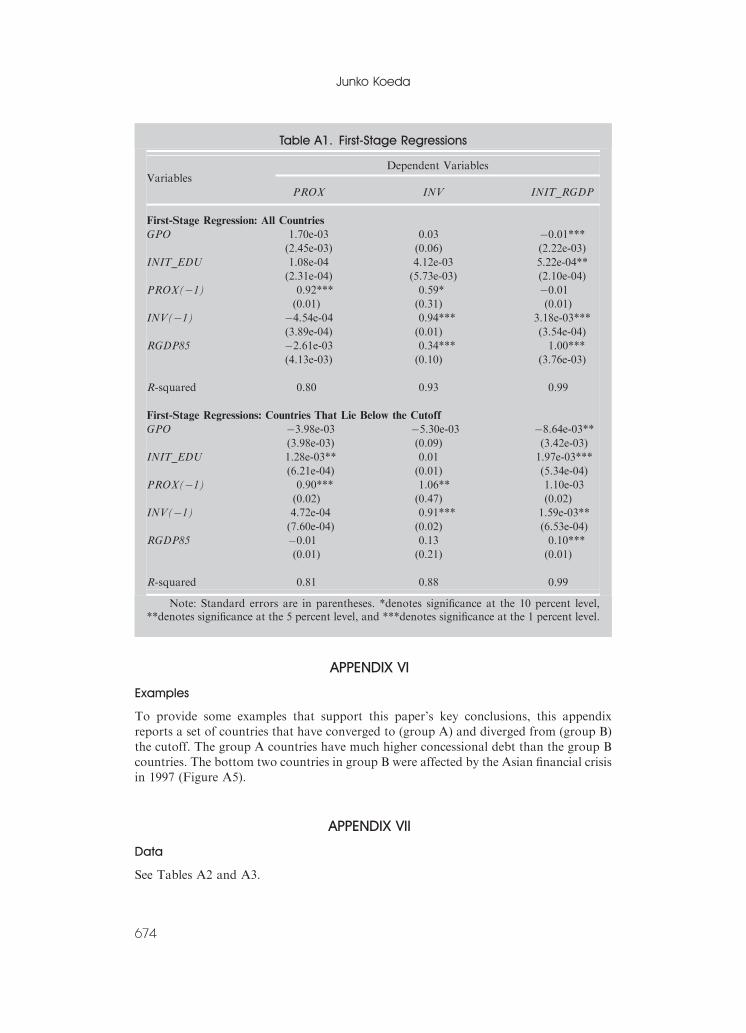
APPENDIX V

First-Stage Regressions

See Table A1.

Junko Koeda

672

Figure A3. Frequency of PROX

0

0.5

1

1.5

2

Den

sity

0 0.2 0.4 0.6 0.8 1

PROX

Note: This figure reports the histogram of PROX excluding observations with PROX¼ 0.

Figure A4. Ordinary Least Square Residuals Excluding alpha hat*PROX

-20

-15

-10

-5

0

5

10

15

20

-50 -30 -10 10 30 50

• residuals excluding alpha_hat*PROX

Note: Remember that the paper’s empirical model is y¼ cþ aPROXþ gZþ e, where y is thepercent annual growth rate of real GDP per capita, PROX is a measure of proximity to the cutoff,and Z represents the other explanatory variables. Denote c, a, and g as the OLS coefficients. Thefigure plots the ordinary least squares (OLS) residuals of the growth excluding aPROX (that is,y�c�gZ) and aPROX against the deviation of GNI from the threshold for IDA eligibility.


673

APPENDIX VI

Examples

To provide some examples that support this paper’s key conclusions, this appendix

reports a set of countries that have converged to (group A) and diverged from (group B)

the cutoff. The group A countries have much higher concessional debt than the group B

countries. The bottom two countries in group B were affected by the Asian financial crisis

in 1997 (Figure A5).

APPENDIX VII

Data

See Tables A2 and A3.

Table A1. First-Stage Regressions

VariablesDependent Variables

PROX INV INIT_RGDP

First-Stage Regression: All Countries

GPO 1.70e-03 0.03 �0.01***(2.45e-03) (0.06) (2.22e-03)

INIT_EDU 1.08e-04 4.12e-03 5.22e-04**

(2.31e-04) (5.73e-03) (2.10e-04)

PROX(�1) 0.92*** 0.59* �0.01(0.01) (0.31) (0.01)

INV(�1) �4.54e-04 0.94*** 3.18e-03***

(3.89e-04) (0.01) (3.54e-04)

RGDP85 �2.61e-03 0.34*** 1.00***

(4.13e-03) (0.10) (3.76e-03)

R-squared 0.80 0.93 0.99

First-Stage Regressions: Countries That Lie Below the Cutoff

GPO �3.98e-03 �5.30e-03 �8.64e-03**(3.98e-03) (0.09) (3.42e-03)

INIT_EDU 1.28e-03** 0.01 1.97e-03***

(6.21e-04) (0.01) (5.34e-04)

PROX(�1) 0.90*** 1.06** 1.10e-03

(0.02) (0.47) (0.02)

INV(�1) 4.72e-04 0.91*** 1.59e-03**

(7.60e-04) (0.02) (6.53e-04)

RGDP85 �0.01 0.13 0.10***

(0.01) (0.21) (0.01)

R-squared 0.81 0.88 0.99

Note: Standard errors are in parentheses. *denotes significance at the 10 percent level,**denotes significance at the 5 percent level, and ***denotes significance at the 1 percent level.

Junko Koeda

674

Figure A5. Examples

-100

0

100

200

300

400

500

1987 1989 1991 1993 1995 1997 1999-100

0

100

200

300

400

1987 1989 1991 1993 1995 1997 1999

-60

-40

-20

0

20

40

60

1987 1989 1991 1993 1995 1997 1999-40

-20

0

20

40

60

80

1987 1989 1991 1993 1995 1997 1999

0

20

40

60

80

100

120

140

1987 1989 1991 1993 1995 1997 19990

20406080

100120140160

Group B: Countries That Have Diverged from the Cutoff

1987 1989 1991 1993 1995 1997 1999

0

50

100

150

200

250

1987 1989 1991 1993 1995 1997 1999-10

0

10

20

30

40

1987 1989 1991 1993 1995 1997 1999

Group A: Countries That Have Converged to the Cutoff

Source: World Bank, Global Development Finance.Note: The dashed lines report concessional loans as a percent of GNI between 1987 and 2000

for countries that have converged to the cutoff (Group A) and that have diverged from the cutoff(Group B). The solid lines show the percent deviations from the per capita income cutoffs.


675

Table A2. Data

Variables Definition Source

Growth rate The growth rate of real GDP per

capita (in percent)

Constructed from real GDP per capita,

Constant prices: Laspeyres (RGDPL)

in Summers-Heston data set, version

6.1

GNI GNI per capita in current U.S.

dollars, Atlas methodology

World Development Indicators

�y The operational IDA cutoff in terms

of GNI per capita in U.S. dollars,

Atlas methodology

World Bank GNI/capita operational

guidelines

GPO Percent population growth (a year) Constructed from population (POP) in

Heston, Summers, and Aten, 2002

INV Investment share of real GDP per

capita (in percent a year)


INIT_RGDP The log of real GDP per capita in

1985, constant prices: Laspeyres


INIT_EDU Percent of secondary schooling

attained in the total population in

1985

Barro-Lee data set

Note: IDA=World Bank International Development Association.

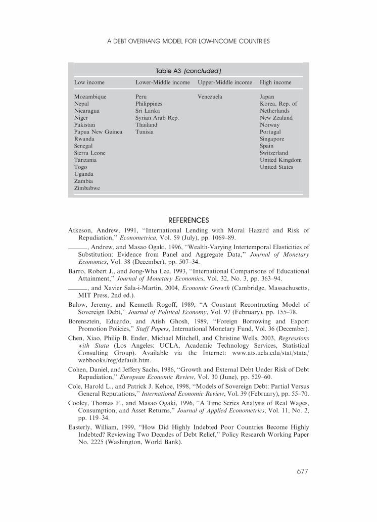
Table A3. Country or Regional Coverage of the Data Set

Low income Lower-Middle income Upper-Middle income High income

Bangladesh Algeria Argentina Australia

Benin Bolivia Barbados Austria

Cameroon Brazil Botswana Belgium

Central African Rep. Dominican Rep. Chile Canada

Congo, Dem. Rep. of Ecuador Costa Rica Cyprus

Congo, Rep. of El Salvador Hungary Denmark

Gambia, The Fiji Malaysia Finland

Ghana Guatemala Mauritius France

Guinea-Bissau Guyana Mexico Germany

Haiti Honduras Poland Greece

India Indonesia Panama Hong Kong SAR

Kenya Iran, I.R. of South Africa Iceland

Lesotho Jamaica Trinidad and Tobago Ireland

Malawi Jordan Turkey Israel

Mali Paraguay Uruguay Italy

Junko Koeda

676

REFERENCESAtkeson, Andrew, 1991, ‘‘International Lending with Moral Hazard and Risk of

Repudiation,’’ Econometrica, Vol. 59 (July), pp. 1069–89.

_______, Andrew, and Masao Ogaki, 1996, ‘‘Wealth-Varying Intertemporal Elasticities ofSubstitution: Evidence from Panel and Aggregate Data,’’ Journal of MonetaryEconomics, Vol. 38 (December), pp. 507–34.

Barro, Robert J., and Jong-Wha Lee, 1993, ‘‘International Comparisons of EducationalAttainment,’’ Journal of Monetary Economics, Vol. 32, No. 3, pp. 363–94.

_______, and Xavier Sala-i-Martin, 2004, Economic Growth (Cambridge, Massachusetts,MIT Press, 2nd ed.).

Bulow, Jeremy, and Kenneth Rogoff, 1989, ‘‘A Constant Recontracting Model ofSovereign Debt,’’ Journal of Political Economy, Vol. 97 (February), pp. 155–78.

Borensztein, Eduardo, and Atish Ghosh, 1989, ‘‘Foreign Borrowing and ExportPromotion Policies,’’ Staff Papers, International Monetary Fund, Vol. 36 (December).

Chen, Xiao, Philip B. Ender, Michael Mitchell, and Christine Wells, 2003, Regressionswith Stata (Los Angeles: UCLA, Academic Technology Services, StatisticalConsulting Group). Available via the Internet: www.ats.ucla.edu/stat/stata/webbooks/reg/default.htm.

Cohen, Daniel, and Jeffery Sachs, 1986, ‘‘Growth and External Debt Under Risk of DebtRepudiation,’’ European Economic Review, Vol. 30 (June), pp. 529–60.

Cole, Harold L., and Patrick J. Kehoe, 1998, ‘‘Models of Sovereign Debt: Partial VersusGeneral Reputations,’’ International Economic Review, Vol. 39 (February), pp. 55–70.

Cooley, Thomas F., and Masao Ogaki, 1996, ‘‘A Time Series Analysis of Real Wages,Consumption, and Asset Returns,’’ Journal of Applied Econometrics, Vol. 11, No. 2,pp. 119–34.

Easterly, William, 1999, ‘‘How Did Highly Indebted Poor Countries Become HighlyIndebted? Reviewing Two Decades of Debt Relief,’’ Policy Research Working PaperNo. 2225 (Washington, World Bank).

Table A3 (concluded )

Low income Lower-Middle income Upper-Middle income High income

Mozambique Peru Venezuela Japan

Nepal Philippines Korea, Rep. of

Nicaragua Sri Lanka Netherlands

Niger Syrian Arab Rep. New Zealand

Pakistan Thailand Norway

Papua New Guinea Tunisia Portugal

Rwanda Singapore

Senegal Spain

Sierra Leone Switzerland

Tanzania United Kingdom

Togo United States

Uganda

Zambia

Zimbabwe


677

_______, 2002, The Elusive Quest for Growth: Economists’ Adventures and Misadventures inthe Tropics (Cambridge, Massachusetts, MIT Press).

Eaton, Jonathan, and Raquel Fernandez, 1995, ‘‘Sovereign Debt,’’ NBER Working PaperNo. 5131 (Cambridge, Massachusetts, National Bureau of Economic Research).

_______, and Mark Gersovitz, 1981, ‘‘Debt with Potential Repudiation: Theoretical andEmpirical Analysis,’’ Review of Economic Studies, Vol. 48, pp. 289–309.

Gollin, Douglas, 2002, ‘‘Getting Income Shares Right,’’ Journal of Political Economy,Vol. 110 (April), pp. 458–74.

Heston, Alan, Robert Summers, and Bettina Aten, 2002, ‘‘Penn World Table Version6.1,’’ Center for International Comparisons at the University of Pennsylvania(Philadelphia, University of Pennsylvania). Available via the Internet:pwt.econ.upenn.edu/php_site/pwt_index.php.

International Monetary Fund, 2003, ‘‘Debt Sustainability in Low-Income Countries—Towards a Forward-Looking Strategy’’ (Washington). Available via the Internet:www.imf.org/external/np/pdr/sustain/2003/052303.pdf.

_______, and World Bank, 2004, ‘‘Debt Sustainability in Low-Income Countries: FurtherConsiderations on an Operational Framework and Policy Implications,’’(Washington). Available via the Internet: www.imf.org/external/np/pdr/sustain/2004/091004.htm.

_______, ‘‘Operational Framework for Debt Sustainability Assessments in Low-IncomeCountries—Further Considerations,’’ (Washington). Available via the Internet:www.imf.org/External/np/pp/eng/2005/032805.pdf.

_______, 2006, ‘‘Review of Low-Income Country Debt Sustainability Framework andImplications of the MDRI,’’ (Washington). Available via the Internet: www.imf.org/external/np/pp/eng/2006/032406.pdf.

Krugman, Paul, 1988, ‘‘Financing vs. Forgiving a Debt Overhang,’’ Journal ofDevelopment Economics, Vol. 29 (November), pp. 253–68.

Kydland, Finn E., and Edward C. Prescott, 1982, ‘‘Time to Build and AggregateFluctuations,’’ Econometrica, Vol. 50 (November), pp. 1345–70.

Ogaki, Masao, Jonathan D. Ostry, and Carmen M. Reinhart, 1996, ‘‘Saving Behavior inLow- and Middle-Income Developing Countries: A Comparison,’’ IMF Staff Papers,Vol. 43 (March).

Rajan, Raghuram, 2005, ‘‘Straight Talk: Debt Relief and Growth,’’ Finance &Development, Vol 42 (June).

Rose, Andrew K, 2005, ‘‘One Reason Countries Pay Their Debts: Renegotiation andInternational Trade,’’ Journal of Development Economics, Vol. 77 (June), pp. 189–206.

Sachs, Jeffrey, 1989, ‘‘The Debt Overhang of Developing Countries,’’ in DebtStabilization and Development: Essays in Memory of Carlos Diaz Alejandro, ed. byGuillermo Calvo and others (Oxford, Basil Blackwell).

World Bank, 2001, IDA Eligibility, Terms, and Graduation Policies (Washington, WorldBank).

Yue, Vivian Z., 2006, ‘‘Sovereign Default and Debt Renegotiation’’ (New York: NewYork University, unpublished). Available via the Internet: www.econ.nyu.edu/user/yue/Yue_2006.pdf.

Junko Koeda

678

a debt overhang model for low-income countries · pdf filea debt overhang model for low-income...

Documents