a dipole model for high energy qcd - …home.thep.lu.se/~leif/misc/thesis.pdf · a dipole model for...
TRANSCRIPT

A DIPOLE MODEL
FOR HIGH ENERGY QCD
Christoffer Flensburg
Department of Theoretical PhysicsLund University
Thesis for the degree of Doctor of Philosophy
Thesis Advisor: Leif LonnbladFaculty Opponent: Raju Venugopalan
To be presented, with the permission of the Faculty of Science of LundUniversity, for public criticism in lecture hall F of the Department ofPhysics on Friday, the 29th of April 2011, at 10.15.

ii
DO
KU
MEN
TD
ATABLAD
enlSIS
61
41
21
Organization
LUND UNIVERSITYDepartment of Theoretical PhysicsSolvegatan 14ASE–223 62 LUNDSwedenAuthor(s)
Christoffer Flensburg
Document name
DOCTORAL DISSERTATIONDate of issue
March 2011Sponsoring organization
Title and subtitle
A Dipole Model for High Energy QCD
Abstract
This thesis considers a model of high energy particle collisions. The model is basedon the so called BFKL formalism which is valid only at low x, that is collisions atvery high energies, such as at the LHC. The intial state of the incoming particlesare simulated by colour dipoles in transverse space evolved through rapidity. Withthis approach, all fluctuations are dynamically described, allowing for a large set ofobservables to be calculated.The first paper compares the model to experimental results and the model is found todescribe a large set of experiments with pp and γ∗p accurately with just four tunableparameters. The second paper studies the fluctuations in the interaction probability,and how this affects the cross section for diffractive excitation in pp and γ∗p. Themodel is further compared to a different approach, and many similarities are noted.The third paper studies the correlations between multiple hard subscatterings in ppwhich are important for finding new physics at LHC.The fourth paper is the largest project, and introduces a full event generator basedon the dipole model. Here the dipoles are not only tracked in the initial evolution,but also all the particles coming out from the collision are calculated. It is foundto provide a competetive description of all minimum bias data, something that hasnever been done in the BFKL formalism before. This provies a good comparison forother event generators that normally use a different approach.
Key words:
QCD, Phenomenology, Dipole Model, low x
Classification system and/or index terms (if any):
Supplementary bibliographical information: Language
English
ISSN and key title: ISBN
978-91-7473-112-5
Recipient’s notes Number of pages
190Price
Security classification
Distributor
Christoffer FlensburgDepartment of Theoretical Physics, Solvegatan 14A, SE–223 62 Lund, SwedenI, the undersigned, being the copyright owner of the abstract of the above-mentioned dissertation, hereby grant toall reference sources the permission to publish and disseminate the abstract of the above-mentioned dissertation.
Signature Date 2011-03-24

A DIPOLE MODEL
FOR HIGH ENERGY QCD
Christoffer Flensburg
Department of Theoretical PhysicsLund University

ii
Copyright © Christoffer Flensburg
Department of Theoretical Physics, Lund UniversityISBN 978-91-7473-112-5
Printed in Sweden by Media-Tryck, Lund UniversityLund 2011

iii
Sammanfattning
Fysiker forsoker beskriva verkligheten. Idag finns det en beskrivningsom forklarar i stor utstrackning det vi ser omkring oss, fran solensenergikalla och himlens farg, till atomers uppbyggnad och universumsminsta bestandsdelar. Beskrivningen kan sammanfattas i en ekvationpa ett par rader, och kallas for Standardmodellen, och inkluderas harhuvudsakligen av estetiska skal:
L = iψ /Dψ + ψiyijψjφ + h.c.
− 1
4FµνFµν +
∣
∣Dµφ∣
∣
2 − V(ψ)
Standardmodellen beskriver de minsta bestandsdelarna: materie-partiklarna, och de kraftbarande partiklarna. Den beskriver hur ett fatalpartiklar interagerar med varandra, och man kan utifran det i principbeskriva situationer med hur manga partiklar som helst. I praktiken blirdock matematiken snabbt for komplicerad om man forsoker att direktlosa standardmodellens ekvationer for manga partiklar, och man kaninte langre gora exakta forutsagelser
For att avgora om det ar en bra beskrivning sa behover den jamforasmed verkligheten; teorin behover jamforas med experiment. Sa for atttesta standardmodellen mot sa manga experiment som mojligt, ar detviktigt att rakna ut forutsagelser for sa manga scenarier som mojligt.I de flesta fall ar det omojligt att rakna ut en exakt forutsagelse,och det ar nodvandigt att infora approximationer och forenklingar iberakningarna.
For att undersoka Standardmodellen sa direkt som mojligt, anvandsofta experiment med partikelacceleratorer, dar man accelererar partiklar(som till exempel elektroner eller protoner) till hog hastighet, kolliderardem, och ser hur de interagerar. I det fallet ar det i allmanhet bara ettfatal partiklar inblandade i kollisionen, vilket gor det mojligt att goraforutsagelser. Standardmodellen stammer mycket val overens med des-sa experiment, vilket bekraftar att det ar en bra modell.
Det ar inte alltid enkelt att gora forutsagelser for partikelkollisioner;detta galler speciellt nar det ar protoner som kolliderar, som ar falletvid den nybyggda acceleratorn LHC: Large Hadron Collider, i Geneve.En proton ar inte en elementarpartikel, utan ar uppbyggd av tre mindrepartiklar som kallas kvarkar. En kvark ar en av elementarpartiklarna istandardmodellen, och ar en del av all materia vi har omkring oss. De
iv
tre kvarkarna i en proton halls ihop av en kraft som kallas “den star-ka kraften”. Detta sker genom att de hela tiden skickar gluoner mellanvarandra, dar gluonerna ar de kraftbarande partiklarna for den starkakraften. Detta gor att nar en proton accelereras och kolliderar, sa ar detinte en ensam partikel som kolliderar, utan det ar tre kvarkar tillsam-mans med en mangd gluoner. Detta gor det mer komplicerat att raknaut vad som hander nar tva protoner kolliderar.
Dessutom interagerar gluonerna med varandra, vilket gor situatio-nen annu mer komplicerad. Aven om en proton borjar som tre kvarkar,sa kommer den i varje ogonblick ocksa ha nagra gluoner, lat oss sagatva stycken, som skickas mellan kvarkarna. Det forandrar nu situatio-nen igen, eftersom gluonerna kan skicka ut ytterligare gluoner mellanvarandra. Sa de tre kvarkarna och tva gluonerna kommer ha ytterligaregluoner mellan sig, som i sin tur orsakar annu fler gluoner och sa vida-re. Den har sjalvforstarkande kaskaden av gluoner ar kraftigare ju merenergi protonerna kolldierar med.
Sa nar tva protoner kolliderar ar det egentligen tva kaskader av kvar-kar och gluoner som krashar in i varandra, och ju hogre energi de kroc-kar med, desto fler kvarkar och gluoner ar det som kolliderar. Detta armycket komplicerat att rakna ut direkt fran standardmodellen. Vid kol-lisioner med tillrackligt hog energi finns det dock en forenkling av stan-darmodellen, som kallas BFKL-ekvationen, som mojliggor berakningarav den inkommande kaskaden av kvarkar och gluoner.
Jag har i mitt doktorandarbete utgatt fran BFKL-ekvationen och ut-vecklat en model som simulerar de inkommande kaskaderna av kvar-kar och gluoner, och som darmed kan beskriva mycket av det somhander i kollisioner, till exempel vid LHC.
Var losningsansats ar att utga fran kvarkarna och sedan med hjalpav en dator simulera en gluon i taget som skickas ut fran de foregaendepartiklarna, och i varje ny utskickad gluon ta hansyn till sa mycket de-taljer som mojligt. Pa sa satt kan vi fa en mycket mer detaljerad bild avhur de kolliderande kaskaderna ser ut an vad som har gjorts tidigare.
Nar de tva kaskaderna kolliderar och kvarkarna och gluonerna far utfran kollisionen sa galler andra regler, och var model kan inte anvandaslangre. Det finns dock andra forenklingar som beskriver de utgaendepartiklarna val, och vi har kombinerat var model med andra tidigaremodeller for att kunna fortsatta att beskriva vad som hander med kaska-derna aven efter kollisionen. Pa det sattet har vi byggt upp en sa kalladhandelsegenerator, som simulerar hela processen fran de forsta inkom-mande kvarkarna, genom kaskaden innan kollision, interaktionen med

v
den andra kaskaden och interaktioner pa vagen ut fran kollisionen, helavagen till de partiklar som till slut kommer ut fran kollisioner.
En sadan kaskad fran handelsegeneratorn finns illustrerad langst nertill hoger pa varje uppslag, och genom att bladdra igenom hornet pa allasidorna snabbt kan man se tva protoner vid LHC rora sig mot varandraoch kollidera. Protonerna beskrivs av de tre kvarkarna, sammankopp-lade av “dipoler” som representerar gluonerna som hela tiden skickasfram och tillbaka. Efter hand som fler och fler gluoner skickas ut kom-mer det fler och fler dipoler som kopplar ihop de nya gluonerna.
I till exempel LHC mats dessa utgaende partiklarna, och vi kanjamfora resultaten fran vara simuleringar med experiment. Standard-modellen ar inte en “Teori for Allting”, utan vi vet att det maste finnasnagot mer, om inte annat sa ingar inte gravitation. Genom att battreforsta vad vi vantar oss fran standardmodellen kan vi enklare se teckenpa om nagot nytt behovs.

vi
This thesis is based on the following publications:
I Christoffer Flensburg, Gosta Gustafson and Leif Lonnblad,Elastic and quasi-elastic pp and γ⋆p scattering in the Dipole
Model
European Physics Journal C60 (2009) 233-247 e-Print:[arXiv:0807.0325].
II Christoffer Flensburg and Gosta GustafsonFluctuations, Saturation, and Diffractive Excitation in High
Energy Collisions
Journal of High Energy Physics 1010 (2010) 014 e-Print:[arXiv:1004.5502].
III Christoffer Flensburg, Gosta Gustafson, Leif Lonnblad and An-dras Ster,Correlations in double parton distributions at small xLU-TP 11-12CERN-PH-TH-2011-059MCnet-11-09e-Print: [arXiv:1103.4320].
IV Christoffer Flensburg, Gosta Gustafson and Leif Lonnblad,Inclusive and Exclusive observables from dipoles in high energy
collisions
LU-TP 11-13CERN-PH-TH-2011-058MCnet-11-08e-Print: [arXiv:1103.4321].

vii
Contents
i Introduction 1
i.1 Particle Physics: history up to today . . . . . . . . . . . 1
i.1.1 The atom . . . . . . . . . . . . . . . . . . . . . . 2i.1.2 The atom as electrons and nucleus . . . . . . . 3
i.1.3 The nucleus as protons and neutrons . . . . . . 4i.1.4 The protons and neutrons as quarks . . . . . . 6
i.1.5 The properties of the forces . . . . . . . . . . . 8i.1.6 The standard model . . . . . . . . . . . . . . . . 9
i.1.7 The strong force at hadron colliders . . . . . . . 10i.2 Mathematical foundation . . . . . . . . . . . . . . . . . 12
i.2.1 The observables . . . . . . . . . . . . . . . . . . 12
i.2.2 Feynman diagrams, and calculating a cross sec-tion . . . . . . . . . . . . . . . . . . . . . . . . . 13
i.2.3 QCD, not so simple . . . . . . . . . . . . . . . . 14
i.2.4 BFKL: a high energy approximation . . . . . . 16i.3 The Lund Dipole Model: my contribution . . . . . . . . 17
i.3.1 Our model . . . . . . . . . . . . . . . . . . . . . 18i.3.2 Further applications . . . . . . . . . . . . . . . . 21
i.3.3 Future development . . . . . . . . . . . . . . . . 23i.4 Introduction to papers . . . . . . . . . . . . . . . . . . . 24
i.4.1 Paper I: Elastic and quasi-elastic pp and γ⋆pscattering in the Dipole Model . . . . . . . . . . 24
i.4.2 Paper II: Fluctuations, Saturation, and Diffrac-tive Excitation in High Energy Collisions . . . . 25
i.4.3 Paper III: Correlations in double parton distri-butions at small x . . . . . . . . . . . . . . . . . 25
i.4.4 Paper IV: Inclusive and Exclusive observablesfrom dipoles in high energy collisions . . . . . 26
i.4.5 List of contributions . . . . . . . . . . . . . . . . 26i.5 A PhD defence for a non-physicist . . . . . . . . . . . . 27
i.5.1 The schedule . . . . . . . . . . . . . . . . . . . . 27i.5.2 What to do during the defence? . . . . . . . . . 28

viii
Acknowledgments . . . . . . . . . . . . . . . . . . . . . 29References . . . . . . . . . . . . . . . . . . . . . . . . . . 30
I Elastic and quasi-elastic pp and γ⋆p scattering in the Dipole
Model 33
I.1 Introduction . . . . . . . . . . . . . . . . . . . . . . . . . 34I.2 Formalism . . . . . . . . . . . . . . . . . . . . . . . . . . 36
I.2.1 The dipole cascade model and the eikonal ap-proximation . . . . . . . . . . . . . . . . . . . . 36
I.2.2 DVCS and exclusive vector meson productionin γ∗p collisions . . . . . . . . . . . . . . . . . . 37
I.2.3 Differential cross sections . . . . . . . . . . . . . 38I.3 The improved dipole cascade . . . . . . . . . . . . . . . 39
I.3.1 Non-leading perturbative effects . . . . . . . . 39
I.3.2 Saturation within the cascades . . . . . . . . . . 40I.3.3 Confinement effects . . . . . . . . . . . . . . . . 41
I.4 Initial wave functions . . . . . . . . . . . . . . . . . . . 42
I.4.1 Proton wave function . . . . . . . . . . . . . . . 42I.4.2 Photon wavefunction . . . . . . . . . . . . . . . 44
I.4.3 Meson wavefunctions . . . . . . . . . . . . . . . 46I.5 Tuning of parameters and the differential pp cross section 49
I.5.1 The total and elastic pp cross section . . . . . . 49
I.5.2 The differential elastic pp cross section . . . . . 52I.5.3 The total γ⋆p cross section and tuning the pho-
ton wave function . . . . . . . . . . . . . . . . . 53I.6 Results for quasi-elastic γ⋆p collisions . . . . . . . . . . 55
I.6.1 Deeply Virtual Compton Scattering . . . . . . . 55I.6.2 Exclusive Production of Light vector Mesons . 56I.6.3 Exclusive ψ Production . . . . . . . . . . . . . . 60
I.7 Conclusions and Outlook . . . . . . . . . . . . . . . . . 61References . . . . . . . . . . . . . . . . . . . . . . . . . . 64
II Fluctuations, Saturation, and Diffractive Excitation in High
Energy Collisions 69
II.1 Introduction . . . . . . . . . . . . . . . . . . . . . . . . . 70II.2 The eikonal approximation and the Good–Walker for-
malism . . . . . . . . . . . . . . . . . . . . . . . . . . . . 72
II.2.1 Eikonal approximation . . . . . . . . . . . . . . 72II.2.2 Good–Walker formalism . . . . . . . . . . . . . 73II.2.3 What are the diffractive eigenstates? . . . . . . 74

ix
II.3 The dipole cascade model . . . . . . . . . . . . . . . . . 74II.3.1 Mueller’s dipole model . . . . . . . . . . . . . . 74
II.3.2 The Lund dipole cascade model . . . . . . . . . 76II.3.3 Application to diffraction . . . . . . . . . . . . . 79
II.4 The nature of the fluctuations and effects of saturation 82
II.4.1 γ∗p scattering . . . . . . . . . . . . . . . . . . . 82II.4.2 pp scattering . . . . . . . . . . . . . . . . . . . . 84
II.5 Impact parameter profile and t-dependence in pp-collisions . . . . . . . . . . . . . . . . . . . . . . . . . . . 86
II.6 Relation Good–Walker – Triple-Regge . . . . . . . . . . 88
II.7 Conclusions . . . . . . . . . . . . . . . . . . . . . . . . . 93II.8 Acknowledgements . . . . . . . . . . . . . . . . . . . . 94
References . . . . . . . . . . . . . . . . . . . . . . . . . . 95
III Correlations in double parton distributions at small x 99
III.1 Introduction . . . . . . . . . . . . . . . . . . . . . . . . . 100
III.2 Double Parton Scattering and Double Parton Distribu-tions . . . . . . . . . . . . . . . . . . . . . . . . . . . . . 102III.2.1 Experimental results . . . . . . . . . . . . . . . 102III.2.2 Formalism . . . . . . . . . . . . . . . . . . . . . 103
III.2.3 Correlations . . . . . . . . . . . . . . . . . . . . 104III.3 The Lund Dipole Cascade Model . . . . . . . . . . . . . 107
III.3.1 Mueller’s dipole cascade . . . . . . . . . . . . . 107
III.3.2 The Lund dipole cascade model . . . . . . . . . 108III.4 Application to double parton distributions . . . . . . . 111III.5 Results . . . . . . . . . . . . . . . . . . . . . . . . . . . . 112
III.5.1 Subcollisions at midrapidity . . . . . . . . . . . 112
III.5.2 Sub-collisions off midrapidity . . . . . . . . . . 114III.5.3 Comparison with experiment . . . . . . . . . . 115III.5.4 Comment on the definition of b . . . . . . . . . 117
III.6 Conclusions and outlook . . . . . . . . . . . . . . . . . . 117References . . . . . . . . . . . . . . . . . . . . . . . . . . 121
IV Inclusive and Exclusive observables from dipoles in high en-
ergy collisions 125
IV.1 Introduction . . . . . . . . . . . . . . . . . . . . . . . . . 126IV.2 The Lund dipole cascade model for inclusive cross sec-
tions . . . . . . . . . . . . . . . . . . . . . . . . . . . . . 128IV.2.1 Mueller’s cascade model and the eikonal for-
malism . . . . . . . . . . . . . . . . . . . . . . . 128

x
IV.2.2 The Lund dipole cascade model . . . . . . . . . 131IV.2.3 Initial dipole configurations . . . . . . . . . . . 133
IV.3 From inclusive to exclusive observables . . . . . . . . . 133IV.3.1 The chain of k⊥-changing gluons . . . . . . . . 133IV.3.2 Reabsorption of virtual emissions . . . . . . . . 134IV.3.3 Giving proper weights to the emissions . . . . 135IV.3.4 Going from transverse coordinate space to mo-
mentum space . . . . . . . . . . . . . . . . . . . 138IV.3.5 Final state radiation and hadronization . . . . . 140
IV.4 Generating the exclusive final states . . . . . . . . . . . 140IV.4.1 Selecting the interactions . . . . . . . . . . . . . 141IV.4.2 Identifying the backbone gluons . . . . . . . . . 142IV.4.3 Reweighting outer q⊥ maxima . . . . . . . . . . 142IV.4.4 FSR matching and ordering . . . . . . . . . . . 143IV.4.5 Colour flow . . . . . . . . . . . . . . . . . . . . 144IV.4.6 Higher order corrections . . . . . . . . . . . . . 144
IV.5 Self-consistency and tuning . . . . . . . . . . . . . . . . 146IV.5.1 Achieving frame independence . . . . . . . . . 146IV.5.2 Tuning to experimental data . . . . . . . . . . . 150IV.5.3 Comparison with experiments . . . . . . . . . . 152
IV.6 Conclusions and outlook . . . . . . . . . . . . . . . . . . 157IV.A q⊥ max reweighting in DIPSY . . . . . . . . . . . . . . . 161IV.B Absorbed partons and ordering . . . . . . . . . . . . . . 163
IV.B.1 Coherence . . . . . . . . . . . . . . . . . . . . . 164IV.B.2 Ordering in the interaction . . . . . . . . . . . . 166
IV.C Saturation effects . . . . . . . . . . . . . . . . . . . . . . 168IV.C.1 Multiple interaction . . . . . . . . . . . . . . . . 169IV.C.2 The Swing . . . . . . . . . . . . . . . . . . . . . 169IV.C.3 colour flow in saturated cascades . . . . . . . . 171References . . . . . . . . . . . . . . . . . . . . . . . . . . 173

i
Introduction
This introduction will have readers ranging from interested friendsand family without background in physics, through undergraduate andgraduate physics students, to the referees and opponent with decades ofexperience in particle physics research. I have tried to dedicate at leasta few pages to every possible level of the reader, but let me warn you,the reader, that you will find part of the introduction too trivial, or tooinvolved.
Non-physicists will probably find section i.1 the most interesting,with a historical introduction leading up to todays situation of particlephysics, and description of the problems and solutions that this thesisaddresses. If you are reading this at the defence, you should considerskipping ahead to section i.5 for an explanation of what is going on, andhow you can make the most of it.
Section i.2 introduces particle physics in a more mathematical way,as well as the basic concepts that form the foundation of my research.
Section i.3 goes into more detail of the work, and assumes some ex-perience from particle physics, and in section i.4 the publications aresummarised.
i.1 Particle Physics: history up to today
The first mentions of matter being built up of some smallest object, anelementary particle, trace back to around 600 B.C. in ancient India andGreece, where the word “atomos”, meaning unsplittable, was coined.At that time there was however no experiment capable of supporting orrejecting this idea, and the concept could not be developed very far.
i
2 Introduction
i.1.1 The atom
The first elementary particle model with experimental support was Dal-ton’s atomic theory in early 19:th century, describing early chemistry interms of elementary particles. One of the strong experimental supportsfor this theory was the law of multiple proportions.
The law of multiple proportions Oxygen and carbon can combinein two ways: either each carbon atom pairs up with each oxygenatom forming CO, the toxic gas carbon monoxide, or each carbonatom pairs up with two oxygen atoms, forming CO2, carbon diox-ide that help plants transform sunlight into chemical energy (andrecently maybe more known from global warming contexts).
Splitting up 1 kg of carbon monoxide in oxygen and carbon, youwill get as many carbon atoms as oxygen atoms, but as the oxygenatom is a heavier by 33%, you will get 429 grams of carbon, and571 grams of oxygen, that is, 1.33 times as much oxygen as carbonin weight.
Repeating the experiment with 1 kg of carbon dioxide, splittingit up in carbon and oxygen, you will get double the number ofoxygen atoms, meaning 273 grams of carbon and 727 grams ofoxygen. That is, 2.66 times as much oxygen as carbon.
The ratio in the second experiment, 2.66, is exactly the double of1.33 in the first experiment. Today we know that this is becauseeach carbon atom in CO2 is coupled with 2 oxygen atoms, whileCO is coupled to only one, but to the chemists in early 19:th cen-tury found this property very curious, and it was an importantreason for John Dalton to formulate his atomic theory.
Not everyone believed that the success that Dalton’s atomic theory hadin explaining experiments meant that all matter really was built up oftiny elementary particles, but saw it more as a mathematical trick. Amore direct observation was the analysis of Brownian motion.
Brownian motion Water is made of a very small water moleculesthat moves around in the liquid. If a sufficiently small object isplaced in the water, it will feel the individual collisions with thewater molecules, and will be bouncing around randomly from thecollisions, even if initially left at rest. An example of this kind ofmotion, Brownian motion, is shown in figure i.1.
Robert Brown was in 1827 observing pollen grains in water with a mi-croscope, and saw small pieces of the grains break off and move arounderratically and randomly. Brown reported the observation, but it wasnot until the end of the 19:th century, or even beginning of 20:th, that

i.1 Particle Physics: history up to today 3
Figure i.1: Brownian motion. The lines describes the motion of a dust particlein for example water. The black line is measuring at longer time intervals,while the blue lines measure the position more frequently.
a mathematical explanation in terms of atoms was made, confirmingDalton’s theory.
i.1.2 The atom as electrons and nucleus
While most matter is formed from atoms, the atoms are not elementaryparticles, in the sense that they are not unsplittable. It was known that aneutral atom can give off a negative electric charge, and the atom itselfwill get a positive charge. This is what happens for example with staticelectricity built up from rubbing a balloon on hair.
In 1897, J.J. Thomson showed that the negative electric charge is ac-tually a very light particle, now known as the electron. This was doneby stripping negative charge of atoms (like when rubbing a balloon)and then sending the charges through vacuum to a positive charge (forexample the sweater you just rubbed the balloon against). It turnedout that putting an object in the path of the negative charges stoppedthem from arriving to the positive charge, and it was concluded that thenegative charges were carried by some type of particle that got namedelectron. It was realised that the atom contains electrons, which were as-
i

4 Introduction
sumed to be floating around in a positively charged “pudding”. So theatom was seen as a pudding with the small electrons in it like raisinsand the picture got named the “plum pudding model”.
Soon after though, another experiment would again change how theatom was seen. Ernest Rutherford decided in 1909 to shoot alpha raysat a very thin gold foil. Alpha rays were seen as helium atoms strippedof both of their electrons, that is just the pudding part of the atom in theplum pudding model. The purpose was to study how the helium pud-ding would break up on the gold atoms, but to Rutherfords surprise,some of the alpha particles bounced back out almost the same way asthe came from. This was as surprising as throwing a cream cake at abrick wall, and see it bounce off it completely intact like a tennis ball.
The explanation was that the positive charge in an atom was notspread out, but concentrated in a small nucleus in the centre of the atom,that also would have most of the mass of the atom. The electrons weresuggested to rotate around this nucleus, similar to how the planets ro-tate around the sun, but rather than gravity keeping the planets to stayaround the sun, it would be the electromagnetic attraction between thepositively charged nucleus and the negatively charged electrons thatkept the atom together.
i.1.3 The nucleus as protons and neutrons
As the atom has a neutral charge in total, the amount of positive chargeof the nucleus determines how many electrons it would collect arounditself, and the number of electrons would determine the chemical prop-erties of the atom. So it was understood that there was one nucleus foreach kind of atom, distinguished by their charge and their mass.
In 1913, isotopes were discovered, that is, two nuclei with the samecharge, but with different masses. Further it was discover that themasses of the different isotopes, the different nuclei, increased in stepsof the same size.
The mass of a nucleus Today the atomic nucleus is understood asa compound of positively charged protons, and uncharged neu-trons, both with a mass of about 1.7 · 10−24 g. Although this maynot seem very heavy, this means that more than 99.9% of the massof an atom is concentrated in the nucleus, which is less than 0.01%of the diameter of the electron orbits.
For some reason physicists like to compare particles to fruits andvegetables, and following that convention, the relation in size anweight can be illustrated as follows: If the nucleus has the size and

i.1 Particle Physics: history up to today 5
Figure i.2: An atom. The nucleus contains protons and neutrons, and theelectrons orbit the nucleus. Not to scale: as the orbits are about 100,000 timesthe size of the nucleus, the nucleus would be just a fraction of a pixel in thispicture.
mass of a watermelon in the city centre of Lund, then the electronswould have the mass of peas, and the orbit would be covering thebigger part of Lund.
That said, as the nucleus is built of protons and neutrons with thesame mass, the total mass of a nucleus will be a whole numbertimes that mass. For example an oxygen nucleus has 8 protons(setting the electric charge of the nucleus to +8), and in general 8neutrons. As the proton and neutron masses are almost the same,this would put the total mass close to 16 times the mass of theproton. Similarly, a carbon nucleus will most often have a mass12 times that of the proton and so on, but one will never find anucleus with the mass of 16.5 times the proton mass.
Scientists found this too much to be a coincidence, and by 1932 the nu-cleus was described as a set of protons and neutrons, both with aboutthe same mass.
While the electrons were kept in place by the electromagnetic attrac-tion between the positive nucleus and the negative electrons, there wasno clear answer to what held the protons and neutrons together in thenucleus. In fact, the positively charged protons confined in such a smallvolume as the nucleus would push each other away very strongly. The
i

6 Introduction
conclusion was that there must be some other, even stronger, force thatkept the neutrons and protons together. This somewhat mysteriousforce was named, in lack of better suggestions, “the strong force”. Itshould here be mentioned that much of todays particle physics, includ-ing the thesis you are currently reading, is about understanding exactlyhow the strong force works.
i.1.4 The protons and neutrons as quarks
Around 1950 technical developed had reached the point where the firstparticle accelerators were built, propelling electrons, protons and neu-trons to almost the speed of light. Most of these experiments includedcrashing the particles into something at high speed, and in these colli-sions, many new particles were found. The new particles had similarmasses to the protons and neutrons, none as light as the electron, andall of them were interacting using the strong force. As the particles wereaccelerated to higher and higher speed (particle physicists usually say“to higher energy”), hundreds of new particles were found, to the ex-tent that the situation was referred to as a “particle zoo”. All of thesestrongly interacting particles, the neutron and the proton, plus all thenew ones, were called “hadrons”.
As happened with Dalton in discovering the law of multiple propor-tions, and as in the case with masses of the isotopes, also in this par-ticle zoo, some systems and regularities were found. While they werenot as straightforward regularities as the two examples mentioned, theystill pointed towards the hadrons being built up from smaller particles,called “quarks”. Scientists welcomed the effort to find some order in thezoo, but without more direct proof of the existence of quarks, the ideadid not get accepted immediately.
Hadrons from quarks Today we know that there are six differ-ent flavours (yes, physicists actually call them flavours) of quarks.However, only the two lightest flavours, the “up” quark and the“down” quark, are light enough to appear naturally. The other 4flavours are only seen in high energy particle collisions.
Each of the six flavours come in 3 different colours (again, yes,they are actually referred to as colours): red, green and blue.Quarks can be combined to form hadrons in any way, as long asthey combine in a colour-neutral way. This works in the same wayas real-life colours do, that is, red green and blue can combine togive white. “Colour-neutral” means that the quarks have to com-bine in a way that results in the colour white.

i.1 Particle Physics: history up to today 7
Figure i.3: How matter is built as we see it today. The atom is electrons orbitingthe nucleus, which is built from protons and neutrons, which in turn are builtfrom quarks.
A proton for example is built up from three quarks, two up quarks,and one down quark. Of these three quarks, there is one red,one blue and one green. Similarly for neutrons, which are builtfrom one up quark and two down quarks, but still with one ofeach colour. By combining the different flavours in different ways,and with different colour combination, the particle zoo of the hun-dreds of different hadrons is formed.
Recall Rutherford and his experiment with the gold foil and the heliumnuclei. He though he was colliding plum pudding, but he saw colli-sions as if he was hitting something very small and very heavy. Nowwe know that this very small and very heavy thing was the nucleus ofthe atom, and it is indeed much smaller than the atom (recall the water-melon analogy).
A similar experiment was done with the proton. There were theoriessaying that the proton was built up by smaller quarks, and one wouldbe able to see the internal structure if one collided it with somethingsufficiently hard. Luckily, by 1968 the technical development since thefirst accelerators had arrived at a point where this could be done, andindeed, in what was called “deep inelastic scattering”, one could seethe substructure of the proton. And while there were some difficultiesin confirming that this substructure actually was originating from thequarks suggested to explain the zoo, the model with the flavoured andcoloured quarks eventually got widely accepted.
i

8 Introduction
i.1.5 The properties of the forces
This is how we see the structure of matter today: The quarks are heldtogether by the strong force to form hadrons. The only two hadronsseen in the nature: the proton and the neutron, form the nucleus whilethe electrons orbit the nucleus, together being the atom. Thus the ele-mentary particles building up matter are the quarks and the electrons.
However, to understand nature, it is not enough to know its buildingblocks, one also has to understand how they interact with each other.We know today that each force is mediated through a force carrier, asort of particle, but a different kind of particle than the electrons andquarks which build up matter.
Force carriers We know that opposite electric charges attract, andthat equal charges repel each other. But how can one of the chargesknow that the other charge is there? Is it a “mysterious force at adistance”, where the particle just knows that the other charge isthere, and will feel the force?
From the way the (highly rethorical) question was asked, it shouldbe clear that the answer is “no, it does not just feel it”. It feelsthe force of the other charge because the two particles exchangephotons all the time, that carry the information about the chargesbetween the two particles. The photon is the force carrier of theelectromagnetic force.
So how do we know this? Has anyone seen photons? And again,from the way the question is asked, the answer should be obvious:“yes, someone has seen photons”. In fact, you are reading this textright now by seeing photons, as the light from the book is nothingmore than photons that hit the back of your eyes and cause weakelectrical (as photons are the force carriers of electromagnetism)signals to be sent to the brain. So the force carrier that keep theatom together, is the same particle that enables us to see thingsaround us. Just to add to the list, radio, satellite, TV, mobile phone,bluetooth and infrared communication are also just photons.
The subject of this thesis however is the strong force, and a cen-tral role will be played by its force carrier: the gluon. The gluonis however much less visible, as it is exchanged only between thequarks in a hadron, and to some extent between the neutrons andprotons in a nucleus. But as we will see, when you collide twohadrons at high energy, as is done at the Large Hadron Collider,LHC, it is of great importance to understand the nature of thegluon.

i.1 Particle Physics: history up to today 9
i.1.6 The standard model
The three forces that affect particle physics: electromagnetism, the weakforce1 and the strong force, are described together with all the matterparticles in what is know as the Standard Model. It was developedbetween 1960 and 1967, and has been found consistent with basicallyevery experiment since.
The Standard Model The standard model describes which theelementary particles are, and how they interact, summarised infig. i.4.
The matter particles (also known as Fermions), are divided up inthree families, or generations, that each consist of four kinds ofparticles (known as flavours): 2 quarks, one electron and the (al-most) massless neutrino. The three families differ only in the factthat the particles get heavier for each family, otherwise they areidentical. It is only the first family that appear in nature, the sec-ond and third family have only been seen in high energy particlecollisions.
The three forces are described by the force carrying particles(known as Bosons). The electromagnetic force is carried by thephoton, connecting to all particles with electric charge, that is allparticles except the neutrinos, gluons, Z and itself. The strongforce is carried by the gluons (they come in 8 different colours),and connects to coloured particles (the quarks and the gluonsthemselves). The weak force is carried by the W and Z Bosons, andconnects to flavour, which includes all particles except the gluonsand the photon.
From this, it is possible to derive all of physics (and chemistry anda large fraction of biology for that matter) except gravity.
It is however known that the standard model, for a number of reasons,will have to be modified. The most straightforward reason being thatgravity is missing in the model, but also other more technical problems.There are many different ideas about how these flaws can be correctedby extending the model, but since no experiment has shown deviationsfrom the standard model, it is hard to say which extension may be thecorrect one. This is why today’s experimental particle physics is mainlyabout colliding particles at higher and higher energies, hoping to seedeviations from the standard model that can give us a hint of where togo next.
1The weak force is responsible for some types of nuclear decay and radioactivity. Itis not important for this thesis, and will not be mentioned much further.
i

10 Introduction
Figure i.4: The particle content of the standard model, 3 families of matterparticles, and the force carriers for the electromagnetic (γ), weak (W and Z)and strong (g) forces.
i.1.7 The strong force at hadron colliders
When exploring collisions at higher energies, it would be easiest to col-lide electrons, as they do not interact with the strong force. When col-liding hadrons, it is more complicated than just colliding three quarks,as there is a constant swarm of gluons exchanged between the quarks.This is not at all as clean an experiment as electron collisions, and theparticles coming out from the collisions are harder to interpret.
However, it is technically easier to accelerate a hadron to a high en-ergy2. For example, the newly finished Large Hadron Collider, LHC,collides, as the name suggests, hadrons. Or to be more precise, it col-lides protons. This choice allows the LHC to go up to an energy of
2The reason for this is that the proton is heavier than the electron. Following the pre-vious analogy, compare with throwing a watermelon or a pea at a box full of tomatoesas hard as you can. The watermelon will produce the more spectacular result, due toits larger mass.

i.1 Particle Physics: history up to today 11
14 TeV (although it is currently runs at only 7 TeV), which is about 100times as much as the most energetic electron collider3.
While the energy is much higher at a hadron collider, it also presentsthe challenge to understand exactly how the quarks and swarms of glu-ons work in a collision. To determine if the experiments deviate fromthe standard model, we must understand what the standard model pre-dicts, and in the case of hadron collisions, this is an extremely diffi-cult task. The reason is, in short, that the strong force is strong. Thismeans that there will a large number of gluons flying around betweenthe quarks. To make things worse, gluons can not only be exchangedbetween the quarks, but also between the gluons. So every gluon ex-changed between the quarks has the opportunity to halfway across ex-change another gluon, which in turn can exchange more gluons. Thisgoes on to create infinitely many gluons in any hadron, which is themain reason why the calculations are so difficult for hadron colliders.
However, if we want to make use of the 100 times higher energy inthe LHC, we must try to understand this procedure as exactly as pos-sible, so that we can understand if LHC results are showing any devi-ations from the standard model, and if so, exactly what the deviationsare.
And this finally is the problem which this thesis is addressing. Itdescribes a model of the incoming quarks in a hadron, and how thequarks emit gluons before the hadron is collided with another hadronthat has emitted gluons on its own. The model further studies whathappens when the hadrons collide, and predictions are made for whatwe can expect to see coming out of the collisions. The model is based on“dipoles” which represent the strong force connecting the quarks andthe gluons.
The model uses a computer program to simulate a collisions onegluon at a time. An example of such a collision from the program canbe seen in the lower right corner, and by quickly flipping through allpages, a collision of two protons at the LHC can be seen. Here the twocolliding protons are represented by three spheres (for the three quarks),connected by dipoles (for the continuous exchange of gluons). As theprotons move towards each other, more and more gluons appear, whichin turn form new dipole links to the previous gluons. After collision, thegluons go out in all directions, but still linked by the dipoles, and still
3Coincidentally, LHC is in the very same 27 km long circular tunnel as the previouselectron collider, LEP, was in. This tunnel is at CERN, about 100 meters underground,close to Geneva.
i

12 Introduction
more gluons and quarks are appearing.
i.2 Mathematical foundation
In this section I will summarise the mathematical foundation of thework I have done. I will gradually go more and more into technicaldetails in this section. Anyone without experience from physics arriv-ing to the end of this section with a clear picture of what is going onis strongly encouraged to sign up to the theoretical physics educationprogram at Lund University.
i.2.1 The observables
To compare theory to experiments it is essential to understand exactlywhat is possible to measure, to know what should be calculated. Toconfirm or reject a model, it is of no help to have calculations of thingsthat cannot be measured in reality. So let us review what kind of exper-iments and observations are made in particle physics.
The first observation is that it is not possible to directly observe whathappens inside a particle collision, but the only thing measurable iswhat particles went in, and what particles came out. Thus, all observ-ables must be formulated in terms of the incoming and outgoing parti-cles only.
In practice, one will have a stream of particles showering some tar-get, and the known number are the density of incoming particles perunit area, and the number of targets per unit area. So if there are aparticles of type A incoming per mm2 showering b particles of type Bincoming from the opposite direction, how often will I see particles X,Y and Z come out from collisions? The answer must clearly4 be pro-portional to both a and b, and it will depend on both the incoming andoutgoing particles. The expected number of times to see X, Y and Z
4The use of words like “clearly” and “obviously” is common in education, and doesin general mean that the lecturer/author has a clear intuitive understanding of some-thing, but has troubles in communicating this intuition to the students/readers with abrief explanation. In this specific case, it is useful to think of proportionalities by dou-bling one of the numbers and think what will happen: Imagine a shower of incomingparticles hitting a number of particles incoming from the opposite direction, and col-lisions of different kinds will happen, spraying particles in all angles. If the incomingshower is turned up to double the number of particles per second, then there will bedouble as many particles spraying out, showing that N is proportional to a.

i.2 Mathematical foundation 13
come out from a collision of A and B can then be written as
NAB→XYZ = abσ(AB → XYZ).
σ(AB → XYZ) must, from dimensional analysis, be an area, and canbe interpreted as the area the incoming particles A has to hit on eachparticle B to produce the outgoing state XYZ. σ(AB → XYZ) is calledthe cross section for AB going to XYZ, and is what is measured at anyparticle physics experiment.
i.2.2 Feynman diagrams, and calculating a cross section
To calculate cross sections in particle physics, the by far most used math-ematical framework is perturbative quantum field theory. Quantumfield theory can be interpreted as a sum over histories:
Between two measurements, all involved particles can do literallyanything before arriving at the second measurement, including turn-ing into new particles, or merging with other particles. These infinitelymany different histories of the particles are referred to as paths, so thateach path represents what the particles did between the measurements.Each of the paths can be assigned an amplitude which to some extentcan be interpreted as how probable that specific history is. The ampli-tude is calculated from the path using a so called Lagrangian, which issetting the rules for what particles are likely to do, and not to do. Thus,the Lagrangian can describe physics such as energy conservation, elec-tromagnetism and so on. To find the probability, which is proportionalto the cross section, to reach a certain final state for the second measure-ment, one has to sum all the amplitudes of the histories leading to thatspecific final state, and then square the sum:
σ(AB → XYZ) ∝
∣
∣
∣
∣
∣
∑paths from AB to XYZ
Apath
∣
∣
∣
∣
∣
2
The sum is over an uncountably infinite dimensional space, making itpractically impossible to calculate directly. However, there are simplifi-cations to be made.
The most common, and convenient, one is the Born approximation,where a minimum number of interactions happen. For example to cal-culate the cross section of an electron and a positron going to a quarkand an antiquark, the Born approximation would include only one sin-
i

14 Introduction
time
electron
positron
photon
quark
antiquark
Figure i.5: The only Feynman diagram for e−e+ → qq in the Born approxima-tion.
gle history, where the electron and positron merges to a photon, whichthen splits into a quark and an antiquark5, as is shown in figure i.5.
There are infinitely many other ways in which this can happen,which means that we are ignoring all but one of the terms in the sumover histories, but in this specific case the history in the Born approxi-mation is dominating the sum, and the cross section is well describedby this single term.
The drawings of these histories as lines and vertices as in figure i.5are called Feynman diagrams, and are very helpful in calculating theamplitudes. In fact, each internal line (only the photon in this case) andeach vertex is associated with a factor of the amplitude. These factors,called propagators for the lines and coupling constants for the vertices,depend on the Lagrangian. For the standard model Lagrangian whichwill be the only one considered in this thesis, the (simplified) factors arethe ones marked in the figure, and the amplitude can easily be calcu-lated to g2
EM/q2. Here, many details have been left out, such as the spinand charge of the particles, but it nonetheless illustrates the principle ofhow a cross section is calculated.
i.2.3 QCD, not so simple
The above example was an electromagnetic interaction, where the Bornapproximation often is a good approximation. Other diagrams not in-cluded in the Born approximation have loops with extra vertices like the
5Actually, it is still infinitely many histories, since the particles are allowed to mergeand split at any point in time and space. “One single history” here refers to whichparticles merges and splits in which order, not exactly when and where.
i.2 Mathematical foundation 15
time
electron
positron
photonelectron
positron
photon quark
antiquark
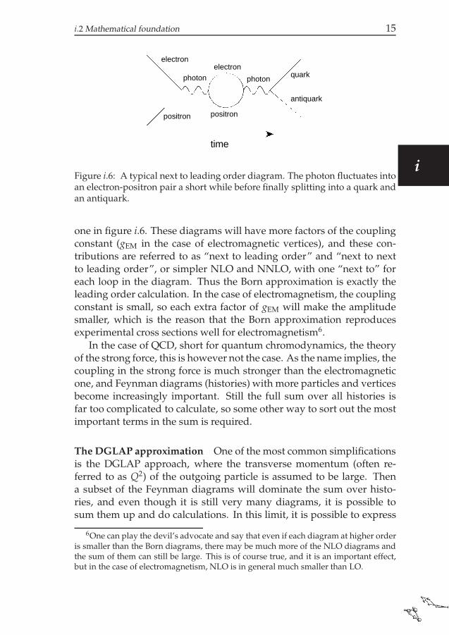
Figure i.6: A typical next to leading order diagram. The photon fluctuates intoan electron-positron pair a short while before finally splitting into a quark andan antiquark.
one in figure i.6. These diagrams will have more factors of the couplingconstant (gEM in the case of electromagnetic vertices), and these con-tributions are referred to as “next to leading order” and “next to nextto leading order”, or simpler NLO and NNLO, with one “next to” foreach loop in the diagram. Thus the Born approximation is exactly theleading order calculation. In the case of electromagnetism, the couplingconstant is small, so each extra factor of gEM will make the amplitudesmaller, which is the reason that the Born approximation reproducesexperimental cross sections well for electromagnetism6.
In the case of QCD, short for quantum chromodynamics, the theoryof the strong force, this is however not the case. As the name implies, thecoupling in the strong force is much stronger than the electromagneticone, and Feynman diagrams (histories) with more particles and verticesbecome increasingly important. Still the full sum over all histories isfar too complicated to calculate, so some other way to sort out the mostimportant terms in the sum is required.
The DGLAP approximation One of the most common simplificationsis the DGLAP approach, where the transverse momentum (often re-ferred to as Q2) of the outgoing particle is assumed to be large. Thena subset of the Feynman diagrams will dominate the sum over histo-ries, and even though it is still very many diagrams, it is possible tosum them up and do calculations. In this limit, it is possible to express
6One can play the devil’s advocate and say that even if each diagram at higher orderis smaller than the Born diagrams, there may be much more of the NLO diagrams andthe sum of them can still be large. This is of course true, and it is an important effect,but in the case of electromagnetism, NLO is in general much smaller than LO.
i

16 Introduction
the probability to find a gluon or a quark (or a parton as common name)with a given energy fraction x of the proton, and a given transverse mo-mentum Q2:
∂q(x, Q2)
∂ ln Q2=
αs
2π
∫ 1
x
dy
yP(x/y)q(y, Q2)
q is the distribution of partons and P is the splitting function in thissomewhat simplified version of the DGLAP equation. This formalismdescribes how the partons in a proton splits up, until finally one partoninteracts with a parton from the colliding particle and bounces out atan angle respective to the incoming direction. The DGLAP approxima-tion is valid as long as this last interaction is violent enough, that is ifthe outgoing particles have a large sideways (transverse) energy withrespect to the incoming direction.
Most of the new physics that for example LHC is looking for involvesvery violent collisions, and the DGLAP formalism can in general de-scribe these collisions. However, these collisions where new physicsis expected to show up are very rare. Almost every collision involvescomparably low transverse energies and the DGLAP approximation ispushed to its limit.
i.2.4 BFKL: a high energy approximation
There is another common approach known as the BFKL equation. Inthis case the partons are assumed to carry only a small fraction of theincoming particles energy. This approximation is increasingly valid asthe collision energy of particles increase, as the protons will tend to splitup in more particles, each carrying a smaller fraction of the total energy.So at LHC BFKL is expected to better describe collisions than at previ-ous, lower energy, colliders.
The BFKL equation is mathematically more complicated than theDGLAP equation though and significantly harder to use for predictions.As in the DGLAP formalism, the BFKL approximation selects a subsetof all the possible histories, and calculates and sums only those ampli-tudes. These amplitudes are referred to as the “leading logarithm” (or just “LL” for short) amplitudes, as they contain the largest power ofln(1/x). x is here the fraction of the protons energy that the collidingparton carries, and in the BFKL approximation, this is a small number(hence also referred to as “low x”). With x small, ln(1/x) will be large,which motivates that only the “leading logarithm” amplitudes are con-sidered.

i.3 The Lund Dipole Model: my contribution 17
There are however some technical problems. One is that the chosenLL amplitudes are actually not as dominating as one would like. In fact,if not only the LL diagrams are included, but also the amplitudes at thenext highest power in ln(1/x), “next to leading logarithm” (NLL), thecross sections can change significantly.
BFKL has mainly been used to determine the probability that a col-lision will happen at all (so called “inclusive” observables), rather thanto calculate exactly what all the outgoing particles will be (“exclusive”observables). Some approaches have been made to calculate these finalstates, but with very limited results.
During my PhD studies, I and my supervisors have been working ona formulation of the BFKL equation with colour dipoles that describeshow the incoming hadronic particles evolve. While it originally wasused only for inclusive observables, it is now developed to describefully exclusive final states. It is implemented in a computer simula-tor called DIPSY than can generate collisions between particles such asprotons, photons or heavy ions.
i.3 The Lund Dipole Model: my contribution
This section will present the work done during my time in Lund, and Iwill from here on assume that the reader has previous experience fromparticle physics phenomenology.
I have continued the work on the dipole model in transverse coor-dinate space developed by Emil Avsar with Leif Lonnblad and GostaGustafson [1–3], and developed it further. Some studies were done oninclusive and semi-inclusive observables in deep inelastic scattering inpaper I, on fluctuations in the interaction probability in paper II, and onthe correlations between subcollisions in paper III, but the majority ofthe effort has been put into providing fully exclusive final states, and im-plementing an event generator with final state radiation and hadroniza-tion from ARIADNE [4] and PYTHIA 8 [5–8].
I will first describe the model as it is in the current implementationof the event generator, but bear in mind that the first three publicationused an earlier version based on Avsar’s implementation. As this in-formation is already in paper IV, this will be a shorter summary to geta good picture without having to read through all the details. Furtherdetails can be found in the paper.
After that will follow a discussion about future applications in dif-ferent reaction, and what parts of the model can be further improved.
i
18 Introduction
i.3.1 Our model
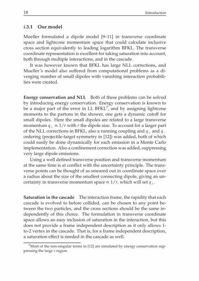
Mueller formulated a dipole model [9–11] in transverse coordinatespace and lightcone momentum space that could calculate inclusivecross section equivalently to leading logarithm BFKL. The transversecoordinate representation is excellent for taking saturation into account,both through multiple interactions, and in the cascade.
It was however known that BFKL has large NLL corrections, andMueller’s model also suffered from computational problems as a di-verging number of small dipoles with vanishing interaction probabili-ties were created.
Energy conservation and NLL Both of these problems can be solvedby introducing energy conservation. Energy conservation is known tobe a major part of the error in LL BFKL7, and by assigning lightconemomenta to the partons in the shower, one gets a dynamic cutoff forsmall dipoles. Here the small dipoles are related to a large transversemomentum q⊥ ∝ 1/r with r the dipole size. To account for a larger partof the NLL corrections in BFKL, also a running coupling and q+ and q−ordering (projectile-target symmetry in [12]) was added, both of whichcould easily be done dynamically for each emission in a Monte Carloimplementation. Also a confinement correction was added, suppressingvery large dipole emissions.
Using a well defined transverse position and transverse momentumat the same time is at conflict with the uncertainty principle. The trans-verse points can be thought of as smeared out in coordinate space overa radius about the size of the smallest connecting dipole, giving an un-certainty in transverse momentum space ∝ 1/r, which will set q⊥.
Saturation in the cascade The interaction frame, the rapidity that eachcascade is evolved to before collided, can be chosen to any point be-tween the two particles, and the cross sections should be the same in-dependently of this choice. The formulation in transverse coordinatespace allows an easy inclusion of saturation in the interaction, but thisdoes not provide a frame independent description as it only allows 1-to-2 vertex in the cascade. That is, for a frame independent description,a saturation effect is needed in the cascade as well.
7Most of the non-singular terms in [12] are simulated by energy conservation sup-pressing the large z region.

i.3 The Lund Dipole Model: my contribution 19
This triggered the inclusion of the dipole swing, a 2-to-2 interactionin the cascade that “swings” two dipoles by replacing them with twoother dipoles connecting the colour charge of one dipole with the anit-charge of the other dipole. The amplitude for the swing tends to replacelarge dipoles with small dipoles. Each dipole is randomly assigned acolour index, and only dipoles of the same colour are allowed to swing,to account for colour suppression in saturation. The swing can be inter-preted as an exchange of soft gluons, or as a quadrupole effect. It wasseen that the inclusive observables model got almost frame independentwith this addition. It also turned out to dampen the energy growth ofthe pp cross sections to a level that agreed with data.
In general the Monte Carlo turned out to accurately describe a widerange of observables:
• Total and elastic pp cross section as function of√
s.
• Elastic pp cross section as function of t.
• Diffractive excitation in pp as function of M2X.
• Total and elastic (DVCS) cross section in γ∗p as function of W andQ2.
• Elastic cross section in γ∗p as function of t.
• γ∗p → ρp (and other vector mesons) as function of W, Q2 and t.
This was done with only four tunable parameters: ΛQCD, the proton sizerp, the fluctuation in proton size ∆rp and the confinement scale rmax,also used for αS(r) freezeout. Notice that all four of these parametersare restricted (although ∆rp a bit less), in the sense that these quantitiesare to some extent known from experiments.
Final states Seeing the predictability for inclusive observables, we em-barked on the project to extend the model to completely exclusive finalstates. The first observation is that the non-diffractive cross section canbe rewritten in terms of independent subcollisions, so that it can be de-termined event-by-event which dipoles in the virtual cascade actuallyinteract. Then, by tracing them back through the evolution, it is pos-sible to divide up the partons in real partons that go to the final stateand virtual partons that are reabsorbed. These gluons are the q+ andq− ordered “backbone gluons”, that determine the inclusive cross sec-tion, and the remaining phase space for lower transverse momenta willbe covered by final state radiation by the Linked Dipole Chain modelbased on the CCFM formalism. As the colour flow is considered allthe way through this process it is natural to hadronize using the string
i

20 Introduction
fragmentation model.
Corrections needed: reweighting It is however not as straightfor-ward as it may sound in the paragraph above. One of the biggest prob-lems is that, since Mueller’s original model was designed for inclusivevariables, the weights for small non-interacting dipoles will sometimesbe overestimated. This does not affect any previous results, as non-interacting dipole do not affect the inclusive cross section, but it willgive a too strong tail to large q⊥ in the final state. This is compensatedfor by removing some of the real gluons corresponding to this overesti-mate, and the weights of the gluon chains are restored.
Ordering in the virtual cascade As the kinematics of the real gluonsare not known until the virtual gluons are reabsorbed, it is impossibleto know what phase space should be allowed for real emissions dur-ing the virtual cascade. This problem is extended by the fact that someof the real gluons will be removed in the reweighting in the previousparagraph. To solve this, an overestimate of the allowed phase space isused during the virtual cascade. However, a balance has to be found,as too large overestimate will overproduce virtual dipoles, and the in-teraction probability will be inflated. Much care has been taken to findan allowed phase space that covers most of the important final states,while still not inflating the inclusive observables.
Self consistency constraint: frame independence The above prob-lems get increasingly involved to handle in a saturated environment,where a gluon chain can split or merge at any point. Thus it has beenvery hard to use perturbative QCD to directly solve these issues. One ofthe most important tools has been the frame independence, that is thatevery observable should be the same no matter where the interactionframe is placed. It should not matter if the interaction frame is placed inthe detector frame or in the rest frame of one of the incoming particles,all observables should still give the same result.
This symmetry is not exactly manifested in this model at fixed order,as the corrections to the LL formulation are not cover in exactly equiv-alent ways in the cascade and in the interaction. Thus, the cross sectionwill differ depending on which part of the gluon chain is handled as theinteraction, and which part as a cascade.
So when perturbative QCD cannot provide a clear solution to theseproblems, we have let this full-order symmetry guide the choices.
i.3 The Lund Dipole Model: my contribution 21
Tuning Now that the model is extended to exclusive observables, anumber of new undetermined parameters and choices have been in-troduces. Every choice and parameter can not be fixed by theoreticalconsiderations and frame independence alone; some has to be tuned toexperimental data. We have started by tuning to inclusive observables:total and elastic pp and total γ∗p, before looking at exclusive observ-ables. As it turned out, many of the parameters and choices could beset from the frame independence and inclusive data, leaving only littlefreedom to tune to exclusive observables. As many of the degrees offreedom are heavily correlated, basically only the charged particle mul-tiplicity could be affected much. Once that was tuned to data, it washard to move other observables much without destroying inclusive ob-servables or frame independence.
It should be kept in mind that the tuning has been done by hand,and the data set that has been compared to is enormous: a big set of in-clusive data for pp and γ∗p, and all minimum bias data avaliable fromfor example CDF, ALICE and ATLAS. And further, each one of these ob-servables is required to be frame independent. With a more systematicapproach to tuning, the result can probably be significantly better.
i.3.2 Further applications
The exclusive observables presented in the last paper has been frompp only, but there is in principle nothing that stops us from collidingany hadronic particle and generate final states. There is implementedsupport for virtual photons and heavy ions, but it has not been tuned orcompared to data.
AA Maybe the most interesting reaction would be heavy ion colli-sions. With the dipole swing, there is a very detailed interaction be-tween partons in the initial state, both within and between the nucle-ons. There are currently no collective effects in the final state evolution,so DIPSY would probably not reproduce data in its present state, but itcan provide transverse position and momentum for every parton justafter collision, giving all the necessary initial conditions for any finalstate models, be it jet quenching on a parton level, or hydrodynamics.Here it should be mentioned that DIPSY describes all the fluctuationsin the initial state evolution, and could be used for observables such astriangular flow which are based on event-by-event fluctuations that areoften neglected in heavy ion observables.
i

22 Introduction
v2 in pp from elliptic flow As example of how the real gluons justafter the interaction can be used as input for collective effects, it has beenused to measure elliptic flow in pp at the LHC. This work has been donein collaboration with Emil Avsar, Yoshitaka Hatta, Jean-Yves Ollitraultand Takahiro Ueda. The transverse configureation of the real gluons areused to calculate the participant eccentricity and the density of the state.An empirical formula from hydrodynamics is used to calculate v2 fromthe transverse t = 0 configuration on an event-by-event basis. This isan example of where DIPSY shines, as we get the full fluctuations in thetransverse shape and density from the BFKL dynamics.
This is then compared to the v2 obtained from the event generatorwith the default treatment of the final state with final state radiation andhadronization as normal. These two can be compared, and are showingthe cases of no collective effects in the final state, and completely hydro-dynamical collective behaviour. As one goes to higher multiplicities,one expects the collective effects to be more important, and a possiblesignal for collective effects could be in v2 deviating from the defaultDIPSY towards the hydrodynamical result.
This work can be found in a preprint [13] based on a preliminaryversion of DIPSY, but is not included in the thesis as there is a technicalproblem with the v2 observable in default DIPSY. This problem is relatedto the pointlike valence partons in section i.3.3, and the balancing jet willtoo often end up outside of the detector range, giving a too small v2. Atthe time of printing, this problem is yet not solved, but we hope to soonhave improvements to present.
pA, γ∗A While AA is expected to have significant collective effects inthe final state evolution, pA and especially γ∗A will have much less,and DIPSY can be directly used to describe both inclusive and exclusiveobservables.
γ∗ p This reaction was well tested for inclusive observables, anddipole models are traditionally successful in describing DIS. It is a some-what different situation, as the valence partons of the photon will startthe evolution with a large q⊥, while the proton will start with a muchlower q⊥. This asymmetric evolution between a large and a small trans-verse momentum scale may highlight effects that were previously neg-ligible and thus allow for further tuning of the model. So with the pos-sible exception of a few corrections, we expect DIPSY to be able to re-produce exclusive γ∗p data as well.

i.3 The Lund Dipole Model: my contribution 23
i.3.3 Future development
The recent publication of the final state Monte Carlo does not providea final answer to how to get exclusive observables out of this dipolemodel. In fact, there is ample space for development, and I expect thatmore work in this model can significantly improve agreement with ex-periment. Here follows a list of areas where further attention could beuseful.
Real gluon ordering We are allowing real gluon chains ordered in q+
and q−, to approximately account for NLL BFKL and to match final stateradiation phase space, but as observables are very sensitive to this, fur-ther investigations should be made.
Ordering in the virtual cascade Ideally we want to keep the orderingin the cascade open enough so that every conceivable ordered real gluonchain always is considered, no matter which partons are reabsorbed.However, as the real chain is not known during the virtual cascade, thiswould mean a large overestimate of emissions, and the inclusive crosssections would be inflated. It is possible to make a compromise thatcan describe inclusive cross section without affecting the final state toomuch (in fact DIPSY does this), but more systematic work has to be doneon this problem.
Full NLL splitting functions in momentum space The interactionprobability was recalculated in momentum space for the exclusive ob-servables, as the coordinate space version had a logarithmic divergencefor small distances. As the momentum space splitting function in thecascade had no such serious flaws, it never got recalculated in momen-tum space. However, it could still improve the description of the finalstates. At that point, a closer comparison to the NLL splitting functioncould be made.
Pointlike valence partons A proton at the LHC comes in with an p+
of 7 TeV, and this energy is split up on the three valence partons in ourmodel. Some of this will radiate away during the cascade, but mostof it will remain in the valence parton, which means that there will bethree partons with a very large q+ still when the cascades has evolvedalmost all the way to the interaction frame. This will allow emissionswith very large q⊥ from three partons in almost every collision. Even
i

24 Introduction
though the large q⊥ is properly weighted with d2q⊥/q4⊥, one expects
a further suppression from the small energy fractions of most of theincoming parton.
The cause of the problem is that modeling the proton as three point-like partons is not realistic, so to remedy this issue, a natural approachwould be to smear out the valence partons in transverse space. Thiswould disallow hard emissions, as the small wavelength would onlyresolve a small part of the valence parton, effectively being the oppositeeffect of coherence. Work is currently ongoing on this problem, and wehope to soon have new results.
i.4 Introduction to papers
i.4.1 Paper I: Elastic and quasi-elastic pp and γ⋆p scattering inthe Dipole Model
In this paper the model for inclusive observables developed previouslyis compared to a large set of observables in both pp and γ∗p. The totaland elastic pp cross section had been described previously as functionof
√s, but now the elastic cross section as function of t is introduced,
and the fluctuations in the proton wavefunctions has to be strongly re-duced for the model to fit data. With this extra parameter introduced(bringing the total number of parameters up to 4), all pp data can beexplained by the model. Some predictive power is also seen, as the en-ergy dependence is to large extent independent of tuning but still agreeswith data.
To better describe γ∗p at low Q2, some soft correction are made tothe photon wavefunction, and to describe semi-inclusive γ∗p → ρp, adipole wavefunction is needed to describe the vector meson. The softcorrections introduce model dependence at low Q2 which is tuned toσtot(γ∗p) data, and two meson wavefunctions are used for comparison.
A large set of experimental data from HERA is compared to, and themodel is in agreement with data for all observables, even for very lowQ2. The good agreement with experiments from very few parameters isvery encouraging, and encourages the step to exclusive observables.

i.4 Introduction to papers 25
i.4.2 Paper II: Fluctuations, Saturation, and Diffractive Excita-tion in High Energy Collisions
In this paper diffraction is studied, and it is shown how the fluctua-tions in interaction probability causes diffractive excitation. Saturationis proven to play an important role in limiting the fluctuations, and thusthe diffractive excitations, in pp, and saturation is suggested to explainwhy diffractive excitation in γ∗p is larger than expected compared to pp.The impact parameter profile for diffraction is shown to take the shapeof a ring that grows with energy. This analysis takes full advantage ofthe dynamic way in which the BFKL fluctuations are incorporated inthe model, and can provide deep understanding of diffraction in thisformalism.
Further, our dipole model in the Good–Walker formalism is com-pared to the triple–Regge formalism. Although saturation is an integralpart of most triple-Regge models, and our dipole model, the compar-ison is made at a completely unsaturated level to easier compare theformalisms. It turns out that our dipole model without saturation re-produces the powerlike energy dependence at the foundation of anytriple-Regge model. The energy dependence of our model for total,elastic and diffractive cross sections corresponds to pomeron trajectoriesand pomeron couplings, which are in the range spanned by traditionaltriple–Regge analyses. This makes a connection between our perturba-tive BFKL-based model and triple-Regge. Note however that the NLLcorrections and confinement was still present in the comparison: onlysaturation was taken out. Pure LL BFKL may not be as similar to thetriple–Regge formalism.
This paper triggers the question if final states for diffractive excita-tion are possible to simulate. It turns out that the situation is signifi-cantly more complicated, as the cross section does not split into dipole-dipole interaction probabilities as neatly as in the non-diffractive case.Nonetheless, we hope to return to this problem.
i.4.3 Paper III: Correlations in double parton distributions atsmall x
In this paper we study correlations between two hard scatterings in app collision. It is done by collding a proton with two small dipoles rep-resenting the two hard interactions. The dependence on x1, x2, Q2
1, Q22
and distance b between the interactions are studied, giving a full doubleparton distribution including all correlations. This again takes advan-
i

26 Introduction
tage of the model including all fluctuations in the initial state cascadedynamically from BFKL.
We observe a strong dependence on Q2 and a weaker dependence onx. The factorisation of the b dependence is broken as hotspots appear atlow x and large Q2, and the distribution falls of quicker for large b if Q2
is large.
Events where one collision is in midrapidity, and the other shifted toa rapidity y are also studied. It turns out that the depende on y is weakfor the correlations, but not because the individual parton distributionfunctions depend weakly on y, but because the product of the distribu-tion functions from the two sides have opposite y dependencies.
i.4.4 Paper IV: Inclusive and Exclusive observables fromdipoles in high energy collisions
This paper presents the work started several years earlier, to model fullyexclusive observables with the model, and to implement an event gen-erator. It turns out to be more involved than initially expected andthere are many non-leading corrections that are hard or impossible totreat with perturbative calculations, but that still affects observables.Nonetheless many options can be excluded as they give effects con-flicting with known calculations (most frequently the d2q⊥/q4
⊥ tail tolarge q⊥), and other corrections turn out to not be needed in tuning (forexample colour reconnections). Of the remaining uncertainties, manycan be fixed by demanding frame independence, i.e. a self-consistencyconstraint, and most of the rest can be fixed from inclusive observablesalready studied in previous publications. The last remaining choices aretuned to exclusive data.
The resulting Monte Carlo, DIPSY, while not as accurate as PYTHIA 88 tune 4C, is providing a competitive description of minimum bias andunderlying event data at the Tevatron and LHC. As it is conceptuallydifferent from the other event generators, it provides a good compari-son, and the dynamic description of the incoming virtual cascade pro-vides a unique opportunity for many studies, not least in heavy ionphysics.
i.4.5 List of contributions
• Paper I: Elastic and quasi-elastic pp and γ⋆p scattering in the
Dipole Model

i.5 A PhD defence for a non-physicist 27
I wrote the new computer code necessary and ran all the simula-tions. I also contributed to the theoretical work and wrote a smallpart of the paper.
• Paper II: Fluctuations, Saturation, and Diffractive Excitation in
High Energy Collisions
For this paper I again did all the simulations, contributed to thetheoretical work and wrote parts of the paper.
• Paper III: Correlations in double parton distributions at small x
I prepared the computer program for the new observables, but didnot run the simulations. I contributed to the theoretical work, butwrote only little of the paper.
• Paper IV: Inclusive and Exclusive observables from dipoles in
high energy collisions
This paper cover the bigger part of the thesis, and included rewrit-ing the entire computer program. While Leif Lonnblad organisedmost of the structure, I wrote almost all the code, and designedmany of the algorithms. I contributed to the theoretical work andwrote most of the paper.
i.5 A PhD defence for a non-physicist
This section is mainly aimed at those going to their first PhD defence inphysics, and some general information and advice is presented.
i.5.1 The schedule
The day begins with the defence at 10.15 (you probably want to be about5-10 minutes early so you can get a good seat8, and an extra 5 minutesif you want to get coffee or tea). At the defence, the opponent start witha short presentation about the general area at as low level as possible,and will then hand over to me to shortly present my work which will bemore technical. This will be about 30-45 minutes in total, and after thatthe main session starts, where the opponent will ask me questions aboutmy work. After that, the 3 jury members will ask me a few questionseach as well and finally the audience is allowed to ask me questions.There is no formal time limit, but usually the questions are done a bitafter 12.
8You will notice that the jury and supervisors in general sit in the front rows, whilemost of the rest of the staff (specially the other PhDs) sit in the very back.
i

28 Introduction
After the defence there will be mingling in the coffee room whilewaiting for the jury to make a decision that will be announced. Somesmall lunch is also served at this point. After lunch people go back towork for a few hours before preparing for the party at 19.
i.5.2 What to do during the defence?
First, if you know that you tend to fall asleep when bored, make sureto get coffee before the defence! Ask someone that looks like a physicistfor directions on where to get it.
Once at the defence, the presentation by the opponent will probablybe the easiest to follow, so try to stay awake at least that part. After that,it will be increasingly hard to follow the details. However, the defencecan still be enjoyed even without understanding every single subtlety.Some examples:
• One can often understand if a question was tricky or not from toneof voice, body language and how fast the reply is.
• If you would like to understand the physics a bit more, but can’tfollow the discussion, try reading the introduction above.
• Drinking game. Pick keywords such as “dipole”, “parton”, “inter-action”, “cascade”, “proton”, and drink every time your word ismentioned9.
• Hangman is great fun. Open a random page in the articles in thesecond half of the thesis, and pick a word that you have no ideawhat it means, and make a friend try to guess it. If you don’thave pen and paper, you can scribble in the blank pages at thestart/end of the thesis, and you can silently ask to borrow a penfrom someone else in the audience.
9No responsibility taken for caffeine overdose.

i.5 A PhD defence for a non-physicist 29
Acknowledgments
I am very lucky to have my two supervisors Leif Lonnblad and GostaGustafson, who have always been avaliable for me. Leif has shown mehow powerful computers can be for solving physics, and I have triedto absorb some of Gostas ability to formulate even the most complexargument in a short, yet convincingly clear, manner.
I want to thank Emil Avsar, Yoshitaka Hatta, Jean-Yves Ollitrault andTakahiro Ueda for inviting me to work with them, it has been a veryuseful experience. It has also been a pleasure to work with Andras Ster,I have always enjoyed your visits to Lund.
Apart from my supervisors, there are many others in Lund that havehelped me with my work. For example Richard Corke who gave mecomputer support when I was too embarrassed to ask Leif a third time.Torbjorn Sjostrand who always has time for a full explanation. PeterChristiansen who is always full of ideas, and a source for heavy ion ex-pertice. And not least Alejandro Alonso for helping me with the ATLASdata.
I am grateful for a big group of proof-readers: Torbjorn Sjostrand fortaking the time to read through and provide top-notch feedback on theintroduction and all the papers, making the end result so much better.Konrad Tywoniuk, Angela Pizzolla, Nils Lavesson and my family forreading and correcting this introduction.
The main reason I went into physics rather than mathematics to-wards the end of my undergraduate studies was that in physics peopleseemed more fun. The people here at theoretical physics in Lund, andour experiementalist friends, certianly delivered; it has been a lot of fun.You are too many to list here, but a special mention has to go the groupof seven from the Lund-HEP EST graduate school that helped me somuch in feeling at home from the first day. Thanks to everyone for thecompany, see you around and stay sharp. ;)
Last, I want to thank Angela for company and support. Now let’s gosomewhere warmer.
i

30 Introduction
i References
[1] E. Avsar, G. Gustafson, and L. Lonnblad, “Energy conservationand saturation in small-x evolution,” JHEP 07 (2005) 062,arXiv:hep-ph/0503181.
[2] E. Avsar, G. Gustafson, and L. Lonnblad, “Small-x dipoleevolution beyond the large-N(c) limit,” JHEP 01 (2007) 012,arXiv:hep-ph/0610157.
[3] E. Avsar, G. Gustafson, and L. Lonnblad, “Difractive Excitation inDIS and pp Collisions,” JHEP 12 (2007) 012, arXiv:0709.1368[hep-ph].
[4] L. Lonnblad, “ARIADNE version 4: A Program for simulation ofQCD cascades implementing the color dipole model,”Comput. Phys. Commun. 71 (1992) 15–31.
[5] B. Andersson, G. Gustafson, and B. Soderberg, “A GENERALMODEL FOR JET FRAGMENTATION,” Z. Phys. C20 (1983) 317.
[6] B. Andersson, G. Gustafson, G. Ingelman, and T. Sjostrand,“Parton fragmentation and string dyanmics,” Phys. Rept. 97 (1983)31.
[7] T. Sjostrand, S. Mrenna, and P. Z. Skands, “A Brief Introduction toPYTHIA 8.1,” Comput. Phys. Commun. 178 (2008) 852–867,arXiv:0710.3820 [hep-ph].
[8] T. Sjostrand, S. Mrenna, and P. Z. Skands, “PYTHIA 6.4 Physicsand Manual,” JHEP 05 (2006) 026, arXiv:hep-ph/0603175.
[9] A. H. Mueller, “Soft gluons in the infinite momentum wavefunction and the BFKL pomeron,” Nucl. Phys. B415 (1994) 373–385.
[10] A. H. Mueller and B. Patel, “Single and double BFKL pomeronexchange and a dipole picture of high-energy hard processes,”Nucl. Phys. B425 (1994) 471–488, hep-ph/9403256.
[11] A. H. Mueller, “Unitarity and the BFKL pomeron,” Nucl. Phys.B437 (1995) 107–126, hep-ph/9408245.
[12] G. P. Salam, “An introduction to leading and next-to-leadingBFKL,” Acta Phys. Polon. B30 (1999) 3679–3705, hep-ph/9910492.
i References 31
[13] E. Avsar, C. Flensburg, Y. Hatta, J.-Y. Ollitrault, and T. Ueda,“Eccentricity and elliptic flow in proton-proton collisions fromparton evolution,” arXiv:1009.5643 [hep-ph].
i


I
Elastic and quasi-elastic pp and γ⋆p
scattering in the Dipole Model
Christoffer Flensburg, Gosta Gustafson and Leif Lonnblad
Department of Theoretical Physics, Lund University,Solvegatan 14A, SE–223 62 Lund, Sweden
European Physics Journal C60 (2009) 233-247 [hep-ph/0807.0325].
We have in earlier papers presented an extension of Mueller’s dipolecascade model, which includes sub-leading effects from energy conser-vation and running coupling as well as colour suppressed saturationeffects from pomeron loops via a “dipole swing”. The model was ap-plied to describe the total and diffractive cross sections in pp and γ∗pcollisions, and also the elastic cross section in pp scattering. In this paperwe extend the model to describe the corresponding quasi-elastic crosssections in γ∗p, namely the exclusive production of vector mesons anddeeply virtual compton scattering. Also for these reactions we find agood agrement with measured cross sections. In addition we obtain areasonable description of the t-dependence of the elastic pp and quasi-elastic γ⋆p cross sections.
With kind permission of The European Physics Journal (EPJ).
I

34 Elastic and quasi-elastic pp and γ⋆ p scattering in the Dipole Model
I.1 Introduction
We have in a series of papers [1–3] presented an extention of Mueller’sdipole cascade model [4–6] implemented in a Monte Carlo program,which includes sub-leading effects from energy conservation and run-ning coupling, as well as colour suppressed effects from pomeron loopsvia a dipole swing mechanism. It also includes a consistent treatmentof non-perturbative confinement effects, which suppress dipoles withlarge transverse extension.
The advantage of a cascade model formulated in transverse coordi-nate space is the possibility to include effects of multiple collisions andsaturation in a straight forward way. While analytic results have mainlybeen presented for the asymptotic behavior of total and diffractive crosssections, Monte Carlo simulations facilitate studies of non-leading ef-fects and more quantitative results. A simulation of Mueller’s initialmodel was presented by Salam in ref. [7]. Although giving finite re-sults for the total cross section, this leading log evolution suffers fromdivergences for small dipoles, which caused numerical problems withvery large gluon multiplicities and prevented simulations at higher en-ergies. One important result from this analysis was the very large fluc-tuations in the evolution [8]. As the ratio between the elastic and thetotal cross sections is determined by the fluctuations in the scatteringprocess, this implies that less fluctuations is needed in the impact pa-rameter dependence, to reproduce the experimental data. As a resultwe found in ref. [3] that including the fluctuations in the evolution im-plies that the impact parameter profile is not as “black and white” as inanalyses where only fluctuations in the impact parameter are taken intoaccount.
In the model described in refs. [1–3] we include a number of sub-leading effects, with the aim that we in the end will be able to describenot only the total and diffractive cross sections, but also to generate fullyexclusive final states. The main ingredient in our model is energy con-servation, which is included by assigning a transverse momentum toeach emitted gluon given by the maximum inverse size of the neighbor-ing dipoles. As a result this also implies that the singularities for smalldipoles are avoided. Other features are saturation effects in the evolu-tion through a dipole swing mechanism, and a consistent treatment ofconfinement and running coupling effects in both dipole emissions anddipole–dipole interactions.
Taken together with a very simple model for the initial proton wave-
I.1 Introduction 35
function, these features allow us to obtain a Lorentz-frame indepen-dent description of total cross sections, both for pp and DIS, using basi-cally only two free parameters, a confinement scale ρmax and ΛQCD [3].The model gives a good description of measurements of the total anddiffractive cross sections in pp and γ∗p collisions, and also for the elas-tic cross section in pp. In this paper we will continue our investiga-tions with an analysis of exclusive production of vector mesons andreal photons in γ∗p. The aim is to further test our model, and in par-ticular to study the effect of the fluctuations in the cascade. We alsoextend the analyses to include the t-dependence of the (quasi-)elasticcross sections, including also elastic pp scattering, which in particulargives information about the properties of the incoming proton state. Wehere include effects of scewedness in the photon wavefunction, but ar-gue that such effects in the proton wavefunction ought to be small atHERA and proton collider energies.
In the eikonal approximation the quasi-elastic γ∗p collisions con-tain three elements: the virtual photon–dipole vertex, the dipole–protonscattering amplitude, and the vertex for the transition between thedipole and the final vector meson or real photon. Here the first compo-nent can be calculated perturbatively, although a hadronic componentmust be included at lower Q2-values. In an extensive study Forshawet al. [9, 10] have analyzed the results obtained from a set of models forthe dipole–proton scattering and for the vector meson wavefunctions,and compared them with experimental data. In this paper we want tocarry out a similar analysis, but now use our dipole cascade model forthe dipole–proton scattering. We are here particularly interested in ef-fects of fluctuations in the cascade evolution, which are not included inthe analyses by Forshaw et al. We also want to use this study to putconstraints on the state of the incoming proton.
An approach to describe both pp and γ∗p collisions in a dipole for-malism has also been presented by Shoshi et al. [11]. One essential dif-ference is that in their approach the energy dependence is describedby a combination of a soft and a hard pomeron, with parameters fittedto data. In our model the energy dependence is fully determined bythe perturbative dipole cascade evolution. Naturally this dynamical de-scription limits the application of our model to relatively high energies.
We begin in section I.2 with discussing the eikonal formalism forexclusive vector meson production, whereafter we describe our modelfor dipole evolution and dipole–dipole scattering in section I.3 and themodels we use for the proton, photon and vector meson wavefunctions
I

36 Elastic and quasi-elastic pp and γ⋆ p scattering in the Dipole Model
in section I.4. In section I.5 we retune the parameters of our model todata on total and elastic pp cross sections and the total γ⋆p cross sec-tion before we present our results on quasi-elastic γ⋆p cross sections onsection I.6. Finally we present our conclusions in section I.7
I.2 Formalism
I.2.1 The dipole cascade model and the eikonal approximation
As discussed in the introduction, our model for pp collisions and DIS isan extension of Mueller’s dipole cascade model [4–6]. In this formalismthe probability per unit rapidity Y that a dipole (x, y) emits a gluon attransverse position z is given by
dPdY
=α
2πd2z
(x − y)2
(x − z)2(z − y)2, with α =
3αs
π. (I.1)
The evolution of this cascade agrees with the leading order BFKL evo-lution. As a consequence, the total number of dipoles grows exponen-tially. This also implies a strong growth for the total cross section which,however, is tamed by taking multiple dipole interactions into account.The scattering probability between two elementary colour dipoles withcoordinates (xi, yi) and (xj, yj) respectively, is given by
fij = f (xi, yi|xj, yj)
=α2
s
8
[
log
( (xi − yj)2(yi − xj)
2
(xi − xj)2(yi − yj)2
)]2
. (I.2)
Within this eikonal formalism the transverse coordinates are notchanged under the emission or scattering processes in eqs. (I.1) and(I.2). Therefore unitarity constraints and multiple scattering are easilyaccounted for by the exponentiated expression
T(b) = 1 − e− ∑ fij ≡ 1 − e−F, (I.3)
which implies that the scattering probability never exceeds 1. We notethat the splitting probability in eq. (I.1) is singular for small dipole sizesx − z or z − y, but these small dipoles have a small probability to inter-act with the target, and the eikonal F = ∑ fij is finite.
In the model developed in refs. [1–3], we extended Mueller’s cascademodel to include sub-leading effects from energy conservation and a

I.2 Formalism 37
running coupling, saturation effects not only in the dipole–dipole sub-collisions but also within the individual cascades, and effects of confine-ment. These features are further discussed in sec. I.3.
The model is supplemented by a non-perturbative model for an ini-tial proton in terms of three dipoles. In the eikonal approximation thetotal and the diffractive (including the elastic) cross sections are thengiven by
σtot = 2∫
d2b 〈(1 − e−F)〉,
σdiff =∫
d2b 〈(1 − e−F)2〉. (I.4)
The diffractive cross section can be separated in elastic scattering anddiffractive excitation:
σel =∫
d2b (〈1 − e−F〉)2,
σdiff exc =∫
d2b{
〈(1 − e−F)2〉 − (〈1 − e−F〉)2}
. (I.5)
Thus the separation between elastic and inelastic diffraction is deter-mined by the fluctuations in the scattering amplitude. The average ineqs. (I.4) and (I.5) is taken over the different incoming dipole configu-rations and different cascade evolutions, which thus give two separatesources for fluctuations.
I.2.2 DVCS and exclusive vector meson production in γ∗p col-lisions
We want to study the exclusive processes
γ∗ p → V p, V = γ, ρ, ψ, . . . (I.6)
In the dipole model the virtual photon is split into a qq pair long beforethe collision. This dipole scatters elastically against the proton, and afterthe scattering the pair joins again forming a real photon or a vector me-son. The formulation in the transverse coordinate plane makes it easierto study these pseudo-elastic reactions, and in the eikonal approxima-tion the scattering amplitude is expressed in terms of three components:
ℑAλ(s, b) = s ∑f ,h,h
∫ ∫
dz d2r Ψ∗Vλf hh
(r, z) Ψγλ
f hh(r, z, Q2)
× σdp(s, r, b, z). (I.7)
I

38 Elastic and quasi-elastic pp and γ⋆ p scattering in the Dipole Model
Here r is the transverse size of the dipole, z and 1− z the fractions of thephoton or vector meson carried by the quark and antiquark respectively,and h and h their helicities. λ denotes the photon or vector meson he-licity, σdp is the dipole–proton scattering probability with b the impactparameter, and s the total energy squared.
Neglecting the small contribution from the real part of the ampli-tude, the total cross section is given by
σλ(γ∗p → Vp) =1
4s2
∫
d2b |Aλ(s, b)|2. (I.8)
I.2.3 Differential cross sections
For scattering of a point particle the differential cross section dσel/dtis obtained from the Fourier transform of the scattering amplitude ineq. (I.3):
dσλ
dt=
1
4π
∣
∣
∣
∣
∫
d2b eiqb〈1 − e−F〉∣
∣
∣
∣
2
, (I.9)
with t = −q2. For a qq dipole described by an extended wavefunctionΨ(r, z), Bartels, Golec-Biernat and Peters [12] have shown that the effectof non-forward amplitudes (also referred to as scewedness) are prop-erly taken into account by replacing the exponential eiqb by eiq(b−(1−z)r).Thus we obtain the following expression for the differential cross sec-tions:
dσλ
dt=
1
16π
∣
∣
∣
∣
∑f ,h,h
∫ ∫ ∫
dz d2r d2b eiq(b−(1−z)r)
× Ψ∗Vλf hh
(r, z) Ψγλ
f hh(r, z, Q2)
× σdp(s, r, b, z)
∣
∣
∣
∣
2
. (I.10)
The effect of including the factor e−i(1−z)qr is small for large Q2,where the width of the r-distribution ∼ 1/
√
z(1 − z)Q2 is small com-pared to the extension of the proton target, which in our model is de-termined by the parameter Rp estimated to be around 3 GeV−1. As anexample we find in section I.6 (figure I.7) that for DVCS the slope of thet-distribution at Q2 = 8 GeV2 is increased by about 7%. The effect iscorrespondingly reduced (increased) for higher (lower) Q2.
Naturally a similar scewedness effect should come from the dipoleswithin the proton. This is more difficult to estimate, but the effect should

I.3 The improved dipole cascade 39
also here be determined by the ratio ((1 − z)rdipole/Rp)2. In our simula-tions of pp collisions at the Tevatron (W=2 TeV) we find a typical valuefor those dipoles which do interact in the collision is about 1/(1.5GeV). (Thetypical size is here estimated from the median of the distribution.) Thuswe estimate the effect from scewedness in the proton wave function tobe of the order ((1− z)rtypical/Rp)2 ∼ 0.01, if typical z-values are around0.5. A similar estimate can also be obtained from fits to minimum biasand underlying events in pp scattering. As an example, the PYTHIA 8event generator [13] gives a good description of the underlying eventsat the Tevatron if a cutoff of around 2 GeV is introduced to regularizethe (mini-)jet cross section, which diverges like dp2
⊥/p4⊥ in collinear fac-
torization. This cutoff value can be interpreted as a screening lengthwhich in turn can be related to a typical dipole size.
It would be valuable to study this effect in more detail to find a betterquantitative estimate. However, in view of the small value of the roughestimates above, we will in the present analysis neglect the effects ofscewedness in the proton wave function. We note that in the rest frameof a 2 TeV pp-collision, the energy corresponds to an evolution over 7units of rapidity for each of the protons. This corresponds to the protonevolution in DIS at W ≈ 100 GeV, and the estimate above is thereforealso relevant for the proton wavefunction in DIS at HERA energies.
I.3 The improved dipole cascade
As discussed in the introduction, the model developed in refs. [1–3]. isan extension of Mueller’s dipole cascade model, which includes sub-leading effects from energy conservation and a running coupling, satu-ration effects not only in the dipole–dipole subcollisions but also withinthe individual cascades, and effects of confinement. As mentionedabove, an essential point is here that we include the effect of fluctuationsin the dipole cascades in the calculation of the elastic or quasi-elasticcross sections.
I.3.1 Non-leading perturbative effects
Energy-momentum conservation
It is known that the large NLO corrections to the BFKL evolution arereduced significantly if proper energy conservation is included in theleading order. In our model a small transverse extension is interpreted
I

40 Elastic and quasi-elastic pp and γ⋆ p scattering in the Dipole Model
as a large transverse momentum. This interpretation is supported by theresulting analogies between the dipole chains in coordinate space andthe chains in the LDC model, which is formulated in momentum spaceand interpolates smoothly between DGLAP and BFKL evolution. Tak-ing energy-momentum conservation into account is most easily donein a Monte Carlo (MC) simulation. Conserving both light-cone compo-nents, p+ and p−, implies that we also satisfy the so called consistencyconstraint [14]. As small dipoles in our formalism correspond to largetransverse momenta, energy conservation also gives a dynamical cutofffor the otherwise diverging number of small dipoles, and thus makesthe MC simulation much more efficient.
Running coupling
In our simulations we also include non-leading effects from the runningof αs, both in the dipole splitting and in the dipole–dipole scatteringprobability. In the dipole emissions the scale in the coupling is given bymin(r, r1, r2), where r is the size of the mother dipole which splits into r1
and r2. This is the most natural choice and is also consistent with recentNLO calculations [15–17]. For the dipole–dipole scattering the situationis somewhat more complicated with basically six different dipole sizesinvolved. We have chosen to use the scale min(|xi − yi|, |xj − yj|, |xi −yj|, |yi − xj|). In order to avoid divergencies the coupling is in all cases
frozen so that αs(r) → αs(min(r, rmax)), where rmax is the confining scalediscussed in section I.3.3 below.
I.3.2 Saturation within the cascades
Mueller’s cascade includes saturation effects from multiple collisionsin the Lorentz frame chosen for the calculation, but not saturation ef-fects from gluon interaction within the individual cascades. The resultis therefore dependent on the chosen Lorentz frame. In ref. [2] we im-proved our model by allowing (colour suppressed) recouplings of thedipole chain during the evolution, a “dipole swing”. The swing is a pro-cess in which two dipoles (xi, yi) and (xj, yj) are replaced by two new
dipoles (xi, yj) and (xj, yi). The process can be interpreted in two ways.
There is a probability 1/N2c that the two dipoles may have the same
colour, and the quark at xi and the antiquark at yj form a colour sin-glet. In this case the best approximation of the quadrupole field oughtto be obtained by the closest charge-anticharge combinations. Here the

I.3 The improved dipole cascade 41
swing is therefore naturally suppressed by 1/N2c , and it should be more
likely to replace two given dipoles with two smaller ones. Secondly, wemay see it as the result of a gluon exchange between the dipoles, whichresults in a change in the colour flow. In this case the swing would beproportional to α2
s , which again is formally suppressed by N2c , compared
to the splitting process in eq. (I.1), which is proportional to α = Ncαs/π.In the MC implementation each dipole is randomly given one of N2
c
possible colour indices. Only dipoles with the same colour can swing,and the weight for a swing (x1, y1), (x2, y2) → (x1, y2), (x2, y1) is deter-mined by a factor proportional to
(x1 − y1)2(x2 − y2)
2
(x1 − y2)2(x2 − y1)
2. (I.11)
This implies that the swing favors the formation of smaller dipoles.The number of dipoles is not reduced by the swing, but the fact thatsmaller dipoles have smaller cross sections gives the desired suppres-sion of the total cross section. Although not explicitely frame indepen-dent the results from the MC simulations are very nearly independentof the Lorentz frame used for the calculations.
I.3.3 Confinement effects
Mueller’s dipole model is a purely perturbative process. It should there-fore be applied to small dipoles, e.g. to heavy quarkonium states. Whenapplying the dipole formalism to collisions with protons it is necessaryto take confinement into account, in order to prevent the formation ofvery large dipoles. Confinement effects must also suppress long rangeinteractions between colliding dipoles. In ref. [3] a consistent treatmentof confinement was presented by replacing the Coulomb potentials ineqs. (I.2) and (I.13) by screened potentials, with a screening length rmax.
Obviously the dipoles produced in the splitting process in eq. (I.1)cannot become too large, and it is natural to introduce a scale rmax, sothat larger dipoles are suppressed. In a similar way confinement mustsuppress long range interactions between colliding dipoles.
The formula for fij in eq. (I.2) is just the two dimensional Coulombpotential, and can be written as
f (xi, yi|xj, yj) =g4
8
[
∆(xi − xj) − ∆(xi − yj)
−∆(yi − xj) + ∆(yi − yj)
]2
(I.12)
I

42 Elastic and quasi-elastic pp and γ⋆ p scattering in the Dipole Model
where ∆(r) is the Green’s function given by
∆(r) =∫
d2k
(2π)2
eik·r
k2. (I.13)
To take confinement into account we replace the infinite range Coulombpotential with a screened Yukawa potential. This implies that theCoulomb propagator 1/k2 in eq. (I.13) is replaced by 1/(k2 + M2),where M = 1/rmax is the confinement scale. As a result, the four func-tions ∆ in eq. (I.12) will be replaced by
∫
d2k
(2π)2
eik·r
k2 + 1/r2max
=1
2πK0(r/rmax) (I.14)
with K0 a modified Bessel function. For small separations, where r ≪rmax, the function K0(r/rmax) behaves like ln(rmax/r), and we then rec-ognize the result in eq. (I.2). For large separations, r ≫ rmax, K0(r/rmax)
falls off exponentially ∼√
πrmaxr e−r/rmax , as expected from confinement.
In a similar way, the underlying Coulomb potential in the dipolesplitting function in eq. (I.1) can be replaced by a screened Yukawa po-tential, using again the replacement 1/k2 → 1/(k2 + 1/r2
max). The mod-ified splitting probability is then given by
dPdY
→ α
2πd2z
{
1
rmax
x − z
|x − z| K1
( |x − z|rmax
)
− 1
rmax
y − z
|y − z| K1
( |y − z|rmax
)}2
.
(I.15)
For small arguments K1(r/rmax) ≈ rmax/r, from which we get back theresult in eq. (I.1), while for large arguments K1(r/rmax) ∼
√πrmax/r ·
e−r/rmax , and once again we obtain an exponentially decaying field.
I.4 Initial wave functions
I.4.1 Proton wave function
In ref. [2] we also introduced a simple model for the proton in termsof three dipoles with extensions determined by a Gaussian distribution.The resulting model was in good agreement with total cross sections

I.4 Initial wave functions 43
for both DIS and pp collisions. It was shown in [18] that, although afull gluon cascade from three valence quarks in a proton is not a sim-ple expression, the emission of the first gluon has the same distributionin transverse space as three dipoles, only with half the intensity. Thus,by modeling the proton with a closed chain of three gluons we emulatethe fact that a proton at rest may contain more charges than its valencequarks. This is analogous to the finding of Gluck, Reya and Vogt, whoneeded a large valence-like gluon component when trying to fit par-ton densities evolved from a very low scale [19]. Thus, although not afully realistic description of the initial non-perturbative proton state, themodel appears to give a fair representation of the multi-dipole systemobtained at the low x-values, which are important for the high energycollisions.
The results turned out to be almost independent of the shape ofthe three starting gluons, except for the size of the triangle. In fact,equilateral triangles that were allowed to vary in only size and ori-entation turned out to model the proton as well as more complicatedformations. With a Gaussian distribution for the size of equilateraltriangles, motivated by the exponential dependence on t for the elas-tic cross section, data on total cross sections for DIS and pp collisionsare well reproduced, when the width of the Gaussian was tuned to3.5 GeV−1 ≈ 0.66 fm.
As discussed above, the differential and elastic cross sections are de-termined by the fluctuations in the scattering amplitude, and in ref. [3] itwas pointed out that a Gaussian wavefunction as discussed above mustoverestimate the fluctuations of the incoming state in its rest frame. Theprobability for the three quarks to simultaneously be located in a singlepoint ought to be suppressed, and it was emphasized that the expo-nential t-dependence of the elastic cross section, which motivated theGaussian shape, is only observed for |t| < 0.15 GeV2, corresponding tob >∼ 1 fm. A wavefunction of the form
|Ψ|2 = C e−(r−Rp)2/w2(I.16)
was also tested, and found to give essentially identical total cross sec-tions. The fluctuations are here suppressed by a small value of w, andin ref. [3] it was observed that reducing the fluctuations to a minimumgave good agreement with the integrated elastic and diffractive crosssections in pp collisions. Lacking further constraints we could, how-ever, only present an upper limit for σel, by neglecting the fluctuationsin the wavefunction, thus including only those in the cascade evolution.
I

44 Elastic and quasi-elastic pp and γ⋆ p scattering in the Dipole Model
An essential motivation for the present analysis of quasi-elastic γ∗pcross sections and of the t-dependence of the pp elastic cross section, isto check whether the fluctuations in the dipole cascade model are alsoconsistent with these observables, and if more constraints can be put onthe shape of the initial proton state. In this analysis we will use the two-parameter form in eq. (I.16), and see if this can be adjusted to reproducealso the (quasi-)elastic cross sections.
At this point we also note that in many analyses the fluctuations inthe cascade evolution are neglected. This means that e−F is replacedby e−<F> in eqs. (I.4) and (I.5). Including also the fluctuations in thecascade implies that the impact parameter profile has to be more “gray”and less “black and white”. As an example the amplitude 〈T(b = 0)〉 isa factor 2/3 smaller in our formalism than in the analysis by Kowalskiand Teaney [20], for a dipole of size 2 GeV−1 and x = 10−4 − 10−5.
I.4.2 Photon wavefunction
Large Q2
For large Q2 the coupling of the γ∗ to the qq pair can be calculated per-turbatively. The well known result to leading order is
Ψγ0
f hh(Q, r, z) =
√αEMNC
πQz(1 − z)e f K0(rε f )δhh
Ψγ+f hh
(Q, r, z) =
√αEMNC/2
πe f
×(
ieiθ(
zδh+δh− − (1 − z)δh−δh+
)
ε f K1(rε f )
+δh+δh+m f K0(rε f ))
(I.17)
withε f =
√
z(1 − z)Q2 + m2f . (I.18)
Here λ = 0 and + denote the longitudinal and transverse wavefunc-tions respectively, f denotes the quark flavour, and K0 and K1 are modi-fied Bessel functions. e f is the electric charge of the quark in units of theproton charge and m f the effective mass of the quark.
Smaller Q2
For smaller Q2 the photon has also a hadronic component. In [21]it was shown that also the total γ⋆p cross section at HERA could be

I.4 Initial wave functions 45
well described over a wide range of energies and virtualities, when thehadronic component was simulated by a relatively small effective quarkmass ≈ 60 MeV. For the exclusive reactions studied here we need a morecareful treatment of the hadronic component, and we expect that theseprocesses can provide relevant constraints on the photon wavefunction.The hadronic component should be particularly important for the realphotons produced in Deeply virtual Compton scattering (DVCS).
For small Q2 a small effective quark mass allows for rather largedipoles with a corresponding large cross section. In the present anal-ysis we include an improved description of confinement effects in thedipole evolution (see section I.3.3), and we will therefore try to includeconfinement effects also in the photon wavefunction. Our photon modelis inspired by the Vector Meson Dominance modeling introduced byForshaw et al. in [9] (which, in turn, was inspired by [22]). This modelcontains an enhancement factor for dipoles of a typical hadronic size,together with a large quark mass which suppresses dipoles larger thanthe confinement scale. In our model we will use the same enhancementfactor, but we use a suppression of large dipoles related to the confine-ment scale ρmax , instead of the large quark mass used in ref. [9].
The actual implementation in our MC program relies on shrinkingdipoles larger than ρmax by reducing the size rpert generated accordingto the perturbative photon wavefunction to rsoft, defined by
rsoft(rpert) = Rshrink
√
√
√
√ln
(
1 +r2
pert
R2shrink
)
. (I.19)
For small dipoles this gives rsoft ≈ rpert, but for large dipoles it givesa Gaussian suppression. The parameter Rshrink is adjusted to give thesame effective cutoff, ρmax, as the one obtained for large dipoles in thecascade evolution. This is obtained for Rshrink = 4.3 GeV−1.
The enhancement factor for dipoles with a typical hadronic size, in-troduced in ref. [9], is given by the form
f (r) =1 + BV exp(−(r − RV)2/w2
V)
1 + BV exp(−R2V/w2
V)(I.20)
This factor multiplies the squared photon wavefunction after the shiftin eq. (I.19). The enhancement resembles very much the shape we usefor the proton wavefunction in eq. (I.16), and we can think of the thewhole correction
∣
∣Ψγ(rpert)∣
∣
2 → |Ψγ(rsoft)|2 f (rsoft) (I.21)
I

46 Elastic and quasi-elastic pp and γ⋆ p scattering in the Dipole Model
as the modeling of the virtual photon fluctuating into vector mesonstates with r-values of a hadronic scale. Partly this enhancement canbe thought of as due to a longer lifetime of these states, and partly asimulation of a gluonic component in the vector meson, in a way simi-lar to our model of the initial proton wavefunction in section I.4.1. Thephoton model contains three adjustable parameters, BV , RV , and wV ,which have to be determined from experiments.
I.4.3 Meson wavefunctions
The wavefunction of a vector meson cannot be calculated perturba-tively, and has to be described by models. In the rest frame it is gen-erally assumed that the lowest Fock state with a single qq pair domi-nates. This component must then be normalized to 1, in contrast to thephoton for which the qq state is a perturbative fluctuation. In additionthe wavefunction at the origin is determined by the decay rate of thevector meson. Thus there are two constraints allowing two parametersin an ansatz to be determined. In a boosted frame higher Fock statesmay then be generated by gluon emission. Different models can differin the functional form used for the wavefunction in the rest frame, andin the description of the transition from coordinate space to the momen-tum fractions z and 1 − z used in the light-cone wavefunction. We willhere concentrate on the DGKP model [23] and the boosted Gaussianmodel [9], which in the analysis by Forshaw et al. give the best agree-ment with the experimental data.
In both models, the wavefunction in momentum light-cone coordi-nates is assumed to have the same spin structure as the photon wave-function, and the relative scalar factor is paramtrised by a functionΓλ(k, z), such that
ΨVλhh
(k, z) =
√
Nc
4π
uh(k)√z
(γ, ελV)
vh(−k)√1 − z
× z(1 − z)Γλ(k, z)
−z(1 − z)M2V + k2 + m2
f
. (I.22)
If the polarisation vectors are written out explicitely, the longitudinalmeson wavefunction is proportional to
z(1 − z)2MV Γλ(k, z)
−z(1 − z)M2V + k2 + m2
f
+Γλ(k, z)
MV. (I.23)

I.4 Initial wave functions 47
In the case of a photon the second term corresponds to a term equalto −1/Q. This represents a dipole of vanishing size, and would notcontribute to the cross section. The dependence on k in the meson caseimplies that also the second term contributes, which creates problemswith gauge invariance. Apart from chosing different functions Γλ(k, z),the two models also differ in that DGKP neglects this second term, whilethis term is kept in the boosted Gaussian model. This is represented by aparameter δ, taking the values 0 (DGKP) or 1 (boosted Gaussian). Moredetails can be found in [9] and references therein.
The DGKP model
In this model for the meson wavefunction, proposed by Dosch, Gous-set, Kulzinger, and Pirner [23], it is assumed that the dependence on thetransverse and longitudinal coordinates, r and z, factorizes. The trans-verse part of the wavefunction is assumed to be a pure Gaussian, con-sistent with soft hadron–hadron collisions. For the longitudinal compo-nent it assumes the form proposed by Wirbel, Stech and Bauer [24]. Theresulting light-cone wavefunction has the following form:
ΨV0f hh
(r, z) = N0MVδ−hhz(1 − z)√
z(1 − z)
× exp
(
− r2ω2L
2
)
exp
(
−M2V(z − 0.5)2
2ω2L
)
ΨV+f hh
(r, z) = N+
√
z(1 − z)
×(
ω2Trieiθ(zδh+δh− − (1 − z)δh−δh+) + m f
)
× exp
(
−M2V(z − 0.5)2
2ω2T
)
exp
(
− r2ω2T
2
)
. (I.24)
Here MV is the mass of the vector meson, and the size parameter ωand the normalization constant N are determined from the electronicdecay rate and the normalization condition. (Our notation differs fromthe original paper, as we have collected the multiplicative factors in thenormalization constant N .) The shape of the wavefunction of the ρwith the parameters we have used (see table I.1) can be seen in figureI.1.
I

48 Elastic and quasi-elastic pp and γ⋆ p scattering in the Dipole Model
12
3
4
5
r0.2
0.4
0.6
0.8
z
00.02
0.04
0.06
0.08
12
3
4r
24
6
8
10
r0.2
0.4
0.6
0.8
z
0
0.005
0.01
24
6
8r
Figure I.1: The wavefunctions |ΨL(r, z)|2 (left) and |ΨT(r, z)|2 (right) of theDGKP model for a ρ meson with our quark mass of 60 MeV. Note the differentscales in r, both in GeV−1.
Boosted Gaussian
V MV m f R2 N0 N+
ρ 0.77 0.06 12.3 0.44 0.68φ 1.02 0.15 10 0.41 0.63ψ 3.1 1.4 5.95 0.23 0.32
DGKP
V MV m f ωL ωT N0 N+
ρ 0.77 0.06 0.33 0.22 1.63 2.18φ 1.02 0.15 0.37 0.26 1.86 1.91ψ 3.1 1.4 0.69 0.56 1.28 0.79
Table I.1: The parameters used for the boosted Gaussian and DGKP wave-functions in this paper in GeV-based units.
The boosted Gaussian model
The “boosted” models are obtained by assuming a given wavefunctionin the meson rest frame. This is then boosted into a light-cone wave-function using the Brodsky-Huang-Lepage prescription [25], in whichthe invariant mass of the quark-antiquark pair is the same in the restframe and the light-cone frames. The result of this procedure is not fac-torizing in r and z. In the simplest version the initial wavefunction in therest frame is a simple Gaussian. In an alternative version by Nemchiket al. [26] a hard Coulomb contribution is added, dominating for smallr. For the pure Gaussian version suggested by Forshaw et al., which we

I.5 Tuning of parameters and the differential pp cross section 49
assume in this analysis, the resulting wavefunction has the followingform
ΨV0f hh
(r, z) =N0
MVexp
(
−m2
f R2
8z(1 − z)
)
× exp
(
−2z(1 − z)r2
R2
)
exp
(
R2
2m2
f
)
(I.25)
×(
z(1 − z)M2V + m2
f + 8z(1 − z)
R2
−(
4z(1 − z)r
R2
)2 )
δhh
ΨV+f hh
(r, z) = N+ exp
(
−m2
f R2
8z(1 − z)
)
× exp
(
−2z(1 − z)r2
R2
)
exp
(
R2
2m2
f
)
×(
4z(1 − z)r
R2ieiθ(zδh+δh− − (1 − z)δh−δh+)
+m f δh+δh+
)
(I.26)
In this model the transverse size R of the meson, and the normaliza-tion Nλ are the two parameters to be determined from normalisationand decay width. (In our notation all multiplicative constants have alsohere been included in a single normalization constant.) The shape of thewavefunction for the ρ meson using the parameters in table I.1 is shownin figure I.2.
I.5 Tuning of parameters and the differential pp
cross section
I.5.1 The total and elastic pp cross section
We start by tuning the model to pp scattering data. Here the modelcontains 4 parameters, ΛQCD and rmax describing the dipole evolution,and Rp and w determining the proton wave function in eq. (I.16) (withC fixed by normalization). In ref. [3] we found that the values forΛQCD and rmax are correlated, such that a larger rmax can be compen-sated by a smaller ΛQCD. It was also noted that the integrated elastic
I

50 Elastic and quasi-elastic pp and γ⋆ p scattering in the Dipole Model
12
3
4
5
r0.2
0.4
0.6
0.8
z
0
0.02
0.04
0.06
12
3
4r
24
6
8
10
r0.2
0.4
0.6
0.8
z
0
0.002
0.004
0.006
24
6
8r
Figure I.2: The wavefunctions |ΨL(r, z)|2 (left) and |ΨT(r, z)|2 (right) of theBoosted Gaussian model for a ρ meson with our quark mass of 60 MeV. Notethe different scales in r, both in GeV−1.
cross section favors a narrow proton wave function, corresponding to asmall value for the parameter w. A large w-value, or a single Gaussian∝ exp(−r2/R2
p), gives too large fluctuations and correspondingly a toosmall elastic cross section. To constrain the fit we here add the differen-tial cross section dσ/dt to the integrated cross sections σtot, σdiff, and σel
studied in [3]. We will then in next section check if the result also canreproduce the quasi-elastic cross sections in γ∗p collisions.
With the proton wavefunction given by eq. (I.16) the total and elasticcross sections are given by
σtot = 2∫
d2b (I.27)∫
d2rp1d2rp2
∣
∣Ψp(rp1)∣
∣
2 ∣∣Ψp(rp2)
∣
∣
2 〈1 − e−F〉12,
σel =∫
d2b (I.28)
∣
∣
∣
∣
∫
d2rp1d2rp2
∣
∣Ψp(rp1)∣
∣
2 ∣∣Ψp(rp2)
∣
∣
2 〈1 − e−F〉12
∣
∣
∣
∣
2
.
Here b is the impact parameter, rpi (i = 1, 2) parameterizes the sizeand orientation of the triangles describing the colliding protons. TheMonte Carlo is used to simulate the dipole evolution in the rest frameof the collision, and to calculate 1− e−F. The average 〈1− e−F〉12 is oversimulations for fixed impact parameter and starting dipole states r1 andr2. Note that in the elastic cross section the average over evolutions and

I.5 Tuning of parameters and the differential pp cross section 51
0
20
40
60
80
100
120
140
100 1000 10000
σ tot
,el(p
p) (
mb)
W (GeV)
TevatronSPS
AGASAMC
Figure I.3: The total and elastic cross section for pp collision. The upper crosssections are total cross sections, while the lower cross sections are the elasticones. Tevatron data are from [27–30], SPS data are from [31] and cosmic raydata are from [32]. The lines are our model with tuned parameters.
the integrals over the wave functions is taken on amplitude level beforetaking the absolute square.
When tuning the parameters we find that all observables are almostindependent of w below 0.5 GeV−1. We therefore decided to neglectthe fluctuations in the proton size completely and set the width to zero,turning the proton wavefunction into a delta function at Rp.
If the total and integrated elastic cross sections are tuned at one en-ergy, we find that the energy dependence of these cross sections de-pends very weakly, if at all, on the parameters of the model. Thus thisenergy dependence cannot be tuned, and the fact that it is close to theexperimental results is therefore a direct consequence of the model. Ourresults for the total and elastic pp cross sections can be seen in figure I.3.
Extrapolating to higher energies we find the total cross section at theLHC nominal energy, 14 TeV, to be about 125 mb (117 mb at 10 TeV).We note that this is a rather high value compared to other predic-tions. Thus the Donnachie-Landshoff parameterization gives 101.5 mbat 14 TeV [33], while an analysis by Khoze, Martin, and Ryskin gives
I

52 Elastic and quasi-elastic pp and γ⋆ p scattering in the Dipole Model
ΛQCD 0.2 GeVrmax 2.9 GeV−1
Rp 3.0 GeV−1
w 0 GeV−1
Table I.2: The tuned values the parameters for the proton wavefunction andthe perturbative evolution used for our model throughout this paper.
about 90 mb [34]. The predicted elastic cross section is about 31 mb forthe LHC at 14 TeV (28 mb at 10 TeV).
I.5.2 The differential elastic pp cross section
The differential elastic pp cross section is given by
dσel
dt=
1
4π
∣
∣
∣
∣
∫
d2be−iq·bd2rp1d2rp2
∣
∣Ψp(rp1)∣
∣
2 ∣∣Ψp(rp2)
∣
∣
2 〈1 − e−F〉12
∣
∣
∣
∣
2
, (I.29)
with . We here neglect the real part of the amplitude, and thereforedσ/dt will have zeroes from the Fourier transform of the amplitude ineq. (I.29). Even though the true complex amplitude will not be identi-cally zero, the real part is still assumed to be small, producing a dip atsome value t = t0, related to the inverse square of the size of the protonat the relevant energy. This dip is visible in some of the experimentaldata shown in figure I.4, where we have also included the results fromthe simulations. The parameters which are most sensitive to these dis-tributions are Rp, which determines the size of the proton at rest, andρmax which regulates the maximal size of new dipoles, and therefore theincrease with energy of the proton radius and the variation of the dipposition. However, the slope of the distribution is basically independentof our parameters, as is the cross section at large t-values. Nevertheless,we are able to get a very good description of the data at all t-values eventhough the cross sections vary over many orders of magnitude. In fig-ure I.4 we also show our result for the LHC, which predicts the locationof the dip in the t-dependence at 0.43 GeV2 at
√s = 14 TeV (0.47 GeV2
at 10 TeV). The values of the tuned parameters can be found in table I.2.

I.5 Tuning of parameters and the differential pp cross section 53
1e-05
1e-04
0.001
0.01
0.1
1
10
100
1000
10000
0 0.5 1 1.5 2 2.5 3
-t (GeV2)
630GeV (x10)
546GeV (x100)
1.8TeV
14TeV (x0.1)
UA4Tevatron
14TeV
Figure I.4: The elastic cross section as function of t in mb/GeV2. The numbersin parenthesis indicate how the data has been scaled. The lines are our modelwith tuned parameters. Predictions for 14 TeV is also included. Data are from[27, 35], [36] and [37].
I.5.3 The total γ⋆p cross section and tuning the photon wavefunction
We will here use Ψγ(Q, r, z) to denote the photon wavefunction ineq. (I.21), where for small Q2 the perturbative wavefunction is modi-fied to account for the hadronic component of the photon. The total γ∗pcross section can be written
I

54 Elastic and quasi-elastic pp and γ⋆ p scattering in the Dipole Model
σtot(γ∗p) = ∑λ f
∫
d2bd2rpd2rdz
∣
∣Ψp(rp)∣
∣
2∣
∣
∣Ψλ
γ, f (Q, r, z)∣
∣
∣
2〈1 − e−F〉dp, (I.30)
where λ is the polarization of the photon and f is the flavour of thequark-antiquark pair created by the photon. 〈1 − e−F〉dp is now an av-erage of the evolution of the dipole from the photon side and of thedipoles from the proton side. It depends not only on the total energy,the size of the proton and photon dipoles and b, but has also a weakdependence on z.
The three parameters BV , RV and wV in the enhancement factor ineq. (I.20) were fitted to the total γ⋆p cross section as measured at HERA.Here the value of RV determines the range in Q2 where the enhance-ment is significant, while wV determines how fast it falls off for largeQ2. The parameter BV is just an overall strength of the hadronic compo-nent.
A good fit to data was obtained with a wave function for thehadronic component similar to the proton wave function, having a sizeRV ≈ 3 GeV−1 and a small width. The total γ⋆p cross section with andwithout the effects of confinement and vector meson contributions areshown in figure I.5. The tuned values are given in table I.3. These pa-rameters are quite different from the ones used by Forshaw et al., whohad an RV of 6.84 GeV−1 and a fairly large width [38], which thus givesa stronger enhancement for large dipoles. For large dipole sizes theelementary dipole-proton cross section assumed in ref. [9] are also sig-nificantly different from the corresponding ones in our model. The rea-son why we anyhow can get similar results is that in [9] the very largedipoles are suppressed by a large quark mass, and the enhancementtherefore not very effective. A reason for a smaller width in our wave-function is also that fluctuations in the dipole cascade are included inour formalism, which is compensated by less fluctuations in the wave-function.
We also note that the cross sections presented in fig. I.5 are some-what smaller than the corresponding results in refs. [3] and [21]. Thisis a consequence of the more consistent treatment of confinement in thepresent analysis, which gives a stronger suppression for larger dipoles.We believe, however, that a much stronger test of the hadronic compo-nent will rely on the results for the quasi-elastic reactions discussed innext section.

I.6 Results for quasi-elastic γ⋆ p collisions 55
1
10
10
σ tot
(pγ*
) (µ
b)
Q2 (GeV2)
(a)
W=220GeV
W=115GeV
perturbative WFcorrected WF
ZEUS
10
100
σ tot
(pγ*
) (µ
b)
W (GeV)
(b)
Q2=2.7GeV2
Q2=8GeV2
Q2=27GeV2
Figure I.5: The total cross section of photon–proton collision as function ofphoton virtuality and center-of-mass energy. The dashed line is calculated witha purely perturbative photon wavefunction, while the full line is with a photonwavefunction with both confinement and VMD corrections. Experimental dataare from [39]
RV 3.0 GeV−1
wV 0.2 GeV−1
BV 9.0
Table I.3: The tuned values of the parameters of the vector meson resonancefunction f (r) used for our model throughout this paper.
I.6 Results for quasi-elastic γ⋆p collisions
In this section we will study predictions for quasi-elastic γ∗p collisions,using the photon wavefunction parameters determined in section I.5.3.
I.6.1 Deeply Virtual Compton Scattering
In Deeply Virtual Compton Scattering, DVCS, the incoming particle is avirtual photon, while the outgoing particle is a real photon with wave-function Ψλ
γ, f (0, r, z). According to eqs. (I.7, I.8) the cross section is given
by
σDVCS =∫
d2b ∑λ
∣
∣
∣
∣
∫
d2rpd2rdz ∑f
∣
∣Ψp(rp)∣
∣
2
Ψ⋆γλf (Q, r, z)Ψ
γλf (0, r, z)〈1 − e−F〉dp
∣
∣
∣
∣
2
. (I.31)
I

56 Elastic and quasi-elastic pp and γ⋆ p scattering in the Dipole Model
0.1
1
10
10
σ(pγ
* →
pγ)
(nb
)
Q2 (GeV2)
(a)
H1MC
1
10
100
σ(pγ
* →
pγ)
(nb
)
W (GeV)
(b)
Q2=8GeV2
Q2=15.5GeV2
Q2=25GeV2
H1
Figure I.6: The cross section of γ⋆ p → γp for W = 82 GeV as function of Q2
(a) and as function of W for three different Q2 (b). Experimental data are from[40, 41].
The results obtained using the parameter values in table I.3 are pre-sented in figure I.6. We see that the results from the model indeed agreewith the data, both in normalization and in the dependence on Q2 andW. As this quasi-elastic reaction is very sensitive to the fluctuations andthe transverse size of the hadronic component of the real photon, this isa qualitative support for the proton-like wave function.
The differential cross section dσ/dt is obtained from the Fouriertransform as shown in eq. (I.10). The result is presented in figure I.7,which also shows the result obtained if the effects of scewedness arenot included. We see that these effects increase the slope by about 7% atQ2 = 8 GeV2 and 4% at Q2 = 25 GeV2. The agreement with data is quitegood, both with and without scewedness effects. It is actually some-what better without them, but we think that the difference is smallerthan the uncertainty from the hadronic part of the photon wavefunc-tion.
I.6.2 Exclusive Production of Light vector Mesons
The cross section for exclusive vector meson production, γ⋆p → Vp,can be calculated in exactly the same way as for DVCS, only replacingthe real photon wavefunction by a meson wavefunction:
σel =∫
d2b ∑λ
∣
∣
∣
∣
∫
d2rd2rpdz ∑f
∣
∣Ψp(rp)∣
∣
2

I.6 Results for quasi-elastic γ⋆ p collisions 57
0.01
0.1
1
10
100
0 0.2 0.4 0.6 0.8 1
σ(pγ
* →
pγ)
(nb
/GeV
2 )
-t (GeV2)
Q2=8GeV2 (x10)
Q2=15.5GeV2
Q2=25GeV2 (x0.1)
H1
Figure I.7: The cross section of γ⋆p → γp as function of t at W = 82 GeV.Dashed lines are without the effects of scewedness (see section I.2.3), while thefull lines are from the complete model. Note that the three series have beenscaled by 10, 1, and 0.1 for better readability. Experimental data are from [41].
Ψ⋆γλf (Q2, r, z)ΨVλ
f (r, z)〈1 − e−F〉dp
∣
∣
∣
∣
2
. (I.32)
As before we have ignored the real part of the amplitude. Contraryto the case of pp scattering it has been shown in [9] that in exclusiveproduction of light vector mesons the real part can be quite large, forlarge Q2 or large W as large as one half of the imaginary part. Thiswould mean that we underestimate the cross section by up to 25% inthese regions. However, compared to the uncertainties in the vectormeson wavefunctions, this error is small.
From our tuning of the hadronic part of the photon wavefunction, itcould seem natural to assume some universal hadron size and maybetry to model the vector meson wavefunctions as a simple gluon–gluondipole with a size of 3 GeV−1 and a small width. However, this wouldnot naturally give us a z-dependence and we would not include the pos-sibility that the vector meson may fluctuate into a photon, which couldcorrespond to an enhancement at small r-values. Therefore we will sim-ply use the boosted Gaussian and DGKP wavefunctions introduced insection I.4.3 to estimate the γ⋆p → Vp cross section. Throughout wewill use the parameters listed in table I.1.
As before, the t-dependence of the cross section can be calculatedthrough a Fourier transform of the amplitude. We are also able to calcu-late the ratio between the longitudinal to the transverse cross sections
I

58 Elastic and quasi-elastic pp and γ⋆ p scattering in the Dipole Model
0.1
1
10
100
1000
10000
1 10 100
σ(pγ
* →
pρ)
(nb
)
Q2 (GeV2)
(a)
W=90GeV
W=75GeV (x0.1)
W=51GeV
ZEUSH1 (x0.1)
BGDGKP
1
10
100
100
σ(pγ
* →
pρ)
(nb
)
W (GeV)
(b)
Q2=4.8GeV2
Q2=13.5GeV2
Q2=32GeV2
H1ZEUS
BGDGKP
Figure I.8: The cross section for γ⋆p → ρp. (a) As function of the photon virtu-ality. The H1 data has been moved down a factor 10 for better readability. Thefull and dashed line are with the two different meson wavefunction describedin I.4.3. (b) As function of the center-of-mass energy W. Experimental data arefrom [42–44].
0.1
1
10
100
0 0.2 0.4 0.6 0.8 1
dσ(p
γ* →
pρ)
/dt (
nb/G
eV2 )
-t (GeV2)
(a)
Q2=19.7GeV2
Q2=11.9GeV2
Q2=41GeV2
ZEUSBG
DGKP
0
2
4
6
8
10
10
σ L(p
γ* →
pρ)
/σT(p
γ* →
pρ)
Q2 (GeV2)
(b)
ZEUSH1BG
DGKP
Figure I.9: (a) The differential cross section for γ⋆ p → ρp as function of trans-ferred momentum squared |t|. Three different Q2 has been used, all with acenter-of-mass energy of 90 GeV. (b) The ratio of longitudinal and transversecross section for γ⋆ p → ρp as function of the photon virtuality. Experimentaldata are from [42, 43].
and compare with experimental data.
Starting with ρ meson production, the results are shown in figures I.8and I.9. We see that the model calculations reproduce experimental datarather well, including the dependence on virtuality Q2, energy W andmomentum transfer t. The t-dependence includes effects of scewedness(which are of the same size as for the DVCS-case in figure I.7) and is a bittoo steep, especially for small Q2. The Boosted Gaussian wavefunctionis in general providing the closer fit, while DGKP is having problemsmainly in the ratio between longitudinal and transverse cross sections.It should be noted, however, that this ratio could be changed if we de-

I.6 Results for quasi-elastic γ⋆ p collisions 59
0.1
1
10
100
10
σ(pγ
* →
pφ)
(nb
)
Q2 (GeV2)
(a)
ZEUSH1BG
DGKP
10
100
100
σ(pγ
* →
pφ)
(nb
)
W (GeV)
(b)
Q2=2.4GeV2
Q2=3.8GeV2
Q2=6.5GeV2 Q2=13GeV2
ZEUSBG
DGKP
Figure I.10: The cross section for γ⋆p → φp (a) As function of the photon virtu-ality at center-of-mass energy 75 GeV. The full and dashed line are with the twodifferent meson wavefunction described in section I.4.3. (b) As function of thecenter-of-mass energy for four different photon virtualities Q2. Experimentaldata are from [45, 46].
0
2
4
6
8
10
10
σ L(p
γ* →
pφ)
/σT(p
γ* →
pφ)
Q2 (GeV2)
ZEUSH1BG
DGKP
Figure I.11: The ratio of longitudinal and transverse cross section for γ⋆p →φp as function of the photon virtuality at a center-of-mass energy of 75 GeV.Experimental data are from [45, 46].
cided to use different parameters for the resonance function in eq. (I.20)for the different polarizations.
Also in φ production our model agrees well with experimental data,as can be seen in figures I.10 and I.11. The qualitative properties aresimilar to those of ρ production
We note that the more stringent test of the hadronic component ofthe photon is obtained from DVCS. The ratio between vector mesonproduction and DVCS is then more a test of the vector meson wave-
I

60 Elastic and quasi-elastic pp and γ⋆ p scattering in the Dipole Model
1
10
100
10
σ(pγ
* →
pψ
) (n
b)
Q2 (GeV2)
(a)
H1BG
DGKP
10
100
100
σ(pγ
* →
pψ
) (n
b)
W (GeV)
(b)
H1BG
DGKP
Figure I.12: The cross section for γ⋆p → ψp (a) As function of the photonvirtuality at center-of-mass energy 90 GeV. The full and dashed line are withthe two different meson wavefunction described in I.4.3. (b) As function ofcenter-of-mass energy for Q2 = 22.4 GeV2 (lower data) and 3.2 GeV2 (upperdata). Experimental data are from [47].
functions. It is therefore not surprising that we here get results similarto those in ref. [9]. The t-dependence presented in fig. I.9 is, however,a result which in our model is sensitive to both the photon and vectormeson wavefunctions, while in ref. [9] it was fixed by experimentaldata. From fig. I.9 we see that for lower Q2 the slope in the model issomewhat too steep, thus indicating a too wide wavefunction for the ρmeson. We see from figs. I.1 and I.2 that the ρ wavefunctions for trans-verse polarization are extending well beyond 5 GeV−1. A faster fallofffor large r-values would here give a better agreement with the observedt-dependence.
I.6.3 Exclusive ψ Production
In the case of ψ production we necessarily encounter more uncertain-ties. The result is sensitive to the mass of the charm quark, and herewe use the value 1.4 GeV, which in the analysis in ref. [21] gave the cor-rect charm contribution, Fc
2 , to the proton structure function. We havenot included a ψ component in the photon wave function, although thiswould in principle be possible. For the ψ meson wavefunction we usethe parameters in table I.1.
Our results are presented in figures I.12 (dependence on Q2 and W)and I.13 (dependence on t). We note that, in contrast to the results forthe lighter mesons, the Boosted Gaussian wavefunction here gives a toolow cross section over the entire kinematic region, while DGKP modelagrees very well both in its normalization and in its dependence on Q2

I.7 Conclusions and Outlook 61
1
10
100
0 0.2 0.4 0.6 0.8 1
dσ(p
γ* →
pψ
)/dt
(nb
/GeV
2 )
-t (GeV2)
H1BG
DGKP
Figure I.13: The cross section for γ⋆p → ψp as function of transferred mo-mentum squared t for Q2 = 22.4 GeV2 (lower data) and 3.2 GeV2 (upper data).Experimental data are from [47].
and W. This result is a consequence of the stronger emphasis on smalldipoles in the case of the ψ. Both models show, however, a somewhatsteeper t-dependence than the experimental data. Again we find thatthis steepness is increased by including scewedness effects describedin section I.2.3, by approximately the same amount as for the DVCS-case in figure I.7. Comparing to the corresponding result for ρ mesonproduction, we conclude that also for the ψ meson the parameters intable I.1 give somewhat too wide wavefunctions.
I.7 Conclusions and Outlook
In this paper we have spent some effort on the modeling of non-perturbative aspects of the proton, photon and vector meson wavefunc-tions. None of our models are in any way unique or on solid theoreticalgrounds. However, they do allow us to compare our dipole evolutionmodel directly to experimental data. Fixing the wavefunction param-eters at one energy we find that the energy dependence of both totaland (quasi-)elastic cross sections are well described by the cascade evo-lution, and rather independent of our modeling of the wavefunctions.Also the slope in dσ/dt for elastic pp scattering and DVCS is in rea-sonable agreement with experimental data independently of the tun-ing. This indicates a very high predictive power of our evolution modelboth when it comes to the average multiplicity and sizes of the dipoles
I

62 Elastic and quasi-elastic pp and γ⋆ p scattering in the Dipole Model
(mainly influencing the total cross sections), the rate of increasing trans-verse size due to the dipole cascade (determining the energy variationin the position of the dip), and the fluctuations (mainly influencing themagnitude of elastic cross sections and their t-dependence).
Nevertheless, our modeling of the non-perturbative wavefunctionsdoes give us valuable insights. Including the fluctuations in the cascade,the fluctuations in the proton wavefunction have to be rather small, inorder to give the observed elastic cross section. The photon wavefunc-tion clearly needs a hadronic component with a wavefunction with sim-ilar size as the proton and with similarly small fluctuations. The factthat the size comes out to be the same as the size of our proton may bea coincidence, but it could also indicate that there is a universal size ofhadrons, at least when consisting of light quark flavours.
For the t-dependence of DVCS and vector meson production, wehave included the effects of scewedness as calculated in [12], whichgives an increase in the slope of the t-dependence. This effect is about5% at Q2 = 8 GeV2, and decreasing for larger Q2-values. For the protonwavefunction we give arguments indicating that the effects should besmall in pp at collider energies and in DIS at HERA.
For the vector meson wavefunctions we have tested two differentforms, which in the analysis by Forshaw et al. gave the best agreementwith data for diffractive vector meson production. For light mesons thebest result was obtained by the boosted Gaussian wavefunctions, whilefor ψ production the DGKP wavefunction was favored. In both casesthe t-dependence was somewhat too steep, indicating that these wave-functions extend out to too large r-values, where in particular the wave-functions for transverse polarization are much wider than our wave-functions for the proton and the photon.
The robustness of our model for dipole evolution, both for inclusiveand exclusive cross sections increases our confidence that it can be usedto also model fully exclusive final states. In future publications we willtherefore concentrate on turning our Monte Carlo simulation programinto a full-fledged event generator, which would then be able to modelmulti-particle production at e.g. the LHC, with special emphasis on theunderlying event and multiple scatterings.
Acknowledgment
We want to thank Emil Avsar for valuable discussions. This work is sup-ported in part by the Marie Curie research training network “MCnet”

I.7 Conclusions and Outlook 63
(contract number MRTN-CT-2006-035606) and by the Swedish Founda-tion for International Cooperation and Higher Education – STINT, con-tract number 2006/080. Gosta Gustafson also acknowledges supportfrom the Deutsche Forschungsgemeinschaft.
I

64 Elastic and quasi-elastic pp and γ⋆ p scattering in the Dipole Model
I References
[1] E. Avsar, G. Gustafson, and L. Lonnblad, “Energy conservationand saturation in small-x evolution,” JHEP 07 (2005) 062,arXiv:hep-ph/0503181.
[2] E. Avsar, G. Gustafson, and L. Lonnblad, “Small-x dipoleevolution beyond the large-N(c) limit,” JHEP 01 (2007) 012,arXiv:hep-ph/0610157.
[3] E. Avsar, G. Gustafson, and L. Lonnblad, “Difractive Excitation inDIS and pp Collisions,” JHEP 12 (2007) 012, arXiv:0709.1368[hep-ph].
[4] A. H. Mueller, “Soft gluons in the infinite momentum wavefunction and the BFKL pomeron,” Nucl. Phys. B415 (1994) 373–385.
[5] A. H. Mueller and B. Patel, “Single and double BFKL pomeronexchange and a dipole picture of high-energy hard processes,”Nucl. Phys. B425 (1994) 471–488, hep-ph/9403256.
[6] A. H. Mueller, “Unitarity and the BFKL pomeron,” Nucl. Phys.B437 (1995) 107–126, hep-ph/9408245.
[7] G. P. Salam, “OEDIPUS: Onium evolution, dipole interaction andperturbative unitarisation simulation,” Comput. Phys. Commun.105 (1997) 62–76, hep-ph/9601220.
[8] A. H. Mueller and G. P. Salam, “Large multiplicity fluctuationsand saturation effects in onium collisions,” Nucl. Phys. B475 (1996)293–320, hep-ph/9605302.
[9] J. R. Forshaw, R. Sandapen, and G. Shaw, “Colour dipoles and rho,Phi electroproduction,” Phys. Rev. D69 (2004) 094013,arXiv:hep-ph/0312172.
[10] J. R. Forshaw, R. Sandapen, and G. Shaw, “Further success of thecolour dipole model,” JHEP 11 (2006) 025,arXiv:hep-ph/0608161.
[11] A. I. Shoshi, F. D. Steffen, and H. J. Pirner, “S-matrix unitarity,impact parameter profiles, gluon saturation and high-energyscattering,” Nucl. Phys. A709 (2002) 131–183,arXiv:hep-ph/0202012.

I References 65
[12] J. Bartels, K. J. Golec-Biernat, and K. Peters, “On the dipole picturein the nonforward direction,” Acta Phys. Polon. B34 (2003)3051–3068, arXiv:hep-ph/0301192.
[13] T. Sjostrand, S. Mrenna, and P. Z. Skands, “PYTHIA 6.4 Physicsand Manual,” JHEP 05 (2006) 026, arXiv:hep-ph/0603175.
[14] J. Kwiecinski, A. D. Martin, and P. J. Sutton, “Constraints on gluonevolution at small x,” Z. Phys. C71 (1996) 585–594,hep-ph/9602320.
[15] I. Balitsky, “Quark contribution to the small-x evolution of colordipole,” Phys. Rev. D75 (2007) 014001, hep-ph/0609105.
[16] Y. V. Kovchegov and H. Weigert, “Quark loop contribution toBFKL evolution: Running coupling and leading-N(f) NLOintercept,” Nucl. Phys. A789 (2007) 260–284, hep-ph/0612071.
[17] I. Balitsky and G. A. Chirilli, “NLO Evolution of Color Dipoles,”Acta Phys. Polon. Supp. 1 (2008) 545.
[18] M. Praszalowicz and A. Rostworowski, “Problems with proton inthe QCD dipole picture,” Acta Phys. Polon. B29 (1998) 745–753,hep-ph/9712313.
[19] M. Gluck, E. Reya, and A. Vogt, “Dynamical parton distributionsrevisited,” Eur. Phys. J. C5 (1998) 461–470, hep-ph/9806404.
[20] H. Kowalski and D. Teaney, “An impact parameter dipolesaturation model,” Phys. Rev. D68 (2003) 114005, hep-ph/0304189.
[21] E. Avsar and G. Gustafson, “Geometric scaling and QCDdynamics in DIS,” JHEP 04 (2007) 067, hep-ph/0702087.
[22] L. Frankfurt, V. Guzey, and M. Strikman, “Cross sectionfluctuations of photon projectile in generalized vector mesondominance model,” Phys. Rev. D58 (1998) 094039,arXiv:hep-ph/9712339.
[23] H. G. Dosch, T. Gousset, G. Kulzinger, and H. J. Pirner, “Vectormeson leptoproduction and nonperturbative gluon fluctuations inQCD,” Phys. Rev. D55 (1997) 2602–2615, arXiv:hep-ph/9608203.
[24] M. Wirbel, B. Stech, and M. Bauer, “Exclusive SemileptonicDecays of Heavy Mesons,” Z. Phys. C29 (1985) 637.
I

66 Elastic and quasi-elastic pp and γ⋆ p scattering in the Dipole Model
[25] S. J. Brodsky, T. Huang, and G. P. Lepage, “THE HADRONICWAVE FUNCTION IN QUANTUM CHROMODYNAMICS,”.Shorter version contributed to 20th Int. Conf. on High EnergyPhysics, Madison, Wisc., Jul 17-23, 1980.
[26] J. Nemchik, N. N. Nikolaev, E. Predazzi, and B. G. Zakharov,“Color dipole phenomenology of diffractive electroproduction oflight vector mesons at HERA,” Z. Phys. C75 (1997) 71–87,arXiv:hep-ph/9605231.
[27] CDF Collaboration, F. Abe et al., “Measurement of small angle ppelastic scattering at
√s = 546 GeV and 1800 GeV,” Phys. Rev. D50
(1994) 5518–5534.
[28] CDF Collaboration, F. Abe et al., “Measurement of the pp totalcross-section at
√s = 546 GeV and 1800-GeV,” Phys. Rev. D50
(1994) 5550–5561.
[29] E-710 Collaboration, N. A. Amos et al., “A LUMINOSITYINDEPENDENT MEASUREMENT OF THE anti-p p TOTALCROSS-SECTION AT S**(1/2) = 1.8-TeV,” Phys. Lett. B243 (1990)158–164.
[30] E-811 Collaboration, C. Avila et al., “The ratio, rho, of the real tothe imaginary part of the anti-p p forward elastic scatteringamplitude at s**(1/2) = 1.8-TeV,” Phys. Lett. B537 (2002) 41–44.
[31] UA4/2 Collaboration, C. Augier et al., “Measurement of the proton- anti-proton total cross- section at the S anti-p p S collider by aluminosity dependent method,” Phys. Lett. B344 (1995) 451–454.
[32] M. M. Block, F. Halzen, and T. Stanev, “Extending the frontiers:Reconciling accelerator and cosmic ray p p cross sections,” Phys.Rev. D62 (2000) 077501, arXiv:hep-ph/0004232.
[33] A. Donnachie and P. V. Landshoff, “Total cross-sections,” Phys.Lett. B296 (1992) 227–232, hep-ph/9209205.
[34] M. G. Ryskin, A. D. Martin, and V. A. Khoze, “Soft diffraction atthe LHC: a partonic interpretation,” Eur. Phys. J. C54 (2008)199–217, arXiv:0710.2494 [hep-ph].
[35] E-710 Collaboration, N. A. Amos et al., “Anti-proton - protonelastic scattering at s**(1/2) = 1.8- TeV from |t| = 0.034-GeV/c**2to 0.65-GeV/c**2,” Phys. Lett. B247 (1990) 127–130.

I References 67
[36] UA4 Collaboration, D. Bernard et al., “LARGE t ELASTICSCATTERING AT THE CERN SPS COLLIDER AT S**(1/2) =630-GeV,” Phys. Lett. B171 (1986) 142.
[37] NA22 Collaboration, M. Adamus et al., “STUDY OF ELASTIC pi+p, K+ p AND p p SCATTERING AT 250- GeV/c,” Phys. Lett. B186
(1987) 223–226.
[38] J. R. Forshaw, G. Kerley, and G. Shaw, “Extracting the dipolecross-section from photo- and electro-production totalcross-section data,” Phys. Rev. D60 (1999) 074012,hep-ph/9903341.
[39] ZEUS Collaboration, S. Chekanov et al., “Study of deep inelasticinclusive and diffractive scattering with the ZEUS forward plugcalorimeter,” Nucl. Phys. B713 (2005) 3–80, hep-ex/0501060.
[40] H1 Collaboration, A. Aktas et al., “Measurement of deeply virtualCompton scattering at HERA,” Eur. Phys. J. C44 (2005) 1–11,arXiv:hep-ex/0505061.
[41] H1 Collaboration, F. D. Aaron et al., “Measurement of DeeplyVirtual Compton Scattering and its t-dependence at HERA,” Phys.Lett. B659 (2008) 796–806, arXiv:0709.4114 [hep-ex].
[42] H1 Collaboration, C. Adloff et al., “Elastic electroproduction of rhomesons at HERA,” Eur. Phys. J. C13 (2000) 371–396,arXiv:hep-ex/9902019.
[43] ZEUS Collaboration, S. Chekanov et al., “Exclusive rho0
production in deep inelastic scattering at HERA,” PMC Phys. A1
(2007) 6, arXiv:0708.1478 [hep-ex].
[44] ZEUS Collaboration, J. Breitweg et al., “Exclusiveelectroproduction of rho0 and J/psi mesons at HERA,” Eur. Phys.J. C6 (1999) 603–627, arXiv:hep-ex/9808020.
[45] H1 Collaboration, C. Adloff et al., “Measurement of elasticelectroproduction of Phi mesons at HERA,” Phys. Lett. B483 (2000)360–372, arXiv:hep-ex/0005010.
[46] ZEUS Collaboration, S. Chekanov et al., “Exclusiveelectroproduction of Phi mesons at HERA,” Nucl. Phys. B718
(2005) 3–31, arXiv:hep-ex/0504010.
I

68 Elastic and quasi-elastic pp and γ⋆ p scattering in the Dipole Model
[47] H1 Collaboration, A. Aktas et al., “Elastic J/psi production atHERA,” Eur. Phys. J. C46 (2006) 585–603, arXiv:hep-ex/0510016.

II
Fluctuations, Saturation, and Diffractive
Excitation in High Energy Collisions
Christoffer Flensburg and Gosta Gustafson
Department of Theoretical Physics, Lund University,Solvegatan 14A, SE–223 62 Lund, Sweden
Journal of High Energy Physics 1010 (2010) 014 [hep-ph/0503293].
Diffractive excitation is usually described by the Good–Walker formal-ism for low masses, and by the triple-Regge formalism for high masses.In the Good–Walker formalism the cross section is determined by thefluctuations in the interaction. In this paper we show that by taking thefluctuations in the BFKL ladder into account, it is possible to describeboth low and high mass excitation by the Good–Walker mechanism. Inhigh energy pp collisions the fluctuations are strongly suppressed bysaturation, which implies that pomeron exchange does not factorise be-tween DIS and pp collisions. The Dipole Cascade Model reproducesthe expected triple-Regge form for the bare pomeron, and the triple-pomeron coupling is estimated.
© 2010 SISSA http://www.iop.org/EJ/jhep/
Reprinted with permission.
II

70 Fluctuations, Saturation, and Diffractive Excitation in High Energy Collisions
II.1 Introduction
Diffractive excitation represents large fractions of the cross sections inpp collisions or DIS. In most analyses of pp collisions low mass excita-tion is described by the Good–Walker formalism [1], while high massexcitation is described by a triple-Regge formula [2, 3]. In the Good–Walker formalism the state of the incoming projectile is written as asuperposition of eigenstates to the T-matrix, and the cross section fordiffractive excitation is given by the fluctuations in the eigenvalues. Inthe triple-Regge formulation it is instead determined by the reggeoncouplings to the projectile and the target, and a set of triple-reggeon cou-plings, determined by fits to data (for recent analyses see e.g. refs. [4,5]).The fluctuations in the pomeron ladder are here not included in theGood–Walker formalism, which therefore limits the application to lowmasses. It is, however, well known that the fluctuations in the evolutionof a BFKL pomeron are very large [6]. As we will discuss in the follow-ing, by including these fluctuations it is possible to describe both lowand high mass diffraction in a uniform way, within the Good–Walkerformalism.
In central pp collisions the interaction is approaching the black limitat increasing energy, and therefore saturation effects are very important.The triple-Regge formula would violate unitarity and predict a diffrac-tive cross section exceeding the total cross section if saturation and mul-tiple pomeron interactions are not included. These are accounted for interms of gap-survival form factors and “enhanced diagrams”, as in thereferences cited above, or as saturation effects in the pomeron flux [7].In the Good–Walker approach these effects are taken into account byreduced fluctuations, when the interaction approaches the black limit.
Data from HERA show a very large cross section for diffractive ex-citation of the virtual photon. In DIS the photon couples initially to avirtual qq pair. To improve the description of diffractive excitation ofthe photon, gluon radiation has been included. The incoming virtualphoton has been treated as a mixture of qq and qqg states, and the datahas been fitted to diffractive proton structure functions or parton dis-tributions in the pomeron [8–10]. In a description in transverse coordi-nate space also effects of saturation for small Q2 have been taken intoaccount [11]. Although important for very small x and small Q2, satura-tion is much less essential in DIS than in pp collisions, which can explainthe lack of factorisation in the comparison of DIS and pp collisions [12](see e.g. ref. [13]).

II.1 Introduction 71
The eikonal approximation, formulated in impact parameter space,is a formalism which efficiently accounts for saturation effects and uni-tarity constraints in high energy reactions. If the colliding particles havea substructure, the eikonal formalism can also describe diffractive exci-tation within the Good–Walker formalism. Miettinen and Pumplin [14]suggested that the scattering eigenstates correspond to parton show-ers, which interact via parton-parton scattering. (They also suggestedthat the partons might be identical to quarks and gluons, which at thetime were still hypothetical.) The model predicted that diffractive exci-tation is dominantly peripheral, with a maximum for impact parameterb ≈ 0.5 fm at
√s = 53 GeV.
Mueller and coworkers have developed a dipole cascade model intransverse coordinate space, which at the same time reproduces leadinglog BFKL evolution and satisfies s-channel unitarity [15–17]. The evo-lution of the cascade gives dipole chains, which interact via gluon ex-change. Multiple interactions then correspond to the exchange of mul-tiple pomerons. It was pointed out by Mueller and Salam [6] that thedipole evolution contains very large fluctuations. This caused a techni-cal problem for their MC simulations, but, as discussed below, includingthe fluctuations in the pomeron ladder gives the possibility to treat alsohigher mass excitations in the Good–Walker formalism.
In a series of papers [18–21] a generalisation of Mueller’s model ispresented, which includes the following improvements:
- NLL BFKL effects
- Nonlinear effects within the evolution
- Confinement effects
- A simple model for the proton wavefunction
This model describes successfully total and (quasi)elastic cross sec-tions for DIS and pp collisions. While taking into account not only fluc-tuations in the projectile wave function, but in the whole evolution be-tween the projectile and the target, the model is also able to describediffractive excitation, not only to low, but also to high masses [20].Studying a collision in a frame, where the projectile is evolved a dis-tance Yp in rapidity, and the target a distance Yt = Y − Yp, it is pos-sible to calculate diffractive scattering where the rapidity range of theexcited projectile, approximately given by ln M2
X, is smaller than Yp.(See sec. II.3.3 for details.) Varying Yp then gives the mass distributiondσ/d ln M2
X ∼ dσ/dYp .
In a similar way it is possible to calculate double diffractive excita-tion for M2
Xp < exp(Yp) and M2Xt < exp(Y − Yt), where the projectile
II

72 Fluctuations, Saturation, and Diffractive Excitation in High Energy Collisions
and target are excited to MXp and MXt respectively. We note that finalstates, where the two excited states overlap in rapidity, cannot be cal-culated in this way; in this formalism they are instead included in theinelastic cross section. (We want to return to this problem in a futurepublication.)
The aim of this paper is to study the nature of the fluctuations inthe evolution of parton cascades in more detail, in order to understandthe relation between the Good–Walker and the triple-Regge formalismfor diffractive excitation. We will see that within the dipole cascademodel the Good–Walker mechanism indeed reproduces the expectedbare pomeron trajectory and the triple-Regge result for diffraction. Wewill also investigate the effects of saturation in more detail, and howthe absorptive effects and enhanced diagrams correspond to saturationeffects in dipole cascade evolutions, and how this describes the breakingof factorisation between DIS and pp scattering.
In the present paper we will not discuss the properties of exclusive fi-nal states in diffraction, or events with multiple rapidity gaps. We hopeto return to these questions in future publications. We are also here notdiscussing the nature of hard diffraction, which has been analysed interms of a hard parton scattering supplemented with extra gluon ex-change neutralising the colour exchange, together with Sudakov formfactors describing the gap survival probability (see e.g. ref. [22–25]).
Section 2 of this paper introduces the Good–Walker formalism andhow it can be applied to parton cascades. Section 3 summarises the fea-tures of the Lund dipole cascade model used in our analysis. The natureof the fluctuations and effects of saturation in DIS and pp collisions isanalysed in section 4, and in section 5 we study the impact parameterprofile and the t-dependence in pp scattering. The results of the Good–Walker analysis is compared to the triple-Regge formalism is section 6,and the bare pomeron couplings are estimated. Our conclusions aresummarised in section 7.
II.2 The eikonal approximation and the Good–
Walker formalism
II.2.1 Eikonal approximation
Diffraction, saturation, and multiple interactions are more easily de-scribed in impact parameter space. In transverse momentum space theamplitude for two successive interactions is represented by a convolu-

II.2 The eikonal approximation and the Good–Walker formalism 73
tion of the single interaction contributions, which in impact parameterspace simplifies to a multiplication.
If the scattering is driven by absorption into a large number of in-elastic states n, with Born amplitudes
√
2 fn, the optical theorem givesan elastic Born amplitude
F = ∑ fn. (II.1)
In our notation, where T ≡ 1 − S, these amplitudes are purely real. Inthe eikonal approximation multiple interactions exponentiates, and theamplitude
T = 1 − e−F = 1 − e− ∑ fn (II.2)
is always satisfying the unitarity constraint T ≤ 1. For a structurelessprojectile we then find:
dσtot/d2b ∼ 〈2T〉dσel/d2b ∼ 〈T〉2
dσinel/d2b ∼ 〈1 − e− ∑ 2 fn〉 = dσtot/d2b − dσel/d2b (II.3)
II.2.2 Good–Walker formalism
If the projectile has an internal structure, the mass eigenstates can dif-fer from the eigenstates of diffraction. We denote the diffractive eigen-states Φn, with eigenvalues Tn, and the mass eigenstates Ψk = ∑n cknΦn,where the incoming state is given by Ψin = Ψ1.
The elastic amplitude is then given by (assuming here that c1n arereal)
〈Ψ1|T|Ψ1〉 = ∑ c21nTn, = 〈T〉 (II.4)
which implies that
dσel/d2b =(
∑ c21nTn
)2= 〈T〉2. (II.5)
The amplitude for diffractive transition to the mass eigenstate Ψk be-comes
〈Ψk|T|Ψ1〉 = ∑n
cknTnc1n, (II.6)
which gives a total diffractive cross section (incl. elastic scattering)
dσdiff/d2b = ∑k
〈Ψ1|T|Ψk〉〈Ψk|T|Ψ1〉 = 〈T2〉. (II.7)
II

74 Fluctuations, Saturation, and Diffractive Excitation in High Energy Collisions
Subtracting the elastic scattering we find the cross section for diffractiveexcitation
dσdiff ex/d2b = dσdiff/d2b − dσel/d2b = 〈T2〉 − 〈T〉2 ≡ VT, (II.8)
which thus is determined by the fluctuations in the scattering process.
II.2.3 What are the diffractive eigenstates?
As mentioned in the introduction, Miettinen and Pumplin [14] assumedthat the diffractive eigenstates correspond to parton cascades, which cancome on shell through interaction with the target. This was also the as-sumption in our earlier analysis of diffractive excitation in [20]. Theprocess is illustrated in fig. II.1. Fig. a shows the virtual cascade be-fore the collision, and fig. b illustrates an inelastic interaction, wheregluon exchange gives a colour connection between the projectile andthe target. Fig. c shows an elastic interaction, where two gluons scattercoherently on the partons in the projectile cascade. It is obtained fromthe projection of the scattered state onto the incoming mixture of dif-ferent cascades. Fig. d, finally, shows the contribution of the scatteredstate, which is orthogonal to the incoming state, and thus correspondsto diffractive excitation. The lines can symbolise gluons in a traditionalcascade, or dipoles in a dipole cascade. In fig. d the dashed lines corre-sponds to virtual emissions in the cascade, which cannot come on shellvia momentum exchange from the exchanged gluon pair.
A similar approach was also used by Hatta et al. [26]. Their analysiswas, however, limited to relatively low mass excitations. As the authorssought an analytic solution, they studied very high energies, where thefluctuations in the pomeron evolution could be neglected due to satura-tion. Thus only fluctuations coming from ordered DGLAP chains closeto the virtual photon end of the process were included, and therefore itwas not possible to treat excitation to larger masses.
II.3 The dipole cascade model
II.3.1 Mueller’s dipole model
Mueller’s dipole cascade model [15–17] is a formulation of BFKL evo-lution in transverse coordinate space. Gluon radiation from the colourcharge in a parent quark or gluon is screened by the accompanying an-ticharge in the colour dipole. This suppresses emissions at large trans-verse separation, which corresponds to the suppression of small k⊥ in

II.3 The dipole cascade model 75
y
virtual cascadea
inelastic int.b
elastic scatt.c
diffractive exc.d
Figure II.1: (a) An example of a parton (or dipole) cascade evolved in rapidity.(b) The exchange of a gluon gives rise to an inelastic interaction. (c) Elasticscattering is obtained from coherent scattering of different partons in differentcascades, via the exchange of two gluons. (d) Diffractive excitation is obtainedwhen the result of the two-gluon exchange does not correspond to the coherentinitial proton state. Here the dashed lines indicate virtual emissions, which arenot present in the diffractive final state.
BFKL. For a dipole (x, y) the probability per unit rapidity (Y) for emis-sion of a gluon at transverse position z is given by
dPdY
=α
2πd2z
(x − y)2
(x − z)2(z − y)2, with α =
3αs
π. (II.9)
This emission implies that the dipole is split into two dipoles, which(in the large Nc limit) emit new gluons independently. The result is acascade, where the number of dipoles grows exponentially with Y.
In a high energy collision, the dipole cascades in the projectile andthe target are evolved from their rest frames to the rapidities they willhave in the specific Lorentz frame chosen for the analysis. The growthin the number of dipoles also implies a strong growth for the scatter-ing probability, which, however, is kept below 1 by the possibility tohave multiple dipole interactions in a single event. The scattering prob-ability between two elementary colour dipoles with coordinates (xi, yi)and (xj, yj) in the projectile and the target respectively, is given by 2 fij,where (in Born approximation)
fij = f (xi, yi|xj, yj) =α2
s
8
[
log
( (xi − yj)2(yi − xj)
2
(xi − xj)2(yi − yj)2
)]2
. (II.10)
The optical theorem then implies that the elastic amplitude for dipole iscattering off dipole j is given by fij. Summing over i and j gives the
II

76 Fluctuations, Saturation, and Diffractive Excitation in High Energy Collisions
one-pomeron elastic amplitude
F = ∑ fij. (II.11)
In the eikonal approximation the unitarised amplitude is given by theexponentiated expression
T(b) = 1 − e−F, (II.12)
and the total, diffractive, and elastic cross sections are given by the ex-pressions in eqs. (II.3, II.8).
II.3.2 The Lund dipole cascade model
In refs. [18,19,21] we describe a modification of Mueller’s cascade modelwith the following features:
• It includes essential NLL BFKL effects.
• It includes non-linear effects in the evolution.
• It includes effects of confinement.
The model also includes a simple model for the proton wavefunc-tion, and is implemented in a Monte Carlo simulation program calledDIPSY. Here the NLL effects significantly reduce the production of smalldipoles, and thereby also the associated numerical difficulties with verylarge dipole multiplicities are avoided. As discussed in the cited refer-ences, the model is able to describe a wide range of observables in DISand pp scattering, with very few parameters.
NLL effects
The NLL corrections to BFKL evolution have three major sources [27]:
The running coupling:
This is relatively easily included in a MC simulation process.
Non-singular terms in the splitting function:
These terms suppress large z-values in the individual parton branch-ings, and prevent the daughter from being faster than her recoiling par-ent. Most of this effect is taken care of by including energy-momentumconservation in the evolution. This is effectively taken into account byassociating a dipole with transverse size r with a transverse momentumk⊥ = 1/r, and demanding conservation of the lightcone momentum p+
in every step in the evolution. This gives an effective cutoff for small

II.3 The dipole cascade model 77
dipoles, which eliminates the numerical problems encountered in theMC implementation by Mueller and Salam [6].
Projectile-target symmetry:
This is also called energy scale terms, and is essentially equivalent tothe so called consistency constraint. This effect is taken into account byconservation of both positive and negative lightcone momentum com-ponents, p+ and p−. The treatment of these effects includes also effectsbeyond NLL, in a way similar to the treatment by Salam in ref. [27].Thus the power λeff, determining the growth for small x, is not negativefor large values of αs.
Non-linear effects and saturation
As mentioned above, dipole loops (or equivalently pomeron loops) arenot included in Mueller’s cascade model, if they occur within the evo-lution, but only if they are cut in the Lorentz frame used in the calcu-lations, as a result of multiple scattering in this frame. The result istherefore not frame independent. (The situation is similar in the ColourGlass Condensate or the JIMWLK equations.) As for dipole scatteringthe probability for such loops is given by αs, and therefore formallycolour suppressed compared to dipole splitting, which is proportionalto α = Ncαs/π. These loops are therefore related to the probability thattwo dipoles have the same colour. Two dipoles with the same colourform a quadrupole. Such a field may be better approximated by twodipoles formed by the closest colour-anticolour charges. This corre-sponds to a recoupling of the colour dipole chains. We call this processa dipole “swing”. The swing gives rise to loops within the cascades,and makes the cross section frame independent up to a few percent. Wenote that a similar effect would also be obtained from gluon exchangebetween the two dipoles.
In the MC implementation each dipole is assigned one of N2C colours,
and dipoles with the same colour are allowed to recouple. The weightfor the recoupling is assumed to be proportional to r2
1r22/(r2
3r24), where
r1 and r2 are the sizes of the original dipoles and r3 and r4 are the sizesof the recoupled dipoles. We note that in this formulation the numberof dipoles is not reduced. The given weight favours the formation ofsmaller dipoles, and the saturation effect is obtained because the smallerdipoles have smaller cross sections. Thus in an evolution in momentumspace the swing would not correspond to an absorption of gluons belowthe saturation line k2
⊥ = Q2s (x); it would rather correspond to lifting the
II

78 Fluctuations, Saturation, and Diffractive Excitation in High Energy Collisions
gluons to higher k⊥ above this line.Although this mechanism does not give an explicitly frame indepen-
dent result, MC simulations show that it is a very good approximation.
Confinement effects
Confinement effects are included via an effective gluon mass, whichgives an exponential suppression for very large dipoles [20]. This pre-vents the proton to grow too fast in transverse size, and is also essentialto satisfy Froisart’s bound at high energies [28].
Initial dipole configurations
Photon wavefunction
An initial photon is split into a qq pair, and for larger Q2 the wave-function for a virtual photon can be determined perturbatively. The wellknown result has the following form:
Ψγ0
f hh(Q, r, z) =
√αEMNC
πe f Qz(1 − z)K0(rε f )δhh
Ψγ+f hh
(Q, r, z) =
√αEMNC/2
πe f (II.13)
×{
ieiθ(
zδh+δh− − (1 − z)δh−δh+
)
ε f K1(rε f )
+δh+δh+m f K0(rε f )}
with
ε f =√
z(1 − z)Q2 + m2f . (II.14)
Here r is the transverse size of the dipole, and z is the energy fractioncarried by the quark, λ = 0 and + denote the longitudinal and trans-verse wavefunctions respectively, f denotes the quark flavour, and K0
and K1 are modified Bessel functions. e f is the electric charge of thequark in units of the proton charge and m f the effective mass of the
quark. For smaller Q2 a hadronic component has to be added, as de-scribed in more detail in ref. [21].
Proton wavefunction
The internal structure of the proton is governed by soft QCD, andis not possible to calculate perturbatively. In the our model it is repre-sented by an equilateral triangle formed by three dipoles, and with aradius of 3 GeV−1 ≈ 0.6 fm. The model should be used at low x, and

II.3 The dipole cascade model 79
when the system is evolved over a large rapidity range the observableresults depend only weakly on the exact configuration of the dipoles, orwhether the charges are treated as (anti)quarks or gluons.
II.3.3 Application to diffraction
We now want to apply the Good–Walker result in eq. (II.8) to the sit-uation where two different cascades collide. The elastic scattering am-plitude is obtained when T is averaged over both the projectile and thetarget states, while the total diffractive cross section is obtained by av-eraging T2. Thus we have
dσel/d2b = 〈T〉2pt (II.15)
dσdiff/d2b = 〈T2〉pt (II.16)
Here the indices p and t indicate averaging over the projectile and targetevolutions respectively. If we average the amplitude over possible evo-lutions of the target system, we get the amplitude representing elasticscattering of the target, If we then square, and average over projectilestates, we get according to eq. (II.7), the cross section for total diffractivescattering of the projectile, while the target is only scattered elastically.Subtracting the cross section for elastic scattering of both the projectileand the target gives the cross section for single diffractive excitation ofthe projectile:
dσproj diff ex/d2b = 〈〈T〉2t 〉p − 〈T〉2
pt (II.17)
The process is illustrated in fig. II.2. If the expression is calculated ina Lorentz frame in which the projectile is evolved a rapidity range Yp,the partons in the projectile cascade are confined to the rapidity rangey < Yp. The result in eq. (II.17) includes all cascades limited to thisrange, also those which have no partons close to Yp. This corresponds
to all possible excitation masses M2X ≤ exp(Yp) · 1GeV2. By varying Yp it
is then possible to calculate the differential cross section dσdiff ex/dM2X.
Final states with M2X > exp(Yp) · 1GeV2 are thus not included in the
cross section in eq. (II.17), in the frame chosen for the calculation. Thesestates are in our formalism instead included in the inelastic cross sec-tion, because in such a frame there is colour exchange connecting theforward- and backward-moving systems. To get the full cross sectionfor single diffractive excitation of the projectile, we must do the calcula-tion in the target rest frame, where Yp = Y ≡ ln s. In the same way it ispossible to calculate single excitation of the target, by replacing the roleof projectile and target.
II

80 Fluctuations, Saturation, and Diffractive Excitation in High Energy Collisions
proj.
Ψproj = ∑n cnΦp,n
target
Ψtarget = ∑m dmΦt,m
Yp
Yt
Figure II.2: Single diffractive excitation with no final state particles in the Yt
range. The virtual target evolutions are summed on amplitude level, while thereal projectile evolutions are summed on cross section level.
The cross section for diffractive scattering of both the projectile andthe target is obtained by 〈T2〉pt. This expression includes both elasticscattering and single diffractive excitation of the projectile or the target.Subtracting these contributions using eqs. (II.15) and (II.17), we get thecross section for double diffractive excitation given by
dσDD/d2b = 〈T2〉pt − 〈〈T〉2t 〉p − 〈〈T〉2
p〉t + 〈T〉2pt. (II.18)
This expression gives the cross section for M2Xp ≤ exp(Yp) · 1GeV2 and
M2Xt ≤ exp(Yt) · 1GeV2, where Yp + Yt equals the total rapidity range
Y. As was the case for single diffractive excitation, events with exci-tation to larger masses are in this formalism included in the inelasticcross section. For single diffraction it was possible to include excitationof e.g. the projectile to all masses by performing the calculation in thetarget rest frame. This is not the case for double diffraction. Even if wechange Lorentz frame, we can never include events where the two ex-cited states overlap in rapidity. Those states will always be included inthe inelastic cross section. (Thus although the total and elastic cross sec-tions have to be independent of the Lorentz frame used, only the sumof the cross sections for inelastic scattering and diffractive excitation isframe independent.)
The results from MC simulations of single and double diffractive ex-citation were presented in ref. [20], in good agreement with data fromHERA and the Tevatron. Fig. II.3 shows the diffractive cross sections

II.3 The dipole cascade model 81
0
0.05
0.1
0.15
0.2
0.25
0.3
0.35
0.4
0 2 4 6 8 10 12 14
σ diff
/σto
t
Yp
all diffractiveelasticSDDD
Figure II.3: The fraction of elastic, single diffractive and double diffractiveevents at 1800 GeV as function of interaction frame. For single diffractiveexcitation the figure shows masses of the excited projectile integrated overM2
Xp ≤ exp(Yp) · 1GeV2. For double diffraction the projectile and target masses
are integrated over M2Xp ≤ exp(Yp) · 1GeV2 and M2
Xt ≤ exp(Yt) · 1GeV2 respec-
tively, with Yp + Yt = Y = ln(18002) ≈ 15. (For details see the main text.) Thetwo lower error bands are single diffractive excitation and elastic cross sectionestimated from CDF data [29, 30]. The top area is the sum of the two, thus notincluding double diffraction.
for pp collisions at 1800 GeV. In this figure the projectile is evolved overYp units of rapidity, and the target over Yt = Y − Yp units, setting thelimits for the diffracted masses to M2
Xp ≤ exp(Yp) · 1GeV2 and, in case
of double diffraction, M2Xt ≤ exp(Y −Yp) · 1GeV2.
We will in the next two sections study how the results follow fromthe nature of the fluctuations causing the excitations, and how the fluc-tuations are suppressed by saturation effects. We also note that inthis approach the effective triple-pomeron coupling is fixed by the con-straint, that it is the same dynamics that determines both the couplingbetween the three pomeron ladders in fig. II.2, and the evolution withinthe individual ladders. The relation to the triple-Regge formalism willbe discussed in sec. 6.
II

82 Fluctuations, Saturation, and Diffractive Excitation in High Energy Collisions
II.4 The nature of the fluctuations and effects of sat-
uration
II.4.1 γ∗p scattering
The photon wavefunction in eq. (II.14) is divergent for small dipolesizes, which means that infinitely many small dipoles are created withinfinitely small cross sections. To illustrate the fluctuations in the dipolecascade we show in fig. II.4 MC results for the probability distribution,P(F), for the one pomeron amplitude F in eq. (II.1) for a dipole with afixed size r = 1/Q at a fixed impact parameter b. The distribution P(F)is here defined so that P(F)dF is the probability for the formation of apair of a projectile and a target cascade, for which the Born amplitudeF = ∑ fij lies between F and F + dF. The calculations are performedin the hadronic cms, which implies that the diffractive masses are inte-
grated over the range M2X <
√W2 · 1 GeV.
As seen in fig. II.4, the probability distributions can for all b-valuesbe well approximated by a power spectrum
P(F) ≈ A F−p, (II.19)
with a cutoff for small F-values. These approximations are shown bythe dotted lines. The two parameters A and p are tuned to fit the MC re-sults for different values of the energy W, dipole size 1/Q, and impactparameter b. (The cutoff is then adjusted to satisfy the normalizationcondition
∫
P(F)dF = 1.) As we will see below, it is particularly inter-esting to note, that the fitted value for the power p is independent of theimpact parameter b. It varies, however, slowly with Q2 and W as can beseen in table II.1.
The cross sections obtained from these distributions can most easilybe estimated from the approximation in eq. (II.19). We see in fig. II.4 thatthe Born amplitudes are generally small, which implies that unitarityeffects are small, and T = 1 − e−F ≈ F. We also note that the widthsof the distributions are large, which means that 〈T〉2 can be neglectedcompared to 〈T2〉. The approximation in eq. (II.19) then gives the result
dσtot
d2b= 2〈T〉 = 2A
∫ ∞
0(1 − e−F)F−pdF = −2A Γ(1 − p);
dσdiff ex
d2b= VT ≡ 〈T2〉 − 〈T〉2 ≈ 〈T2〉 = (II.20)
= A∫
(1 − e−F)2F−pdF = (1 − 1
2(2−p)) × 2〈T〉.

II.4 The nature of the fluctuations and effects of saturation 83
0.1
1
10
100
1000
10000
100000
1e-05 0.0001 0.001 0.01 0.1
P(F
)
F
DIPSY 220 GeVAF-p + cutoff
b=2
b=4
b=6
b=9
0.1
1
10
100
1000
10000
100000
1e-05 0.0001 0.001 0.01 0.1
P(F
)
F
DIPSY 1000 GeVAF-p + cutoff
b=2
b=4
b=6
b=9
Figure II.4: Probability distribution, P(F), for the one-pomeron amplitude F inDIS, represented by a dipole with size r = 1/Q, for Q2 = 14 GeV2 and W = 220
GeV (left) and W = 1000 GeV (right). b is in units of GeV−1. The dotted lines arefits of the form in eq. (II.19).
γ⋆p
W/GeV 220 220 1000 1000Q2/GeV2 14 50 14 50
p 1.7 1.8 1.6 1.7pp
W/GeV 100 100 2000 2000b·GeV 0 6 0 6
a 1.4 1.4 0.8 0.8p 1.2 -0.7 1.5 -0.5
Table II.1: The values of the parameters in the fits to P(F) for γ⋆p, eq. (II.19),and pp, eq. (II.22), for some sample energies and b-values. The power p isindependent of impact parameter in γ⋆p, while for pp it is the exponential sup-pression a that does not depend on b.
From these results we note that the ratio dσdiff ex/dσtot = VT/(2〈T〉)depends only on the value of the parameter p. As we have found thatp is independent of the impact parameter for fixed W and Q2, we canintegrate over b, and find
σdiff ex
σtot=
VT
2〈T〉 ≈ 1 − 1
22−p(II.21)
Thus the parametrisation in eq. (II.19) gives σdiff ex/σtot ∼ 0.18 forQ2 = 14 GeV2 falling to ∼ 0.13 at Q2 = 50 GeV2. Although the simpleparametrisation overestimates the result of the MC, it gives a qualita-tively correct result.
II

84 Fluctuations, Saturation, and Diffractive Excitation in High Energy Collisions
0
0.2
0.4
0.6
0.8
1
0 1 2 3 4 5 6
P(F
)
F
DIPSY 100 GeVAFpe-aF
b=0
b=3
b=6
b=9 0
0.05
0.1
0.15
0.2
0.25
0.3
0.35
0.4
0 1 2 3 4 5 6
P(F
)
F
DIPSY 2000 GeVAFpe-aF
b=0
b=3
b=6
b=9
Figure II.5: Probability distribution, P(F), for the one-pomeron amplitude F inpp collisions for W = 100 GeV (left) and W = 2000 GeV (right). b is in units ofGeV−1. The dotted lines are fits of the form in eq. (II.22).
For a virtual photon in DIS the fluctuations will be further enhancedby adding the fluctuations in the photon wave function, but this will notalter the conclusions presented above.
II.4.2 pp scattering
The corresponding Born amplitude distributions in pp collisions areshown in fig. II.5 for W = 100 and W = 2000 GeV and different b-values. We note that here the interaction probability is large, whichimplies large saturation effects. The distributions can be well approx-imated by Gamma functions of the form
P(F) = A Fp e−aF. (II.22)
The distributions have two parameters, p and a, which are tuned to theMC results for different values of energy and impact parameter. Theparameter A is then fixed by the normalisation condition. The resultof the fit is shown in table II.1, and we note here that a is essentiallyindependent of the impact parameter, but falling with energy. For afixed energy, the decrease in 〈F〉 for more peripheral collisions is relatedto a decrease in p for larger b-values, pushing the distribution to smallervalues of F. For fix b the parameter p also grows with increasing energy,reflecting the larger interaction probability.
The parametrisation in eq. (II.22) gives
〈F〉 =p + 1
aVF
2〈F〉 =1
2a∼ 0.35 for W = 100 GeV, (II.23)

II.4 The nature of the fluctuations and effects of saturation 85
0
0.5
1
1.5
2
2.5
0 0.2 0.4 0.6 0.8 1
P(T
)
T
DIPSY 100 GeVAFpe-aF
b=0
b=3
b=6b=9
0
0.5
1
1.5
2
2.5
0 0.2 0.4 0.6 0.8 1
P(T
)
T
DIPSY 2000 GeVAFpe-aF
b=0
b=3b=6
b=9
Figure II.6: Probability distribution, P(T), for the full amplitude T for pp colli-sions at W = 100 GeV (left) and W = 2000 GeV (right). b is in units of GeV−1.The dotted lines correspond to fits of the form in eq. (II.22).
where VF ≡ 〈F2〉 − 〈F〉2 is the variance of F. Thus we find also here thatthe ratio between the variance and the average of the Born amplitudeis independent of b. We note that this ratio is large, and similar to theresult for γ∗p collisions at lower Q2-values. Thus, without saturationwe would have a correspondingly large value for dσdiff ex/dσtot also inpp collisions.
However, as the one pomeron amplitude 〈F〉 is large in pp scattering,unitarity corrections are very important. The probability distributionfor the unitarised amplitude, P(T; b), with T = 1 − e−F, is shown infig. II.6 for W = 100 and 2000 GeV and different b-values. We see thatfor the central collisions the distributions are very peaked close to theunitary limit T = 1. This reduces the fluctuations very strongly. Forthe parametrisation in eq. (II.22) the average and the variance for thedistribution in T are also easily calculated, and given by
〈T〉 = 1 − (a
a + 1)p+1
VT = (a
a + 2)p+1 − (
a
a + 1)2p+2. (II.24)
We see that at high energies and central collisions, where the Bornamplitude 〈F〉, and thus also the parameter p, become large, 〈T〉 will ap-proach 1 and VT will go towards 0. For central collision at W = 100 GeVthe ratio of diffractive events VT/(2〈T〉) is about 0.035, a factor 10 lowerthan without unitarisation. Therefore in central collisions diffractive ex-citation is suppressed, and diffractive scattering is dominantly elastic.
The large effect of saturation in pp collisions has also the effect thatfactorization is broken when comparing diffractive excitation in DIS andpp collisions [12].
II

86 Fluctuations, Saturation, and Diffractive Excitation in High Energy Collisions
0 1 2 3 4 5 6 7 8 9
b
W = 2000 GeV <T><T>2
VT
0
0.2
0.4
0.6
0.8
1
0 1 2 3 4 5 6 7 8 9
W = 100 GeV
0 1 2 3 4 5 6 7 8 9
W = 14000 GeV
Figure II.7: Impact parameter distributions from the MC for 〈T〉 =
(dσtot/d2b)/2, 〈T〉2 = dσel/d2b, and VT = dσdiff ex/d2b in pp collisions at W = 100,2000, and 14000 GeV. b is in units of GeV−1.
II.5 Impact parameter profile and t-dependence in
pp-collisions
In the previous section we showed the amplitude fluctuations for dif-ferent impact parameter values. We will here study the b-dependence,and the corresponding t-dependence, in more detail. As mentionedabove, diffractive excitation is small in central pp collisions as 〈T〉 is ap-proaching 1. In highly peripheral collisions both 〈T〉 and VT are small,again giving little diffractive excitation. Therefore diffractive excitationis dominated by moderately peripheral collisions, where 〈T〉 ∼ 0.5 and〈F〉 ∼ 1. The b-dependence of σtot/2, σel, and σdiff ex in the MC is shownin fig. II.7.
As pointed out also in earlier analyses (e.g. in refs. [14, 31]), this im-plies that diffractive excitation in pp collisions appears in a ring with aradius which grows slowly with energy. In a purely perturbative calcu-lation with massless gluons, the total cross section will grow very fastdue to the formation of very large dipoles, and eventually violate Frois-art’s bound. However, as demonstrated by Avsar [28], the inclusion ofconfinement effects via a massive gluon (as in the simulations describedabove) implies that very large dipoles are suppressed, and the blackdisk radius grows proportional to ln s. This means that the total andelastic cross sections grow like ln2 s for very large energies. In additionthe results in [28] show that the slope, when the interaction drops fromblack in central to white for more peripheral collisions, is approximatelyconstant with energy. Thus the width of the ring with large diffractive

II.5 Impact parameter profile and t-dependence in pp-collisions 87
0.01
0.1
1
10
100
0 0.2 0.4 0.6 0.8 1
dσ/d
t (m
b/G
eV2 )
-t
(a)
W = 546 SDW = 546 UA8
W = 546 elastic
0.01
0.1
1
10
100
0 0.2 0.4 0.6 0.8 1
dσ/d
t (m
b/G
eV2 )
-t
(a)
W = 2000 no satW = 14000
W = 2000W = 546
x0.1
Figure II.8: (a) t-dependence for the single diffractive cross section at 546 GeVfrom the MC, together with a fit to UA8 data. The elastic cross section is in-cluded for comparison. (b) MC results for the energy dependence of the t-distribution for single diffractive excitation. The effect of saturation is demon-strated by the dotted line, which shows the result at 2000 GeV without satura-tion, scaled by a factor 0.1.
excitation is approximately constant at high energies. Consequently thecross section for diffractive excitation will for very large energies growproportional to the radius of the ring, i.e. proportional to ln s.
In our model the interaction is driven by absorption into inelasticchannels, and with our definition, where S ≡ 1 − T, the imaginary partof the amplitude T is neglected. It is therefore straight forward to takethe Fourier transform and calculate the t-dependence. The result for thedifferential elastic pp cross section was presented in ref. [21], and theresult for single diffractive excitation is shown in fig. II.8. Figure II.8ashows the result at 546 GeV, together with an extrapolation of a fit toUA8 data [32], normalised to the model result. The UA8 data cover onlythe range 0.8 < |t| < 2.5 GeV2, but we note that the t-slope in the modelagrees well with this fit. For comparison also the elastic cross sectionis included in the figure, and we see that the diffractive slope is signifi-cantly smaller than the slope in elastic scattering. This is a consequenceof the larger b-values for diffractive excitation shown in fig. II.7.
Figure II.8b shows how the differential cross section for diffractiveexcitation is varying with energy. We see that the increase is quite slow,as a result of saturation and unitarity constraints. Note that for low t,the energy dependence is stronger, due to the growth of the radius of thering, while the energy dependence for high t is much slower, showingthat the width of the ring is almost energy independent, in agreementwith ref. [28].
To further illustrate the effect of saturation we show in fig. II.8b
II

88 Fluctuations, Saturation, and Diffractive Excitation in High Energy Collisions
also the t-dependence of the single diffractive cross section obtainedfrom the unsaturated Born amplitude. We see that saturation reducesthe cross section by roughly a factor 25 at 2000 GeV. The slope isless affected, but the suppression for small b-values implies that the t-dependence deviates more from a pure exponential, when saturation isincluded.
II.6 Relation Good–Walker – Triple-Regge
In this section we will discuss the relation between the results using theGood–Walker formalism described above, and the triple-Regge formal-ism. In this comparison we want to study the contribution from thebare pomeron, meaning the one-pomeron amplitude without contribu-tions from saturation, enhanced diagrams or gap survival form factors.We want to see if the fluctuations in the dipole cascades reproduce thepowerlike energy dependence expected in the Regge formalism.
When s, M2X, and s/M2
X are not small, pomeron exchange shoulddominate. If the pomeron is a simple pole we expect the following ex-pressions for the pp total and diffractive cross sections:
σtot = β2(0)sα(0)−1 ≡ σpp0 sε,
dσel
dt=
1
16πβ4(t)s2(α(t)−1), (II.25)
M2X
dσSD
dtd(M2X)
=1
16πβ2(t)β(0)g3P(t)
(
s
M2X
)2(α(t)−1)(
M2X
)ǫ.
Here α(t) = 1 + ε + α′t is the pomeron trajectory, and β(t) and g3P(t)are the proton-pomeron and triple-pomeron couplings respectively. (Wehave here omitted the scale s0 in the powers (s/s0)α or (M2
X/s0)α. Thisscale is in the following is assumed to be 1 GeV2.)
The results of the MC for the total, elastic, and single diffractive crosssections are shown by the crosses in fig. II.9. The elastic and diffractivecross sections are integrated over t and M2
X. The single diffractive crosssection is calculated in the total cms, which corresponds to an integra-tion over masses in the range M2
X <√
s · 1 GeV, and it corresponds toexcitation of one side only. We see that the result indeed has the pow-erlike increase with energy, which is characteristic for a Regge pole. Wealso note that in the one-pomeron approximation the elastic cross sec-tion is larger than the total for
√s > 15 GeV.

II.6 Relation Good–Walker – Triple-Regge 89
10
100
1000
100 1000 10000
σ (m
b)
√s (GeV)
totalelastic
single diffractive
Figure II.9: The total, elastic and single diffractive cross sections in the one-pomeron approximation. The crosses are from the dipole cascade model with-out saturation, and the lines are from a tuned triple Regge parametrisation.
If we assume a simple exponential form for the proton-pomeron cou-pling, β(t) = β(0) exp(b0,el t/4), we can integrate the elastic cross sec-tion in eq. (II.26) over t, and obtain
σel =σ2
tot
16πB(s), with B(s) = b0,el + 2α′ ln s. (II.26)
Besides the shrinking of the elastic peak, the pomeron slope α′ also givesa logarithmic correction to the powerlike increase of the elastic cross sec-tion. A consistent fit to both quantities is obtained for α′ = 0.2 GeV−2.In fig. II.9 the lines are obtained from the expressions in eqs. (II.26, II.26)with the parameter values
α(0) = 1 + ǫ = 1.21, α′ = 0.2 GeV−2,
σpp0 = β2(0) = 12.6 mb, b0,el = 8 GeV−2, (II.27)
g3P(t) = const. = 0.3 GeV−1.
We have here assumed a constant triple-pomeron coupling, and we seethat the MC results in fig. II.9 are very well reproduced by this fit.
The t-dependence of elastic scattering and diffractive excitation,shown in fig. II.10, are however not pure exponentials, as assumed in
II

90 Fluctuations, Saturation, and Diffractive Excitation in High Energy Collisions
1
10
100
1000
0 0.2 0.4 0.6 0.8 1
dσ/d
t (m
b/G
eV2 )
-t
DIPSY elasticDIPSY SD
fitted β, constant g3Pexponential β
Figure II.10: t-dependence for elastic and single diffractive excitation withoutsaturation effects, at 1800 GeV. A very close fit to dσel/dt is obtained from theproton-pomeron coupling in eq. (II.28). Including a constant triple-pomeroncoupling in the expression for diffractive excitation gives the thin dotted line,which gives a good description of the model result. For comparison also a pureexponential fit to the elastic cross section is included.
the fit above. (For diffractive excitation a minor deviation from a pureexponent originates from the integration over M2
X.) We want to studythis dependence in some more detail, and are here in particular inter-ested in the t-dependence of the triple-pomeron coupling g3P(t). A veryclose fit to dσel/dt is obtained for (with t measured in GeV2)
β4(t) = β4(0) exp
(
10 t
1 − 1.8 t
)
, (II.28)
which cannot be distinguished from the MC result in fig. II.10. Insertingthis fit into the expression for the diffractive cross section integratedover M2
X, and assuming a constant triple-pomeron coupling equal to0.27 GeV−2, gives the thin dotted line in fig. II.10. We see that this isquite a good fit. It is slightly less steep for |t|-values below 0.1 GeV2, butdeviating less than 10% from the result of the model. We also note thatthese modifications of the t-dependence for the elastic and diffractivecross sections do not modify the good fits to the integrated cross sectionsin fig. II.9.

II.6 Relation Good–Walker – Triple-Regge 91
We here want to make the following comments:
• Comparison with perturbative QCD
The expressions in eq. (II.26) correspond to a pomeron which is asimple pole. This is not the case in perturbative QCD. In the LL ap-proximation the pomeron is a cut in the angular momentum plane,which gives logarithmic corrections to the proton-pomeron cou-pling: β(0) ∼ 1/(ln s)1/4 while β(t) ∼ 1/(ln s)3/4 for t 6= 0 [16,33].The different s-dependence when t is equal to, or different from,zero is associated with a cusp in the t-dependence at t = 0. How-ever, at these small t-values perturbative QCD is not applicable,and non-perturbative effects are important. It was also pointedout by Lipatov [34], that a running coupling can modify the cutto a series of poles. (Note that a running coupling is included inour model simulations.) A strong increase in the elastic cross sec-tion at very small t-values is not seen in the experimental data,and also not present in our result in fig. II.10. An extra factor of1/(ln s)1/4 in β(0) and β(t) would give an equally good fit to theresults in fig. II.9, provided the pomeron intercept is increased toα(0) = 1.25. It is, however, not possible to find a good fit if β(t) isproportional to 1/(ln s)3/4, inside a t-region essential for the inte-grated elastic cross section.
In LL perturbative QCD also the triple-pomeron coupling has asingular behaviour at t = 0 [16, 33]:
g3P(t) ∼ 1
(ln M2X)1/4(ln s/M2
X)3/4
1√−t
(II.29)
We saw above that our results were well reproduced by a con-stant triple-pomeron coupling, only slightly underestimating theslope for small t-values below |t| = 0.1, and our analysis does notsupport a triple-pomeron coupling with a strong t-dependence. Aslowly varying triple-pomeron coupling is also in agreement withearly analyses [35, 36]. We note, however, that the magnitude ofthe triple-pomeron coupling agrees (within the large uncertain-ties) with the perturbative estimate in ref. [33], which in our no-tation corresponds to πg3P ∼ 0.2 − 1.7GeV−1 for 0.25 < |t| <
4 GeV2.
• Comparison with other analyses
We should also note that the bare pomeron is not an observable.Here we have included NLL effects and confinement in the evo-
II

92 Fluctuations, Saturation, and Diffractive Excitation in High Energy Collisions
lution, but not nonlinear effects from saturation or multiple colli-sions. The effect of nonlinearity will appear differently if one firstadds NLL effects and then compares the results with and withoutsaturation, as compared with an approach where the LL result iscompared with and without saturation, before NLL effects are in-cluded. Therefore the bare pomeron may look different, depend-ing upon the scheme used to remove the nonlinear effects.
Keeping this in mind, we want to compare our result in eq. (II.28)with some recent more traditional Regge analyses. As examplesthe bare pomeron in the analysis by Ryskin et al. [4] has threecomponents with different dependence on the impact parameter,or t, in order to mimic the branch cut structure of the pomeronsingularity. The three poles have the same intercept equal toα(0) = 1.3, and quite small slopes. The dominant componenthas α′ = 0.05 GeV−2, and the slope of the other components areeven smaller. Ostapchenko [37] finds in an approach with twopomerons α(0) ≈ 1.35, α′ ≈ 0.08GeV−2 and α(0) ≈ 1.15, α′ ≈0.14GeV−2 for the hard and soft pomerons respectively. Gotsmanet al. [24] find in an analysis with a single pomeron α(0) = 1.335and α′ = 0.01GeV−2. In another fit with a single pomeron poleKaidalov et al. [38] find α(0) = 1.12 and α′ = 0.22 GeV−2. Wecan also compare with the results by Goulianos [7, 13], who ina formalism with a renormalised pomeron flux finds the valuesα(0) ≈ 1.11 and α′ = 0.26 GeV−1. We see here that the way satu-ration is taken into account can have a large effect on the result forthe bare pomeron. We also note that our result lies somewhere inbetween these examples.
In conclusion we see that the Born amplitude in our dipole cascademodel indeed reproduces the triple-Regge formula for a bare pomeronpole with α(0) = 1.21, α′ = 0.2, and an almost constant triple-pomeroncoupling. The t-dependence of both the elastic and the diffractive crosssections is close to an exponential. There is no indication for more dra-matic variations, like those obtained in LL perturbative QCD, wherethe pomeron is a cut singularity in the angular momentum plane. Hereone also expects β(0) ∼ 1/(ln s)1/4 while β(t) ∼ 1/(ln s)3/4 for t 6= 0.Our result would be consistent with a proton-pomeron coupling pro-portional to 1/(ln s)1/4, if the intercept is increased to 1.25, but not withβ(t) ∼ 1/(ln s)3/4.

II.7 Conclusions 93
II.7 Conclusions
Diffractive excitation represents a large fraction of the cross section in ppcollisions or DIS. In the Good–Walker formalism diffractive excitationis determined by the fluctuations in the scattering amplitude. In tradi-tional applications this formalism has been limited to small mass exci-tation, while excitation to high masses has been described in the triple-Regge formalism, introducing a set of parameters for the pomeron cou-plings. It was demonstrated by Mueller and Salam [6] that BFKL evolu-tion contains large fluctuations, and in this paper we demonstrate that,by including these fluctuations in the analysis, it is possible to describediffractive excitation to both low and high masses.
The Lund Dipole Cascade model, implemented in the DIPSY MC,describes successfully the total, elastic, and diffractive cross sections inDIS and pp collisions [18, 19, 21]. In this paper we show how the fluc-tuations in the BFKL evolution can reproduce diffractive excitation tolow and high masses within the Good–Walker formalism, with param-eters determined only from the total and elastic cross sections. In DISat HERA the fluctuations give a diffractive cross section of the order of10%, and saturation has a relatively small effect on the result. However,in pp collisions unitarity constraints and saturation reduce the fluctu-ations, when the scattering approaches the black disc limit. Thereforediffractive excitation in high energy pp collisions is dominated by pe-ripheral collisions, and pomeron exchange in DIS and pp collisions doesnot factorise.
In the triple-Regge formalism, saturation effects are included interms of “enhanced diagrams”, gap-survival form factors or satura-tion effects in the pomeron flux, which reduce the effect of the “barepomeron”. In this paper we have also studied the effective barepomeron, corresponding to the result obtained when non-linear effectsare not included. We see that the result indeed is well described by abare pomeron pole, with α(0) = 1.21 and α′ = 0.2 GeV−2. The triple-pomeron coupling is fixed by the couplings in the BFKL ladder, and theresults are well reproduced by a constant coupling g3P ≈ 0.3 GeV−1. Al-though our model is based on perturbative QCD, with non-perturbativeeffects introduced only in the incoming proton wavefunction and con-finement effects via an effective gluon mass, this result contrasts to LLBFKL, where the pomeron is a cut singularity and the pomeron cou-plings have strong t-dependencies.
In this paper we have not discussed the properties of exclusive final
II

94 Fluctuations, Saturation, and Diffractive Excitation in High Energy Collisions
states in diffractive excitation (apart from the mass distribution). Wehope to return to this problem and to hard diffraction in future work.
The main results can be summarised as follows:- The fluctuations in a BFKL ladder are large. Taking these fluctua-
tions into account as in the DIPSY MC, it is possible to describe diffrac-tive excitations to both low and high masses within the Good–Walkerformalism.
- Saturation effects are small in DIS, but large in pp collisions. There-fore diffractive excitation is a peripheral process in pp scattering, andfactorisation of pomeron exchange is broken.
- The result of the Good–Walker formalism reproduces the triple-Reggeresult for diffractive excitation, with a bare pomeron pole with α(0) =1.21, α′ = 0.2 GeV−2, and an almost constant triple-pomeron couplingg3P ≈ 0.3 GeV−1.
II.8 Acknowledgements
We want to thank Leif Lonnblad for valuable discussions. Work sup-ported in part by the Marie Curie RTN “MCnet” (contract numberMRTN-CT-2006-035606).

II References 95
II References
[1] M. L. Good and W. D. Walker, “Diffraction disssociation of beamparticles,” Phys. Rev. 120 (1960) 1857–1860.
[2] A. H. Mueller, “O(2,1) ANALYSIS OF SINGLE PARTICLESPECTRA AT HIGH- ENERGY,” Phys. Rev. D2 (1970) 2963–2968.
[3] C. E. DeTar et al., “Helicity poles, triple-regge behavior, andsingle-particle spectra in high-energy collisions,” Phys. Rev. Lett.26 (1971) 675–676.
[4] M. G. Ryskin, A. D. Martin, and V. A. Khoze, “Soft processes at theLHC, I: Multi-component model,” Eur. Phys. J. C60 (2009) 249–264,arXiv:0812.2407 [hep-ph].
[5] A. B. Kaidalov and M. G. Poghosyan, “Description of softdiffraction in the framework of reggeon calculus. Predictions forLHC,” arXiv:0909.5156 [hep-ph].
[6] A. H. Mueller and G. P. Salam, “Large multiplicity fluctuationsand saturation effects in onium collisions,” Nucl. Phys. B475 (1996)293–320, hep-ph/9605302.
[7] K. Goulianos, “Renormalization of hadronic diffraction and thestructure of the pomeron,” Phys. Lett. B358 (1995) 379–388,arXiv:hep-ph/9502356.
[8] N. Nikolaev and B. G. Zakharov, “Pomeron structure function anddiffraction dissociation of virtual photons in perturbative QCD,”Z. Phys. C53 (1992) 331–346.
[9] J. Bartels and M. Wusthoff, “A perturbative approach todiffractive deep inelastic scattering,” J. Phys. G22 (1996) 929–936.
[10] J. Bartels, J. R. Ellis, H. Kowalski, and M. Wusthoff, “An analysisof diffraction in deep-inelastic scattering,” Eur. Phys. J. C7 (1999)443–458, hep-ph/9803497.
[11] K. J. Golec-Biernat and M. Wusthoff, “Diffractive partondistributions from the saturation model,” Eur. Phys. J. C20 (2001)313–321, arXiv:hep-ph/0102093.
II

96 Fluctuations, Saturation, and Diffractive Excitation in High Energy Collisions
[12] H1 Collaboration, F.-P. Schilling, “NLO QCD fit to H1 diffractiveDIS data,” Acta Phys. Polon. B33 (2002) 3419–3424,arXiv:hep-ex/0209001.
[13] K. Goulianos, “Hadronic diffraction: Where do we stand?,”arXiv:hep-ph/0407035.
[14] H. I. Miettinen and J. Pumplin, “Diffraction Scattering and theParton Structure of Hadrons,” Phys. Rev. D18 (1978) 1696.
[15] A. H. Mueller, “Soft gluons in the infinite momentum wavefunction and the BFKL pomeron,” Nucl. Phys. B415 (1994) 373–385.
[16] A. H. Mueller and B. Patel, “Single and double BFKL pomeronexchange and a dipole picture of high-energy hard processes,”Nucl. Phys. B425 (1994) 471–488, hep-ph/9403256.
[17] A. H. Mueller, “Unitarity and the BFKL pomeron,” Nucl. Phys.B437 (1995) 107–126, hep-ph/9408245.
[18] E. Avsar, G. Gustafson, and L. Lonnblad, “Energy conservationand saturation in small-x evolution,” JHEP 07 (2005) 062,arXiv:hep-ph/0503181.
[19] E. Avsar, G. Gustafson, and L. Lonnblad, “Small-x dipoleevolution beyond the large-N(c) limit,” JHEP 01 (2007) 012,arXiv:hep-ph/0610157.
[20] E. Avsar, G. Gustafson, and L. Lonnblad, “Difractive Excitation inDIS and pp Collisions,” JHEP 12 (2007) 012, arXiv:0709.1368[hep-ph].
[21] C. Flensburg, G. Gustafson, and L. Lonnblad, “Elastic andquasi-elastic pp and γ∗p scattering in the Dipole Model,” Eur.Phys. J. C60 (2009) 233–247, arXiv:0807.0325 [hep-ph].
[22] M. G. Ryskin, A. D. Martin, and V. A. Khoze, “Soft processes at theLHC, II: Soft-hard factorization breaking and gap survival,” Eur.Phys. J. C60 (2009) 265–272, arXiv:0812.2413 [hep-ph].
[23] M. Boonekamp, R. B. Peschanski, and C. Royon, “Inclusive Higgsboson and dijet production via double pomeron exchange,” Phys.Rev. Lett. 87 (2001) 251806, arXiv:hep-ph/0107113.

II References 97
[24] E. Gotsman, E. Levin, U. Maor, and J. S. Miller, “A QCD motivatedmodel for soft interactions at high energies,” Eur. Phys. J. C57
(2008) 689–709, arXiv:0805.2799 [hep-ph].
[25] B. Cox, J. Forshaw, and L. Lonnblad, “Hard colour singletexchange at the Tevatron,” JHEP 10 (1999) 023, hep-ph/9908464.
[26] Y. Hatta, E. Iancu, C. Marquet, G. Soyez, and D. N.Triantafyllopoulos, “Diffusive scaling and the high-energy limit ofdeep inelastic scattering in QCD at large N(c),” Nucl. Phys. A773(2006) 95–155, hep-ph/0601150.
[27] G. P. Salam, “An introduction to leading and next-to-leadingBFKL,” Acta Phys. Polon. B30 (1999) 3679–3705, hep-ph/9910492.
[28] E. Avsar, “On the High Energy Behaviour of The Total CrossSection in the QCD Dipole Model,” JHEP 04 (2008) 033,arXiv:0803.0446 [hep-ph].
[29] CDF Collaboration, F. Abe et al., “Measurement of pp singlediffraction dissociation at
√s = 546 GeV and 1800 GeV,” Phys.
Rev. D50 (1994) 5535–5549.
[30] CDF Collaboration, F. Abe et al., “Measurement of the pp totalcross-section at
√s = 546 GeV and 1800-GeV,” Phys. Rev. D50
(1994) 5550–5561.
[31] S. Sapeta and K. J. Golec-Biernat, “Total, elastic and diffractivecross sections at LHC in the Miettinen-Pumplin model,” Phys.Lett. B613 (2005) 154–161, arXiv:hep-ph/0502229.
[32] P. Bruni and G. Ingelman, “Diffractive W and Z production at panti-p colliders and the pomeron parton content,” Phys. Lett. B311
(1993) 317–323.
[33] J. Bartels, M. G. Ryskin, and G. P. Vacca, “On the triple pomeronvertex in perturbative QCD,” Eur. Phys. J. C27 (2003) 101–113,arXiv:hep-ph/0207173.
[34] L. N. Lipatov, “The Bare Pomeron in QuantumChromodynamics,” Sov. Phys. JETP 63 (1986) 904–912.
[35] A. B. Kaidalov, V. A. Khoze, Y. F. Pirogov, and N. L. Ter-Isaakyan,“On determination of the triple pomeron coupling from the ISRdata,” Phys. Lett. B45 (1973) 493–496.
II

98 Fluctuations, Saturation, and Diffractive Excitation in High Energy Collisions
[36] R. D. Field and G. C. Fox, “Triple Regge and Finite Mass Sum RuleAnalysis of the Inclusive Reaction p + p → p + x,” Nucl. Phys. B80
(1974) 367.
[37] S. Ostapchenko, “Total and diffractive cross sections in enhancedPomeron scheme,” Phys. Rev. D81 (2010) 114028,arXiv:1003.0196 [hep-ph].
[38] A. B. Kaidalov and M. G. Poghosyan, “Predictions ofQuark-Gluon String Model for pp at LHC,” arXiv:0910.2050
[hep-ph].

III
Correlations in double parton distributions
at small x
Christoffer Flensburg1, Gosta Gustafson1, Leif Lonnblad1,2 and AndrasSter1,3
1Dept. of Astronomy and Theoretical Physics, Lund University,Sweden
2CERN Theory Department, Geneva, Switzerland3KFKI-RMKI, Hungary
LU-TP 11-12CERN-PH-TH-2011-059
MCnet-11-09e-Print: [arXiv:1103.4320]
We present a dynamical study of the double parton distribution in im-pact parameter space, which enters into the double scattering cross sec-tion in hadronic collisions. This distribution is analogous to the gener-alized parton densities in momentum space. We use the Lund DipoleCascade model, presented in earlier articles, which is based on BFKLevolution including essential higher order corrections and saturation ef-fects. As result we find large correlation effects, which break the factor-ization of the double scattering process. At small transverse separationwe see the development of ”hot spots”, which become stronger withincreasing Q2. At smaller x-values the distribution widens, consistentwith the shrinking of the diffractive peak in elastic scattering. The de-pendence on Q2 is, however, significantly stronger than the dependenceon x, which has implications for extrapolations to LHC, e.g. for resultsfor underlying events associated with the production of new heavy par-ticles.
III

100 Correlations in double parton distributions at small x
III.1 Introduction
Analyses of high energy pp collisions show that multiple hard partoncollisions are quite common. Four-jet events, in which the jets balanceeach other pairwise, were observed at
√s = 63 GeV by the AFS collab-
oration at the CERN ISR [1], and at the Tevatron events with four jets,or with three jets + γ, have been observed by the CDF [2,3] and D0 [4,5]collaborations. These results also show that the hard subcollisions arecorrelated, and double interactions occur with a larger probability thanexpected for uncorrelated hard interactions.
Knowing the cross section for double subcollisions is important foran estimate of the underlying event. A good understanding of the corre-lations is therefore also essential for the interpretation of signals for newphysics at the LHC. The aim of this paper is to study what kind of dy-namical correlations in momentum space and impact parameter spaceare to be expected at higher energies, as a result of parton evolution tosmall x and of saturation effects.
Correlations which follow from energy and flavour conservationhave been discussed e.g. in refs. [6–8], and from an impact parame-ter picture in ref. [9]. Nontrivial correlations which are consequencesof DGLAP evolution have been studied in refs. [7, 10, 11]. However,in these references the connection between correlations in momentumand b-space have not been studied. Correlation effects also follow fromfluctuations in the number of particles in the parton cascades, which isdiscussed in refs. [6, 7].
In the model by Sjostrand and van Zijl [8], later modified in ref. [12]and implemented in the PYTHIA 8 event generator [13–15], it is assumedthat the dependence of the double parton density on the kinematic vari-ables (x and Q2) and the separation in impact parameter space (b) fac-torizes. The correlation is described by a distribution in the separationb, where a denser central region implies that central collisions have onaverage more hard interactions, and peripheral collisions fewer. The rel-ative shape of this distribution is kept constant, but the width is scaledwith energy, to accommodate the growth of the total (non-diffractive)and the multiple interaction cross sections with increasing energy. Forthe dependence on x and Q2 effects of energy and flavour conservationare taken into account. In a recent modification of the model, the shapeis also varying with x [16], in a way which gives smaller correlationsfor smaller x. At a fixed energy, higher Q2 is related to larger x, whichimplies that the production of heavy mass objects is more common in

III.1 Introduction 101
high multiplicity events. Similar approaches are also implemented inthe HERWIG++ event generator [17–19].
While it is straight forward to compare the models in PYTHIA 8 andHERWIG with experimental data on double parton scattering, it is nottrivial to disentangle exactly the sources of possible correlations in theunderlying models. This makes it difficult to extrapolate to higher en-ergy and/or higher Q2. Here we will instead use a detailed dynamicalmodel for parton evolution, for a study of the correlations between glu-ons inside hadrons.
In a series of papers we have presented a model based on BFKL[20, 21] evolution and saturation, which well reproduces data on total,elastic and diffractive cross sections in DIS and pp collisions [22–26]. Itis based on Mueller’s dipole cascade model [27–29], but includes alsonon-leading effects from energy conservation and running coupling, aswell as confinement effects and saturation within the evolution. Themodel is implemented in a Monte Carlo (MC) program, which makes iteasy to study in detail the types of correlations and fluctuations in x andQ2 as well as in impact parameter space, which are consequences of theparton evolution.
The correlations come from two different sources. First the distribu-tion in transverse separation will vary with energy and virtuality, as theimpact parameter profile widens at higher energy, but at the same timethe development of “hot spots” makes the effective double scatteringprofile more narrow. Secondly, BFKL dynamics implies large fluctua-tions in the cascade evolution. This implies that double scattering ismore probable in events with a higher than average number of partons.This effect is neglected in most phenomenological analyses, which arebased on average parton densities.
The outline of this paper is as follows. First we will go throughexperimental aspects and the theoretical framework for double partonscattering in section III.2. In section III.3 we will then briefly describethe dipole model in the DIPSY Monte Carlo, followed by a descriptionin section III.4 of how we will use this model to investigate correlationsin the double parton densities. The results are presented in section III.5followed by conclusions and outlook in section III.6.
III

102 Correlations in double parton distributions at small x
III.2 Double Parton Scattering and Double Parton
Distributions
III.2.1 Experimental results
A measure of the correlation is given by the quantity σeff defined by therelation
σD(A,B) =
1
(1 + δAB)
σSAσS
B
σeff. (III.1)
Here σD(A,B) is the cross section for the two hard processes A and
B, σSA and σS
B the corresponding single inclusive cross sections, and(1 + δAB)−1 is a symmetry factor equal to 1/2 if A = B. If the hardinteractions were uncorrelated, σeff would be equal to the total non-diffractive cross section. The CDF and D0 measurements give insteadσeff ∼ 15 mb, which thus is significantly smaller.
As mentioned in the introduction, experimental results on doubleparton interactions have been published from the ISR and the Teva-tron. (The UA2 collaboration at the CERN SppS collider has presenteda lower limit for σeff.) The ISR experiment [1] studied events with fourjets with a summed transverse energy above 29 GeV in pp collisions at√
s = 63 GeV. The observed rate corresponds to σeff = 5 mb, indicatinga very strong correlation between the partons. As the sum of E⊥ for thefour jets is about 30 GeV, the typical x-values for the partons is about0.25. These partons must be dominated by valence quarks, and there-fore not representative for the partons involved at higher energies andsmaller x.
The CDF collaboration studied 4-jet events with ∑ p⊥jet > 140 GeVat
√s = 1.8 TeV [2], which implies x-values ∼ 0.04. The result ob-
tained was σeff = 12.1+10.7−5.4 mb. CDF also studied events with γ+3jets [3].
This gave a more clear signal than the 4-jet events, and the result isσeff = 14.5 ± 1.7+1.7
−2.3 mb. The photons had E⊥γ > 16 GeV, and the jetsE⊥jet > 5 GeV, and thus the x-values are smaller. No dependence onthe Feynman scaling variable for the two pairs was observed within theranges 0.01 < xF(γ + jet) < 0.4 and 0.002 < xF(dijet) < 0.2. We note,however, that the 4-jet and γ+3jet processes are not equivalent, as theproduction of a photon are particularly sensitive to quark distributions.
While the D0 4-jet signal is rather weak [4], this collaboration alsomeasures a clear signal for γ+3jets [5]. The transverse momenta, andthus the parton x-values, are larger than those in the CDF analysis;p⊥γ > 60 GeV and p⊥jet2 > 15 GeV. The result obtained is σeff =

III.2 Double Parton Scattering and Double Parton Distributions 103
16.4± 0.3± 2.3 mb. D0 also studied the dependence on p⊥ of the secondjet. Here σeff dropped by 24% when p⊥ increased from 17.5 to 27.5 GeV,but this variation was fully within the errors of the measurement.
III.2.2 Formalism
Following ref. [11] we define the “double parton distribution”Γij(x1, x2, b; Q2
1, Q22), which describes the inclusive density distribu-
tion for finding a parton of type i with energy fraction x1 at scaleQ2
1, together with a parton of type j with energy fraction x2 at scaleQ2
2, and with the two partons separated by a transverse distance b.The distributions Γij are via a Fourier transformation related to the“two-parton generalized parton distributions” in transverse momen-
tum space, D(x1, x2, Q21, Q2
2,~∆), studied by Blok et al. [30].
Assuming factorisation of two hard subprocesses A and B, the crosssection for double scattering is given by1
σD(A,B) =
1
1 + δAB∑
i,j,k,l
∫
Γij(x1, x2, b; Q21, Q2
2)σAik (x1, x′1)σB
jl (x2, x′2)
×Γkl(x′1, x′2, b; Q21, Q2
2)dx1dx2dx′1dx′2d2b. (III.2)
Here σ is the cross section for a parton-level subprocess.
The approximation used in the event generators PYTHIA 8 andHERWIG means that, apart from effects of energy and flavour conser-vation (which are quite important), Γ factorizes in the form
Γij(x1, x2, b; Q21, Q2
2) ∼ Di(x1, Q21)Dj(x2, Q2
2)F(b; s). (III.3)
Here Di denotes the single parton distribution for parton type i, andF(b; s) describes the distribution in the transverse separation betweenthe two partons, and is assumed to be independent of xi and Q2
i , and tobe the same for quarks and gluons. (As mentioned in the introduction,in a recent option in PYTHIA 8, F depends also on x [16].) The width isadjusted by tuning the model to reproduce the total cross section andmultiple interactions, and thus depends on the collision energy
√s, as
indicated in eq. eq. (III.3) .
As mentioned in the introduction, the relation in eq. (III.3) is notconsistent with DGLAP evolution. Gaunt and Sterling [11] assume the
1This result is true if the parton–parton scattering is local in impact parameter space,which ought to be the case for hard collisions with large Q2-values.
III

104 Correlations in double parton distributions at small x
weaker relation
Γij(x1, x2, b; Q21, Q2
2) = Dij(x1, x2; Q21, Q2
2)Fij (b). (III.4)
The relations in eq. eq. (III.2) and eq. eq. (III.3) or eq. (III.4) imply thatthe effective cross section in eq. (III.1) is determined by the relation
σeff =
[
∫
d2b(F(b))2
]−1
. (III.5)
In the following we want to use the Lund Dipole Cascade modelto study the correlations and fluctuations, which follow from the par-ton evolution in a proton, and see how well the approximations ineqs. eq. (III.3) and eq. (III.4) are satisfied. We note, however, that asour model is based on the BFKL evolution, it contains only gluons andshould only be trusted at small x-values where the gluons dominate.
We define the distribution F(b; x1, x2, Q21, Q2
2) by the relation
Γ(x1, x2, b; Q21, Q2
2) = D(x1, Q21)D(x2, Q2
2)F(b; x1, x2, Q21, Q2
2). (III.6)
Thus F is a density in transverse coordinate space b, which may dependon all four variables x1, x2, Q2
1, and Q22, and which contains all informa-
tion about correlations between the two partons. In case e.g. some kindof “hot spots” develop for small x and/or large Q2, this will show upas an increase in F for small b-values. With this definition F is related tothe double scattering cross section via eq. eq. (III.1) and the relation
σeff =
[
∫
d2bF(b; x1, x2, Q21, Q2
2)F(b; x′1, x′2, Q21, Q2
2)
]−1
, (III.7)
with the constraint
s =Q2
1
x1x′1=
Q22
x2x′2. (III.8)
For hard subcollisions at midrapidity we have x1 ≈ x′1 and x2 ≈ x′2,and thus recover eq. eq. (III.5) , with the difference that σeff may nowdepend on the variables xi and Q2
i (with Q21/x2
1 = Q22/x2
2 = s). We note,however, that for subcollisions away from midrapidity we get differentx-values in the two F-distributions in eq. eq. (III.7) . This feature will befurther discussed in sec. III.5.
III.2.3 Correlations
There are two different sources for correlations between the partons,which both give contributions to σeff.
III.2 Double Parton Scattering and Double Parton Distributions 105
Distribution in impact parameter space
More central collisions are expected to have more hard subcollisionsthan peripheral collisions. This feature causes correlations, which de-pend on the matter distribution within the colliding protons. To under-stand the effect of the matter distribution, we here study a simplifiedversion of the model implemented in the PYTHIA 8 event generator. Adiscussion of the results in our model, and a comparison with more re-fined versions of PYTHIA 8, are presented in sec. III.5.
Assume that the parton density inside a proton is given by a Gaus-sian distribution ρ ∝ exp(−r2/a2). Integrating over the longitudinalcoordinate z gives a factor
√π a independent of the impact parameter
b =√
x2 + y2. Thus the density in impact parameter space is also givenby
ρ ∝ exp(−b2/a2). (III.9)
The two parton density is then given by
F(b) ∝
∫
d2rρ(r)ρ(r − b) ∝ exp(−b2/2a2). (III.10)
The F-distribution is normalized to 1, and has therefore a normalizationconstant equal to (π2a2)−1. This implies that
σeff =
(
∫
d2b F2
)−1
= 4πa2. (III.11)
In PYTHIA 8 it is assumed that for two colliding protons, the averagenumber of hard subcollisions is proportional to the overlap of the twodistributions. For a collision at impact parameter b, this overlap is givenby
O(b) =∫
d2rρ(r)ρ(r − b) ∝ exp(−b2/2a2), (III.12)
We note that the integral in eq. eq. (III.12) is exactly the same as the onedetermining F in eq. eq. (III.10) . The distribution F is normalized to 1,and we therefore find
F(b) = O(b)/∫
d2b O(b). (III.13)
Since in PYTHIA 8 the average number of hard subcollisions at a fixedimpact parameter, n(b), is proportional to the overlap, O(b), it can bewritten as
n(b) ∝ O(b) · σ, (III.14)
III
106 Correlations in double parton distributions at small x
where the cross section for parton–parton collisions is approximated byσ δ(2)(b). The number of subcollisions is assumed to be given by a Pois-son distribution with average n(b), and a non-diffractive event is ob-tained if n 6= 0. This implies that the total non-diffractive cross sectionis given by
σND =∫
d2b (1 − e−n(b)), (III.15)
and the average number of subcollisions is
〈n〉 =
∫
d2b n(b)
σND. (III.16)
In PYTHIA 8 σ depends on a parameter p⊥0, which acts as a smoothcutoff for small p⊥ in parton–parton scattering. We have therefore twoadjustable parameters, a and p⊥0, which can be used to fit σND and 〈n〉.A result from such a fit is presented in ref. [16], with the result a ≈0.48 fm, giving σeff ≈ 28 mb, at the Tevatron and σeff ≈ 34 mb at LHC.
These values could be regarded as a kind of benchmarks. If the evo-lution gives smaller regions with higher parton density, the width of theF-distribution will be wider, and σeff will be smaller. We here note that,although the single Gaussian fit gives the proper number of subcolli-sions, the correlations appear to be too week. More successful tunes todata have a distribution ρ (and thus also O), which is given by a sumof two Gaussian. This enhances small and large b-values, and gives asomewhat smaller σeff. In a recent modification to the model [16], thewidth of the density ρ is assumed to vary with x, which also has theeffect of enhancing small and large b-values increasing the correlationsand reducing σeff.
Fluctuations in the parton cascade
Another source for correlations is coming from fluctuations within thecascades, and affects σeff even if the double parton distribution factor-izes as in eq. eq. (III.3) . This effect is discussed in refs. [6] and [7], butis normally neglected in phenomenological analyses. Double hard scat-tering is more likely in collisions with protons that have more than theaverage number of partons. A measure of this effect is given by theintegral of F as follows:
The cascade evolution is a random process, which can lead to dif-ferent partonic states. We label the states by the parameter n, and theparton distribution in state n is denoted Dn(x, Q2). The probability to

III.3 The Lund Dipole Cascade Model 107
obtain this state is denoted Pn, with ∑ Pn = 1. Assuming the factorizedform in eq. eq. (III.3) we then get
∫
d2b F(b) =∑n Pn Dn(x1, Q2
1) Dn(x2, Q22)
∑n PnDn(x1, Q21) · ∑n PnDn(x2, Q2
2)
=〈D(x1, Q2
1)D(x2, Q22)〉
〈D(x1, Q21)〉〈D(x2, Q2
2)〉. (III.17)
Here 〈. . .〉 denotes an average over the different cascades n. For thespecial case of Q2
1 = Q22 and x1 = x2, we get
∫
d2b F(b) =〈D2(x, Q2)〉〈D(x, Q2)〉2
. (III.18)
Thus the integral of F equals 1 + V/〈D(x, Q2)〉2, with the variance Vequal to the square of the width of the distribution. We see that the fluc-tuations imply that the F-distribution is enhanced, which also impliesa larger correlation and a smaller σeff. When presenting our results insection III.5, we will also include values for the integral of F, in order tofacilitate the interpretation of the results. Note that in the Gaunt-Stirlingapproximation in eq. eq. (III.4) , F is normalized to 1, and all correlationeffects are included in the function Dij(x1, x2; Q2
1, Q22).
III.3 The Lund Dipole Cascade Model
III.3.1 Mueller’s dipole cascade
Mueller’s dipole cascade model [27–29] is a formulation of the leadinglogarithmic (LL) BFKL evolution in transverse coordinate space. Gluonradiation from the colour charge in a parent quark or gluon is screenedby the accompanying anti-charge in the colour dipole. This suppressesemissions at large transverse separation, which corresponds to the sup-pression of small k⊥ in BFKL. For a dipole (x, y) the probability per unitrapidity (Y) for emission of a gluon at transverse position z is given by
dPdY
=α
2πd2z
(x − y)2
(x − z)2(z − y)2, with α =
3αs
π. (III.19)
This emission implies that the dipole is split into two dipoles, which(in the large Nc limit) emit new gluons independently. The result is acascade, where the number of dipoles grows exponentially with Y.
III
108 Correlations in double parton distributions at small x
In a high energy collision, the dipole cascades in the projectile andthe target are evolved from their rest frames to the rapidities they willhave in the specific Lorentz frame chosen for the analysis. The scat-tering probability between two elementary colour dipoles with coordi-nates (xi, yi) and (xj, yj) in the projectile and the target respectively, isgiven by 2 fij, where in the Born approximation
fij = f (xi, yi|xj, yj) =α2
s
8
[
log
( (xi − yj)2(yi − xj)
2
(xi − xj)2(yi − yj)2
)]2
. (III.20)
The optical theorem then implies that the elastic amplitude for dipole iscattering off dipole j is given by fij. Summing over i and j gives theone-pomeron elastic amplitude
F = ∑ fij. (III.21)
The growth in the number of dipoles also implies a strong growthfor the interaction probability, but the total scattering probability is keptbelow 1 by the possibility to have multiple dipole–dipole subcollisionsin a single event. In the eikonal approximation the unitarized elasticamplitude is given by the exponentiated expression
T(b) = 1 − e−F, (III.22)
and the total, elastic, and diffractive cross sections are given by
dσtot/d2b = 〈2T〉,dσel/d2b = 〈T〉2,
dσdiff ex/d2b = 〈T2〉 − 〈T〉2. (III.23)
III.3.2 The Lund dipole cascade model
In refs. [22,23,25] we describe a modification of Mueller’s cascade modelwith the following features:
• It includes essential NLL BFKL effects.
• It includes non-linear effects in the evolution.
• It includes effects of confinement.The model also includes a simple model for the proton wavefunc-
tion, and is implemented in a Monte Carlo simulation program calledDIPSY. As discussed in the cited references, the model is able to describea wide range of observables in DIS and pp scattering, with very fewparameters.

III.3 The Lund Dipole Cascade Model 109
NLL effects
The NLL corrections to BFKL evolution have three major sources [31]:
The running coupling:This is relatively easily included in a MC simulation process. The scalein the running coupling is chosen as the largest transverse momentumin the vertex [32].
Non-singular terms in the splitting function:These terms suppress large z-values in the individual parton branch-ings, and prevent the daughter from being faster than her recoiling par-ent. Most of this effect is taken care of by including energy-momentumconservation in the evolution. This is effectively taken into account byassociating a dipole of transverse size r with a transverse momentumk⊥ = 1/r, and demanding conservation of the light-cone momentump+ in every step in the evolution. This gives an effective cutoff for smalldipoles, which also eliminates the numerical problems encountered inthe MC implementation by Mueller and Salam [33].
Projectile-target symmetry:This is also called energy scale terms, and is essentially equivalent to theso called consistency constraint [34]. This effect is taken into account byconservation of both positive and negative light-cone momentum com-ponents, p+ and p−. The treatment of these effects includes also effectsbeyond NLL, in a way similar to the treatment by Salam in ref. [31].Therefore the power λeff, determining the growth for small x, does notturn negative for large values of αs.
Non-linear effects and saturation
As mentioned above, dipole loops (or equivalently pomeron loops) arenot included in Mueller’s cascade model, if they occur within the evo-lution. They are only included if they are cut in the Lorentz frame usedin the calculations, as a result of multiple scattering in this frame. Theresult is therefore not frame independent. (The situation is similar inthe Color Glass Condensate [35–37] or the JIMWLK [38, 39] equations.)As for dipole scattering the probability for such loops is given by αs,and therefore formally colour suppressed compared to dipole splitting,which is proportional to α = Ncαs/π. These loops are therefore relatedto the probability that two dipoles have the same colour. Two dipoleswith the same colour form a quadrupole field. Such a field may be better
III

110 Correlations in double parton distributions at small x
approximated by two dipoles formed by the closest colour–anticolourcharges. This corresponds to a recoupling of the colour dipole chains,favouring the formation of small dipoles. We call this process a dipole“swing”. The swing gives rise to loops within the cascades, and makesthe cross section frame independent to a good approximation. We notethat a similar effect would also be obtained from gluon exchange be-tween the two dipoles.
In the MC implementation each dipole is assigned one of N2C colour
indices, and dipoles with the same colour index are allowed to recou-ple [23]. The weight for the recoupling is assumed to be proportional to(r2
1r22)/(r2
3r24), where r1 and r2 are the sizes of the original dipoles and
r3 and r4 are the sizes of the recoupled dipoles. Dipoles with the samecolour are allowed to swing back and forth, which results in an equi-librium, where the smaller dipoles have a larger weight. We note thatin this formulation the number of dipoles is not reduced, and the satu-ration effect is obtained because the smaller dipoles have smaller crosssections. Thus in an evolution in momentum space the swing wouldnot correspond to an absorption of gluons below the saturation linek2⊥ = Q2
s (x); it would rather correspond to lifting the gluons to higherk⊥ above this line. Although this mechanism does not give an explicitlyframe independent result, MC simulations show that it is a very goodapproximation.
Confinement effects
Confinement effects are included via an effective gluon mass, whichgives an exponential suppression for very large dipoles [24]. This pre-vents the proton from growing too fast in transverse size, and is alsoessential to satisfy Froisart’s bound at high energies [40].
Initial dipole configurations
In DIS an initial photon is split into a qq pair, and for larger Q2 the wave-function for a virtual photon can be determined perturbatively. The in-ternal structure of the proton is, however, governed by soft QCD, and isnot possible to calculate perturbatively. In our model it is representedby an equilateral triangle formed by three dipoles, and with a radiusof 3 GeV−1 ≈ 0.6 fm. The model should be used at low x, and whenthe system is evolved over a large rapidity range the observable resultsdepend only weakly on the exact configuration of the initial dipoles, orwhether the charges are treated as (anti)quarks or gluons.

III.4 Application to double parton distributions 111
III.4 Application to double parton distributions
In principle we could estimate the gluon density in the proton from thecross section for γ∗p collisions. The photon would then be treated as asuperposition of dipoles of varying sizes, with weights determined byQED. However, in order to more easily isolate the correlations and fluc-tuations in the proton, without the complications from the additionalfluctuations in the photon wave functions, we prefer instead to calculatethe cross section for a dipole with a fixed transverse size. The photoncoupling to a qq pair contains a factor (z(1 − z))2−iK2
i (√
z(1 − z) Qr).Here Ki are generalized Bessel functions, r is the transverse separationbetween the quark and the antiquark, z is the fractional energy takenby the quark, and the index i is 1 for transverse and 0 for longitudinalphotons. Important contributions are obtained for z ∼ 0.5, and since theBessel functions fall off exponentially when the argument is larger than1, characteristic r-values are given by the relation r ≈ 2/Q.
To determine the parton distributions D(x, Q2) we thus calculate thecross section for scattering of a single dipole of size r = 2/Q collid-ing with a proton. The projectile dipole has a large cross section whencolliding with equally large or larger dipoles in the proton, while theinteraction with smaller dipoles is suppressed. The dipoles in the pro-ton are also connected to gluons with k⊥ of the order 1/r, and thereforethe D-distributions obtained correspond to the integrated gluon distri-butions.
The double parton density Γ(x1, x2, b; Q21, Q2
2) is in the same way pro-
portional to the cross section, σ(1,2), for simultaneous scattering of twodipoles with size ri = 2/Qi, separated by a distance b, and collidingwith a proton. Thus also Γ is defined as an integrated density. Fromthese relations we conclude that the F-distribution is directly related tothe ratio between the corresponding cross sections, and in an obviousnotation we have
F(b; x1, x2, Q21, Q2
2) ≡Γ(1,2)
D(1)D(2)=
σ(1,2)
σ(1)σ(2). (III.24)
In principle the double scattering cross section, and thus also F, de-pends in the dipole model on the three vectors, the dipole sizes r1, r2,and the distance between them b. This implies that the estimate of σeff
should be given by a 6-dimensional integral over these variables. Forthe results presented in the next section we have calculated F keepingthe separation between two gluons constant equal to b, but averagingover the directions of the dipoles, r1 and r2. To check this approximation
III

112 Correlations in double parton distributions at small x
b [fm]
0 0.5 1 1.5 2
]
-1F
(b)
[mb
-410
-310
-210
-110
1
2 GeV =1022 Q =101
2Q2 GeV3=102
2 Q =1012Q
2 GeV3=1022 Q3=101
2Q
~1.5TeV
Figure III.1: Correlation function F(b) corresponding to central subcollisions at√s ≈ 1.5 TeV, and three combinations of Q2
1 and Q22. The x-values correspond-
ing to Q2 = 10 and 1000 GeV2 are 10−3 and 10−2 respectively.
we have also calculated the result obtained when keeping the distancebetween the centers of the dipole fixed. The results presented in sec. III.5show that the correlations obtained are insensitive to how the averagesare taken.
III.5 Results
In this section we show some results relevant for pp collisions at√
s =1.5 and 15 TeV, qualitatively representing Tevatron and LHC energies.We calculate the cross sections for one or two dipoles against a proton,where the rapidity separation between the projectile and the target isgiven by y = ln(1/xi)+ ln(Qi/2). Thus for subcollisions at midrapidity,with y = ln
√s, we have x = Q/(2
√s).
III.5.1 Subcollisions at midrapidity
In figs. III.1 and III.2 we show the Q2-dependence for x-values corre-sponding to central production at a fixed energy. Fig. III.1 shows theresult for
√s = 1.5 TeV and three combinations2 of Q2
1 and Q22. The cor-
responding x-values are given by x = Q/(2√
s). Fig. III.2 shows similarresults for
√s = 15 TeV.
2The chosen values of Q2 of 10, 103 and 105 GeV2, correspond to dipole sizes of≈ 0.13, 0.013 and 0.0013 fm respectively.
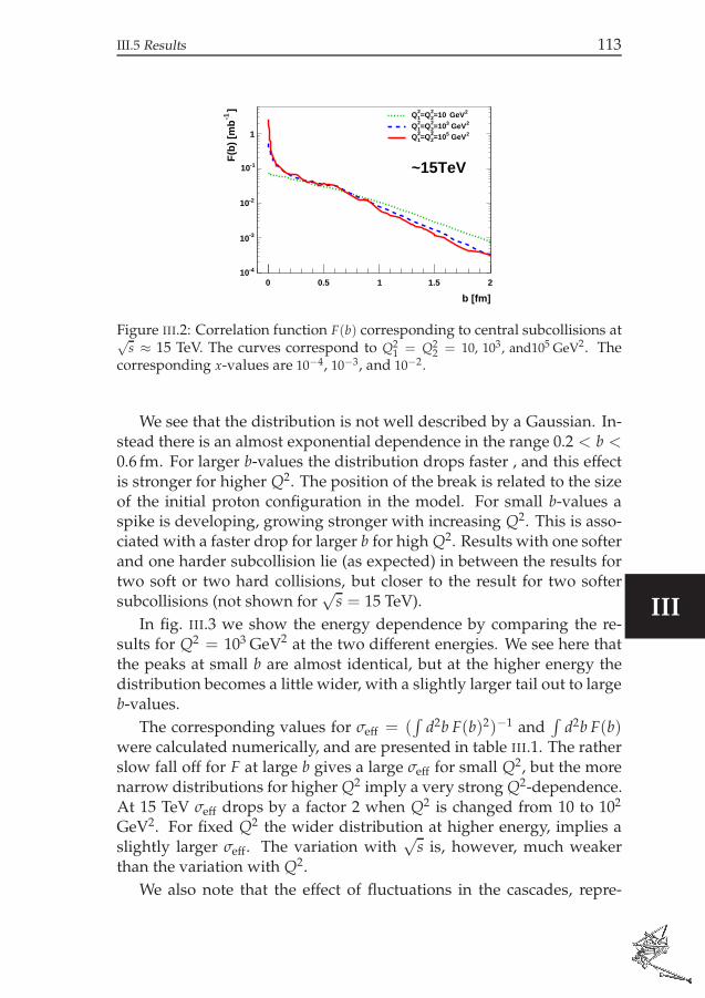
III.5 Results 113
b [fm]
0 0.5 1 1.5 2
]
-1F
(b)
[mb
-410
-310
-210
-110
1
2 GeV =1022=Q1
2Q2 GeV3=102
2=Q12Q
2 GeV5=1022=Q1
2Q
~15TeV
Figure III.2: Correlation function F(b) corresponding to central subcollisions at√s ≈ 15 TeV. The curves correspond to Q2
1 = Q22 = 10, 103, and105 GeV2. The
corresponding x-values are 10−4, 10−3, and 10−2.
We see that the distribution is not well described by a Gaussian. In-stead there is an almost exponential dependence in the range 0.2 < b <
0.6 fm. For larger b-values the distribution drops faster , and this effectis stronger for higher Q2. The position of the break is related to the sizeof the initial proton configuration in the model. For small b-values aspike is developing, growing stronger with increasing Q2. This is asso-ciated with a faster drop for larger b for high Q2. Results with one softerand one harder subcollision lie (as expected) in between the results fortwo soft or two hard collisions, but closer to the result for two softersubcollisions (not shown for
√s = 15 TeV).
In fig. III.3 we show the energy dependence by comparing the re-sults for Q2 = 103 GeV2 at the two different energies. We see here thatthe peaks at small b are almost identical, but at the higher energy thedistribution becomes a little wider, with a slightly larger tail out to largeb-values.
The corresponding values for σeff = (∫
d2b F(b)2)−1 and∫
d2b F(b)were calculated numerically, and are presented in table III.1. The ratherslow fall off for F at large b gives a large σeff for small Q2, but the morenarrow distributions for higher Q2 imply a very strong Q2-dependence.At 15 TeV σeff drops by a factor 2 when Q2 is changed from 10 to 102
GeV2. For fixed Q2 the wider distribution at higher energy, implies aslightly larger σeff. The variation with
√s is, however, much weaker
than the variation with Q2.
We also note that the effect of fluctuations in the cascades, repre-
III

114 Correlations in double parton distributions at small x
b [fm]
0 0.5 1 1.5 2
]
-1F
(b)
[mb
-410
-310
-210
-110
1
2 GeV3=1022=Q1
2Q =1.5 TeVs2 GeV3=102
2=Q12Q =15 TeVs
Figure III.3: The energy dependence of the correlation functions F(b). Thecurves show F for Q2
1 = Q22 = 103 GeV2, solid line for
√s = 1.5 and dashed
line for√
s = 15 TeV.
Q21, Q2
2 [GeV2], x1, x2 σeff [mb]∫
F
1.5 TeV, midrapidity10 10 0.001 0.001 35.3 1.0910 103 0.001 0.01 31.0 1.07103 103 0.01 0.01 23.1 1.06
15 TeV, midrapidity10 10 0.0001 0.0001 40.4 1.11103 103 0.001 0.001 26.3 1.07103 105 0.001 0.01 24.2 1.05105 105 0.01 0.01 19.6 1.03
1.5 TeV, ypair 2 = 2.310 10 0.001 0.000110 10 0.001 0.01
}
37.1 1.08
Table III.1: Summary of results for σeff and corresponding integrals of the dou-ble distribution functions. (The numerical uncertainties are about 1%.)
sented by the difference from 1 of∫
d2b F, is of the order 5-10% (con-tributing 10-20% to σeff), and is smaller for large Q2.
III.5.2 Sub-collisions off midrapidity
As mentioned in sec. III.2.2, for subcollisions away from midrapidity,the effective cross section is given by eq. eq. (III.7) , which contains

III.5 Results 115
b [fm]
0 0.5 1 1.5 2
]
-1F
(b)
[mb
-410
-310
-210
-110
F_S: 2 GeV =1022=Q1
2Q =0.00012=0.001 x1x:CENTRALF 2 GeV=102
2=Q12Q =0.0012=0.001 x1x
F_L: 2 GeV=1022=Q1
2Q =0.012=0.001 x1x
Figure III.4: Correlation function F(b) relevant for subcollisions at ypair 2 = 2.3
for√
s ≈ 1.5 TeV and Q21 = Q2
2 = 10 GeV2. FS ≡ F(b; 0.001, 0.0001, 10, 10) andFL ≡ F(b; 0.001, 0.01, 10, 10). (Q2 in GeV2) The distribution F(b; 0.001, 0.001, 10, 10)
for two subcollisions at midrapidity is included for comparison.
a product of two F-distributions with different x-values. In fig. III.4we show results relevant for two subcollisions with Q2 = 10 GeV2 at1.5 TeV. One collision is at rapidity zero, with x1 = x′1 = 0.001, while theother subcollision has x2 = 0.01 and x′2 = 0.0001, which correspondsto a rapidity for the pair of jets (or a produced massive particle) givenby ypair = ln(x2/x′2)/2 ≈ 2.3. The corresponding F-distributions arecalled FS (for small x2 = 0.0001) and FL (for large x2 = 0.01). We seethat in the tail FS and FL lie on opposite sides of the distribution Fcentral,which is the relevant one for two subcollisions at midrapidity (both withxi = x′i = 0.001). As σeff is given by (
∫
d2bFSFL)−1, this implies that
although the F-distributions vary with x, σeff is approximately indepen-dent of ypair. This result is further illustrated in fig. III.5, which showsthe ratio
√FSFL/Fcentral. We see that this ratio is close to 1 except for
small b-values, which have a low weight in the integral over d2b. Asa consequence also the result for σeff varies very little with rapidity, inthis case from 35.3 to 37.1 mb when ypair is changed from 0 to 2.3 (seetable III.1). Actually, for small shifts δypair, the difference between theproduct FLFS and F2
central must be only second order in δypair. This mustthen also be the case for the corresponding values for σeff.
III.5.3 Comparison with experiment
The result for σeff is larger than the effective cross section observed forγ + 3jet events at the Tevatron. We note, however, that these data de-
III

116 Correlations in double parton distributions at small x
b [fm]
0 0.5 1 1.5 2
C
EN
TR
AL
/ F
S F L
F
0.6
0.8
1
1.2
1.42 GeV =102
2=Q12Q =1.5 TeVs
Figure III.5: The ratio√
FLFS/Fcentral. Q21 = Q2
2 = 10 GeV2, and√
s = 1.5 TeV.
pend on quark distributions, and not only on the gluon distributions.It would be interesting to try to estimate the difference, but this goesbeyond the scope of this paper. For Q2 = 103 GeV2 at 1.5 TeV we findσeff = 23 mb. Within the errors this is in agreement with the 4-jet re-sults from CDF, which however, have large uncertainties. It would alsobe interesting to have, for comparison, the values for σeff in the tunedversions of PYTHIA 8, not only for the less successful single Gaussianapproximation used in section III.2.3.
We also note that there are two observed features, which are wellreproduced by our model:
i. The D0 collaboration [5] has observed a reduction in σeff for grow-ing p⊥ of the jet pair in γ + 3 jet-events. Although the errors are large,
the central values for σeff drop from 18.2 to 13.9 mb, when 〈pjet2T 〉 in-
creases from 17.6 to 27.3 GeV. This agrees qualitatively with the varia-tion with Q2 found in our model.
ii. The CDF collaboration [3] observes in the same reaction, that σeff
is very insensitive to a change in the rapidity ypair (or equivalently xpairF )
for one of the subcollisions. As discussed in sec. III.5.2 this is also con-sistent with our model. We note, however, that this result is mainlya consequence of the fact that the product FL FS is close to F2
central, anddoes not neccesarily show that F does not vary with x.
These qualitative agreements with experimental data may indicatethat, also if our model possibly underestimates the correlations, we maybelieve that the qualitative features, and variations with Q2 and
√s, are
correct. The indicated strong dependence on Q2 should then be very im-

III.6 Conclusions and outlook 117
portant for the interpretation of multiple hard interactions at LHC. Wehere note a possible qualitative difference between our model and themodel with x-dependent matter densities in ref. [16]. Our result showsa larger variation with Q2 for fixed energy, than with x (or energy) forfixed Q2. At fixed energy a variation with Q2 is equivalent to a variationwith x = Q/
√s. However, the two models may give different results
when data at different energies are compared. We would like to studythis question more in the future.
III.5.4 Comment on the definition of b
As mentioned in sec. III.4, in the dipole model F depends in principleon three vectors: the size of the two dipoles (r1, r2) and the separationbetween them. For the results presented above we have defined the sep-aration as the distance between two gluons, and averaged over r1 andr2. When calculating
∫
d2b F(b) this gives exactly the correct result. Thisis, however, not the case for the integral
∫
d2b F2(b), which determinesσeff. When the separation is of the same order of magnitude as the sizeof the dipoles, the averaging does not give the correct result. To estimatethis error we have changed the definition of b, to the separation betweenthe centers of the dipoles, keeping this fixed when averaging over an-gles for r1 and r2. The ratio between the two different F-distributionsis shown in fig. III.6. In this example we have Q2
1 = Q22 = 10 GeV2
and√
s = 15 TeV. We can here see a difference when b is of the sameorder of magnitude as the dipoles, around 0.1 fm. The contributionfrom small b-values is, however, suppressed in the integral over d2b,and as mentioned above
∫
d2b F2(b) obtains its major contribution for bin the range 0.5-1 fm. The difference between the two estimates of σeff
is only about 2.5%. For larger Q2 the difference is even smaller, as theregion where the two b-definitions give different results moves towardssmaller b-values. This effect can therefore be safely neglected.
III.6 Conclusions and outlook
The Lund Dipole Cascade model offers unique possibilities to study theevolution of gluons inside hadrons at small x. The formalism is basedon BFKL evolution including essential higher-order corrections and sat-uration effects. By following the evolution, emission-by-emission, inrapidity and in transverse position, we can investigate the correlationsand fluctuations of the gluon distribution in great detail.
III

118 Correlations in double parton distributions at small x
b [fm]
0 0.5 1 1.5 2
F(b
_gl.s
ep)
/ F(b
_dip
.cen
t)
0.6
0.8
1
1.2
1.42 GeV =102
2=Q12Q
~15TeV
Figure III.6: The ratio between the F-distributions obtained by two differentdefinitions of b. Q2
1 = Q22 = 10 GeV2, and
√s = 15 TeV.
We have here concentrated on the double parton distribution, whichenters into the multiple parton scattering cross section in proton-protoncollisions. The double parton distribution in transverse coordinatespace is the analogy of the generalized parton density in momentumspace. The correlations can be described by a distribution in impactparameter space, F(b; x1, x2, Q2
1, Q22). In many applications this distri-
bution is assumed to be independent of the energy fractions and scalesof the partons, and the same for quarks and gluons. In the PYTHIA 8event generator the width of the distribution does vary with energy,and in a recent study it is assumed to vary with x. Gaunt and Stir-ling have demonstrated that DGLAP evolution implies non-trivial cor-relations depending on x and Q2, but this analysis does not give infor-mation about the b-dependence. In our analysis we find that the two-parton correlation function F(b) depends in a non-trivial way on all thekinematic variables x1, x2, Q2
1, Q22.
For subcollisions at midrapidity, F is directly connected to the “ef-fective cross section” used in experimental analyses, via the relation∫
d2b F2 = σ−1eff . The result that F depends on xi and Q2
i implies, how-ever, that for subcollisions away from y = 0, σeff is determined by anintegral of a product of two F-functions with different x-values, con-nected by the relation xix
′i = Q2/s. Therefore σeff is very insensitive to
the rapidity of a hard subcollision; when one of the two F-functions inthe product is above, the other is below the F-distribution relevant formidrapidity subcollisions. An experimental result showing a weak de-pendence on rapidity is therefore not a proof that F does not depend on

III.6 Conclusions and outlook 119
the scaling parameters xi.
In our formalism we can also study event-by-event fluctuations inthe density of partons, which are usually neglected in other analy-ses. Neglecting the fluctuations F satisfies the normalization condition∫
d2b F = 1, but when taking them into account we obtain a larger valuefor this integral, and therefore larger two-parton correlations. In ouranalysis this effect contributes 10-20% to the value of σeff.
By studying the correlation function F, we can see explicitly how theemission of high-p⊥ gluons result in so-called hot spots developing forsmall b-values at large Q2. For fixed Q2 the emission of larger dipoles,related to low-p⊥ gluons, implies that the distribution widens as we godown in x. (This effect is related to the shrinking of the diffractive peakat higher energies.) As a result σeff is reduced for higher Q2 at fixedenergy, but increases at higher energy for fixed Q2. We see, however,that the result appears to depend much stronger on Q2 than on x orcollision energy.
It is not straight-forward to compare our results for the effectivecross section with data from the Tevatron and ISR, which correspond tolower values for σeff and thus stronger correlations. The ISR data are ob-tained for very high x-values, and the more exact Tevatron results are forγ + 3 jet events, which necessarily involves quarks. Our calculations in-clude only gluons, and should therefore only be applied at small x. It isalso difficult to estimate a possible difference between quark and gluondistributions. Our results are, however, compatible within errors withthe four-jet measurement at CDF, where gluons should be dominating,and they show qualitative agreements with the observed rapidity inde-pendence at CDF and the hints of strong Q2-dependence at D0. We alsonote that our results appear to be in qualitative agreement with resultsfrom PYTHIA 8 tuned to multiple interactions and underlying events.
Even if it is possible that we overestimate the result for σeff to somedegree, we are more confident about the variation with x and Q2, whichshould have relevance for extrapolations to the LHC. Our model herepredicts a very strong decrease of the effective cross section with in-creasing Q2 (especially when both Q2
1 and Q22 increases), while the de-
pendence on the total energy (∼ 1/x) for fixed Q2 is rather weak. Alsothe dependence on the rapidity of the two subcollisions is quite weak,which follows as σeff here is given by a product of two F-distribution,one which is smaller and one which is larger than the F-distributionrelevant for midrapidity subcollisions.
When comparing to the recent option in PYTHIA 8, with an x-
III

120 Correlations in double parton distributions at small x
dependent impact parameter profile [16], our result may be quite simi-lar if we study the dependence on Q2 at a fixed cms energy
√s. In our
model the correlations increase as a direct consequence of higher Q2,and in the PYTHIA 8 model they increase because x is higher for large Q2
at fixed energy. The difference between the two models might thereforeshow up in the extrapolation of Tevatron data to LHC energies.
It should be noted, however, that the extraction of the effective crosssections from data is very hard, and it will still be difficult to comparefuture LHC results to the numbers we have presented here. For this rea-son it is important to compare to event generator predictions for the ex-perimental observables. Fortunately we have now developed the DIPSY
MC to also generate exclusive final states [41], which means that in thefuture we can in detail simulate exclusive final state observables relatedto double parton scattering.
Acknowledgments
Work supported in part by the EU Marie Curie RTN MCnet (MRTN-CT-2006-035606), and the Swedish research council (contracts 621-2008-4252and 621-2009-4076).
L.L. gratefully acknowledges the hospitality of the CERN theoryunit.
A.S. gratefully acknowledges the support of the Hungarian OTKAgrants T49466 and NK 73143.

III References 121
III References
[1] Axial Field Spectrometer Collaboration, T. Akesson et al.,“DOUBLE PARTON SCATTERING IN p p COLLISIONS ATS**(1/2) = 63-GeV,” Z. Phys. C34 (1987) 163.
[2] CDF Collaboration, F. Abe et al., “Study of four jet events andevidence for double parton interactions in pp collisions at√
s = 1.8 TeV,” Phys. Rev. D47 (1993) 4857–4871.
[3] CDF Collaboration, F. Abe et al., “Double parton scattering in ppcollisions at
√s = 1.8TeV,” Phys. Rev. D56 (1997) 3811–3832.
[4] D0 Collaboration, V. M. Abazov et al., “Multiple jet production atlow transverse energies in pp collisions at
√s = 1.8 TeV,” Phys.
Rev. D67 (2003) 052001, arXiv:hep-ex/0207046.
[5] D0 Collaboration, V. M. Abazov et al., “Double parton interactionsin photon+3 jet events in p p- bar collisions sqrts=1.96 TeV,” Phys.Rev. D81 (2010) 052012, arXiv:0912.5104 [hep-ex].
[6] J. Kuti and V. F. Weisskopf, “Inelastic lepton - nucleon scatteringand lepton pair production in the relativistic quark partonmodel,” Phys. Rev. D4 (1971) 3418–3439.
[7] V. P. Shelest, A. M. Snigirev, and G. M. Zinovev, “THEMULTIPARTON DISTRIBUTION EQUATIONS IN QCD,” Phys.Lett. B113 (1982) 325.
[8] T. Sjostrand and M. van Zijl, “A Multiple Interaction Model for theEvent Structure in Hadron Collisions,” Phys. Rev. D36 (1987) 2019.
[9] T. T. Chou and C. N. Yang, “GEOMETRICAL MODEL OFMULTIPARTICLE PRODUCTION IN HADRON - HADRONCOLLISIONS,” Phys. Rev. D32 (1985) 1692.
[10] A. M. Snigirev, “Double parton distributions in the leadinglogarithm approximation of perturbative QCD,” Phys. Rev. D68
(2003) 114012, arXiv:hep-ph/0304172.
[11] J. R. Gaunt and W. J. Stirling, “Double Parton DistributionsIncorporating Perturbative QCD Evolution and Momentum andQuark Number Sum Rules,” JHEP 03 (2010) 005,arXiv:0910.4347 [hep-ph].
III

122 Correlations in double parton distributions at small x
[12] T. Sjostrand and P. Z. Skands, “Multiple interactions and thestructure of beam remnants,” JHEP 03 (2004) 053,arXiv:hep-ph/0402078.
[13] T. Sjostrand and P. Z. Skands, “Transverse-momentum-orderedshowers and interleaved multiple interactions,” Eur. Phys. J. C39
(2005) 129–154, arXiv:hep-ph/0408302.
[14] T. Sjostrand, S. Mrenna, and P. Z. Skands, “A Brief Introduction toPYTHIA 8.1,” Comput. Phys. Commun. 178 (2008) 852–867,arXiv:0710.3820 [hep-ph].
[15] T. Sjostrand, S. Mrenna, and P. Z. Skands, “PYTHIA 6.4 Physicsand Manual,” JHEP 05 (2006) 026, arXiv:hep-ph/0603175.
[16] R. Corke and T. Sjostrand, “Multiparton Interactions with anx-dependent Proton Size,” arXiv:1101.5953 [hep-ph].
[17] M. Bahr, S. Gieseke, and M. H. Seymour, “Simulation of multiplepartonic interactions in Herwig++,” JHEP 07 (2008) 076,arXiv:0803.3633 [hep-ph].
[18] M. Bahr, J. M. Butterworth, S. Gieseke, and M. H. Seymour, “Softinteractions in Herwig++,” arXiv:0905.4671 [hep-ph].
[19] M. Bahr et al., “Herwig++ Physics and Manual,” Eur. Phys. J. C58
(2008) 639–707, arXiv:0803.0883 [hep-ph].
[20] E. A. Kuraev, L. N. Lipatov, and V. S. Fadin, “The PomeranchukSingularity in Nonabelian Gauge Theories,” Sov. Phys. JETP 45
(1977) 199–204.
[21] I. I. Balitsky and L. N. Lipatov, “The Pomeranchuk Singularity inQuantum Chromodynamics,” Sov. J. Nucl. Phys. 28 (1978) 822–829.
[22] E. Avsar, G. Gustafson, and L. Lonnblad, “Energy conservationand saturation in small-x evolution,” JHEP 07 (2005) 062,arXiv:hep-ph/0503181.
[23] E. Avsar, G. Gustafson, and L. Lonnblad, “Small-x dipoleevolution beyond the large-N(c) limit,” JHEP 01 (2007) 012,arXiv:hep-ph/0610157.
[24] E. Avsar, G. Gustafson, and L. Lonnblad, “Difractive Excitation inDIS and pp Collisions,” JHEP 12 (2007) 012, arXiv:0709.1368[hep-ph].

III References 123
[25] C. Flensburg, G. Gustafson, and L. Lonnblad, “Elastic andquasi-elastic pp and γ∗p scattering in the Dipole Model,” Eur.Phys. J. C60 (2009) 233–247, arXiv:0807.0325 [hep-ph].
[26] C. Flensburg and G. Gustafson, “Fluctuations, Saturation, andDiffractive Excitation in High Energy Collisions,” JHEP 10 (2010)014, arXiv:1004.5502 [hep-ph].
[27] A. H. Mueller, “Soft gluons in the infinite momentum wavefunction and the BFKL pomeron,” Nucl. Phys. B415 (1994) 373–385.
[28] A. H. Mueller and B. Patel, “Single and double BFKL pomeronexchange and a dipole picture of high-energy hard processes,”Nucl. Phys. B425 (1994) 471–488, hep-ph/9403256.
[29] A. H. Mueller, “Unitarity and the BFKL pomeron,” Nucl. Phys.B437 (1995) 107–126, hep-ph/9408245.
[30] B. Blok, Y. Dokshitzer, L. Frankfurt, and M. Strikman, “The four jetproduction at LHC and Tevatron in QCD,” arXiv:1009.2714
[hep-ph].
[31] G. P. Salam, “An introduction to leading and next-to-leadingBFKL,” Acta Phys. Polon. B30 (1999) 3679–3705, hep-ph/9910492.
[32] I. Balitsky and G. A. Chirilli, “NLO evolution of color dipole,”Acta Phys. Polon. B39 (2008) 2561–2566.
[33] A. H. Mueller and G. P. Salam, “Large multiplicity fluctuationsand saturation effects in onium collisions,” Nucl. Phys. B475 (1996)293–320, hep-ph/9605302.
[34] J. Kwiecinski, A. D. Martin, and P. J. Sutton, “Constraints on gluonevolution at small x,” Z. Phys. C71 (1996) 585–594,hep-ph/9602320.
[35] E. Iancu, A. Leonidov, and L. McLerran, “The Color glasscondensate: An Introduction,” arXiv:hep-ph/0202270 [hep-ph].
[36] E. Iancu and R. Venugopalan, “The Color glass condensate andhigh-energy scattering in QCD,” arXiv:hep-ph/0303204
[hep-ph]. To be published in QGP3, Eds. R.C. Hwa andX.N.Wang, World Scientific.
III

124 Correlations in double parton distributions at small x
[37] F. Gelis, E. Iancu, J. Jalilian-Marian, and R. Venugopalan, “TheColor Glass Condensate,” arXiv:1002.0333 [hep-ph]. *Temporary entry *.
[38] E. Iancu, A. Leonidov, and L. D. McLerran, “Nonlinear gluonevolution in the color glass condensate. 1.,” Nucl.Phys. A692 (2001)583–645, arXiv:hep-ph/0011241 [hep-ph].
[39] J. Jalilian-Marian, A. Kovner, A. Leonidov, and H. Weigert, “TheBFKL equation from the Wilson renormalization group,”Nucl.Phys. B504 (1997) 415–431, arXiv:hep-ph/9701284[hep-ph].
[40] E. Avsar, “On the High Energy Behaviour of The Total CrossSection in the QCD Dipole Model,” JHEP 04 (2008) 033,arXiv:0803.0446 [hep-ph].
[41] C. Flensburg, G. Gustafson, and L. Lonnblad, “Inclusive andExclusive observables from dipoles in high energy collisions,”arXiv:1103.4321 [hep-ph].
IV
Inclusive and Exclusive observables from
dipoles in high energy collisions
Christoffer Flensburg1, Gosta Gustafson1, Leif Lonnblad1,2
1Dept. of Astronomy and Theoretical Physics, Lund University,Sweden
2CERN Theory Department, Geneva, Switzerland
LU-TP 11-13CERN-PH-TH-2011-058
MCnet-11-08e-Print: [arXiv:1103.4321]
We present a new model for simulating exclusive final states in minimum-biascollisions between hadrons.
In a series of papers we have developed a Monte Carlo model based onMueller’s dipole picture of BFKL-evolution, supplemented with non-leadingcorrections, which has shown to be very successful in describing inclusive andsemi-inclusive observables in hadron collisions. In this paper we present afurther extension of this model to also describe exclusive final states. Thisis a highly non-trivial extension, and we have encountered many details thatinfluence the description, and for which no guidance from perturbative QCDcould be found. Hence we have had to make many choices based on semi-classical and phenomenological arguments.
The end result is a new event generator called DIPSY which can be used
to simulate complete minimum-bias non-diffractive hadronic collision events.
Although the description of data from the Tevatron and LHC is not quite as
good as for PYTHIA 8, the most advanced of the general purpose event gen-
erator programs for these processes, our results are clearly competitive, and
can be expected to improve with careful tuning. In addition, as our model is
very different from conventional multiple scattering scenaria, the DIPSY pro-
gram can be used to gain deeper insight in the soft and semi-hard processes
involved both in hadronic and heavy ion collisions.
IV

126 Inclusive and Exclusive observables from dipoles in high energy collisions
IV.1 Introduction
In high energy collisions the high density of gluons at small x imply thattypical events contain several hard partonic subcollisions, and that sat-uration effects become important. A dynamical model based on BFKLevolution [1, 2] for small x and including saturation effects, has beenpresented in a series of papers [3–7]. It is based on Mueller’s dipolecascade model [8–10], which is a formulation of the leading logarithmic(LL) BFKL evolution approximation in impact-parameter space. In ourmodel we also include essential beyond LL corrections to BFKL. Thetransverse coordinate space is particularly suitable for treating unitarityconstraints, multiple collisions, and saturation effects. Mueller’s modelincludes multiple subcollisions in the frame used for the analysis. Ourcascade model also includes saturation effects within the parton evolu-tion, in a way which is similar to the Color Glass Condensate [11–13] orJIMWLK [14, 15]. Also effects of confinement are included and impor-tant for the result.
In the dipole picture the colour charge in a gluon is screened by acorresponding anticharge in a neighbouring gluon. Gluon radiation im-plies that one dipole is split in two dipoles, and the result of the cascadeis a chain of colour connected gluons. When two cascades collide, thecan interact via gluon exchange. This implies an exchange of colour,producing two colour chains forming a BFKL ladder between projec-tile and target. Multiple interaction and saturation represent multiplepomeron exchange and pomeron loops. Note here that what is multi-ple interaction in one Lorentz frame is related to saturation within thecascade in another frame.
The BFKL formalism is directly applicable to inclusive observables,and the cited articles include results for total, (quasi)elastic, and diffrac-tive cross sections in pp scattering and in DIS, in very good agreementwith experimental data. The numerical results are obtained with aMonte Carlo (MC) event generator called DIPSY1.
In the present paper we want to generalize the model to describeexclusive final states. Here it is necessary to take into account colourcoherence and angular ordering as well as soft radiation. The latterincludes contributions from the z = 1 singularity in the gluon split-ting function. These effects are taken into account in the CCFM for-malism [16,17], which also reproduces the BFKL result for the inclusivecross section. In ref. [18], describing the Linked Dipole Chain model, it
1Acronym for Dipoles in Impact-Parameter Space and rapidity (Y)

IV.1 Introduction 127
P
k0q1
k1
q2
k2
q3
Figure IV.1: A chain of initial state gluon emissions. We denote the real emittedgluons in a gluon ladder q⊥i, and the virtual links k⊥i.
was demonstrated that the inclusive cross section is fully determined bya subset of the gluons in the CCFM approach, denoted “k⊥-changing”gluons. As illustrated in fig. IV.1, we denote the real emitted gluonsin a gluon ladder q⊥i, and the virtual links k⊥i. Momentum conserva-tion here implies that k⊥i−1 = k⊥i + q⊥i. In a k⊥-changing emissionthe difference is large between two adjacent virtual links, k⊥i−1 and k⊥i.This means that q⊥i ≈ max(k⊥i−1, k⊥i). Softer emissions with smallerq⊥i have k⊥i−1 ≈ k⊥i, and are “k⊥-conserving”. In CCFM gluon emis-sion is associated with “non-Sudakov” form factors, and in ref. [18]it was demonstrated that these gluons can be summed up in such away, that the total cross section is fully specified by the k⊥-changingemissions with no associated non-Sudakov form factors. The remain-ing k⊥-changing gluons q
prim⊥i are called “primary gluons” in ref. [18]
and “backbone gluons” in ref. [19]. They are ordered in both lightconevariables q+ and q−, and therefore also in rapidity or angle, in accor-dance with QCD coherence. (In the LDC model [18] emissions withk⊥i ≈ k⊥i−1, on the boundary between k⊥-conserving and k⊥-changingemissions, were treated slightly different from the BFKL prescription,which also implied a slightly different value for the exponent λ in thepower-like increase ∝ 1/xλ. In the present model the LL BFKL result isexactly reproduced.)
The chains of primary gluons also determine the structure of the finalstate, but as discussed above, to get the full exclusive states softer emis-sions must be added as final state radiation. In summary the generationof exclusive final states contains the following steps:
IV

128 Inclusive and Exclusive observables from dipoles in high energy collisions
1. The generation of two dipole cascades from the projectile and thetarget, in accordance with BFKL dynamics and saturation.
2. Calculating which pairs of one parton in the projectile and oneparton in the target do interact. In BFKL the emission of gluons isa Poissonian type process, and the interaction probability is calcu-lated in the eikonal approximation.
3. Extracting the primary, k⊥-changing, gluons, and checking thatthey are given the correct weight. These gluons form colourconnected chains between the projectile and the target, includ-ing branchings and loops. This step includes the removal ofbranches in the cascade which do not interact, and restoringenergy-momentum conservation.
4. Adding final state radiation in relevant parts of phase space. Theresult consists of chains of colour connected gluons.
5. Hadronization. Here we use Lund string hadronization, wherecolour strings are stretched between the colour-connected gluons.
The outline of the paper is as follows: In section IV.2 we describeour dipole cascade model for inclusive observables. The problems en-countered when generating exclusive final states are discussed in sec-tion IV.3. In section IV.4 we describe the key procedures used in theMC for solving the problems presented in section IV.3, while some ofthe more technical details are left for the appendices. Some results andpredictions are given in section IV.5, together with a discussion of tun-able parameters in the program. Finally our conclusions are given insection IV.6.
IV.2 The Lund dipole cascade model for inclusive
cross sections
IV.2.1 Mueller’s cascade model and the eikonal formalism
Mueller’s dipole cascade model [8–10] is a formulation of LL BFKL evo-lution in transverse coordinate space. Gluon radiation from the colourcharge in a parent quark or gluon is screened by the accompanying an-ticharge in the colour dipole. This suppresses emissions at large trans-verse separation, which corresponds to the suppression of small k⊥ inBFKL. For a dipole (x, y) the probability per unit rapidity (Y) for emis-
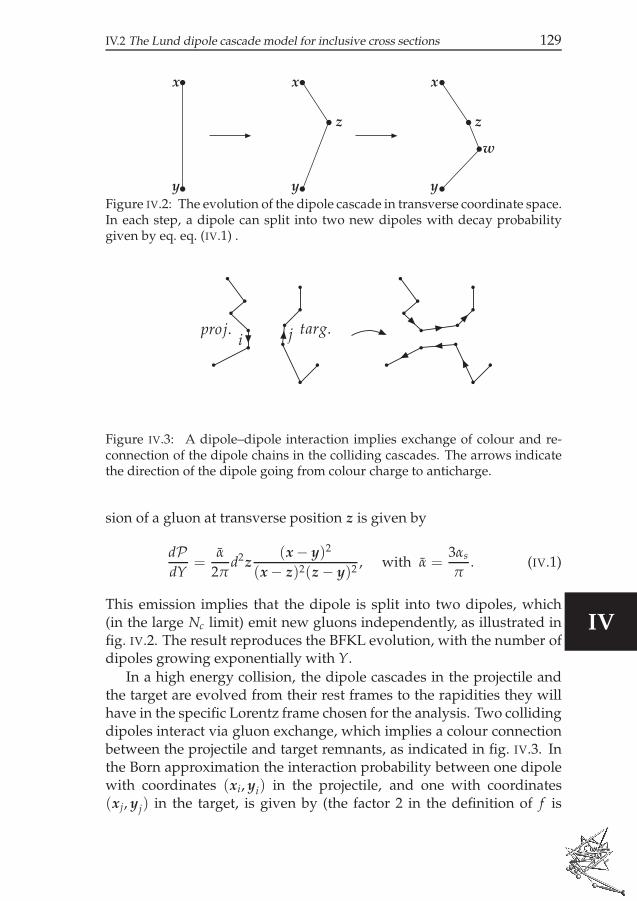
IV.2 The Lund dipole cascade model for inclusive cross sections 129
x
y
x
y
z
x
y
z
w
Figure IV.2: The evolution of the dipole cascade in transverse coordinate space.In each step, a dipole can split into two new dipoles with decay probabilitygiven by eq. eq. (IV.1) .
i jproj. targ.
Figure IV.3: A dipole–dipole interaction implies exchange of colour and re-connection of the dipole chains in the colliding cascades. The arrows indicatethe direction of the dipole going from colour charge to anticharge.
sion of a gluon at transverse position z is given by
dPdY
=α
2πd2z
(x − y)2
(x − z)2(z − y)2, with α =
3αs
π. (IV.1)
This emission implies that the dipole is split into two dipoles, which(in the large Nc limit) emit new gluons independently, as illustrated infig. IV.2. The result reproduces the BFKL evolution, with the number ofdipoles growing exponentially with Y.
In a high energy collision, the dipole cascades in the projectile andthe target are evolved from their rest frames to the rapidities they willhave in the specific Lorentz frame chosen for the analysis. Two collidingdipoles interact via gluon exchange, which implies a colour connectionbetween the projectile and target remnants, as indicated in fig. IV.3. Inthe Born approximation the interaction probability between one dipolewith coordinates (xi, yi) in the projectile, and one with coordinates(xj, yj) in the target, is given by (the factor 2 in the definition of f is
IV

130 Inclusive and Exclusive observables from dipoles in high energy collisions
a convention)
2 fij = 2 f (xi, yi|xj, yj) =α2
s
4
[
log
( (xi − yj)2(yi − xj)
2
(xi − xj)2(yi − yj)2
)]2
. (IV.2)
At high energies the strong increase in the number of dipoles gives alarge probability for multiple dipole–dipole subcollisions, and the trans-verse coordinate space is particularly suitable for the treatment of mul-tiple interactions and unitarity constraints. Assuming that the subcolli-sions are uncorrelated, multiple collisions are taken into account in theeikonal approximation, where the probability for an inelastic interactionis given by
Int. prob. = 1 − e−2F, with F = ∑ fij. (IV.3)
The multiple interactions produce loops of dipole chains, correspondingto the pomeron loops in the reggeon formalism.
Assuming also that the elastic scattering amplitude, T, is driven byabsorption into inelastic states, we find via the optical theorem
T = 1 − e−F, (IV.4)
and thus the probability for an elastic interaction given by T2. (We usea definition such that T in this case is purely real.)
To get the final result for the proton–proton cross sections we have totake averages over the projectile and target cascades, and integrate overimpact parameter b. For the total non-diffractive cross section we get
σinel =∫
d2b〈1 − e−2F(b)〉 =∫
d2b〈1 − (1 − T(b))2〉. (IV.5)
When the projectile has an internal structure, which can be excited, thepurely elastic cross section is obtained by taking the average of the am-plitude T, before taking the square:
σel =∫
d2b〈T(b)〉2. (IV.6)
Taking first the square gives the total diffractive scattering (see ref. [20]):
σdiff =∫
d2b〈T(b)2〉. (IV.7)
The cross section for diffractive excitation is consequently given by thedifference
σdiff ex = σdiff − σel =∫
d2b(
〈T(b)2〉 − 〈T(b)〉2)
. (IV.8)

IV.2 The Lund dipole cascade model for inclusive cross sections 131
Thus diffractive excitation is determined by the fluctuations in the scat-tering amplitude. It is also possible to calculate e.g. the cross sectionfor single diffractive excitation of the (right-moving) projectile by tak-ing the average over the target cascade before, but over the projectilecascade after, squaring the amplitude. We also here have to subtract theelastic scattering, and thus get
σSD =∫
d2b(
〈〈T(b)〉2L〉R − 〈T(b)〉2
)
, (IV.9)
where 〈·〉L(R) refers to the average over the left (right) cascade only.
IV.2.2 The Lund dipole cascade model
The Lund dipole cascade introduces a number of corrections toMueller’s original formulation. They are all beyond the leading log-arithmic approximation. While some of them correspond to the next-to-leading (NLL) corrections, others are not possible to completely as-sociate with a given order in the perturbative logarithmic expansion,and we therefore simply denote them beyond leading order. The correc-tions are described in greater detail in previous articles [3–5], and a shortsummary is presented here.
Beyond LL BFKL evolution
The NLL corrections to BFKL evolution have three major sources [21]:
Non-singular terms in the splitting function:These terms suppress large z-values in the individual parton branch-
ings, and prevent the child from being faster than its recoiling parent.Most of this effect is taken care of by including energy-momentum con-servation in the evolution. This is effectively taken into account by as-sociating a dipole with transverse size r with a transverse momentumk⊥ = 1/r, and demanding conservation of the lightcone momentum p+
in every step in the evolution. This gives an effective cutoff for smalldipoles, which eliminates the numerical problems encountered in theMC implementation by Mueller and Salam [22].
Projectile-target symmetry:A parton chain should look the same if generated from the target end
as from the projectile end. The corresponding corrections are also calledenergy scale terms, and is essentially equivalent to the so called consis-tency constraint [23]. This effect is taken into account by conservation of
IV

132 Inclusive and Exclusive observables from dipoles in high energy collisions
both positive and negative lightcone momentum components, p+ andp−.
The running coupling:
This is relatively easily included in a MC simulation process. Thescale in the running coupling is chosen as the largest transverse mo-mentum in the vertex, in accordance with the results in ref. [24].
The treatment of these effects includes also effects beyond NLL, in away similar to the treatment by Salam in ref. [21]. Therefore the powerλeff, determining the growth for small x, is not negative for large valuesof αs.
Non-linear effects and saturation
As mentioned above, multiple interactions produce loops of dipolechains corresponding to pomeron loops. Mueller’s model includes allloops cut in the particular Lorentz frame used for the analysis, but notloops contained within the evolution of the individual cascades. As fordipole scattering the probability for such loops is given by αs, and there-fore formally colour suppressed compared to dipole splitting, which isproportional to α = Ncαs/π. These loops are therefore related to theprobability that two dipoles have the same colour. Two dipoles with thesame colour form a quadrupole field. Such a field may be better approx-imated by two dipoles formed by the closest colour–anticolour charges.This corresponds to a recoupling of the colour dipole chains. We callthis process a dipole “swing”. In the MC, dipoles with the same colourare allowed to swing with a probability proportional to (r2
1r22)/(r2
3r24),
where r1 and r2 are the sizes of the original dipoles and r3 and r4 arethe sizes of the recoupled dipoles. Dipoles with the same colour are al-lowed to swing back and forth, which results in an equilibrium, wherethe smaller dipoles have a larger weight. We note that in this formu-lation the number of dipoles is not reduced. The given weights favourthe formation of smaller dipoles, and the saturation effect is obtainedbecause the smaller dipoles have smaller cross sections.
Confinement effects
Confinement effects are included via an effective gluon mass, whichgives an exponential suppression for very large dipoles [5]. This pre-vents the proton from growing too fast in transverse size, and is alsoessential to satisfy Froisart’s bound at high energies [25].

IV.3 From inclusive to exclusive observables 133
IV.2.3 Initial dipole configurations
In DIS an initial photon is split into a qq pair, and for larger Q2 the wave-function for a virtual photon can be determined perturbatively. The in-ternal structure of the proton is, however, governed by soft QCD, and isnot possible to calculate perturbatively. In our model it is representedby an equilateral triangle formed by three dipoles, and with a radiusof 3 GeV−1 ≈ 0.6 fm. The model should be used at low x, and whenthe system is evolved over a large rapidity range the observable resultsdepend only weakly on the exact configuration of the initial dipoles, orwhether the charges are treated as (anti)quarks or gluons.
IV.3 From inclusive to exclusive observables
In this section we discuss the necessary steps when going from inclusiveobservables to exclusive final states. The technical details of the MCimplementation are left to sec. IV.4 and the appendices.
IV.3.1 The chain of k⊥-changing gluons
In the introduction we discussed briefly how the structure of an exclu-sive final state is determined by a backbone of gluons. The first stepis therefore to extract this backbone chain of k⊥-changing or primarygluons, with their proper weights. As discussed above, the differentsubcollisions are assumed to be uncorrelated, and the interaction prob-ability for two dipoles, i and j, is given by 1 − exp(−2 fij), with fij givenby eq. eq. (IV.2) . When the interacting dipoles are determined, the back-bone chains can be found by tracing their parents and previous ances-tors backwards in rapidity. A resulting chain is shown in fig. IV.4a, andwe here use the notation qi for the real emitted gluons, and ki for thevirtual links in the evolution. The same chain is presented in fig. IV.4bin a (y, ln q2
⊥) diagram, with y being the rapidity. In this plot ln q+ andln q− (= y ± ln k⊥) increase towards the upper right and upper left cor-ners. Due to the “consistency constraint” [23], which is part of the NLLcorrections to BFKL, the primary gluons are ordered not only in q+, butalso in q−. This also implies an ordering in rapidity or angle, in ac-cordance with QCD coherence. The real emissions satisfy the relationqi+qi− = q2
i⊥, and are represented by points in fig. IV.4b. The space-likemomenta for the virtual links ki are not constrained by such a relation,and are represented by horizontal lines indicating their transverse mo-mentum.
IV

134 Inclusive and Exclusive observables from dipoles in high energy collisions
The weight for a particular chain with (real) gluons qi is given by[18, 19] (assuming k⊥0 = k⊥n = 0)
∏i
α
π
d2q⊥i
q2⊥i
dyiδ(Σq⊥i), with α ≡ NCαs
π. (IV.10)
We note in particular that this expression is symmetric under exchangeof projectile and target. The result can also be expressed in terms of thevirtual links ki. We then have
n
∏i=1
d2q⊥iδ(Σq⊥i) =n−1
∏i=1
d2k⊥i, (IV.11)
and transverse momentum conservation implies that we have two dif-ferent cases:
1. Step up: k⊥i ≈ q⊥i ≫ k⊥i−1, with weight d2q⊥i/q2⊥i ≈ d2k⊥i/k2
⊥i.
2. Step down: k⊥i ≪ q⊥i ≈ k⊥i−1, with weight d2q⊥i/q2⊥i ≈
d2k⊥i/k2⊥i−1 = d2k⊥i/k2
⊥i × k2⊥i/k2
⊥i−1.
Thus steps down in k⊥ are suppressed by a factor k2⊥i/k2
⊥i−1. This im-plies that links with a local maximum k⊥, as k3 in fig. IV.4, is given theweight d2k⊥i/k4
⊥i, and can be interpreted as a hard scattering betweenk2 and k4, producing the two high-p⊥ gluons q3 and q4. For a link withk⊥ lower than the adjacent real gluons, like k4 in fig. IV.4, the transversemomentum of the real gluons will be determined by the neighbouringlinks k3 and k5. Thus in such cases the associated weight will be d2k⊥i,which is non-singular for small k⊥. Note that no particular rest frameis specified for the collision between the two cascades. The result is thesame if the “hard subcollision” is part of the projectile or target evolu-tion, and thus independent of the Lorentz frame used for the analysis.
IV.3.2 Reabsorption of virtual emissions
A dipole cascade generates a chain of dipoles linked together by glu-ons. A dipole–dipole interaction via gluon exchange implies exchangeof colour, and the chains are recoupled as shown in fig. IV.3. Multipleinteractions produce dipole loops as illustrated in the schematic picturein fig. IV.5. In this example two cascades are evolved in rapidity up tothe dashed line in the center. Here three dipole pairs interact, formingtwo dipole loops. In a projectile cascade with a large lightcone momen-tum p+, and initially small p−, the partons need a contribution of p−
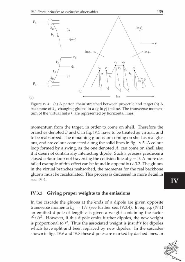
IV.3 From inclusive to exclusive observables 135
Pa
k0q1
k1
q2
k2
q3
qn−1
kn−1
qnkn
Pb
(a)
q6
k5
q5
k4
q4
k3
q3
k2
q2
k1q1
ln q2⊥
y
ln s
ln q+ln q−
(b)
Figure IV.4: (a) A parton chain stretched between projectile and target.(b) Abackbone of k⊥-changing gluons in a (y, ln q2
⊥) plane. The transverse momen-tum of the virtual links ki are represented by horizontal lines.
momentum from the target, in order to come on shell. Therefore thebranches denoted B and C in fig. IV.5 have to be treated as virtual, andto be reabsorbed. The remaining gluons are coming on shell as real glu-ons, and are colour-connected along the solid lines in fig. IV.5. A colourloop formed by a swing, as the one denoted A, can come on shell alsoif it does not contain any interacting dipole. Such a process produces aclosed colour loop not traversing the collision line at y = 0. A more de-tailed example of this effect can be found in appendix IV.3.2. The gluonsin the virtual branches reabsorbed, the momenta for the real backbonegluons must be recalculated. This process is discussed in more detail insec. IV.4.
IV.3.3 Giving proper weights to the emissions
In the cascade the gluons at the ends of a dipole are given oppositetransverse momenta k⊥ = 1/r (see further sec. IV.3.4). In eq. eq. (IV.1)an emitted dipole of length r is given a weight containing the factord2r/r2. However, if this dipole emits further dipoles, the new weightis proportional to r2. Thus the associated weight is just d2r for dipoleswhich have split and been replaced by new dipoles. In the cascadesshown in figs. IV.6 and IV.8 these dipoles are marked by dashed lines. In
IV

136 Inclusive and Exclusive observables from dipoles in high energy collisions
A
C
Br
rapidity
Figure IV.5: Collision of two dipole cascades in r-rapidity space. The dashedvertical line symbolizes the Lorentz frame in which the collision is viewed. Thedipole splitting vertex can result in the formation of different dipole branches,and loops are formed due to multiple sub-collisions. The loop denoted by A isan effect of saturation within the cascade evolution, which can be formed via adipole swing. Branches which do not interact, like those denoted B and C areto be treated as virtual, and to be absorbed.
the following they will be referred to as “inner dipoles”. The remainingdipoles, formed by colour-connected gluons, are marked by heavy lines,and they all get a weight proportional to 1/r2. They will be referred toas “outer dipoles”.
Let us study the cascade shown in fig. IV.6, obtained after the ab-sorption of the virtual gluons as described in the previous subsection.The cascade starts from the dipole (01), followed by emission of gluons2, 3, etc. Here the dipoles are first smaller and smaller, a ≫ b ≫ c ≫ d.The corresponding k⊥-values therefore become larger and larger in eachstep. After the minimum dipole, with size d, the subsequent emissions,5, and 6, give again larger dipoles with correspondingly lower k⊥ val-ues. The weight containing factors 1/r2 for all “remaining dipoles” isproportional to
d2r2
b2· d2r3
c2· d2r4
d0· d2r5
e2· d2r6
f 2· 1
f 2. (IV.12)
In this event gluons 3 and 4 recoil against each other with large trans-verse momenta kmax = 1/d. As all factors of d have canceled ineq. eq. (IV.12) , this gives the proper weight d2r4 ∝ d2kmax/k4
max. Thisreproduces exactly the proper weight for a hard gluon–gluon scattering.

IV.3 From inclusive to exclusive observables 137
a
≈ a
0 ≈ bb
1
2
3
4 5
6
c
cd
e
e
f
Figure IV.6: A dipole cascade in r⊥-space, in which a chain of smaller andsmaller dipoles is followed by a set of dipoles with increasing sizes. The ini-tial dipole between points 0 and 1 is marked by long dashes. Those dipoleswhich have split into two new dipoles, and thus disappeared from the chain,are marked by short dashes. The shortest dipole (34) corresponds to the maxi-mum k⊥, and represents a hard sub-collision.
0 1
2
1’
2’
3
4 3’
5
6 rapidity
ln qT
2
Figure IV.7: The same cascade as in fig. IV.7. The x direction shows rapid-ity, and y direction shows ln(k2
⊥). The diagonal line is the constant p+ of theincoming particle.
The same cascade is shown in fig. IV.7 in the (y, ln(k2⊥)) diagram of
fig. IV.4b. In this figure new emissions are first denoted by open circles,while filled circles mark their position after recoil from a later emission.Thus gluon 1 starts at the lower right corner. After the emission of gluon2, it is recoiling to the position marked 1′. Similarly gluon 2 is shifted toposition 2′, when it emits gluon 3. When gluon 4 emits the softer gluon5, its recoil is small and it keeps its position in the diagram.
Figure IV.8 shows instead a chain with increasing dipole sizes upto a maximum value, rmax, which thus corresponds to a minimumtransverse momentum, kmin. Here we also get the correct weightd2rmax/r4
max ∝ d2kmin, which implies that there is no singularity forsmall k⊥-values. Note that all gluons connected to the long dipoles arealso connected to shorter dipoles, which determine most of their trans-verse momentum. Thus no gluon has q⊥ represented by kmin.
IV

138 Inclusive and Exclusive observables from dipoles in high energy collisions
0
1
2
4
5
3
a
a
bb
b
cc d
Figure IV.8: A cascade where the dipole sizes increase to a maximum, and thendecrease. Here the size of the largest dipole, denoted b, corresponds to theminimum k⊥ in the chain.
IV.3.4 Going from transverse coordinate space to momentumspace
Cascade evolution
The dipole picture is formulated in transverse coordinate space, butexperimental data are given in momentum space. We must thereforemake a translation of our results from transverse coordinate to trans-verse momentum space. Note that most of the inclusive observablesstudied previously have been dominated by large dipoles, while thefinal-state observables are typically dominated by the large q⊥, orig-inating from the small dipoles. Thus effects such as proton size andconfinement will be seen to affect observables very little, while newphenomena important for small dipoles will come into play. The oneimportant exception to this is the deep inelastic cross section for largeQ2, which gauges small dipoles with an inclusive observable.
The weight d2r/r2 for gluon emission in the dipole picture corre-sponds to d2k⊥/k2
⊥ in BFKL [1, 2] or DGLAP [26–28] evolution. We alsofound that a hard scattering, which in momentum space is proportionalto d2k⊥/k4
⊥, in the dipole picture corresponds to d2r. These relationsare consistent with the way we associate a dipole r with a transversemomentum k = r/r2 (which also implies that r = k/k2). Thus, al-though the fixed relation between r and k⊥ is inconsistent with Heisen-berg’s uncertainty relation, it still reproduces the correct evolution alsoin momentum space. This result would also be obtained by the rela-tion k⊥ = c/r, for any constant c. (Any result for a cross section wouldget the same number of extra factors of c in the numerator as in the de-nominator.) We make the choice of c = 1 because it gives the correct〈k2
⊥〉 for a Gaussian distribution in r: A two-dimensional distribution∝ exp(−r2/R2) has the average 〈r2〉 = R2. The Fourier transform of theamplitude ∝ exp(−r2/2R2) is ∝ exp(−k2R2/2), and thus the density is

IV.3 From inclusive to exclusive observables 139
∝ exp(−k2R2) and 〈k2〉 = 1/R2.Dipole-dipole interactionIt is, however, not possible to make the same identification in the
dipole–dipole interaction cross section from gluon exchange. The loga-rithmic expression in eq. eq. (IV.2) originates from a two-dimensionalFourier transform of the propagator 1/k2
⊥ , including interference frominteractions between the equal and unequal charges in the two dipoles.If we replace r by 1/k⊥ in eq. eq. (IV.2) , we would obtain a cross sectionwhich grows like (dk2
⊥/k4⊥) · ln2 k⊥ for large k⊥. Thus, taking the Fourier
transform of the scattering amplitude, and then go back to momentumspace via the relation k⊥ = 1/r does not give back the original crosssection in momentum space. It is then more correct to use the originalscattering cross section directly in momentum space.
The amplitude for scattering of an elementary charge against a targetcharge at position rtarget corresponds to the (two-dimensional) Fouriertransform of the logarithmic Coulomb potential in two dimensions, de-noted V(r − rtarget):
A(k) =1
2π
∫
d2r eikrV(r − rtarget) ∝αs eikrtarget
k2. (IV.13)
The phase is here inessential for the cross section, which is determinedby |A|2. The phase is, however, important when the target is a dipole.For scattering against a colour charge at r3 and an anticharge at r4, weget
A(k) ∝αs
k2(eikr3 − eikr4) =
αs
k22 sin(k
r3 − r4
2)eik(r3+r4)/2. (IV.14)
For a dipole with charge and anticharge at respectively r1 and r2, scat-tering against a dipole with coordinates r3 and r4, we get
A ∝αs
k24 sin(ρ1 · k) sin(ρ2 · k), (IV.15)
with ρ1 = (r1 − r2)/2 and ρ2 = (r3 − r4)/2. Averaging and summingover colours this gives the scattering cross section
dσ
d2k= 8
α2s
k4sin2(ρ1k) sin2(ρ2k). (IV.16)
To generate k-values according to this distribution we simply select ran-dom impact-parameters rint and make the identification k = rint/r2
int.With d2rint = d2k/k4 this corresponds to the interaction probability
fij = 8α2s sin2(
ρi · rint
r2int
) sin2(ρj · rint
r2int
). (IV.17)
IV

140 Inclusive and Exclusive observables from dipoles in high energy collisions
Note that for small rint, fij goes as a constant times the rapidly os-cillating sine functions, with average (1/2)2. This corresponds to theexpected d2k⊥/k4
⊥ for large k⊥. In the limit where the interaction dis-tance is large compared to the dipole sizes, fij falls off as r4
int, whichgives the infrared stable result ∝ d2k⊥ for small k⊥.
IV.3.5 Final state radiation and hadronization
As discussed above, the backbone chain of k⊥-changing gluons deter-mines the inclusive inelastic cross section. To get the exclusive finalstates the soft k⊥-conserving emissions have to be added as final stateradiation [16, 18, 19]. As the k⊥-conserving emissions have q⊥i < k⊥i ≈k⊥i−1, they fill the area below the horizontal lines in fig. IV.4. Final stateradiation is also emitted in the jets produced by the backbone gluons,here represented by the folds sticking out of the (y, ln q2
⊥) plane. Theseparation of e.g. the colour charge in gluon q3 and the correspondinganticharge in gluon q2 forms a colour dipole, and gives a gluon cascadesimilar to the cascade in an e+e−-annihilation event. The only differenceis that emissions with q⊥ > k⊥2 are not allowed.
The final-state radiation is thus added in much the same way asin the so-called LDC Monte Carlo [29, 30]. In the simulations we usethe p⊥ ordered dipole cascade model [31, 32] as implemented in theARIADNE program [33]2. In this formalism a gluon emission splits adipole into two, both of which may continue radiating independently.Thus, also after final state radiation, the parton state consists of dipolechains formed by colour connected gluons.
In the final step the partons hadronize into final state particles. Thisis treated by the Lund string fragmentation model [34, 35] as imple-mented in the PYTHIA 8 program [36, 37]. Note that the parameters inARIADNE have been thoroughly tuned together with the string fragmen-tation parameters to agree with LEP data, and we do not change any ofthese parameters here.
IV.4 Generating the exclusive final states
The previous section outlined some of the conceptual problems encoun-tered when describing exclusive final states in the dipole model, andhow they can be solved. This chapter will go more into detail on how
2We will here use a preliminary reimplementation in THEPEG of the old ARIADNE
Fortran code.

IV.4 Generating the exclusive final states 141
the Monte Carlo handles different situations, and how the pieces of themodel are fitted together.
The first step is to select the interacting dipoles from the virtual cas-cade, which makes it possible to identify the on-shell and virtual gluons.The on-shell gluons will form the backbone gluons in the previous sec-tion, while the virtual gluons are removed. It will turn out that some ofthe backbone gluons have to be reweighted and some of the q⊥ maximawill be removed, as will be described in sec. IV.4.3. Then a further checkof ordering will be made to match phase space with final state radiation,and the colour flow between the remaining backbone gluons will be setbased on the virtual cascade. These gluons will then undergo final stateradiation, and hadronize to produce the final state.
Some of the more involved details, such as how the allowed phasespace is chosen for emissions and interactions, and how saturation ef-fects in the cascade and interaction complicate the procedure, will bediscussed further in the appendices.
IV.4.1 Selecting the interactions
As in our original Monte Carlo [3], the two incoming particles are firstidentified with a dipole state at their initial rapidity. These startingpartons are called the valence partons, and are then evolved throughrapidity to the interaction frame. Here, a relative transverse distancebetween the two incoming particles, the impact-parameter, is selected,and all the dipole–dipole scattering probabilities fij can be calculated.Since the individual dipole interactions are assumed to be independent,eq. eq. (IV.17) can be used to find the probability for non-diffractiveinteraction between dipole i and j:
1 − e−2 fij = 1 − exp
(
−16α2s sin2
(
ρi · rint
r2int
)
sin2
(
ρj · rint
r2int
))
. (IV.18)
The interaction distance rint is set to the distance between two randomlyselected partons, one from each dipole.
Just like in the cascade, the kinematics of the interaction is calculated.In this case, there will be two partons coming in from the left bringingwith them p+, but with a deficit in p−, and correspondingly two par-tons from the right bringing p−, but with a deficit in p+. An interactionwhere the partons do not bring enough momentum to set all partons onshell is vetoed, that is fij is set to 0. The allowed phase space will bedescribed more in detail in appendix IV.2.
IV

142 Inclusive and Exclusive observables from dipoles in high energy collisions
It should be noted here that although the collision of two dipolesformally is a 4-to-4 reaction, with two incoming partons from each side,one of the partons in each dipole will have emitted the other parton.Thus a dipole interaction only connects the end of one backbone gluonchain, but the amplitude depends on the last two partons in the dipolepicture.
IV.4.2 Identifying the backbone gluons
Once the interaction dipoles are selected, one can trace the parents ofthe interacting partons back, and identify the backbone gluons, as illus-trated in figure IV.5. The rest of the partons will not get the necessaryp− from the colliding particle to come on shell, and will be reabsorbedas virtual emissions.
In a dipole picture, each emission is a coherent sum of emissionsfrom the two partons at the end of the emitting dipole, and a uniqueparent cannot be determined. In the conventional parton cascade theradiation pattern is separated in two components representing indepen-dent emissions from the two different charges. The coherence effect isthen approximated by angular ordering, and the recoil is taken by a sin-gle parent. For time-like cascades as in e+e−-annihilation or final stateradiation this is not a dramatic effect. For the space-like cascades dis-cussed here it is, however more important if both parents can get a re-coil and be put on shell, or if the recoil effect for one of them may be soweak that this gluon has to be regarded as virtual and be reabsorbed.Naturally either alternative can only be approximate, and the questionwhich of them gives the best description cannot be answered by pertur-bative QCD. We have therefore implemented both schemes in the eventgenerator, and when comparing the results with experimental data wefind best agreement when the parents share the recoil. For the resultspresented below, we have assumed that the relative shares are propor-tional to 1/r2
i , where r1 and r2 are the distances to the two parents.
IV.4.3 Reweighting outer q⊥ maxima
Recalling sec. IV.3.3, two examples showed that giving the outer dipolesa weight of d2r/r2, and the inner dipoles a flat weight d2r reproducedthe correct weights for maxima and minima in q⊥. In these examples theminimum or maximum dipole were both inner dipoles, that is dipolesthat emitted further dipoles. If an outer dipole corresponds to a localminimum as in fig. IV.9, it is given a weight proportional to d2r/r2.

IV.4 Generating the exclusive final states 143
0
12
3
4
a
bc
da
a
d0 1
1’2
2’3
4
ln q
rapidity
T
2
Figure IV.9: A cascade with a maximum in q⊥ where the small dipole corre-sponding to the large q⊥, does not split. The outer q⊥ maximum is shown inimpact-parameter space (left) and y-q⊥ space (right).
As the two connected gluons both are given large transverse momentaq⊥ = 1/r, we get a distribution proportional to d2q⊥/q2
⊥, giving a toostrong tail out to large q⊥-values.
To get the correct weights, these small outer dipoles have to be sup-pressed by an extra factor r2
</r2>, where r< is the size of the small dipole
giving the q⊥ maximum, and r> is the corresponding maximum indipole size later in rapidity. We note here in particular, that this extrareweighting was not needed in the calculation of inclusive observablespresented in earlier articles. These observables depend only on interact-ing dipoles, which are never reweighted or absorbed in this way.
In the DIPSY event generator the reweighting is implemented by find-ing and reabsorbing some of the outer maxima, so that the correctweight is restored. The inner and outer dipoles are only known afterthe backbone gluons are identified, and therefore the reweighting canbe performed only after selecting the interactions and the identificationof the backbone gluons. This procedure is described in more detail inappendix IV.1.
IV.4.4 FSR matching and ordering
The kinematics for the reweighted backbone gluons can be significantlydifferent from the kinematics in the virtual cascade. To exactly matchthe phase space covered by ARIADNE, the q+ and q− ordering is checkedagain for the backbone gluons before being passed on from DIPSY.
In ARIADNE it is then checked that each gluon in the final state cas-cade is un-ordered w.r.t. the primary gluons, i.e., that the positive (andnegative) light-cone momentum of an emitted gluon is less than that of(one of) the primary gluons from which it is emitted. In this way all ofphase space is covered exactly once.
IV

144 Inclusive and Exclusive observables from dipoles in high energy collisions
IV.4.5 Colour flow
The backbone gluons are chosen and corrected looking only at the par-ent structure, that is, each gluon only remembers which two partonsemitted it, independently of any subsequent dipole swings, as these arenot changing the momenta of the backbone gluons. For final state ra-diation and hadronization it is, however, important to keep track of thecolour flow between the backbone gluons, when the virtual emissionsare reabsorbed.
This is done by going back to the colour flow of the virtual cascade,and absorb one virtual gluon at a time, until only the on-shell gluons areleft. When a virtual gluon is removed, the two neighboring dipoles arecombined to a single dipole. For events with no swing, this will alwaysreturn the colour flow as if the virtual emissions never happened. Forevents with dipole swings the colour flow is more complicated, and willbe discussed in appendix IV.3.
The proton remnant: The starting configuration of a proton is in ourmodel represented by a triangle of three dipoles, roughly representingthe positions of three valence quarks. However, three connected dipolescorresponds to the colour flow of three gluons rather than three quarks,and the extra charge may be regarded as representing the contributionfrom the gluons present in the proton wavefunction already at low vir-tuality.
This extra charge was introduced for inclusive observables, but forexclusive final states it has other effects that have to be handled. Thethree valence partons will in general continue down the beam-pipe, andif all three dipoles have interacted, then each of the valence partons willhave two colour connections to the colliding projectile. This is an over-estimate of the colour flow to the proton remnant, as the extra colourcharges representing the gluonic component in general do not carry alarge fraction of the proton energy. This is corrected for in DIPSY by re-connecting on average half of the colour flow to the valence partons bya dipole swing, which will move the gluonic content of the proton one“rung” down the gluon ladder.
IV.4.6 Higher order corrections
The above outlines the main points of how the backbone gluons aregenerated in DIPSY. There are, however, further details which, despitetheir non-leading nature, have to be accounted for. Below follows short

IV.4 Generating the exclusive final states 145
summaries of these corrections, while the detailed description of thealgorithms implemented in DIPSY are left for the appendices.
Coherence as relaxed ordering
Previously in this section it was described how the outer q⊥ maximawere reweighted, and absorbed with a certain probability. A q⊥ maxi-mum will through q− ordering veto emissions at small q⊥ close in rapid-ity, but if the maximum is reabsorbed, the ordered phase space will besignificantly larger. This is solved by overestimating the ordered phasespace in the initial generation, making it possible to emit gluons withlower q⊥ in case the high-q⊥ gluon is absorbed. This extra phase spacecan be regarded as an effect of coherence, in the sense that several close-by partons can coherently emit a gluon with a longer wavelength, andthe gluon can use the combined energy in all the close-by partons. Thisprocess is described in detail in appendix IV.2, where it is also shownhow the ordering and energy conservation in the interaction is imple-mented, based on how it is done in the cascade.
Saturation effects
Previous considerations were all based on a single chain of dipoles,but at a 7 TeV collision there are on average more than three subcol-lisions, making saturation effects very important for the final state. Inappendix IV.3 it is shown how the procedures described here has beendeveloped to work also in events with both multiple interaction andswings. Multiple interactions give rise to splitting chains of backbonegluons while the swing can cause both splitting and merging chains,and together they are able to build any diagram of gluon chains.
In this section it is demonstrated how the reweighting of outer q⊥maxima give the correct weight d2q⊥α2
s (q⊥)/q4⊥ in every situation, with
the only exception being a special configuration in two merging chains,where one of the running couplings can get an incorrect scale. This isestimated to be a negligible effect.
The colour flow in a saturated cascade is more complicated as thedipole swing will reconnect the colour flow, simulating soft gluon ex-changes between different parts of the gluon chains.
IV

146 Inclusive and Exclusive observables from dipoles in high energy collisions
IV.5 Self-consistency and tuning
There are several details in DIPSY that are not fixed by perturbative cal-culations, but nonetheless have a significant effect on the results. Thesedetails will have to be decided by other means, or tuned to experimen-tal data. Many of them cannot be directly related to a tunable param-eter, but are rather choices between different approximations or mod-els. Other effects were tested, only to turn out to not give improvedresults. Thus, rather than trying to list which parameters and choiceswere tuned, we will in this section describe the constraints and data,which were used to fix the details of the model. After this we will com-pare the model to the remaining observables.
One of the most important self-consistency constraint is the frame-independence, that is the property that all observables should be thesame no matter what collision frame y0 is used. This is a symmetry thatis necessarily present in an all-order calculation, but can not be expectedto be exactly manifested in a fix-order treatment as the non-leading ef-fects enter differently in the interaction and the cascade. Thus, unknownnon-leading effect will, if possible, be tuned to fit a known all-orderproperty.
This section will first describe how the frame independence of differ-ent inclusive and exclusive observables fixes many of the details men-tion in sec. IV.4, and then how tuning to experimental data fixes the lastuncertainties. The section is ended with a comparison of DIPSY withexperimental data and other event generators for a selection of observ-ables.
IV.5.1 Achieving frame independence
Here the frame dependence of some observables are studied, and manynon-leading subtleties can be fixed by requiring an approximately flatframe dependence. Notice that at this stage no comparison is made toexperimental data.
σpp frame independence: We find that the restrictions in the interac-tion have to be very generous to maintain a constant total pp cross sec-tion for y0 close to the valence rapidities. A proton evolved over the fullrange to the other protons rest frame, at the Tevatron this is 15 units ofrapidity, will have large transverse momenta, while the valence partonsof the unevolved proton will have very small transverse momenta. Re-quiring full ordering in lightcone momentum in this case will disallow

IV.5 Self-consistency and tuning 147
0.1
1
10
100
1000
10000
-8 -6 -4 -2 0 2 4 6 8
q T
y
(a)
0
5
10
15
20
25
30
35
40
45
50
0 0.2 0.4 0.6 0.8 1
σ (m
b)
(y0 - Y-)/(Y+ - Y-)
Very Open (Default)q+ and q- ordered
(b)
Figure IV.10: (a) Two colliding virtual cascades in the y-q⊥ representation,generated by the Monte Carlo in an off-central frame. The lines shows thecolour flow between the partons, the dashed vertical line is the collision framey0 and the circled partons are the starting valence partons. The outside triangleshow the incoming p+ and p− of the protons. (b) The frame dependence of thetotal pp cross section at
√s = 200 GeV. The dashed curve has full q± ordering in
the interaction, the full one only requires enough energy to set the interactionon shell.
almost all dipole pairs, and the interaction probability will be stronglysuppressed in off-central frames. This is illustrated in fig. IV.10a witha sample virtual cascade at the Tevatron. To maintain the cross sectionfor all frames, a very open ordering in fij is needed, allowing interac-tion between partons even when they are not ordered from the virtualcascades. The minimum amount of ordering from appendix IV.2.2 givesa maximum deviation of about 20% at the endpoints as can be seen infig. IV.10b. Anything stricter results in stronger frame dependence. Therequired ordering is thus set to this minimum
q+q− > 16q⊥int (IV.19)
where q+ and q− are the lightcone momenta the incoming partons bring,and q⊥int is the interaction momentum used in fij in eq. eq. (IV.17) . Thisrequirement only enforces that the incoming particles have sufficientenergy to set the interacting partons on shell, without any additional or-dering. This is significantly worse than previous versions of this model,where deviations between different frames were within a few percent.This is is a sign that either the interaction ordering is too strict, blockingthe interaction towards the end frames, or that the evolution does notgrow fast enough, and a cascade evolved over a long rapidity range isnot as strong as two cascades, each evolved only to the middle.
IV

148 Inclusive and Exclusive observables from dipoles in high energy collisions
0
2
4
6
8
10
12
14
16
0 0.2 0.4 0.6 0.8 1
σ (µ
b)
(y0 - Y-)/(Y+ - Y-)
Full coherenceNo coherence
Mix (Default)
Figure IV.11: (a) Frame dependence of γ∗p at Q2 = 14 and W = 220, showingthree different orderings in the virtual cascade. For low y0 the proton is evolveda larger part of the rapidity interval, and vice versa.
The first option is unlikely, as the ordering is already as generous asreasonable can be done, and in fact tests with no interaction ordering atall give no significant improvement. Likely, this problem is a result onthe ordering in the virtual cascade, and how the coherence is used. Dur-ing tuning it has shown that this frame dependence is quite sensitive tothese choices, and further tuning could possibly solve this problem. Forthis tune however, the result is the one shown in fig. IV.10b.
σγ∗ p frame independences: The proton starts at a transverse momen-tum of about 0.3 GeV, while the two quarks from the photon start with amuch higher transverse momentum. Here the key observation is that itis the q+ ordering that limits emissions of gluons with larger q⊥, whilethe q− ordering limits the emission of smaller q⊥. Thus, with the in-teraction frame close to the photon, the cross section will be set by theprotons ability to climb up to the higher q⊥, dominated by the q+ or-dering, and conversely, with an interaction frame close to the proton,the cross section will be determined by the q− ordering in the photonscascade.
This provides an opportunity to use self consistency to determinewhich the ordered phase space in the cascade should be. In agreementwith the arguments in appendix IV.2.1, it turns out that a fully coher-ent ordering will allow all emissions that may be ordered in the back-bone chain. This is however done by overestimating emissions of largedipoles in the virtual cascade. This is seen in fig. IV.11 where the co-herent ordering is tilted with a larger cross section when the dipole isallowed to evolve. Here the γ∗ is incoming from the negative z-axis

IV.5 Self-consistency and tuning 149
1
1.5
2
2.5
3
3.5
4
4.5
5
-6 -4 -2 0 2 4 6
dN/d
ηη
DefaultSingle Parent
Figure IV.12: dN/dη for pp at 900 GeV with default DIPSY, and DIPSY with the“single parent” setting. The thick line is collided in midframe y0 = 0, the thinline in y0 = −2.7.
with a large p+, and the proton in incoming form the positive z-axiswith a large p−. Ignoring coherence provides a symmetric frame de-pendence (although with the same bump as in pp), but will cut awaymany emissions that may be ordered in the backbone chain.
A combination is used, where the q⊥ of the effective parton is used,but the rapidity of the single parent. This maintains a symmetric framedependence while still covering as much as possible of the orderedphase space for the backbone gluons. The q− ordering is also very im-portant in deciding the energy dependence for inclusive observables,such as the pp total cross section. As will be seen later, it turns out thatthis combined ordering provides an energy dependence that fits verywell with experimental data.
Frame independence of dN/dη: For this observable to be frame inde-pendent it is needed that any given rapidity produces the same densityof charged particles independently of where the interaction frame is.This means that the q⊥ must behave the same coming from the cascadeor from the interaction, and it should not depend on whether the cas-cade goes on for long, or if it interacts immediately. All this dependsheavily on the ordered phase space in the virtual cascade and interac-tion, and in how the backbone gluons are handled. In practice, tuningfor frame independence of dN/dη is equivalent to balancing the q⊥ inthe interaction and in the cascade. If the interaction has too much trans-verse activity, then the charge particles will tend to clump up aroundthe interaction frame when it is moved. Conversely, if the cascade pro-vides too much q⊥, then the side with the longer cascade will have more
IV

150 Inclusive and Exclusive observables from dipoles in high energy collisions
charged particles, and the interaction on the other side in rapidity willnot be enough to balance this.
With the virtual cascade and fij fixed from the inclusive observablesaccording to the above arguments, it is only the handling of the back-bone gluons left to tune. The problems connected to the reweighting ofthe outer q⊥ maxima mainly entered through the ordered phase spacein the virtual cascade. Once the virtual cascade and interactions are de-termined, the ordering of the backbone gluons is fixed by matching toFSR, so few choices are left at this point.
One choice, though, is whether both or just one parent should comeon shell, as was described in sec. IV.4.2. Keeping both parents will givemore activity in the cascade as more particles will be kept, and morerecoils will be done. Thus, the single parent choice will have the multi-plicity more towards the interaction side, and the double parent choicemore towards the cascade side, as is seen in fig. IV.12.
Neither of them deviate more than 10% at any pseudo-rapiditywhich is encouraging for the model, but neither of the options is muchbetter than the other, so this observable cannot fix this choice. It willinstead be tuned to the experimental value of this observable, which isclose to line for double parent.
IV.5.2 Tuning to experimental data
Inclusive pp cross sections: In the last published tune of the MonteCarlo [6], there were 4 parameters, set to:
ΛQCD = 0.2 GeV ρmax = 2.9 GeV−1
Rp = 3.0 GeV−1 Wp = 0 GeV−1, (IV.20)
being the QCD scale, the confinement range, the proton size, and thefluctuation in the proton size. These parameters were tuned to the totaland elastic pp cross section as function of
√s, and the elastic differential
cross section as function of t.
In principle the same can be done now, but one of the four param-eters now hold a more important role than in previous papers. Recallfrom the discussion in section IV.3.4 that the large dipoles will dominatethe inclusive pp cross section, while the small dipoles will dominate theexclusive observables. One should note that ρmax, Rp and Wp mainlyaffect large dipoles, while ΛQCD also affects small dipoles. Thus the in-clusive pp cross section can be tuned using ρmax, Rp and Wp without

IV.5 Self-consistency and tuning 151
0
20
40
60
80
100
120
140
100 1000 10000
σ tot
,el(p
p) (
mb)
√s (GeV)
SPS, Tevatron, AGASADIPSY Default
1
10
100
10
σ tot
(µb
)
Q2 (GeV)
HERA W=220DIPSY Default
Figure IV.13: The inclusive data that was tuned to. (Left) The total and elasticcross section as function of
√s for pp. Experimental data from [38–46]. (Right)
The total γ⋆p cross section as function of Q2 for W = 220 GeV. Experimentaldata from [47–49].
affecting the exclusive observables much. A comparison of the defaulttune with data can be found in fig. IV.13.
It should be noted that further fluctuations have been included in theproton wavefunction other than the fluctuation in size. First, the partonsare allowed to fluctuate in shape, making the normally equilateral tri-angle of valence partons distorted. This has essentially the same effectas the fluctuation is size as a flatter triangle will have a smaller crosssection. Second, the valence partons have a Gaussian smear in rapidity.While they previously were all placed at the same rapidity, that of theproton, they are now a bit spread out. This has a small effect also forthe exclusive observables, as the peak in dN/dη and dp⊥/dη at the va-lence rapidity becomes more smeared out. As in previous publications,tuning shows that all these fluctuations have to be small to maintain theratio between the elastic and total cross section. Although the fluctua-tions are not needed for any observable, the fluctuations in size, angleand rapidity are set to a Gaussian distribution of widths 0.1 GeV, 0.1 and0.1 respectively.
Inclusive γ⋆ p total cross sections: As mentioned several times above,this is a key observable for tuning. Changes that affects the γ∗pcross section will also affect exclusive observables such as dN/dη, andchanges to the virtual cascade that affects the dN/dη will also affect theγ∗p cross section. However, changes to how the backbone gluons arehandled after the virtual cascade is made, will affect only the final state,not the inclusive observables. σγ∗p is allowing us to tune the virtual cas-cade for small dipoles separately, and after that is fixed, details in how
IV

152 Inclusive and Exclusive observables from dipoles in high energy collisions
the backbone gluons are treated can be tuned separately.
This observable is affected, apart from the ordering that was fixedabove, by ΛQCD and c from sec. IV.3.4, that is the parameter that setsq⊥ = c/r. With c = 1 as was motivated previously, the model canbe made to agree with HERA data with a very reasonable3 ΛQCD of0.23 GeV, see fig. IV.13.
dN/dη: Now the virtual cascade is completely fixed, and all that isleft is to fix the remaining uncertainties in how the backbone gluonsare selected and handled. The remaining details essentially decide howmany gluons will come on shell, and how many will be reabsorbed.
The most important choice left to be fixed is the problem insec. IV.4.2, whether one or both of a partons parents should come onshell. Not keeping both parents produce about 20% less charged parti-cles than keeping both, and comparing experimental data, this is a bittoo low. Thus we will in this tune chose to keep both parents in eachemission.
This fixes all the details of the tune in this paper, and are ready tocompare the tuned Monte Carlo to experimental data.
IV.5.3 Comparison with experiments
We will now compare the results from our program with experimentaldata on exclusive final-state observables, both from the LHC and theTevatron.
The DIPSY program is written in C++ using THEPEG [50], which is atoolkit and framework for implementing event generation models. Thisframework is also used by HERWIG [51] and, more importantly here, anew version of ARIADNE [33], a pre-release of which we have been usingfor the results presented in the following. The Lund string fragmenta-tion model of PYTHIA 8 has been interfaced to THEPEG and is also usedwith DIPSY. In this way we produce exclusive hadronic final-state, whichcan be directly compared to data.
We will use the RIVET 8 framework [52] (version 1.5.0) for validat-ing event generators, which is also available from within THEPEG. Wehave selected some representative observables from underlying event,and minimum bias studies by the ATLAS experiment at center of mass
3For comparison, ΛQCD = 0.22 GeV in the final state shower in ARIADNE, after atune to LEP data.

IV.5 Self-consistency and tuning 153
energies of 900 GeV and 7 TeV [53,54]. We also show some comparisonswith results from the CDF experiment at 1.8 TeV [55].
It should be noted that these observables are very difficult todescribe also for the state-of-the-art general purpose event genera-tors such as PYTHIA 8 [36] and HERWIG [51], which can be plainlyseen from a recent review of event generators [56] and on the website http://mcplots.cern.ch/where up-to-date comparisons betweenevent generators and data are presented.
The most advanced of the general purpose event generators,PYTHIA 8, is the only one that gives a fair description of most minimum-bias and underlying-event data, and in the following we will compareour results, not only to data but also to a recent tuning of PYTHIA 8(called 4C in [57]). In fact we will show two versions of this tuning, onewhich only includes non-diffractive events, and one which also includeselastic and diffractive scattering. Several experimental measurementsinclude a correction to what is referred to non-single-diffractive events,which in principle should be directly comparable to our results. Butthis correction is very model-dependent (see e.g. [56] for a discussion onthis) and we therefore give an indication of the size of this correctionby including both non-diffractive and diffractive results from PYTHIA 8.Note that our results should be compared to the non-diffractive resultsfrom PYTHIA 8.
Also for DIPSY we show two sets of curves. As discussed above, aserious constraint for our model is that it should be independent of theLorentz frame in which we perform the collisions. To quantify this inde-pendence we have performed simulations not only at central rapidity,where most measurements are made, but also in an asymmetric frame4.In the central rapidity frame, the transverse momenta of final-state glu-ons that are relevant for the observables are predominantly given by thedipole–dipole interactions, while in the asymmetric case the transversemomenta mainly comes from recoils in the evolution.
In the following we will only show small fraction of the plotswe have produced with RIVET 8. Further plots can be inspected onhttp://home.thep.lu.se/∼leif/DIPSY.html.
Minimum-bias observables: In figures IV.14–IV.17 we show somestandard minimum-bias observables as measure by ATLAS at 900 GeVand 7 TeV. A general observation is that DIPSY has a slightly too weak
4The rapidity of the collision frame is taken to be 2.7 for 900 GeV, 3.0 for 1800 GeV,and 3.5 for 7 TeV.
IV

154 Inclusive and Exclusive observables from dipoles in high energy collisions
b b b b b b b b b b b b b b b b b bbbbbb b
bb
b
b
b
× × × × × × × × × × × × × × × × × × × × × × × × × × ××
×ATLAS datab
DIPSY
Pythia8
Pythia8(ND)
DIPSY(asym)×
10−6
10−5
10−4
10−3
10−2
10−1
Charged multiplicity ≥ 6 at 900 GeV, track p⊥ > 500 MeV1
/σ
dσ
/d
Nch
× × × × × × × × × × × × × × × × × × × × ×× ×
10 15 20 25 30 35 40 45
0.6
0.8
1
1.2
1.4
Nch
MC
/d
ata
b b b b b b b b b b b b b b b b b b b b b b b b b b bb
b
b
b
b
b
b
××××××××××××××××××××××××××× ××
××
×
×
×
ATLAS datab
DIPSY
Pythia8
Pythia8(ND)
DIPSY(asym)×
10−6
10−5
10−4
10−3
10−2
10−1
Charged multiplicity ≥ 6 at 7 TeV, track p⊥ > 500 MeV
1/
σd
σ/
dN
ch
×××××××
×××××××××××××××××××× × × ×
×
×
20 40 60 80 100 120
0.6
0.8
1
1.2
1.4
Nch
MC
/d
ata
Figure IV.14: The charged multiplicity distribution at 0.9 (left) and 7 TeV(right). The data points are the ones given in RIVET 8 version 1.5.0 and aretaken from [54] and include only tracks with p⊥ > 500 MeV in events withmore than 6 charged tracks. The full lines are the DIPSY results, the dotted linesare from PYTHIA 8 with diffractive and non-diffractive events, the dashed linesare PYTHIA 8 with only non-diffractive events, and the crosses are from a DIPSY
simulation in an asymmetric frame.
bb
bb
bbb b b b b b b b b b b b b b
bbbb
b
b
b
b
b
b
b
× × × × × × × ×××××××××××××× × ×× ××
××
××
×
ATLAS datab
DIPSY
Pythia8
Pythia8(ND)
DIPSY(asym)×
10−9
10−8
10−7
10−6
10−5
10−4
10−3
10−2
10−1
1
Charged particle p⊥ at 900 GeV, track p⊥ > 500 MeV, for Nch ≥ 6
1/
Nev
1/
2π
p⊥
dσ
/d
ηd
p⊥
× × × × × ×× ×××××××××××××
× × ××
×
1 10 1
0.6
0.8
1
1.2
1.4
p⊥ [GeV]
MC
/d
ata
bb
bb b b b b b b b b b b b b b b b b b
bbbb
bb
b
bb
bb
b
b
b
b
× × × × × ××××××××××××××××××× × × × × × × × ××
××
×
ATLAS datab
DIPSY
Pythia8
Pythia8(ND)
DIPSY(asym)×
10−9
10−8
10−7
10−6
10−5
10−4
10−3
10−2
10−1
1
Charged particle p⊥ at 7 TeV, track p⊥ > 500 MeV, for Nch ≥ 6
1/
Nev
1/
2π
p⊥
dσ
/d
ηd
p⊥
× × × ××
×××××××××××××
××××
×××
×
1 10 1
0.6
0.8
1
1.2
1.4
p⊥ [GeV]
MC
/d
ata
Figure IV.15: The transverse momentum distribution of charged particles at0.9 (left) and 7 TeV (right). Data points and lines as in fig. IV.14.
energy dependence. Looking, e.g., in figure IV.14 we see that DIPSY tendto overestimate high multiplicities at low energies and underestimatethem at high energies. Note, however that the cross section for e.g. mul-tiplicities between 40 and 50 increases by a factor 40, and a large part ofthe increase is described by DIPSY (a factor 25). The effect is more clearly

IV.5 Self-consistency and tuning 155
b b b b b b bb b b b b b b b b b b b b b b b b b b b b b b b b b b b b b b b b b b b b
b b b bbb
××××××××××××××××××××××××××××××××××××××××××××××××××
ATLAS datab
DIPSY
Pythia8
Pythia8(ND)
DIPSY(asym)×
0
0.5
1
1.5
2
2.5
3
3.5
4
4.5Charged particle η at 900 GeV, track p⊥ > 500 MeV, for Nch ≥ 6
1/
Nev
dN
ch/
dη
××××××××××××××××××××××××××××××××××××××××××××××××××
-2 -1 0 1 2
0.6
0.8
1
1.2
1.4
η
MC
/d
ata
bb b b
b b bb b b b b b b b b b b b b b b b b b b b b b b b b b b b b b b b b b b b
b b bb b b
b
××××××××××××××××××××××××××××××××××××××××××××××××××
ATLAS datab
DIPSY
Pythia8
Pythia8(ND)
DIPSY(asym)×
0
0.5
1
1.5
2
2.5
3
3.5
4
4.5Charged particle η at 7 TeV, track p⊥ > 500 MeV, for Nch ≥ 6
1/
Nev
dN
ch/
dη
××××××××××××××××××××××××××××××××××××××××××××××××××
-2 -1 0 1 2
0.6
0.8
1
1.2
1.4
η
MC
/d
ata
Figure IV.16: The pseudo-rapidity distribution of charged particles at 0.9 (left)and 7 TeV (right). Data points and lines as in fig. IV.14.
b b b b b b b b b b b b b b b b b b b b b b b b b b b b b b b b b b
××××××××××××××××××××××××××××××× × ××
ATLAS datab
DIPSY
Pythia8
Pythia8(ND)
DIPSY(asym)×
0
0.2
0.4
0.6
0.8
1
1.2
1.4
Charged 〈p⊥〉 vs. Nch at 900 GeV, track p⊥ > 500 MeV, for Nch ≥ 1
〈p⊥〉
[GeV
]
××××××××××××××××××××××××××××××× × ××
5 10 15 20 25 30 35 40 45
0.6
0.8
1
1.2
1.4
Nch
MC
/d
ata
b bb bb bb bb b bb b bb b b b
b b b b bb b b b b b
b b bb b
bb b
bb
×××××××××××
×××××××××××××
×××××××× ×
××
×
ATLAS datab
DIPSY
Pythia8
Pythia8(ND)
DIPSY(asym)×
0
0.2
0.4
0.6
0.8
1
1.2
1.4
Charged 〈p⊥〉 vs. Nch at 7 TeV, track p⊥ > 500 MeV, for Nch ≥ 1
〈p⊥〉
[GeV
]
×××××××××××××××××××××××××××××××× × × ×
××
20 40 60 80 100 120
0.6
0.8
1
1.2
1.4
Nch
MC
/d
ata
Figure IV.17: The average transverse momentum as a function of charged par-ticle multiplicity at 0.9 (left) and 7 TeV (right). Data points and lines as in fig.IV.14.
seen in the pseudo-rapidity dependence of the average multiplicity infigure IV.16, where again the energy dependence in DIPSY is a bit tooweak.
For the transverse momentum distribution in figure IV.15, the energydependence is a bit better, but DIPSY tend to overshoot both at smalland large transverse momenta, while undershooting at medium values.For large transverse momenta, we believe that our description may im-prove if we include 2 → 2 matrix element corrections for local q⊥ max-ima, both in the evolution and in the interactions. For the softer part
IV

156 Inclusive and Exclusive observables from dipoles in high energy collisions
of the spectrum, we believe that the discrepancy is related to the point-like valence partons in the proton wavefunction. Even when evolved tomid-rapidity, the valence partons will still have a large q+ and will al-low emissions at large q⊥. Even though these emissions will be in mid-rapidity, the balancing recoil will go with the valence partons down thebeam-pipe, making the spectrum in the main ATLAS detectors too soft.
In the transverse momentum distribution we also see that DIPSY inthe asymmetric frame gives a much harder spectrum, indicating thatthe transverse momentum generated in the virtual cascade is harderthan the what is generated in the dipole–dipole interactions. The framedependence is also clearly seen in the pseudo-rapidity distribution infigure IV.16, where we see an increased activity for large rapidities inthe asymmetric case, where the particles mainly originate from the evo-lution rather than the interactions.
In figure IV.17 we see that DIPSY underestimate the average trans-verse momentum at small and medium multiplicities, which is relatedto the underestimate of the number of particles with medium transversemomentum.
Underlying-event observables: In figures IV.18–IV.20 we show ob-servables related to the underlying event, many of which were intro-duced by Field [58]. The emphasis is to look at particle flow andtransverse momenta away from jets and/or high transverse momentumcharged particles to as much as possible isolate effects of the underlyingevents.
In figure IV.18 we show the multiplicity and summed transverse mo-mentum as a function of the azimuth angle from a leading charged trackwith transverse momentum larger than 2 GeV. We see that all programshave difficulties reproducing the activity close to the trigger particle (thetowards region) and in the opposite (away) region which should be dom-inated by the recoil from the leading track. In fact, all programs havesimilar problems, especially in the towards region, and while DIPSY inan asymmetric frame is clearly the worst, giving too much back-to-backactivity, the default DIPSY actually gives a reasonable shape.
It is, however, the transverse region, defined as 60◦ < ∆φ < 120◦,which is the most sensitive to the underlying event. In figures IV.19and IV.20 we show the number and summed transverse momenta ofcharged particles in this region as a function of the transverse momen-tum of the leading track. We see that the PYTHIA 8 here gives a betterdescription of data, while DIPSY as before seem to has a bit too weak en-

IV.6 Conclusions and outlook 157
b b b bbb b b b
b b b b b b b b b b b bb b b b b b b b b b b
b b b bb b
b b b b b b b b bb b b
××××××××××××××××××××××××××××××××××××××××××××××××××
ATLAS datab
DIPSY
Pythia8
Pythia8(ND)
DIPSY(asym)×
0
0.2
0.4
0.6
0.8
1
1.2
Nchg density vs. ∆φ, ptrk1⊥ > 2.0 GeV,
√s = 900 GeV
〈d2N
chg/
dη
dφ〉
×××××××××××××××××××××
×××××××××××××××××××××××××××××
0 0.5 1 1.5 2 2.5 3
0.6
0.8
1
1.2
1.4
|φ| (w.r.t. leading track) [rad]
MC
/d
ata
b b bb b
b b b b b b b b b b b b b b b b b b b b b b b b b b b b b b b b b b b b b b b b b b b b b
××
××
×××
×××××××××××××××××××××××××××××××××××××××××××
ATLAS datab
DIPSY
Pythia8
Pythia8(ND)
DIPSY(asym)×
0
0.2
0.4
0.6
0.8
1
1.2
Nchg density vs. ∆φ, ptrk1⊥ > 2.0 GeV,
√s = 7 TeV
〈d2N
chg/
dη
dφ〉
××××××××××××××××××××××××××××××××××××××××××××××××××
0 0.5 1 1.5 2 2.5 3
0.6
0.8
1
1.2
1.4
|φ| (w.r.t. leading track) [rad]
MC
/d
ata
b bb b
bb b b b
b b b b b b b b b b b bbb b b b b b b b b b
b b b bb b
b b bb b b
b b bb b b
××
××××××××××××××××××××××××××××××××××××××××××××××××
ATLAS datab
DIPSY
Pythia8
Pythia8(ND)
DIPSY(asym)×
0
0.2
0.4
0.6
0.8
1
1.2
1.4
p⊥ density vs. ∆φ, ptrk1⊥ > 2.0 GeV,
√s = 900 GeV
〈d2p⊥
/d
ηd
φ〉
××××××
×××××××××××××××
×××××××××××××××××××××××××××××
0 0.5 1 1.5 2 2.5 3
0.6
0.8
1
1.2
1.4
|φ| (w.r.t. leading track) [rad]
MC
/d
ata
bbbbbb b
b b b b b b b b b b b b b b b b b b b b b b b b b b b b b b b b b b b b b b b b b b b
×
×
××
×××××××××××××××××××××××××××××××××××××××
××
××
×
ATLAS datab
DIPSY
Pythia8
Pythia8(ND)
DIPSY(asym)×
0
0.2
0.4
0.6
0.8
1
1.2
1.4
p⊥ density vs. ∆φ, ptrk1⊥ > 2.0 GeV,
√s = 7 TeV
〈d2p⊥
/d
ηd
φ〉
××
×××××××××××××××××××××××××××××××××××××××××××
×
0 0.5 1 1.5 2 2.5 3
0.6
0.8
1
1.2
1.4
|φ| (w.r.t. leading track) [rad]
MC
/d
ata
Figure IV.18: The multiplicity (top) and scalar sum of transverse momenta(bottom) of charge particles as a function of azimuth angle w.r.t. a leadingcharged particle of at least 2 GeV transverse momenta at 0.9 TeV (left), and7 TeV (right). The data points are the ones given in RIVET 8 version 1.5.0 andare taken from [53]. The generated data as in fig. IV.14.
ergy dependence and consistently seem to overestimate the activity atsmall transverse momentum of the trigger particle.
IV.6 Conclusions and outlook
We have here presented a completely new model for exclusive finalstates in non-diffractive hadronic collisions. The model is dramaticallydifferent from conventional multiple-interaction scenaria implemented
IV

158 Inclusive and Exclusive observables from dipoles in high energy collisions
b
bb
bb b
b b b b bb b b b b b
bb b
bb
bb
××
× × × × × × × × × × × × × × × × × ××
× ××
ATLAS datab
DIPSY
Pythia8
Pythia8(ND)
DIPSY(asym)×
0
0.2
0.4
0.6
0.8
1
1.2
Transverse Nchg density vs. ptrk1⊥ ,
√s = 900 GeV
〈d2N
chg/
dη
dφ〉
×× ×
× × ×× × × × × × ×
× × × ×
×× ×
× ×× ×
1 2 3 4 5 6 7 8 9 10
0.6
0.8
1
1.2
1.4
p⊥ (leading track) [GeV]
MC
/d
ata
b
b
b
b
b
b
b
bbbbb b
b bb b b b b b b b b b b b b
b
b
bb b
b
×××××××××××
×××××× × × × × ×× × ×
××
××
××
×
×
×
ATLAS datab
DIPSY
Pythia8
Pythia8(ND)
DIPSY(asym)×
0
0.2
0.4
0.6
0.8
1
1.2
Transverse Nchg density vs. ptrk1⊥ ,
√s = 7 TeV
〈d2N
chg/
dη
dφ〉
××××××××××××××××× × × × × × × × ×
×× × ×
× ×
×
×
×
2 4 6 8 10 12 14 16 18 20
0.6
0.8
1
1.2
1.4
p⊥ (leading track) [GeV]
MC
/d
ata
b
b
b
b
bb
b b b b b
bb
b
b
b
b
b
b
bb
×
×
××
× × × × × × × × × ×× × ×
×× ×
×
CDF datab
DIPSY
Pythia8
Pythia8(ND)
DIPSY(asym)×
0
0.5
1
1.5
2
2.5
3
3.5
4
4.5
Nch (transverse) for min-bias
Nch
×× ×
× ××
× × × × ×× × × ×
×
×
× ×
×
×
0 5 10 15 20
0.6
0.8
1
1.2
1.4
plead⊥
/ GeV
MC
/d
ata
Figure IV.19: The multiplicity of charge particles in the transverse region, asa function of the transverse momentum of the leading charged particle at 0.9(top left), 1.8 (bottom) and 7 TeV (top right). Data points and lines as in fig.IV.18. We also show data from CDF [55], but note that this data is differentlynormalized.
in state-of-the-art general purpose event generators such as PYTHIA 8and HERWIG.
On the theoretical side our model is based on BFKL-evolution, con-trary to the DGLAP-based conventional approaches. As the processesof relevance in minimum-bias events involve very small x-values andsmall to moderate scales, it can be argued that BFKL is more appropri-ate.

IV.6 Conclusions and outlook 159
bb
bb
bb
b b b b bb b b b b b
bb b
b b
b
b
××
× × × × × × × × × × × × × × × × × × ×× × ×
ATLAS datab
DIPSY
Pythia8
Pythia8(ND)
DIPSY(asym)×
0
0.2
0.4
0.6
0.8
1
1.2
Transverse ∑ p⊥ density vs. ptrk1⊥ ,
√s = 900 GeV
〈d2
∑p⊥
/d
ηd
φ〉[
GeV
]
×× ×
× × ×× × × × × × ×
× × × ×
×× ×
×
×
××
1 2 3 4 5 6 7 8 9 10
0.6
0.8
1
1.2
1.4
p⊥ (leading track) [GeV]
MC
/d
ata
b
b
b
b
b
b
b
b
bbbbbb b
b bb
b b b b bb b b
bb b
bb
bb
b
×××××××××××
××××××× × ×
××
× × ×× × × ×
×
×
×
×
×
ATLAS datab
DIPSY
Pythia8
Pythia8(ND)
DIPSY(asym)×
0
0.2
0.4
0.6
0.8
1
1.2
Transverse ∑ p⊥ density vs. ptrk1⊥ ,
√s = 7 TeV
〈d2
∑p⊥
/d
ηd
φ〉[
GeV
]
×××××××××××××××××
× × × × × × × ×× × × ×
××
×
×
×
2 4 6 8 10 12 14 16 18 20
0.6
0.8
1
1.2
1.4
p⊥ (leading track) [GeV]
MC
/d
ata
b
b
b
b
b
bb b b
bb
b bb
b
b
b
b
b
b
b
××
××
× × × × × ×× ×
× × × × ××
× ×
×
CDF datab
DIPSY
Pythia8
Pythia8(ND)
DIPSY(asym)×
0
1
2
3
4
5
psum⊥
(transverse) for min-bias
psu
m⊥
/G
eV
×
× ×× ×
× × × × × × × × × ××
× ××
×
0 5 10 15 20
0.6
0.8
1
1.2
1.4
plead⊥
/ GeV
MC
/d
ata
Figure IV.20: The scalar sum of transverse momenta of charge particles inthe transverse region, as a function of the transverse momentum of the leadingcharged particle at 0.9 (top left), 1.8 (bottom) and 7 TeV (top right). Data pointsand lines as in fig. IV.19.
Also on the technical side, the differences are large. We use a forwardevolution in impact-parameter space and rapidity, while conventionalprograms use backward evolution in momentum space. Our procedurehas the advantage that colour screening and saturation effects are easilytreated. In addition we have a detailed description of fluctuations andcorrelations in the proton wave function, which are typically averagedover in conventional approaches, and we can easily model correlationsaffecting e.g. the effective cross section in double-parton scattering [59].
IV

160 Inclusive and Exclusive observables from dipoles in high energy collisions
On the down-side, our model, being based on BFKL evolution, suf-fers from uncertainties due to the very large higher order corrections toBFKL. We have here presented a number of non-leading effects whichinfluence our results. We have had to make many choices, some of themguided by knowledge about next-to-leading logarithmic terms in theperturbative expansion, but in many cases our choices lack guidancefrom perturbative QCD, and have had to be made by semi-classical andphenomenological arguments.
Throughout the the development of our model the requirement thatthe results should be independent of the Lorentz frame in which the in-teractions are performed has been a very severe constraint. In addition,our choices have been constrained by the requirement that our descrip-tion of inclusive and semi-inclusive observables, such as the total andelastic cross sections remains reasonable.
Although a big part of the framework from previous publicationswas reevaluated to describe exclusive observables, the part of the modelthat describes the inclusive observables remains basically unchanged.The reweighting of the final state gluons does not affect the interac-tion probability, and the ordering in the virtual cascade and interaction,which were tuned for frame-independence, are very similar to what wehave presented in previous publications.
Thus, although the DIPSY program contains a fair amount of param-eters and switches, maybe even as many as in the multiple-interactionmodel in PYTHIA 8, once the frame independence and inclusive crosssections are accounted for, there is little left that will influence the ex-clusive final states produced. As an example, the dependence on thecollision energy of final-state observables is mainly determined by theenergy dependence of the total and elastic cross sections. In the case ofthe multiple-interaction model in PYTHIA 8, in contrast, the energy de-pendence is a free parameter, although indirectly related to the increaseof the total cross section with energy.
With this in mind, we are very pleased that our model gives quitereasonable results for minimum-bias and underlying-event observablesat the Tevatron and the LHC. The results are, of course, not perfect, butthis cannot be expected from a model which does not include quarks.Also, as pointed out above, the Lorentz-frame independence require-ment is not quite satisfied. So, although we now publish this paper5 wedo not expect that the last word has been said and we expect the model
5The DIPSY program itself is not formally released, but is available on request fromthe authors.

IV.A q⊥ max reweighting in DIPSY 161
to develop and improve.
Meanwhile the model can be used to make non-trivial predictionsfor observables related to correlations and fluctuations in the partoniccascades, both for hadronic collisions and heavy-ion collisions. Notleast the latter is a very interesting feature of our model. We are ableto produce complete hadronic final states in heavy-ion collision, includ-ing many non-trivial correlations between partons in different nucleonsin the ions. Our model does not include any hydro-dynamical evolutionof the final states, so we do not expect to describe the experimental dataperfectly, but it will provide a reasonable base-line for effects of partonicevolution which will give deeper insight into the collective effects seenin heavy ion collisions.
Acknowledgments
Work supported in part by the EU Marie Curie RTN MCnet (MRTN-CT-2006-035606), and the Swedish research council (contracts 621-2008-4252and 621-2009-4076).
L.L. gratefully acknowledges the hospitality of the CERN theoryunit.
IV.A q⊥ max reweighting in DIPSY
As was described in sec. IV.4.3, the maxima in in q⊥ correspondingto an “outer” dipole in the cascade, that is a dipole that have emittedno on-shell emissions, come in with the wrong weight, and need to bereweighted.
This is in DIPSY obtained by finding and reabsorbing some of theouter maxima to restore the correct weight. The inner and outer dipolesare only known after the backbone gluons are identified, and thus thereweighting can be performed only after selecting the interactions andthe identification of the backbone gluons.
To find the emissions that need to be reweighted, we note that anouter dipole corresponds to a parton that has not emitted on one side incolour flow, as parton 3 in fig. IV.9. The maximum in q⊥ is associatedwith the the backwards dipole being smaller than the forward dipole,that is, dipole c being smaller than dipole d.
Starting from the interaction frame, the backbone gluons are checkedfor partons fitting these criteria, and the ones found are reweighted by
IV
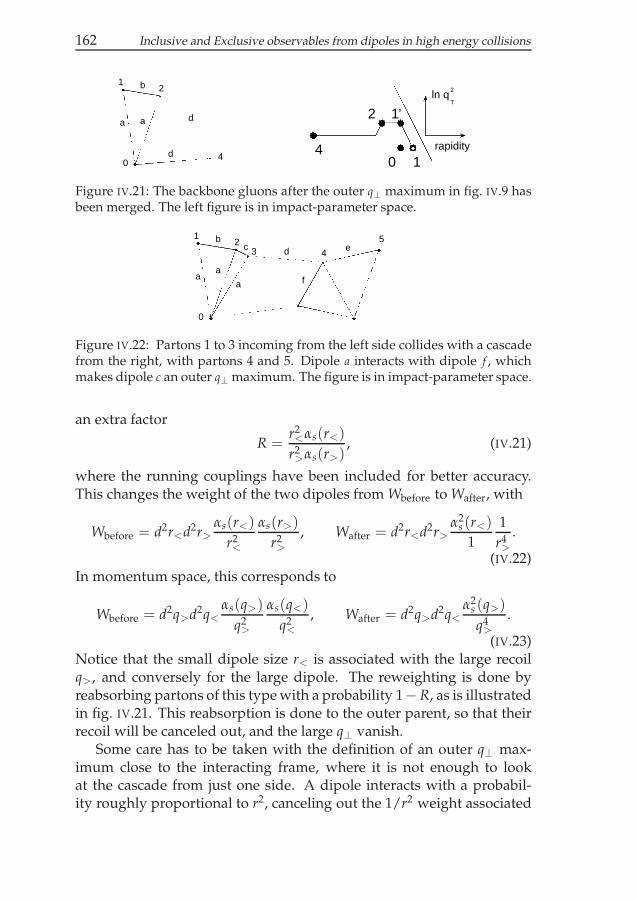
162 Inclusive and Exclusive observables from dipoles in high energy collisions
0
12
4
a
b
da
d0 1
1’2
4
ln q
rapidity
T
2
Figure IV.21: The backbone gluons after the outer q⊥ maximum in fig. IV.9 hasbeen merged. The left figure is in impact-parameter space.
0
12
3
a
bc
a
a
4
5d e
f
Figure IV.22: Partons 1 to 3 incoming from the left side collides with a cascadefrom the right, with partons 4 and 5. Dipole a interacts with dipole f , whichmakes dipole c an outer q⊥ maximum. The figure is in impact-parameter space.
an extra factor
R =r2<αs(r<)
r2>αs(r>)
, (IV.21)
where the running couplings have been included for better accuracy.This changes the weight of the two dipoles from Wbefore to Wafter, with
Wbefore = d2r<d2r>
αs(r<)
r2<
αs(r>)
r2>
, Wafter = d2r<d2r>
α2s (r<)
1
1
r4>
.
(IV.22)In momentum space, this corresponds to
Wbefore = d2q>d2q<
αs(q>)
q2>
αs(q<)
q2<
, Wafter = d2q>d2q<
α2s (q>)
q4>
.
(IV.23)Notice that the small dipole size r< is associated with the large recoilq>, and conversely for the large dipole. The reweighting is done byreabsorbing partons of this type with a probability 1−R, as is illustratedin fig. IV.21. This reabsorption is done to the outer parent, so that theirrecoil will be canceled out, and the large q⊥ vanish.
Some care has to be taken with the definition of an outer q⊥ max-imum close to the interacting frame, where it is not enough to lookat the cascade from just one side. A dipole interacts with a probabil-ity roughly proportional to r2, canceling out the 1/r2 weight associated

IV.B Absorbed partons and ordering 163
with its emission, and the colour flow will be recoupled over to the otherstate. Looking at fig. IV.22, parton 3 will not fit the above definition forouter q⊥, as it has no emissions on either side. However, since the dipoleon one side is interacting, and the dipole on the other side is not, dipolec will still be a q⊥ maximum with incorrect weight. The Monte Carlouses a generalized algorithm that covers also these cases, and uses thedipole d in fig. IV.22 as the larger dipole to reweight and possible reab-sorb parton 3.
Outer q⊥ maxima from the interaction, for example if d would besmallest dipole, does not have to be corrected as the interaction ampli-tude fij already has the correct weight for large q⊥.
This procedure ensures that the spectrum of large q⊥ from the cas-
cade and interaction is indeed going asd2q>α2
s (q>)
q4>
. The proportionality
constant is set from the known amplitude for a strictly increasing chainin q⊥, and the known “penalty” for being unordered.
This extra reweighting was not needed before, as only inclusive ob-servables were considered which are not affected by this procedure. Aninteracting dipole is always counted as an inner dipole in the final state,which means that no interacting dipole will be removed in this way, andthe inclusive interaction probability for the two cascades is unchanged.
IV.B Absorbed partons and ordering
1
1’
2
ln qT
2
rapidity
Figure IV.23: An emis-sion limits the orderedphase space of the par-ents.
In the previous sections, we describe how thebackbone gluons are controlled for orderingand reweighted, and some partons are ab-sorbed. An absorbed parton returns the q+ toits parents, and the transverse recoils are un-done. This will in general move the parentsback in rapidity and down in q⊥, which opensup a larger ordered phase space for the par-ents as in fig. IV.23. After parton 2 is emitted,taking part of the q+ from the parent and giv-ing a q⊥ recoil, 1’ is still allowed to continueemitting. For these emissions to be ordered inq+ and q−, they have to be between the dottedlines in fig. IV.23. If parton 2 was not emit-ted though, the larger order phase space be-tween the dashed lines would have been or-
IV

164 Inclusive and Exclusive observables from dipoles in high energy collisions
dered with respect to 1.
If the virtual cascade would only allow emissions ordered in q+ andq−, every absorbed gluon would open a part of phase space for emis-sions from the parents that has not been considered in the virtual cas-cade. This is solved by partially relaxing the ordering in the virtualcascade, and thus overestimating the ordered phase space to cover thecase of reabsorbed partons. Care has to be taken though, as the virtualcascade, before any reabsorbtions, will be used to calculate inclusiveobservables. As the backbone gluons are not yet decided when the cas-cade is made, it is from this approach not possible to use the correctordered phase space already for inclusive observables, and at the sametime cover all necessary phase space for all possible sets of backbonegluons.
However, by estimating what the backbone gluons may look likealready in the virtual cascade one can find a sufficiently good middleway: not too strict ordering so that an important part of the possiblefinal states get cut away, but not too open overestimate so that the in-clusive cross sections inflates.
IV.B.1 Coherence
Three observation at this point will all point towards the same solution:
• Only large q⊥ emissions, like the one in fig. IV.23, significantlychange the parents momenta. Thus it is only absorption of a stepup in q⊥ that risks shadowing emissions from the parent.
• The phase space that get shadowed mainly concerns small q⊥emissions. That is, the issue is when a large q⊥ parton is emit-ted and later absorbed, where the parent has not been allowed toemit with small q⊥.
• Many of the absorbed backbone gluons are absorbed due to anouter q⊥ maximum. This is exactly the scenario described in theprevious two points, that is an absorbed step up in q⊥ that shad-ows a step down in q⊥.
In DIPSY, when a dipole is emitted in the virtual cascade, it is not onlyemitted by the parton at the end of the dipole, but coherently by allpartons being close to the end of the dipole. This means that recoil andordering is using an effective parton with the summed momenta of allthe partons within range, where the range is set by the distance fromthe parent to the emitted gluon.

IV.B Absorbed partons and ordering 165
1
23
4
0
0 1
1’
2
2’3
3’4
ln q
rapidity
T
2
(a)
1
23
4
0
0 1
1’
2
2’3
4
ln q
rapidity
T
2
(b)
1
23
4
0
0 1
1’2
2’3
4
ln qT
2
rapidity
(c)
Figure IV.24: A parton emission (4), being emitted at different distances. Theupper figures are in impact-parameter space, and the lower figures are in y-q⊥representation, where the dotted lines show the limits of the q+ and q− order-ing. The circles in the upper figures show the coherence range of the emission.
This procedure is shown in fig. IV.24, where parton 4 is emitted at dif-ferent distances from its parent. In (a), the emission is a smaller dipolethan the previous one, and the coherence range is smaller than the dis-tance to the previous parton 2, so the recoil and ordering will be doneby parton 3 only. If the emission is at a larger distance than the previ-ous emission, as in (b), then the emission will be done by an effectiveparton with the merged momenta of parton 2 and 3. Notice that therecoil between 2 and 3 will cancel when their momenta are added, andthe effective parton will have the momentum of the original parton 2,as shown in the lower figure (b). Emissions at larger distance will con-tinue to add parton to the effective parton, and can allow emissions thatare not ordered with the parent itself, as in (c).
An outer q⊥ maximum is always a small dipole followed by a largerdipole, and reweighting will sometimes merge the two close by partonsto one. The extra ordered phase space opened by this merging is exactlythe part of phase space used by the coherent emissions at long distance,which can be seen by comparing figures IV.9, IV.21 and IV.24(b). This
IV

166 Inclusive and Exclusive observables from dipoles in high energy collisions
algorithm thus ensures that an absorbed outer q⊥ maximum can notopen up a part of phase space that was not considered in the virtualcascade. By solving this issue, we have been forced to introduce co-herence, where an emitted gluon cannot resolve partons that are closertogether than its wavelength.
While this increased ordered phase space will cover all situationsin the final state, some care has to be taken. First, some of the smalldipoles that emit coherently will not be absorbed, and in that case thevirtual cascade has emitted large dipoles in unordered regions. Theselarge dipoles have a significant effect on inclusive observables, and thetotal cross sections may get inflated.
Second, the large unordered dipoles are emitted with the motivationthat the previous small dipole may get emitted. However, the situationcan be that the small dipole will be absorbed because the large dipolewas emitted, as the large emission makes the previous small dipole aq⊥ maximum. Thus coherence is an estimate of how the final state willlook which is to some extent self-fulfilling.
With this in mind, full coherence as described above may need tobe scaled back to give a more accurate description. This was addressedin sec. IV.5.2 where frame independence was used in deciding exactlywhat phase space should should be considered as ordered in the virtualcascade.
IV.B.2 Ordering in the interaction
Like with the virtual cascade it is impossible to use an ordering thatallows the correct part of phase space for both inclusive and exclusiveobservables, but again some observations can be made.
1. The final result should not depend on whether a recoil comes fromthe cascade or the interaction. Thus the ordering in the interactionshould allow the same backbone gluons as the ordering in the cas-cade.
2. It is not possible to use the exact same ordering as in the virtualcascade, as the situation is fundamentally different. At a certainrapidity in the virtual cascade, the partons have not yet gottenrecoils from emissions at later rapidities. Thus, ordering in thevirtual cascade is checked when only recoils with partons in onedirection have been made. The same is not true in the interaction,where all recoils in both cascades are already made.
3. Events where an outer q⊥ maximum next to an interaction, as in
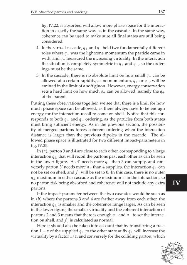
IV.B Absorbed partons and ordering 167
fig. IV.22, is absorbed will allow more phase space for the interac-tion in exactly the same way as in the cascade. In the same way,coherence can be used to make sure all final states are still beingconsidered.
4. In the virtual cascade, q+ and q− held two fundamentally differentroles where q+ was the lightcone momentum the particle came inwith, and q− measured the increasing virtuality. In the interactionthe situation is completely symmetric in q+ and q−, so the order-ings must be the same.
5. In the cascade, there is no absolute limit on how small q− can beallowed at a certain rapidity, as no momentum, q+ or q−, will beemitted in the limit of a soft gluon. However, energy conservationsets a hard limit on how much q+ can be allowed, namely the q+
of the parent.
Putting these observations together, we see that there is a limit for howmuch phase space can be allowed, as there always have to be enoughenergy for the interaction recoil to come on shell. Notice that this cor-responds to both q+ and q− ordering, as the particles from both statesmust bring sufficient energy. As in the previous section, the possibil-ity of merged partons forces coherent ordering when the interactiondistance is larger than the previous dipoles in the cascade. The al-lowed phase space is illustrated for two different impact-parameters infig. IV.25.
In (a), parton 3 and 4 are close to each other, corresponding to a largeinteraction q⊥ that will recoil the partons past each other as can be seenin the lower figure. As 4’ needs more q− than 3 can supply, and con-versely parton 3’ needs more q+ than 4 supplies, the interaction q⊥ cannot be set on shell, and fij will be set to 0. In this case, there is no outerq⊥ maximum in either cascade as the maximum is in the interaction, sono parton risk being absorbed and coherence will not include any extrapartons.
If the impact-parameter between the two cascades would be such asin (b) where the partons 3 and 4 are farther away from each other, theinteraction q⊥ is smaller and the coherence range larger. As can be seenin the lower figure, the smaller virtuality and the coherent interaction ofpartons 2 and 3 means that there is enough q+ and q− to set the interac-tion on shell, and fij is calculated as normal.
Here it should also be taken into account that by transferring a frac-tion 1 − z of the supplied q+ to the other state at fix q⊥ will increase thevirtuality by a factor 1/z, and conversely for the colliding parton, which
IV

168 Inclusive and Exclusive observables from dipoles in high energy collisions
0
12 3
4
5
a b
1
1’
2
2’
34
5
5’
4’ 3’ln q
rapidity
T
2
(a)
0
12 3
45
a
b
1
1’2
2’ 3
4 5
5’
4’
ln q
rapidity
T
2
(b)
Figure IV.25: Ordering in an interaction for two different impact-parameters,where parton 1-3 are belonging to one cascade, and 4 and 5 to the other. Theupper figures are in impact-parameter space, and the circles shows the coher-ence range in the interaction for parton 3 and 4. The lower figures are in y-q⊥representation, where vertical dashed line is the interaction frame y0, the hor-izontal full line marks the interaction q⊥, and the diagonal dotted lines marksthe q− and q+ parton 3 and 4 respectively brings to the interaction.
gives the limit for allowed interactions:
q+q− > 16q2⊥int, (IV.24)
where q+ and q− are the supplied lightcone momenta from the interact-ing effective partons, and q⊥int is the transverse recoil from the interac-tion.
This is a minimum for what has to be cut away in the ordering, andfrom frame independence it turns out that it can not be stricter (see sec-tion IV.5.1), thus motivating us to set the allowed phase space in fij toeq. eq. (IV.24) .
IV.C Saturation effects
All motivations and examples discussed above have been based on asingle backbone gluon chain, but in LHC events there will be severalchains branching of and merging due to multiple interactions and the

IV.C Saturation effects 169
swing. This complicates the situation for most of the arguments pre-sented previously in this section. However, the algorithms have beendesigned with saturation effects in mind, to give realistic results in allsituations. Here follows some of the larger effects from saturation, andhow the above algorithms handle them.
IV.C.1 Multiple interaction
1
0 2
3
4
5
6
7
8
Figure IV.26: Two interactions makesa chain split in two. Dotted linesshow parent structure, full lines showcolour flow. The picture is in impact-parameter space.
In the interaction, multiple scat-terings are allowed, which meansthat there will be several chainscutting the interaction frame.These chains will merge at somepoint when following them back,if not before, they will alwaysmeet at the valence partons. Thisdoes not introduce any compli-cations for the ordering. Eachemission is controlled at the timeof the emission, and if anotherbranch has taken energy from theparents, then the ordered phasespace for emission will be smaller,which is expected.
One has to be a bit careful with the reweighting however, but thealgorithm described in sec. IV.4.3 is made to handle both splitting andmerging chains. The dipoles created with a weight of d2r/r2 are still thepartons that have on-shell children on one side, but not on the other,and therefore the definition of an outer q⊥ maximum can remain.
This is illustrated in fig. IV.26, where a backbone chain splits upin two due to multiple interaction. Dipoles (24) and (34) both get theweight d2r corresponding to d2q⊥/q4
⊥, and they will get two factors ofαs(r) in case of q⊥ maximum. Thus they do not need any extra suppres-sion, and they do indeed not fit the definition of outer dipole, as parton4 has children on both sides. For all other partons and dipoles, the argu-ments for the single chain can be applied as normal, so the reweightingalgorithm works also with multiple interactions.
IV.C.2 The Swing
IV

170 Inclusive and Exclusive observables from dipoles in high energy collisions
0
1
2
3
4
5
6
78
9
Figure IV.27: A swing between (45)and (26) causing two chains of back-bone gluons to merge. Dotted linesshow parent structure, full lines showcolour flow. The picture is in impact-parameter space.
The dipole swing in the virtualcascade does not cause any re-coils, but it does affect the par-ent structure of future emissions.In a non-swinged, single interac-tion chain, one of the two parentsof each parton will also be parentto the other parent, making forthe typical ladder-like structureseen in previous figures. How-ever, with swinged emissions thisis no longer true, and the two par-ents can have 4 different parents.
This is seen in fig. IV.27 wherea swing has recoupled dipole (45)and (26) into (24) and (56), (56)then evolves further and inter-acts, while (24) does not interact.Here the parents of parton 8 and 9 cover all the partons (notice that theparents of 7 are parton 5 and 6), so all partons are set on-shell. Notice inthe figure that even though parton 4 is colour connected to 2 from theswing, parton 4 was not emitted by 2 (it was emitted by 0 and 1); thusno recoil has been made between the two partons, and no reweightinghas to be made.
Dipole (14) has the weight 1/r2 from the cascade and is an outerdipole as parton 4 has no children on that side. Thus (14) will, if smallerthan (45), be reweighted by
r214αs(r14)
r245αs(r45)
(IV.25)
from eq. eq. (IV.21) , and reweighting again produces the correctweights. Correspondingly for parton 2, which is in the same situation as4, but since 2 is a valence parton with no parents, there is no reweight-ing to be done. Dipole (45) is not an outer dipole because parton 7 is achild of 5 on the same side as (45), so no reweighting will be done. If(45) is a q⊥ maximum, it will be emitted with a weight α(r45)/r2
45, and
the swing is made with a probabilityr2
45r226
r224r2
56, giving the weight
r045α(r45) ↔ α(r45)
q445⊥
. (IV.26)

IV.C Saturation effects 171
Notice that while the power of q⊥ is the correct one, a power in therunning coupling is missing. This power of αs will instead come fromthe smallest dipole in the emission of parton 7 from 5 and 6. Thus, asaturated cascade can give rise to q⊥ maxima where one of the powersin αs is at the wrong scale.
This flaw can possibly be mended by introducing a running αs inthe swing amplitude, but in the current version of DIPSY it is not imple-mented. As it is a next to leading order factor in the weight occurringonly in special configurations of a saturated cascade, it is estimated tobe a small effect.
In conclusion, the algorithm in section IV.4.3 will still provide a sat-isfactory treatment of reweighting outer q⊥ maxima.
IV.C.3 colour flow in saturated cascades
For a saturated cascade, the colour flow does not necessarily return tothe original structure when the virtual emissions are removed accordingto IV.4.5. The swings are changing the colour structure, and after all thevirtual emissions are reabsorbed, the colour flow does not necessarilyreproduce the structure without the virtual emissions. An example ofsuch a virtual cascade and backbone gluons is shown in fig. IV.28.
Swings where one of the swinged dipoles go on to interact willmerge two backbone chains, as was seen in sec. IV.3.2, and are veryimportant for a frame-independent description. Swings by an outerdipole, such as A, will not influence the choice of backbone gluons, butcan reconnect the colour flow between the backbone gluons. A colourreconnection between backbone gluons can also happen by a swing be-tween virtual dipoles, if the dipoles originate from different parts of thebackbone chain, as is the case for swing C. If the two swinging virtualdipoles originate from the same part on the backbone chain, as swingD, no difference will be seen in the colour flow between the backbonegluons.
In this way, not only exchange of individual soft gluons betweenthe chains are simulated, but virtual chains of soft and hard gluons cancarry colour flow between the chains, or between different parts of thesame chain. The virtual cascade can thus give a very dynamic and de-tailed description on how the colour flow changes in saturated environ-ments, which will be increasingly important at high energies, and canbe an essential ingredient in heavy ion collisions.
IV

172 Inclusive and Exclusive observables from dipoles in high energy collisions
A
B
C
D
r
rapidityr
rapidity
Figure IV.28: A cascade with swings and multiple interactions. The longdashed lines on the left side are the three valence dipoles of a proton. Fulllines mark colour flow and dotted lines mark emissions. There are three inter-actions, which are the colour lines passing over the interaction rapidity markedby a vertical dashed line to the right. The big dots are the backbone gluons, se-lected through tracing each interaction back towards the valence partons, andthe rest of the partons are virtual. The left figure is the virtual cascade, andfour swings A to D are highlighted with thick lines. The right figure shows thebackbone gluons after the virtual partons have been absorbed.

IV References 173
IV References
[1] E. A. Kuraev, L. N. Lipatov, and V. S. Fadin, “The PomeranchukSingularity in Nonabelian Gauge Theories,” Sov. Phys. JETP 45
(1977) 199–204.
[2] I. I. Balitsky and L. N. Lipatov, “The Pomeranchuk Singularity inQuantum Chromodynamics,” Sov. J. Nucl. Phys. 28 (1978) 822–829.
[3] E. Avsar, G. Gustafson, and L. Lonnblad, “Energy conservationand saturation in small-x evolution,” JHEP 07 (2005) 062,arXiv:hep-ph/0503181.
[4] E. Avsar, G. Gustafson, and L. Lonnblad, “Small-x dipoleevolution beyond the large-N(c) limit,” JHEP 01 (2007) 012,arXiv:hep-ph/0610157.
[5] E. Avsar, G. Gustafson, and L. Lonnblad, “Difractive Excitation inDIS and pp Collisions,” JHEP 12 (2007) 012, arXiv:0709.1368[hep-ph].
[6] C. Flensburg, G. Gustafson, and L. Lonnblad, “Elastic andquasi-elastic pp and γ∗p scattering in the Dipole Model,” Eur.Phys. J. C60 (2009) 233–247, arXiv:0807.0325 [hep-ph].
[7] C. Flensburg and G. Gustafson, “Fluctuations, Saturation, andDiffractive Excitation in High Energy Collisions,” JHEP 10 (2010)014, arXiv:1004.5502 [hep-ph].
[8] A. H. Mueller, “Soft gluons in the infinite momentum wavefunction and the BFKL pomeron,” Nucl. Phys. B415 (1994) 373–385.
[9] A. H. Mueller and B. Patel, “Single and double BFKL pomeronexchange and a dipole picture of high-energy hard processes,”Nucl. Phys. B425 (1994) 471–488, hep-ph/9403256.
[10] A. H. Mueller, “Unitarity and the BFKL pomeron,” Nucl. Phys.B437 (1995) 107–126, hep-ph/9408245.
[11] E. Iancu, A. Leonidov, and L. McLerran, “The Color glasscondensate: An Introduction,” arXiv:hep-ph/0202270 [hep-ph].
[12] E. Iancu and R. Venugopalan, “The Color glass condensate andhigh-energy scattering in QCD,” arXiv:hep-ph/0303204
IV

174 Inclusive and Exclusive observables from dipoles in high energy collisions
[hep-ph]. To be published in QGP3, Eds. R.C. Hwa andX.N.Wang, World Scientific.
[13] F. Gelis, E. Iancu, J. Jalilian-Marian, and R. Venugopalan, “TheColor Glass Condensate,” arXiv:1002.0333 [hep-ph]. *Temporary entry *.
[14] E. Iancu, A. Leonidov, and L. D. McLerran, “Nonlinear gluonevolution in the color glass condensate. 1.,” Nucl.Phys. A692 (2001)583–645, arXiv:hep-ph/0011241 [hep-ph].
[15] J. Jalilian-Marian, A. Kovner, A. Leonidov, and H. Weigert, “TheBFKL equation from the Wilson renormalization group,”Nucl.Phys. B504 (1997) 415–431, arXiv:hep-ph/9701284[hep-ph].
[16] S. Catani, F. Fiorani, and G. Marchesini, “Small x Behavior ofInitial State Radiation in Perturbative QCD,” Nucl. Phys. B336
(1990) 18.
[17] M. Ciafaloni, “Coherence Effects in Initial Jets at Small q**2 / s,”Nucl. Phys. B296 (1988) 49.
[18] B. Andersson, G. Gustafson, and J. Samuelsson, “The Linkeddipole chain model for DIS,” Nucl. Phys. B467 (1996) 443–478.
[19] G. P. Salam, “Soft emissions and the equivalence of BFKL andCCFM final states,” JHEP 03 (1999) 009, hep-ph/9902324.
[20] M. L. Good and W. D. Walker, “Diffraction disssociation of beamparticles,” Phys. Rev. 120 (1960) 1857–1860.
[21] G. P. Salam, “An introduction to leading and next-to-leadingBFKL,” Acta Phys. Polon. B30 (1999) 3679–3705, hep-ph/9910492.
[22] A. H. Mueller and G. P. Salam, “Large multiplicity fluctuationsand saturation effects in onium collisions,” Nucl. Phys. B475 (1996)293–320, hep-ph/9605302.
[23] J. Kwiecinski, A. D. Martin, and P. J. Sutton, “Constraints on gluonevolution at small x,” Z. Phys. C71 (1996) 585–594,hep-ph/9602320.
[24] I. Balitsky and G. A. Chirilli, “NLO evolution of color dipole,”Acta Phys. Polon. B39 (2008) 2561–2566.

IV References 175
[25] E. Avsar, “On the High Energy Behaviour of The Total CrossSection in the QCD Dipole Model,” JHEP 04 (2008) 033,arXiv:0803.0446 [hep-ph].
[26] V. N. Gribov and L. N. Lipatov, “Deep inelastic e p scattering inperturbation theory,” Yad. Fiz. 15 (1972) 781–807.
[27] Y. L. Dokshitzer, “Calculation of the structure functions for deepinelastic scattering and e+e− annihilation by perturbation theoryin quantum chromodynamics. (In Russian),” Sov. Phys. JETP 46
(1977) 641–653.
[28] G. Altarelli and G. Parisi, “Asymptotic freedom in partonlanguage,” Nucl. Phys. B126 (1977) 298.
[29] H. Kharraziha and L. Lonnblad, “The linked dipole chain MonteCarlo,” JHEP 03 (1998) 006, hep-ph/9709424.
[30] H. Kharraziha and L. Lonnblad, “LDCMC version 1.0,” Comput.Phys. Commun. 123 (1999) 153.
[31] G. Gustafson, “Dual description of a confined color field,”Phys. Lett. B175 (1986) 453.
[32] G. Gustafson and U. Pettersson, “Dipole Formulation of QCDCascades,” Nucl. Phys. B306 (1988) 746.
[33] L. Lonnblad, “ARIADNE version 4: A Program for simulation ofQCD cascades implementing the color dipole model,”Comput. Phys. Commun. 71 (1992) 15–31.
[34] B. Andersson, G. Gustafson, and B. Soderberg, “A GENERALMODEL FOR JET FRAGMENTATION,” Z. Phys. C20 (1983) 317.
[35] B. Andersson, G. Gustafson, G. Ingelman, and T. Sjostrand,“Parton fragmentation and string dyanmics,” Phys. Rept. 97 (1983)31.
[36] T. Sjostrand, S. Mrenna, and P. Z. Skands, “A Brief Introduction toPYTHIA 8.1,” Comput. Phys. Commun. 178 (2008) 852–867,arXiv:0710.3820 [hep-ph].
[37] T. Sjostrand, S. Mrenna, and P. Z. Skands, “PYTHIA 6.4 Physicsand Manual,” JHEP 05 (2006) 026, arXiv:hep-ph/0603175.
IV

176 Inclusive and Exclusive observables from dipoles in high energy collisions
[38] UA4 Collaboration, D. Bernard et al., “LARGE t ELASTICSCATTERING AT THE CERN SPS COLLIDER AT S**(1/2) =630-GeV,” Phys. Lett. B171 (1986) 142.
[39] NA22 Collaboration, M. Adamus et al., “STUDY OF ELASTIC pi+p, K+ p AND p p SCATTERING AT 250- GeV/c,” Phys. Lett. B186
(1987) 223–226.
[40] CDF Collaboration, F. Abe et al., “Measurement of small angle ppelastic scattering at
√s = 546 GeV and 1800 GeV,” Phys. Rev. D50
(1994) 5518–5534.
[41] CDF Collaboration, F. Abe et al., “Measurement of the pp totalcross-section at
√s = 546 GeV and 1800-GeV,” Phys. Rev. D50
(1994) 5550–5561.
[42] E-710 Collaboration, N. A. Amos et al., “A LUMINOSITYINDEPENDENT MEASUREMENT OF THE anti-p p TOTALCROSS-SECTION AT S**(1/2) = 1.8-TeV,” Phys. Lett. B243 (1990)158–164.
[43] E-710 Collaboration, N. A. Amos et al., “Anti-proton - protonelastic scattering at s**(1/2) = 1.8- TeV from |t| = 0.034-GeV/c**2to 0.65-GeV/c**2,” Phys. Lett. B247 (1990) 127–130.
[44] E-811 Collaboration, C. Avila et al., “The ratio, rho, of the real tothe imaginary part of the anti-p p forward elastic scatteringamplitude at s**(1/2) = 1.8-TeV,” Phys. Lett. B537 (2002) 41–44.
[45] UA4/2 Collaboration, C. Augier et al., “Measurement of the proton- anti-proton total cross- section at the S anti-p p S collider by aluminosity dependent method,” Phys. Lett. B344 (1995) 451–454.
[46] M. M. Block, F. Halzen, and T. Stanev, “Extending the frontiers:Reconciling accelerator and cosmic ray p p cross sections,” Phys.Rev. D62 (2000) 077501, arXiv:hep-ph/0004232.
[47] ZEUS Collaboration, S. Chekanov et al., “Study of deep inelasticinclusive and diffractive scattering with the ZEUS forward plugcalorimeter,” Nucl. Phys. B713 (2005) 3–80, hep-ex/0501060.
[48] H1 Collaboration, A. Aktas et al., “Measurement of deeply virtualCompton scattering at HERA,” Eur. Phys. J. C44 (2005) 1–11,arXiv:hep-ex/0505061.

IV References 177
[49] H1 Collaboration, F. D. Aaron et al., “Measurement of DeeplyVirtual Compton Scattering and its t-dependence at HERA,” Phys.Lett. B659 (2008) 796–806, arXiv:0709.4114 [hep-ex].
[50] L. Lonnblad, “ThePEG, Pythia7, herwig++ and Ariadne,”Nucl.Instrum.Meth. A559 (2006) 246–248.
[51] M. Bahr et al., “Herwig++ Physics and Manual,” Eur. Phys. J. C58
(2008) 639–707, arXiv:0803.0883 [hep-ph].
[52] A. Buckley et al., “Rivet user manual,” arXiv:1003.0694
[hep-ph].
[53] Atlas Collaboration Collaboration, G. Aad et al., “Measurement ofunderlying event characteristics using charged particles in ppcollisions at
√s = 900GeV and 7 TeV with the ATLAS detector,”
arXiv:1012.0791 [hep-ex]. * Temporary entry *.
[54] ATLAS Collaboration Collaboration, G. Aad et al.,“Charged-particle multiplicities in pp interactions measured withthe ATLAS detector at the LHC,” New J.Phys. (2010) ,arXiv:1012.5104 [hep-ex]. Long author list - awaitingprocessing.
[55] CDF Collaboration, A. A. Affolder et al., “Charged jet evolutionand the underlying event in pp collisions at 1.8 TeV,” Phys. Rev.D65 (2002) 092002.
[56] A. Buckley, J. Butterworth, S. Gieseke, D. Grellscheid, S. Hoche, etal., “General-purpose event generators for LHC physics,”arXiv:1101.2599 [hep-ph].
[57] R. Corke and T. Sjostrand, “Interleaved Parton Showers andTuning Prospects,” arXiv:1011.1759 [hep-ph].
[58] CDF Collaboration, R. Field, “Min-bias and the underlying eventin Run 2 at CDF,” Acta Phys. Polon. B36 (2005) 167–178.
[59] C. Flensburg, G. Gustafson, L. Lonnblad, and A. Ster,“Correlations in double parton distributions at small x,”arXiv:1103.4320 [hep-ph].
IV