A discrete choice model for large heterogeneous panels with interactive fixed effects with an application to the determinants of corporate bond issuance

Lena BonevaOliver Linton

The Institute for Fiscal Studies Department of Economics, UCL

cemmap working paper CWP02/17

A Discrete Choice Model For Large Heterogeneous

Panels with Interactive Fixed Effects with an

Application to the Determinants of Corporate Bond

Issuance∗

Lena Boneva†

Bank of England and CEPR

Oliver Linton‡

University of Cambridge

January 3, 2017

Abstract

What is the effect of funding costs on the conditional probability of issuinga corporate bond? We study this question in a novel dataset covering 5610issuances by US firms over the period from 1990 to 2014. Identification of thiseffect is complicated because of unobserved, common shocks such as the globalfinancial crisis. To account for these shocks, we extend the common correlatedeffects estimator to settings where outcomes are discrete. Both the asymptoticproperties and the small sample behavior of this estimator are documented. Wefind that for non-financial firms, yields are negatively related to bond issuancebut that effect is larger in the pre-crisis period.

Keywords: Heterogeneous panel data; discrete choice models; capital struc-tureJEL classification: C23; C25; G32

∗We would like to thank Peter Robinson, our editor Thierry Magnac and 3 anonymous refereesfor their helpful comments and Hashem Pesaran, Martin Weidner, Lu Liu, Menno Middeldorp andMagda Rutkowska for many useful discussions. The views expressed in this paper are those ofthe authors and do not necessarily reflect the views of the Bank of England, the Monetary PolicyCommittee, the Financial Policy Committee or the Prudential Regulation Authority.†Bank of England, Threadneedle St, London, EC2R 8AH. Email:

Lena.Boneva@bankofengland.co.uk. Financial support from Cusanuswerk and the ESRC(grant no.: K67783X) is gratefully acknowledged.‡Faculty of Economics, Austin Robinson Building, Sidgwick Avenue, Cambridge, CB3 9DD.

Email: obl20@cam.ac.uk. Financial support from the Keynes Fund is gratefully acknowledged.

1

1 Introduction

At least since Modigliani and Miller (1958), how firms choose their capital structure

has attracted much attention and there is a large empirical and theoretical literature

that explores these issues (e.g. Myers (1977), Myers and Majluf (1984), Denis and

Mihov (2003), Becker and Ivashina (2014)). Relative to other forms of financing such

as equity and bank loans, corporate debt is an important source of funding for US

corporations (Denis and Mihov (2003)) and the corporate bond market has grown

rapidly over the last decade (Office of Financial Research (2015)).

In this paper, we study the effect of corporate yields on bond issuance of US firms.

In contrast to earlier studies (e.g. Frank and Goyal (2008)), we adopt an incremental

approach that investigates the conditional probability of issuing a corporate bond

which is particularly suitable for questions related to time-variation in the regressors.

While previous work has documented that issuer characteristics like size, rating,

profitability, leverage, equity prices, monetary policy, information asymmetry and

the supply of bank credit are important determinants of bond issuance (e.g. Mizen

and Tsoukas (2013), Badoer and James (2016), Adrian et al. (2012), Denis and Mihov

(2003), Becker and Ivashina (2014), Gomes and Phillips (2012)), there is not much

evidence yet on the effect of yields on bond issuance.

Answering the question of how funding costs in corporate bond markets affect

issuance decisions sheds light on a particular transmission mechanism of monetary

policy: by means of conventional and unconventional monetary policy tools, the

central bank can affect the interest rates firms face in corporate bond markets. Bond

issuance, on the other hand, tends to be related to corporate investment and thus

aggregate demand (Farrant et al. (2013)).

We study the effect of yields on bond issuance using a novel dataset that includes

bond issuances by US firms between 1990 and 2015 on a monthly frequency. During

that period, we observe 5610 issuances with an average size of approximately 300

million USD made by 1004 different firms. We find that for non-financial firms,

yields are negatively related to bond issuance but that effect is larger in the pre-crisis

period. In contrast, there is no significant effect of yields on corporate bond issuance

2

for financial firms. Splitting the data by the credit rating of the issuer reveals that

the negative relationship between yields and corporate bond issuance is driven by

firms with a low credit rating. These results are robust to applying different sample

selection criteria, to including additional regressors and to using corporate spreads

instead of yields as the primary regressor.

To identify the parameters of interest, it is important to control for unobserved,

common shocks that are frequently encountered in these type of datasets. In our em-

pirical application, the unobserved factors can represent a new regulatory landscape,

changes in investor behavior such as search for yield, automated trading or policies

that aim at deepening corporate bond markets, for example. Andrews (2005) shows

that common shocks create problems for inference if data are available for a single

cross-sectional unit and the model is estimated by least squares or instrumental vari-

able methods. But the increased availability of panel data where both the time series

and cross-sectional dimensions are large offers new opportunities for controlling for

these unobserved shocks. Bai (2009) and Pesaran (2006) are examples for panel data

estimators robust to common shocks.

This paper contributes to this literature by developing an estimator for large

heterogeneous panels with cross-sectional dependence in a framework where outcomes

are discrete. The proposed estimator belongs to the class of common correlated

effects (CCE) estimators that approximate the unobserved factors with cross-sectional

averages of both the regressors and the response variable (Pesaran (2006)). But this

approach is complicated in nonlinear models where it is difficult to use averages of

response variables without making strong assumptions. This paper adopts the CCE

estimation methodology to discrete choice models under the assumption that the

unobserved factors are contained in the span of the observed factors and the cross-

sectional averages of the regressors.

We present large sample distribution theory for our estimation procedures for

the setting where both the time dimension T and the cross-sectional dimension N

are large. We first show that the estimator of the individual-specific coefficients is

consistent and asymptotically normal. An important part of the asymptotic theory is

3

uniform consistency of the preliminary estimator, which we establish under moment

conditions. Based on the asymptotic properties of the estimators of the individual-

specific coefficients, we derive the consistency and asymptotic normality for the mean

group estimator that is defined as the average of the individual-specific estimators.

Inference regarding the mean group effect follows straightforwardly: we show that the

asymptotic variance of the mean group estimator can be estimated by the covariance

matrix of the individual-specific coefficient estimates. This covariance estimator is

similar to the estimator obtained in linear regression models (Pesaran (2006)).

By means of a simulation study, we document that for a wide range of factor

structures, the mean group estimator is comparable in terms of RMSE and bias to

an infeasible estimator that counterfactually assumes that the common factors are

known. In addition, the mean group estimator has good empirical power, size and

coverage probabilities.

Our paper is related to Fernandez-Val and Weidner (2016) and Chen et al. (2014)

who propose alternative estimators for large, nonlinear panels with fixed effects.

Fernandez-Val and Weidner (2016) study nonlinear panel data models with additive

fixed effects. They characterize the bias that arises due to the incidental parameter

problem (Neyman and Scott (1948)) and provide analytical and jackknife corrections

to remove this bias. In contrast to this paper, they assume that the slope coefficients

are homogeneous and that the fixed effects enter additively. Chen et al. (2014) is

probably the paper closest to ours. They also propose an estimator for nonlinear

panel data models with interactive fixed effects. But while the contribution we make

is along the lines of simplicity and applicability and indeed the application, their fo-

cus is on developing a comprehensive asymptotic theory for a wide range of nonlinear

panel data models. In contrast, we are only concerned with binary choice models

which are popular among applied economists. One advantage of our approach is

that our estimator can be computed by simply averaging regression coefficients from

Probit models estimated for each individual unit. In contrast, Chen et al. (2014)’s es-

timator is computed iteratively in a two-step procedure which makes it more difficult

to implement in practice.

4

Our paper is also related to the literature on common correlated effects estimation.

That literature was pioneered by Pesaran (2006) who first proposed to approximate

the unobserved factors by cross-sectional averages. Since then, a growing literature

has extended the CCE approach in various ways: Pesaran and Tosetti (2011) combine

the factor approach with spatial models by assuming that the disturbances net of the

common factors follow a spatial process, see also Chudik et al. (2011). Kapetanios

et al. (2011) show that the CCE estimator is consistent even if the unobserved factors

are non-stationary. Chudik and Pesaran (2015) extend the CCE estimator to dynamic

panels. Baltagi et al. (2015) develop a CCE estimator for data with structural breaks.

Harding and Lamarche (2014) propose a quantile CCE estimator for homogeneous

panel data with endogenous regressors, and Boneva et al. (2016) develop a quantile

CCE estimator for heterogeneous panels. The contribution of this paper is to extend

the CCE approach to discrete outcomes.

The remainder of this paper is organized as follows. The econometric model is

presented in Section 2 and Section 3 describes the estimation methodology and dis-

cusses related estimators for nonlinear panel data. Section 4 develops the asymptotic

theory. Section 5 reports the results of a simulation study and Section 6 applies

our estimator to investigate how yields affect the decision to issue a corporate bond.

Section 7 concludes.

2 Econometric model

This section describes the econometric framework. We observe a sample of panel

data (Yit, Xit, dt) : i = 1, . . . , N, t = 1, . . . , T, where i denotes the i-th unit and t

is the time point of observation. To keep the notation simple, we assume that the

panel is balanced. The data are assumed to come from the model

Y ∗it = αᵀ

i dt + βᵀ

iXit + eit, i = 1, . . . , N, t = 1, . . . , T, (1)

where Xit is a Kx × 1 vector of individual-specific regressors that are assumed to

be strictly exogenous and stationary and dt is a Kd × 1 vector of observed common

5

factors that do not vary across individual units. Here, Y ∗it is a latent variable that is

related to the observed response variable Yit via the indicator function I(.),

Yit = I(Y ∗it ). (2)

That is, Yit is unity if Y ∗it > 0 and zero otherwise. This paper is concerned with

inference for the heterogeneous coefficients βi and their mean. This is complicated

by cross-sectional dependence which is modeled by assuming that the disturbances

exhibit the factor structure

eit = κᵀ

i ft + εit, (3)

where ft is a Kf ×1 vector of unobserved common factors and κi is a Kf ×1 vector of

factor loadings. The disturbances εit are i.i.d. conditional on the factors and have a

known symmetric density φ and distribution function Φ (perhaps but not necessarily

the normal distribution with zero mean and unit variance). We may write

Pr(Yit = 1|Xit, dt, ft) = 1−Φ(−αᵀ

i dt − βᵀ

iXit − κᵀ

i ft) = Φ(αᵀ

i dt + βᵀ

iXit + κᵀ

i ft). (4)

In many panel data applications, the unobserved common factors ft are correlated

with both the response variable and the regressors, introducing a certain type of en-

dogeneity. To allow for this possibility, the individual-specific regressors are assumed

to follow the model

Xit = Aᵀ

i dt +Kᵀ

i ft + uit, (5)

where Ai is a coefficient matrix of dimension Kd ×Kx, and Ki is a Kf ×Kx matrix

of factor loadings and uit have a zero mean and are i.i.d. conditional on the common

factors.

We make the following assumptions, which are maintained throughout the paper:

(A1) Random coefficient model : the coefficients ϑi = (αᵀ

i , βᵀ

i , κᵀ

i , vec(Ai)ᵀ, vec(Ki)

ᵀ)ᵀ

are generated byϑi = ϑ0 + ηi, (6)

where ηi ∼i.i.d.(0,Σ) and is distributed independently of κj, Kj, εjt, ujt, dt, ftfor all i, j, t, ‖β‖ ≤ C <∞.

6

(A2) Common factors : the (Kf + Kd) × 1 vector of common factors gt = (fᵀ

t , dᵀ

t )ᵀ

is assumed to be bounded and covariance stationary with absolute summablecovariances, and distributed independently of the disturbances εit and uis, forall i, t, s.

(A3) Factor loadings : the factor loadings κi and Ki are i.i.d. across i, and distributedindependently of the disturbances εjt and ujt and the common factors ft anddt, for all i, j, t with finite means and variances.

(A4) The function Φ is three times differentiable.

3 Estimation

3.1 A common correlated effects estimator for discrete choice

panels

The econometric model (1)-(5) depends on the unobserved factors ft which makes

estimation difficult. One approach to control for unobserved factors is to approx-

imate them by cross-sectional averages of the regressors and the response variable

(Pesaran (2006)). But in nonlinear panel data models, it is difficult to use averages

of response variables without making strong assumptions. Instead, we approximate

the unobserved factors by cross-sectional averages of the regressors. This approach

is valid if the unobserved factors are contained in the span of the observed factors

and the cross-sectional averages of the regressors. This assumption is more restrictive

compared to the linear set-up in Pesaran (2006) where also the dependent variable

can be used to approximate the unobserved factors.1

Let h0t = A0ᵀdt + K0

ᵀft and ht = A

ᵀ

dt + Kᵀ

ft be vectors in RKx , where we use

A0 and K0 to denote the population means of Ai and Ki and A = N−1∑N

i=1Ai and

K = N−1∑N

i=1Ki to denote their sample counterparts. These quantities will be used

to rewrite the likelihood function. Then, under the assumption that for large N the

Kf ×Kx matrix K is of full rank:

rank(K) = Kf ≤ Kx, (7)

1In case of microeconometric panels where individual-specific unobserved characteristics like abil-ity are likely to be correlated with the regressors, the indices t and i can be interchanged andtime-series averages can be used to approximate the unobserved loadings.

7

we have ft = (K Kᵀ

)−1K ht − (KKᵀ)−1KA

ᵀ

dt. We also have for all t, N

Pr(Yit = 1|dt, Xit, ft) = Pr(Yit = 1|dt, Xit, ht) = Φ(αᵀ

i dt + βᵀ

iXit + κᵀ

iht), (8)

where αi = αi + Kᵀκi and κi = K

ᵀκi with K = (K K

ᵀ

)−1K . The true individual-

specific coefficients and their population means are denoted by θ0i = (αᵀ

0i, βᵀ

0i, κᵀ

0i)ᵀ,

θ0 = (αᵀ

0, βᵀ

0 , κᵀ

0)ᵀ ∈ RKd+2Kx .

Letting p denote the generic conditional distribution, we may define the infeasible

objective function

QiT (θ) =

1

T

T∑t=1

qit(θ, ht) (9)

= − 1

T

T∑t=1

log p(Yit|dt, Xit, ht, θ), (10)

= − 1

T

T∑t=1

[Yit log Φ(θᵀzit) + (1− Yit) log(1− Φ(θ

ᵀzit))],

where zit = (dᵀ

t , Xᵀ

it, hᵀ

t )ᵀ

and θ ∈ RKd+2Kx ; this requires knowledge of ht. Let θi =

(˜αᵀ

i , βᵀ

i , ˜κᵀ

i )ᵀ ∈ RKd+2Kx be defined as the (infeasible) minimizer of Qi

T (θ) with respect

to θ ∈ Θ. The quantity ht is no more observable than ft, but it has a direct analogue

or approximator, X t = N−1∑N

i=1 Xit. Define the Kx × 1 vector ht ≡ X t = Aᵀ

dt +

Kᵀ

ft+ut, where we switch notation to emphasize the connection with ht and h0t and

to understand ht as a large dimensional nuisance parameter that is replaced by the

sample quantity ht. Then define the feasible objective function

QiT (θ) =

1

T

T∑t=1

qit(θ, ht)

= − 1

T

T∑t=1

log p(Yit|dt, Xit, ht, θ) (11)

= − 1

T

T∑t=1

[Yit log Φ(θᵀzit) + (1− Yit) log(1− Φ(θ

ᵀzit))],

where zit = zit = (dᵀ

t , Xᵀ

it, hᵀ

t )ᵀ. The estimator θi = (αᵀ

i , βᵀ

i , κᵀ

i )ᵀ ∈ RKd+2Kx is defined

as the minimizer of QiT (θ) with respect to θ ∈ Θ. In practice, standard numerical al-

8

gorithms can be used to find the optimum, since after substituting for ht this amounts

to estimation of a parametric binary choice model with a known link function.

The mean group estimator is defined as

θ =1

N

N∑i=1

θi. (12)

We will have special interest in the subvector β. Define also the infeasible mean group

estimator θ =N∑i=1

θi/N.

3.2 Comparison with related estimators for nonlinear panels

This section compares our methodology to alternative estimators for large, nonlinear

panels with fixed effects (Fernandez-Val and Weidner (2016), Charbonneau (2014),

Sun (2016), Chen et al. (2014)).

Fernandez-Val and Weidner (2016) study nonlinear panel data models with indi-

vidual and time fixed effects. Compared to our paper, they assume that the fixed

effects enter the model additively and that the slope coefficients are homogeneous. So

their model can be obtained as a special case of the model (1)-(3) if βi = β, κi = κ and

dt = 1. While the assumption of slope homogeneity is probably too strong in many

applications it has the advantage that faster convergence rates can be obtained. The

contribution of Fernandez-Val and Weidner (2016) is to characterize the bias that

arises due to the incidental parameter problem (Neyman and Scott (1948)) and to

provide analytical and jackknife bias corrections.

Charbonneau (2014) and Sun (2016) also study nonlinear panel data models with

additive fixed effects and homogeneous slopes. Charbonneau (2014) develops a con-

ditional maximum likelihood approach to estimate discrete choice panel data models

with fixed effects which is analogous to the difference-in-differences estimator used

in linear panel data models. Sun (2016)’s estimator is obtained by maximizing a

modified objective function that is not affected by the incidental parameter problem.

Finally, Chen et al. (2014) is probably the paper closest to ours.2 They also

2A related paper is Chen (2014).

9

propose an estimator for nonlinear panel data models with interactive fixed effects.

But while the contribution we make is along the lines of simplicity and applicability

and indeed the application, their focus is on developing a comprehensive asymptotic

theory for a wide range of nonlinear panel data models. In particular, they provide

analytical and jackknife corrections for panel data models with interactive fixed effects

to eliminate the incidental parameter bias. From a practitioner’s point of view, ease of

implementation is one advantage of our approach: our estimator is obtained by simply

averaging regression coefficients from probit models estimated for each individual unit

while Chen et al. (2014)’s estimator is computed iteratively in a two-step procedure.

Another important difference to our paper is that Chen et al. (2014) assume that the

slope coefficients are homogeneous so their model is nested in the model (1)-(3) if

βi = β and dt = 1.

4 Asymptotic theory

This section characterizes the large sample properties of both the estimators of the

individual-specific coefficients and the mean group estimator in discrete choice panels

with interactive fixed effects.

Notation: We stack ht, ht, and h0t to form the TKx × 1 vectors: h = (X1,1, . . .

, XKx,1, X1,2, . . . , XKx,2, . . . , X1,T , . . . , XKx,T )ᵀ, h = (h1,1, . . . , hKx,1, h1,2, . . . , hKx,2,

h1,T , . . . , hKx,T )ᵀ, and h0 = (h0

1,1, . . . , h0Kx,1

, h01,2, . . . , h

0Kx,2

, h01,T , . . . , h

0Kx,T

)ᵀ. These vec-

tors can be embedded within the sequence spaceH whose metric is d(h, g) = supi≥1 |hi−

gi|, in which case we write h = (h01,1, . . . , h

0Kx,1

, h01,2, . . . , h

0Kx,2

, h01,T , . . . , h

0Kx,T

, 0, . . .),

and likewise h, and let ‖h‖H = d(h, 0). We use Θ to denote the finite dimensional

parameter set for θi (where the dependence on i is suppressed) and H for the infinite

dimensional parameter set of sequences ht∞t=1.

10

4.1 Asymptotic theory for the estimators of the individual-

specific coefficients

This section shows that the estimators of the individual-specific coefficients θi are

consistent and have the same asymptotic distribution as the infeasible estimator θi

that assumes that the unobserved common factors ft are known. Observe that the

vector θi contains both the coefficients of interest βi and the auxiliary coefficients

on the known factors dt and the cross-sectional averages X t which play the role of

nuisance parameters. For notational simplicity, the asymptotic theory is presented

for θi, from which one can obtain the theory for the parameter of interest βi. Note

that the general framework allows for triangular arrays of random variables, which

we notationally suppress for simplicity.

Define

Qi(θ) = EQiT (θ), (13)

where θ0i is the unique minimum of Qi(θ) over Θ.

An important condition to derive the asymptotic properties of θi is the uniform

consistency of ht. We make the following assumptions:

(B1) E(|ujit|k) ≤ C < ∞, for some k ≥ 6, where ujit denotes the jth element in theKx × 1 vector uit

(B2) T,N →∞ such that T/N → 0

Assumption (B1) is required for the trimming argument we make to employ Bern-

stein’s exponential inequality. In condition (B2) we require that the cross sectional

dimension be large relative to the time series dimension.

The following lemma gives an upper bound on the uniform convergence rate of

ht − ht.3

Lemma 4.1. Suppose that assumptions (B1)-(B2) hold. Then

‖h− h‖H = Op

(log T√N

). (14)

3All proofs are relegated to Boneva and Linton (2016).

11

We next show that the estimators of the individual-specific coefficients are con-

sistent. Towards this objective, we make the following assumptions:

(C1) The parameter space Θ is compact and θi0 ∈ Θ

(C2) θi ∈ Θ and QiT (θi) = infθ∈Θ Q

iT (θ)

(C3) θi− θ0ip−→ 0 for each fixed i where θi = arg min

θ∈ΘQiT (θ) and Qi

T (θ) is definedin (9)

(C4) For δT → 0,

sup||h−h||H≤δT

supθ∈Θ

1

T

T∑t=1

∣∣qit(θ, ht)− qit(θ, ht)∣∣ = op(1).

Compactness of the parameter space (C1) can be dropped in situations where the

log-likelihood function is globally concave. Assumption (C2) defines the estimator

and can be weakened to QiT (θi) = infθi∈Θ Q

iT (θi) + op(1), Pakes and Pollard (1989).

Consistency of the infeasible estimator θi (assumption (C3)) follows from standard ar-

guments for extremum estimators (e.g. Wald (1949), Newey and McFadden (1994)).

Assumption (C4) ensures that the feasible criterion function approximates the infea-

sible one uniformly well over the parameter space.

Theorem 4.1. Suppose that assumptions (B1)-(B2) and (C1)-(C4) hold. Then, as

(T,N) −→∞ jointly, θi − θ0ip−→ 0 for each fixed i.

We next derive the asymptotic distribution of the individual-specific estimators

θi. In addition, we make the following assumptions.

(D1) As N, T →∞

√T(θi − θ0i

)d−→ N(0, Vi(θi0, h0)),

where:Vi = Mi(θ0i, h0)−1Ji(θi0, h0)Mi(θ0i, h0)−1

ᵀ

lim var

(√T∂Qi

T

∂θ(θi0)

)= Ji(θi0, h0)

Mi = Mi(θi0, h0) = p lim∂2Qi

T (θi0)

∂θ∂θᵀ ,

and the (Kd + 2Kx)× (Kd + 2Kx) matrix Mi has full rank.

12

(D2) For some sequence δT = o(1)

sup‖h−h‖H<δT

sup‖θ−θ0i‖≤δT

1

T

T∑t=1

∥∥∥∥∂2qit(θ, ht)

∂θ∂hᵀ − E(∂2qit(θ, ht)

∂θ∂hᵀ

)∥∥∥∥ = oP (1)

sup‖h−h‖H<δT

sup‖θ−θ0i‖≤δT

1

T

T∑t=1

∥∥∥∥∂2qit(θ, ht)

∂θ∂θᵀ − E(∂2qit(θ, ht)

∂θ∂θᵀ

)∥∥∥∥ = oP (1)

(D3) T,N →∞ such that T (log T )2

N→ 0

Assumption (D1) follows from standard arguments for extremum estimators (e.g.

Wald (1949), Newey and McFadden (1994)). In particular, we have

∂QiT

∂θ(θi0) = − 1

T

T∑t=1

Yit − Φit0

Φit0(1− Φit0)φit0zit ≡

1

T

T∑t=1

vit (15)

is a sample average with zero mean that is i.i.d. conditional on the factors. Here,

Φit0, φit0 denote the c.d.f. and density function evaluated at the true parameter

values θ0i = (αᵀ

0i, βᵀ

0i, κᵀ

0i)ᵀ. Under our assumptions, Ji = E[vitv

ᵀ

it]. Assumption (D2)

is a uniform convergence condition on the Hessian in a shrinking neighborhood of

the true parameters θi0 and h0 and it can be replaced by a more primitive ULLN

(Andrews (1993)). The restriction on the relative size of T and N in (D3) ensures

that the estimated preliminary functions h do not affect the asymptotic distribution.

Theorem 4.2 summarizes the asymptotic normality result for the individual-specific

estimators θi.

Theorem 4.2. Suppose that assumptions (B1)-(B2), (C1)-(C4), and (D1)-(D3)

hold. Then, as (T,N) −→∞ jointly,

√T (θi − θ0i)

d−→ N(0, Vi)

for each fixed i.

Consistent standard errors may be obtained from the estimator

Vi =

[∂2Qi

T (θi)

∂θ∂θᵀ

]−1 [1

T

T∑t=1

vitvᵀ

it

][∂2Qi

T (θi)

∂θ∂θᵀ

]−1

13

vit =Yit − Φit

Φit(1− Φit)φitzit,

where Φit, φit denote the c.d.f. and density function evaluated at the estimated pa-

rameter values.

4.2 Asymptotic theory for the mean group estimator

In this section, we investigate the asymptotic properties of the mean group estimator

β = 1N

N∑i=1

βi, which is a subset of the parameter estimates contained in θ. Consistency

of θ follows by similar arguments as in the case of the individual-specific estimators

θi. We shall assume that the infeasible counterpart θ = 1N

N∑i=1

θi is consistent and

asymptotically normal at rate√N. This can be established using for example the

arguments of Chen et al. (2016), henceforth CJL, who consider averaging of estimators

in a different context. In their framework, there is no heterogeneity, i.e., θ0i = θ0 for all

i. Furthermore, they emphasize the case where the information about θ0 is decreasing

with i, which is natural for that class of problems. In our case, there is no reason to

impose this structure. On the other hand, we have a simpler weighting scheme (equal

weighting) than they did so we would not require their conditions: A1, A*1, B (4.7),

B3(a) and B4. We also assume a smooth objective function, so we would not require

their conditions A3, A*3, B1, B2, and B3(b). We shall not repeat their conditions

here but just assume the required properties of the infeasible estimators.

We shall show that the feasible estimator approximates the infeasible one, and we

need some additional conditions.

(C3*) θ − θ0p−→ 0

(C5*) For δT → 0,

max1≤i≤N

sup||h−h||H≤δT

supθ∈Θ

1

T

T∑t=1

∣∣qit(θ, ht)− qit(θ, ht)∣∣ = op(1).

Theorem 4.3. Suppose that assumptions (B1)-(B2), (C1), (C2), (C3*),(C4) and

(C5*) hold. Then, as (T,N)→∞ jointly, θ − θ0p−→ 0.

To show that the mean group estimator is asymptotically normal, we assume that

14

θi are uniformly consistent and asymptotically normal.

(E1) Suppose T,N →∞ such that T 2/N(logN)4 →∞.

(E2) Suppose that for some matrix Ω

√N(θ − θ0)

d−→ N(0,Ω),

where Ωβ = Σβ, where Σβ denotes the submatrix of Σ corresponding to β.

(E3) Suppose that

max1≤i≤N

∥∥∥θi − θi0∥∥∥ = OP

(logN√T

).

(E4) The random variables below are stochastically bounded (for r = 1, . . . , p) :

1

2NT

T∑t=1

N∑i=1

∥∥M−1i

∥∥ sup‖h−h‖H<δT

∥∥∥∥ ∂3qit∂θr∂h∂h

(θ0i, ht)

∥∥∥∥1

2NT

N∑i=1

T∑t=1

∥∥M−1i

∥∥ sup‖h−h‖H<δT

sup‖θ−θ0i‖≤δT

∥∥∥∥∂3qit(θ, ht)

∂θr∂θ∂θᵀ

∥∥∥∥2

max1≤i≤N

sup‖θ−θ0i‖≤δT

sup‖h−h‖H<δT

∥∥∥∥∥ 1

T

T∑t=1

∂2qit(θ, ht)

∂θ∂θᵀ

∥∥∥∥∥ .Assumptions E are similar to Assumptions D that have been imposed to establish

asymptotic normality of the individual-specific estimators. Condition E3 can be

established in the same way as in Lemma 1, swapping the roles of N and T. Conditions

D3 and E1 are satisfied by many sequences, for example N = T 3/2.

Theorem 4.4 contains the asymptotic normality result for the mean group esti-

mator.

Theorem 4.4. Suppose that assumptions (B1)-(B2), (C1), (C2), (C3*),(C4) and

(C5*), (D1)-(D3), and (E1)-(E4) hold. Then, as (T,N)→∞ jointly,

√N(β − β0)

d−→ N(0,Σβ).

Observe that the asymptotic variance of the mean group estimator is equal to that

of the random coefficients (assumption (A1)). In practice, Σβ can be consistently

estimated by

Σβ =1

N − 1

N∑i=1

(βi − β)(βi − β)ᵀ. (16)

15

The estimator Σβ is identical to the one that is obtained in OLS and quantile regres-

sion settings (Pesaran (2006), Boneva et al. (2016)).

5 Small sample experiments

To complement the asymptotic results above, this section studies the small sample

properties of the CCE mean group estimator and compares them to the following set

of alternative estimators:

1. The infeasible mean group estimator that counterfactually assumes that theunknown factors can be observed.

2. The naive mean group estimator that does not account for unobserved commonfactors.

3. The linear probability mean group estimator that replaces the probit model bya linear probability model.

The small sample performance of these estimators is evaluated in five experiments

that cover a wide range of factor structures than can be encountered in economic and

financial panel datasets: 4

Experiment 1 The data generating process (DGP) is

Y ∗it = αi + β1iX1it + β2iX2it + κ1if1t + κ2if2t + εit, Yit = I(Y ∗it ) (17)

Xjit = aji + kji1f1t + kji2f2t + ujit, j = 1, 2 (18)

εit ∼ NID(0, 1), ujit ∼ NID(0, 1), j = 1, 2 (19)

4When estimating binary choice models, one occasionally encounters the problem of quasi-complete separation. Quasi-complete separation occurs when the dependent variable separates theindependent variables to certain degree. In that case, the maximum likelihood estimator does notexist and attempting to compute it usually results in an upward biased estimate. To mitigatethis problem in the Monte Carlo experiments, we use the bias-reduction method of Firth (1993).Asymptotically, this estimator is equivalent to maximum likelihood to first order.

16

where the factors are generated by5

flt = ρfflt−1 + νlft, t = −50, . . . , T, l = 1, 2 (20)

νlft ∼ NID(µf (1− ρf ), 1− ρ2f ), ρf = 0.5, µf = 0.5, l = 1, 2. (21)

The coefficients αi and aji are held fixed across replications and are initially gen-

erated as: αi ∼ NID(−0.5, 0.1), aji ∼ NID(0.5, 0.1), j = 1, 2. The remaining

coefficients are drawn independently across replications according to β1i = 0.5 + η1i,

η1i ∼ NID(0, 0.02), β2i = −0.5 +η2i, η2i ∼ NID(0, 0.02), κij ∼ NID(0.5, 0.1), kji1 ∼

NID(0.5, 0.1) and kji2 ∼ NID(0.5, 0.1), j = 1, 2,.

Experiment 2 is identical to experiment 1 except that β1i = 0.5, β2i = −0.5 for

all i. There is no slope heterogeneity.

Experiment 3 is identical to experiment 1 except that kji2 ∼ NID(0, 0.1). The

rank condition (7) is not satisfied.

Experiment 4 is identical to experiment 1 except that

Y ∗it = αi + βiXit + κ1if1t + κ2if2t + κ3if3t + εit, Yit = I(Y ∗it ) (22)

where κ3i and f3t are generated as κ1i and f1t. In this experiment, there are more

unknown factors than proxies which illustrates another failure of the rank condition

(7).

Experiment 5 is identical to experiment 1 except that kji2 = 0 for all i, j and

κ2i = 0 for all i. There are more regressors than unobserved factors.

5The DGP for the factors (20) does not satisfy assumption (A2) because the factors are notbounded. But this does not affect the asymptotic theory because under normality as assumed here,the penalty term in the uniform rate (Lemma 4.1) is

√log(T ) which is smaller than the current

penalty of log(T ).

17

5.1 Coefficient estimates

To assess the small sample performance of the different estimators, we compute the

maximal bias and RMSE for β1 that are defined as:

RMSEβ =

√√√√ 1

R

R∑r=1

(β1r − β1)2

Biasβ =

(β1 −

1

R

R∑r=1

β1r

),

where R is the number of replications and β1r is the estimate of β1 from replication

r.

Table 1 reports RMSE and bias in experiment 1.6 Results for experiments 2-5 are

reported in Boneva and Linton (2016). The naive estimator has poor small sample

properties in all experimental settings. This result is not surprising because this

estimator omits the unobserved common factors that play an important role in the

DGP. In contrast, the CCE mean group estimator is comparable to the infeasible

estimator in terms of RMSE even if the coefficients are homogeneous or if there are

more regressors than unobserved factors. If the rank condition is not satisfied, the

performance of the CCE mean group estimator deteriorates.

We also report empirical sizes, power and coverage probabilities. Power is com-

puted under the alternative β1 = 0.45 and the variance of β1 is calculated using

the formula in equation (16). While the naive estimator has distorted empirical sizes

across all experiments, the empirical sizes of the CCE mean group estimator are close

to the nominal size of 5% in all experiments except if the rank condition fails. The

CCE mean group estimator also has good power and coverage probabilities are close

to the nominal level of 95% provided that the rank condition holds.

6The linear probability estimator is excluded in this section because the coefficients representmarginal effects and are thus not comparable to the other estimates.

18

5.2 Marginal effects

Applied research usually reports marginal effects rather than coefficient estimates

when estimating discrete choice models. Unlike coefficient estimates, marginal effects

can be used to assess the economic significance of the results which is important to

inform debates about economic policy. For the probit model, the average marginal

effect for β1i is defined as:

ME1i = β1i1

T

T∑t=1

φ(αᵀ

i dt + βᵀ

iXit + κᵀ

iht).

Bias and RMSE for the mean group marginal effectN∑i=1

ME1i/N are computed as

for the coefficient estimates in Section 5.1. The distribution of the marginal effects

follows from delta method applied to

ME1i = β1i1

T

T∑t=1

φ(αᵀ

i dt + βᵀ

iXit + κᵀ

i ht).

Table 2 reports RMSE and bias for marginal effects in experiment 1. Results for

experiments 2-5 are reported in Boneva and Linton (2016). Marginal effects computed

from the CCE mean group estimates have similar bias and RMSE when compared

to the infeasible marginal effects and outperform naive marginal effects that do not

account for unobserved common factors. These conclusions hold even if the rank

condition is not satisfied as in experiments 3 and 4.7 The linear probability model

augmented with cross-sectional averages has good small sample properties, too.8

Overall, the Monte Carlo evidence indicates that the CCE mean group estima-

tor has good small sample properties compared to the infeasible estimator. These

conclusions are robust to the case where coefficients are homogeneous and there are

more regressors than unobserved factors. But the performance of the performance of

the CCE mean group estimator deteriorates if the rank condition fails.

7This is also observed in e.g. Fernandez-Val and Weidner (2016) who show that the robustnessof the marginal effects is due to their convergence rate.

8The linear probability model performs worse if the marginal effects at the average are computedinstead of the average marginal effects. These results are available from the author on request.

19

6 The effect of corporate bond yields on bond is-

suance by US firms

At least since Modigliani and Miller (1958), the capital structure of firms has attracted

much attention and there is a large empirical and theoretical literature that explores

why it matters (e.g. Brealey et al. (2008), Myers (1977)). For example, the mix of

debt and equity is relevant in the presence of the bankruptcy costs or asymmetric

information (Frank and Goyal (2008), Myers and Majluf (1984)).

Relative to equity and bank loans, debt financing is an important source of ex-

ternal funds for US corporations (Denis and Mihov (2003)). Debt financing can take

the form of bank loans, other loans or public debt. The focus here is on public debt:

the corporate bond market has grown rapidly over the last decade when the stock of

corporate bonds doubled (Office of Financial Research (2015)).

There is a large literature discussing the relative merits of bond finance (ICMA

(2013), Langfield and Pagano (2015) and references therein). Compared to equity,

bonds provide a more stable source of funding as investors often hold bonds until

maturity which reduces turnover in secondary markets. Relative to bank loans, bond

financing is less exposed to financial cycles, giving issuers access to funding even

when banks deleverage or even default. For example, during financial crises, market-

based funding substituted for the decline in bank-based finance (Becker and Ivashina

(2014)), thereby contributing to finance trade and investment activities of firms and

consumption expenditure and mortgages of households (ICMA (2013), (Farrant et al.

(2013)).

In this section, we use our estimator to study the effect of corporate bond yields on

the decision of US firms to issue a bond. But in contrast to earlier studies (Frank and

Goyal (2008)), we adopt an incremental approach that investigates the conditional

probability of issuing a corporate bond which is particularly suitable for questions

related to time-variation in the regressors.

Answering the question of how funding costs in corporate bond markets affect

issuance decisions sheds light on a particular transmission mechanism of monetary

20

policy: by means of conventional and unconventional monetary policy tools, the cen-

tral bank can affect the interest rates firms face in corporate bond markets. Bond

issuance, on the other hand, is often related to corporate investment and thus aggre-

gate demand (Farrant et al. (2013)).

There is already a large literature that explores the determinants of bond issuance

(e.g. Mizen and Tsoukas (2013), Badoer and James (2016), Adrian et al. (2012), Denis

and Mihov (2003), Becker and Ivashina (2014)). These studies have documented that

issuer characteristics like size, rating, profitability, leverage, equity prices, monetary

policy and the supply of bank credit are important determinants of bond issuance.

Other papers have investigated the effects of Quantitative Easing (Lo Duca et al.

(2014)), asymmetric information (Gomes and Phillips (2012)) or the Basel reforms

on issuance decisions of banks or non-financial corporations (Baba and Inada (2009)).

However, there is not much evidence yet on the effect of yields on bond issuances which

is the contribution of this study. Additionally, previous studies have not controlled for

common unobserved factors that can affect both bond issuance and its determinants.

6.1 Data

The dataset includes bond issuances by US firms between 1990 and 2015 on a monthly

frequency. The sample is restricted to bonds in US dollar, with a fixed coupon and

short-run unsecured collateral. Non-bullet and callable bonds are excluded. The

number of issuances is 5610 with an average size of approximately 300 million USD

made by 1004 different firms. As documented in Figure 1, the distribution of the

number of issuances is highly skewed with many firms only issuing one bond over

the sample period: the average number of issuances is 6 but the median number of

issuances is only 2.

Figure 2 reports time series of the average issuer-specific yield together with the

number of bond issuances between 1990 and 2015. Issuer-specific yields are con-

structed as the median of the individual bond yields. The number of bond issuances

increased sharply around 2003 but fell again during the financial crisis when yields

increased sharply. The time series of the number of issuances for financial sector

21

firms co-move closely with the aggregate series.9 Albeit only one quarter of all firms

are in the financial sector, a large number of issuances can be attributed to them.

The co-movement between aggregate and financial sector series can be observed for

average yields, too.

Figure 3a reports the cross-sectional mean, median and dispersion of yields over

time. Yields exhibit a downward trend over the sample period. In 2008, both the

level and the dispersion of yields increased sharply but started to fall again in 2009

which is in part explained by the Quantitative Easing program of the Federal Reserve.

This trend was only reversed with the “Taper Tantrum” in mid-2013 when changes

in expectations about monetary policy triggered an increase in US Treasury yields

with spill-overs to USD denominated bonds. The elevated dispersion as well as the

Taper Tantrum effects are also visible in the distribution of spreads (Figure 3b).

Figure 4a illustrates the unconditional correlation between the cross-sectional av-

erage of yields and the number of issuances per month. For the pre-crisis period,

there is a negative correlation for yields below 8 per cent. When splitting the data by

issuer rating, the pattern is less clear but conditional on a low credit rating, there is

a negative relationship between the number of issuances and yields for yields higher

than 5 per cent (Figure 4b). However, these unconditional correlations could be

driven by common, unobserved shocks which will be controlled for in the regression

analysis below.

6.2 Results

To investigate the effect of yields on bond issuance by US firms, we estimate the

econometric model in (1)-(3) where Yit indicates whether firm i has issued a bond

in month t and Xit contains the issuer’s corporate bond yield and assets at the end

of the previous month.10 11 The observed common factors dt include a constant, a

measure of monetary policy and broker-dealer leverage which is a measure of bank

9The industry classification is according to NACE which is obtained from Bloomberg.10Yields are winsorized at 0.5% and assets at 0.1%.11Because our estimator requires estimation of a probit model for each individual cross-sectional

unit, we can only include firms in the estimation that have issued bonds. We assess the robustnessof our results to sample selection in Section 6.3.

22

credit conditions (Adrian et al. (2012)). For the pre-crisis period, the stance of

monetary policy is measured by the federal funds rate, and in the post-crisis period,

the change in Federal Reserve Holdings of Treasury Notes is used. In this specific

empirical application, the unobserved factors can represent regulation, changes in

investor behavior such as search for yield, automated trading or policies that aim at

deepening corporate bond markets, for example.

For the empirical analysis, results are reported separately for the pre-and post

crisis period. In the post-crisis period, policies such as Quantitative Easing or credit

guarantee schemes are likely to fundamentally change the incentives for firms to issue

bonds relative to the pre-crisis period. In each estimation sample, the dataset is

restricted to firms with at least 30 time series observations.

Columns 1 to 3 in Table 3 report the CCE mean group estimate of β and marginal

effects for the pre-crisis period. We find that the conditional probability of issuing a

bond is higher if yields are low. This effect is statistically significant when considering

all firms (column 1) or firms that don’t operate in the financial sector (column 3).

But the marginal effects reveal that the effect of yields on issuance is small in absolute

magnitude: the probability of issuing a bond decreases by 0.018 in response to a one

unit change in yields. In contrast, there is no statistically significant effect of yields

on issuance for financial firms, and the effect of firm size is not statistically significant,

too. For comparison, column 4 reports the mean group estimates when the common

factors are omitted which differ from the CCE mean group estimates in size and

statistical significance: for all firms, the marginal effect is only -0.013 compared to

our baseline estimate of -0.018.

Table 4 splits the pre-crisis sample by credit rating. With exception of financial

firms where sample sizes are small, yields are negatively related to the probability of

issuing a bond for low-rated firms but this effect is economically small. In contrast,

the negative relationship between yields and issuance is statistically insignificant con-

ditional on a high credit rating.

The finding that higher yields are associated with less issuance activity of non-

financial firms is observed in the post-crisis period, too (Table 5). As in the pre-crisis

23

period, this result is driven by firms with a low credit rating (Table 6). But in contrast

to the pre-crisis period, size has a significant effect on issuance in some specifications:

non-financial corporations that are relatively small are more likely to issue a bond.

One explanation for this finding builds on the substitution from bank loans to bonds

in the post-crisis period (Farrant et al. (2013)). This effect is likely to be stronger

for relatively small firms that relied more heavily on bank loans prior to the financial

crisis.

6.3 Robustness

In this section, we assess the robustness of our results by including additional control

variables, using the corporate spread instead of the yield as a regressor, and apply-

ing alternative sample selection criteria. The results of these robustness checks are

reported in Boneva and Linton (2016).

The finding that yields are negatively related to issuance is robust to augmenting

the baseline specification with a measure of liquidity computed as the share of current

debt in total debt. Additionally, in the pre-crisis period, liquidity has a positive and

significant effect on the conditional probability of issuing a corporate bond. Low

levels of liquidity can be interpreted by investors as a signal for low creditworthiness,

which discourages issuance ex-ante (Mizen and Tsoukas (2013)).

We also find a negative relationship between issuance and funding costs when

replacing yields by spreads in our baseline specification. In particular, the coefficients

on spreads are of similar size when compared to the baseline specification but less

statistically significant in the pre-crisis period.

In our baseline results, we used firms with 30 or more time series observations

over the estimation period. As documented in Boneva and Linton (2016), we find

that our results are robust to using either firms with at least 20 or 40 time series

observations.

Finally, we document that our results are robust to varying the sample of firms.

Our baseline results use all firms that have issued at least one bond during the esti-

mation period. In Boneva and Linton (2016), we replicate our main results when the

24

sample is restricted to firms that have issued at least 2 bonds over the estimation pe-

riod. The results of this robustness exercise are quantitatively similar to our baseline

results but statistical significance is lower in the pre-crisis period possibly due to the

much smaller sample size.

7 Conclusions

Economic variables are affected by common shocks such as financial crises, natural

disasters, technological innovation or changes in the political or regulatory environ-

ment. These shocks tend to be difficult to measure and their impact differs across

individual observations. The increased availability of panel data where both the time

series and cross-sectional dimensions are large has motivated researchers to develop

novel estimators that are robust to common shocks (Bai (2009), Pesaran (2006)).

In this paper, we extend the common correlated effects (CCE) estimator of Pe-

saran (2006) where the unobserved factors are approximated with cross-sectional

averages to discrete choice data. In the theoretical part of the paper, we derive the

asymptotic properties and assess the small sample behavior of our estimator. In the

empirical part, the methodology is applied to study the effect of yields on the con-

ditional probability to issue a corporate bond. We find that for non-financial firms,

yields are negatively related to bond issuance of non-financial firms but that effect is

larger in the pre-crisis period compared to the post-crisis period. Splitting the data

by the credit rating of the issuer reveals that the negative relationship between yields

and corporate bond issuance is driven by firms with a low credit rating.

There are many ways in which this work can be developed further. An inter-

esting extension of the empirical application is to examine how participation in a

credit guarantee scheme affects the issuance decisions of firms. These schemes were

adopted in 2008 as part of financial sector rescue packages in order to help banks to

retain access to funding markets (Grande et al. (2011)). In addition, we expect that

constructing a firm-specific measure of credit supply from individual loan data can

reveal additional insights on how yields affect the substitution between bonds and

25

loans.

References

Adrian, T., P. Colla, and H. S. Shin (2012): “Which Financial Frictions?Parsing the Evidence from the Financial Crisis of 2007-9,” Working Paper 18335,National Bureau of Economic Research.

Andrews, D. (1993): “An Introduction to Econometric Applications of EmpiricalProcess Theory for Dependent Random Variables,” Econometric Reviews, 12, 183–216.

Andrews, D. W. K. (2005): “Cross-Section Regression with Common Shocks,”Econometrica, 73, 1551–1585.

Baba, N. and M. Inada (2009): “Why do Japanese regional banks issue subordi-nated debts?” Japan and the World Economy, 21, 358–364.

Badoer, D. C. and C. M. James (2016): “The Determinants of Long-TermCorporate Debt Issuances,” The Journal of Finance, 71, 457–492.

Bai, J. (2009): “Panel Data Models With Interactive Fixed Effects,” Econometrica,77, 1229–1279.

Baltagi, B. H., Q. Feng, and C. Kao (2015): “Estimation of HeterogeneousPanels with Structural Breaks,” The Maxwell School working paper series.

Becker, B. and V. Ivashina (2014): “Cyclicality of credit supply: Firm levelevidence,” Journal of Monetary Economics, 62, 76–93.

Boneva, L. and O. Linton (2016): “Online Appendix for: A Discrete ChoiceModel For Large Heterogeneous Panels with Interactive Fixed Effects with an Ap-plication to the Determinants of Corporate Bond Issuance,” available on the JAEwebpage.

Boneva, L., O. Linton, and M. Vogt (2016): “The Effect of Fragmentation onMarket Quality in the UK Equity Market,” Journal of Applied Econometrics, 31,192–213.

Brealey, R., S. Myers, and F. Allen (2008): Principles of Corporate Finance,New York: McGraw-Hill/Irwin.

Charbonneau, K. (2014): “Multiple Fixed Effects in Binary Response Panel DataModels,” Bank of Canada Working Paper.

Chen, M. (2014): “Estimation of Nonlinear Panel Models with Multiple UnobservedEffects,” mimo.

Chen, M., I. Fernandez-Val, and M. Weidner (2014): “Nonlinear Panel Mod-els with Interactive Effects,” arXiv:1412.5647 [stat], arXiv: 1412.5647.

Chen, X., D. Jacho-Chavez, , and O. Linton (2016): “Averaging of an Increas-ing Number of Moment Condition Estimators,” Econometric Theory, 32, 30–70.

26

Chudik, A. and M. H. Pesaran (2015): “Common correlated effects estimationof heterogeneous dynamic panel data models with weakly exogenous regressors,”Journal of Econometrics, 188, 393–420.

Chudik, A., M. H. Pesaran, and E. Tosetti (2011): “Weak and strong cross-section dependence and estimation of large panels,” Econometrics Journal, 14,C45–C90.

Denis, D. J. and V. T. Mihov (2003): “The choice among bank debt, non-bankprivate debt, and public debt: evidence from new corporate borrowings,” Journalof Financial Economics, 70, 3–28.

Farrant, K., M. Inkinen, M. Rutkowska, and K. Theodoridis (2013):“What can company data tell us about financing and investment decisions?” Bankof England Quarterly Bulletin, Q4, 361–370.

Fernandez-Val, I. and M. Weidner (2016): “Individual and time effects innonlinear panel models with large N, T,” Journal of Econometrics, 192, 291–312.

Firth, D. (1993): “Bias reduction of maximum likelihood estimates,” Biometrika,80, 27–38.

Frank, M. Z. and V. K. Goyal (2008): “Chapter 12 - Trade-Off and PeckingOrder Theories of Debt,” in Handbook of Empirical Corporate Finance, ed. by B. E.Eckbo, San Diego: Elsevier, Handbooks in Finance, 135–202.

Gomes, A. and G. Phillips (2012): “Why do public firms issue private and publicsecurities?” Journal of Financial Intermediation, 21, 619–658.

Grande, G., A. Levy, F. Panetta, and A. Zaghini (2011): “Public guaranteeson bank bonds: effectiveness and distortions,” OECD Journal: Financial MarketTrends, 2011, 47–72.

Harding, M. and C. Lamarche (2014): “Estimating and Testing a QuantileRegression Model with Interactive Effects,” Journal of Econometrics, 178, 101–113.

ICMA (2013): “Economic importance of the corporate bond markets,” ICMA re-ports.

Kapetanios, G., M. H. Pesaran, and T. Yamagata (2011): “Panels with Non-stationary Multifactor Error Structures,” Journal of Econometrics, 160, 326–348.

Langfield, S. and M. Pagano (2015): “Bank bias in Europe: effects on systemicrisk and growth,” ECB working paper.

Lo Duca, M., G. Nicoletti, and A. Vidal Martinez (2014): “Global corpo-rate bond issuance: what role for US quantitative easing?” Working Paper Series1649, European Central Bank.

Mizen, P. and S. Tsoukas (2013): “What promotes greater use of the corporatebond market? A study of the issuance behaviour of firms in Asia,” Oxford EconomicPapers.

27

Modigliani, F. and M. H. Miller (1958): “The Cost of Capital, CorporationFinance and the Theory of Investment,” The American Economic Review, 48, 261–297.

Myers, S. (1977): “Determinants of corporate borrowing,” Journal of FinancialEconomics, 5, 147–175.

Myers, S. and N. Majluf (1984): “Corporate financing and investment decisionswhen firms have information that investors do not have,” Journal of FinancialEconomics, 13, 187–221.

Newey, W. K. and D. McFadden (1994): “Chapter 36 Large sample estimationand hypothesis testing,” in Handbook of Econometrics, ed. by Robert F. Engle andDaniel L. McFadden, Elsevier, vol. Volume 4, 2111–2245.

Neyman, J. and E. L. Scott (1948): “Consistent Estimates Based on PartiallyConsistent Observations,” Econometrica, 16, 1–32.

Office of Financial Research (2015): “Financial Stability Report,” .

Pesaran, M. H. (2006): “Estimation and Inference in Large Heterogeneous Panelswith a Multifactor Error Structure,” Econometrica, 74, 967–1012.

Pesaran, M. H. and E. Tosetti (2011): “Large panels with common factors andspatial correlation,” Journal of Econometrics, 161, 182–202.

Sun, Y. (2016): “Likelihood-based inference for nonlinear models with both in-dividual and time effects,” Discussion paper series, KU Leuven Department ofEconomics.

Wald, A. (1949): “Note on the Consistency of the Maximum Likelihood Estimate,”The Annals of Mathematical Statistics, 20, 595–601.

28

Table 1: Small sample properties of the mean group estimator β: Experiment 1

T/N Bias (× 1000) RMSE (× 1000) Power Size Coverage probability50 100 200 300 50 100 200 300 50 100 200 300 50 100 200 300 50 100 200 300

Infeasible estimator50 1.676 2.908 3.371 2.844 35.62 25.18 18.34 14.58 0.272 0.5315 0.861 0.9575 0.049 0.045 0.0485 0.041 0.951 0.955 0.9515 0.959100 0.0632 0.2128 0.924 0.5095 23.58 16.51 11.62 9.573 0.5345 0.865 0.9935 0.9995 0.0495 0.0435 0.044 0.049 0.9505 0.9565 0.956 0.951200 0.2336 0.1127 0.3904 0.1257 16.04 11.43 8.042 6.663 0.8625 0.9885 1 1 0.0425 0.0475 0.0455 0.05 0.9575 0.9525 0.9545 0.95300 -0.2732 0.2284 -0.1364 0.1139 12.86 9.158 6.408 5.36 0.9625 1 1 1 0.0365 0.044 0.0385 0.0455 0.9635 0.956 0.9615 0.9545

CCEMG estimator50 -2.455 -0.5866 0.8046 0.2931 35.76 24.87 17.81 14.27 0.2325 0.489 0.8205 0.944 0.0535 0.0475 0.0465 0.0465 0.9465 0.9525 0.9535 0.9535100 -4.728 -3.246 -1.891 -2.265 23.74 16.66 11.71 9.757 0.455 0.817 0.9895 0.9995 0.0535 0.049 0.055 0.0515 0.9465 0.951 0.945 0.9485200 -4.495 -3.553 -2.543 -2.615 16.82 12.01 8.341 7.076 0.781 0.9775 1 1 0.052 0.0545 0.055 0.064 0.948 0.9455 0.945 0.936300 -4.948 -3.335 -3.039 -2.615 13.8 9.753 7.147 5.906 0.9275 0.9985 1 1 0.048 0.056 0.061 0.0705 0.952 0.944 0.939 0.9295

Naive estimator50 157.4 158.2 159 158 161.4 160.7 160.8 159.6 1 1 1 1 0.9985 1 1 1 0.0015 0 0 0100 157.3 157.7 158.6 157.6 159.1 158.8 159.4 158.3 1 1 1 1 1 1 1 1 0 0 0 0200 158.3 158 157.9 158.1 159.1 158.6 158.3 158.5 1 1 1 1 1 1 1 1 0 0 0 0300 158.3 158.2 158.1 158.2 158.9 158.6 158.4 158.5 1 1 1 1 1 1 1 1 0 0 0 0

Notes: The data generating process is defined in (17)-(21). The nominal size is 5% and power is computed under the alternative β1 = 0.45.The number of replications is set to 2000.

29

Table 2: Small sample properties of the marginal effect ME: Experiment 1

T/N Bias (× 1000) RMSE (× 1000)50 100 200 300 50 100 200 300

Infeasible estimator50 -5.054 -4.752 -4.586 -4.698 10.18 7.812 6.416 5.882100 -2.632 -2.574 -2.403 -2.51 6.78 5.057 3.893 3.567200 -1.25 -1.287 -1.205 -1.272 4.519 3.349 2.489 2.207300 -0.9353 -0.8084 -0.9129 -0.8394 3.644 2.638 1.979 1.692

CCEMG estimator50 -5.014 -4.837 -4.592 -4.755 10.23 7.86 6.4 5.908100 -2.718 -2.618 -2.42 -2.574 6.796 5.062 3.908 3.606200 -1.31 -1.359 -1.238 -1.307 4.629 3.406 2.5 2.213300 -0.9738 -0.8487 -0.9373 -0.8654 3.698 2.669 2.016 1.695

Naive estimator50 58.31 58.46 58.67 58.5 59.12 59 59.1 58.87100 62.33 62.42 62.66 62.36 62.69 62.66 62.86 62.53200 64.51 64.39 64.35 64.45 64.69 64.52 64.44 64.53300 65.11 65.07 65.03 65.08 65.22 65.15 65.1 65.14

Linear probability estimator50 4.978 5.199 5.416 5.286 10.6 8.368 7.164 6.474100 2.539 2.651 2.867 2.696 6.955 5.221 4.281 3.773200 1.383 1.346 1.453 1.368 4.776 3.474 2.665 2.3300 0.8393 0.9552 0.8512 0.937 3.749 2.761 2.025 1.769

Notes: The mean group estimator of the average marginal effect is reported. The datagenerating process is defined in (17)-(21). The number of replications is set to 2000.

30

Table 3: The effect of yields on bond issuance for US firms in the pre-crisis period

All Financial Other All (no factors)

Coefficient estimatesYield -0.162 -0.148 -0.217 -0.091

(-1.938) (-0.853) (-2.156) (-2.653)Size 0.064 0.006 0.067 0.091

(0.281) (0.168) (0.211) (0.543)Marginal effects

Yield -0.018 -0.006 -0.025 -0.013Size 0.015 -0.003 0.021 0.021

Observations 321 62 225 321

Notes: The dependent variable is 1 if a firm issues a bond in a particular month and zerootherwise. Yield is the the firm-specific corporate bond yield and size is measured byassets/1000. All specifications include a measure of credit supply (leverage in the broker-dealer market) and the federal funds rate as a common factor. The first column uses allfirms, the second column uses financial sector firms and the third column uses all otherfirms (excluding mining and agriculture). The last column reports the results when thecommon unobserved factors are omitted. t-statistics are shown in parenthesis.

Table 4: The effect of yields on bond issuance for US firms in the pre-crisis period bycredit rating

All Financial OtherHigh Low High Low High Low

Coefficient estimatesYield 0.017 -0.224 -0.185 -0.026 0.033 -0.248

(0.177) (-2.404) (-0.79) (-0.175) (0.325) (-1.923)Size 0.009 -0.174 0.062 0.006 0.008 -0.243

(0.091) (-1.065) (1.104) (0.298) (0.057) (-0.983)Marginal effects

Yield 0.001 -0.018 -0.023 0.01 0.003 -0.02Size -0.005 -0.024 0.006 0 -0.007 -0.033

Observations 135 135 27 28 100 88

Notes: The dependent variable is 1 if a firm issues a bond in a particular month andzero otherwise. Yield is the firm-specific corporate bond yield and size is measured byassets/1000. All specifications include a measure of credit supply (leverage in the broker-dealer market) and the federal funds rate as a common factor. Columns 1-2 use all firms,columns 3-4 use financial sector firms and columns 5-6 use all other firms (excludingmining and agriculture). Low (high) means that the issuer has a credit rating below(above) the sample median. t-statistics are shown in parenthesis.

31

Table 5: The effect of yields on bond issuance for US firms in the post-crisis period

All Financial Other All (no factors)

Coefficient estimatesYield -0.043 -0.004 -0.097 0.011

(-1.056) (-0.074) (-1.896) (0.47)Size -0.194 -0.028 -0.245 -0.115

(-2.62) (-0.488) (-2.448) (-1.945)Marginal effects

Yield -0.007 0.003 -0.015 -0.002Size -0.024 -0.006 -0.03 -0.015

Observations 378 72 273 378

Notes: The dependent variable is 1 if a firm issues a bond in a particular month andzero otherwise. Yield is the firm-specific corporate bond yield and size is measured byassets/1000. All specifications include a measure of credit supply (leverage in the broker-dealer market) and the change in Federal Reserve Holdings of Treasury Notes as commonfactors. The first column uses all firms, the second column uses financial sector firmsand the third column uses all other firms (excluding mining and agriculture). The lastcolumn reports the results when the common unobserved factors are omitted. t-statisticsare shown in parenthesis.

Table 6: The effect of yields on bond issuance for US firms in the post-crisis period bycredit rating

All Financial OtherHigh Low High Low High Low

Coefficient estimatesYield 0.031 -0.085 0.052 -0.045 0.016 -0.194

(0.6) (-1.174) (0.599) (-0.501) (0.247) (-2.043)Size -0.007 -0.196 -0.032 -0.045 -0.005 -0.258

(-0.06) (-4.37) (-0.314) (-1.487) (-0.033) (-4.317)Marginal effects

Yield 0.004 -0.012 0.01 -0.001 0.002 -0.027Size -0.004 -0.025 -0.01 -0.006 -0.003 -0.033

Observations 160 160 40 25 113 112

Notes: The dependent variable is 1 if a firm issues a bond in a particular month andzero otherwise. Yield the firm-specific corporate bond yield and size is measured byassets/1000. All specifications include a measure of credit supply (leverage in the broker-dealer market) and the change in Federal Reserve Holdings of Treasury Notes as commonfactors. Columns 1-2 use all firms, columns 3-4 use financial sector firms and columns 5-6use all other firms (excluding mining and agriculture). Low (high) means that the issuerhas a credit rating below (above) the sample median. t-statistics are shown in parenthesis.

32

Figure 1: Histogram for the number of issuances by firm

Issuances

Fre

quen

cy

0 50 100 150

050

100

150

200

250

300

350

Notes: Data sources: Bloomberg, Datastream and own calculations.

Figure 2: Number of bond issuances per month and cross-sectional average ofissuer-specific bond yields

010

2030

4050

Jan 90 Jan 93 Jan 96 Jan 99 Jan 02 Jan 05 Jan 08 Jan 11 Jan 14

Number of bond issuancesNumber of bond issuances (financial sector)Average yieldAverage yield (financial sector)

Notes: Number of bond issuances are computed as 6-month moving sums. Data sources:Bloomberg, Datastream and own calculations.

33

Figure 3: Cross-sectional distribution of issuer-specific bond yields and spreads

24

68

1012

14

Jan 90 Jan 95 Jan 00 Jan 05 Jan 10 Jan 15

Average yieldMedian yield10−90 percentile range

(a) Yields0

510

15

Jan 90 Jan 95 Jan 00 Jan 05 Jan 10 Jan 15

Average spreadMedian spread10−90 percentile range

(b) Spreads

Notes: Data sources: Bloomberg, Datastream and own calculations.

Figure 4: Unconditional correlations between the number of issuances per month andcross-sectional average of bond yields

6 7 8 9 10

010

2030

4050

Average yield

Num

ber

of b

ond

issu

ance

s

Post−crisis periodPre−crisis period

(a) Pre- and post crisis

3 4 5 6 7 8 9

05

1015

Average yield

Num

ber

of b

ond

issu

ance

s

Low ratingHigh rating

(b) Low and high rating

Notes: Data sources: Bloomberg, Datastream and own calculations.

34

Supplementary material for: A Discrete Choice Model For

Large Heterogeneous Panels with Interactive Fixed Effects

with an Application to the Determinants of Corporate Bond

Issuance∗

Lena Boneva†

Bank of England and CEPR

Oliver Linton‡Financial support from the Keynes Fund is gratefully acknowledged.

University of Cambridge

January 3, 2017

1 Proofs

Proof of Lemma 4.1

We have

max1≤t≤T

‖ht − ht‖ = max1≤t≤T

‖ut‖ = max1≤t≤T

∣∣∣∣∣ 1

N

N∑i=1

uit

∣∣∣∣∣ .Define the event

B = |uit| ≤ τN,T for all i ≤ N, t ≤ T , (1)

∗We would like to thank Peter Robinson, our editor Thierry Magnac and 3 anonymous referees for their helpfulcomments and Hashem Pesaran, Martin Weidner, Lu Liu, Menno Middeldorp and Magda Rutkowska for many usefuldiscussions. The views expressed in this paper are those of the authors and do not necessarily reflect the views ofthe Bank of England, the Monetary Policy Committee, the Financial Policy Committee or the Prudential RegulationAuthority.†Bank of England, Threadneedle St, London, EC2R 8AH. Email: Lena.Boneva@bankofengland.co.uk. Finan-

cial support from Cusanuswerk and the ESRC (grant no.: K67783X) is gratefully acknowledged.‡Faculty of Economics, Austin Robinson Building, Sidgwick Avenue, Cambridge, CB3 9DD. Email:

obl20@cam.ac.uk.

1

where τN,T <∞ is to be determined below. We have for any x > 0

Pr

(√N max

1≤t≤T‖ht − ht‖ > x

)≤ Pr

(√N max

1≤t≤T‖ht − ht‖ > x

∩B

)+ Pr(Bc)

Then by Bonferroni and Bernstein’s inequality (Van der Vaart, 1998, p285)

Pr

(√N max

1≤t≤T‖ht − ht‖ > x

∩B

)≤ 2T exp

(−1

2

x2

σ2u + xτN,T/

√N

),

where we use that uit are i.i.d with mean zero and finite variance σ2u. Then, taking x = log T we have

Pr

(√N max

1≤t≤T‖ht − ht‖ > log T

∩B

)≤ 2T exp

(−1

2

log2 T

σ2u + τN,T log T/

√N

)= o(1)

provided τN,T log T/√N → 0. Furthermore, we note that with τN,T = (NT )π for some π > 0, we

have

Pr(B) = F|u| (τN,T )NT ≥(

1− c

(NT )πα

)NT,

where F|u| denotes the c.d.f. of the random variable |uit|. The moment conditions imply that F|u|(x) ≥1 − cx−α for x large for α ≥ 4. If πα > 1, then Pr(B) → 1. Therefore, provided π > 1/α and

Nπ−1/2T π log T → 0 the result is established.

Proof of Theorem 4.1

Because the infeasible estimator θi is consistent, it suffices to show that estimating the unobserved

factors does not affect the criterion function. We have

Pr

(supθ∈Θ

∣∣∣QiT (θ)−Qi

T (θ)∣∣∣ ≥ ε

)≤ Pr

(sup

||h−h‖H≤δTsupθ∈Θ

1

T

T∑t=1

∣∣qit(θ, ht)− qit(θ, ht)∣∣ ≥ ε

)+ Pr

(||h− h‖H > δT

)(2)

→ 0, (3)

Proof of Theorem 4.2

To show that θi is asymptotically normal, it suffices to show that estimating the unobserved factors

does not affect the limiting distribution, that is,

√T(θi − θi

)= oP (1). (4)

2

By the Mean Value Theorem, we have

0 =1

T

T∑t=1

∂qit(θi, ht)

∂θ

=1

T

T∑t=1

∂qit(θi, ht)

∂θ+

1

T

T∑t=1

∂2qit(θi, h∗t )

∂θ∂θᵀ

(θi − θi

)=

1

T

T∑t=1

∂qit(θi, ht)

∂θ+

1

T

T∑t=1

∂2qit(θi, h∗∗t )

∂θ∂hᵀ

(ht − ht

)+

1

T

T∑t=1

∂2qit(θi, h∗t )

∂θ∂θᵀ

(θi − θi

)=

1

T

T∑t=1

∂2qit(θi, h∗∗t )

∂θ∂hᵀ

(ht − ht

)+

1

T

T∑t=1

∂2qit(θi, h∗t )

∂θ∂θᵀ

(θi − θi

),

where h∗t and h∗∗t are intermediate values. Then, provided

lim infN,T→∞

∥∥∥∥∥ 1

T

T∑t=1

∂2qit(θi, h∗t )

∂θ∂θᵀ

∥∥∥∥∥ > 0

∥∥∥∥∥ 1

T

T∑t=1

∂2qit(θi, h∗∗t )

∂θ∂hᵀ

(ht − ht

)∥∥∥∥∥ = oP (T−1/2).

the result (4) follows. These properties follow from the uniform convergence of ht − ht, the Cauchy-

Schwarz inequality and conditions D. For example, with probability tending to one∥∥∥∥∥ 1

T

T∑t=1

∂2qit(θi, h∗∗t )

∂θ∂hᵀ

(ht − ht

)∥∥∥∥∥2

≤ 1

T

T∑t=1

∥∥∥∥∥∂2qit(θi, h∗∗t )

∂θ∂hᵀ

∥∥∥∥∥2

×∥∥∥h− h∥∥∥2

H

≤ sup‖h−h‖H<δT

sup‖θ−θ0i‖≤δT

1

T

T∑t=1

∥∥∥∥∂2qit(θ, ht)∂θ∂θᵀ

∥∥∥∥2 × ∥∥∥h− h∥∥∥2H= OP

(log2 T

N

)= oP (T−1)

Proof of Theorem 4.3

It suffices to show that the feasible objective functions are uniformly close to the infeasible ones, see

CJL (2016). Thus

Pr

(max1≤i≤N

supθ∈Θ

∣∣∣QiT (θ)−Qi

T (θ)∣∣∣ ≥ ε

)≤ Pr

(max1≤i≤N

sup||h−h‖H≤δT

supθ∈Θ

∣∣∣∣∣ 1

T

T∑t=1

qit(θ, ht)− qit(θ, ht)

∣∣∣∣∣ ≥ ε

)+ Pr

(||h− h‖H > δT

)≤ Pr

(max1≤i≤N

sup||h−h‖H≤δT

supθ∈Θ

1

T

T∑t=1

∣∣qit(θ, ht)− qit(θ, ht)∣∣ ≥ ε

)+ Pr

(||h− h‖H > δT

)

3

→ 0. (5)

Proof of Theorem 4.4

We show that

θ − θ = oP (N−1/2). (6)

The estimators θi and θi, i = 1, . . . , N satisfy the first order conditions

1

T

T∑t=1

∂qit(θi, ht)

∂θ= 0 =

1

T

T∑t=1

∂qit(θi, ht)

∂θ.

We first work with a linear approximation to θi. Define

LT i(θ) =1

T

T∑t=1

∂qit(θi, ht)

∂θ+Mi

(θ − θi

)(7)

from which we obtain for θ∗i such that LT i(θ∗i ) = 0,

θ∗i − θi = −M−1i

1

T

T∑t=1

∂qit(θi, ht)

∂θ.

We first establish the result for this linear approximation. By the Mean-Value Theorem, we have for

r = 1, . . . , p

1

T

T∑t=1

∂qit(θi, ht)

∂θr=

1

T

T∑t=1

∂qit(θ0i, ht)

∂θr+

1

T

T∑t=1

∂2qit(θ0i, ht)

∂θr∂hᵀ

(ht − ht

)+

1

T

T∑t=1

∂2qit(θ0i, ht)

∂θr∂θᵀ

(θi − θ0i

)+

1

2T

T∑t=1

(ht − ht)ᵀ ∂3qit∂θr∂h∂h

(θ∗i , h∗t )(ht − ht) +

(θi − θ0i

)ᵀ 1

2T

T∑t=1

∂3qit(θ∗i , h

∗t )

∂θr∂θ∂hᵀ

(ht − ht

)+(θi − θ0i

)ᵀ 1

2T

T∑t=1

∂3qit(θ∗i , h

∗t )

∂θr∂θ∂θᵀ

(θi − θ0i

)=

6∑k=1

Jrk;i,

where h∗t and θ∗i are intermediate values. It follows that

1

N

N∑i=1

(θ∗i − θi

)=

6∑k=1

1

N

N∑i=1

M−1i × J·k;i ≡

6∑k=1

Rrk, (8)

where J·k;i denotes the vector with rth element Jrk;i. We consider in sequence the vector random

variables R1 −R6.

4

We have E(R1) = 0 and ∂qit(θ0i, ht)/∂θ is i.i.d. across i and t conditional on X, d, f, so that

R1 =1

N

N∑i=1

M−1i

1

T

T∑t=1

∂qit(θ0i, ht)

∂θ=

1

N

1

T

N∑i=1

T∑t=1

M−1i

∂qit(θ0i, ht)

∂θ= OP (N−1/2T−1/2).

Consider

R2 =1

T

T∑t=1

(1

N

N∑i=1

M−1i

∂2qit∂θ∂h

(θ0i, ht)

)(ht − ht). (9)

We have ∂Φit0/∂ht = φit0κi and ∂φit0/∂ht = −θᵀ

i0zitφit0κi, whence

∂2qit∂θ∂h

(θ0i, ht) =1

T

−φ2it0zitκi

Φit0(1− Φit0)

− 1

T

Yit − Φit0

(Φit0(1− Φit0))2(1− 2Φit0))φ

2it0zitκi

− 1

T

Yit − Φit0

Φit0(1− Φit0)

(θᵀ

i0zit)φ2it0κizit.

We decompose (9) into three terms: the second and third terms are just linear combinations of the

random variables Yit − Φit0, which are i.i.d. mean zero conditional on the factors; the first term is

different and we treat this more carefully. This term can be written as

WNT =1

N2T

N∑i=1

N∑l=1

T∑t=1

ri(dt, ft, ut, uit)ult

for some function ri(·). Write for each l = 1, . . . , N

ri(dt, ft, uit, uit) = ri(dt, ft, u−lt , uit) + ri;3(dt, ft, u

−lt , uit)

ultN

+1

2+ ri;33(dt, ft, u

−l∗t , uit)

u2ltN2

for some intermediate value u−l∗t , where u−lt =∑

j 6=l ujt/N so that ut − u−lt = ult/N. We have for

l 6= i, E(ri;3(dt, ft, u

−lt , uit)ult

)= 0 and E

(∣∣ri;33(dt, ft, u−l∗t , uit)∣∣u2lt) <∞. From this we obtain that

E(WNT ) = O(N−1).

By similar arguments we obtain

E(W 2NT

)=

1

N4T 2

N∑i=1

N∑l=1

N∑i′=1

N∑l′=1

T∑t=1

T∑t′=1

E[ri(dt, ft, uit, uit)ri′(dt′ , ft′ , ui′t′ , ui′t′)

ᵀultul′t′

]= O(N−1T−1),

because whenever either t 6= t′ or all four indices in i, i′, l, l′ are distinct, then the expectation is

zero for the leave out case, or small otherwise. Therefore,

WNT = OP (N−1) +OP (N−1/2T−1/2). (10)

5

In conclusion, R2 = OP (N−1) +OP (N−1/2T−1/2). We have

R3 =1

N

N∑i=1

M−1i

1

T

T∑t=1

∂2qit(θ0i, ht)

∂θ∂θᵀ

(θi − θ0i

)=

1

N

N∑i=1

(M−1

i

1

T

T∑t=1

∂2qit(θ0i, ht)

∂θ∂θᵀ

)(θi − θ0i

)=

1

N

N∑i=1

(θi − θ0i

)+

1

N

N∑i=1

(M−1

i

1

T

T∑t=1

∂2qit(θ0i, ht)

∂θ∂θᵀ − Ip

)(θi − θ0i

)= oP (N−1/2) +OP (T−1) = oP (N−1/2),

by Cauchy-Schwarz and the assumption that T 2/N → 0. The remaining terms, R4 − R6 are also

treated by crude bounding. For example, with probability tending to one

max1≤i≤N

∥∥∥∥∥ 1

N

N∑i=1

M−1i

1

2T

T∑t=1

(ht − ht)ᵀ ∂3qit∂θr∂h∂h

(θ0i, h∗t )(ht − ht)

∥∥∥∥∥≤ ‖h− h‖2H ×

1

2NT

T∑t=1

N∑i=1

∥∥M−1i

∥∥ sup‖h−h‖H<δT

∥∥∥∥ ∂3qit∂θr∂h∂h

(θ0i, ht)

∥∥∥∥= OP

(log2 T

N

)= oP (N−1/2).

∥∥∥∥∥ 1

N

N∑i=1

M−1i

(θi − θ0i

)ᵀ 1

2T

T∑t=1

∂3qit(θ∗i , h

∗t )

∂θr∂θ∂θᵀ

(θi − θ0i

)∥∥∥∥∥2

≤ max1≤i≤N

∥∥∥θi − θ0i∥∥∥2 × 1

2NT

N∑i=1

T∑t=1

∥∥M−1i

∥∥ sup‖h−h‖H<δT

sup‖θ−θ0i‖≤δT

∥∥∥∥∂3qit(θ, ht)∂θr∂θ∂θᵀ

∥∥∥∥2= OP

(log2N

T

)= oP (N−1/2).

Finally, we show that the linear approximation is very close to the actual score function of the feasible

estimator

√N max

1≤i≤Nsup

‖θ−θ0i‖≤δN

∥∥∥∥∥ 1

T

T∑t=1

∂qit(θ, ht)

∂θ− LT i(θ)

∥∥∥∥∥=√N max

1≤i≤Nsup

‖θ−θ0i‖≤δT

∥∥∥∥∥ 1

T

T∑t=1

(θ − θi

)ᵀ ∂2qit(θ, ht)

∂θ∂θᵀ

(θ − θi

)∥∥∥∥∥≤√N × max

1≤i≤N

∥∥∥θi − θ0i∥∥∥2 × max1≤i≤N

sup‖θ−θ0i‖≤δT

sup‖h−h‖H<δT

∥∥∥∥∥ 1

T

T∑t=1

∂2qit(θ, ht)

∂θ∂θᵀ

∥∥∥∥∥6

= oP (1).

The argument follows as in CJL (2016, p68).

2 Additional tables for the simulation study

Tables 1-8 report the results for experiments 2-5 that are discussed in Section 5 of the main paper.

3 Tables for the robustness checks

Tables 9 to 12 report the results of our robustness checks that are discussed in Section 6.3 of the

main paper.

7

Table 1: Small sample properties of the mean group estimator β: Experiment 2

T/N Bias (× 1000) RMSE (× 1000) Power Size Coverage probability50 100 200 300 50 100 200 300 50 100 200 300 50 100 200 300 50 100 200 300

Infeasible estimator50 2.588 3.869 2.846 3.258 36.37 25.64 17.93 14.53 0.2875 0.556 0.851 0.9605 0.0545 0.049 0.042 0.0525 0.9455 0.951 0.958 0.9475100 0.107 1.415 0.8318 0.9228 23.31 16.49 11.33 9.243 0.551 0.882 0.995 0.9995 0.0465 0.0455 0.0375 0.039 0.9535 0.9545 0.9625 0.961200 0.1966 0.2106 0.03057 0.03981 15.79 11.19 8.039 6.47 0.874 0.9935 1 1 0.044 0.0465 0.0475 0.0475 0.956 0.9535 0.9525 0.9525300 -0.4161 -0.04835 0.3275 0.1518 12.74 9.074 6.46 5.131 0.965 1 1 1 0.0405 0.036 0.0445 0.039 0.9595 0.964 0.9555 0.961

CCEMG estimator50 -1.487 0.6606 -0.0882 0.6682 36.15 25.12 17.64 14.18 0.2525 0.508 0.805 0.945 0.0565 0.0435 0.0485 0.0435 0.9435 0.9565 0.9515 0.9565100 -4.385 -2.043 -2.021 -1.73 23.74 16.48 11.53 9.341 0.4755 0.837 0.9905 0.999 0.047 0.0505 0.0455 0.0475 0.953 0.9495 0.9545 0.9525200 -4.581 -3.372 -2.91 -2.7 16.53 11.72 8.584 7.009 0.7905 0.984 1 1 0.0535 0.061 0.07 0.0655 0.9465 0.939 0.93 0.9345300 -5.233 -3.586 -2.63 -2.578 13.71 9.784 6.978 5.745 0.925 0.999 1 1 0.063 0.064 0.0675 0.0665 0.937 0.936 0.9325 0.9335

Naive estimator50 158.7 159.4 158.7 158.1 162.5 161.9 160.4 159.6 1 1 1 1 0.9985 1 1 1 0.0015 0 0 0100 157.2 158.6 158.3 158.2 159 159.8 159.1 158.9 1 1 1 1 1 1 1 1 0 0 0 0200 158.1 158.1 157.9 157.9 159 158.7 158.3 158.2 1 1 1 1 1 1 1 1 0 0 0 0300 157.8 158 158.3 158.4 158.3 158.4 158.6 158.6 1 1 1 1 1 1 1 1 0 0 0 0

Notes: The data generating process is defined in (17)-(21) (in the main paper) except that β1i = 0.5, for all i. The nominal size is 5% andpower is computed under the alternative β1 = 0.45. The number of replications is set to 2000.

8

Table 2: Small sample properties of the mean group estimator β: Experiment 3

T/N Bias (× 1000) RMSE (× 1000) Power Size Coverage probability50 100 200 300 50 100 200 300 50 100 200 300 50 100 200 300 50 100 200 300

Infeasible estimator50 1.604 2.332 2.829 2.293 34.93 25.5 17.7 14.86 0.2645 0.5355 0.862 0.954 0.045 0.05 0.0455 0.045 0.955 0.95 0.9545 0.955100 1.35 0.4999 0.4462 0.686 23.16 16.77 11.83 9.817 0.567 0.8585 0.9925 1 0.046 0.0525 0.0475 0.052 0.954 0.9475 0.9525 0.948200 0.8779 0.1244 -0.1658 0.4899 15.91 10.92 7.969 6.4 0.8725 0.994 1 1 0.039 0.036 0.0425 0.0365 0.961 0.964 0.9575 0.9635300 0.3728 0.01739 0.1115 0.09328 12.83 9.209 6.444 5.294 0.9675 1 1 1 0.0365 0.0415 0.039 0.0415 0.9635 0.9585 0.961 0.9585

CCEMG estimator50 -47.5 -46.79 -45.93 -45.71 57.33 52.61 49.07 48.35 0.0345 0.049 0.0485 0.084 0.276 0.477 0.7375 0.8565 0.724 0.523 0.2625 0.1435100 -49.81 -49.47 -49.06 -48.69 54.28 52.06 50.51 49.76 0.0245 0.033 0.049 0.06 0.512 0.815 0.975 0.997 0.488 0.185 0.025 0.003200 -50.81 -50.54 -50.53 -49.83 53 51.62 51.16 50.29 0.01 0.0155 0.016 0.0215 0.784 0.989 1 1 0.216 0.011 0 0300 -51.54 -50.86 -50.3 -50.2 53.01 51.63 50.74 50.52 0.0075 0.0085 0.012 0.0205 0.9055 0.998 1 1 0.0945 0.002 0 0

Naive estimator50 56.46 56.73 56.68 57.78 66.45 63.91 61.78 62.62 0.9115 0.9855 0.9995 0.9995 0.428 0.679 0.847 0.907 0.572 0.321 0.153 0.093100 56.55 55.25 56.1 55.67 61.54 58.81 58.53 58.02 0.997 1 1 1 0.6635 0.8775 0.974 0.987 0.3365 0.1225 0.026 0.013200 56.32 55.77 55.1 55.82 58.73 57.34 56.29 56.87 1 1 1 1 0.891 0.9915 1 1 0.109 0.0085 0 0300 55.23 55.31 55.67 55.55 56.93 56.39 56.49 56.26 1 1 1 1 0.958 0.999 1 1 0.042 0.001 0 0

Notes: The data generating process is defined in (17)-(21) (in the main paper) except that kji2 ∼ NID(0, 0.1). The nominal size is 5%and power is computed under the alternative β1 = 0.45. The number of replications is set to 2000.

9

Table 3: Small sample properties of the mean group estimator β: Experiment 4

T/N Bias (× 1000) RMSE (× 1000) Power Size Coverage probability50 100 200 300 50 100 200 300 50 100 200 300 50 100 200 300 50 100 200 300

Infeasible estimator50 2.221 1.969 2.262 2.177 38.46 26.95 19.07 15.65 0.2515 0.466 0.7935 0.929 0.0495 0.045 0.043 0.0475 0.9505 0.955 0.957 0.9525100 -0.06905 0.765 0.8125 0.9479 24.85 17.22 12.25 10.08 0.505 0.8375 0.985 0.999 0.0535 0.045 0.0425 0.0475 0.9465 0.955 0.9575 0.9525200 0.251 0.58 0.43 0.3177 16.47 11.69 8.278 6.73 0.838 0.9905 1 1 0.0365 0.039 0.037 0.0445 0.9635 0.961 0.963 0.9555300 0.1099 -0.1997 -0.03769 -0.17 13.23 9.397 6.761 5.432 0.9575 0.9995 1 1 0.039 0.039 0.041 0.0335 0.961 0.961 0.959 0.9665

CCEMG estimator50 -52.04 -51.04 -50.59 -50.92 62.59 56.95 54.08 53.54 0.0595 0.058 0.0815 0.1005 0.344 0.548 0.7995 0.915 0.656 0.452 0.2005 0.085100 -55.59 -54.52 -53.57 -53.44 60 56.86 54.99 54.55 0.049 0.0565 0.0875 0.1135 0.6535 0.9035 0.99 0.998 0.3465 0.0965 0.01 0.002200 -56.03 -55.2 -54.65 -54.54 58.13 56.31 55.33 55.02 0.061 0.07 0.1085 0.141 0.926 0.9985 1 1 0.074 0.0015 0 0300 -56.61 -55.81 -55.47 -55.12 57.94 56.56 55.88 55.43 0.065 0.0955 0.1475 0.181 0.9895 1 1 1 0.0105 0 0 0

Naive estimator50 102.3 103.1 102.5 101.3 109.3 108 106.7 105.1 0.9955 1 1 1 0.8765 0.9715 0.995 0.9995 0.1235 0.0285 0.005 0100 100.4 100.7 101.3 101.5 103.6 102.9 103.1 103.1 0.9995 1 1 1 0.9915 0.9995 1 1 0.0085 0 0 0200 101.1 100.6 101.1 101.1 102.7 101.6 102 101.9 1 1 1 1 1 1 1 1 0 0 0 0300 100.7 100.4 100.5 100.7 101.8 101.1 101.1 101.3 1 1 1 1 1 1 1 1 0 0 0 0

Notes: The data generating process is defined in (17)-(21) and (22) (in the main paper). The nominal size is 5% and power is computedunder the alternative β1 = 0.45. The number of replications is set to 2000.

10

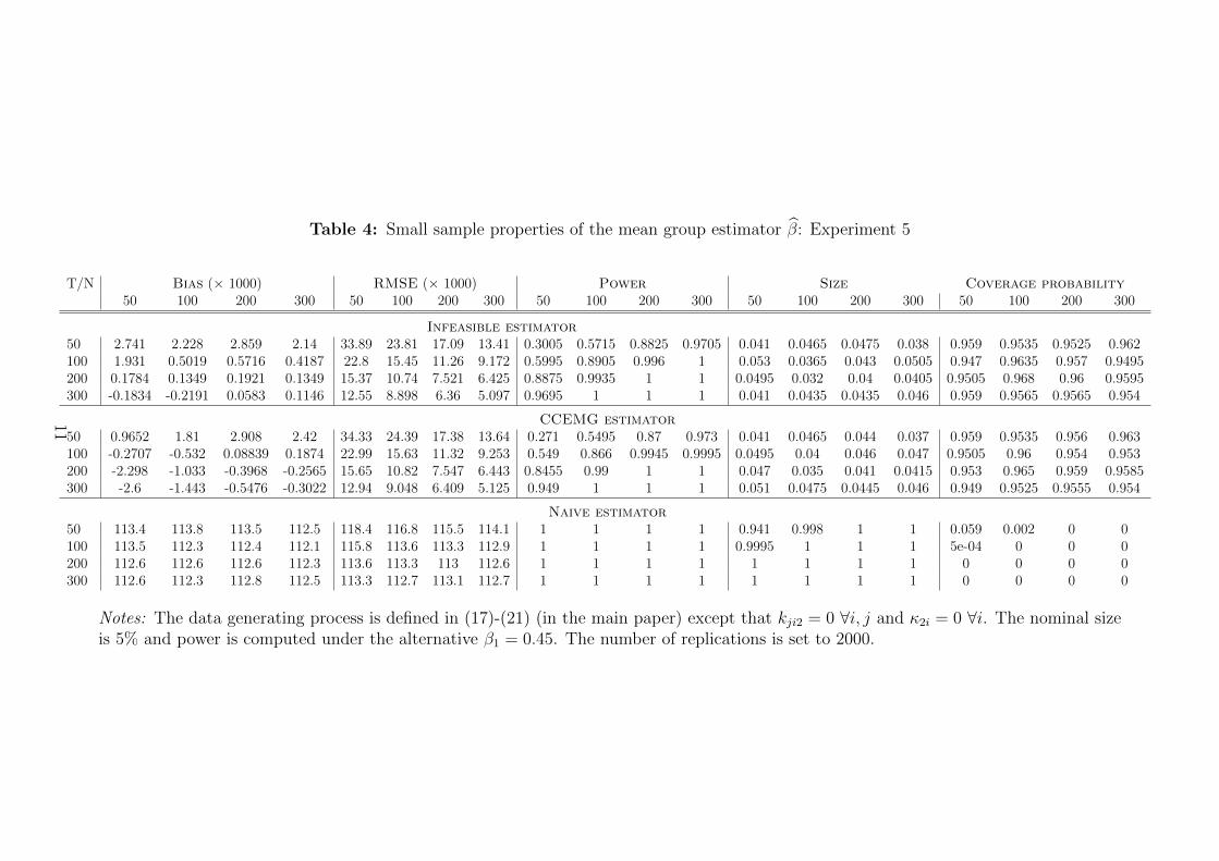
Table 4: Small sample properties of the mean group estimator β: Experiment 5

T/N Bias (× 1000) RMSE (× 1000) Power Size Coverage probability50 100 200 300 50 100 200 300 50 100 200 300 50 100 200 300 50 100 200 300

Infeasible estimator50 2.741 2.228 2.859 2.14 33.89 23.81 17.09 13.41 0.3005 0.5715 0.8825 0.9705 0.041 0.0465 0.0475 0.038 0.959 0.9535 0.9525 0.962100 1.931 0.5019 0.5716 0.4187 22.8 15.45 11.26 9.172 0.5995 0.8905 0.996 1 0.053 0.0365 0.043 0.0505 0.947 0.9635 0.957 0.9495200 0.1784 0.1349 0.1921 0.1349 15.37 10.74 7.521 6.425 0.8875 0.9935 1 1 0.0495 0.032 0.04 0.0405 0.9505 0.968 0.96 0.9595300 -0.1834 -0.2191 0.0583 0.1146 12.55 8.898 6.36 5.097 0.9695 1 1 1 0.041 0.0435 0.0435 0.046 0.959 0.9565 0.9565 0.954

CCEMG estimator50 0.9652 1.81 2.908 2.42 34.33 24.39 17.38 13.64 0.271 0.5495 0.87 0.973 0.041 0.0465 0.044 0.037 0.959 0.9535 0.956 0.963100 -0.2707 -0.532 0.08839 0.1874 22.99 15.63 11.32 9.253 0.549 0.866 0.9945 0.9995 0.0495 0.04 0.046 0.047 0.9505 0.96 0.954 0.953200 -2.298 -1.033 -0.3968 -0.2565 15.65 10.82 7.547 6.443 0.8455 0.99 1 1 0.047 0.035 0.041 0.0415 0.953 0.965 0.959 0.9585300 -2.6 -1.443 -0.5476 -0.3022 12.94 9.048 6.409 5.125 0.949 1 1 1 0.051 0.0475 0.0445 0.046 0.949 0.9525 0.9555 0.954

Naive estimator50 113.4 113.8 113.5 112.5 118.4 116.8 115.5 114.1 1 1 1 1 0.941 0.998 1 1 0.059 0.002 0 0100 113.5 112.3 112.4 112.1 115.8 113.6 113.3 112.9 1 1 1 1 0.9995 1 1 1 5e-04 0 0 0200 112.6 112.6 112.6 112.3 113.6 113.3 113 112.6 1 1 1 1 1 1 1 1 0 0 0 0300 112.6 112.3 112.8 112.5 113.3 112.7 113.1 112.7 1 1 1 1 1 1 1 1 0 0 0 0

Notes: The data generating process is defined in (17)-(21) (in the main paper) except that kji2 = 0 ∀i, j and κ2i = 0 ∀i. The nominal sizeis 5% and power is computed under the alternative β1 = 0.45. The number of replications is set to 2000.

11

Table 5: Small sample properties of the marginal effect ME: Experiment 4

T/N Bias (× 1000) RMSE (× 1000)50 100 200 300 50 100 200 300

Infeasible estimator50 -4.939 -4.988 -4.945 -4.932 10.07 7.935 6.572 6.071100 -2.63 -2.426 -2.451 -2.412 6.627 4.859 3.864 3.451200 -1.231 -1.146 -1.193 -1.216 4.334 3.157 2.4 2.087300 -0.8167 -0.9001 -0.8656 -0.9018 3.458 2.563 1.922 1.651

CCEMG estimator50 -5.156 -5.015 -4.912 -4.96 10.06 7.908 6.482 6.087100 -2.663 -2.493 -2.457 -2.43 6.666 4.881 3.875 3.449200 -1.264 -1.176 -1.204 -1.222 4.411 3.19 2.416 2.108300 -0.9125 -0.9155 -0.903 -0.9022 3.542 2.617 1.949 1.672

Naive estimator50 54.03 54.25 54.07 53.73 55.17 55.17 54.87 54.46100 57.75 57.95 58.01 58.21 58.32 58.37 58.38 58.55200 59.99 59.9 59.97 59.97 60.27 60.1 60.15 60.14300 60.52 60.38 60.53 60.49 60.7 60.52 60.64 60.61

Linear probability estimator50 4.402 4.511 4.652 4.57 10.16 7.901 6.498 5.96100 2.369 2.574 2.565 2.575 6.82 5.066 4.039 3.636200 1.296 1.401 1.365 1.368 4.527 3.356 2.553 2.232300 0.812 0.8319 0.8303 0.8355 3.631 2.657 1.95 1.664

Notes: The mean group estimator of the average marginal effect is is reported. The data generatingprocess is defined in (17)-(21) and (22) (in the main paper). The number of replications is set to2000.

12

Table 6: Small sample properties of the marginal effect ME: Experiment 5

T/N Bias (× 1000) RMSE (× 1000)50 100 200 300 50 100 200 300

Infeasible estimator50 -4.699 -4.763 -4.657 -4.821 10.04 7.882 6.44 5.971100 -2.127 -2.531 -2.511 -2.549 6.709 5.037 4.044 3.619200 -1.262 -1.289 -1.274 -1.286 4.599 3.35 2.509 2.242300 -0.9358 -0.9462 -0.8643 -0.8519 3.759 2.741 2.037 1.703

CCEMG estimator50 -5.962 -5.954 -5.863 -6.014 10.76 8.716 7.395 6.977100 -2.843 -3.216 -3.225 -3.244 7.028 5.451 4.532 4.148200 -1.672 -1.66 -1.652 -1.662 4.76 3.517 2.723 2.477300 -1.195 -1.2 -1.119 -1.11 3.872 2.847 2.162 1.849

Naive estimator50 40.28 40.56 40.45 40.03 41.5 41.38 41.04 40.56100 44.19 43.91 43.92 43.82 44.74 44.25 44.19 44.05200 45.81 45.84 45.82 45.75 46.06 46.01 45.94 45.85300 46.49 46.36 46.53 46.41 46.65 46.47 46.61 46.48

Linear probability estimator50 4.937 4.867 4.945 4.805 10.63 8.276 6.815 6.093100 2.921 2.508 2.51 2.492 7.253 5.199 4.134 3.663200 1.263 1.279 1.294 1.28 4.745 3.441 2.586 2.275300 0.7918 0.791 0.857 0.87 3.859 2.752 2.082 1.734

Notes: The mean group estimator of the average marginal effect is is reported. The data generatingprocess is defined in (17)-(21) (in the main paper) except that kji2 = 0 ∀i, j and κ2i = 0 ∀i. Thenumber of replications is set to 2000.

13

Table 7: Small sample properties of the marginal effect ME: Experiment 2

T/N Bias (× 1000) RMSE (× 1000)50 100 200 300 50 100 200 300

Infeasible estimator50 -4.741 -4.475 -4.7 -4.618 10.2 7.754 6.463 5.827100 -2.622 -2.282 -2.425 -2.409 6.707 4.909 3.868 3.424200 -1.268 -1.253 -1.313 -1.304 4.476 3.286 2.546 2.194300 -0.9855 -0.8788 -0.7807 -0.8276 3.626 2.627 1.937 1.633

CCEMG estimator50 -4.727 -4.542 -4.78 -4.672 10.25 7.779 6.516 5.86100 -2.629 -2.333 -2.454 -2.432 6.764 4.935 3.903 3.445200 -1.336 -1.308 -1.35 -1.338 4.575 3.336 2.589 2.219300 -1.064 -0.9193 -0.8168 -0.851 3.673 2.665 1.964 1.648

Naive estimator50 58.65 58.76 58.74 58.45 59.42 59.3 59.14 58.82100 62.27 62.64 62.62 62.55 62.65 62.91 62.81 62.73200 64.44 64.45 64.38 64.34 64.62 64.57 64.47 64.43300 64.96 65.03 65.12 65.12 65.07 65.11 65.18 65.17

Linear probability estimator50 5.321 5.5 5.257 5.382 11.03 8.676 7.041 6.571100 2.726 2.936 2.806 2.847 7.057 5.369 4.222 3.827200 1.328 1.407 1.34 1.355 4.684 3.468 2.626 2.264300 0.7718 0.9124 0.992 0.9621 3.68 2.719 2.082 1.742

Notes: The mean group estimator of the average marginal effect is reported. The data generatingprocess is defined in (17)-(21) (in the main paper) except that β1i = 0.5, for all i. The number ofreplications is set to 2000.

14

Table 8: Small sample properties of the marginal effect ME: Experiment 3

T/N Bias (× 1000) RMSE (× 1000)50 100 200 300 50 100 200 300

Infeasible estimator50 -4.954 -4.816 -4.75 -4.867 10.01 7.908 6.449 6.085100 -2.297 -2.499 -2.527 -2.469 6.54 5.096 4.029 3.582200 -1.088 -1.267 -1.356 -1.176 4.451 3.223 2.554 2.094300 -0.7677 -0.8723 -0.8377 -0.8485 3.592 2.663 1.949 1.685

CCEMG estimator50 -6.268 -6.303 -6.2 -6.24 10.68 8.915 7.572 7.232100 -3.381 -3.574 -3.594 -3.515 7.047 5.732 4.77 4.367200 -1.975 -2.096 -2.229 -2.034 4.813 3.652 3.115 2.682300 -1.55 -1.643 -1.594 -1.618 3.955 3.071 2.393 2.204

Naive estimator50 36.45 36.53 36.5 36.91 38.17 37.86 37.56 37.9100 40.32 39.82 40.22 39.99 41.16 40.46 40.69 40.48200 42.07 41.96 41.72 42 42.47 42.25 41.96 42.22300 42.32 42.34 42.47 42.46 42.59 42.54 42.63 42.61

Linear probability estimator50 4.269 4.249 4.381 4.296 10.02 7.887 6.366 5.808100 2.259 2.009 1.987 2.088 6.83 5.049 3.796 3.399200 0.9125 0.7905 0.649 0.8506 4.57 3.164 2.33 1.986300 0.4143 0.2925 0.3499 0.3362 3.726 2.657 1.858 1.56

Notes: The mean group estimator of the average marginal effect is reported. The data generatingprocess is defined in (17)-(21) (in the main paper) except that kji2 ∼ NID(0, 0.1). The number ofreplications is set to 2000.

15

Table 9: The effect of yields on bond issuance for US firms: controlling for liquidity

Pre-crisis Post-crisisAll Financial Other All Financial Other

Coefficient estimatesYield -0.127 -0.062 -0.184 -0.05 -0.06 -0.09

(-1.727) (-0.394) (-2.116) (-1.327) (-1.046) (-1.887)Size -0.073 -0.049 -0.09 -0.077 -0.051 -0.068

(-0.403) (-1.475) (-0.35) (-0.512) (-1.206) (-0.324)Liquidity 2.474 2.398 2.604 15.561 -3.419 21.484

(4.57) (2.257) (3.712) (1.062) (-0.724) (1.072)Marginal effects

Yield -0.016 -0.001 -0.022 -0.009 -0.004 -0.015Size -0.004 -0.01 -0.002 -0.011 -0.009 -0.01Liquidity 0.39 0.456 0.389 4.79 -0.82 6.627

Observations 321 62 225 375 72 270

Notes: The dependent variable is 1 if a firm issues a bond in a particular month and zero otherwise.Yield is the firm-specific corporate bond yield, size is measured by assets/1000 and liquidity is theshare of current debt among total debt. All specifications include a measure of credit supply (leveragein the broker-dealer market), the federal funds rate (pre-crisis only) and the change in Federal ReserveHoldings of Treasury Notes (post-crisis only) as common factors. Columns (1) and (4) use all firms,(2) and (5) use financial sector firms and (3) and (6) use all other firms (excluding mining andagriculture). t-statistics are shown in parenthesis.

16

Table 10: The effect of yields on bond issuance for US firms: corporate spreads instead of yields

Pre-crisis Post-crisisAll Financial Other All Financial Other

Coefficient estimatesSpread -0.115 -0.261 -0.137 -0.044 -0.013 -0.098

(-1.452) (-1.334) (-1.56) (-1.049) (-0.224) (-1.845)Size 0.085 -0.011 0.13 -0.23 -0.027 -0.29

(0.337) (-0.38) (0.363) (-3.18) (-0.473) (-2.965)Marginal effects

Spread -0.016 -0.029 -0.018 -0.008 0.002 -0.016Size 0.02 -0.004 0.032 -0.027 -0.006 -0.034

Observations 321 62 225 378 72 273

Notes: The dependent variable is 1 if a firm issues a bond in a particular month and zero otherwise.Spread is the firm-specific corporate bond yield minus the federal funds rate and size is measuredby assets/1000. All specifications include a measure of credit supply (leverage in the broker-dealermarket) and the change in Federal Reserve Holdings of Treasury Notes (post-crisis only) as commonfactors. Columns (1) and (4) use all firms, (2) and (5) use financial sector firms and (3) and (6) useall other firms (excluding mining and agriculture). t-statistics are shown in parenthesis.

17

Table 11: The effect of yields on bond issuance for US firms: alternative sample choices

a) Firms with at least 20 time series observationsPre-crisis Post-crisis

All Financial Other All Financial Other

Coefficient estimatesYield -0.166 -0.118 -0.216 -0.057 -0.025 -0.109

(-1.972) (-0.691) (-2.114) (-1.382) (-0.405) (-2.099)Size 0.043 0.063 0.031 -0.22 -0.009 -0.278

(0.199) (0.935) (0.103) (-2.921) (-0.117) (-2.755)Marginal effects

Yield -0.02 -0.001 -0.026 -0.01 -0.002 -0.017Size -0.028 -0.004 -0.035 -0.028 -0.004 -0.035

Observations 337 64 237 387 74 279

b) Firms with at least 40 time series observationsPre-crisis Post-crisis

All Financial Other All Financial Other

Coefficient estimatesYield -0.163 -0.193 -0.216 -0.034 -0.022 -0.083

(-1.995) (-1.149) (-2.245) (-0.869) (-0.349) (-1.695)Size 0.105 0.022 0.12 -0.174 -0.014 -0.222

(0.454) (0.722) (0.368) (-2.369) (-0.274) (-2.219)Marginal effects

Yield -0.02 -0.016 -0.026 -0.006 0.001 -0.013Size 0.023 0 0.031 -0.02 -0.002 -0.026

Observations 301 58 212 366 70 263

Notes: The dependent variable is 1 if a firm issues a bond in a particular month and zero otherwise.Yield is the firm-specific corporate bond yield and size is measured by assets/1000. All specificationsinclude a measure of credit supply (leverage in the broker-dealer market), the federal funds rate(pre-crisis only) and the change in Federal Reserve Holdings of Treasury Notes (post-crisis only) ascommon factors. Columns (1) and (4) use all firms, (2) and (5) use financial sector firms and (3)and (6) use all other firms (excluding mining and agriculture). t-statistics are shown in parenthesis.

18

Table 12: The effect of yields on bond issuance for US firms: firms with at least 2 issuances

Pre-crisis Post-crisisAll Financial Other All Financial Other

Coefficient estimatesYield -0.137 -0.252 -0.139 -0.066 0.034 -0.152

(-1.195) (-1.175) (-0.981) (-1.291) (0.391) (-2.424)Size 0.108 -0.025 0.137 -0.181 -0.096 -0.216

(0.392) (-0.695) (0.353) (-2.312) (-2.351) (-1.999)Marginal effects

Yield -0.02 -0.019 -0.021 -0.011 0.009 -0.024Size 0.021 -0.007 0.03 -0.023 -0.015 -0.027

Observations 240 48 170 250 50 180

Notes: The dependent variable is 1 if a firm issues a bond in a particular month and zero otherwise.Yield is the firm-specific corporate bond yield and size is measured by assets/1000. All specificationsinclude a measure of credit supply (leverage in the broker-dealer market), the federal funds rate(pre-crisis only) and the change in Federal Reserve Holdings of Treasury Notes (post-crisis only) ascommon factors. Columns (1) and (4) use all firms, (2) and (5) use financial sector firms and (3)and (6) use all other firms (excluding mining and agriculture). t-statistics are shown in parenthesis.

19