Discussion PaperDeutsche BundesbankNo 02/2013

A distribution-free test for outliers

Bertrand Candelon(Maastricht University)

Norbert Metiu(Deutsche Bundesbank)

Discussion Papers represent the authors‘ personal opinions and do notnecessarily reflect the views of the Deutsche Bundesbank or its staff.

Editorial Board: Klaus Düllmann

Heinz Herrmann

Christoph Memmel

Deutsche Bundesbank, Wilhelm-Epstein-Straße 14, 60431 Frankfurt am Main,

Postfach 10 06 02, 60006 Frankfurt am Main

Tel +49 69 9566-0

Please address all orders in writing to: Deutsche Bundesbank,

Press and Public Relations Division, at the above address or via fax +49 69 9566-3077

Internet http://www.bundesbank.de

Reproduction permitted only if source is stated.

ISBN 978–3–86558–881–4 (Printversion)

ISBN 978–3–86558–882–1 (Internetversion)

Non-technical summary

Statistical data analysis usually begins with the collection of observations from a cer-tain population. However, the sampling process is subject to numerous sources of error.Therefore, the data collected may contain some unusually small or large observations,so-called outliers. Determining whether a data set contains one or more outliers is achallenge commonly faced in applied statistics. This is a particularly difficult task if theproperties of the underlying population are not known. Nevertheless, in many empiricalanalyzes, the assumption that the data come from a particular population is too restrictiveor unrealistic.

This paper develops a statistical test for outliers in data drawn from an unknownpopulation. Our methodology relies on a nonparametric bootstrap procedure. Simu-lation experiments show that the proposed test detects outliers correctly whatever theunderlying population, even for relatively small samples. Consequently, our test could beinstrumental in a wide range of empirical applications where few observations are availableand the underlying population is unknown.

The empirical performance of the test is illustrated by means of two examples in thefields of aeronautics and macroeconomics. Specifically, our second example investigatesannual inflation rates for Germany from 1428 to 2010. The nearly six centuries of mon-etary history under study witnessed several episodes of hyperinflation, which constitutepotential outliers in the sense, that these observations do not belong to the same pop-ulation as the others. Indeed, we find six outliers in the sample. The earliest outlieroccurred in 1621, at the peak year of the Kipper- und Wipperzeit (Tipper and SeesawTime), a monetary crisis in the Holy Roman Empire between 1619 and 1623, which wascharacterized by hyperinflation through debasement of commodity (gold, silver, and cop-per) money. Furthermore, we find that the infamous hyperinflation in the early 20thcentury, and its collapse, was characterized by outlying annual inflation rates in 1917,1920, 1922, 1923, and 1924, whereas other historical periods with high inflation/deflationare not identified as outliers.

Nicht-technische Zusammenfassung

Die Analyse statistischer Daten beginnt in der Regel mit der Erhebung von Beobachtungenaus einer bestimmten Grundgesamtheit. Der Prozess der Stichprobenerhebung unterliegtjedoch einer Reihe von Fehlerquellen. Aus diesem Grund konnen die erfassten Dateneinige ungewohnlich niedrige oder hohe Werte enthalten, die sogenannten Ausreißer. DieFrage, ob ein Datensatz einen oder mehrere Ausreißer enthalt, ist in der angewandtenStatistik ein weitverbreitetes Problem. Sie erweist sich als besonders schwierig, wenn dieMerkmale der zugrunde liegenden Grundgesamtheit nicht bekannt sind. Gleichwohl ist invielen empirischen Untersuchungen die Annahme, dass die Daten aus einer bestimmtenGrundgesamtheit stammen, zu restriktiv bzw. unrealistisch.

In der vorliegenden Arbeit wird ein statistischer Test entwickelt, um Daten aus ei-ner unbekannten Grundgesamtheit auf Ausreißer hin zu untersuchen. Dabei kommt einnichtparametrisches Bootstrap-Verfahren zur Anwendung. Simulationsexperimente zei-gen, dass der vorgeschlagene Test Ausreißer korrekt anzeigt, und zwar ungeachtet derzugrunde liegenden statistischen Masse und sogar fur vergleichsweise kleine Stichproben.Der Test konnte also fur eine Vielzahl empirischer Anwendungen, bei denen nur wenigeBeobachtungen verfugbar sind und die Grundgesamtheit nicht bekannt ist, hilfreich sein.

Die empirische Leistungsfahigkeit des Tests wird an zwei Beispielen aus den BereichenLuftfahrt und Makrookonomie verdeutlicht. Konkret werden dazu im zweiten Beispiel diejahrlichen Inflationsraten in Deutschland im Zeitraum von 1428 bis 2010 untersucht. Diehier betrachteten rund sechs Jahrhunderte Wahrungsgeschichte umfassen mehrere Phasender Hyperinflation, die insofern potenzielle Ausreißer darstellen, als sie nicht zur selbenGrundgesamtheit gehoren wie die anderen beobachteten Werte. Tatsachlich finden sich inder Stichprobe sechs Ausreißer. Der erste Ausreißer lasst sich fur das Jahr 1621 feststellen,auf dem Hohepunkt der Kipper- und Wipperzeit, einer Krise des Munzwesens im HeiligenRomischen Reich in der Zeit von 1619 bis 1623, in der es zu einer Hyperinflation durch eineEntwertung des Warengeldes (Gold, Silber und Kupfer) kam. Als weiteres Ergebnis lasstsich festhalten, dass die beruchtigte Hyperinflation und der Zusammenbruch Anfang des20. Jahrhunderts durch Ausreißer bei den jahrlichen Preissteigerungsraten in den Jahren1917, 1920, 1922, 1923 und 1924 gekennzeichnet war, wahrend andere historische Episo-den mit hoher Inflation/Deflation nicht als Ausreißer identifiziert werden.

Bundesbank Discussion Paper No /2013

A Distribution-Free Test for Outliers∗

Bertrand CandelonMaastricht University

Norbert MetiuDeutsche Bundesbank

Abstract

Determining whether a data set contains one or more outliers is a challenge com-monly faced in applied statistics. This paper introduces a distribution-free test formultiple outliers in data drawn from an unknown data generating process. Besides,a sequential algorithm is proposed in order to identify the outlying observations inthe sample. Our methodology relies on a two-stage nonparametric bootstrap pro-cedure. Monte Carlo experiments show that the proposed test has good asymptoticproperties, even for relatively small samples and heavy tailed distributions. Thenew outlier detection test could be instrumental in a wide range of statistical ap-plications. The empirical performance of the test is illustrated by means of twoexamples in the fields of aeronautics and macroeconomics.

Keywords: Bootstrap, mode testing, nonparametric statistics, outlier detection.

JEL classification: C14.

∗Contact address: Department of Economics, Maastricht University, PO Box 616, 6200MD, Maastricht, The Netherlands. Research Centre, Deutsche Bundesbank, Wilhelm-Epstein-Straße 14, 60431 Frankfurt am Main, Germany. E-Mail: b.candelon@maastrichtuniversity.nl, nor-bert.metiu@bundesbank.de. The authors thank Don Harding, Jan Piplack, participants of the 2009Econometric Society Australasian Meeting in Canberra, the 26th Symposium on Money, Banking andFinance in Orleans, the Third Methods in International Finance Network Annual Workshop in Luxem-bourg, and seminars at the University of Rome ”Tor Vergata” and Maastricht University for commentsand suggestions. Discussion Papers represent the authors’ personal opinions and do not necessarily reflectthe views of the Deutsche Bundesbank or its staff.

02

1 Introduction

Determining whether a data set contains one or more outliers is a challenge commonlyfaced in applied statistics. This is a particularly difficult task if the underlying data gen-erating process (DGP) is unknown, since the corresponding probability density function(pdf) can have a variety of shapes in its tails. Nevertheless, the assumption of a particularDGP is often too restrictive or unrealistic. To tackle this issue, a distribution-free test foroutliers in large samples has been proposed by Walsh (1959). However, the problem ofnonparametric rejection of outliers is exacerbated in finite samples, i.e., when the numberof observations is relatively small.1 This highlights the need for a distribution-free testfor outliers in small samples, and our objective is to fill this gap.

Building on earlier work by Singh and Xie (2003) and Silverman (1981), we proposea novel nonparametric test for multiple outliers in data drawn from an unknown DGP.Besides, a sequential algorithm is proposed in order to identify the outlying observations inthe sample. The new outlier test relies on a two-stage nonparametric bootstrap procedure.Monte Carlo experiments show that the test has good asymptotic properties, even forrelatively small samples and heavy tailed distributions. Our simulations also reveal theimportance of a scaling parameter for finite sample performance. We believe that theproposed test could be instrumental in a wide range of statistical applications where fewobservations are available and the underlying DGP is unknown.

The remaining sections are organized as follows. Section 2 introduces the elemen-tary statistical definitions and describes the new outlier test. In Section 3, we explorethe asymptotic properties of the test in a Monte Carlo experiment. Section 4 presentstwo empirical examples using aeronautic and macroeconomic data. Finally, concludingremarks are contained in Section 5.

2 The Bootlier test

Consider a sample of observations labeled Y = [Y1, ..., Yn], where n = 1, 2, ..., N . Thecumulative distribution function (cdf) that generates this sequence, FY (.), is unknown. Ifany observation Yi is not distributed according to FY (.), it is considered as an outlier. Wedevelop a two-step method to test for outliers in Y, where the sample is potentially smalland the underlying distribution FY (.) is not known. First, we construct a test for thepresence of one or more outliers, building on two established statistical methods (Singhand Xie, 2003; Silverman, 1981). Second, we use a sequential algorithm to determine thenumber of outlying observations and to locate them in Y.

2.1 A bootstrap based outlier detection plot

A characterizing property of bootstrap resampling is that, when there is an outlier ina data set, it is contained in only a subset of bootstrap resamples. The outlier causesa significant increase in the sample mean of the bootstrap resample, which makes thebootstrap histogram of the sample mean a mixture distribution with more than onemode. Exploiting this feature, Singh and Xie (2003) propose a graphical tool denoted

1See Barnett and Lewis (1994) for an overview of outlier detection and finite sample.

1

Bootstrap Based Outlier Detection Plot (or simply ’Bootlier plot’), which can suggest thepresence of at least one (but possibly more) outlier(s) in a sample drawn from an unknowndistribution. However, unless the outlier(s) is (are) very severe, the multimodality ofthe bootstrap histogram is not quite visible. Therefore, Singh and Xie (2003) proposebootstrapping a statistic termed ’mean - trimmed mean’ (MTM), and inspecting themodality of the MTM’s density for outliers.

The Bootlier plot is obtained as follows. Let Yb = [Y b1 , ..., Y

bn ] (b = 1, 2, ..., B) denote

the bootstrap counterpart of Y. First, consider the k-trimmed mean of the bth bootstrapresample Yb, which is computed by taking the mean after removing the k smallest andlargest observations from Yb:

Yb(k) =

1

n− 2k

n−k∑i=k+1

Y b(i), (1)

where Y b(i) are the (ascending) order statistics and k is some trimming value.2 The MTM

of the bth bootstrap resample, M b, is the difference between the arithmetic mean and thek-trimmed mean:

M b =1

n

n∑i=1

Y bi − Y

b(k). (2)

By construction, the pdf of M b, fM(.), is very sensitive to unusually small or large obser-vations – outliers – in the sample Y. In particular, Singh and Xie (2003) show that, inthe presence of outlier(s), the limiting bootstrap distribution of M b can be expressed as amixture of normal distributions. Therefore, if there is a minimum amount of separationbetween the outliers and the remainder of the sample, then the mixture density – theBootlier plot – will be characterized by several modes.3 Hence, fM(.) typically exhibitsone mode associated with FY (.) and at least another mode corresponding to the outlier(s).Consequently, testing for the presence of outlier(s) in Y is equivalent to testing for themodality of the probability density function fM(.). If fM(.) is unimodal, the sample Y isfree of outliers, while if fM(.) is multimodal, the presence of outliers in Y is confirmed.However, note that the number of modes does not necessarily match the number of out-liers. Typically, several outliers of the same magnitude will be located around the samepole and only one mode will appear in the probability density function fM(.). It is thusnot correct to associate a given number of outliers with the same number of modes in thedensity fM(.).

Nevertheless, determining the modality of the bootstrap density absent an assumptionfor the functional form of FY (.) is not straightforward. Singh and Xie (2003) introducea ’Bootlier index’ as a rule-of-thumb tool in order to determine the degree of bumpi-ness of the density function, but they do not provide a statistical framework to test formultimodality and thus for the presence of outliers. They state that ”Formal tests foroutliers can be constructed with the Bootlier index as test statistic under a distribu-tional assumption” (page 543). Our approach is different. In what follows we consider adistribution-free test for the null of no outliers.

2Following Singh and Xie (2003), we set k = 2 in our applications.3We explore the degree of separation in a Monte Carlo experiment by introducing outliers of different

magnitudes into samples drawn from a known distribution.

2

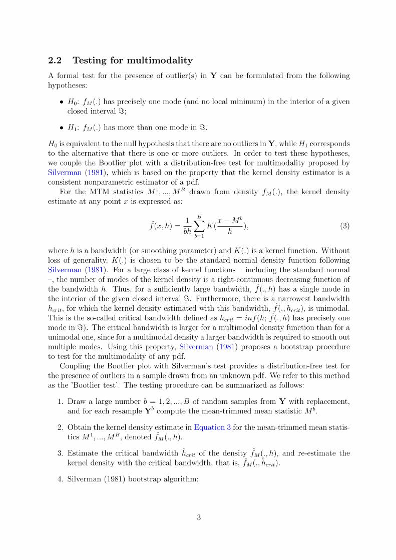
2.2 Testing for multimodality

A formal test for the presence of outlier(s) in Y can be formulated from the followinghypotheses:

• H0: fM(.) has precisely one mode (and no local minimum) in the interior of a givenclosed interval =;

• H1: fM(.) has more than one mode in =.

H0 is equivalent to the null hypothesis that there are no outliers in Y, whileH1 correspondsto the alternative that there is one or more outliers. In order to test these hypotheses,we couple the Bootlier plot with a distribution-free test for multimodality proposed bySilverman (1981), which is based on the property that the kernel density estimator is aconsistent nonparametric estimator of a pdf.

For the MTM statistics M1, ...,MB drawn from density fM(.), the kernel densityestimate at any point x is expressed as:

f(x, h) =1

bh

B∑b=1

K(x−M b

h), (3)

where h is a bandwidth (or smoothing parameter) and K(.) is a kernel function. Withoutloss of generality, K(.) is chosen to be the standard normal density function followingSilverman (1981). For a large class of kernel functions – including the standard normal–, the number of modes of the kernel density is a right-continuous decreasing function ofthe bandwidth h. Thus, for a sufficiently large bandwidth, f(., h) has a single mode inthe interior of the given closed interval =. Furthermore, there is a narrowest bandwidthhcrit, for which the kernel density estimated with this bandwidth, f(., hcrit), is unimodal.This is the so-called critical bandwidth defined as hcrit = inf(h; f(., h) has precisely onemode in =). The critical bandwidth is larger for a multimodal density function than for aunimodal one, since for a multimodal density a larger bandwidth is required to smooth outmultiple modes. Using this property, Silverman (1981) proposes a bootstrap procedureto test for the multimodality of any pdf.

Coupling the Bootlier plot with Silverman’s test provides a distribution-free test forthe presence of outliers in a sample drawn from an unknown pdf. We refer to this methodas the ’Bootlier test’. The testing procedure can be summarized as follows:

1. Draw a large number b = 1, 2, ..., B of random samples from Y with replacement,and for each resample Yb compute the mean-trimmed mean statistic M b.

2. Obtain the kernel density estimate in Equation 3 for the mean-trimmed mean statis-tics M1, ...,MB, denoted fM(., h).

3. Estimate the critical bandwidth hcrit of the density fM(., h), and re-estimate thekernel density with the critical bandwidth, that is, fM(., hcrit).

4. Silverman (1981) bootstrap algorithm:

3

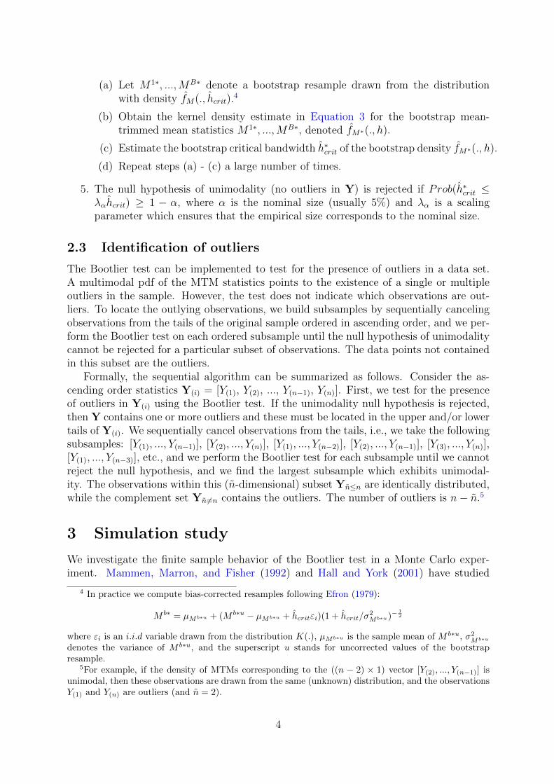
(a) Let M1∗, ...,MB∗ denote a bootstrap resample drawn from the distributionwith density fM(., hcrit).

4

(b) Obtain the kernel density estimate in Equation 3 for the bootstrap mean-trimmed mean statistics M1∗, ...,MB∗, denoted fM∗(., h).

(c) Estimate the bootstrap critical bandwidth h∗crit of the bootstrap density fM∗(., h).

(d) Repeat steps (a) - (c) a large number of times.

5. The null hypothesis of unimodality (no outliers in Y) is rejected if Prob(h∗crit ≤λαhcrit) ≥ 1 − α, where α is the nominal size (usually 5%) and λα is a scalingparameter which ensures that the empirical size corresponds to the nominal size.

2.3 Identification of outliers

The Bootlier test can be implemented to test for the presence of outliers in a data set.A multimodal pdf of the MTM statistics points to the existence of a single or multipleoutliers in the sample. However, the test does not indicate which observations are out-liers. To locate the outlying observations, we build subsamples by sequentially cancelingobservations from the tails of the original sample ordered in ascending order, and we per-form the Bootlier test on each ordered subsample until the null hypothesis of unimodalitycannot be rejected for a particular subset of observations. The data points not containedin this subset are the outliers.

Formally, the sequential algorithm can be summarized as follows. Consider the as-cending order statistics Y(i) = [Y(1), Y(2), ..., Y(n−1), Y(n)]. First, we test for the presenceof outliers in Y(i) using the Bootlier test. If the unimodality null hypothesis is rejected,then Y contains one or more outliers and these must be located in the upper and/or lowertails of Y(i). We sequentially cancel observations from the tails, i.e., we take the followingsubsamples: [Y(1), ..., Y(n−1)], [Y(2), ..., Y(n)], [Y(1), ..., Y(n−2)], [Y(2), ..., Y(n−1)], [Y(3), ..., Y(n)],[Y(1), ..., Y(n−3)], etc., and we perform the Bootlier test for each subsample until we cannotreject the null hypothesis, and we find the largest subsample which exhibits unimodal-ity. The observations within this (n-dimensional) subset Yn≤n are identically distributed,while the complement set Yn6=n contains the outliers. The number of outliers is n− n.5

3 Simulation study

We investigate the finite sample behavior of the Bootlier test in a Monte Carlo exper-iment. Mammen, Marron, and Fisher (1992) and Hall and York (2001) have studied

4 In practice we compute bias-corrected resamples following Efron (1979):

M b∗ = µMb∗u + (M b∗u − µMb∗u + hcritεi)(1 + hcrit/σ2Mb∗u)−

12

where εi is an i.i.d variable drawn from the distribution K(.), µMb∗u is the sample mean of M b∗u, σ2Mb∗u

denotes the variance of M b∗u, and the superscript u stands for uncorrected values of the bootstrapresample.

5For example, if the density of MTMs corresponding to the ((n − 2) × 1) vector [Y(2), ..., Y(n−1)] isunimodal, then these observations are drawn from the same (unknown) distribution, and the observationsY(1) and Y(n) are outliers (and n = 2).

4

the asymptotic properties of the test proposed by Silverman (1981). The test is foundto be conservative, as the true probability that it incorrectly rejects the null hypothe-sis of unimodality lies below the nominal level when the scaling parameter λα equals 1.Furthermore, Fisher and Marron (2001) show that problems arise when the underlyingdistribution is heavy tailed. Therefore, we correct for the downward bias in the empiricalsize of the multimodality test by calibrating λα such that the empirical size is close to thenominal size.

Two cdfs are considered, which have different shapes in their tails.6 Samples of sizen are generated from the standard normal distribution and from the Student-t(n − 1)distribution with n−1 degrees of freedom, which has heavy mass on the tails. 1, 000 MonteCarlo replications of the Bootlier test are performed. For each Monte Carlo replication,the fM(.) density of the MTM statistics is estimated from 10, 000 bootstrap draws fromthe sample Y, and Silverman’s test is performed with 1, 000 bootstrap replications of M b∗

drawn from the distribution with density fM(., hcrit). The asymptotic sample size is setto n = 100 for ease of computer time. To explore the small sample performance of thetest, the second sample size is set to n = 10. The simulations are performed using theStatistics Toolbox in MATLAB.

First, we simulate under the null hypothesis of no outliers, in order to assess thesize properties of the Bootlier test. Table 1 reports the rejection frequencies of the nullhypothesis of no outlier. The rejection frequencies confirm the findings of Hall and York(2001) and Fisher and Marron (2001): Silverman’s modality test is undersized when thescaling parameter equals λα = 1. Moreover, the size bias increases as the sample sizeshrinks.

We calibrate λα such that the test achieves its nominal size in both large and smallsamples. Thus, Table 1 also shows the optimal – size adjusted – λoptα , which ensures anempirical size close to the nominal size of 5%. Overall, we find that λoptα is close to thevalue obtained by Hall and York (2001).7 The scaling parameters are similar for bothdistributions when n = 10. Moreover, for large n, they converge to 1, although theconvergence is slower for the fat tailed distribution.

Table 1: Monte Carlo simulation: Size

N(0,1) distribution Student-t distributionSample Size Rejec. Freq. λα Rejec. Freq. λα

n = 10 0.00 1 0.00 10.05 λoptα =1.137 0.05 λoptα =1.134

n = 100 0.01 1 0.04 10.05 λoptα =1.021 0.05 λoptα =1.070

Note: The top panel reports the rejection frequencies of the null hypothesis of no outlier for the standardnormal distribution, the bottom panel reports the rejection frequencies for the Student-t distribution withλα = 1, and with λoptα set at a nominal size of 5%.

6Our procedure requires the existence of finite means for the computation of the MTM statistic.Therefore, random variables generated from the Cauchy distribution cannot be considered, since for thelatter finite moments do not exist (see Casella and Berger, 2002).

7In Equation (4.1), on page 524, they obtain λoptα = 1.1294 for α = 5%.

5

Next, we turn to the power of the test. Table 2 shows the rejection of the nullhypothesis when data is simulated under the presence of an outlier, such that the outlierequals µ+ iσ, where µ is the sample mean of the baseline sample (absent outliers), whileσ is the sample standard deviation. The size of the outlier depends proportionally on thevalue of i (we consider i = 3.5, 4, 4.5, and 5). The power is corrected for size distortions,since the simulations are also performed with the optimal scaling parameter λoptα .

Table 2: Monte Carlo simulation: Power (size-adjusted)

N(0,1) distribution; Outlier = µ+ iσi=3.5 i=4 i=4.5 i=5

Sample Size Lambda Rejec. Freq. Rejec. Freq. Rejec. Freq. Rejec. Freq.n=10 1 0.22 1.00 1.00 1.00

λoptα 0.96 1.00 1.00 1.00n=100 1 1.00 1.00 1.00 1.00

λoptα 1.00 1.00 1.00 1.00

Student-t distribution; Outlier = µ+ iσi=3.5 i=4 i=4.5 i=5

Sample Size Lambda Rejec. Freq. Rejec. Freq. Rejec. Freq. Rejec. Freq.n=10 1 0.19 0.98 1.00 1.00

λoptα 0.41 1.00 1.00 1.00n=100 1 1.00 1.00 1.00 1.00

λoptα 1.00 1.00 1.00 1.00Note: Rejection frequencies of the null hypothesis of no outlier when the distributions are simulatedunder the presence of an outlier, with outliers specified as values corresponding to the mean µ plus itimes the size of the sample standard deviation σ (outlier = µ + iσ). The power is corrected for sizedistortions, as simulations are performed with the optimal λoptα .

Table 2 reveals that, when the test is undersized (i.e., λα = 1) and the outlier issmall in magnitude relative to the sample mean (i = 3.5), the test has moderate power.This result holds for both distributions. However, when the test is correctly sized, itgenerally attains good power (the only exception being the Student-t distribution whenboth the sample size and the outlier is small). The frequency of correct rejection of thenull hypothesis reaches 100% (for a 5% nominal size) in all cases when the outlier is atleast four times the sample standard deviation, irrespective of the distribution considered.

4 Empirical illustration

Example 1

The empirical performance of the Bootlier test is illustrated by means of two examples.First, we revisit an aeronautics data set studied earlier by Dalal, Fowlkes, and Hoadley(1989) and Singh and Xie (2003). Shortly after liftoff on January 28, 1986, the spaceshuttle Challenger disintegrated over the Atlantic Ocean. The explosion occurred due tothe leakage of an O-ring that sealed the right solid booster rocket of the vehicle, whichallowed pressurized gas from within the rocket to reach the outside, leading to combustion.

6

It has been subsequently shown that the O-rings do not seal properly at low temperatures(see Dalal et al., 1989).

Consider the recorded temperatures at which the O-rings were sealed on all 25 shuttlelaunches of the Challenger, expressed in degrees Fahrenheit:

66 70 69 80 68 67 72 73 70 57 63 70 78 67 53 67 75 70 81 76 79 75 76 58 31.

The last observation is 31oF, the temperature on the day of the explosion. This datapoint qualifies as a good candidate for being an outlier. Figure 1 shows the Bootlierplot of the full sample, which exhibits 3 modes, and the Bootlier plot of the sampleafter removing the last observation, which is unimodal. Hence, a visual inspection of theBootlier plots suggests that 31oF is indeed an outlier. Next, the Bootlier test is performedto obtain formal statistical evidence. The test for the full sample gives a p-value lowerthan 1%, indicating a clear rejection of the null hypothesis of unimodality (no outliers),while the test on the subsample which does not contain 31oF leads to a p-value of 0.21.Consequently, the null hypothesis cannot be rejected for the latter subsample, and thetemperature at which the O-rings were sealed on the day of the accident proves to be anoutlier.

Figure 1: Bootlier plots of Challenger data

−4 −3 −2 −1 0 1 20

0.1

0.2

0.3

0.4

0.5

0.6

0.7

Bootstrap MTM statistics

Ker

nel

den

sity

(a) Full sample

−1.5 −1 −0.5 0 0.5 10

0.5

1

1.5

Bootstrap MTM statistics

Ker

nel

den

sity

(b) Subsample without 31oF

Example 2

Our second example investigates macroeconomic data. We consider annual inflation rates(annual percent changes in the aggregate price level) for Germany from 1428 to 2010. Thedata come from Reinhart and Rogoff (2011) and are available on the Internet site of theAmerican Economic Association.8

Figure 2 plots the time series. In order to obtain a good visualization of the series,the data range is censored in the figure from above at 1920, 1922, and 1923 when therate of inflation was 291.45, 2715.224, and 2.11E+11 percent per annum respectively, andfrom below at 1924 when the inflation rate was -200 percent per annum. The nearly sixcenturies of monetary history under study witnessed several episodes of hyperinflation,which constitute potential outliers. At first glance, three relatively more turbulent periods

8See: http://www.aeaweb.org/articles.php?doi=10.1257/aer.101.5.1676.

7

stand out. First, the Thirty Years’ War in the early 17th century, second, the prolongedinflationary period surrounding the industrial revolution from the late 18th to the late19th century, and third, the infamous hyperinflation of the 1920s. The figure also revealsthat the most recent decades are characterized by the historically lowest and least volatileinflation. This period is often described as the ”Great Moderation”, and it coincides withthe adaption of a proactive approach toward inflation in central banking.

Figure 2: Germany: inflation, annual percent change, 1428-2010.

1450 1550 1650 1750 1850 1950

−100

−80

−60

−40

−20

0

20

40

60

80

100Percent per annum

Year

The results of the Bootlier test for the inflation data are reported in Table 3. Wefind six outliers in the data, and once we remove these from the sample, we obtain ap-value of 0.09 for the Bootlier test. The earliest outlier occurs in 1621, at the peak yearof the Kipper- und Wipperzeit (Tipper and Seesaw Time), a monetary crisis in the HolyRoman Empire between 1619 and 1623, which was characterized by hyperinflation throughdebasement of commodity (gold, silver, and copper) money. An exhaustive historicalaccount of the crisis is offered by Kindleberger (1991).

The other five outliers concentrate around the most severe hyperinflation and subse-quent collapse in German history in the early 20th century, which has been investigated ina seminal paper by Cagan (1956). Inflation peaked at approximately 211 billion percentper annum in 1923, which is the most outlying observation. Nevertheless, all outliers arerelatively severe, given that the sample mean without the outliers is 2.352 percent andthe sample standard deviation is 14.250 percent.

Table 3: Outliers in German inflation (percent per annum)

Year Outlier1621 105.2901917 98.1821920 291.4501922 2715.2241923 2.11E+111924 -200.000

Figure 3 (a) shows the Bootlier plot for the full sample. Again, the mutimodal patternis clearly visible, indicating the presence of outliers. Figure 3 (b) shows the Bootlier plotonce all outliers are removed. This figure reveals that a mere visual inspection of theBootlier plot in insufficient and may lead to misleading conclusions regarding outliers.

8

Figure 3: Bootlier plots of inflation data

−4 −2 0 2 4 6 8 10

x 108

0

0.5

1

1.5

2x 10

−9

Bootstrap MTM statistics

Ker

nel

den

sity

(a) Full sample

−0.1 −0.05 0 0.05 0.1 0.150

2

4

6

8

10

12

14

Bootstrap MTM statistics

Ker

nel

den

sity

(b) Subsample without outliers

Even though the plot exhibits a minor kink, the modality test cannot statistically rejectthe unimodality hypothesis at the conventional 5% significance level.

5 Concluding remarks

This paper has introduced a distribution-free test for outliers in statistical data drawnfrom an unknown DGP. Building on earlier work by Singh and Xie (2003) and Silverman(1981), we construct a test for the presence of one or more outliers, and we proposea sequential algorithm to determine the number of outliers as well as their location inthe sample. Monte Carlo experiments show that this new method has good asymptoticproperties, even for relatively small samples, whatever shape the underlying pdf may havein its tails.

The empirical performance of the outlier test is illustrated by means of two empiricalexamples using aeronautic and macroeconomic data. The new test could be instrumentalin a wide range of statistical applications where few observations are available and theunderlying DGP is unknown. For instance, Candelon, Metiu, and Straetmans (2012)employ the test proposed in this paper to investigate business cycle booms and depressions.

References

Barnett, V. and T. Lewis (1994). Outliers in Statistical Data (3rd ed.). Wiley Series inProbability and Statistics. Wiley.

Cagan, P. (1956). The monetary dynamics of hyperinflation. In M. Friedman (Ed.),Studies in the quantity theory of money. University of Chicago Press, Chicago.

Candelon, B., N. Metiu, and S. Straetmans (2012). Understanding economic booms anddepressions. Mimeo Maastricht University.

Casella, G. and R. L. Berger (2002). Statistical Inference (2 ed.). Duxbury AdvancedSeries. Duxbury Press.

9

Dalal, S., E. Fowlkes, and B. Hoadley (1989). Risk analysis of the space shuttle: Pre-Challenger prediction of failure. Journal of the American Statistical Association 84,945–957.

Efron, B. (1979). Bootstrap methods: Another look at the jackknife. Annals of Statis-tics 7 (1), 1–26.

Fisher, N. I. and J. S. Marron (2001). Mode testing via the excess mass estimate.Biometrika 88 (2), 499–517.

Hall, P. and M. York (2001). On the calibration of Silverman’s test for multimodality.Statistica Sinica 11, 515–536.

Kindleberger, C. (1991). The economic crisis of 1619 to 1623. Journal of EconomicHistory 51, 149–175.

Mammen, E., J. S. Marron, and N. I. Fisher (1992). Some asymptotics for multimodalitytests based on kernel density estimates. Probability Theory and Related Fields 91,115–132.

Reinhart, C. and K. Rogoff (2011). From financial crash to debt crisis. American EconomicReview 101, 1676–1706.

Silverman, B. W. (1981). Using kernel density estimates to investigate multimodality.Journal of the Royal Statistical Society, B 43 (1), 97–99.

Singh, K. and M. Xie (2003). Bootlier Plot - Bootstrap based outlier detection plot.Sankhya: The Indian Journal of Statistics 65 (3), 532–559.

Walsh, J. (1959). Large sample nonparametric rejection of outlying observations. Annalsof the Institute of Statistical Mathematics 10, 223–232.

10