A Dynamic Duverger’s Law

Jean Guillaume Forand∗ and Vikram Maheshri†

February 19, 2014

Abstract

Electoral systems promote strategic voting and affect party systems. Duverger (1951) proposedthat plurality rule leads to bi-partyism and proportional representation leads to multi-partyism.We show that in a dynamic setting, these static effects also lead to a higher option value forexisting minor parties under plurality rule, so their incentive to exit the party system is mitigatedby their future benefits from continued participation. The predictions of our model are consistentwith multiple cross-sectional predictions on the comparative number of parties under pluralityrule and proportional representation. In particular, there could be more parties under pluralityrule than under proportional representation at any point in time. However, our model makes aunique time-series prediction: the number of parties under plurality rule should be less variablethan under proportional representation. We provide extensive empirical evidence in support ofthese results.

1 Introduction

The relationship between electoral systems and the number of parties contesting elections has be-come a classic topic of study in political science. Duverger (1951), who first formulated the questionprecisely, postulated the ‘law’ that plurality rule leads to two-party competition and the com-plementary ‘hypothesis’ that plurality rule with a runoff and proportional representation favormulti-partism (see Benoit (2006) and Riker (1982)). Empirically, party systems are not observed tobe particularly stable over time: irrespective of electoral system, there is substantial longitudinalvariation in the number of parties active in a country. However, existing research, both theoretical(e.g., Feddersen (1992), Palfrey (1989)) and empirical (e.g., Lijphart (1994), Taagepera and Shugart(1989)), has focused overwhelmingly on static, cross-sectional environments.∗Department of Economics, University of Waterloo.†Department of Economics, University of Houston. We thank Scott Legree for excellent research assistance.

1

Duverger supported his law by appealing to a dynamic process in which the number of partiesis winnowed down by the combined impact of mechanical and psychological effects: plurality rulesystematically underrepresents minor parties (mechanical), and in anticipation of this fact, strategicvoters gradually desert all but two parties (psychological). In response, Chhibber and Kollman(1998) argued that when “accounting for changes in the number of national parties over time withinindividual countries, however, explanations based solely on electoral systems [...] are strained. Thesefeatures rarely change much within countries, and certainly not as often as party systems undergochange in some countries.” As important features of political environments (voters’ preferences,salient issues, party leaderships) evolve over time, changes in the number of parties over timeshould be expected. This remark still leaves open the possibility that different electoral systemsinduce systematically different party system dynamics.

In this paper, we theoretically and empirically analyze the dynamic implications of the electoralincentives underlying Duverger’s Law. We make two primary contributions. First, we develop asimple dynamic model of partisan politics that implies that plurality rule elections generate lowervariability in the number of national parties over time (or partisan churn) than more proportionalsystems. Second, we offer empirical support for this hypothesis by analyzing the relationship be-tween partisan churn and the disproportionality of electoral systems in a panel of 54 democraciessince 1945. As predicted by the model, we find that more disproportional electoral systems arerobustly associated with less entry of new parties and less exit of old parties. Together, this con-stitutes support for a reinterpretation of Duverger’s vision of party dynamics. Notably, our modeldoes not make unambiguous static predictions of the relationship between the number of compet-ing parties and the disproportionality of electoral systems. This point has been previously madein static theoretical models (Morelli (2004)) and reconciles empirical findings presented here andelsewhere.

In our model, parties function as vehicles to promote the preferred policies of ideologicallymotivated activists. Parties are formed, maintained, and possibly disbanded by their activists.Supporting a party is costly as it requires the resources necessary to run a serious campaign: re-cruiting good candidates, mobilizing party volunteers and raising advertising funds. In view of thecritique of Chhibber and Kollman (1998), the key dynamic ingredient of the model is a stochasticpolitical environment: for any number of reasons, the support garnered among the voters by thevarious policies preferred by the activists may evolve over time. It follows that activists’ incentivesto support parties to represent them may also evolve, so activists whose policy goals are currentlyout of favor with voters may disband an existing party in the hopes of forming a new party in thefuture when voters become more receptive. Since forming a new party is costlier than maintainingan existing party, being currently represented by a party generates an option value to the activists

2

who support it.We take the perspective that party systems adapt to changing political circumstances by allow-

ing the formation of parties that champion policy positions that were not represented in previouselections. In the model, the evolution of the political environment drives the entry of new partiesand exit of existing parties. In practice, variability in party systems often involves transformationsof existing parties with a corresponding reshuffling of their leadership and base. Party exit rarelytakes the form of an outright dissolution but rather of a merger with ideologically compatible op-ponents. For example, the Liberal Democrats in the United Kingdom were formed in 1988 throughthe combination of the Liberal and Social Democratic parties, and the Christian Democratic Appealwas formed in the Netherlands in 1977 through the merger of three mainstream Christian parties.Similarly, the creation of a new party often occurs through the splintering of an existing party (e.g.,the Left parties in Germany in 2007 and in France in 2008 combined various elements from existingparties on the left of the political spectrum).

Under plurality rule, the static mechanical and psychological effects favor the exit of partieswith low current (anticipated) voter support and inhibit the entry of new parties. While there issome debate on whether these effects can be separately identified (see Benoit (2002)), the impor-tance of their combined effect has been extensively documented. At the country level, the effectivenumber of parties either contesting elections or represented in legislatures is positively associated tovarious measures of the proportionality of electoral systems such as average district magnitude (seeBlais and Carty (1991), Lijphart (1994), Neto and Cox (1997), Ordeshook and Shvetsova (1994)and Taagepera and Shugart (1989)).1 At the electoral district level, measuring the importanceof strategic voting in an electoral district of magnitude M typically involves comparing the votesobtained by the candidates with the M + 1 and M + 2-ranked number of votes, i.e., the election’srunner-up and second runner-up (see Cox (1997) and Fujiwara (2011)). As noted by Cox (1997), inan equilibrium in which a district’s voters coordinate onto at most one non-winning alternative, theratio of votes for candidates with ranks M + 2 and M + 1 should be zero. Interestingly, Cox (1997)finds evidence that the proportion of districts with electoral outcomes approaching this ‘Duverger’outcome shrinks as the district magnitude M increases, suggesting that the incentives promoting,and/or the effectiveness of, strategic voting is reduced under more proportional electoral systems.These empirical results motivate the two key assumptions that differentiate plurality rule electionsfrom proportional elections in our model. First, under plurality rule, a party with a small expectedvote share in the current election suffers a minority penalty to its realized vote share. This electoraldisadvantage of small parties under plurality combines the impacts of the static mechanical andpsychological effects. Second, given any expected vote share, a newly-formed party under plurality

1District magnitude is defined as the number of representatives elected in a district.

3

rule suffers an entry penalty to its realized vote share. The incentives for strategic voting, which arestrongest under plurality rule, reflect voters’ attempts to coordinate onto competitive candidates.Since past voting behavior is likely to facilitate coordination, we posit that barriers to entry facedby new parties are higher under plurality rule.

Our model’s novel dynamic insights come from combining (i) the variation in maintenance costsfor minor parties and entry costs for new parties across electoral systems with (ii) the party supportdecisions of forward-looking activists represented by currently unpopular parties. Under pluralityrule, the current cost to minor parties of maintaining their position is high, which incentivizesparty exit. On the other hand, the option value of their position, which reflects the higher futurecosts of forming new parties, is also high, which incentivizes party maintenance. Under proportionalrepresentation, activists can respond more flexibly to changes in their current political circumstancesby disbanding the parties they support in unfavorable political environments and forming newparties when, for example, new issues become salient. As the previous discussion suggests, ourmodel makes no prediction of the number of parties in a given country at a given point in time. Infact, under plurality rule, we derive equilibria in which, in all elections at any time, there are at leastas many active parties as under proportional representation. However, all equilibria under pluralityrule feature less longitudinal variation in the number of active parties than the unique equilibriumunder proportional representation: irrespective of the current number of parties, partisan churnunder plurality rule is lower than under proportional representation.

We provide empirical support for our model with an analysis of competitive party behaviorover time in democracies with varying levels of electoral proportionality. Our data come fromthe Constituency-Level Elections (CLE) Dataset from which we construct an unbalanced panel ofelections in 54 countries since 1945 (Brancati (accessed 2013)). Our key empirical finding is thatthe proportionality of a country’s electoral system is robustly correlated to the level of partisanchurn observed in its elections. Highly proportional electoral systems such as Israel and Belgiumfeature elections with systematically greater entry and exit of parties than highly disproportionalelectoral systems such as the United States and Mexico. We subject this finding to a number ofrobustness checks and find that the dynamic relationship persists. On the other hand, we do notfind strong evidence in favor of the static prediction of Duverger’s Law. That is, although we find apositive relationship between the proportionality of an electoral system and the number of partiesthat compete in a given election, this association is not statistically significant. Hence, while theoft-cited ‘exceptions’ to Duverger’s Law (e.g., Austria, Canada) blur the cross-sectional link betweenelectoral rules and the number of parties as predicted by a number of theoretical models includingours, their longitudinal relationship, which is the novel prediction of our dynamic model, is quitestrong.

4

In the terminology of Shugart (2005), ours is a ‘macro level’ study in that we focus on parties’entry and exit decisions in elections to the national parliament. This aggregation is necessary, andour hypothesis cannot be evaluated at the electoral district-level: a serious party either participatesin elections in a large number of districts or risks failing to be considered as a legitimate nationalparty. In fact, Fujiwara (2011) demonstrates this when he finds that the electoral system (pluralityversus plurality with a runoff) has no impact on the identities of the parties competing for themayoralty of Brazilian cities. He attributes this to the fact that serious candidates are affiliated toa major national party, and all serious national parties field candidates in most mayoral elections.It has long been noted that the results of Duverger (1951) are naturally established at the districtlevel, and that his arguments establishing the ‘linkage’ of electoral systems’ effects on the numberof parties at the district level with the number of parties on the national stage are incomplete(see Cox (1997)). While a growing number of empirical studies address this linkage problem (seeChhibber and Kollman (1998), Chhibber and Murali (2006), Cox (1997)), theoretical investigationsof Duverger’s results have mostly focused on a single electoral district. In an important exception,Morelli (2004) shows that Duverger’s predictions can be reversed in a multi-district setting if thereis enough heterogeneity across districts. Our model shows that even abstracting from the linkageproblem and considering a single district, the cross-sectional predictions of Duverger can be reversedsolely due to the dynamic incentives of parties’ supporters. The key contribution in this paper isthat we recover a unique time series prediction.

While Duverger (1951) couched his arguments in dynamic terms, intertemporal approaches tothe study of comparative political systems are rare. Cox (1997) highlights the importance of thedynamic incentives of parties and politicians for understanding the limits to Duverger’s predictions,but he does not propose a particular model. Fey (1997) studies a dynamic process involving opinionpolls to show that non-Duverger equilibria of the standard static model are unstable. We are notaware of any other theoretical paper embedding the study of the number of parties in a dynamicframework. Some recent empirical studies have focused on the dynamics of the number of parties.Chhibber and Kollman (1998) show that in the United States and India, the number of partiesdecreased in periods in which the central government assumed a larger role. This result, whichcompares countries with plurality elections, is focused on providing conditions which support thelinkage from district to the national level. Reed (2001) provides evidence that at the district levelelections became increasingly bipartisan in Italy following a change of voting rule in 1993. However,Gaines (1999) finds little evidence of a trend towards local two-partism in a longitudinal analysis ofCanadian elections (see also Diwakar (2007) for the case of India).

5

2 The Dynamics of Party Entry and Exit: Model

2.1 Setup

Elections are held over an infinite horizon. Following an election at time t = 1, 2, ..., the winningparty selects a policy xt ∈ {x−1, x0, x1}, where x−1 < x0 < x1. A party j can be of one of three typesin {−1, 0, 1} (e.g., left, middle or right). Parties are formed and maintained by policy-motivatedactivists. Specifically, there are two long-lived activists of type −1 and 1, and in each period theysimultaneously decide whether or not to support a party of their type to represent them. Wemake two simplifying assumptions that allow us to focus on the incentives of these two non-centristactivists to form, maintain and disband parties. First, we assume that parties are non-strategic: ifin power, party j implements policy xj . Second, we assume that a party of type 0 is present in allelections. This simple environment allows for rich dynamics for party entry and exit, as well as forparty structures, which in any given election can feature one, two or three parties. The electoralrule, which we detail below, is either plurality rule or proportional.

At the beginning of each period, a preference state st ∈ {s−1, s0, s1} is randomly drawn. Pref-erence states capture variability in the political environment, which generates an option value toparties that maintain their electoral presence and is absent from static models. We assume thatpreference states are identically and independently distributed across periods: let Pr(st = s0) = q

and Pr(st = s1) = Pr(st = s−1) = 1−q2 for q ∈ (0, 1).2 Preference states have a straightforward

interpretation: in state sj , the party representing activist j is favored by voters. Specifically, definep, p and p such that 1 ≥ p > p > p ≥ 0, normalized such that p + p + p = 1, and let ptj representthe policy support of xj in period t. Specifically, for the two non-centrist policies xj ∈ {x−1, x1}, wedefine

ptj =

p if st = sj ,

p if st = s−j ,p+p

2 if st = s0.

Note that this implies that when the voters have non-centrist preferences (i.e., st ∈ {s−1, s1}),the policy support of the centrist policy x0 is p. Also, note that, for any preference state st,pt−1 + pt0 + pt1 = 1.

While ptj is a measure of the popularity of policy xj in the election at time t, this policy maynot be championed by a party if the activist of type j does not support a party. Conversely, a partychampioning policy xj may have an expected popularity that exceeds ptj since it may draw support

2We could allow for persistence in electoral states, although this would add computational complexity withoutaffecting our central conclusions. Likewise, the simplifying assumption that non-centrist preference states s1 and s−1

occur with equal probability allows us to exploit symmetry, but it is not essential.

6

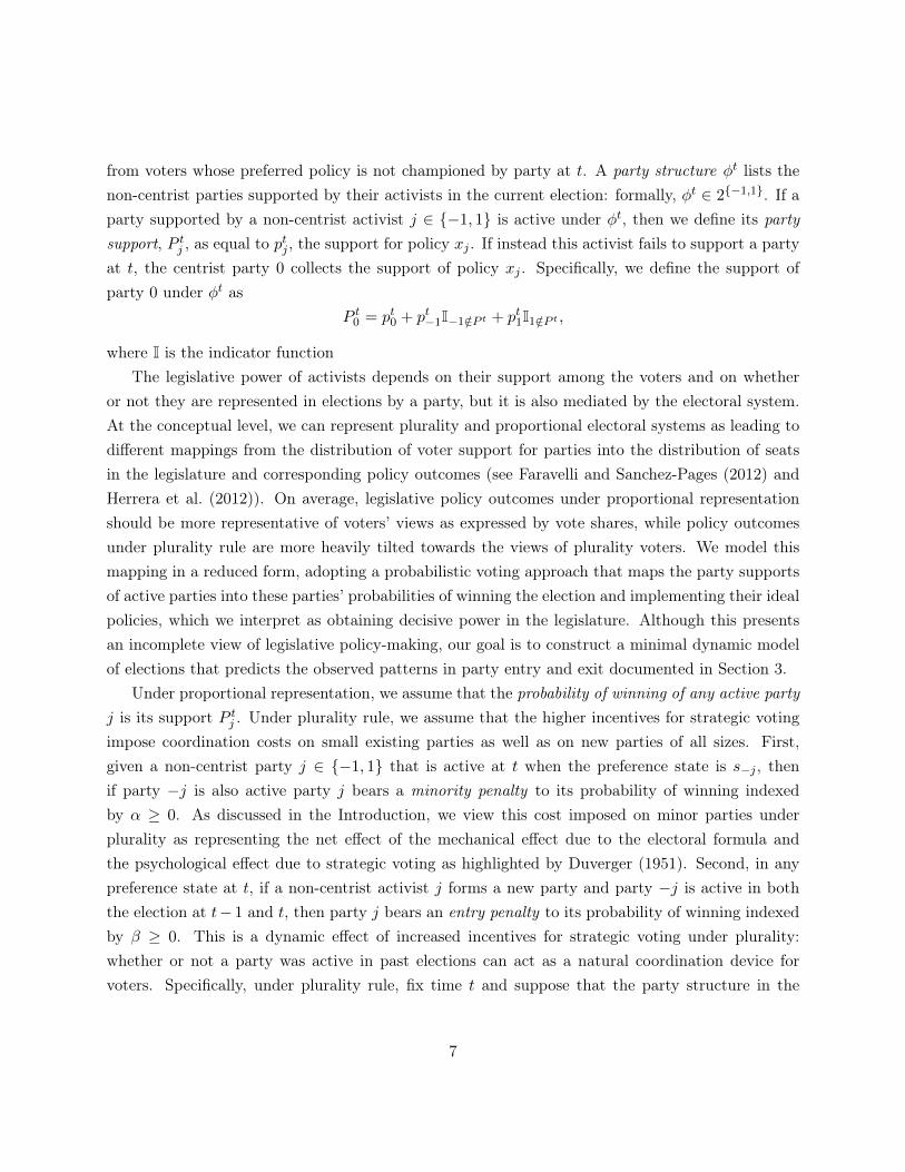
from voters whose preferred policy is not championed by party at t. A party structure φt lists thenon-centrist parties supported by their activists in the current election: formally, φt ∈ 2{−1,1}. If aparty supported by a non-centrist activist j ∈ {−1, 1} is active under φt, then we define its partysupport, P tj , as equal to p

tj , the support for policy xj . If instead this activist fails to support a party

at t, the centrist party 0 collects the support of policy xj . Specifically, we define the support ofparty 0 under φt as

P t0 = pt0 + pt−1I−1/∈P t + pt1I1/∈P t ,

where I is the indicator functionThe legislative power of activists depends on their support among the voters and on whether

or not they are represented in elections by a party, but it is also mediated by the electoral system.At the conceptual level, we can represent plurality and proportional electoral systems as leading todifferent mappings from the distribution of voter support for parties into the distribution of seatsin the legislature and corresponding policy outcomes (see Faravelli and Sanchez-Pages (2012) andHerrera et al. (2012)). On average, legislative policy outcomes under proportional representationshould be more representative of voters’ views as expressed by vote shares, while policy outcomesunder plurality rule are more heavily tilted towards the views of plurality voters. We model thismapping in a reduced form, adopting a probabilistic voting approach that maps the party supportsof active parties into these parties’ probabilities of winning the election and implementing their idealpolicies, which we interpret as obtaining decisive power in the legislature. Although this presentsan incomplete view of legislative policy-making, our goal is to construct a minimal dynamic modelof elections that predicts the observed patterns in party entry and exit documented in Section 3.

Under proportional representation, we assume that the probability of winning of any active partyj is its support P tj . Under plurality rule, we assume that the higher incentives for strategic votingimpose coordination costs on small existing parties as well as on new parties of all sizes. First,given a non-centrist party j ∈ {−1, 1} that is active at t when the preference state is s−j , thenif party −j is also active party j bears a minority penalty to its probability of winning indexedby α ≥ 0. As discussed in the Introduction, we view this cost imposed on minor parties underplurality as representing the net effect of the mechanical effect due to the electoral formula andthe psychological effect due to strategic voting as highlighted by Duverger (1951). Second, in anypreference state at t, if a non-centrist activist j forms a new party and party −j is active in boththe election at t− 1 and t, then party j bears an entry penalty to its probability of winning indexedby β ≥ 0. This is a dynamic effect of increased incentives for strategic voting under plurality:whether or not a party was active in past elections can act as a natural coordination device forvoters. Specifically, under plurality rule, fix time t and suppose that the party structure in the

7

current election is such that φt = {−1, 1}. Then the probability of winning of a non-centrist partyj is

P tj + α[Ist=sj − Ist=s−j

]+ β

[Ij∈φt−1I−j /∈φt−1 − Ij /∈φt−1I−j∈φt−1

].

Meanwhile, if φt = {j}, then the probability with which party j wins is P tj . To ensure that, forany st an active party j has a non-negative winning probability, we assume that α + β ≤ p. Notethat our formulation assumes that any coordination costs imposed on party j benefit only party−j, which implies that in any preference state, the probability of winning of party 0 under pluralityrule is P t0.

Activists are risk-neutral and have single-peaked preferences over feasible policies with a non-centrist activist of type j having ideal policy xj . Given any non-centrist activist, let u be its stagepayoff to its preferred policy, u be its stage payoff to its second-ranked policy, and u be its stagepayoff to its third-ranked policy with u > u > u. Supporting parties is costly for activists, althoughforming a new party is costlier than maintaining an existing party. This wedge between the costof maintaining an existing party and the cost of forming a new party generates an option valueto existing parties for activists. Specifically, at time t, if j ∈ φt−1, then the party maintenancecost to activist j in the electoral cycle at t is c. If instead j /∈ φt−1, then no party representedactivist j in the previous election and the party formation cost at t to activist j is c > c. Activistsdiscount future payoffs by a common factor of δ, and make party support decisions to maximizetheir expected discounted sum of payoffs, which in any election consists of the expected differencebetween its benefits from the policy implemented by the winning party and its party formation costs(where the expectation is over electoral outcomes).

2.2 Strategies and Equilibrium

We focus on Markov perfect equilibria in pure strategies in which activists condition their partyformation and maintenance decisions at time t on the payoff-relevant state (st, φt−1): the currentpreference state and the previous party structure. For a non-centrist activist j, a strategy is σj :

{s−1, s0, s1} × 2{−1,1} → {0, 1}, where σj(s, φ) = 1 indicates that the activist supports a party inpreference state s given party structure φ inherited from past periods. Let Vj(s, φ;σ) denote theexpected discounted sum of payoffs to activist j under profile σ ≡ (σ−1, σ1) conditional on state(s, φ). Profile σ∗ is a Markov perfect equilibrium if, for all states (s, φ) and all profiles (σ−1, σ1),

V−1(s, φ;σ∗) ≥ V−1(s, φ; (σ−1, σ∗1)) and

V1(s, φ;σ∗) ≥ V1(s, φ; (σ∗−1, σ1)).

8

From now on, the term equilibrium refers to Markov perfect equilibrium. Restricting attention tostrategies in which activists condition only on payoff-relevant elements of histories of play limits thepossibilities for intertemporal coordination between activists. In our model, as will be clear below,it also ensures that equilibrium behavior is relatively simple.

2.3 Results

The comparative equilibrium dynamics of party systems under both electoral systems dependscritically on the values of party formation and maintenance costs (c, c), coordination costs (α, β),and policy payoffs (u, u, u). For example, if c > u, then under both electoral systems no non-centrist party ever forms in any equilibrium. Conversely, if c = 0 and p > 0, then under bothelectoral systems no existing non-centrist party is ever disbanded in any equilibrium. Our interestlies in those regions of the parameter space in which any equilibrium party maintenance by currentminority activists is due solely to dynamic incentives. That is, we restrict attention to parametervalues such that, in the static stage game with preference state s−j , activists of type j prefer todisband their party when anticipating that a non-centrist party j will contest the election.

We first present our results for proportional representation. Our aim is to show that the lowercoordination costs under proportional representation allow activists to better tailor their partyformation and maintenance decisions to the current preference state by supporting parties whenvoters’ preferences favor their policy positions and disbanding parties when they do not. To thisend, we introduce a strategy profile in which non-centrist activists support parties if and only ifthe current electoral state does not favour the activist on the other side of the political spectrum.Specifically, define profile σPR such that, for any non-centrist activist j and party structure φ,

σPRj (s, φ) =

1 if s ∈ {sj , s0}

0 if s = s−j .

In the following result, we identify conditions under which the strategy profile σPR is an equilibriumunder proportional representation. Furthermore, we show that under these same conditions no otherequilibrium exists.3

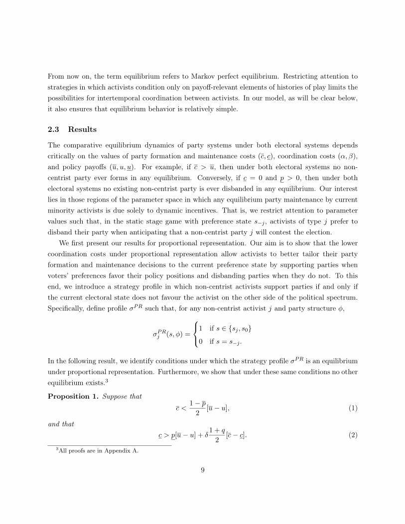
Proposition 1. Suppose that

c <1− p

2[u− u], (1)

and thatc > p[u− u] + δ

1 + q

2[c− c]. (2)

3All proofs are in Appendix A.

9

Then σPR is the unique Markov perfect equilibrium under proportional representation.

Condition (1) ensures that a non-centrist activist j always supports a party in sj and s0, sothat the only remaining question is whether or not the activist will support a party in s−j . Notethat under condition (2), we have that p[u− u]− c < 0, so in the stage game with preference states−j , activist j prefers disbanding an existing party to maintaining it. However, maintaining anexisting party in s−j has an associated option value realized in sj and s0, which is derived from thecost savings for supporting a party in those states. Condition (2) ensures that under proportionalrepresentation, the immediate cost savings from disbanding an existing party dominates the optionvalue of supporting it through an unfavourable election. Conditions (1) and (2) uniquely pin downthe optimal party formation and maintenance decisions of both non-centrist activists, so that noother equilibrium can exist. Also, note that while the equilibrium σPR is in symmetric strategies,we impose no ex ante symmetry restriction on equilibria.

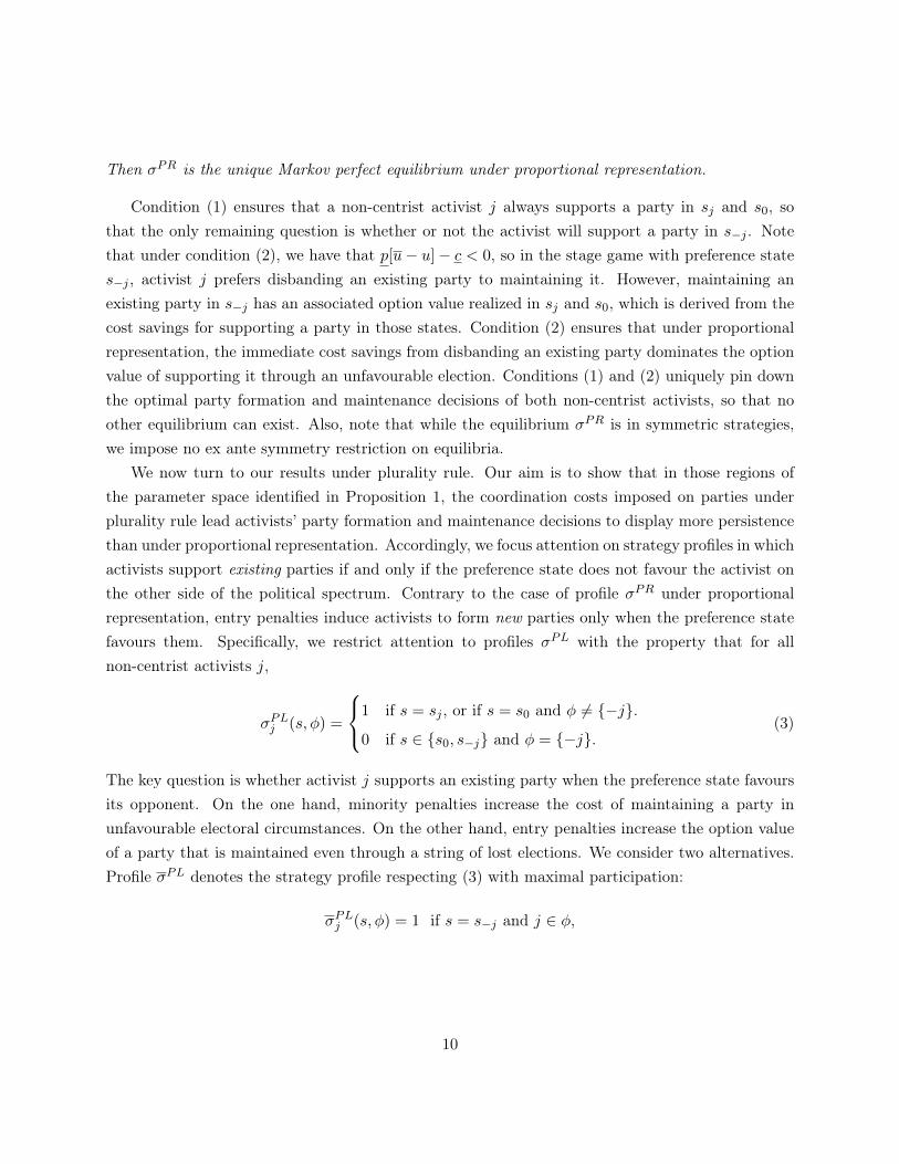
We now turn to our results under plurality rule. Our aim is to show that in those regions ofthe parameter space identified in Proposition 1, the coordination costs imposed on parties underplurality rule lead activists’ party formation and maintenance decisions to display more persistencethan under proportional representation. Accordingly, we focus attention on strategy profiles in whichactivists support existing parties if and only if the preference state does not favour the activist onthe other side of the political spectrum. Contrary to the case of profile σPR under proportionalrepresentation, entry penalties induce activists to form new parties only when the preference statefavours them. Specifically, we restrict attention to profiles σPL with the property that for allnon-centrist activists j,

σPLj (s, φ) =

1 if s = sj , or if s = s0 and φ 6= {−j}.

0 if s ∈ {s0, s−j} and φ = {−j}.(3)

The key question is whether activist j supports an existing party when the preference state favoursits opponent. On the one hand, minority penalties increase the cost of maintaining a party inunfavourable electoral circumstances. On the other hand, entry penalties increase the option valueof a party that is maintained even through a string of lost elections. We consider two alternatives.Profile σPL denotes the strategy profile respecting (3) with maximal participation:

σPLj (s, φ) = 1 if s = s−j and j ∈ φ,

10

while profile σPL denotes the strategy profile respecting (3) with minimal participation:

σPLj (s, φ) = 0 if s = s−j and j ∈ φ.

In the following result, we identify conditions under which σPL and σPL are equilibria underplurality rule.4 These conditions will depend on the entry penalty β being bounded above and below.These upper and lower bounds, denoted β and β respectively, are functions of all the parameters ofthe problem except the minority penalty α, and they are derived in Appendix A.

Proposition 2. Suppose that (1) and (2) hold and that β ∈ (β, β). Then there exist α, α ∈ [0, p−β]

such that σ is a Markov perfect equilibrium whenever α > α and σ is a Markov perfect equilibriumwhenever α < α. Furthermore, α ≥ α.

Our dynamic model provides no robust cross-sectional predictions on the number of partiesunder different electoral systems. In any given election under proportional representation, therecould be either two or three parties competing (under σPR). Under plurality, our model allowsfor the standard Duverger prediction of a two-party system (under σPL), although the identitiesof the parties change over time as voters’ preferences evolve, but it also allows for a non-Duvergerequilibrium in which three parties are always present (under σPL). However, our model does providea robust dynamic prediction: there is greater variation in the number of active parties in equilibriumσPR under proportional representation than under either of the equilibria σPL and σPL that weidentify under plurality. To see this, first note that there is no variation in the number of partiesunder σPL as three parties contest all elections. To compare σPR and σPL, note that under bothequilibria, a transition from sj to s−j leads to the exit of the party representing activist j and theentry of the party representing activist −j. However, for other transitions in preference states, σPR

generates more variability in the number of parties. A transition from sj to s0 leads to the entry ofparty −j under σPR but not under σPL, while a transition from s0 to sj always leads to the exit ofparty −j under σPR. This party need not be active in this state under σPL, in which case no exitcan occur.

Although preference states are drawn independently across periods, party structures under plu-rality are history-dependent while party structures under proportional representation are not. UnderσPR, the probability that a party representing activist j contests any election is 1+q

2 (the proba-bility that the preference state is either sj or s0) which does not depend on the realization of pastpreference states or party structures. Under plurality, party structures are fully persistent in the

4Activist j’s actions are not yet specified only if the preference state is s−j and no activists supported partiesin the previous elections (i.e., φt = ∅). These histories only occur off the equilibrium path, and the details are inAppendix A.

11

equilibrium σPL, as no party ever exits. In the equilibrium σPR, the probability that a party rep-resenting activist j contests an election at time t depends on whether or not this party contestedan election at time t− 1. Specifically, if j ∈ φt−1, then party j contests the election at time t withprobability 1+q

2 , the probability that the preference state is either sj or s0. On the other hand, ifj /∈ φt−1, then it contests the election with probability 1−q

2 , the probability that the preference statetransitions to sj .

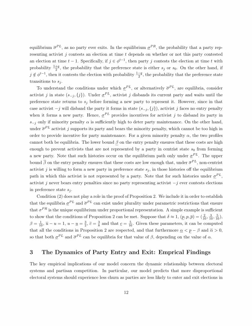
To understand the conditions under which σPL, or alternatively σPL, are equilibria, consideractivist j in state (s−j , {j}). Under σPL, activist j disbands its current party and waits until thepreference state returns to sj before forming a new party to represent it. However, since in thatcase activist −j will disband the party it forms in state (s−j , {j}), activist j faces no entry penaltywhen it forms a new party. Hence, σPL provides incentives for activist j to disband its party ins−j only if minority penalty α is sufficiently high to deter party maintenance. On the other hand,under σPL activist j supports its party and bears the minority penalty, which cannot be too high inorder to provide incentive for party maintenance. For a given minority penalty α, the two profilescannot both be equilibria. The lower bound β on the entry penalty ensures that these costs are highenough to prevent activists that are not represented by a party in centrist state s0 from forminga new party. Note that such histories occur on the equilibrium path only under σPL. The upperbound β on the entry penalty ensures that these costs are low enough that, under σPL, non-centristactivist j is willing to form a new party in preference state sj , in those histories off the equilibriumpath in which this activist is not represented by a party. Note that for such histories under σPL,activist j never bears entry penalties since no party representing activist −j ever contests electionsin preference state sj .

Condition (2) does not play a role in the proof of Proposition 2. We include it in order to establishthat the equilibria σPL and σPL can exist under plurality under parametric restrictions that ensurethat σPR is the unique equilibrium under proportional representation. A simple example is sufficientto show that the conditions of Proposition 2 can be met. Suppose that δ ≈ 1, (p, p, p) = ( 2

10 ,310 ,

510),

β = 110 , u− u = 1, u− u = 3

2 , c = 38 and that c = 5

16 . Given these parameters, it can be computedthat all the conditions in Proposition 2 are respected, and that furthermore α < p− β and α > 0,so that both σPL and σPL can be equilibria for that value of β, depending on the value of α.

3 The Dynamics of Party Entry and Exit: Emprical Findings

The key empirical implications of our model concern the dynamic relationship between electoralsystems and partisan competition. In particular, our model predicts that more disproportionalelectoral systems should experience less churn as parties are less likely to enter and exit elections in

12

these systems. To test these predictions, we use the Constituency-Level Elections (CLE) Dataset(Brancati (accessed 2013)), which contains information on the vote shares and seat shares of allpolitical parties that participated in a broad sample of national democratic elections. Our empiricalanalysis consists of estimating the relationship between the disproportionality of an electoral systemand the dynamics of its party system through party entries and exits. We do not ascribe a causalinterpretation to any portion of our empirical anlysis as our aim is simply to provide robust evidencethat is consistent with the central predictions of our model.

There are two main measurement issues that we must address in order to conduct our analysis.First, we need a concise measure of the proportionality of an electoral system, which is determinedby institutional characteristics such as electoral laws in a potentially complex manner. Second, weneed an appropriate measure of party entry and exit. A key difficulty here is that electoral systemsdiffer in their number of districts with more proportional systems having less districts on averagethan plurality systems, and parties may be active in some districts and not others. This can be thecase if, for instance, a party’s support is regional in nature. Alternatively, a successful entry in afew districts may be a launching pad for a new national party.

To address the first issue, we follow Taagepera and Shugart (1989) and measure the proportion-ality of an electoral system by its effective district magnitude, which is defined as the total numberof legislators directly elected in electoral districts divided by the total number of electoral districts.5

Because this measure is purely determined by a country’s electoral institutions, it is our preferredmeasure of proportionality. Furthermore, it is well established that more proportional electoralsystems are associated with higher effective district magnitudes.

We supplement our analysis with an additional, alternative measure of the proportionality ofan electoral system by using the least squares index of Gallagher (1991). This index, which hasbeen used in empirical analyses of electoral systems, is a measure of the difference between parties’vote and seat shares in a given election.6 In perfectly proportional electoral systems, parties’ seatshares should be identical to their vote shares, while in less proportional systems front-runningparties typically have seat shares exceeding their vote shares and lagging parties have seat shareswell below their share of the votes. Formally, for a given election e in a given country c with J totalparties, let pjce be the vote share that party j receives, and let sjce be the seat share that party j

5Effective district magnitude can differ from average district magnitude, which is defined as the total number oflegislative seats divided by the number of electoral districts. Taagepera and Shugart (1989) argue that effective districtmagnitude is the superior measure of the proportionality of an electoral system. To the extent that a legislature doesnot feature at-large seats, these measures are identical.

6See also Lijphart (1994) and Taagepera and Grofman (2003).

13

wins in the legislature. Then the disproportionality index for this election is given by

gce =

√√√√1

2

J∑j=1

(pjce − sjce)2 (4)

where gce is an index that ranges from 0 to 1 with increasing values corresponding to more dispro-portional elections. Because disproportionality is a property of the electoral institutions of country,it should should not vary either by electoral district or by election. Hence, we aggregate districtelectoral outcomes and compute the disproportionality index at the national level. Furthermore, weaverage the disproportionality index over all elections for a different country, i.e.,

Gc =1

Ec

Ec∑e=1

gce (5)

where Ec is the total number of elections that we observe for country c. Gc constitutes an alternativemeasure of the (dis)proportionality of the electoral system of country c. Since the numbers of partiesactive in a given country enter into the the determination of the disproportionality index Gc, it isgenerally agreed that measures of district magnitude are cleaner proxies for electoral systems thandisproportionality indices (see, for example, Ordeshook and Shvetsova (1994)). However, we includespecifications with the disproportionality index to highlight the strength or our results.

To address the issue of measuring party entry and exit, we proceed as follows. For any election ein country c, we denote the number of electoral districts Dce, where district d contributes a fractionσdce of the total seats in the national legislature. A party is said to have entered in district d inelection e if its vote share in that district in e−1 was less than 0.05 and its vote share in that districtin e was greater than 0.05. Party exit is defined similarly.7 Let ndce and xdce represent, respectively,the total number of entering and exiting parties in district d during election e in country c. Thetotal number of entries Nce in a given election is obtained by summing over all districts as

Nce =

Dce∑d=1

ndce · σdce, (6)

and the total number of exits Xce can be defined similarly as

Xce =

Dce∑d=1

xdce · σdce. (7)

7As a robustness check, we replicated our analysis replacing the 0.05 threshold for entry and exit with 0.01, 0.02and 0.10 and obtained similar results.

14

We weigh the number of entries in each district by that district’s size in order to correct for thevariability in the number of electoral districts across electoral systems. For example, Israel, whichis considered to have an electoral system that is almost perfectly proportional, has a single electoraldistrict, so one entry is recorded if a new party collects a share of 0.05 of votes at the nationallevel. The United Kingdom, on the other hand, has all legislators elected by plurality rule in oversix hundred electoral districts, so that one entry is recorded if a new party collects a share 0.05

of votes in every district. The emergence of a regional party that collects the threshold share ofvotes in, say, half of the country’s districts, would be recorded as half an entry. In the absence ofweighing district-level party entries and exits, the variability in party structures in plurality rulesystems would be dramatically overstated. Finally, the total net party movements in an election(i.e., the total amount of partisan churn), Mce, is simply defined as the sum of entries and exits as

Mce = Nce +Xce.

We construct these variables from the CLE, which contains detailed information on the identitiesof all parties that participated in a large number of elections in many countries since 1945.8 Inparticular, the CLE documents the number of votes that each party received in each district of agiven election and the number of legislative seats that they were awarded. With this information, itis straightforward to construct the measures described above. In Figure 1, we plot both the effectivedistrict magnitude and the average disproportionality index for the countries in our sample.9 Asis well known, countries with lower effective magnitudes are associated to higher disproportionalityscores. Because all countries do not hold elections at the same frequency (and several countrieswere formed or ceased to exist since 1945) our data set constitutes an unbalanced panel.

In Table 1, we present traditional, static tests of Duverger’s Law and explore the relation-ship between the proportionality of electoral systems and the number of parties that compete inelections.10 When measuring proportionality with effective district magnitude, we uncover no mean-ingful relationship between proportionality and the number of parties that compete in elections. Allcoefficients in the first four columns are both small and statistically indistinguishable from zero.

8The CLE unfortunately does not contain data on all democratic elections since 1945. Indeed, no single sourcedoes. We use only those elections contained in the CLE for our analysis and do not supplement our dataset with datafrom other sources in order to maintin consistent reporting. We replicated our analysis using a similar (thought notidentical) sample of elections from the Constituence Level Elections Archive (CLEA) data set and obtained similarresults. We report results using the CLE because this is the dataset that has been primarily used to constructdisproportionality indices (Gallagher and Mitchell (2005)).

9All tables are in Appendix B.10The number of competing parties is computed in a similar manner to the numbers of entries and exits. That

is, any party that receives a vote share over 0.05 in any election is counted. Our results are robust to alternativethresholds of 0.01, 0.02 and 0.10.

15

When we use the disproportionality index as an alternative representation of electoral systems, wefind a weakly negative relationship between disproportionality and the number of competing par-ties, which is consistent with our model (thought not dispositive). However, this correlation is notstatistically significant.11 This weak evidence in favor of the static version of Duverger’s Law is notconsiderably strengthened when we add additional control variables in specifications (6) through(8); the basic finding of a negative but statistically insignificant relationship persists.12

In Table 2, we present our main empirical results, which explore the dynamic relationshipbetween the proportionality of electoral systems and the number of parties that compete in elections.In each set of four columns, we specify total entries, exits and net movements as the dependentvariable respectively and the effective district magnitude (scaled by a factor of 100) as the primaryindependent variable. The coefficient of interest on this variable is predicted to be positive by ourmodel. For each dependent variable, we estimate four regressions, each of which includes differentsets of control variables. In all regressions, we specify all continuous variables in logarithms. Bydoing so, our parameter estimates are scale invariant. This ensures that electoral systems with manyparties (which tend to be more proportional, per the static results) do not simply exhibit a largeamount of partisan churn by construction. Rather, any such relationship between proportionalityand partisan churn should be interpreted as independent of the total number of parties. Becauseelections may feature zero entries or exits, we transform all continuous variables x as log (1 + x)

in order to conserve data. Because the effective district magnitude does not vary within countrieswith fixed electoral systems by construction, we cluster our standard errors at the country level toaccount for this induced multicollinearity.

In the first specification, we include no control variables. Consistent with our model, we esti-mate positive relationship between effective district magnitude and all three dependent variables.More proportional electoral systems feature greater amounts of both entry and exit of parties. Inthe second specification, we include dummies for each decade in order to absorb slowly varyingglobal determinants of partisan political activity,13 and we include regional dummies for Europeancountries, African countries, and former republics of the USSR in order to absorb any regional deter-minants of political activity. Estimates of our coefficients of interest are unchanged and statisticallysignificant at least at the 99% level. In the third specification, we flexibly control for the number ofdistricts by including sixth order polynomials in Dce and logDce.14 Because Dce explicitly enters

11The specification in column (5) essentially reproduces the correlations in Table 3.4 of Lijphart (1994).12Note that in specification (8), which contains the most control variables, the coefficient on disproportionality is

significant at the 90% level.13Our decade dummies are defined for the periods 1940-49, 1950-59, ... , 2000-2009. We replicated our analysis

defining decade dummies for all possible periods (e.g., 1948-1957, ...) and obtained results that were statisticallyindistinguishable from those presented.

14As a robustness check, we replicated our analysis with polynomials of all orders up to 10 in Dce and logDce and

16

into our computation of entries and exits in equations (6) and (7), conditioning our regressionson the number of districts ensures that the coefficients of interest that we estimate are not simplymechanically determined by variation in this Dce. Indeed, our coefficient estimates in specification(3) are unchanged and statistically significant at the 99% level. Finally, in the fourth specification,we flexibly control for the number of competing parties by including sixth order polynomials inJce and log Jce. This ensures that we do not merely estimate a mechanical relationship betweenthe number of parties and partisan churn. Our coefficient estimates are once again unchanged andstatistically significant at the 99% level.

As we specify successively richer sets of controls, we are able to explain an increasing amount ofthe variation in partisan entry, exit and churn (note the increases in R2). However, our estimates ofthe relationship between proportionality and these variables is effectively unchanged. We interpretthis as robust evidence that is consistent with the dynamic predictions of our model. In orderto explore the extent to which these findings rely on the use of effective district magnitude as ameasure of proportionality, we respecify proportionality using the average disproportionality indexGc of a country and present coefficient estimates in Table 3. Consistent with the predictions of ourmodel, we find a robust negative relationships between disproportionality and partisan churn. Theserelationships persist as we add successively richer sets of control variables, although the estimatedtcoefficients are not as stable across specifications as our previous results.15

4 Conclusion

This paper presents a novel dynamic reinterpretation of Duverger’s Law. We construct a minimalbut transparent dynamic model that establishes that (i) static Duverger predictions on the compar-ative number of parties under plurality rule and proportional representation can be reversed whenintertemporal incentives are taken into account and that (ii) a unique dynamic prediction can berecovered if we focus our attention on the comparative variation in the number of parties over timeacross electoral systems. We finds robust empirical support in favor of the latter prediction.

Since party formation and maintenance decisions are typically made on a national level, thedynamic predictions of our model can only be verified appropriately with cross-country electionsdata. Further, since electoral systems rarely change within countries, this hinders any attempt toattribute a causal effect of electoral systems on the evolution of the number of national parties.

obtained qualitatively similar negative and statistically significant estimates of our coefficients of interest at the 99%level.

15As a robustness check, we reestimated all regressions in table 3 by specifying proportionality as the dispropor-tionality index of the first election for each country in our sample (as opposed to the average value of over elections).In doing so we obtained qualitatively similar and statistically significant results.

17

We consider the time-series correlations uncovered in this paper sufficiently novel, interesting androbust that the lack of a causal interpretation does not present a critical concern. However, we makea broader contribution in that we point to the interest of studying the comparative intertemporalproperties of electoral systems. In future work, related questions along these lines may be amenableto causal inference as, for example, the study of the comparative importance of strategic voting inFujiwara (2011) allowed causal claims about political forces leading to the cross-country predictionson the number of parties.

References

Benoit, K., 2002. The endogeneity problem in electoral studies: a critical re-examination of du-verger’s mechanical effect. Electoral Studies 21 (1), 35–46.

Benoit, K., 2006. Duverger’s law and the study of electoral systems. French Politics 4 (1), 69–83.

Blais, A., Carty, R. K., 1991. The psychological impact of electoral laws: measuring duverger’selusive factor. British Journal of Political Science, 79–93.

Brancati, D., accessed 2013. Global Elections Dataset. New York: Global Elections Database,http://www.globalelectionsdatabase.com.

Chhibber, P., Kollman, K., 1998. Party aggregation and the number of parties in india and theunited states. American Political Science Review, 329–342.

Chhibber, P., Murali, G., 2006. Duvergerian dynamics in the indian states federalism and thenumber of parties in the state assembly elections. Party Politics 12 (1), 5–34.

Cox, G. W., 1997. Making votes count: strategic coordination in the world’s electoral systems.Vol. 7. Cambridge Univ Press.

Diwakar, R., 2007. Duverger’s law and the size of the indian party system. Party Politics 13 (5),539–561.

Duverger, M., 1951. Les partis politiques. Armand Colin.

Faravelli, M., Sanchez-Pages, S., 2012. (don’t) make my vote count.

Feddersen, T. J., 1992. A voting model implying duverger’s law and positive turnout. Americanjournal of political science, 938–962.

18

Fey, M., 1997. Stability and coordination in duverger’s law: A formal model of preelection polls andstrategic voting. American Political Science Review, 135–147.

Fujiwara, T., 2011. A regression discontinuity test of strategic voting and duverger’s law. QuarterlyJournal of Political Science 6 (3-4), 197–233.

Gaines, B. J., 1999. Duverger’s law and the meaning of canadian exceptionalism. ComparativePolitical Studies 32 (7), 835–861.

Gallagher, M., 1991. Proportionality, disproportionality and electoral systems. Electoral studies10 (1), 33–51.

Gallagher, M., Mitchell, P., 2005. The politics of electoral systems. Cambridge Univ Press.

Herrera, H., Morelli, M., Palfrey, T. R., 2012. Turnout and power sharing.

Lijphart, A., 1994. Electoral systems and party systems: A study of twenty-seven democracies,1945-1990. Oxford University Press.

Morelli, M., 2004. Party formation and policy outcomes under different electoral systems. TheReview of Economic Studies 71 (3), 829–853.

Neto, O. A., Cox, G. W., 1997. Electoral institutions, cleavage structures, and the number of parties.American Journal of Political Science, 149–174.

Ordeshook, P. C., Shvetsova, O. V., 1994. Ethnic heterogeneity, district magnitude, and the numberof parties. American journal of political science, 100–123.

Palfrey, T., 1989. A mathematical proof of duverger’s law. In: Ordeshook, P. C. (Ed.), Models ofstrategic choice in politics. University of Michigan Press.

Reed, S. R., 2001. Duverger’s law is working in italy. Comparative Political Studies 34 (3), 312–327.

Riker, W. H., 1982. The two-party system and duverger’s law: An essay on the history of politicalscience. The American Political Science Review, 753–766.

Shugart, M. S., 2005. Comparative electoral systems research: the maturation of a field and newchallenges ahead. In: Gallagher, M., Mitchell, P. (Eds.), The politics of electoral systems. Cam-bridge Univiversity Press.

Taagepera, R., Grofman, B., 2003. Mapping the indices of seats–votes disproportionality and inter-election volatility. Party Politics 9 (6), 659–677.

19

Taagepera, R., Shugart, M. S., 1989. Seats and votes: The effects and determinants of electoralsystems. Yale University Press.

A Appendix: Proofs

Proof of Proposition 1. Note that (1) implies that under proportional representation, forming (ormaintaining, since c > c) a party is uniquely stage optimal in preference state s0 for party j,irrespective of whether activist −j is represented by a party. Also, since p > 1

3 , (1) implies that c ≤p[u−u], so that forming (or maintaining, since c > c) a party is uniquely stage optimal in preferencestate sj for party j, irrespective of whether activist −j is represented by a party. Finally, since c > c,it follows that, for any state (s, φ) and any equilibrium σ∗, Vj(s, φ ∪ {j};σ∗) ≥ Vj(s, φ;σ∗). Hence,in any equilibrium under proportional representation, it must be that σ∗j (s, φ) = 1 for all statessuch that s ∈ {s0, sj}.

It remains only to determine activists’ equilibrium actions in preference state s−j . Fix anequilibrium σ∗ and consider a state (s−j , φ) such that j ∈ φ. If activist j disbands its party, itspayoff is

Vj(s−j , φ;σ∗) = (1− p)u+ pu+ δEVj(s′, {−j};σ∗)

If instead activist j maintains its party, let V d(s−j , φ;σ∗) be its payoff. We have that

V dj (s−j , φ;σ∗) = pu+ pu+ pu− c+ δEVj(s′, {−j, j};σ∗).

By our results from above, we have that, for any s ∈ {s0, sj},

Vj(s, {−j};σ∗) = Vj(s, {−j, j};σ∗)− [c− c],

so that Vj(s−j , φ;σ∗) > V dj (s−j , φ;σ∗) if and only if (2) holds. Note that (2) also implies that

in state (s−j , φ) such that j /∈ φ, activist j strictly prefers not to form a party. Hence, for anyequilibrium σ∗ under proportional representation, we have that σ∗ = σPR.

Proof of Proposition 2. Define β and β such that

β[u− u] ≡ 1

1− δq

[1− p

2[u− u]− c

]−

1− δ 1+q21− δq

[c− c] , and

β[u− u] ≡ p[u− u]− c+δ

1− δ

[1− p

2[u− u]− c

]+δ(1− q)

1− δp− p

2[u− u].

20

Fix any equilibrium σ∗. First, note that since β ≥ 0, under plurality as under proportionalrepresentation, (1) implies that maintaining an existing party is uniquely stage optimal in preferencestate s0 for activist j, irrespective of whether activist −j is represented by a party. Hence, by thearguments in the proof of Proposition 1, σ∗j (s0, φ) = 1 whenever j ∈ φ. Second, since α ≥ 0, (1)also implies that σ∗j (sj , φ) = 1 whenever j ∈ φ. Third, since no new party faces entry penalty βfollowing entry when φ = ∅, (1) also ensures that σ∗j (s, ∅) = 1 is uniquely optimal when s ∈ {s0, sj}.

Now consider state (s0, {−j}) and equilibrium σ∗. If activist j does not form a party, its payoffis

1 + p

2u+

1− p2

u+ δEVj(s′, {−j};σ∗),

while if activist j forms a party, its payoff is(1− p

2− β

)u+ pu+

(1− p

2+ β

)u− c+ δEVj(s′, {−j, j};σ∗).

Hence, activist j does not form a party if and only if

c−[

1− p2

[u− u]− β[u− u]

]≥ δE

[Vj(s

′, {−j, j};σ∗)− Vj(s′, {−j};σ∗)]

≡ δE∆Vj(s′;σ∗) (8)

Consider state (s−j , φ) such that j ∈ φ and such that σ∗−j(s−j , φ) = 1. If activist j maintainsits party, its payoff is

(p− α+ βI−j /∈φ)u+ pu+ (p+ α− βI−j /∈φ)u− c+ δEVj(s′, {−j, j};σ∗),

while if activist j disbands its party, its payoff is

(1− p)u+ pu+ δEVj(s′, {−j};σ∗).

Hence, under profile σPL, it must be that

c− p[u− u] + (α− β)[u− u] ≥ δE∆Vj(s′;σPL), (9)

while under profile σPL, it must be that

c− p[u− u] + α[u− u] ≤ δE∆Vj(s′;σPL). (10)

Fix a state (sj , φ) such that j /∈ φ. Under σPL, (1) ensures that the stage payoffs of activist j

21

are strictly positive when it forms a party, so that, by an argument in the proof of Proposition 1,σPL(sj , φ) = 1 is optimal. Under σPL, activist j forms a party in state (sj , φ) with j /∈ φ if andonly if

p[u− u]− c+ (α− β)[u− u] ≥ −δE∆Vj(s′;σPL). (11)

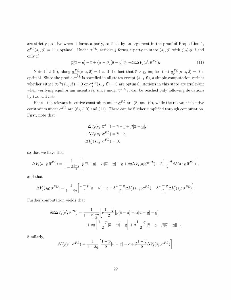
Note that (9), along σPL−j (s−j , ∅) = 1 and the fact that c > c, implies that σPLj (s−j , ∅) = 0 isoptimal. Since the profile σPL is specified in all states except (s−j , ∅), a simple computation verifieswhether either σPLj (s−j , ∅) = 0 or σPLj (s−j , ∅) = 0 are optimal. Actions in this state are irrelevantwhen verifying equilibrium incentives, since under σPL it can be reached only following deviationsby two activists.

Hence, the relevant incentive constraints under σPL are (8) and (9), while the relevant incentiveconstraints under σPL are (8), (10) and (11). These can be further simplified through computation.First, note that

∆Vj(sj ;σPL) = c− c+ β[u− u],

∆Vj(sj ;σPL) = c− c,

∆Vj(s−j ;σPL) = 0,

so that we have that

∆Vj(s−j ;σPL) =

1

1− δ 1−q2

[p[u− u]− α[u− u]− c+ δq∆Vj(s0;σ

PL) + δ1− q

2∆Vj(sj ;σ

PL)

],

and that

∆Vj(s0;σPL) =

1

1− δq

[1− p

2[u− u]− c+ δ

1− q2

∆Vj(s−j ;σPL) + δ

1− q2

∆Vj(sj ;σPL)

].

Further computation yields that

δE∆Vj(s′;σPL) =

1

1− δ 1+q2

[δ

1− q2

[p[u− u]− α[u− u]− c

]+ δq

[1− p

2[u− u]− c

]+ δ

1− q2

[c− c+ β[u− u]]

].

Similarly,

∆Vj(s0;σPL) =

1

1− δq

[1− p

2[u− u]− c+ δ

1− q2

∆Vj(sj ;σPL)

],

22

and further computation yields that

δE∆Vj(s′;σPL) =

1

1− δq

[δq

[1− p

2[u− u]− c

]+ δ

1− q2

[c− c]].

Evaluated at σPL, (8) can be rewritten as

β[u− u] ≥1− δ 1−q21− δq

[1− p

2[u− u]− c

]− [c− c] +

δ 1−q21− δq

[p[u− u]− α[u− u]− c

], (12)

while evaluated at σPL, it can be rewritten as

β[u− u] ≥ 1

1− δq

[1− p

2[u− u]− c

]−

1− δ 1+q21− δq

[c− c] . (13)

A straightforward computation verifies that, for any α, the righthand side of (13) is strictly largerthan the righthand side of (12), so that (12) holds whenever (13) holds.

Also, (9) can be rewritten as

α[u− u] ≥ p[u− u]− c+ β[u− u] +1

1− δq

[δq

[1− p

2[u− u]− c

]+ δ

1− q2

[c− c]], (14)

while (10) can be rewritten as

α[u− u] ≤ p[u− u]− c+1

1− δq

[δq

[1− p

2[u− u]− c

]+ δ

1− q2

[c− c+ β[u− u]]

]. (15)

Finally, since the righthand side of (11) is increasing in α, it can be shown by computation to holdfor all α if and only if

β[u− u] ≤ p[u− u]− c+δ

1− δ

[1− p

2[u− u]− c

]+δ(1− q)

1− δp− p

2[u− u], (16)

That (13) holds follows since β ≥ β, and that (16) holds follows since β ≤ β. Hence, conditions(13) and (14) are sufficient for σPL to be an equilibrium, while (13), (15) and (16) are sufficient forσPL to be an equilibrium. Let α̌ be the unique value of α such that (14) holds as an equality anddefine α = max{min{p − β, α̌}, 0}. Similarly, let α̂ be the unique value of α such that (15) holdsas an equality and define α = min{max{0, α̂}, p − β}. Hence, given any β satisfying (13), σPL isan equilibrium if α > α, while σPL is an equilibrium if α < α. These are sufficient conditions only,since our definition of α and α embeds the cases when these equilibria fails to exits. Furthermore,

23

(14) and (15) imply that α ≥ α, where the inequality is strict whenever α, α ∈ (0, p− β).

B Appendix: Tables and Figures

Figure 1: Proportionality and Effective District Magnitude

AlbaniaAustralia

Austria

Belg.

Bermuda

BoliviaBos.-Herz.

Botswana

Bulgaria

Can.

C. Rica

Croatia

Cyprus

Czech Rep.

Czechoslovakia

Estonia

Finland

France

Germany

Greece

Hungary

Iceland

Indonesia

Ireland

Israel

ItalyLatvia

Lith.

Lux.

. Malaysia

Malta

MauritiusMexico

Moldova

Neth.

N. Zeal.

Niger

Norw.

Poland

Portugal

Rom.

Russia

Slovakia

Slovenia

S. Africa

Spain

Sweden

Switz.

Trin. & Tob.

Turkey

UKUS

Ven.

W. Germany

.1.2

.3.4

Ave

rage

Gal

lagh

er D

ispr

opor

tiona

lity

Inde

x

50 100 150Effective District Magnitude

Notes: Both axes are in log scale. All variables are constructed from the Constituency-Level Elections (CLE) Dataset.

24

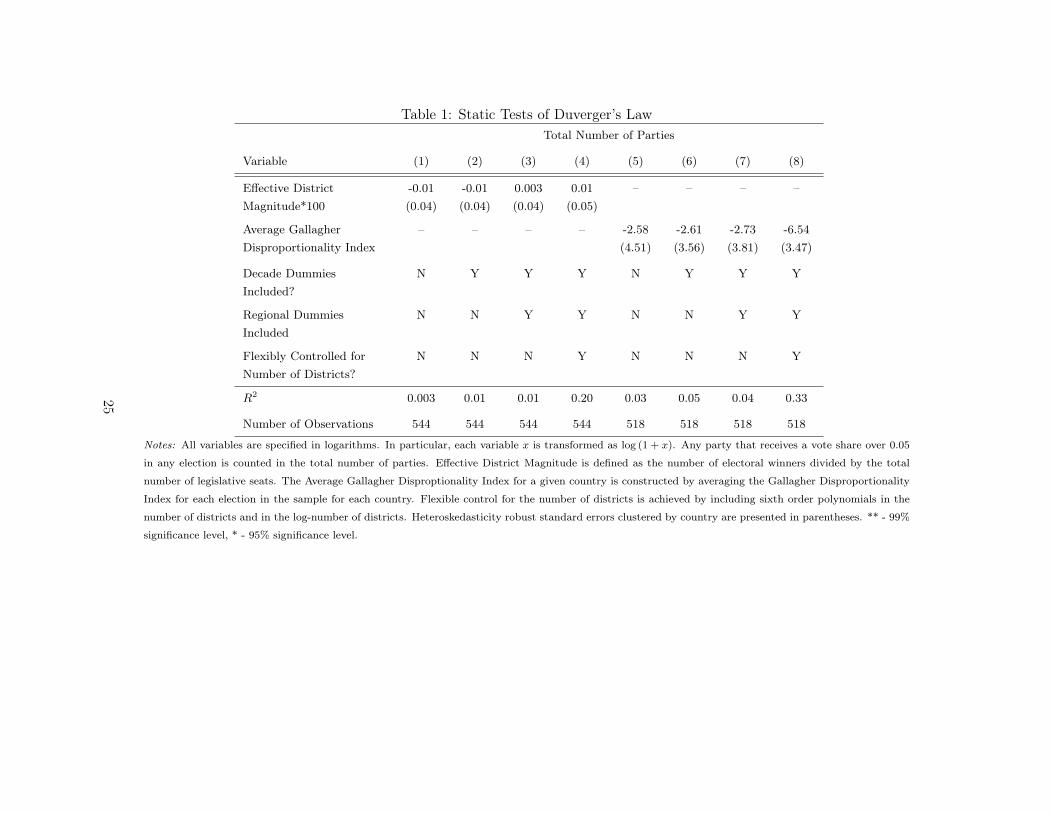
Table 1: Static Tests of Duverger’s LawTotal Number of Parties

Variable (1) (2) (3) (4) (5) (6) (7) (8)

Effective DistrictMagnitude*100

-0.01(0.04)

-0.01(0.04)

0.003(0.04)

0.01(0.05)

– – – –

Average GallagherDisproportionality Index

– – – – -2.58(4.51)

-2.61(3.56)

-2.73(3.81)

-6.54(3.47)

Decade DummiesIncluded?

N Y Y Y N Y Y Y

Regional DummiesIncluded

N N Y Y N N Y Y

Flexibly Controlled forNumber of Districts?

N N N Y N N N Y

R2 0.003 0.01 0.01 0.20 0.03 0.05 0.04 0.33

Number of Observations 544 544 544 544 518 518 518 518

Notes: All variables are specified in logarithms. In particular, each variable x is transformed as log (1 + x). Any party that receives a vote share over 0.05

in any election is counted in the total number of parties. Effective District Magnitude is defined as the number of electoral winners divided by the total

number of legislative seats. The Average Gallagher Disproptionality Index for a given country is constructed by averaging the Gallagher Disproportionality

Index for each election in the sample for each country. Flexible control for the number of districts is achieved by including sixth order polynomials in the

number of districts and in the log-number of districts. Heteroskedasticity robust standard errors clustered by country are presented in parentheses. ** - 99%

significance level, * - 95% significance level.

25

Table 2: Dynamic Tests of Duverger’s Law: Effective District MagnitudeTotal Entries Total Exits Total Net Movements

Variable (1) (2) (3) (4) (1) (2) (3) (4) (1) (2) (3) (4)

Effective DistrictMagnitude*100

0.06**(0.01)

0.05**(0.01)

0.06**(0.01)

0.06**(0.01)

0.06**(0.01)

0.05**(0.01)

0.06**(0.01)

0.06**(0.01)

0.09**(0.02)

0.09**(0.01)

0.10**(0.01)

0.10**(0.01)

Decade DummiesIncluded?

N Y Y Y N Y Y Y N Y Y Y

Decade and RegionalDummies Included?

N Y Y Y N Y Y Y N Y Y Y

Flexibly Controlled forNumber of Districts?

N N Y Y N N Y Y N N Y Y

Flexibly Controlled forNumber of Parties?

N N N Y N N N Y N N N Y

R2 0.08 0.22 0.23 0.32 0.06 0.18 0.23 0.30 0.10 0.22 0.26 0.32

Number ofObservations

544 544 544 544 544 544 544 544 544 544 544 544

Notes: All variables are specified in logarithms. In particular, each variable x is transformed as log (1 + x). Entries and exits are computed according to

equations (6) and (7). Total net movements = entries + exits. Flexible control for the number of districts and parties is achieved by including sixth order

polynomials in those variables and in the log of those variables. Heteroskedasticity robust standard errors clustered by country are presented in parentheses.

** - 99% significance level, * - 95% significance level.

26

Table 3: Dynamic Tests of Duverger’s Law: Gallagher IndexTotal Entries Total Exits Total Net Movements

Variable (1) (2) (3) (4) (1) (2) (3) (4) (1) (2) (3) (4)

Average GallagherDisproportionalityIndex

-0.74*(0.33)

-0.79*(0.34)

-1.05**(0.28)

-1.73**(0.60)

-0.54(0.40)

-0.65(0.35)

-0.89**(0.28)

-1.17*(0.64)

-0.95*(0.48)

-1.10*(0.46)

-1.40**(0.37)

-2.13**(0.82)

Decade DummiesIncluded?

N Y Y Y N Y Y Y N Y Y Y

Decade and RegionalDummies Included?

N Y Y Y N Y Y Y N Y Y Y

Flexibly Controlled forNumber of Districts?

N N Y Y N N Y Y N N Y Y

Flexibly Controlled forNumber of Parties?

N N N Y N N N Y N N N Y

R2 0.01 0.16 0.18 0.27 0.01 0.13 0.18 0.25 0.01 0.16 0.19 0.25

Number ofObservations

518 518 518 518 518 518 518 518 518 518 518 518

Notes: All variables are specified in logarithms. In particular, each variable x is transformed as log (1 + x). Entries and exits are computed according to

equations (6) and (7). Total net movements = entries + exits. Flexible control for the number of districts and parties is achieved by including sixth order

polynomials in those variables and in the log of those variables. Heteroskedasticity robust standard errors clustered by country are presented in parentheses.

** - 99% significance level, * - 95% significance level.

27