a dynamic model of female labor force participation rate ... · a dynamic model of female labor...

JOURNAL OF ECONOMIC DEVELOPMENT 81 Volume 39, Number 3, September 2014

A DYNAMIC MODEL OF FEMALE LABOR FORCE PARTICIPATION

RATE AND HUMAN CAPITAL INVESTMENT

RADEK SZULGA*

Carleton College, U.S.A.

This paper develops a dynamic model of human capital investment and labor participation. The main focus is on the fact that women’s labor force participation rate is U-shaped over the course of development. We also analyze the behavior of the relative education levels of men and women, the education levels of women in the labor force and outside of it, and the magnitude and sign of income and wage effects. The underlying assumption of the model is the existence of economies of scope in the traditional sector of the economy. This creates a tradeoff between remaining in traditional production where farm work and child rearing can be undertaken simultaneously, and moving to modern production where income is potentially higher. Keywords: Female Labor Force Participation Rate, Human Capital, Economic Growth JEL classification: J16, O11, O41

1. INTRODUCTION This paper presents a dynamic model of female labor force participation and human

capital investment with the aim of accounting for several documented empirical phenomena. Its main purpose is to provide an explanation for the U-shaped female labor force participation rate found in cross section and historical data. The model, however, goes further and also matches several other stylized facts. Overall we look at the following:

i) Female labor force participation is U-shaped over the course of development. ii) Early on, the educational attainment of women in the labor force is lower than

that of women in general but as development progresses this is reversed.

* I wish to thank Alan Taylor, Giovanni Peri, Claudia Goldin and participants at the 2006 NBER Summer

Institute as well as Carleton College Economics Department Seminars for their help and comments. All errors are my own.

RADEK SZULGA 82

iii) The ratio of women’s education to men’s education is less initially less than one. As the economy develops it increases and approaches one.

iv) In the beginning the income effect is negative and relatively large in absolute value. It then approaches and becomes zero over time.

v) The wage effect is positive and initially small but increases with time. Furthermore a connection is made between the U-shape and the puzzling results

occasionally found in the growth literature that female educational attainment is negatively correlated with observed economic growth.

The underlying assumption of the model which drives the results is a simple one: in the traditional sector of the economy there are economies of scope in the production of household goods (particularly child rearing) and consumption goods, which here we identify with “market work”. The tradeoff that emerges then is between taking advantage of these economies of scope in the traditional sector, or giving them up and moving into the modern sector, where wages for market work are higher. Consequently the optimal choice depends on the level of human capital of the members of the household.

In the model of this paper we assume that a lot of functions are linear. While this makes the algebra tractable, the main reason for the assumptions is that we are interested in female labor force participation and not hours worked. Labor force participation in the data is a binary variable and hence it makes a sense to focus on a case that produces corner solutions. This is in contrast to some of the previous work on the subject, which, casually, tends to treat labor force participation and hours worked as synonymous concepts.

2. PREVIOUS WORK 2.1. The U-shape The stylized facts outlined above have been documented before. The most

comprehensive work on the subject is still Claudia Goldin’s (1992) book “Understanding the Gender Gap”. The theoretical model found below can be seen as providing a formal basis for the documented patterns. However, this paper utilizes an alternative assumption to explain the U-shaped path of female labor force participation - the existence of economies of scope on the farm rather than that of a social stigma associated with female market work which is the basis of Goldin’s results. Of course, the two assumptions are not mutually exclusive.

Our focus here is on long term structural transformation. While the existing literature highlights some important developments it also suffers from two limitations. First, because most of it concentrates on the post World War Two period it is chiefly concerned with the upward sloping portion of the U-shape. Greenwood, Seshadri and

A DYNAMIC MODEL OF FEMALE LABOR FORCE PARTICIPATION RATE

83

Yorukoglu (2005) and Greenwood and Seshadri (2005) posit that the increase in female work since the 1950’s is due to the increased productivity of physical capital used in household production, which served as a substitute for female labor in the household, releasing it for occupation in the market. An older case study of the idea, involving the introduction of the microwave oven, can be found in Oropesa (1993). This explanation is complementary to the one found in this paper and we do not wish to discount its importance. However, this still leaves the downward sloping portion of the U-shape. To explain the earlier pattern of decreasing female labor force participation using the same basic idea, one would have to argue that the productivity of physical capital used in household production actually decreased, or alternatively. that initially physical capital complemented household labor but then became a substitute. This seems implausible, and our explanation of economies of scope in traditional production provides a compelling alternative hypothesis which can address both the upward sloping and the downward sloping portions of the pattern.

Tam (2003, and later version of the working paper from 2007) offers an explanation for the patterns in female labor force participation based on a distinction between physical human capital and mental human capital. One advantage of his work is that it also incorporates a fertility decision, in a manner similar to Galor and Weil (1996). However, unlike here, there is a one time switch from a primitive form of production to the modern due to the assumption that there is no heterogeneity among households. In contrast, here households switch to the modern sector one by one so that at any given time a portion of the economy may be “modern” and a portion “traditional”.

Falco and Soares (2007) develop a model which links the amount of hours women spend in market work, as well as fertility, to adult life expectancy. An increase in adult longevity increases the overall return on investment in human capital, decreases fertility, and increase the share of time that women devote to market work. In the model of this paper - where we implicitly consider households linked via intergenerational altruism - an analogous result would obtain if either the cost of investment into female human capital falls, or the wage of women increases. Interestingly, while the authors focus on the equilibrium where women split their time between household and market work (hence the identification of female labor force participation with hours worked in the market), their model does admit a possibility of complete specialization along gendered lines, roughly corresponding to “State 1” in our model below.

The papers by Greenwood et al., Tam, and Falco and Soares, as well as others in the literature tend to treat female labor force participation and hours worked by women as synonymous concepts. While this may be a useful assumption for modeling purposes, it should be recognized that it potentially obscures many underlying important economic phenomenon. An increase in work intensity by women who are already in the labor force is not the same as an addition of new female workers to the labor pool. This is particularly true if the labor force is heterogeneous. This fact is brought out strongly by Goldin’s analysis of different cohorts of working women. Hence, any model which tries to account for the observed patterns in female labor force participation rate and female

RADEK SZULGA 84

education, should integrate the trends before the war and prior to it. It should also account for the heterogeneity found in female workers and non-market workers over time

Edwards and Field-Hendrey (2002) focus on home based work in modern economies and stress the importance of relative fixed costs in determining the extent of joint production of income and household goods. Their paper is very much analogous to the ideas developed here. Our model however extends the analysis by including the dynamics of human capital accumulation and focuses on the process of development. Tam (2007) also builds a model very much in the spirit of the present exercise, with a focus on the distinction between mental human capital and physical human capital. The results are analogous to the ones found here, except that Tam’s focus is also on hours worked rather than the discrete decision of whether to enter the market or produce at home.

There has also been empirical work devoted explicitly to the downward sloping portion of the U-shape in the context of developing countries. Tansel (2002) documents a decline in female labor participation in Turkey between 1980 and 1990 occurring as a result of economic development. Lahoti and Swaminathan (2013) provide strong evidence for it in the context of modern economic growth in India. Indeed, their paper exactly matches the stylized facts enumerated above (on Indian growth and participation rate see also Klasen and Pieters, 2012).

2.2. The Definition of Labor Force The line between “household” work and “market” work can be imprecisely defined.

It becomes even more so further back in time when one considers an economy composed solely of subsistence farmer households. There’s also a circularity in some historical cases of data collection when the work done by women was automatically defined as “household work” while men’s work was “an occupation”. In many cases a woman in the labor force was for all intents and purposes a woman who did what was at the time considered men’s work 1 (see Horrell and Humphries, 1995; for further discussion of possible biases in historical data on women’s work. The same issue is also addressed in Boserup, 1970). The World Bank includes subsistence farmers and workers who produce at home but with the intent of sale in the market in its definition of a labor force. This leads to two possible definitions of the labor force. Under a narrow definition, only work outside the home for a wage is counted as labor force participation. A broader definition includes subsistence farmers, sporadic work such as a proprietorship of a boardinghouse, and manufacturing work done by women in the home where the husband sells the final output in a market. Goldin argues that, in addition to female agricultural laborers, female boardinghouse keepers and manufacturing workers in homes and

1 More precisely a “gainful worker”, as in the definition used by the US Census before 1940.


85

factories were systematically undercounted in the US Censuses prior to 1910.2 The theoretical model that follows is in the spirit of the broader definition of the

labor force, used by the World Bank. Women who are in traditional sector are considered to be in the labor force - they work on a farm or in cottage production - while simultaneously carrying out household activities such as child rearing. Excluding these female farm workers would obscure the economic forces at work, which engender the changing role of women in the development process.

2.3. Economies of Scope The existence of economies of scope on the farm or in the traditional sector, which is

the underlying assumption of this paper, to our knowledge has not received wide or explicit attention in either economic or history literature. At the same time, it seems like a natural assumption and many accounts of life during and prior to nineteenth century imply their presence. Goldin refers to economies of scope when she writes of “progressive separation of work and home”. Jane Adams (1988) in “Decoupling of Farm and Household” provides a description of nineteenth and early twentieth century farm life: “prior to World War II, the household was inextricably integrated with the entire farm operation.” Furthermore: “Most of this labor (children) was borne and raised on the farm by the wife. Large families were the rule: many women spent ten to twenty of their productive years being pregnant and nursing babies, while managing the complex activities needed to provision the household⋯.”

Similarly, Winstanley (1996) quotes a women farmer from Lanceshire in the 1890’s as saying “I work harder now than when I was a farm servant. The work is far rougher, for I and my daughter go out and help in the fields, to save expense in labour.”

3. THE STYLIZED FACTS IN THE DATA In this section we document some of the stylized facts enumerated in the

introduction. While these are fairly well established and non-controversial, it is instructive to highlight them for expository purposes and note some interesting caveats along the way.

Tables 1a and 1b show the results of regressions of female labor force participation rate on per capita income and its square, illustrating the U-shaped. The economic data are taken from World Bank’s WDI with income measured in PPP adjusted per capita GDP in 2005 constant international dollars. The data on religious affiliations are mostly from the CIA Factbook (supplemented by national reports). The first set of results

2 Indeed, the attempt at correcting the omission of these categories led to the rejection of female employment figures in the 1910 US Census.

RADEK SZULGA 86

consists of simple OLS regressions with twenty one year (1990-2011) averages of per capita income and female labor force participation. This has the advantage of averaging out short term fluctuations as well as contemporaneous endogeneity. The second table utilizes panel data methods, including random and fixed effects. We also run the panel regressions using the Arellano and Bond (1991) estimator using shorter periods (not reported here). The U-shape is present regardless of specification. Tam (2011) uses dynamic panel methods and documents the U-shape, although the time period covered is much earlier than here, 1950-1980, and does not include the other control variables. The results however are very similar.

Table 1a. OLS, Twenty One Year Averages (1990-2011) Dep variable: Flfpr (1) (2) (3) (4) (5)

Log income -65.87*** -64.64*** -68.33*** -61.08*** -128.1***

(3.119) (2.860) (3.133) (3.211) (8.324) Log income sqr. 3.766*** 3.612*** 3.850*** 3.510*** 7.094***

(0.181) (0.162) (0.178) (0.180) (0.479) % Muslim -32.37*** -33.67*** -26.50*** -428.4*** (0.877) (0.788) (0.989) (45.96) % Catholic -12.33*** -9.186*** -11.64*** -543.2*** (0.777) (0.814) (0.982) (45.07) % Non Cath Ch. -0.225 -2.568*** -3.407*** -241.4*** (0.850) (0.894) (0.978) (57.50) F. British 0.578 0.0326 0.892 (0.502) (0.597) (0.573) F. Iberian -3.276*** -1.756** -3.965*** (0.593) (0.750) (0.758) F. French 3.644*** 2.728*** 1.557*** (0.566) (0.556) (0.538) F. Other Eu 9.499*** 9.777*** 10.38*** (1.420) (1.331) (1.277) F. Soviet 14.36*** 12.13*** 15.69*** (0.700) (0.647) (0.649) F. Soviet block 5.317*** 4.486*** 5.592*** (0.468) (0.521) (0.585) SSAfrica -1.304 3.124*** (0.873) (1.167) Europe -3.113*** -2.381** (0.752) (0.992)


87

LAAmerica -3.353*** -3.159*** (0.794) (1.056) Asia -3.981*** -1.941* (0.718) (0.999) NAfricaME -18.50*** -16.47*** (0.945) (1.250) Constant 337.3*** 349.8*** 361.7*** 328.8*** 631.0*** (13.18) (12.27) (13.48) (14.15) (35.27) Interactions No No No No Yes Observations 3,603 3,592 3,592 3,592 3,592 R-squared 0.148 0.516 0.584 0.628 0.664

Implied trough in 2005 $ 6281$ 7692$ 7143$ 6008$ various

Notes: Robust standard errors in parentheses, *** p<0.01, ** p<0.05, * p<0.1. Participation data from World Bank. Religious data from CIA Factbook and national sources. Specification (5) includes interactions between religion and income.

Table 1b. Panel Data, Two Ten Year Panels Dep. Variable: Flfpr RE FE RE RE

Log income -41.92*** -34.01*** -45.37*** -42.81*** (9.141) (8.996) (9.997) (9.863) Log income sqr. 2.528*** 2.383*** 2.628*** 2.628*** (0.538) (0.536) (0.572) (0.560) % Muslim -31.33*** -23.65*** (4.397) (4.868) % Catholic -14.58*** -10.79** (3.879) (4.752) % Non Cath. Ch. 0.638 -1.302 (4.195) (4.770) F. British -0.779 (2.784) F. Iberian -1.389 (3.710) F. French 3.295 (2.946) F. Other Eu 12.49 (6.830) F. Soviet 13.57*** (2.868)

RADEK SZULGA 88

F. Soviet block 6.252** (2.560) SSAfrica 6.145 (3.804) Europe -3.683 (3.341) LLAmerica -2.705 (3.425) Asia -0.0885 (3.341) NAfricaME -18.81*** (4.454) Constant 224.5*** 168.0*** 258.2*** 233.7*** (38.27) (37.67) (42.59) (43.39) Observations 332 332 332 332 R-squared (overall) 0.077 0.194 Number of countries 166 166 166 166 Implied trough in 2005 $ 3988$ 1256$ 5609$ 3446$

Notes: Robust standard errors in parentheses *** p<0.01, ** p<0.05, * p<0.1. Participation data from World Bank. Religion data from CIA Factbook and national sources. Interactions between religion and income were also included, but these did not turn out to be significant in panel estimations. The regressions were also ran with four 5-year panels and additional estimation techniques (SUR, Arellano and Bond) and the results are not substantially different from the ones presented here.

These results indicate that the U-shape appears in time series and is not merely a

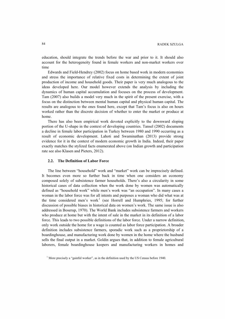
cross-sectional relationship. The basic difference between the two sets of results is that in the average OLS the point estimates imply a trough in the U-shape later in the development process than in the panel regressions (our values from the panel regressions are comparable to the estimates in Tam’s paper). The results from Table 1a imply a trough at between 6000$ and 7700$ (2005 dollars). Figure 1 presents a scatter plot of female participation against log income, having subtracted the effect on the intercept of the cultural variables, based on estimates in column 4 of Table 1a. The U-shape is visually evident.

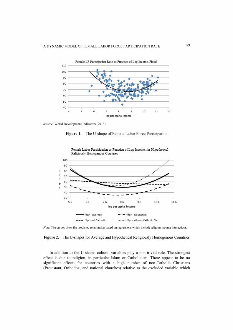
In column 5 we allow the sensitivity of labor force participation to vary with religious affiliation, estimating a “religion-adjusted” U-shaped curve. For sake of completeness we have also ran the regressions with interactions between the colonial and geographic variables (not reported). While, to economize on space, we don’t present the numerical values of the estimates, in Figure 2 we show the implied U relationship for the “average” country as well as for hypothetical religiously homogenous countries.


89

Source: World Development Indicators (2013)

Figure 1. The U-shape of Female Labor Force Participation

Note: The curves show the predicted relationship based on regressions which include religion-income interactions.

Figure 2. The U-shapes for Average and Hypothetical Religiously Homogenous Countries

In addition to the U-shape, cultural variables play a non-trivial role. The strongest effect is due to religion, in particular Islam or Catholicism. There appear to be no significant effects for countries with a high number of non-Catholic Christians (Protestant, Orthodox, and national churches) relative to the excluded variable which

RADEK SZULGA 90

includes Buddhism, Hinduism, Judaism, several smaller religions as well individuals who claim no religion. To control for other possible cultural factors we also include controls for former colonial status (including former Soviet and former Soviet block countries) and geographic location. For example, the effect of secularism might be due to the fact that a number of these countries are either former republics of the Soviet Union, or former Soviet satellite states. Likewise, it’s quite possible that a significant difference exists among majority Catholic countries which were colonized by Spain, by France, or never colonized. Muslim majority countries in the Middle East might be quite different from Muslim countries in South East Asia.

These hypotheses are mostly affirmed. Former Soviet republics do have higher female labor force participation even once the degree of secularism is controlled for, and this is true even for former Soviet republics with a high percentage of Muslims such as Tajikistan and Uzbekistan. Countries which are former Spanish or Portuguese colonies have lower female labor force participation rates, and the inclusion of these variables lowers the estimated effect of Catholicism. At the same time the control for being a former French colony has a positive sign (only significant in the OLS specification), suggesting that overall for developing countries it might be Iberian-derived Catholic culture which lowers female labor force participation more than Francophone Catholic culture.3 Somewhat mysteriously, countries which were colonized by other European states (former colonies of Germany, Belgium and Netherlands) have higher female labor force participation, although that effect could be driven by a few outliers (in particular, Indonesia). Finally, the results also show that countries in the Middle East and North Africa have substantially lower female labor force participation rates even controlling for the effect of Islam. This effect is also noted in Rauch and Kostyshak (2009).

Table 2 presents the results of regressions which utilize latest Barro and Lee (2012) data on educational attainment and economic development. The dependent variable is the ratio of average years of total schooling for females relative to males. Unsurprisingly this ratio increases with per capita income. Visualization of the data as in Figure 3 suggests that the relationship is non-linear since above a certain level the ratio reaches an upper bound and further increases in income play a muted role. Consequently we also estimate a structural break model. We do a grid search over possible threshold levels of income which yield the best fit to the data (by minimizing the sum of squared residuals), where both the slope and the intercept are allowed to change. Somewhat reassuringly we find that both the intercept and slope have the largest statistical change at the same log income of 8.7, which corresponds to per capita income of about 6000$ (in 2005 dollars). At income levels lower than that, a 10% increase in per capita income increases the female-male education ratio by about 0.011, while above this threshold the increase is much smaller, at about 0.049. Once again we employ both pooled OLS and panel

3 Allowing for additional interaction between the “Former Iberian” and “Former French” dummies and

income indicates that there is quite a bit of a different pattern for these two sets of highly Catholic countries.


91

estimation, although in our panel regressions no structural break shows up as significant.

Table 2. Female-Male Education Ratio Dep. Variable: Ed ratio OLS OLS PANEL, FE PANEL OLS, THR

Log income 0.102*** 0.0939*** 0.0964*** 0.0912*** 0.114*** (0.00391) (0.00685) (0.0113) (0.0144) (0.0175) % Muslim -0.0797*** -0.0879* (0.0227) (0.0504) % Catholic 0.00945 -0.00320 (0.0228) (0.0529) % Non Cath. Ch. 0.0364 0.0221 (0.0223) (0.0493) F. British 0.0445*** 0.0397 (0.0129) (0.0293) F. Iberian 0.0262 0.0175 (0.0238) (0.0587) F. Soviet 0.0882*** 0.103* (0.0285) (0.0579) F. Soviet block -0.0221 -0.00358 (0.0250) (0.0505) F. French -0.0535*** -0.0659* (0.0160) (0.0363) F. Other Eu 0.140*** 0.134*** (0.0238) (0.0409) Income threshold 8.7 0.642*** (0.137) Interaction threshold 8.7 -0.0656*** (0.0186) Regional dummies No Yes No Yes No Constant -0.0426 -0.0443 0.00576 -0.00686 -0.172 (0.0368) (0.0564) (0.103) (0.120) (0.123) Observations 885 883 885 883 885 R-squared 0.436 0.641 0.494 Number of index 138 137 Notes: Robust standard errors in parentheses. *** p<0.01, ** p<0.05, * p<0.1. Dependent variable is average years of total education for females relative to males. Sources: Education data are from Barro and Lee (2013). Income data is from World Development Indicators (2013). Religious data is from the CIA Factbook (2013).

RADEK SZULGA 92

Figure 3. Female-Male Education and per Capita Income

4. THE MODEL In this section we present the model which accounts for the stylized facts and

empirical results highlighted above. There are two goods, two factors, and two production sites. The two goods are a “market” good (food or income) and a “household” good (child rearing). For simplicity, utility is linear. The two production sites are a “traditional” production site (the farm) and a “modern” production site (the city). Each household makes a location decision as to where its economic activities will be undertaken. The trade off involved is that while the market wage may be higher in the city, there are economies of scope on the farm, which allow female labor to be supplied simultaneously to household and market production. The intuitive example is that of much of agricultural work, or traditional cottage production, which can be carried out while the children are present. This in turn means that the children can be reared at the same time as work for income is being done. This generally is not an option for factory or office work.

The two factors are male and female labor. Male labor can only be used in market production. Female labor can be used to produce either good. Perhaps ironically, it is precisely the fact that female labor is more productive in both the household and (weakly) in the market sector that results in the gender specific specialization and the consequent lower accumulation of female human capital. The choice is made on the basis of comparative, not absolute, advantage. Since utility is linear, if the household is located in the city, female labor will only be supplied to the one sector where its productivity is higher. Hence the labor supply choice for the households in the city is a binary one; whether women will work in the house or in the market.


93

4.1. Static Location Decision The production function for market work on the farm is given by FFF LAY = where

FA is productivity and FL is labor employed in the market good sector on the farm. We assume perfect competition in the labor and goods market so labor gets its marginal product and the wage rate on the farm is just FF Aw = (implicitly we are normalizing the price of the market good to 1). Analogously we have CCC LAY = and CC Aw = in the city, with FC AA > .

Households are differentiated by their endowments of human capital. For simplicity (this can be easily relaxed) we assume that the initial endowment of male human capital is the same as that of female human capital within each household. We denote these endowments as Mh and Fh . Once we introduce investment in human capital into the model, each h will change over time and female and male human capital levels will diverge. The role of human capital is that it determines the effective labor endowment of each household that can be supplied to the market sector. Each household is endowed with 1 unit of male and 1 unit of female labor and h is a quality adjustment. Hence a household has FM hh + units of effective labor to supply.

The production side of the model is similar to the standard AK or related endogenous growth models, with human capital instead of physical capital. Technological growth then can be thought of as embodied in human capital accumulation. A change in the productivity parameter, CA , will have an effect that is analogous to an increase in the marginal product of capital in the AK model; the growth rate of per capita income will increase. The precise effect of such a shock on labor force participation and human capital investments is discussed in Section 5 which analyzes the wage elasticity of labor force participation.

Finally we assume that production of the household good does not depend on female human capital, although we do assume that human capital is transferred inter- generationally. Since utility is linear, either 0 or 1 unit of female labor will be used in household production. The utility value of the household good produced is denoted by P. One period utility, without the cost of investment is then:

⎢⎢⎢

⎣

⎡

=+

=+

=+

=

3)(

2

12

),(

sifAhh

sifPAh

sifPA

tsm

CFM

CM

F

. (1)

A farm household is denoted by 1=s , a single earner city household is 2=s , and

a two earner city household is 3=s . We assume the cost of investment is quadratic. The net per period utility is then

RADEK SZULGA 94

22 )(2

)(2

),(),( tiφtiφtsmtsu FM −−= , (2)

where Fi is investment in female education, Mi investment in male education, and φ is a scale parameter affecting the marginal cost of investment. s is a choice variable (and a function of time), albeit a discrete one. The cost of investing in human capital is independent of the state the household is in. The household will choose the state which maximizes its current utility, and choose the levels of investment to maximize its remaining lifetime utility. We can find the loci of points which indicate combinations of male and female human capital at which a household will be indifferent among its various location/labor supply options. These three boundary lines are illustrated below in Figure 4, where the numbers indicate the optimal s for the relevant region.

.2

,

,2

3113

3223

2112

mmhA

PAh

mmAPh

mmAAh

M

C

FF

C

F

C

FM

=⇔−+

=

=⇔=

=⇔=

(3)

Figure 4. Indifference Loci in Mh , Fh Space: The Household Starts Off in Area 1


95

In the figure above Area 1 corresponds to the values of Mh and Fh when state 1 is optimal and so forth. Initially the different households are located in the FM hh / space along a ray from origin. Hence the set of households in each area is given by

.2),(

,2),(

,22),(

3

2

1

⎭⎬⎫

⎩⎨⎧

−+

>>=

⎭⎬⎫

⎩⎨⎧

<>=

⎭⎬⎫

⎩⎨⎧ +

<<=

Mj

C

FFj

C

Fj

Mj

Mj

C

Fj

C

FMj

Mj

Mj

C

FFj

C

FMj

Mj

Mj

hA

PAhandAPhhhS

APhand

AAhhhS

APAhand

AAhhhS

(4)

In the following sections we analyze what happens to the households as their

position changes through time due to investment in human capital and how the relative size of the above sets changes.

4.2. Investment Decision and Dynamics of a Single Household We assume that each household starts with initial levels of Mh and Fh low

enough such that state 1 is initially optimal, C

FM

AAh 2)0( < and

C

M

APh <)0( and

PAF <2 , i.e., farm productivity is substantially lower than household productivity, which is plausible for economies at very low level of development. This assumption is also crucial for the model to generate the U-shaped female labor force participation rate found in the data since otherwise at least some households would go straight from Area 1 (farm, both work) to Area 3 (city, both work). Lifetime utility is:

dtetuU tβ

s∫∞ −=0

)( . (5a)

The laws of motion for human capital are: )(tih M

t

M=

∂∂ and )(tih F

t

F=

∂∂ . This

simple formulation embodies two important assumptions. First, human capital is transferred inter-generationally, so that even in the absence of investment, children will have a positive level of human capital inherited from their parents. One way to understand this assumption is to think of human capital as being produced, with parents’ human capital and investment as two separate but substitutable factors of production. Several papers provide empirical support for such an influence, whether through the effect of parents’ education on children’s health outcomes, social skills. or basic literacy and numeracy (Chen and Li, 2009; Currie and Moretti, 2008; Moore and Schmidt,

RADEK SZULGA 96

2004). Second, we are also assuming that the inter-generational transfer of human capital

takes place along gender lines; daughters inherit human capital from mothers, sons from fathers. This assumption is obviously stronger and potentially unrealistic. A more general version of the model would allow for human capital to be inherited from both parents. In that case the model becomes much more complicated and difficult to solve and much of the intuition gets lost in the algebra. At the same time the basic qualitative results - the existence of the U-shape and other stylized facts - are not affected, although the speed of dynamics and the precise timing of switching between Areas may be different.4

The dynamic optimization problem of the household then is:5

∫∞ −= 0,, ),( tβ

siis etsuUMax MF . (5b)

There are three possible steady states, in terms of the choice of both )(ti s and )(ts

corresponding to three possible dynamic paths: i) Never invest, stay on farm the forever. ii) Invest only in male education, initially stay on the farm and then when Mh is

high enough move to the city and stay a one-earner household forever. iii) Invest in both male and female education while on the farm, move northwest

until FM hth 12)( = then switch to a single earner city household, keep moving northwest

and switch to a two-earner city household when FF hth 23)( = , then keep investing in both forever.6

For plausible parameter values possibilities 1 and 2 are dominated by possibility 3. Hence we concentrate on solving the problem involving this particular steady state. In this case we can write the lifetime utility as a sum of four parts - utility while in state 1, utility in state 2, utility in state 3, and subtract the present value cost of investing in both

4 If human capital is inherited as a weighted average of both parents’ human capital, the model constitutes

a system of two interdependent non-homogenous differential equations rather than two separate equations which can be solved individually. The basic difference is that the “averaging out” of human capitals in that case tends to pull the path in Figure 5 towards the 45 degree line. However, as long as payoffs to male human capital commence before payoffs to female human capital, the overall qualitative result is the same.

5 Note also this dynamic optimization problem can be solved in the usual manner with Hamiltonians, though here we wish to focus on the intuition behind the result.

6 State 1 - stay on the farm forever - would be optimal if the “modern sector” productivity is very low relative to both farm and household productivity. State 2 could be optimal if household productivity is high relative to “modern sector” productivity. This means that it is possible for economies to get stuck in poverty traps in this model, although the reasons for such an outcome are beyond the scope of this analysis.


97

types of human capital:

.22

)()()2(

00

0

22

2

2

1

1

tβMtβF

tβt C

FC

Mtβtt C

Mt tβF

eiφeiφ

eAhAhePAhdtePAU

−∞∞ −

−∞−−

∫∫

∫∫∫

−−

+++++= (6)

Here 1t and 2t are the times at which the household switches from state 1 to state

2 and from state 2 to state 3, respectively. These are determined by the values of Mh and Fh . Hence the optimal switching time is implied by particular paths of )(tiM and

)(tiF . Consider a household which has invested enough in Mh and Fh in the past so that it is about to enter area 3. Since this is a steady state it plans on staying here forever. In this case the marginal benefit of a unit of investment in either type of human capital is

βAC , while the marginal cost is just the amount of investment, times φ . Hence

investment is φβAC for both female and male education for 2tt > . Now consider the

choice of investment before the household enters Area 3. Before entering Area 3, the household will choose 2=s . At this point it will receive the benefit from having the

male work in the market, hence the optimal value of )(tiM here is still φβAC .

While in state 2, the household receives no present utility from female human capital. It anticipates that in the future, once Fh is high enough, the female member of the household will work, and hence it pays to invest in female education right now. This benefit has to be discounted by the time it will take the household to move from its current position inside Area 2 to the boundary between Areas 2 and 3. The marginal

benefit of investment in female education at this stage is given by )( 2 ttβC eφβA −− which

will be the level of investment in female education for 2tt ≤ . Note that the same reasoning applies to investment in female education while in Area 1. Similarly, while in Area 1 investment in men’s education has to be discounted by )( 1 ttβe −− . The paths for investment then are:

⎢⎢⎢⎢

⎣

⎡

≥

≤=

−−

KC

KttβC

K

ttifφβA

ttifeφβA

ti

K )(

)( , (7)

RADEK SZULGA 98

where K denotes either male or female investment and }2,1{∈k . The ratio of female to male investment in human capital is implicitly illustrated Figure 5.

Figure 5. The Dynamic Path of Female and Male Human Capital

This is also the slope of the dynamic path in FM hk / space. The slope of this path

is positive and concave, and it approaches 1 as the household enters Area 3. This aspect of the model is just stylized fact 3. Over the course of development male education begins to rise first and only later does female education begin catching up with it. Knowing the level of investment at each time allows us to rewrite utility in terms of parameters and maximize it with respect to 1t and 2t . Alternatively, we know that 1t will occur when the household moves from its initial position to the point at which it wants to switch to state 2:

speedaverageboundarytocetandist =1

∫

−=

1

01

1

)0(2

t M

M

C

F

it

hAA

,

which means )0(2)1( 12

M

C

FtβC hAAe

φβA

−=− − . Solving this equation for optimal time to

switch from state 1 to state 2 we have


99

⎥⎥⎦

⎤

⎢⎢⎣

⎡⎟⎟⎠

⎞⎜⎜⎝

⎛−−−= )0(21ln1 2

1M

C

F

Ch

AA

Aφβ

βt , (8)

which can also be obtained from maximizing lifetime utility with respect to 1t . Here we can see the necessary condition for path 3 to dominate paths 1 and 2; 01 >t . 2t is derived in a similar manner. In both cases )0(h needs to be less than the indifference value but not so small (alternatively FA and P big enough) that the above expressions become undefined.7 These are also the conditions needed to ensure that Possible Path 3 dominates the other two.

The above investment levels imply

⎢⎢⎢⎢

⎣

⎡

≥−+

≤−+

=

−

KkC

C

KtβtβCK

K

ttifttφβA

Av

ttifeeφβAh

th

K

)(

)1()0()(

2

, (9)

where K and k are as before, and },2{ PAυ F∈ . The present discounted value of lifetime utility as a function of 1t and 2t is

( ).)2()2(21

)0()0()1()1(2

2211

2121

2

2tβtβtβtβC

tβFC

tβMC

tβtβF

eeeeφβA

ehAehAePeAUβ

−−−−

−−−−

−+−+

++−+−= (10)

The first term is the value of market wages from agriculture for both members of the

household until 1t . The second term is the value of household production until 2t , when the female ceases to work at home, the third and fourth terms are the values of initial human capital for male and female appropriately discounted from the time when they first become utilitized and the last term is the net value of investment for both members of the household. Maximizing the above utility function with respect to 1t and 2t yields the values for 1t and 2t given above. Figure 6 shows the paths of total cost of investment, household production, market income and net utility for the values

}22,22,12,8,5.0{ ===== φPAAβ CF .

7 Formally we need that 2

2)0(2φβA

AAh

AA C

C

FM

C

F −>> and 2

)0(φβ

AAPh

AP C

C

F

C−>> .

RADEK SZULGA 100

Figure 6. Evolution of Key Variables; Including Total Investment in Human Capital,

Household Production, Market Income and per Period Utility of Households 4.3. Distribution of Households and Labor Force Participation Over Time Next we consider how the distribution of households changes over time. We let j

index both households and their initial position, so that jjhjh MF == ),0(),0( and with only a slight loss of generality we assume }1,0{∈j , normalizing the measure of households to 1. For example, 9.0=j is the “90th percentile” household. It is straightforward to generalize the model to allow for population growth, in which case the distribution of households may “stretch” over time. Such changes can have important implications for the distribution of income and the precise results depend on how newly born individuals are matched up. However, the consideration of these effects is beyond the scope of this paper.

We denote by )(1 tj the household, if any, which at time t finds itself on the

boundary C

FM

AAh 2

12 = . Similarly we make )(2 tj be the household, if any, which at

time t finds itself on the boundary C

F

APh =23 . As households begin their journey across

the FM hh / space there are two possibilities for how they become allocated.


101

First we have the case where there are never households in all three areas simultaneously. This occurs if the lowest household ( 0=j ) which enters Area 2 does so before the highest household ( 1=j ) crosses into Area 3. Alternatively it could be the case that the highest ability household starts entering Area 3 while there are still some households in Area 1. We analyze the former case first and normalize time so that at

0=t the highest ability household is located right on the boundary C

FM

AAh 2

12 = . In the

next instant of time additional households begin entering Area 2. The proportion of households in Area 1 is )(1 tj and those in Area 2, ( )(1 1 tj− ), up until 0)(1 =tj . Given 0>t we want to find the household on the boundary, if any, such that

)1(2 )(2112

11 −+== − tβjtβC

C

FM eeφβAj

AAh . Solving this for )(1 tj we have

⎢⎢⎢

⎣

⎡ ∈−−=

−

otherwise

tttifeφβA

AA

tjtβC

C

F

0

],[)1(2)(

11

012

1 , (11a)

where 0

1t and 11t are the times when the lowest and highest initial ability household

each cross the first boundary, C

FM

AAh 2

12 = , respectively. The number of households on

the farm is falling at a decreasing rate, while the number in the city with only the male working in the market is increasing at a decreasing rate. Eventually all households pass into Area 2 and at some future time begin entering Area 3. At that point the proportion of households in Area 2 is )(2 tj , and that of those in Area 3 by )(1 2 tj− .

⎢⎢⎢

⎣

⎡ ∈−−=

−

otherwise

tttifeφβA

AP

tjtβC

C

0

],[)1()(

12

022

2 , (11b)

where 02t and 1

2t are defined analogously with respect to the boundary C

F

APh =23 .

Putting all this together we get the paths for the share of the households in each area shown in Figure 5 below. The female labor force participation rate is just the inverse of the share of households in Area 2. The analysis for the case where there is an overlap between households which are entering Area 2/leaving Area 1 and those entering Area 3/leaving Area 2 is similar.

RADEK SZULGA 102

5. SIMULATION AND STYLIZED FACTS In this section we present results which illustrate how the model replicates the

stylized facts presented in the introduction. Note that the proper interpretation of model time is a generation. The motivation for investment in human capital while on the farm is the anticipation that someday one’s children or grandchildren will leave the farm and work in the city. This assumes a production function for children where human capital is passed down from parent to child according to sex (the implications of this assumption are discussed above), as well as the absence of structural impediments to the development process which could get the economy permanently stuck in the traditional.

5.1. Stylized Fact 1 The female labor force participation rate, is U-shaped. This immediately follows from the signs of the first and second derivatives:

021 <−=∂∂

=∂∂ − tβC e

φβA

tj

tj and 02

22

21

2>=

∂∂

=∂∂ − tβC e

φA

tj

tj ,

and the fact that female labor force participation is given by:

⎢⎢⎢⎢⎢⎢⎢

⎣

⎡

>

≤≤−

≤≤−+

≤≤

≤

=

02

02

012

01

1221

12

111

11

1

)(1

)()(1

)(

1

)(

ttif

tttiftj

tttiftjtj

tttiftj

ttif

tflfpr , (12)

in the case where parameters are such that 0

112 tt < (similar results hold if 0

112 tt > ).

The two possible path for female labor force participation rate is illustrated Figure 7. In both cases the path of female labor force participation is U-shaped. In the

remainder of this section we focus on the first case.


103

Figure 7. U-shaped Female Labor Force Participation in Two Cases, Depending on How Dispersed the Households Are Initially

5.2. Stylized Fact 2 At the beginning of the development process the average education of women in

labor force is lower than that of women in general, but this reverses itself over time. Goldin (1992, p. 135) points out that although presently women in the labor force

have higher levels of education than women on average, this has not been true historically. In the first decade of the twentieth century the average years of schooling of a woman in the labor force was less than seven years, while that of an average woman in the population was eight years. A lot of women who were not in the labor force had higher levels of education than working women. For a number of developing countries the same phenomenon can be observed presently as suggested by the regressions above. By the time of World War II the US average working woman had an extra year over the average woman. Hence there was a significant change in the educational composition of the female labor force vis a vis the female population in general. The model replicates this fact. If we believe that for the US the trough of the U-shape occurred sometime

RADEK SZULGA 104

around the turn of twentieth century then it is precisely at this time that the education of labor force participants would begin to catch up with that of women in general, as high ability households began turning into two worker families. A similar pattern has also been documented in the specific micro level context of the state of Rhode Island in the 1960’s in Mott (1972).

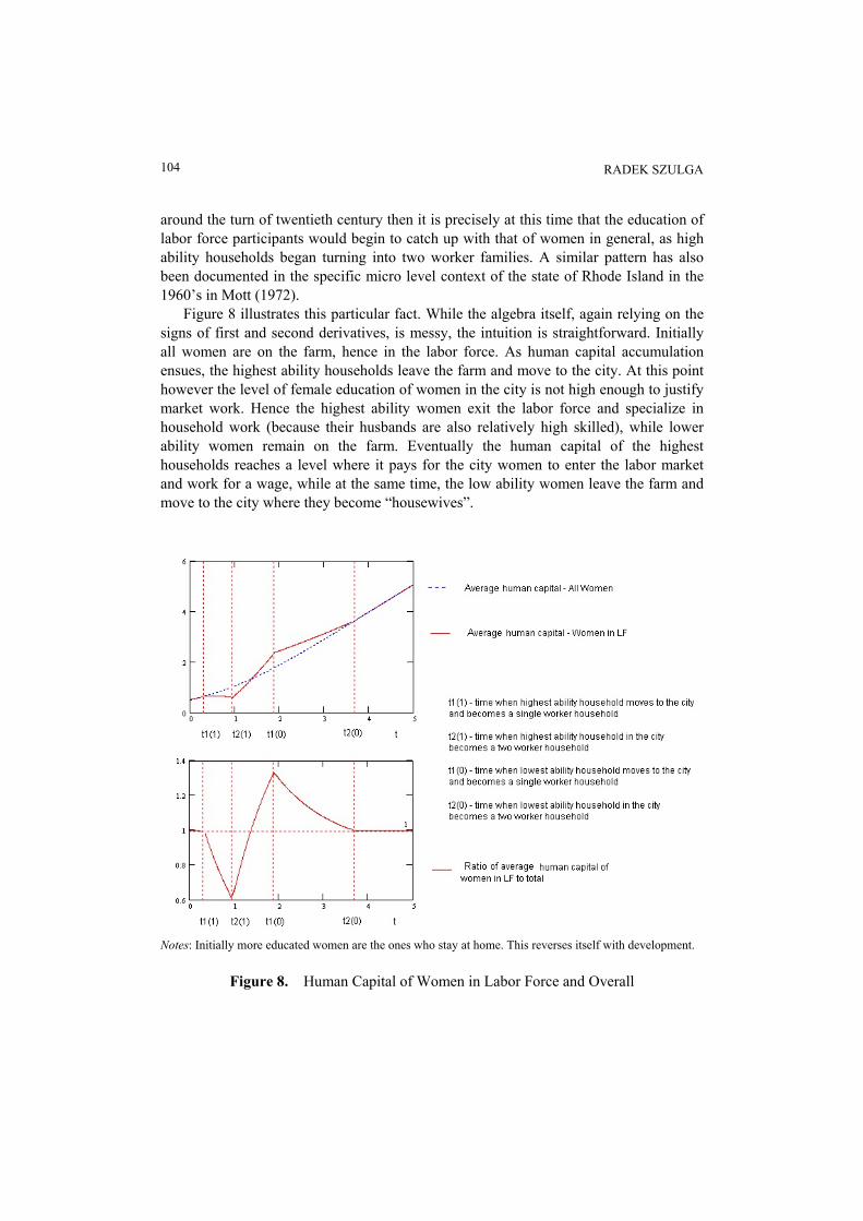
Figure 8 illustrates this particular fact. While the algebra itself, again relying on the signs of first and second derivatives, is messy, the intuition is straightforward. Initially all women are on the farm, hence in the labor force. As human capital accumulation ensues, the highest ability households leave the farm and move to the city. At this point however the level of female education of women in the city is not high enough to justify market work. Hence the highest ability women exit the labor force and specialize in household work (because their husbands are also relatively high skilled), while lower ability women remain on the farm. Eventually the human capital of the highest households reaches a level where it pays for the city women to enter the labor market and work for a wage, while at the same time, the low ability women leave the farm and move to the city where they become “housewives”.

Notes: Initially more educated women are the ones who stay at home. This reverses itself with development.

Figure 8. Human Capital of Women in Labor Force and Overall


105

5.3. Stylized Fact 3 Initially men’s education rises faster than women’s. Hence the ratio of male to

female education falls. Eventually this reverses itself and the ratio approaches one as time goes to infinity.

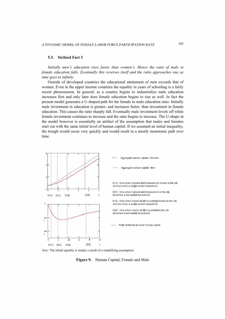
Outside of developed countries the educational attainment of men exceeds that of women. Even in the upper income countries the equality in years of schooling is a fairly recent phenomenon. In general, as a country begins to industrialize male education increases first and only later does female education begins to rise as well. In fact the present model generates a U-shaped path for the female to male education ratio. Initially male investment in education is greater, and increases faster, than investment in female education. This causes the ratio sharply fall. Eventually male investment levels off while female investment continues to increase and the ratio begins to increase. The U-shape in the model however is essentially an artifact of the assumption that males and females start out with the same initial level of human capital. If we assumed an initial inequality, the trough would occur very quickly and would result in a mostly monotonic path over time.

Note: The initial equality is simply a result of a simplifying assumption.

Figure 9. Human Capital, Female and Male

RADEK SZULGA 106

The value of the minimum depends negatively on P and positively on both city and farm wages. These effects are intuitive. A higher productivity in the household means that a higher level of female education is needed to justify market work for women. Hence households will spend a longer time on the farm and in the city as single worker families. This in turn slows down investment in female education without affecting investment in male education, hence resulting in a larger gap between the educations of the two groups.

A higher market wage in the city works similarly except that it speeds up the

investment of both men and women. However, since the boundary CA

P changes more

than the boundary C

F

AA2 , less time will be spent by each household in Area 2. This

implies that the increase in female education investment due to a higher market wage will be greater than the increase in male education investment, resulting in a smaller gap.

An increase in the farm wage has the effect of delaying the shift from farm to the city. As long as the increase in FA is not too big (so that FAP 2> continues to hold) this will lower investment in male education for farm households, while leaving female education investment unchanged (since this depends only on CA and P). Therefore, the human capital gap between the two members of the households will be less pronounced.

5.4. Stylized Facts 4 and 5: Income and Wage Effects The consideration of income and substitution effects on women’s labor force

participation, particularly for married women, goes back to at least Mincer (1962). Historically for the United States the effect of a change in husband’s income on the female labor force participation rate has not remained constant (Goldin, 1992, p.133). At the turn of the century the income effect was negative and substantial (an increase in men’s income tended very strongly to push women out of the labor force), while the wage effect was positive, albeit small. As Goldin puts it “A married women was not easily enticed into the labor force by higher wages, but she was, at the same time, encouraged to leave by higher earnings of her husband and other family members.” By the time of World War Two the income effect had declined in size while the wage effect increased. Presently both wage and income effects are small in magnitude. Once again, we illustrate below that the model replicates these facts.

To analyze the effects of income and wage increases on female labor force participation rate in the model we distinguish between male and female wages in the city although so far we have assumed that these are equal. Hence the relevant boundaries become M

CF wA /2 and FCwP / , where M

Cw is the male wage in the city and FCw is

the analogous female wage. We identify income effects with the change in female labor force participation due to a change in M

Cw , MCwflfpr Δ/Δ , and wage effects with the


107

change in female labor force participation due to a change in FCw , F

Cwflfpr /Δ . Note that in contrast to most of previous work we are not dealing with changes in hours of labor supplied per women, but rather the change in the number of women working.

When considering shocks to wages we need to distinguish between anticipated and unanticipated shocks. Unanticipated shocks have the effect of only changing a given household’s optimal location, whereas anticipated shocks will also affect the entire path of investment and human capital. Below we focus on unanticipated shocks.

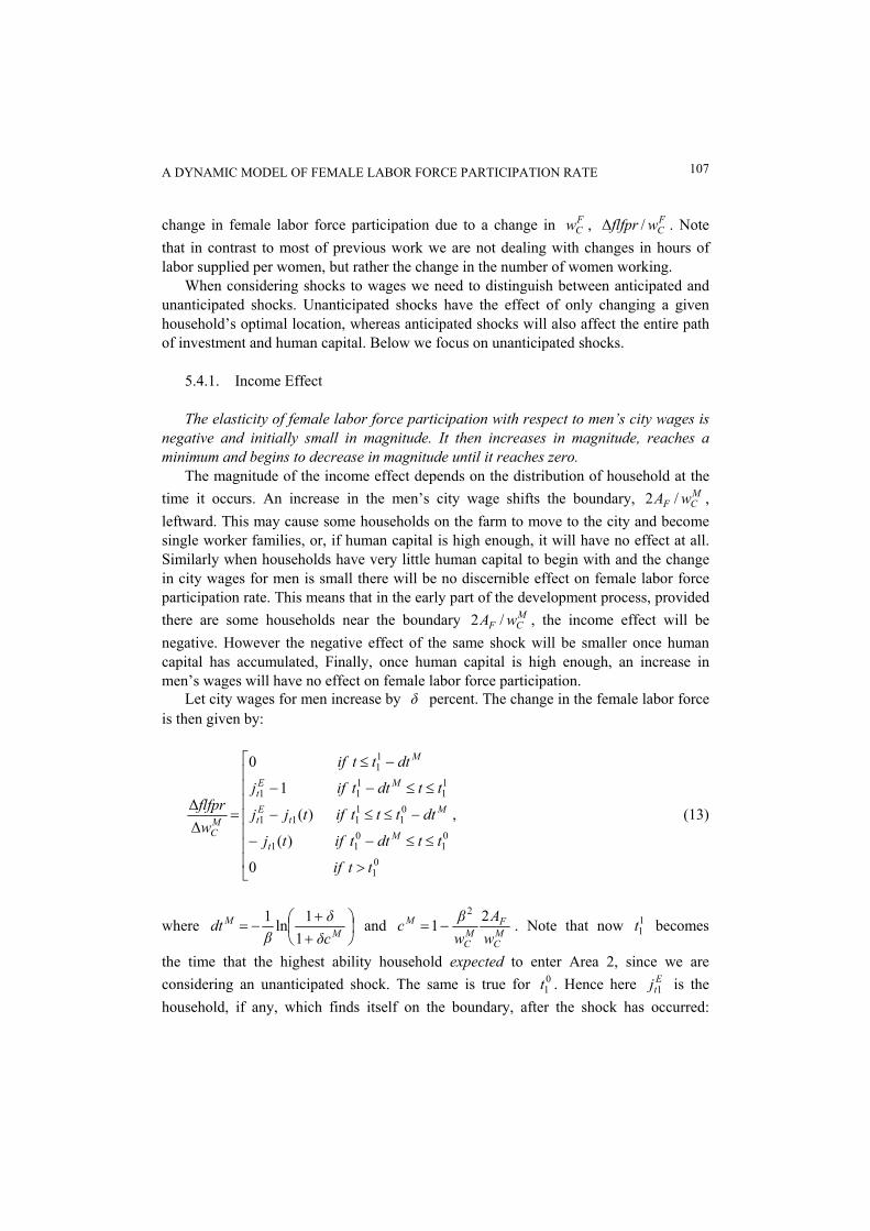
5.4.1. Income Effect The elasticity of female labor force participation with respect to men’s city wages is

negative and initially small in magnitude. It then increases in magnitude, reaches a minimum and begins to decrease in magnitude until it reaches zero.

The magnitude of the income effect depends on the distribution of household at the time it occurs. An increase in the men’s city wage shifts the boundary, M

CF wA /2 , leftward. This may cause some households on the farm to move to the city and become single worker families, or, if human capital is high enough, it will have no effect at all. Similarly when households have very little human capital to begin with and the change in city wages for men is small there will be no discernible effect on female labor force participation rate. This means that in the early part of the development process, provided there are some households near the boundary M

CF wA /2 , the income effect will be negative. However the negative effect of the same shock will be smaller once human capital has accumulated, Finally, once human capital is high enough, an increase in men’s wages will have no effect on female labor force participation.

Let city wages for men increase by δ percent. The change in the female labor force is then given by:

⎢⎢⎢⎢⎢⎢⎢

⎣

⎡

>

≤≤−−

−≤≤−

≤≤−−

−≤

=

01

01

011

01

1111

11

111

11

0

)(

)(

1

0

ΔΔ

ttif

ttdttiftj

dttttiftjj

ttdttifj

dtttif

wflfpr

Mt

Mt

Et

MEt

M

MC

, (13)

where ⎟⎠⎞

⎜⎝⎛

++

−= MM

cδδ

βdt

11ln1 and M

C

FMC

M

wA

wβc 21

2−= . Note that now 1

1t becomes

the time that the highest ability household expected to enter Area 2, since we are considering an unanticipated shock. The same is true for 0

1t . Hence here Etj 1 is the

household, if any, which finds itself on the boundary, after the shock has occurred:

RADEK SZULGA 108

)1()1(

221

tβMMCtβ

MC

FEt ec

βwe

wδAj −− −+

+= .

As a result the income effect is small at the beginning and end of the development process and large in the middle. Goldin finds that in the first two decades of the twentieth century the income effect appeared to be large in magnitude but has since moved closer to zero, especially in the post World War Two era. At the same time the trough of the U-shape likely occurred during the same time. The turn of the century then represents the middle of the development for countries such as the US. The model is consistent with the empirical finding of a large negative income effect at the turn of the century, which subsequently diminished. Furthermore it provides an explanation for the fact that the change in male wages in the industrial sector is likely to have a large effect if there are a large number of households who are close to being indifferent between the traditional sector and moving to the city. The resulting rural-urban migration induces households to become single worker families in the city as married women specialize in household work and child rearing.

The figures below illustrate the level change and the elasticity of female labor force participation with respect to male city wages. The parameters are the same as above and the shock is an unanticipated increase of 10% in city wages.

Figure 10. The Income Effect, Change and Elasticity.


109

The figure illustrates both absolute changes and the elasticity. In the second panel, for the parameters chosen, at its most extreme, a 10% change in men’s city wages decreases female labor force participation by roughly 25%. This is the case where the change in wages sweeps almost all households remaining on the farm into the cities, pushing female market attachment down to zero.

5.4.2. Wage Effect The elasticity of female labor force participation with respect to women’s city wages

is positive and initially small in magnitude. It then increases, levels off, and becomes zero once all households have moved to the city.

The wage effect works in an opposite, but similar way to the income effect. When households have very low human capital a discrete change in female wages will have no effect on the location decision of households and hence no effect on female labor force participation rate. As households move northwest in the MF hh / space a female wage

shock, which shifts the FCwP boundary downward, will cause some single worker

households in the city to begin supplying female labor to the market. This effect initially increases as more households approach the boundary, and then begins to decrease. In percentage terms, the own-wage elasticity of female labor force participation is initially small and increases over the course of development. At its peak, which roughly occurs sometime after the trough in the female labor market attachment is attained, a 10% increase in female city wages results in about a 25% increase in female labor force. The wage effect is given by:

⎢⎢⎢⎢⎢⎢⎢

⎣

⎡

>

≤≤−

−≤≤−

≤≤−−

−≤

=

02

02

022

02

1222

12

122

11

0

)(

)(

1

0

ΔΔ

ttif

ttdttiftj

dttttifjtj

ttdttifj

dtttif

wflfpr

Ft

FEtt

FEt

F

FC

, (14)

where 1

2t and 02t are defined similar to above except with respect to the expectations

regarding the FCwP boundary. Furthermore E

tj2 is given by

)1()1( 22

tβFFCtβ

FC

Et ec

βwe

wδPj −− −+

+= ,

RADEK SZULGA 110

where now ⎟⎠⎞

⎜⎝⎛

++

−= FF

cδδ

βdt

11ln1 and F

C

CFC

F

wA

wβc 21

2−= .

Figure 11 illustrates the effect of a shock to female wages on female force participation rate as a function of time (that is, as a function of the distribution of households at a particular moment in time).

Figure 11. The Wage Effect, Change and Elasticity

6. SOME POLICY IMPLICATIONS The model of this paper has two important implications for both theoretical and

empirical work on economic growth and how it relates to female education and labor force participation. Some of the older literature in growth empirics had uncovered a bit of a puzzle. In many specifications female education is negatively correlated with subsequent economic growth. In the popular textbook of Barro and Sala-i-Martin, (1995)


111

this appears as a frequent and robust result.8 The authors attribute it to the fact that a low female to male education ratio is a proxy for low level of development and hence is picking up convergence effects. However, this paper suggests that this negative correlation may arise from the interaction of female labor force participation and education. Although in our model female education and market income increase concurrently, for the middle stage of the development process, the rise in market income is solely due to the increases in male education. Hence, the empirical result could simply be due to the fact that in developing countries many educated women never enter the labor force. Rather, female education represents investment in intergenerational human capital transfer, as the acquired skills are passed down to the children. This implies that even if existing data show no (or even negative) relationship between female education and growth that does not imply that the return to female education is unimportant. The benefits are simply further off in time, when the children enter the labor force. Even long panel estimates of ten year periods, may not be able to pick up these effects.

Second, in our analysis we have ignored the two possible steady states which correspond to a “poverty trap” and even a “middle income trap”; the “don’t invest, stay on farm forever” and the “invest only in male education, remain a single earner household forever” paths. Impediments to investment in female education and/or low returns to women’s labor in the market are exactly the conditions under which the economy is more likely to get stuck in these undesirable situations. Together these factors (high φ , low CA for women) can be taken as representative of institutional barriers to both female education and economic development (for a broad discussion of such factors see King and Hill, 1997). While here the causality would run from these “bad institutions” to lack of growth and education, at the very least the fact that a particular economy is not investing in women’s education serves as a clear signal that the country is stuck in a poverty trap. More generally, the model suggests that getting out of such a trap requires a reduction in these obstacles as well as an effort to promote women’s education - Target 3A in the Millennium Development Goals (UN, 2012). In fact, even in absence of other reform, increasing female education could move a household from Areas 1 or 2 to Area 3 and result in further self sustaining investment in human capital.

7. CONCLUSION In this paper we develop a dynamic model of female participation rate and education

which broadly matches several stylized facts found in the data. For empirical inspiration and support we have mostly relied on Claudia Goldin’s “Understanding the Gender

8 Lorgelly and Owens (1999) and Lorgelly et al. (2001) have questioned this finding as arising from presence of outliers or some form of model misspecification.

RADEK SZULGA 112

Gap” and the literature on female labor force participation both in developing countries and historically in developed countries. We provide both an intuitive justification for the processes for dynamic phenomenon which are summarized in the five stylized facts listed in the introduction, as well as a formal analysis. The underlying assumption is that of economies of scope in the traditional sector and the resulting tradeoff between locating one’s productive activities “on the farm” or “in the city” and choosing between operating as a single earner or two earner household.

The model can be readily extended in several ways. For one, we can explicitly incorporate unmarried women in to the model and see if the resulting dynamics produce the married/unmarried substitution evident in history (intuition and some preliminary work seem to indicate that this is indeed the case). More substantially, the model could be expanded to include an explicit fertility choice and a production function for children’s human capital. In this case an over lapping generations framework might be better suited rather than the continuous time model presented here.

REFERENCES

Adams, J. (1988), “Decoupling the Farm and the Household: Differential Consequence of Capitalist Development on Southern Illinois and Third World Family Farms,” Comparative Studies in Society and History, 30(3), 453-482.

Arellano, M., and S. Bond (1991), “Some Tests of Specification for Panel Data: Monte Carlo Evidence and an Application to the Employment Equations,” Review of Economic Studies, 58(2), 277-297.

Barro, R., and J.W. Lee (2012), “A New Data set of Educational Attainment in the World, 1950-2010,” Journal of Development Economics, 104, 184-198.

Barro, R., and X. Sala-I-Martin (1995), Economic Growth, McGraw-Hill. Boserup, E. (1970), Women’s Role in Economic Development, St. Martin’s Press. Chen, Y., and H. Li (2009), “Mother’s Education and Child Health: Is There a Nurturing

Effect?” Journal of Health Economics, 28(4), 413-426. CIA Factbook (2013), www.cia.gov, Central Intelligence Agency, US Gov. Currie, J., and E. Morreti (2008), “Mother’s Education and the Intergenerational

Transmission of Human Capital: Evidence from College Openings,” Quarterly Journal of Economics, 118(4), 1495-1532.

Edwards, L., and E. Field-Hendrey (2002), “Home-Based Work and Women’s Labor Force Decisions,” Journal of Labor Economics, 20(1), 170-200.

Falco, B.L.S., and R.R. Soares (2007), “The Demographic Transition and the Sexual Division of Labor,” NBER Working Papers, 12838.

Galor, O., and D.N. Weil (1996), “The Gender Gap, Fertility, and Growth,” The American Economic Review, 86(3), 374-387.


113

Goldin, C. (1992), Understanding the Gender Gap: An Economic History of American Women, Oxford University Press.

_____ (1994), “The U-Shaped Female Labor Force Function in Economic Development and Economic History,” NBER Working Paper, 4707.

Greenwood, J., and A. Seshadri (2005), “Technological Progress and Economic Transformation,” in Aghion, P., and S. Durlauf, eds., Handbook of Economic Growth, vol. 1, Amsterdam: Elsevier, 1225-1273.

Greenwood, J., A. Seshadri, and M. Yorukoglu (2005), “Engines of Liberation,” Review of Economic Studies, 72(1), 109-133.

King, E.M., and A.M. Hill (1997), Women’s Education in Developing Countries, World Bank Publications.

Horrell, S., and J. Humphries (1995), “Women’s Labour Force Particpation and the Transition to the Male-Breadwinner Family,” The Economic History Review, 48(1), 89-117.

Klasen, S., and J. Piaters (2012), “Push or Pull? Drivers of Female Labor Force Participation during India’s Economic Boom,” Institute for Study of Labor Discussion Paper, 6395.

Lahoti, R., and H. Swaminathan (2013), “Economic Growth and Female Labour Force Participation in India,” IIM Bangalore Research Paper, 414.

Lorgelly, P.K., S. Knowles, and D.P. Owen (2001) “Barro’s Fertility Equations: The Robustness of the Role of Female Education and Income,” Applied Economics, 33(8) 1065-1075.

Lorgelly, P.K., and D.P. Owen (1999), “The Effect of Female and Male Schooling on Economic Growth in the Barro-Lee model,” Empirical Economics, 24(3), 537-557.

Mincer, J. (1962), “Labor Force Participation of Married Women: A Study of Labor Supply,” in H. Gregg Lewis, ed., Aspects of Labor Economics, Princeton: Princeton University Press.

Moore, Q., and L. Schmidt (2004), “Do Maternal Investments in Human Capital Affect Children’s Academic Achievement?” Department of Economics Working papers, Department of Economics, Williams College.

Mott, F. (1972), “Fertility, Life Cycle Stage and Female Labor Force Participation in Rhode Island: A Retrospective Overview,” Demography, 9(1), 173-185.

Oropesa, R.S. (1993), “Female Labor Force Participation and Time-Saving Household Technology: A Case Study of the Microwave from 1978 to 1989,” Journal of Consumer Research, 19(4), 567-579.

Rauch, J.E., and S. Kostyshak (2009), “The Three Arab Worlds,” Journal of Economic Perspectives, 23(3), 165-188.

Tam, H. (2003), “Gender Role in Production, Demographic Transition and the Switch From Physical to Mental Human Capital,” Working Paper, Texas A&M University.

_____ (2007), “Gender Role in Production, Demographic Transition and Economic Take-off,” Working Paper, New York University.

_____ (2011), “U-Shaped Female Labor Participation with Economic Development:

RADEK SZULGA 114

Some Panel Data Evidence,” Economic Letters, 110(2), 140-142. Tensel, A. (2002), “Economic Development and Female Labor Force Participation in

Turkey: Time Series Evidence and Cross-Province Estimates,” ERC Working Papers in Economics, 1(5).

United Nations (2012), The Millennium Development Goals Report. Winstanley, M. (1996) “Industrialization and the Small Farm: Family and Household

Economy in Nineteenth Century Lancashire,” Past and Present, 152, 157-195. World Development Indicators (2013), The World Bank. Mailing Address: Radek Szulga, Department of Economics, Carleton College, One North College St. Northfield, MN, 55057, U.S.A. E-mail: [email protected].

Received August 23, 2013, Revised March 13, 2014, Accepted August 18, 2014.

a dynamic model of female labor force participation rate ... · a dynamic model of female labor...

Documents