1

A DYNAMIC MODEL OF KEY FEATURE EXTRACTION :

THE EXAMPLE OF OLFACTION

I - Biological background and overview of the properties of the model

B. Quenet*, A. Lutz*, G. Dreyfus*, V. Cerny**, C. Masson*

*Laboratoire d'Électronique de l'ESPCI,

(Neurobiologie Expérimentale et Théorie des Systèmes Complexes, UPR CNRS 9081) 10 rue Vauquelin

75005 PARIS, France

**Institute of Physics, Comenius University Mlynska Dolina F2, 81631 BRATISLAVA, Slovakia

ABSTRACT It has been inferred from experimental data that the extraction of key features, and the emergence of stable internal representations, are essential steps in the processing of the odorant signal. This paper presents a model of the formation of glomerular activity patterns which accounts for these properties: despite the fluctuations of the activity of the sensory neurons, the dynamics of this model exhibits stable attractors which code for the key features of the input signal, leading to a stable internal representation at the glomerular level. The model is simple enough to be fully analytically tractable, yet it embodies the biological ingredients which allow it to perform relevant functions. One of the salient features of the model is the fact that three regimes of synaptic noise appear: (i) at low noise, the extraction of key features and the stabilization of glomerular patterns are enhanced with respect to the noise-free operation, (ii) at medium noise the glomerular pattern of activity is similar to the pattern of activity of the receptors, and (iii) at high noise the glomerular pattern is very weakly correlated to the input signal. The first part of this two-part paper describes the behavioral and biological background on which the model is based, and gives an overview of the properties of the model. The companion paper presents a full mathematical treatment of the model.

2

1 - INTRODUCTION Olfaction plays a vital role in food searching and mating of many animal species. The olfactory system has to recognize, discriminate and memorize a very large number of chemical signal patterns which are usually complex (mixtures of a large number of different chemicals), overlapping and unstable in space and time (Vareschi, 1971; Selzer, 1981; Akers & Getz, 1993, Holley & Sicard, 1994). Since the olfactory tracts have common features across species, from invertebrates to vertebrates (Masson & Mustaparta, 1990; Shepherd, 1994; Hildebrand, 1995; Laurent, 1996a), a better understanding of insect olfaction is of general biological interest and may be relevant to olfaction in general (Masson et al., 1993, Laurent, 1996b, Hammer, 1997). Moreover, the olfactory systems exhibit remarkable discrimination properties, and it may be conjectured that the processing principles used in these systems are not basically different from those of other sensory modalities. Finally, the olfactory system has a relatively simple structure, which is well described anatomically and physiologically, for invertebrates and vertebrates as well; in addition, a wealth of behavioral data is available. For all the above reasons, the olfactory system is a very attractive topic of interest for investigations in the field of neurosciences; its intriguing discrimination and recognition abilities spur a large activity in computational neurosciences (Freeman, 1991; Hopfield, 1991; Holley, 1994). The olfactory system may feature two subsystems (Shepherd, 1991; Masson & Mustaparta, 1990), namely - the accessory (vomeronasal) system in vertebrates or specialist system in

invertebrates, devoted to the processing and recognition of sexual odorants (pheromones),

- the main olfactory system in vertebrates, or generalist system in invertebrates, which can be sketchily described as a three-layer system (Shepherd, 1991; Masson et al. 1993; Laurent & Davidowitz, 1994): • sensory neurons build up the first layer, • the second layer (the antennal lobe of insects, the olfactory bulb of mammals)

features relay neurons, whose connections with the axons of sensory neurons are located in neuropilar structures called glomeruli,

• the third layer is built up of the cortical regions where axons of neurons from the second layer project (mushroom bodies in insects, piriform cortex in mammals).

It is generally admitted that the first layer encodes the olfactory molecular signal into electrical signals which are conveyed to the second layer. In the latter, an internal representation ("olfactory image") is formed, and discriminant features are extracted

3

from the olfactory signal. Long-term storage of olfactory images is generally considered to take place in the third layer (Bower, 1991, Masson et al, 1993). Olfaction plays a crucial role for honeybees, at the levels both of individual and of social survival; moreover, the honeybee allows complementary approaches at different levels of organization, including developmental aspects and behavior. Capitalizing on anatomical and physiological data pertaining to this biological system, more or less detailed models of the glomerular structure of the honeybee antennal lobe have been proposed. The scope and aim of the present model are best understood if they are put into the perspective some of them. (Kerszberg & Masson, 1995) proposed a detailed model of the glomerular structure, where each glomerulus was viewed as a group of synaptic contacts between receptor cells, interneurons and output neurons; its spontaneous activity displayed a variety of attractors, some of which were selected by the inputs. Such a 'realistic' model gives interesting information on the neuronal dynamics in the presence and in the absence of inputs; for instance, it was shown that groups of neurons similarly connected to a glomerulus exhibit the same spiking behavior; however, the relation between the input signal and the activity of the glomerular layer could not be clarified in view of the complexity of the equations of the model. It order to focus on the spatio-temporal coding of the odorant, simpler models were subsequently developed (Masson & Linster, 1996; Linster & Masson, 1996), where the transmission properties of the dendrites were not taken into account in a detailed way (propagation properties were overlooked). Various classes of interneurons were considered and modeled by single units; their respective roles were investigated. Simulations showed the emergence of stable temporal patterns for some sets of parameters, with the characteristic 'competition' between interneurons through their inhibitory contacts. The stabilization of the neuronal activity pattern in response to a stable input was in agreement with the assumption of a spatio-temporal encoding of the olfactory information, but input-output relationships were not yet elucidated. In order to get a deeper insight into the coding properties of the glomerular layer, the elaboration of an analytically tractable model appeared mandatory. Thus, we propose here a simple model which exhibits precisely the property of stabilizing a spatio-temporal pattern of neuronal activities in response, not only to stable input signals, but also to fluctuating inputs; its architecture is based on anatomical data of the olfactory tract. One of the salient features of the model is that it is fully tractable analytically, and thereby allowing an in-depth understanding of the possible coding principles. After reviewing the behavioral and anatomical facts which are relevant to the present model, we present a brief mathematical description and we analyze its properties, illustrating them with several results of numerical

4

simulations. A detailed mathematical analysis is not necessary for understanding the basic features of the model; it is thus deferred to the companion paper. 2 - BEHAVIORAL AND BIOLOGICAL BACKGROUND The model that we present has been inspired by anatomical and electrophysiological data pertaining to the olfactory tract of invertebrates (Masson and Linster, 1996; Masson and Mustaparta, 1990; Masson et al., 1993) and vertebrates (Kauer, 1991); its main purpose is that of proposing a possible neural basis to results obtained from experiments at the behavioral level. 2.1 - Behavior The basic observation that we want to account for comes from the experiments relating the behavior of the animal to the chemical stimulus that it receives. This stimulus is complex and fluctuates in time. For example more than two hundred compounds are detected by chromatography for the sunflower (Pham-Delègue et al., 1991). Experiments relating the behavior of the animal to the composition of the odorant mixtures show that animals do not react to the whole set of chemicals present in the stimulus, but to the presence, in more or less specific proportions, or to the absence, of specific components of the odorant mixture; the characteristics on which the animals seem to base their discrimination are called "key features" (Masson et al., 1993; Pham-Delègue et al., 1993). Hence, two stimuli which are very different chemically, but exhibit the same key features, may elicit similar behaviors, whereas two stimuli which are very similar chemically, but do not have the required key features, will be considered as different by the animal (Pham-Delègue et al., 1991). In addition, it has been shown experimentally that the animal may respond by a stable behavior to fluctuations of large amplitude in the odorant signal; this strongly suggests that the extraction of key features is performed together with the emergence of a stable internal representation, robust with respect to fluctuations of the input signal. Our model suggests a possible mechanism, whereby a stable representation of the input stimulus is generated as a stable pattern of oscillating glomerular activity, which codes for the key features present in the input signal. This is a generic property of the model, in the sense that the model "discovers" the key features without training (nor phylogenetic "wiring in" of the key features). In other words, if

5

the model is presented with a sequence of stimuli possessing common features (in terms of presence or absence of components, with concentration within more or less tight bounds), then it generates an internal representation, at the glomerular level, which codes for these key features, and which is stable in time as long as the latter are present in the input stimulus. 2.2 - Anatomy and neurophysiology Anatomical data, both from invertebrates and from vertebrates, show the existence of a three-layer structure (Kauer, 1991; Masson et al., 1993). The first layer is made of sensory neurons, whose dendrites are directly in contact with the chemicals. These neurons project into the glomerular level, where each glomerulus is a neuropilar structure, site of synaptic contacts between the sensory neurons (mainly excitatory) and the interneurons (mainly inhibitory) of that level. In addition, projection neurons convey information from the glomerular to a third level, which is generally assumed to be the location of long-term memory (Masson et al., 1993; Menzel et al., 1991). The relation between the sensory neurons and the glomerular stage is modeled in the following way: it has been shown (Axel, 1995) that sensory neurons which express the same receptor membrane protein project into a very small number of glomeruli. In our model, we make the further simplification that all sensory neurons with the same membrane protein project unto a single glomerulus. The amount of excitation conveyed at a given time to a given glomerulus is thus simply proportional to the number of sensors afferent to this glomerulus which are excited by the odorant stimulus. There is strong experimental evidence that patterns of glomerular activity can be defined, which are conjectured to be internal representations of the stimulus (Masson et al., 1993; Menzel et al., 1991); in addition, anatomical data in honeybee shows the existence of interneurons which have a dense arborization in one glomerulus and a less dense arborization in the other glomeruli (Fonta et al., 1993); therefore, we model the activity of a given glomerulus as the activity of a neuron which is excited by sensory neurons which project into this glomerulus; this neuron inhibits other glomeruli (Sun et al., 1993) with equal strength, and is inhibited by all glomeruli with equal strength: no neighboring effect is taken into account. Projection neurons (Fonta et al., 1993) are assumed to convey information to the third stage of the olfactory tract without having any influence on the dynamics of the glomerular level. Backward projections from the mushroom bodies to the glomerular level, which are often considered relevant to the memory activity, are not taken into account in the

6

present model since we are only concerned with feature extraction and representation. In addition to being robust to input noise, i.e. to fluctuations of the concentrations of the chemicals in the odorant signal, a model should also be robust to internal noise (synaptic noise) which is always present. We model all sources of internal noise by a firing probability of the neuron (Peretto, 1992), with a parameter which defines the noise level. These assumptions, together with other, more technical, simplifying assumptions which will be outlined in the next section, lead to a model which is analytically tractable, and whose properties are thus completely predictable and understood without any need for heavy numerical simulations. It exhibits non-trivial properties which will be described in this paper, but it should be considered as a starting point towards other models in which some of the present assumptions will be relaxed. In the following, we first give a brief mathematical description of the model, and we subsequently show the properties of the model in terms of feature extraction and of emergence of internal representations. 3 - THE MODEL 3.1 - Ingredients : The model which we consider is shown on Figure 1. Receptor cell models make up the first layer: a neuron of that layer represents a family of sensory cells which exhibit the same olfactory receptor proteins on its membrane surface. A second neuronal layer models the glomerular layer: as mentioned in the previous section, each glomerulus is modeled by a single binary inhibitory unit, and output neurons are not taken into account in the dynamics of the model. Full connectivity between glomeruli is assumed. All delays are equal to 1, and all synaptic weights are equal to plus one (between receptor neurons and glomerular neurons) or to minus one (between the glomerular neurons). Synchronous dynamics is investigated in the present paper. The dynamic properties of the model arise solely from the connections between the glomeruli, excited by the receptor neurons. Although some features of the model (such as full connectivity) are reminiscent of the Hopfield network (Hopfield, 1982), it will be shown that the properties and the functions realized by this network are completely different from those of the Hopfield associative memory. 3.2 Basic equations of the model:

7

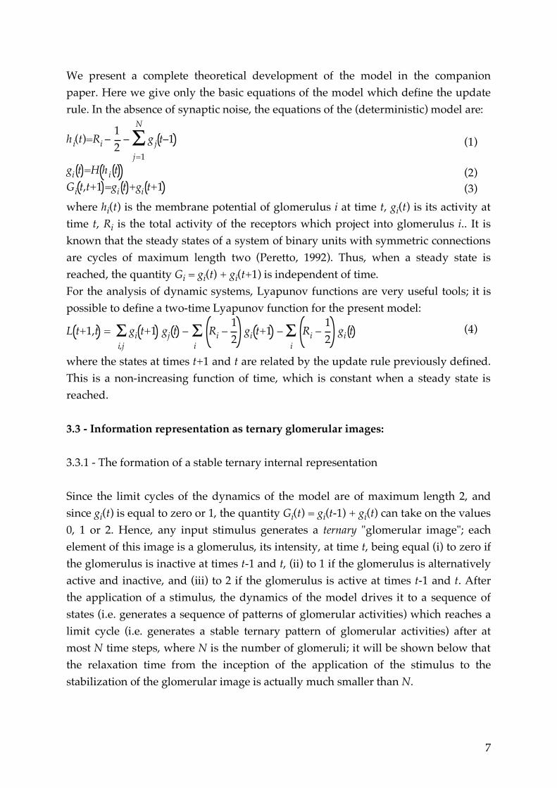
We present a complete theoretical development of the model in the companion paper. Here we give only the basic equations of the model which define the update rule. In the absence of synaptic noise, the equations of the (deterministic) model are:

hi(t)=Ri –1

2– gj t–1!

j=1

N

(1)

gi t =H hi t (2) Gi t,t+1 =gi t +gi t+1 (3)

where hi(t) is the membrane potential of glomerulus i at time t, gi(t) is its activity at time t, Ri is the total activity of the receptors which project into glomerulus i.. It is known that the steady states of a system of binary units with symmetric connections are cycles of maximum length two (Peretto, 1992). Thus, when a steady state is reached, the quantity Gi = gi(t) + gi(t+1) is independent of time. For the analysis of dynamic systems, Lyapunov functions are very useful tools; it is possible to define a two-time Lyapunov function for the present model:

L t+1,t = gi t+1 gj t – Ri –

1

2gi t+1!

i

– Ri –1

2gi t!

i

!i,j

(4)

where the states at times t+1 and t are related by the update rule previously defined. This is a non-increasing function of time, which is constant when a steady state is reached. 3.3 - Information representation as ternary glomerular images: 3.3.1 - The formation of a stable ternary internal representation Since the limit cycles of the dynamics of the model are of maximum length 2, and since gi(t) is equal to zero or 1, the quantity Gi(t) = gi(t-1) + gi(t) can take on the values 0, 1 or 2. Hence, any input stimulus generates a ternary "glomerular image"; each element of this image is a glomerulus, its intensity, at time t, being equal (i) to zero if the glomerulus is inactive at times t-1 and t, (ii) to 1 if the glomerulus is alternatively active and inactive, and (iii) to 2 if the glomerulus is active at times t-1 and t. After the application of a stimulus, the dynamics of the model drives it to a sequence of states (i.e. generates a sequence of patterns of glomerular activities) which reaches a limit cycle (i.e. generates a stable ternary pattern of glomerular activities) after at most N time steps, where N is the number of glomeruli; it will be shown below that the relaxation time from the inception of the application of the stimulus to the stabilization of the glomerular image is actually much smaller than N.

8

To summarize, if an input stimulus is applied for a period of time larger than the relaxation time, a stable ternary glomerular image arises, which can be regarded as a stable spatio-temporal internal representation of the stimulus; this internal representation is not unique: since the model is dynamic, it depends on the initial state of the model at the application of the stimulus; therefore, the present model is suitable for the processing of sequences of inputs, which is essential for understanding the response to the fluctuating odorant signal. 3.3.2 - The relationship between the stimulus and the ternary representation The stimulus which is input to the glomerular level is a vector of N activities of the N families of receptors; each of these activities can be regarded as being proportional to the number of active receptor cells of the corresponding family; thus, we model the input of the glomerular level as a vector of N positive integers. The signal processing performed by the model leads to a stable ternary image of N elements; thus, the model performs a mapping from a space of N positive integers, with an infinite number of vectors, to a space with only 3N possible vectors. It will be shown in the companion paper that the ternary olfactory imagecan be regarded as the image obtained by thresholding the signal which is input to the glomeruli by two thresholds which are the same for all glomeruli, but which depend on the input signal. Each attractor is thus uniquely characterized by a pair of thresholds; it will be further shown that these thresholds are directly related to the number of active glomeruli at each time step of the limit cycle. The contrast enhancement thus obtained is a classical result of the presence of lateral inhibition; in the present model, this thresholding is dynamic: the thresholds are not fixed in advance, but they depend both on the input stimulus and on the initial state of the system.For graphical purposes, the input vector of integers can be represented either as a bar graph or as an image with N grey levels. This is illustrated on Figure 2: the input is {3 0 5 2 1}; one of the possible stable glomerular images resulting from the application of this stimulus is {1 0 2 1 0}, which is the sum of the two alternating states of the limit cycle {0 0 1 0 0} and {1 0 1 1 0}; the number of active glomeruli is S1 = 1 in the first state and S2 = 3 in the second state; it can be easily checked on Figure 2 that the ternary glomerular representation is obtained by thresholding the input image with two thresholds θ1=1+1/2 = 1.5 and θ2=3+1/2 = 3.5.

It is shown in the companion paper that, given a stimulus, all the possible glomerular images can be found analytically (without resorting to numerical simulations which are subject to combinatorial explosion); in addition, the probability of occurrence of

9

each of these images, given a probability distribution of the initial states, can also be computed analytically. An example of such results is shown on Figure 3. 3.4 - Modeling the synaptic noise: In the previous section we have considered the noise-free dynamics of the model. In the present section, all the possible stochastic phenomena in the biological network are modeled in the following, classical way (Peretto, 1992): each glomerulus is assigned a firing probability which is a sigmoid function of its membrane potential. The slope of the sigmoid decreases with the noise, and becomes infinite at zero noise: this corresponds to the Heaviside activation function of the glomeruli in the deterministic version of the model. In the companion paper, we prove that the noisy system "searches" for the minimum value of the Lyapunov function defined above (4): in other words, if the model is left to evolve, with constant stimulus and decreasing noise, it will reach, among the possible glomerular patterns corresponding to this input in the noiseless regime, the glomerular image for which the Lyapunov function has the smallest value. The model thus "forgets" the initial state at the inception of the stimulation. In the example of Figure 3, a synaptic noise, however small, favors glomerular image number 2, for which the Lyapunov function has the smallest value. This result is an extension, to dynamic systems with stable limit cycles of length 2, of the well known effect of noise on dynamic systems whose stable states are fixed points. Thus, synaptic noise allows the model to escape from the limit cycles which are local minima of the Lyapunov function in the noise-free regime. 4 - PROPERTIES OF THE MODEL 4.1 - Properties of the model without synaptic noise: emergence of internal representations and extraction of key features from stimuli 4.1.1 - Internal representation and discrimination As a consequence of the reduction of the amount of information present in the ternary glomerular pattern of activity with respect to the information present in the inputs, a given internal representation at the glomerular level may arise from a very large number of inputs; typically, in the models with 17 glomeruli used in the

10

illustrative examples throughout the paper, the number of effective different inputs1 is 1917 which is on the order of 1021, whereas the number of possible glomerular patterns of activity is 317 which is on the order of 109. This is typical of a pattern recognition system, which uses successive information reduction processes until the recognition can be completed. The crucial question is: on what basis is this information reduction performed ? Since lateral inhibition plays an important role in our model, it is natural to conjecture that the information reduction is performed on the basis of contrast between receptor activities. Actually, one of the specific features of our model is the fact that the derivation of all inputs that may give rise to a given pattern of glomerular activity can be done analytically, and that the total number of input images giving rise to a given glomerular image can be readily computed. Figure 5 illustrates this point by showing a few inputs that give rise to a given stable ternary image. Billions of very different inputs may give rise to the same pattern of glomerular activity provided that they have some common features, as will be shown below. Although the present model performs information reduction in a very efficient way, it still has discrimination properties: two signals which are very similar may generate quite different glomerular images. Figure 6 illustrates such a situation. To summarize, the present model has the ability of building internal representations on the basis of the relative intensities of the activities of the receptors, and these internal representations still allow the discrimination between different inputs. If we assume that a training process exists at the level of the piriform cortex, which allows the storage of internal representations, then the system has both discrimination and generalization properties. 4.1.2 - Processing of sequences: key feature extraction and stabilization. Thus far we considered the response of a system to a constant input in the steady state, i.e. once a stable pattern of activity is reached at the glomerular level. We investigate now the whole dynamics of the response, in three situations: (i) the input is constant in time. (ii) the input is a sequence of inputs with common features. (iii) the input is a sequence of inputs without common features.

1 Since the glomerular image is obtained, as explained in section 3.3.2, by thresholding the input with thresholds between zero and N, all inputs larger than N+1 produce the same effect; although the number of possible inputs is infinite, the effective number of inputs is thus (N+2)N.

11

Since we consider, at this point, the deterministic model (i.e. without synaptic noise) a constant input drives the system into a steady state which is a cycle of maximum length 2. The transient regime is of maximal duration N. This is illustrated on Figure 7, where, depending on the initial state, a given input gives rise to three different glomerular images, with three different relaxation times. We have seen in the previous section that a given glomerular pattern activation can be generated by a very large number of inputs on the basis of the amplitude of the receptor activities. Therefore, if a sequence of such inputs is presented when the corresponding glomerular image is already formed, then the latter will not change, irrespective of the fluctuations of the inputs, provided the latter comply with the threshold conditions that uniquely define the glomerular image. Hence, the model exhibits two properties which are essential in the context of olfaction: when presented with a sequence of inputs, the model extracts the key features (in terms of receptor activities) which are common to the stimuli of the sequence, if any, and, at the same time, produces a stable glomerular pattern of activity which codes for these common features. This property is clearly apparent on the example of figure 8: the sequence of inputs contains very different "images" at the receptor level, but, despite the fluctuations, common features are present in the whole sequence (high activity of receptor 7 and relatively low activity of receptors 14 and 17). After presentation of 7 different inputs, the system stabilizes a spatio-temporal pattern of activity featuring a constant high activity of glomerulus 7 and a constant quiescence of glomeruli 14 and 17. If the sequence contains random inputs without common features, the glomerular activity changes with each inputs and does not stabilize, as shown on Figure 9: no feature extraction occurs since nothing is there to be extracted. In the example shown on Figure 8, the duration of the application of the stimulus is large enough (9 time units) that the steady state is reached before the next input of the sequence is applied. Interestingly, this is not a necessary condition for the model to find the stable glomerular image that codes for the key feature to emerge; moreover, it turns out that a rapid succession of stimuli may actually decrease the relaxation time to the stable glomerular pattern. This is shown on Figure 10: the same sequence of receptor patterns as in Figure 8 is presented, but the duration of the application of the stimuli is only 3 time units; then the stable glomerular image appears after the application of the first three stimuli, whereas the application of the first seven stimuli was necessary in the simulation shown on Figure 8.

12

To summarize, we have shown on the examples presented in this section that the noise-free model provides a possible mechanism for the extraction of key features from the odorant signal and the emergence of stable glomerular images. In the next section, we show that these properties are preserved, and, to some extent, enhanced, when internal noise (such as synaptic noise) is present, and that additional interesting properties emerge. 4.2 - Properties of the model in the presence of synaptic noise In order to gain biological plausibility, we have to introduce in the model stepwise increases of complexity. The first of these steps consists in taking internal noise into account (we have seen in the previous section that the model is intrinsically robust to input noise). We show in the companion paper that the Markov chain formalism is a powerful tool to derive the steady probability distributions of the glomerular images, given the inputs, as a function of the noise. In this section we only present and analyze the results of simulations. As before, we consider the three following situations: (i) the input is constant in time, (ii) the input is a sequence of inputs with common features, (iii) the input is a sequence of inputs without common features, and we show that the properties of the model depend on the noise regime, as defined below.

We have seen that when an input is constant in time, one of several possible glomerular images emerges, depending on the initial glomerular pattern of activity. Since we model the effect of noise as a probabilistic firing of the neurons, stochastic variations of the glomerular activity may occur at each time step. If the noise level is low, the noise will cause slight stochastic variations around one of the stable glomerular images that would emerge in the absence of noise; specifically, it is proved in the companion paper that the glomerular image that appears in the presence of noise is, among the possible images that emerge in the absence of noise, the image for which the Lyapunov function of the model is minimum. Figure 11 illustrates such a situation: with the input and the initial state which lead the noise-free model to generate the third image in figure 7, we observe that this image actually appears at the beginning of the stimulation, but, another glomerular image appears soon, and remains stable with slight fluctuations. Among the three possible stable states, shown on Figures 3 and 7, which would arise in the noise-free regime, the image emerging in the presence of noise is the image whose activity pattern gives

13

rise to the smallest Lyapunov function (pattern 3 of Figure 3). To summarize, when a small noise is added to the model, two out of the three possible images can no longer be stable states: with the noise level considered in this experiment, irrespective of the initial state, the considered stimulus always gives rise to the same pattern of glomerular activity.

At higher noise levels, a different behavior appears. Figure 12 shows simulations with two different values of the noise parameter, and the corresponding mean glomerular activity profiles. In the first experiment, the glomerular activity, averaged over the duration of the stimulus, becomes closer to the average input activity (shown on Figure 11, top right) than to the stable activity pattern emerging at lower noise level (shown on Figure 11, bottom right); in the second simulation the mean glomerular activity is close to 1 for all glomeruli: the glomerular image approaches the garbage state mentioned in figure 9.

In order to get a quantitative view of the above results, we consider the euclidean distance between two images, an image being viewed as a vector with N components. Figure 13 shows the evolution of such distances with noise: (i) distance of the mean glomerular activity to the activity of the corresponding image without noise (minimum of the Lyapunov function), (ii) distance of the mean glomerular activity to the mean receptor activity, and (iii) distance of the mean glomerular activity to the "garbage state" where all glomerular activities are equal to 1.

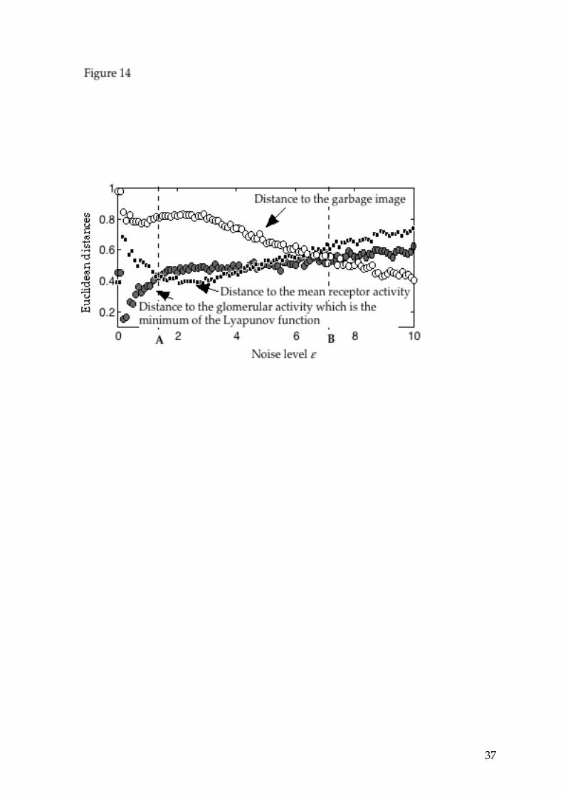
In view of the above results, three noise regimes can be defined: (i) the low noise domain, where the glomerular image fluctuates stochastically around the image which minimizes the Lyapunov function, whatever the initial glomerular activity; (ii) the medium noise domain, where the mean glomerular activity "copies" the receptor activities and (iii) the high noise domain, where the response is dominated by noise. In the noise domain where the distance between the glomerular image and the receptor activity is minimum, the system, although very non-linear, behaves almost linearly: the average response is essentially linear with respect to the input. If the input is a sequence of different inputs with common features, corresponding to the same minimum of the Lyapunov function, the distances previously defined can also be measured. The result is shown in figure 14: the three curves are very similar to those of figure 13, where a single input is applied at the receptor level. We also observe here the different noise regimes previously defined as well as the minimum

14

distance to the mean receptor activity at medium noise. Note that the condition for the emergence of a glomerular code is slightly more restrictive than in the noise-free case: the stimuli must have common features, and give rise to the same minimum of the Lyapunov function. Figure 15 shows the behavior of the glomerular image when there is a sequence of input and noise at the glomerular level: small and medium noises are considered. Finally, if a sequence of different stimuli without common features is applied, there is also a noise regime where the response is quasi-linear with respect to the receptor activity. To summarize, the effect of synaptic noise, modeled by a firing probability of the neurons, is the following : (i) in the noise-free case, the initial state of glomerular activity plays a crucial role in the determination of the stable glomerular image generated as a result of the application of the stimulus; when noise is present, the "memory" of the initial state is lost, so that the final distribution of glomerular activity depends solely on the stimulus; the mean glomerular activity is the activity which gives the minimal value to the Lyapunov function, if the duration of the observation is longer than the relaxation time necessary for reaching the steady state; (ii) in the noisy model, three different noise regimes may be defined; for a given number of glomeruli, their limits are independent on whether the stimulus is constant, or is a sequence of stimuli: - at low noise level, the steady state of the model gives rise to a glomerular image

which fluctuates around the image corresponding to the minimum value of the Lyapunov function given the input stimulus; thus, the two important properties of the system in the noise-free case - namely, the extraction of key features and the generation of a glomerular image which codes for the key features - are essentially preserved;

- at medium noise level, the mean glomerular activity tends to 'copy' the mean receptor activity; the model thus responds essentially linearly to the inputs, whether the latter have common features or not;

- at high noise, the input information is lost and the mean receptor activity is essentially a grey image.

5 - CONCLUSION AND FUTURE WORK

15

A dynamic model of the first two stages of the olfactory tract has been proposed, which provides a hypothetical neural mechanism for the extraction of key features and for the stabilization of a glomerular image despite the fluctuations present in the stimuli. The behavior of the model has been investigated both in the absence and in the presence of synaptic noise; simulation results have been presented, which show that the presence of synaptic noise produces two behaviors, depending on the noise level: at low noise, the properties are essentially the same as in the noise-free case, whereas at higher noise levels the glomerular pattern of activity becomes an image of the input of the glomerular stage; at still higher noise levels, the glomerular activity becomes uncorrelated to the inputs. Simulation results, however clear, are not proofs, especially in the field of nonlinear systems. The model which has been described in the present paper is fully tractable analytically, both in the presence and in the absence of noise. The companion paper provides general proofs of the properties described above. The present work should be regarded as an analytically tractable basis for future work directed towards increasing the biological plausibility of the model. One of the key issues is the introduction of different delays for different distances between glomeruli, thereby introducing a topology of the glomerular stage.

16

REFERENCES Ackers, R.P., Getz, W.M. (1993), "Response to Olfactory Receptor Neurons in

Honeybees to Odorant and their Binary Mixtures" J. Comput. Physiol, 173, 169-185. Axel, R. (1995), "The Molecular Logic of Smell", Scientific American, 273, 154-159. Bower, J. (1991),"Piriform Cortex and Olfactory Object Recognition", in Olfaction : A

model System for Computational Neuroscience, Davis J. & Eichenbaum H. (Eds), MIT Press, 265-285.

Fonta, C., Sun, X. J. and Masson, C. (1993), "Morphology and Spatial Distribution of

Bee Antennal Lobe Interneurones Responsive to Odours", Chemical Senses, 18, (2), 101-119.

Freeman, W. (1991), "Nonlinear Dynamics in Olfactory Information Processing" in

Olfaction : A model System for Computational Neuroscience, Davis J. & Eichenbaum H. (Eds), MIT Press, 225-249.

Hammer, M.(1997), "The Neural basis of Associative Reward Learning in

Honeybees" TINS, 20, pp 245-252 Hildebrand, J.G. (1995), " Analysis of Chemical Signals by Nervous Systems" Proc.

Natl. Acad. Sci. USA, 92, 67-74. Holley, A. (1994), "Les récepteurs des odeurs et autres attraits du modèle olfactif"

Médecine Sci., 10, 1077-1078. Holley, A., Sicard, G. (1994), "Les récepteurs olfactifs et le codage neuronal de

l'odeur"Médecine Sci., 10, 1091-1098. Hopfield, J.J. (1982), "Neural Networks and Physical Systems with Emergent

Collective Computational Abilities", Proc. Natl. Acad. Sci USA, 79, 2554-2558. Hopfield, J.J. (1991), "Olfactory Computation and Object Perception", Proc. Natl. Acad.

Sci. USA, 88, 6462-6466. Kerszberg, M. and Masson, C. (1995), "Signal Induced Selection Among Spontaneous

Oscillatory Patterns in a Model of Honeybee Olfactory Glomeruli", Biol. Cybern., 72, 795-810

17

Kauer, J. (1991), "Contributions of Topography and Parallel Processing to Odor Coding in the Vertebrate Olfactory Pathway", TINS, 14, (2), 79-85.

Laurent, G. (1996), "Odor Images and Tunes", Neuron, 16, 473-476. Laurent, G. (1996),"Dynamical Representation of Odors by Oscillating and Evolving

Neural Assemblies", TINS, 19 (11), 489-496. Laurent, G., Davidowitz H. (1994), "Encoding of Olfactory Information with

Oscillating Neural Assemblies" Science, 265, 1872-875. Linster, C., Masson, C. (1996) "A Neural Model of Olfactory Memory in the

Honeybee's Antennal Lobe", Neural Comp., 8, 94-114 Masson, C. and Linster, C. (1996), "Towards a Cognitive Understanding of Odor

Discrimination: Combining Experimental and Theoretical Approaches", Behavioural processes, 35, 63-82.

Masson, C. and Mustaparta, H. (1990), "Chemical Information Processing in the

Olfactory System of Insects", Physiological Review, 70, (1), 199-245. Masson, C., Pham-Delegue, M. H., Fonta, C., Gascuel, J., Arnold, G., Nicolas, G. and

Kerszberg, M. (1993), "Recent Advances in the Concept of Adaptation to Odours in the Honeybee, Apis mellifera L", Apidologie, 24, (3), 169-194.

Menzel, R., Hammer, M., Braun, G., Mauelshagen, J. and Sugawa, M. (1991),

"Neurobiology of Learning and Memory in Honeybees", in Behavioural and physiology of bees, L. J. Goodman and F. R.C., CAB Int.

Peretto, P. (1992), "An Introduction to the Modeling of Neural Networks", Cambridge. Pham-Delègue, M. H., Bailez, O., Blight, M., Masson, C., Picard-Nizou, A. L. and

Wadhams, L. J. (1993), "Behavioural Discrimination of Oilseed rape Volatiles by the Honeybee", Chem. Senses, 18, (5), 483-494.

Pham-Delègue, M. H., Masson, C. and Etievant, P. (1991), "Allochemicals Mediating

Foraging Behaviour : the Bee-sunflower Model", in Behaviour and physiology of bees, L. J. Goodman and R. C. Fisher, CAB Int.

Selzer, R. (1981), "The Processing of a Complex Food Odor by Antennal Olfactory

Receptors of Periplaneta americana."J. Comp. Physiol., 144, 509-519.

18

Shepherd, G. (1991), "Computational Structure of the Olfactory System", in Olfaction :

a model system for computational neuroscience, L. Davis and H. Eichenbaum, MIT Press.

Shepherd, G. (1994), "Discrimination of Molecular Signals by the Olfactory Receptor

Neurons", Neuron, 13, 771-790. Sun, X. J., Fonta, C. and Masson, C. (1993), "Odour Quality Processing by Bee

Antennal Lobe Interneurones", Chemical Senses, 18, (4), 355-377. Vareschi, E. (1971), "Duftunterscheidung bei der Honigbiene Einzelzell-Ableitung

und Verhaltungreaktion"Z. Vergl. Physiol., 75, 143-173.

19

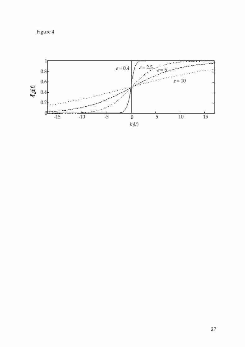
FIGURES CAPTIONS Figure 1: A network with N=3 units (a unit is indicated by a dotted frame: it consists of a glomerulus with its own receptor). The connections between a receptor neuron and its glomerular unit are excitatory with weight +1, whereas the connections between glomeruli (and self-connections) are inhibitory with weight -1. The membrane potential h of each glomerulus is the weighted sum of its inputs. The activation gi of glomerulus i is a Heaviside function of the potential hi in the deterministic version of the model. Figure 2: An example of the relationship between the input stimulus and the resulting ternary glomerular image in a noise-free model with N=5 units. We consider the input {Ri}={3 0 5 2 1}; in one of the possible limit cycles resulting from this stimulus, the following instantaneous glomerular activities alternate: {gi(t)}={0 0 1 0 0} and {gi(t+1)}={1 0 1 1 0}; when integrated on two time steps, they yield the network output: {Gi}={1 0 2 1 0}. The signal processing by this network is equivalent to the comparison between the activity level of each receptor and two thresholds, which are nothing but the number of active glomeruli at each time step of the cycle, namely S1=1 and S2=3, plus (1/2). Depending on whether the receptor activity is below θ1, between θ1 and θ2, or above θ2, the activity level of the corresponding glomerulus is equal to 0, 1 or 2. Figure 3: The possible internal representations of a given stimulus, and their probability of occurrence. The input and outputs are represented graphically in three ways: as a vector of integers, as a profile of activities or as a 'receptor image' with 19 grey levels for the inputs and three grey levels for the glomerular images. Depending on the initial state of the glomerular activities when the input {Ri} is applied, the contrast enhancements may be different: in the present case, three different pairs of thresholds may arise, leading to three different 'glomerular images'. The percentages indicated are the probabilities of occurrence of each spatio-temporal glomerular image, assuming that all initial states have equal probabilities. Figure 4: Noise is introduced in the model in such a way that the probability for a neuron i to be active attime t is given by equation

P gi t = 1 =1

1 + exp ! hi t / ", where ε is a

parameter which controls the amount of noise and ε = 0 corresponds to the

20

deterministic model. This equation replaces equation 2 for the update rule. The curves shown here represent this probability as a function of the membrane potential hi for various values of the parameter ε. Figure 5: In each frame an input is represented both by its profile and by its image in grey levels. The eight different stimuli of this example may give rise to the same pattern of glomerular activity. The profiles look very different, but these inputs have common features with respect to the dynamics they induce in the model: for example it appears clearly that the seventh receptor always has a "large" activity, while receptors 14 and 17 are relatively silent (receptors and glomeruli are numbered from top to bottom). The condition for an input to generate this particular output, which is characterized by the pair of thresholds (θ1 = S1+1/2=1.5, θ2 = S2+1/2 =15.5), can be expressed as follows : the activity of receptor 7 must be larger than θ2 =15.5, the activities of receptors 14 and 17 must be smaller than or equal to θ1=1.5, and the activity of the other receptors must belong to ]θ1=1.5, θ2=15.5]. For a model with N units, the number of inputs that satisfy these conditions is equal to

S1+1

N–S2 S

2–S

1

S2–S

1 N–S2+1

S1 . This number is on the order of 1017, i.e. approximately

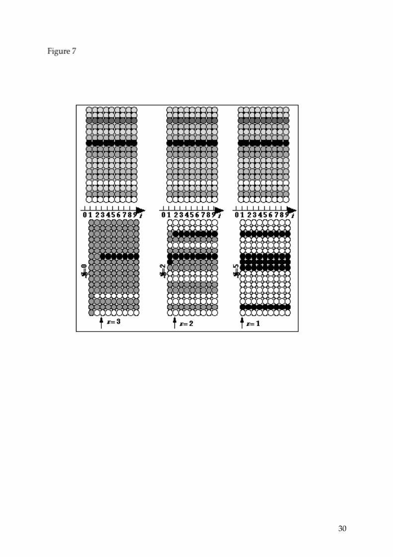
one input out of 104. Figure 6: Example of discrimination by the model. The profiles of the two inputs are very similar, but the possible emergent glomerular patterns of activity are different. Figure 7: Three different behaviors of the model with the same constant input. Top : activity of receptor cells as a function of time; bottom: resulting glomerular activity as a function of time, with three different initial states. The stimulus is kept constant for 9 time units. The glomerular image at time 1 results from the summation of the glomerular activities at times 0 and 1, the second image results from the summation of the glomerular activities on times 1 and 2, and so on. Depending on the number S0 of active glomeruli at time 0, three different stable glomerular patterns of activity are obtained (patterns shown on Figure 3), with different relaxation times τ. Figure 8:

21

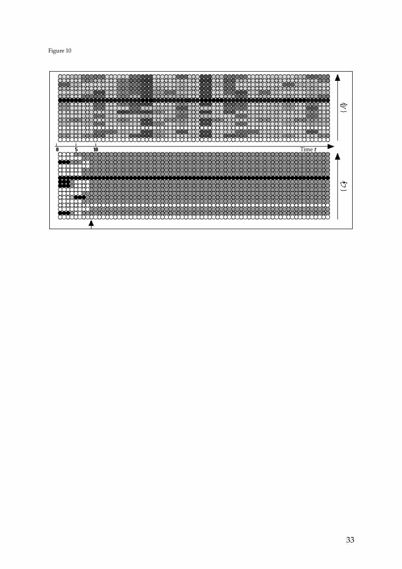
Response (bottom graph) of the model to a sequence of stimuli (top graph) having common features. Each stimulus is applied during 6 time steps; twelve different stimuli are presented in succession. Since the initial state is random, the model generates a first glomerular image, then after application of the second input, it reaches another attractor and so on; after the application of the seventh stimulus, the glomerular pattern finally "discovers" (this is indicated by an arrow) the common features of the seven patterns of receptor activities, and generates a stable glomerular image which codes for the underlying key features. Since subsequent stimuli of the sequence also exhibit the corresponding key features, the glomerular representation remains stable. Figure 9: As in figure 8, a sequence of different inputs is applied at the receptor level. The glomerular activity changes essentially at each change of the inputs; note that the image with a grey state for each glomerulus appears frequently: this state is a kind of garbage state, expressing the fact that no specific feature emerges. Figure 10: The inputs of this sequence are the same as those of figure 8, except for the fact that the duration of each stimulus is 3 time steps instead of 6 ; in the first 36 time steps they appear in the same order. The initial state is the same as in figure 8. The stable glomerular pattern that codes for the key features of the stimuli presented in the sequence emerges at the third input, earlier than previously. The image remains subsequently stable despite the fluctuations at the receptor level. Figure 11: In the noise-free regime, the stimulus and the initial glomerular activity (S0=5) would generate the third glomerular image shown on Figure 7 (pattern 1 of Figure 3). In the present simulation (with noise parameter ε=0.4) the output clearly converges to another activity pattern (pattern 2 of Figure 3), for which the Lyapunov function is minimum. This pattern appears after a relaxation time indicated here by the arrow. During the stimulation this image is impaired by noise, but the mean activity pattern of the glomeruli (averaged over the duration of the stimulus), shown at the bottom right of the graph, is very close to the activity pattern of the glomerular image without noise, shown as pattern 2 of Figure 3.

22

Figure 12: Glomerular patterns of activity in response to the same stimulus, with the same initial state, as shown on Figure 11, with noise parameters ε=2.5 (top graph) and ε=10 (bottom graph). In the top graph, the mean glomerular activity is close to the mean activity of the receptors (shown on Figure 11, top right); in the bottom graph, the mean glomerular activity becomes close to 1, independent of the stimulus. Figure 13: Evolution of the euclidean distance between the mean glomerular activity and (i) the mean receptor activity, (ii) the coding image, (iii) the garbage image, with increasing noise (increasing values of ε), for a constant input (shown on Figure 11) during 720 time steps, with the initial state shown on Figure 11. In the absence of noise, the stable glomerular image would be pattern 1 of Figure 3; therefore, there is a discontinuity of the distance to the activity corresponding to the minimum of the Lyapunov function: even with a very small noise, the system escapes from the metastable pattern to generate the pattern that minimizes the Lyapunov function. When the noise level increases, the distance to the minimum of the Lyapunov function increases, whereas the distance to the mean receptor activity decreases. This graph suggests the definition of three noise regimes (i) low noise (left of dotted line A), where the glomerular pattern of activity is essentially the minimum of the Lyapunov function, (ii) medium noise (between dotted line A and dotted line B), where the glomerular pattern of activity is closer to the mean receptor activity than to the minimum of the Lyapunov function, (iii) high noise (right of dotted line B), where the glomerular activity is dominated by noise and becomes essentially independent of the stimulus. Figure 14: Evolution of the euclidean distance between the mean glomerular activity and (i) the mean receptor activity, (ii) the coding image, (iii) the garbage image, with increasing noise (increasing values of ε), for a sequence of 12 stimuli with common features. Each input is stable during 60 time steps. The different noise regimes are separated by dotted lines. Figure 15: Response to a sequence of different stimuli with common features (top graph, same sequence as in figure 8) for two noise levels: low noise (ε=0.4, middle graph) and medium noise (ε=2.5, bottom graph). The activity profiles show that low noise generates a glomerular activity close to the image corresponding to the minimum of

23

the Lyapunov functions, and medium noise generates a glomerular activity which is closer to the mean receptor activity. Note that the addition of a small noise allows the system to find the key features earlier than it does in the absence of noise (compare to Figure 8).

24

!

R1

g1

!

R2

g2

!

R3

g3

Input {Ri}

Receptor layer

Output {Gi = gi(t) + gi(t+1)}

Glomerular layer

Figure 1

FIGURES

25

+

S1 = 1 S2 = 3

!1 = 1.5

!2 = 3.5{ Ri }

3 0 5 2 1

{ Gi }

1 0 2 1 0

{ gi (t)} { gi (t+1)}

3 50 2 1

1 0 2 1 0

"

Input

Output

0

1

2

0

2

4

! = S + 0.5

Figure 2

26

27

28

29

30

31

32

33

34

35

36

37

38

{Ri}

{Gi}

Time t

{Gi}

Figure 15