a dynamical theory of brownian motion for the rayleigh...

Journal of Statistical Physics, Vol. 47, Nos. 5/6, 1987

A Dynamical Theory of Brownian Motion for the Rayleigh Gas

D o m o k o s Szfisz 1 and Bfilint T6th 1

Received November 10, 1986

A dynamical theory of the Brownian motion is worked out for the Rayleigh gas and open problems of this theory are surveyed.

KEY WORDS: Diffusion limit; Brownian motion; mass and space-time scaling.

1. I N T R O D U C T I O N

Recent progress (1'I4'17'18) has again raised hopes of understand the dynamical theory of Brownian motion for simplified models at least. In fact, Ref. 18 formulates such a theory for the Rayleigh gas, i.e., for the case when the Brownian particle interacts with an ideal gas (cf. Ref. 16). Moreover, mathematical results were also obtained supporting the theory.

The aim of the present paper is to explain the main ideas of the aforementioned paper in order to understand which open problems of the theory seem realistic and, roughly speaking, what kind of difficulties should be overcome in their solution.

To prepare the exposition of the theory (presented in Section 4), we give a mathematical formulation of the model in Section 2 and survey some previous results in Section 3. The main components of the sketchy proof outlined in Section 5 are explained in Sections 6 (the Markovian approximation) and 7 (the coupling). Finally, Section 8 surveys the most interesting open problems of the theory for both the one- and multi- dimensional cases (apart from this last point, we restrict ourselves to the 1D case).

Mathematical Institute of the Hungarian Academy of Sciences, Budapest, H-1364, Hungary.

681

0022-4715/87/0600-0681505.00/0 �9 1987 Plenum Publishing Corporation

682 Sz&sz and Tbth

2. F O R M U L A T I O N OF THE M O D E L

A one-dimensional system of point particles consists of a tagged particle of mass M (the Brownian particle) interacting with an infinite ideal gas of particles of mass 1 (light particles). The dynamics of the system is governed by the laws of classical mechanics, assuming uniform motion plus elastic collisions between the Brownian particle and the light ones and no interaction among the light particles.

The collision rules are the following:

M - 1 2 2M M - 1 V + - V- v- v + = - V - - - v - (2.1)

- M + I + M~--i- ' M + I M + I

o r

2 2M A V = V + - V - = - ( V - - v - ) ; A v = v + - v - - ( V - v )

M + I M + I

where V + and v + are the post- (pre-) collision velocities of the colliding Brownian resp. light particle. The most convenient approach is to describe our system as seen from the Brownian particle (the so-called "Mfinchhausen picture"). In this picture the phase space is

X = [ R x ( 2 = {Z= (V, co): V ~ , co= (qi, vi)i~1~s }

where I is a countably infinite index set,/2 is the set of locally finite coun- table point systems in R x A, V is the velocity of the Brownian particle, and (qi, v~)~x are the coordinates (relative to the position of the Brownian particle) and the velocities of the light particles. We say that co is the environment seen by the Brownian particle./2 is a Polish space endowed with the natural a-algebra ~o generated by counting functions on compact sets. The ~-algebra on X is Y = ~ x Yo, ~ being the Borel algebra on R. The system is distributed according to the Gibbs measure

iiM(d( V, eJ) ) = dgM( V) . v(d(~)

with v the Poisson measure on (f2, ~ ) with intensity dx dFl(v) , and

dFM(V) = (M/Zz~) I/z exp(-MV2/2) d V ( M > 0)

Denote by S y the dynamics of the system. The following two facts are assumed to be known:

(a) For each M there exists a set ~M c 3Z of/~M-measure 1 on which the maps S~ M are well defined for any t~ ~, and S M , = SMoS M. (The equilibrium dynamics exists with probability 1.)

Brownian Motion for the Rayleigh Gas 683

(b) The group of transformations S f f : 3 i M ~ 3 1 M preserves the measure #M. The random variables to be introduced below are defined on different probabili ty spaces, depending on M.

We shall use the notations

V(Z) = V and co()0 = co iff Z = (V, co)E3;

v ~ ( z ) = v ( S T z ) , z ~ x M

Q f ( z ) = M v; ( z ) ds, z e X. ~

Throughout this paper W} ~ will denote a Wiener process of variance a z with W~0 ~ = 0, and for brevity we let W, = W} z).

The diffusion process ~/, satisfying the stochastic differential equation

dqt = -Ttl~ dt + D 1/2 dW~

is called an Ornstein-Uhlenbeck (velocity) process. If qo is distributed according to the Gaussian law with mean 0 and variance (27) -1 D, then r/, is a stationary Gauss -Markov process.

The integral process

fo 3, = tl ~ ds

is called the Ornstein-Uhlenbeck position process. We shall use these processes with the following choice of parameters:

y = (4/m)(2/7c) 1/2, D = (8 /m2) (2 /~ ) ~/2

and we will use the notations q},-/ and ~I m) for them (m is a positive constant). It is worth mentioning that if 7 ~ 0% D ~ ov in such a way that D7 -2 ---~dzE [~+, then the Ornstein-Uhlenbeck position process ~, converges in distribution to a Wiener process W (~) (see Ref. 11). Thus,

~I m) ~ ml -~ as m ~ 0 (2.2)

with ~r 2 = (~z/8) 1/2.

3. S U R V E Y OF S O M E R E S U L T S

Our final aim is to give a complete asymptotic description of the random processes

Q~(A)/A1/2 as A ~ oo

684 Szbsz and T6th

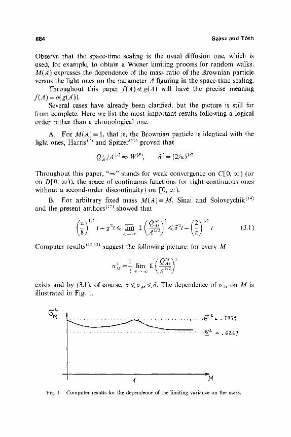
Observe that the space-time scaling is the usual diffusion one, which is used, for example, to obtain a Wiener limiting process for random walks. M(A) expresses the dependence of the mass ratio of the Brownian particle versus the light ones on the parameter A figuring in the space-time scaling.

Throughout this paper f (A)~ g(A) will have the precise meaning f(A ) = o(g(A)).

Several cases have already been clarified, but the picture is still far from complete. Here we list the most important results following a logical order rather than a chronological one.

A. For M(A) - 1, that is, the Brownian particle is identical with the light ones, Harris (y) and Spitzer (15) proved that

QI.IA1/2~ W(<~), e i a= (2/zc) 1/2

Throughout this paper, " ~ " stands for weak convergence on C[0, oo) (or on D[0, oo)), the space of continuous functions (or right continuous ones without a second-order discontinuity) on [0, oo).

B. For arbitrary fixed mass M(A)=M, Sinai and Soloveychik/14) and the present authors (17) showed that

Computer results (1z'13) suggest the following picture: for every M

cr2= 1 lim ~_{Q~,~2

exists and by (3.1), of course, a~<crM~<& The dependence of cr M on M is illustrated in Fig. 1.

. . . . . . . . . . . ~ = . 7 9 7 = /

. . . . . . . . . . . . . . . . . . . . . . . . . . . . . . . . . . c : . : . . . . 6-~- = . a Z # 7

4 N

Fig. 1. Computer results for the dependence of the limiting variance on the mass,


C. From the proofs of Ref. 17 it is easy to see that, in (2.3), the upper bound holds for an arbitrary scaling functional M(A), while the lower bound holds whenever M ( A ) = o(A).

D. For M ( A ) = m . A , me(O, c~), Holley (8) proved that

AI/ZV~.A ~ ~](m); Q,j.A/Am ~ ~(m)

Important Remark. The results B and D can be linked by observing that Ecf. (2.2)]

~(m) ~ W(O) as m --+ O

4. THE T H E O R Y

On the basis of the aforementioned results, we expect the following complete asymptotic picture.

1. Case M(A) --> 0:

2. Case M ( A ) = M :

QM(A)/A 1/2 ~ W(~)

Q~./A ~/2 ~ T M, g ~ ffM ~

where T M, M > 0, are random processes with stationary increments and with asymptotic variance a~ .

We know that T I = W ~, while simulations support that aM--)_a as M --+ c~ and aM --* a as M ---) 0 (the result for M - 1 was proved in Refs. 7 and 15, while the bounds on the variances were given in Refs. 14 and 17).

3. Case I ~ M ( A ) < A :

Q~.(a)/A !./2 ~ W(_O-)

4. Case M(A) = mA:

where ~(') is introduced in Section 2. This convergence was proved in Ref. 8. For rn ---) 0, (2.2) holds. For m --+ ~ , ~(m) ~ 0.

5. Case M ( A ) ~ A:

Q~.(A)/A 1/2 =~ 0 (trivial)

822/47/5-6-6

686 Szbsz and T6th

Of course, this case is not trivial if we allow spatial rescalings different from A 1/2. Indeed, by an application of a theorem of Kurtz (essentially by the same method as that used in Ref. 8), we find the correct asymptotics

A 1/2 v~(A)_ 1 {[M(A)]m vM(A)}I/2 ~_~..~tA

[M(A)] 1/2

where [M(A)] 1/2 V M(A) has a standard Gaussian distribution and ~A converges in distribution to a Wiener process of variance 4(2/~) ~/2. (If d > 1, a similar statement holds with a limiting variance depending on the dimension. )

One further step in completing the picture outlined above is the following.

Theorem 1. IfAI/2+~<M(A)~A ( e > 0 ) , t h e n

Q~.(A)/A 1/2 ~ W(,,I

5. S K E T C H OF P R O O F OF T H E O R E M 1

The first--and in a sense principal--difficulty in the dynamics of the Brownian particle is the non-Markovian nature of its motion. Indeed, light particles between their first and last collisions with the Brownian one carry information on past collisions in a complicated way. Nonetheless, it is a natural idea to consider a Markov process whose evolution mimics the physical process; this Markov process, of course, disregards recollisions that could spoil its Markovian nature. This Markov version can help both on an intuitive level, to give a feeling for what the mechanical process is like, and on a technical level, if we can construct a good coupling between the mechanical and the Markov processes. To our knowledge, this idea was first used in a rigorous argument by Holley (8) (cf. case D, Section 3) and our proof is also a realization of this strategy.

Let us first construct a family of Markov processes Vf , M > 0, closely related to the mechanical velocity processes Vf. In words, the p M are defined as follows: we imagine that the environment is recreated after each collision corresponding to the time-invariant distribution v. Thus, the Markovian velocity process ~'~ is a pure jump process on ~ with jump rates

Rate ( M--1 m ~ ) 1 ~2/21V-vldv V~M+--------f V+ v = ~ e


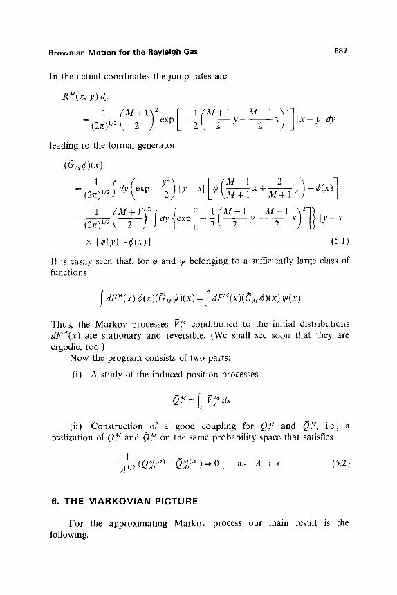
In the actual coordinates the jump rates are

RM(x, y) dy

- ~ ) exp - y x Ix-yldy

leading to the formal generator

(SMO)(x) 2 2

- (2~z~77 t l dy ( exP-2 ) lY-Xl[~(M-lx+-M--~y)-~(x)]\-~-~

_ 1 ( M 2 1)2 {exp I(M2---~lv-M----~I

x D ( y ) - ~(x)] (5.1)

It is easily seen that, for ~b and ~, belonging to a sufficiently large class of functions

f dFar ~b(x)(CM~)(x)= f dFM(x)(GMO)(x) t~(x)

Thus, the Markov processes Vff conditioned to the initial distributions dF~(x) are stationary and reversible. (We shall see soon that they are ergodic, too.)

Now the program consists of two parts:

(i) A study of the induced position processes

(ii) Construction of a good coupling for Q~ and Q, a4, i.e., a realization of Q~ and OM on the same probability space that satisfies f

1 (Q~(a)_ O~(a)) ~ 0 as A + m (5.2)

A 1/2

6. T H E M A R K O V I A N P I C T U R E

For the approximating Markov process our main result is the following.

688

with

and

T h e o r e m 2. (i)

Sz&sz and T6th

(Fixed masses). For any fixed M~ (0, ao)

O_~./A 1/2 ==:> W(#M)

8 2 ) ( 1 + 1/M)~/2 _a 2

lim 82 =g2 m ~ c o

(ii) (Sublinearly increasing masses). If 1 ~ M ( A ) ~ A, then

O~. (4)/A 1/2 ~ W(O-)

In fact, our methods give the following complete asymptotic charac- terization of the induced position processes ~)~ (the reader is encouraged to compare it with the analogous picture formulated for Q~ in the preceding section).

1. Case M ( A ) ~ O :

2. Case M ( A ) = M:

Q~.(A)/AI/2 is not tight

O~4.(AI/A i/2 =:> W(ff.,,,4)

with 8 2 ~ M 1/2 f o r M - ~ 0 a n d f f 2 ~ g 2 a s M ~ o o .

3. Case 1 ~ M ( A ) ~ A :

O~.(A)/A 1/2 ~ W(Zl

4. Case M(A) = mA:

5. Case M ( A ) ~ A:

O~(A~/A 1/2 ~ 0

Cases 1-3 follow from Theorem 2; Case 4 is proved in Ref. 8; Case 5 is trivial.

It is instructive to compare the pictures for the mechanical versus the Markovian processes (Table I).


Table I

A -I /2Q~(A)=, A - , / 2 ~ . I A )

d = !

Expected Prove& Proved ~

M( A ) ,4 1 W ~ ?? Explodes

M ( A ) ~ M T M ?? W e~'~

aM --~ a if M ~ oo Only known~14'17): Also known: o- ~< O-M ~< ff ~ 2 ~ M - i / 2 (M ---, 0)

6 ~ t ~ o -2 ( m ~ 00) ~ >>. (1 + 1 /M) I/2 a ~

1 " ~ M ( A ) ~ A W '~ ?? W ~ Known if M ( A ) >> A ll2 +

M ( A ) = m A ~" Ref. 8 ~" (Ref. 8)

M ( A ) >> A 0 Trivial 0

u Proved results without a reference are contained in Ref. 18.

Denote IF',M = ~,~I~tl/2 ~'M--M," Then

A ,/~,,SM~,,, _- (A/M) ~'~ (,,,/M F'f ds ~0

are additive functionals of stationary, reversible Markov processes with a common invariant measure, namely the standard Gaussian one. Consider now the Hilbert spaces

�9 Y{~' = L2(~, (M/2~) 1/2 e _M:,2/2)

and introduce the unitary isomorphisms UM: ~ M ~ ~r by (UM(b)(x) = ~(x/Ml/2) . Then (~M acts in ~ M , while the generator of lT"y is MGM acting in idol, where GM = U~tGM(UM) - t . The proof of Theorem 2 relies upon a lemma ensuring the uniform (in M) ergodicity of the Markov processes ~'y in a rather strong sense.

Gap Lemma. [ f l ~ < M < o o , then

S p e c ( M G M ) c~ M + 1

This uniform ergodicity is combined with a martingale approximation, which is a useful tool to obtain central limit theorems for additive

690 Szbsz and T6th

functionals of Markov processes. (4'6'9) In fact, part (i) of Theorem 2 follows directly from Ref. 6 with the exact limiting variance

5 2 = -2(~b, (MGM) - t 45)a~, where ~ ( x ) = x

Part (ii), however, requires additional arguments, since we have a double array of Markov processes in this case.

7. C O U P L I N G

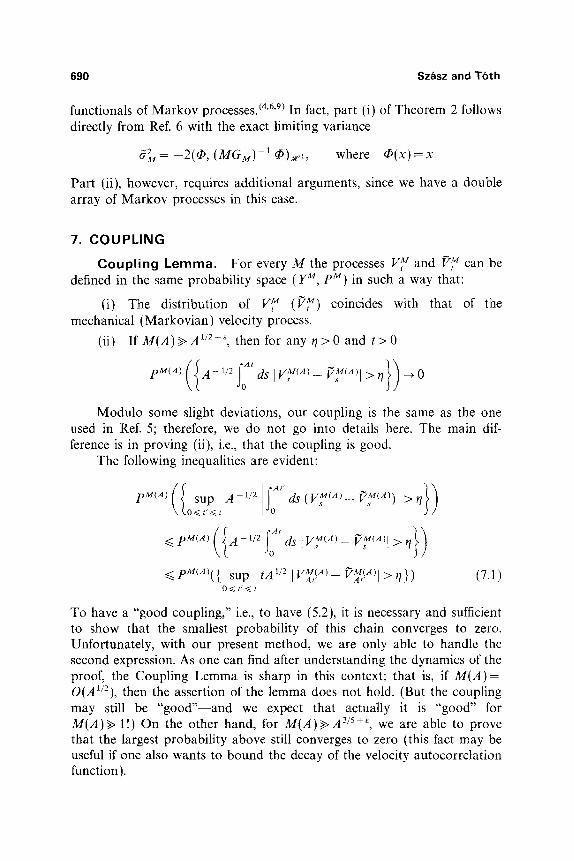
Coupl ing Lemma. For every M the processes V~ and ~'~ can be defined in the same probability space (Y~, pM) in such a way that:

(i) The distribution of V~ (V~) coincides with that of the mechanical (Markovian) velocity process.

(ii) I fM(A)>>A 1/2 + ~, then for a n y r / > 0 a n d t > 0

pM(A~ A-l/: ds IVy ~A~- PY(~I > ~ - , 0

Modulo some slight deviations, our coupling is the same as the one used in Ref. 5; therefore, we do not go into details here. The main difference is in proving (ii), i.e., that the coupling is good.

The following inequalities are evident:

({ }) p M ~ sup A 1/2 d s ( V s ~ ( ~ - f ' y (A~) >rl O<~t'<~t

~ pM(A~({ sup tA '/2 IVy! A I - P~:~>l >~}) (7.1) O <~ t' <~ t

To have a "good coupling," i.e., to have (5.2), it is necessary and sufficient to show that the smallest probability of this chain converges to zero. Unfortunately, with our present method, we are only able to handle the second expression. As one can find after understanding the dynamics of the proof, the Coupling Lemma is sharp in this context; that is, if M ( A ) = 0(A1/2), then the assertion of the lemma does not hold. (But the coupling may still be "good"--and we expect that actually it is "good" for M(A)>> 1!) On the other hand, for M(A)>~A 3/5+~, we are able to prove that the largest probability above still converges to zero (this fact may be useful if one also wants to bound the decay of the velocity autocorrelation function).


The fundamental idea in the construction of a good coupling is that the processes V~ and ~'~ should suffer as many joint collisions with light particles as possible. Our main observations are:

(a) These joint collisions have a contractive effect for the difference of the velocities, as is easily seen from the collision equations (similar ideas were heavily used in Ref. 1 ).

(b) To obtain a good bound for the L1 deviation of the velocity processes, one does not need to add up the effects of all collisions, but it is sufficient to use certain integrals of exponentially decaying functions incor- porating the contractive effects of (a).

8. P R O B L E M S

8.1. O n e - D i m e n s i o n a l Case

The question marks in Table I represent the main areas of problems. We consider them in more detail.

8.1.1. C a s e M ( A ) ~ 1. Since the conjecture A-t/2Q~(A)~ W e, if A-- .ov and M(A)--*O, comes from a simple intuitive perturbative argument, it is reasonable to first look for a rigorous perturbative proof to show that

lim A -1 Var QM(A) = 62 A ~ o ~ , M ( A ) ~ O

8.1.2. C a s e M ( A ) - M . (a) It is an extremely intruguing question whether, in general, T M is a Wiener process or not. Computer results by Sinai's group (1~) suggest that, for general M, it is not. On the other hand, other computer results (12) also gave the c(M)o t -3 asymptotic decay of the velocity autocorrelation EVoMV, M that had been known for the Wiener case M - 1. (I~

(b) The solution of the previous problem seems hopeless at present, since, for example, no good coupling exists; therefore we expect further progress in more modest directions, e.g., our estimates for ffM may be of some use in bounding a M for large M and to show first that aM < ff if M is large. It is more difficult to show that the relations limM~ ~ a M = g , limM~ ~ aM=l im~t~0 aM = 6 suggested by the numerical results hold.

8.1.3. C a s e 1 ~ M(A) ~ A ~/z + ~ At present we have no device to catch the cancellations that occur in the smallest probability of (7.1) by symmetry reasons. Here a clever argument may help, and to expect further progress is realistic.

692 Sz&sz and T6th

Table II

A -1/2Q~.~)~ A 1/2QM.IA,

d > l

Expec ted P roved ~ P roved ~

M(A) ~ 1 ?? ?? Explodes M .,~t

M(A) =- M W~,R ?? W ~ aaMR ~> ffd, R ?? - -

1 ~ M(A) ~ A W -~'R ?? W -~'R Only if M(A ) ~> A z/2 +

" ~" (Ref. 5) M(A) = rnA ~d,R Ref. 5 ~d,R

M( A ) ~> A 0 Triv ia l 0 t r ivial

P roved results w i thou t a reference are con ta ined in Ref. 18.

8.2. Mult idimensional Case

Now an additional nontrivial parameter appears: the radius R = R(A) of the spherical Brownian particle. For simplicity, we suppose R ( A ) - R and then the possibilities are the same as those in the 1D situation. Before formulating the questions, we again compile the possibilities (Table II).

A Markov approximation ~M was defined in Ref. 5 and the arguments (the Gap Lemma and its consequences) of Ref. 18 extend to this case, too. Moreover, for M(A)=mA, Dfirretal. (5) constructed a good coupling to show that the limiting process is a d-dimensional Ornstein-Uhlenbeck one. The method of our aforementioned paper also gives a complete analog of Theorem 1 with the limiting variance aZ.R = R l-ed(~z/8).

8 .2.1. C a s e M ( A ) _ - - M . We expect a limiting Wiener process of variance (a~R) 2 for any d>~ 2, though a proof seems realistic for d~> 5 only, since then the memory decays sufficiently strongly so as to give hope that an inductive argument works. (2'3)

The conjectured inequality is an analog of the 1D one, but it is a further question whether a similar upper bound can be expected at all.

8.2.2. C a s e 1 ~ M(A) ~A. Same as in the 1D situation.

8.2.3. Asymptotic Independence of Two Brownian Par- ticles. Suppose that two extended spherical particles of equal masses M move in an ideal gas and collide elastically with each other and with the gas particles. Here the system cannot be considered in equilibrium, but we expect that for reasonable initial measures (e.g., the Brownian particles


start from Qff(0) and M 0 " Q2 ( ) , IQM(0)--QM(0)] >2R with Maxwellian velocities and the measure of the light particles is Gibbsian outside the domains occupied by the spheres) and for M(A)>> 1 the rescaled trajec- tories A-I/2[Qff~)(At)- QM~A)(0)], j = 1, 2, behave asymptotically in the same way as independent copies of processes prescribed by Table II.

REFERENCES

1. C. Boldrighini, A. Pellegrinotti, E. Presutti, Ya. G. Sinai, and M. R. Soloveychik, Ergodic properties of a semi-infinite one-dimensional system of statistical mechanics, Commun. Math. Phys. 101:363-382 (1985).

2. D. Brydges and T. Spencer, Self-avoiding walk in 5 or more dimensions, Commun. Math. Phys. 97:125-148 (1985).

3. R. L. Dobrushin, presented at IAMP congress (1986). 4. D. Diirr and S. Goldstein, Remarks on the central limit theorem for weakly dependent

random variables, in Stochastic Processes--Mathematics and Physics, S. Albeverio, P. Blanchard, and L. Streit, eds. (Springer, 1986).

5. D. Diirr, S. Goldstein, and J. L. Lebowitz, A mechanical model of Brownian motion, Commun. Math. Phys. 78:507-530 (1981).

6. M. I. Gordin and B. A. Lifschic, Central limit theorem for stationary Markov chains, Dokl. Akad. Nauk SSSR 239:766-767 (1978).

7. T. G. Harris, Diffusions with collisions between particles, J. Appl. Prob. 2:323 338 (1965). 8. R, Holley, The motion of a heavy particle in an infinite one dimensional gas of hard

spheres, Z. Wahrsch. Verw. Geb. 17:181-219 (1971). 9. C. Kipnis and S. Varadhan, A central limit theorem for additive functionals of reversible

Markov processes and applications to simple exclusion, Commun. Math. Phys. 104:1-19 (1986).

10. J. L. Lebowitz and J. K. Percus, Kinetic equations and density expansions, Phys. Rev. 155:48 (1967).

11. E. Nelson, Dynamical Theory of Brownian Motion (Princeton University Press, 1967). 12. E. Omerti, M. Ronchetti, and D. Dfirr, Numerical evidence for mass dependence in the

diffusive behaviour of the "heavy particle" on the line, J. Star. Phys. 44:339 (t986). 13. Ya. G. Sinai, Personal communication. 14. Ya. G. Sinai and M. R. Soloveychik, One-dimensional classical massive particle in the

ideal gas, Commun. Math. Phys. 104:423-443 (1986). 15. F. Spitzer, Uniform motion with elastic collisions of an infinite particle system, J. Math.

Mech. 18:973-989 (1969). 16. H. Spohn, Kinetic equations from Hamiltonian dynamics: Markovian limits, Rev. Mod.

Phys. 53:569 (1980). 17. D. Szfisz and B. T6th, Bounds on the limiting variance of the heavy particle, Commun.

Math. Phys. 104:445-455 (1986). 18. D. Szfisz and B. Tdth, Towards a unified dynamical theory of the Brownian particle in an

ideal gas, Commun. Math. Phys., to appear.

a dynamical theory of brownian motion for the rayleigh...

Documents