A Fast Unified Algorithm for Solving Group-Lasso

Penalized Learning Problems

Yi Yang and Hui Zou∗

This version: July 2014

Abstract

This paper concerns a class of group-lasso learning problems where the objective

function is the sum of an empirical loss and the group-lasso penalty. For a class of loss

function satisfying a quadratic majorization condition, we derive a unified algorithm

called groupwise-majorization-descent (GMD) for efficiently computing the solution

paths of the corresponding group-lasso penalized learning problem. GMD allows for

general design matrices, without requiring the predictors to be group-wise orthonormal.

As illustration examples, we develop concrete algorithms for solving the group-lasso

penalized least squares and several group-lasso penalized large margin classifiers. These

group-lasso models have been implemented in an R package gglasso publicly available

from the Comprehensive R Archive Network (CRAN) at http://cran.r-project.

org/web/packages/gglasso. On simulated and real data, gglasso consistently out-

performs the existing software for computing the group-lasso that implements either

the classical groupwise descent algorithm or Nesterov’s method.

∗School of Statistics, University of Minnesota, Email: zouxx019@umn.edu.

1

Keywords: Groupwise descent, Group Lasso, grplasso, Large margin classifiers, MM prin-

ciple, SLEP.

1 Introduction

The lasso (Tibshirani, 1996) is a very popular technique for variable selection for high-

dimensional data. Consider the classical linear regression problem where we have a contin-

uous response y ∈ Rn and an n × p design matrix X. To remove the intercept that is not

penalized, we can first center y and each column of X, that is, all variables have mean zero.

The lasso linear regression solves the following ℓ1 penalized least squares:

argminβ

1

2∥y −Xβ∥22 + λ∥β∥1, λ > 0. (1)

The group-lasso (Yuan and Lin, 2006) is a generalization of the lasso for doing group-wise

variable selection. Yuan and Lin (2006) motivated the group-wise variable selection problem

by two important examples. The first example concerns the multi-factor ANOVA problem

where each factor is expressed through a set of dummy variables. In the ANOVA model,

deleting an irrelevant factor is equivalent to deleting a group of dummy variables. The second

example is the commonly used additive model in which each nonparametric component may

be expressed as a linear combination of basis functions of the original variables. Removing

a component in the additive model amounts to removing a group of coefficients of the basis

functions. In general, suppose that the predictors are put into K non-overlapping groups

such that (1, 2, . . . , p) =∪K

k=1 Ik where the cardinality of index set Ik is pk and Ik∩Ik′ = ∅

for k = k′. Consider the linear regression model again and the group-lasso linear regression

2

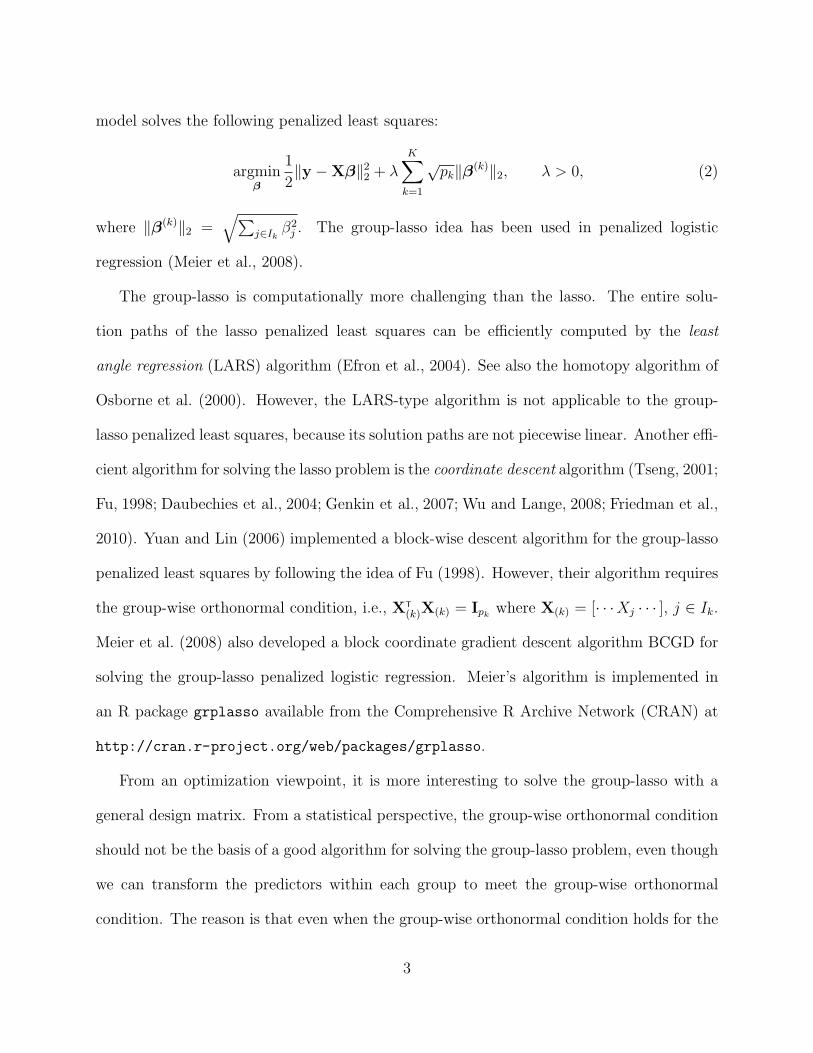
model solves the following penalized least squares:

argminβ

1

2∥y −Xβ∥22 + λ

K∑k=1

√pk∥β(k)∥2, λ > 0, (2)

where ∥β(k)∥2 =√∑

j∈Ik β2j . The group-lasso idea has been used in penalized logistic

regression (Meier et al., 2008).

The group-lasso is computationally more challenging than the lasso. The entire solu-

tion paths of the lasso penalized least squares can be efficiently computed by the least

angle regression (LARS) algorithm (Efron et al., 2004). See also the homotopy algorithm of

Osborne et al. (2000). However, the LARS-type algorithm is not applicable to the group-

lasso penalized least squares, because its solution paths are not piecewise linear. Another effi-

cient algorithm for solving the lasso problem is the coordinate descent algorithm (Tseng, 2001;

Fu, 1998; Daubechies et al., 2004; Genkin et al., 2007; Wu and Lange, 2008; Friedman et al.,

2010). Yuan and Lin (2006) implemented a block-wise descent algorithm for the group-lasso

penalized least squares by following the idea of Fu (1998). However, their algorithm requires

the group-wise orthonormal condition, i.e., XT

(k)X(k) = Ipk where X(k) = [· · ·Xj · · · ], j ∈ Ik.

Meier et al. (2008) also developed a block coordinate gradient descent algorithm BCGD for

solving the group-lasso penalized logistic regression. Meier’s algorithm is implemented in

an R package grplasso available from the Comprehensive R Archive Network (CRAN) at

http://cran.r-project.org/web/packages/grplasso.

From an optimization viewpoint, it is more interesting to solve the group-lasso with a

general design matrix. From a statistical perspective, the group-wise orthonormal condition

should not be the basis of a good algorithm for solving the group-lasso problem, even though

we can transform the predictors within each group to meet the group-wise orthonormal

condition. The reason is that even when the group-wise orthonormal condition holds for the

3

observed data, it can be easily violated when removing a fraction of the data or perturbing

the dataset as in bootstrap or sub-sampling. In other words, we cannot perform cross-

validation, bootstrap or sub-sampling analysis of the group-lasso, if the algorithm’s validity

depends on the group-wise orthonormal condition. In a popular MATLAB package SLEP,

Liu et al. (2009) implemented Nesterov’s method (Nesterov, 2004, 2007) for a variety of

sparse learning problems. For the group-lasso case, SLEP provides functions for solving the

group-lasso penalized least squares and logistic regression. Nesterov’s method can handle

general design matrices. The SLEP package is available at http://www.public.asu.edu/

~jye02/Software/SLEP.

In this paper we consider a general formulation of the group-lasso penalized learning

where the learning procedure is defined by minimizing the sum of an empirical loss and the

group-lasso penalty. The aforementioned group-lasso penalized least squares and logistic

regression are two examples of the general formulation. We propose a simple unified algo-

rithm, groupwise-majorization-descent (GMD), for solving the general group-lasso learning

problems under the condition that the loss function satisfies a quadratic majorization (QM)

condition. GMD is remarkably simple and has provable numerical convergence properties.

We show that the QM condition indeed holds for many popular loss functions used in re-

gression and classification, including the squared error loss, the Huberized hinge loss, the

squared hinge loss and the logistic regression loss. It is also important to point out that GMD

works for general design matrices, without requiring the group-wise orthogonal assumption.

We have implemented the proposed algorithm in an R package gglasso which contains the

functions for fitting the group-lasso penalized least squares, logistic regression, Huberized

SVM using the Huberized hinge loss and squared SVM using the squared hinge loss. The

Huberized hinge loss and squared hinge loss are interesting loss functions for classification

4

from machine learning viewpoint. In fact, there has been both theoretical and empirical

evidence showing that the Huberized hinge loss is better than the hinge loss (Zhang, 2004;

Wang et al., 2008). The group-lasso penalized Huberized SVM and squared SVM are not

implemented in grplasso and SLEP.

Here we use breast cancer data (Graham et al., 2010) to demonstrate the speed advantage

of gglasso over grplasso and SLEP. This is a binary classification problem where n = 42 and

p = 22, 283. We fit a sparse additive logistic regression model using the group-lasso. Each

variable contributes an additive component that is expressed by five B-spline basis functions.

The group-lasso penalty is imposed on the coefficients of five B-spline basis functions for

each variable. Therefore, the corresponding group-lasso logistic regression model has 22, 283

groups and each group has 5 coefficients to be estimated. Displayed in Figure 1 are three

solution path plots produced by grplasso, SLEP and gglasso. We computed the group-lasso

solutions at 100 λ values on an Intel Xeon X5560 (Quad-core 2.8 GHz) processor. It took

SLEP about 450 and grplasso about 360 seconds to compute the logistic regression paths,

while gglasso used only about 10 seconds.

The rest of this article is organized as follows. In Section 2 we formulate the general

group-lasso learning problem. We introduce the quadratic majorization (QM) condition

and show that many popular loss functions for regression and classification satisfy the QM

condition. In Section 3 we derive the GMD algorithm for solving the group-lasso model

satisfying the QM condition and discuss some important implementation issues. Simulation

and real data examples are presented in Section 4. We end the paper with a few concluding

remarks in Section 5. We present technical proofs in an Appendix.

5

−5.5 −5.0 −4.5 −4.0 −3.5 −3.0

−2

−1

01

2

(a) SLEP − Liu et al. (2009) Breast Cancer Data (approximately 450 seconds)

Log Lambda

Coe

ffici

ents

−5.5 −5.0 −4.5 −4.0 −3.5 −3.0

−2

−1

01

2

(b) grplasso − Meier et al. (2008) Breast Cancer Data (approximately 360 seconds)

Log Lambda

Coe

ffici

ents

−5.5 −5.0 −4.5 −4.0 −3.5 −3.0

−2

−1

01

2

(c) gglasso − BMD Algorithm Breast Cancer Data (approximately 10 seconds)

Log Lambda

Coe

ffici

ents

Figure 1: Fit a sparse additive logistic regression model using the group-lasso on the breast

cancer data (Graham et al., 2010) with n = 42 patients and 22, 283 genes (groups). Each gene’s

contribution is modeled by 5 B-Spline basis functions. The solution paths are computed at 100 λ

values. The vertical dotted lines indicate the selected λ (log λ = −3.73), which selects 8 genes.

6

2 Group-Lasso Models and The QM Condition

2.1 Group-lasso penalized empirical loss

To define a general group-lasso model, we need to introduce some notation. Throughout

this paper we use x to denote the generic predictors which are used to fit the group-lasso

model. Note that x may not be the original variables in the raw data. For example, if

we use the group-lasso to fit an additive regression model. The original predictors are

z1, . . . , zq but we generate x variables by using basis functions of z1, . . . , zq. For instance,

x1 = z1, x2 = z21 , x3 = z31 , x4 = z2, x5 = z22 , etc. We assume that the user has defined the x

variables and we only focus on how to compute the group-lasso model defined in terms of

the x variables.

Let X be the design matrix with n rows and p columns where n is the sample size of the

raw data. If an intercept is used in the model, we let the first column of X be a vector of

1. Assume that the group membership is already defined such that (1, 2, . . . , p) =∪K

k=1 Ik

and the cardinality of index set Ik is pk, Ik∩Ik′ = ∅ for k = k′, 1 ≤ k, k′ ≤ K. Group k

contains xj, j ∈ Ik, for 1 ≤ k ≤ K. If an intercept is included, then I1 = {1}. Given the

group partition, we use β(k) to denote the segment of β corresponding to group k. This

notation is used for any p-dimensional vector.

Suppose that the statistical model links the predictors to the response variable y via a

linear function f = βTx. Let Φ(y, f) be the loss function used to fit the model. In this work

we primarily focus on statistical methods for regression and binary classification, although

our algorithms are developed for a general loss function. For regression, the loss function

Φ(y, f) is often defined as Φ(y − f). For binary classification, we use {+1,−1} to code

the class label y and consider the large margin classifiers where the loss function Φ(y, f) is

7

defined as Φ(yf). We obtained an estimate of β via the group-lasso penalized empirical loss

formulation defined as follows:

argminβ

1

n

n∑i=1

τiΦ(yi,βTxi) + λ

K∑k=1

wk∥β(k)∥2, (3)

where τi ≥ 0 and wk ≥ 0 for all i, k.

Note that we have included two kinds of weights in the general group-lasso formulation.

The observation weights τis are introduced in order to cover methods such as weighted

regression and weighted large margin classification. The default choice for τi is 1 for all

i. We have also included penalty weights wks in order to make a more flexible group-lasso

model. The default choice for wk is√pk. If we do not want to penalize a group of predictors,

simply let the corresponding weight be zero. For example, the intercept is typically not

penalized so that w1 = 0. Following the adaptive lasso idea (Zou, 2006), one could define

the adaptively weighted group-lasso which often has better estimation and variable selection

performance than the un-weighted group-lasso (Wang and Leng, 2008). Our algorithms can

easily accommodate both observation and penalty weights.

2.2 The QM condition

For notation convenience, we use D to denote the working data {y,X} and let L(β|D) be

the empirical loss, i.e.,

L(β | D) =1

n

n∑i=1

τiΦ(yi,βTxi).

Definition 1. The loss function Φ is said to satisfy the quadratic majorization (QM) con-

dition, if and only if the following two assumptions hold:

(i). L(β | D) is differentiable as a function of β, i.e., ∇L(β|D) exists everywhere.

8

(ii). There exists a p × p matrix H, which may only depend on the data D, such that for

all β,β∗,

L(β | D) ≤ L(β∗ | D) + (β − β∗)T∇L(β∗|D) +1

2(β − β∗)TH(β − β∗). (4)

The following lemma characterizes a class of loss functions that satisfies the QM condition.

Lemma 1. Let τi, 1 ≤ i ≤ n be the observation weights. Let Γ be a diagonal matrix with

Γii = τi. Assume Φ(y, f) is differentiable with respect to f and write Φ′f = ∂Φ(y,f)

∂f. Then

∇L(β|D) =1

n

n∑i=1

τiΦ′f (yi,x

T

iβ)xi.

(1). If Φ′f is Lipschitz continuous with constant C such that

|Φ′f (y, f1)− Φ′

f (y, f2)| ≤ C|f1 − f2| ∀ y, f1, f2,

then the QM condition holds for Φ and H = 2CnXTΓX.

(2). If Φ′′f = ∂Φ2(y,f)

∂f2 exits and

Φ′′f ≤ C2 ∀ y, f,

then the QM condition holds for Φ and H = C2

nXTΓX.

In what follows we use Lemma 1 to verify that many popular loss functions indeed satisfy

the QM condition. The results are summarized in Table 1.

We begin with the classical squared error loss for regression: Φ(y, f) = 12(y − f)2. Then

we have

∇L(β|D) = − 1

n

n∑i=1

τi(yi − xT

iβ)xi. (5)

Because Φ′′f = 1, Lemma 1 part (2) tell us that the QM condition holds with

H = XTΓX/n ≡ Hls. (6)

9

We now discuss several margin-based loss functions for binary classification. We code y by

{+1,−1}. The logistic regression loss is defined as Φ(y, f) = Logit(yf) = log(1+exp(−yf)).

We have Φ′f = −y 1

1+exp(yf)and Φ′′

f = y2 exp(yf)(1+exp(yf))2

= exp(yf)(1+exp(yf))2

. Then we write

∇L(β | D) = − 1

n

n∑i=1

τiyixi1

1 + exp(yixTiβ)

. (7)

Because Φ′′f ≤ 1/4, by Lemma 1 part (2) the QM condition holds for the logistic regression

loss and

H =1

4XTΓX/n ≡ Hlogit. (8)

The squared hinge loss has the expression Φ(y, f) = sqsvm(yf) = [(1− yf)+]2 where

(1− t)+ =

0,

1− t,

t > 1

t ≤ 1.

By direct calculation we have

Φ′f =

0,

−2y(1− yf),

yf > 1

yf ≤ 1,

∇L(β | D) = − 1

n

n∑i=1

2τiyixi(1− yixT

iβ)+. (9)

We can also verify that |Φ′f (y, f1) − Φ′

f (y, f2)| ≤ 2|f1 − f2|. By Lemma 1 part (1) the QM

condition holds for the squared hinge loss and

H = 4XTΓX/n ≡ Hsqsvm. (10)

The Huberized hinge loss is defined as Φ(y, f) = hsvm(yf) where

hsvm(t) =

0,

(1− t)2/2δ,

1− t− δ/2,

t > 1

1− δ < t ≤ 1

t ≤ 1− δ.

10

Loss −∇L(β | D) H

Least squares 1n

∑ni=1 τi(yi − xT

i β)xi XTΓX/n

Logistic regression 1n

∑ni=1 τiyixi

1

1+exp(yixTi β)

14X

TΓX/n

Squared hinge loss 1n

∑ni=1 2τiyixi(1− yix

Ti β)+ 4XTΓX/n

Huberized hinge loss 1n

∑ni=1 τiyixihsvm

′(yixTi β)

2δX

TΓX/n

Table 1: The QM condition is verified for the least squares, logistic regression, squared hinge loss

and Huberized hinge loss.

By direct calculation we have Φ′f = yhsvm′(yf) where

hsvm′(t) =

0,

(1− t)/δ,

1,

t > 1

1− δ < t ≤ 1

t ≤ 1− δ,

∇L(β | D) = − 1

n

n∑i=1

τiyixihsvm′(yix

T

iβ). (11)

We can also verify that |Φ′f (y, f1) − Φ′

f (y, f2)| ≤ 1δ|f1 − f2|. By Lemma 1 part (1) the QM

condition holds for the Huberized hinge loss and

H =2

δXTΓX/n ≡ Hhsvm. (12)

3 GMD Algorithm

3.1 Derivation

In this section we derive the groupwise-majorization-descent (GMD) algorithm for computing

the solution of (3) when the loss function satisfies the QM condition. The objective function

11

is

L(β | D) + λ

K∑k=1

wk∥β(k)∥2. (13)

Let β denote the current solution of β. Without loss of generality, let us derive the GMD

update of β(k), the coefficients of group k. Define H(k) as the sub-matrix of H corresponding

to group k. For example, if group 2 is {2, 4} thenH2 is a 2×2 matrix withH(2)11 = H2,2,H

(2)12 =

H2,4,H(2)21 = H4,2,H

(2)22 = H4,4.

Write β such that β(k′) = β(k′)

for k′ = k. Given β(k′) = β(k′)

for k′ = k, the optimal

β(k) is defined as

argminβ(k)

L(β | D) + λwk∥β(k)∥2. (14)

Unfortunately, there is no closed form solution to (14) for a general loss function with

general design matrix. We overcome the computational obstacle by taking advantage of the

QM condition. From (4) we have

L(β | D) ≤ L(β | D) + (β − β)T∇L(β|D) +1

2(β − β)TH(β − β).

Write U(β) = −∇L(β|D). Using

β − β = (0, . . . , 0︸ ︷︷ ︸k−1

,β(k) − β(k), 0, . . . , 0︸ ︷︷ ︸

K−k

),

we can write

L(β | D) ≤ L(β | D)− (β(k) − β(k))TU (k) +

1

2(β(k) − β

(k))TH(k)(β(k) − β

(k)). (15)

Let ηk be the largest eigenvalue of H(k). We set γk = (1 + ε∗)ηk, where ε∗ = 10−6. Then we

can further relax the upper bound in (15) as

L(β | D) ≤ L(β | D)− (β(k) − β(k))TU (k) +

1

2γk(β

(k) − β(k))T(β(k) − β

(k)). (16)

12

It is important to note that the inequality strictly holds unless for β(k) = β(k). Instead of

minimizing (14) we solve

argminβ(k)

L(β | D)− (β(k) − β(k))TU (k) +

1

2γk(β

(k) − β(k))T(β(k) − β

(k)) + λwk∥β(k)∥2. (17)

Denote by β(k)(new) the solution to (17). It is straightforward to see that β

(k)(new) has a

simple closed-from expression

β(k)(new) =

1

γk

(U (k) + γkβ

(k))(

1− λwk

∥U (k) + γkβ(k)∥2

)+

. (18)

Algorithm 1 summarizes the details of GMD.

Algorithm 1 The GMD algorithm for general group-lasso learning.

1. For k = 1, . . . , K, compute γk, the largest eigenvalue of H(k).

2. Initialize β.

3. Repeat the following cyclic groupwise updates until convergence:

— for k = 1, . . . , K, do step (3.1)–(3.3)

3.1 Compute U(β) = −∇L(β|D).

3.2 Compute β(k)(new) = 1

γk

(U (k) + γkβ

(k))(

1− λwk

∥U(k)+γkβ(k)

∥2

)+

.

3.3 Set β(k)

= β(k)(new).

We can prove the strict descent property of GMD by using the MM principle (Lange et al.,

2000; Hunter and Lange, 2004; Wu and Lange, 2010). Define

Q(β | D) = L(β | D)−(β(k)−β(k))TU (k)+

1

2γk(β

(k)−β(k))T(β(k)−β

(k))+λwk∥β(k)∥2. (19)

13

Obviously, Q(β | D) = L(β | D) + λwk∥β(k)∥2 when β(k) = β(k)

and (16) shows that

Q(β | D) > L(β | D) + λwk∥β(k)∥2 when β(k) = β(k). After updating β

(k)using (18), we

have

L(β(k)(new) | D) + λwk∥β

(k)(new)∥2 ≤ Q(β

(k)(new) | D)

≤ Q(β | D)

= L(β | D) + λwk∥β(k)∥2.

Moreover, if β(k)(new) = β

(k), then the first inequality becomes

L(β(k)(new) | D) + λwk∥β

(k)(new)∥2 < Q(β

(k)(new) | D).

Therefore, the objective function is strictly decreased after updating all groups in a cycle,

unless the solution does not change after each groupwise update. If this is the case, we can

show that the solution must satisfy the KKT conditions, which means that the algorithm

converges and finds the right answer. To see this, if β(k)(new) = β

(k)for all k, then by the

update formula (18) we have that for all k

β(k)

=1

γk

(U (k) + γkβ

(k))(

1− λwk

∥U (k) + γkβ(k)∥2

)if ∥U (k) + γkβ

(k)∥2 > λwk, (20)

β(k)

= 0 if ∥U (k) + γkβ(k)∥2 ≤ λwk. (21)

By straightforward algebra we obtain the KKT conditions:

−U (k) + λwk ·β

(k)

∥β(k)∥2

= 0 if β(k)

= 0,

∥∥U (k)∥∥2≤ λwk if β

(k)= 0,

where k = 1, 2, . . . , K. Therefore, if the objective function stays unchanged after a cycle,

the algorithm necessarily converges to the right answer.

14

3.2 Implementation

We have implemented Algorithm 1 for solving the group-lasso penalized least squares, logistic

regression, Huberized SVM and squared SVM. These functions are contained in an R package

gglasso publicly available from the Comprehensive R Archive Network (CRAN) at http://

cran.r-project.org/web/packages/gglasso. We always include the intercept term in the

model. Without loss of generality we always center the design matrix beforehand.

We solve each group-lasso model for a sequence of λ values from large to small. The

default number of points is 100. Let λ[l] denote these grid points. We use the warm-start

trick to implement the solution path, that is, the computed solution at λ = λ[l] is used as

the initial value for using Algorithm 1 to compute the solution at λ = λ[l+1]. We define λ[1]

as the smallest λ value such that all predictors have zero coefficients, except the intercept.

In such a case let β1 be the optimal solution of the intercept. Then the solution at λ[1] is

β[1]

= (β1, 0, . . . , 0) as the null model estimates. By the Karush-Kuhn-Tucker conditions we

can find that

λ[1] = maxk=1,...,K

∥∥∥∥[∇L(β[1]|D)](k)∥∥∥∥

2

/wk, wk = 0.

For least squares and logistic regression models, β1 has a simple expression:

β1(LS) =

∑ni=1 τiyi∑ni=1 τi

group-lasso penalized least squares (22)

β1(Logit) = log

( ∑yi=1 τi∑yi=−1 τi

)group-lasso penalized logistic regression (23)

For the other two models, we use the following iterative procedure to solve for β1:

1. Initialize β1 = β1(Logit) in large margin classifiers.

2. Compute β1(new) = β1 − 1γ1∇L((β1, 0, . . . , 0)|D)1 where γ1 =

1n

∑ni=1 τi.

15

3. Let β1 = β1(new).

4. Repeat 2-3 until convergence.

For computing the solution at each λ we also utilize the strong rule introduced in

Tibshirani et al. (2012). Suppose that we have computed β(λ[l]), the solution at λ[l]. To

compute the solution at λ[l+1], before using Algorithm 1 we first check if group k satisfies

the following inequality: ∥∥∥[∇L(β(λ[l])|D)](k)∥∥∥2≥ wk(2λ

[l+1] − λ[l]). (24)

Let S = {Ik : group k passes the check in (24)} and denote its complement as Sc. The strong

rule claims that at λ[l+1] the groups in the set S are very likely to have nonzero coefficients

and the groups in set Sc are very likely to have zero coefficients. If the strong rule guesses

correctly, we only need to use Algorithm 1 to solve the group-lasso model with a reduced

data set {y,XS} where XS = [· · ·Xj · · · ], j ∈ S corresponds to the design matrix with only

the groups of variables in S. Suppose the solution is βS. We then need to check whether

the strong rule indeed made correct guesses at λ[l+1] by checking whether β(λ[l+1]) = (βS,0)

satisfies the KKT conditions. If for each group k where Ik ∈ Sc the following KKT condition

holds: ∥∥∥[∇L(β(λ[l+1]) = (βS,0)|D)](k)∥∥∥2≤ λ[l+1]wk.

Then β(λ[l+1]) = (βS,0) is the desired solution at λ = λ[l+1]. Otherwise, any group that

violates the KKT conditions should be added to S. We update S by S = S∪

V where

V ={Ik : Ik ∈ Sc and

∥∥∥[∇L(β(λ[l+1]) = (βS,0)|D)](k)∥∥∥2> λ[l+1]wk

}.

Note that the strong rule will eventually make the correct guess since the set S can only

grow larger after each update and hence the strong rule iteration will always stop after a

16

finite number of updates. Algorithm 2 summarizes the details of the strong rule.

Note that not all the corresponding coefficients in S are nonzero. Therefore when we

apply Algorithm 1 on the reduced data set {y,XS} to cyclically update βS, we only focus

on a subset A of S which contains those groups whose current coefficients are nonzero

A = {Ik : Ik ∈ S and β(k)

= 0}. This subset is referred as the active-set. The similar idea has

been adopted by previous work (Tibshirani et al., 2012; Meier et al., 2008; Vogt and Roth,

2012). In detail, we first create an active-set A by updating each group belonging to S once.

Next Algorithm 1 will be applied on the active-set A until convergence. We then run a

complete cycle again on S to see if any group is to be included into the active-set. If not,

the algorithm is stopped. Otherwise, Algorithm 1 is repeated on the updated active-set.

Algorithm 2 The GMD algorithm with the strong rule at λ[l+1].

1. Initialize β = β(λ[l]).

2. Screen K groups using the strong rule, create an initial survival set S such that for

group k where Ik ∈ S

∥∥∥[∇L(β(λ[l])|D)](k)∥∥∥2≥ wk(2λ

[l+1] − λ[l]).

3. Call Algorithm 1 on a reduced dataset (yi,xiS)ni=1 to solve βS.

4. Compute a set V as the part of Sc that failed KKT check:

V ={Ik : Ik ∈ Sc and

∥∥∥[∇L(β(λ[l+1]) = (βS,0)|D)](k)∥∥∥2> λ[l+1]wk

}.

5. If V = ∅ then stop the loop and return β(λ[l+1]) = (βS,0). Otherwise update S =

S∪

V and go to step 3.

17

In Algorithm 1 we use a simple updating formula to compute ∇L(β|D), because it only

depends on R = y − Xβ for regression and R = y · Xβ for classification. After updating

β(k), for regression we can update R by R−X(k)(β

(k)(new)− β

(k)), for classification update

R by R + y ·X(k)(β(k)(new)− β

(k)).

In order to make a fair comparison to grplasso and SLEP, we tested three different

convergence criteria in gglasso:

1. maxj

|βj(current)−βj(new)|1+|βj(current)|

< ϵ, for j = 1, 2 . . . , p.

2.∥∥∥β(current)− β(new)

∥∥∥2< ϵ.

3. maxk(γk) ·maxj

|βj(current)−βj(new)|1+|βj(current)|

< ϵ, for j = 1, 2 . . . , p and k = 1, 2 . . . , K.

Convergence criterion 1 is used in grplasso and convergence criterion 2 is used in SLEP.

For the group-lasso penalized least squares and logistic regression, we used both convergence

criteria 1 and 2 in gglasso. For the group-lasso penalized Huberized SVM and squared SVM,

we used convergence criterion 3 in gglasso. Compared to criterion 1, criterion 3 uses an extra

factor maxk(γk) in order to take into account the observation that β(k)(current)− β

(k)(new)

depends on 1γk. The default value for ϵ is 10−4.

4 Numerical Examples

In this section, we use simulation and real data to demonstrate the efficiency of the GMD

algorithm in terms of timing performance and solution accuracy. All numerical experiments

were carried out on an Intel Xeon X5560 (Quad-core 2.8 GHz) processor. In this section,

let gglasso (LS1) and gglasso (LS2) denote the group-lasso penalized least squares solu-

tions computed by gglasso where the convergence criterion is criterion 1 and criterion 2,

18

respectively. Likewise, we define gglasso (Logit1) and gglasso (Logit2) for the group-lasso

penalized logistic regression.

4.1 Timing comparison

We design a simulation model by combining the FHT model introduced in Friedman et al.

(2010) and the simulation model 3 in Yuan and Lin (2006). We generate original predictors

Xj, j = 1, 2 . . . , q from a multivariate normal distribution with a compound symmetry

correlation matrix such that the correlation between Xj and Xj′ is ρ for j = j′. Let

Y ∗ =

q∑j=1

(2

3Xj −X2

j +1

3X3

j )βj,

where βj = (−1)j exp(−(2j−1)/20). When fitting a group-lasso model, we treat {Xj, X2j , X

3j }

as a group, so the final predictor matrix has the number of variables p = 3q.

For regression data we generate a response Y = Y ∗ + k · e where the error term e is

generated fromN(0, 1). k is chosen such that the signal-to-noise ratio is 3.0. For classification

data we generate the binary response Y according to

Pr(Y = −1) = 1/(1 + exp(−Y ∗)), Pr(Y = +1) = 1/(1 + exp(Y ∗)).

We considered the following combinations of (n, p):

Scenario 1. (n, p) = (100, 3000) and (n, p) = (300, 9000).

Scenario 2. n = 200 and p = 600, 1200, 3000, 6000, 9000, shown in Figure 2.

For each (n, p, ρ) combination we recorded the timing (in seconds) of computing the solution

paths at 100 λ values of each group-lasso penalized model by gglasso, SLEP and grplasso.

The results was averaged over 10 independent runs.

19

Table 2 shows results from Scenario 1. We see that gglasso has the best timing per-

formance. In the group-lasso penalized least squares case, gglasso (LS2) is about 12 times

faster than SLEP (LS). In the group-lasso penalized logistic regression case, gglasso (Logit2)

is about 2-6 times faster than SLEP (Logit) and gglasso (Logit1) is about 5-10 times faster

than grplasso (Logit).

Figure 2 shows results from Scenario 2 in which we examine the impact of dimension on

the timing of gglasso. We fixed n at 200 and plotted the run time (in log scale) against

p for three correlation levels 0.2, 0.5 and 0.8. We see that higher ρ increases the timing of

gglasso in general. For each fixed correlation level, the timing increases linearly with the

dimension.

4.2 Quality comparison

In this section we show that gglasso is also more accurate than grplasso and SLEP under

the same convergence criterion. We test the accuracy of solutions by checking their KKT

conditions. Theoretically, β is the solution of (3) if and only if the following KKT conditions

hold:

[∇L(β|D)](k) + λwk ·β(k)

∥β(k)∥2= 0 if β(k) = 0,

∥∥[∇L(β|D)](k)∥∥2≤ λwk if β(k) = 0,

where k = 1, 2, . . . , K. The theoretical solution for the convex optimization problem (3)

should be unique and always passes the KKT condition check. However, a numerical solution

could only approach this analytical value within certain precision therefore may fail the KKT

20

check. Numerically, we declare β(k) passes the KKT condition check if∥∥∥∥∥[∇L(β|D)](k) + λwk ·β(k)

∥β(k)∥2

∥∥∥∥∥2

≤ ε if β(k) = 0,

∥∥[∇L(β|D)](k)∥∥2≤ λwk + ε if β(k) = 0,

for a small ε > 0. In this paper we set ε = 10−4.

For the solutions of the FHT model scenario 1 computed in section 4.1, we also calcu-

lated the number of coefficients that violated the KKT condition check at each λ value.

Then this number was averaged over the 100 values of λs. This process was then repeated

10 times on 10 independent datasets. As shown in Table 3, in the group-lasso penalized

least squares case, gglasso (LS1) has zero violation count; gglasso (LS2) also has smaller

violation counts compared with SLEP (LS). In the group-lasso penalized classification cases,

gglasso (Logit1) has less KKT violation counts than grplasso (Logit) does when both

use convergence criterion 1, and gglasso (Logit2) has less KKT violation counts than SLEP

(Logit) when both use convergence criterion 2. Overall, it is clear that gglasso is numeri-

cally more accurate than grplasso and SLEP. gglasso (HSVM) and gglasso (SqSVM) both

pass KKT checks without any violation.

4.3 Real data analysis

In this section we compare gglasso, grplasso and SLEP on several real data examples.

Table 4 summarizes the datasets used in this section. We fit a sparse additive regression

21

Timing Comparison

Data n = 100 p = 3000 n = 300 p = 9000

ρ 0.2 0.5 0.8 0.2 0.5 0.8

Regression

SLEP (LS) 7.31 8.90 10.76 31.39 40.53 36.56

gglasso (LS1) 1.05 1.33 3.57 5.53 18.62 38.84

gglasso (LS2) 0.60 0.60 0.63 2.93 2.98 2.80

Classification

grplasso (Logit) 31.78 38.19 58.45 111.70 158.44 239.67

gglasso (Logit1) 3.16 5.65 10.39 19.42 22.98 37.39

SLEP (Logit) 5.50 5.86 2.39 24.68 22.14 6.80

gglasso (Logit2) 0.95 0.95 0.76 6.11 5.35 3.68

gglasso (HSVM) 4.36 8.60 14.63 24.46 33.77 65.29

gglasso (SqSVM) 5.35 10.21 15.32 30.80 41.00 73.68

Table 2: The FHT model scenario 1. Reported numbers are timings (in seconds) of gglasso,

grplasso and SLEP for computing solution paths at 100 λ values using the group-lasso penalized

least squares, logistics regression, Huberized SVM and squared SVM models. Results are averaged

over 10 independent runs.

22

0.5

1.0

1.5

2.0

2.5

3.0

(a) Least Squares

p

Log−

scal

ed R

unni

ng T

ime

600 1200 3000 6000 9000

ρ = 0.2ρ = 0.5ρ = 0.8

1.5

2.0

2.5

3.0

(b) Logistic Regression

p

Log−

scal

ed R

unni

ng T

ime

600 1200 3000 6000 9000

ρ = 0.2ρ = 0.5ρ = 0.8

2.0

2.5

3.0

3.5

(c) HSVM

p

Log−

scal

ed R

unni

ng T

ime

600 1200 3000 6000 9000

ρ = 0.2ρ = 0.5ρ = 0.8

2.0

2.5

3.0

3.5

(d) SqSVM

p

Log−

scal

ed R

unni

ng T

ime

600 1200 3000 6000 9000

ρ = 0.2ρ = 0.5ρ = 0.8

Figure 2: The FHT model scenario 2. The average running time of 10 independent runs (in the

natural logarithm scale) of gglasso for computing solution paths of (a) least squares; (b) logistic

regression; (c) Huberized SVM; (d) squared SVM. In all cases n = 200.

23

Quality Comparison: KKT Condition Check

Data n = 100 p = 3000 n = 300 p = 9000

ρ 0.2 0.5 0.8 0.2 0.5 0.8

Regression

SLEP (LS) 23 21 17 53 48 30

gglasso (LS1) 0 0 0 0 0 0

gglasso (LS2) 23 21 16 43 46 27

Classification

grplasso (Logit) 0 5 17 0 28 37

gglasso (Logit1) 0 0 0 0 0 0

SLEP (Logit) 7 23 29 15 70 143

gglasso (Logit2) 9 24 24 4 50 48

gglasso (HSVM) 0 0 0 0 0 0

gglasso (SqSVM) 0 0 0 0 0 0

Table 3: The FHT model scenario 1. Reported numbers are the average number of coefficients

among p coefficients that violated the KKT condition check (rounded down to the next smaller

integer) using gglasso, grplasso and SLEP. Results are averaged over the λ sequence of 100

values and averaged over 10 independent runs.

24

Dataset Type n q p Data Source

Autompg R 392 7 31 (Quinlan, 1993)

Bardet R 120 200 1000 (Scheetz et al., 2006)

Cardiomypathy R 30 6319 31595 (Segal et al., 2003)

Spectroscopy R 103 100 500 (Sæbø et al., 2008)

Breast C 42 22283 111415 (Graham et al., 2010)

Colon C 62 2000 10000 (Alon et al., 1999)

Prostate C 102 6033 30165 (Singh et al., 2002)

Sonar C 208 60 300 (Gorman and Sejnowski, 1988)

Table 4: Real Datasets. n is the number of instances. q is the number of original variables. p is

the number of predictors after expansion. “R” means regression and “C” means classification.

model for the regression-type data and fit a sparse additive logistic regression model for

the classification-type data. The group-lasso penalty is used to select important additive

components. All data were standardized in advance such that each original variable has zero

mean and unit sample variance. Some datasets contain only numeric variables but some

datasets have both numeric and categorical variables. For any categorical variable with M

levels of measurement, we recoded it by M − 1 dummy variables and treated these dummy

variables as a group. For each continuous variable, we used five B-Spline basis functions

to represent its effect in the additive model. Those five basis functions are considered as

a group. For example, in Colon data the original data have 2000 numeric variables. After

basis function expansion there are 10000 predictors in 2000 groups.

25

For each dataset, we report the average timings of 10 independent runs for computing

the solution paths at 100 λ values. We also report the average number of the KKT check

violations. The results are summarized in Table 5. It is clear that gglasso outperforms

both grplasso and SLEP.

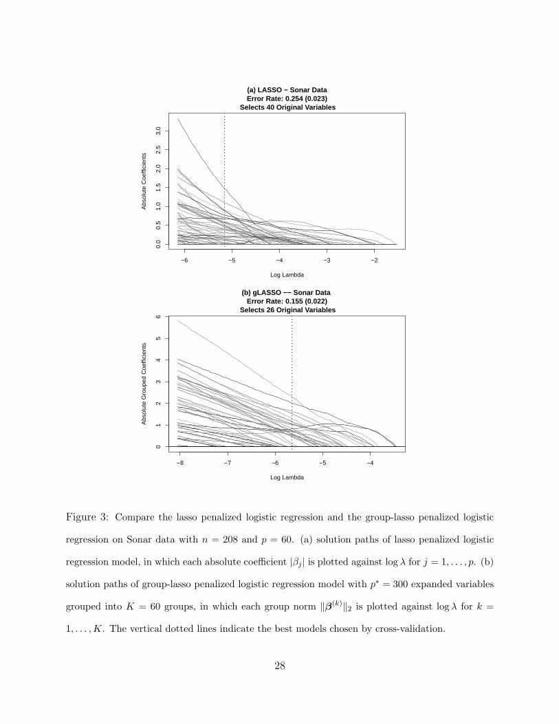
Before ending this section we would like to use a real data example to demonstrate why

the group-lasso could be advantageous over the lasso. On sonar data we compared the lasso

penalized logistic regression and the group-lasso penalized logistic regression. We randomly

split the sonar data into training and test sets according to 4:1 ratio, and found the optimal

λ for each method using five-fold cross-validation on the training data. Then we calculated

the misclassification error rate on the test set. We used glmnet (Friedman et al., 2010)

to compute the lasso penalized logistic regression. The process was repeated 100 times.

In the group-lasso model, we define the group-wise L2 coefficient norm θj(λ) for the jth

variable by θj(λ) =√∑5

i=1 β2ji(λ). Then the jth variable enters the final model if and only

if θj(λ) = 0. Figure 3 shows the solution paths of the tuned lasso and group-lasso logistic

model from one run, where in the group-lasso plot we plot θj(λ) against log λ. To make

a more direct comparison, we also plot the absolute value of each coefficient in the lasso

plot. The fitted lasso logistic regression model selected 40 original variables while the group-

lasso logistic regression model selected 26 original variables. When looking at the average

misclassification error of 100 runs, we see that the group-lasso logistic regression model is

significantly more accurate than the lasso logistic regression model. Note that the sample

size is 208 in the Sonar data, thus the misclassification error calculation is meaningful.

26

Group-lasso Regression on Real Data

Dataset Autompg Bardet Cardiomypathy Spectroscopy

Sec. — KKT Sec. — KKT Sec. — KKT Sec. — KKT

SLEP (LS) 3.14 — 0 9.96 — 0 78.23 — 0 9.37 — 0

gglasso (LS1) 1.79 — 1 8.49 — 1 0.38 — 2 0.50 — 0

gglasso (LS2) 1.29 — 0 1.04 — 0 2.53 — 0 2.26 — 0

Group-lasso Classification on Real Data

Dataset Colon Prostate Sonar Breast

Sec. — KKT Sec. — KKT Sec. — KKT Sec. — KKT

grplasso (Logit) 60.42 — 0 111.75 — 0 24.55 — 0 439.76 — 0

gglasso (Logit1) 1.13 — 0 3.877 — 0 1.54 — 0 9.62 — 0

SLEP (Logit) 75.31 — 0 166.91 — 0 5.49 — 0 358.75 — 0

gglasso (Logit2) 2.23 — 0 4.36 — 0 2.88 — 0 10.24 — 0

gglasso (HSVM) 1.15 — 0 3.53 — 0 0.66 — 0 9.15 — 0

gglasso (SqSVM) 1.45 — 0 3.79 — 0 1.27 — 1 9.58 — 0

Table 5: Group-lasso penalized regression and classification on real datasets. Reported numbers

are: (a) timings (in seconds), total time for 100 λ values; (b) the average number of coefficients

among p coefficients that violated the KKT condition check. Results are averaged over 10 indepen-

dent runs.

27

−6 −5 −4 −3 −2

0.0

0.5

1.0

1.5

2.0

2.5

3.0

(a) LASSO − Sonar Data Error Rate: 0.254 (0.023)

Selects 40 Original Variables

Log Lambda

Abs

olut

e C

oeffi

cien

ts

−8 −7 −6 −5 −4

01

23

45

6

(b) gLASSO −− Sonar Data Error Rate: 0.155 (0.022)

Selects 26 Original Variables

Log Lambda

Abs

olut

e G

roup

ed C

oeffi

cien

ts

Figure 3: Compare the lasso penalized logistic regression and the group-lasso penalized logistic

regression on Sonar data with n = 208 and p = 60. (a) solution paths of lasso penalized logistic

regression model, in which each absolute coefficient |βj | is plotted against log λ for j = 1, . . . , p. (b)

solution paths of group-lasso penalized logistic regression model with p∗ = 300 expanded variables

grouped into K = 60 groups, in which each group norm ∥β(k)∥2 is plotted against log λ for k =

1, . . . ,K. The vertical dotted lines indicate the best models chosen by cross-validation.

28

5 Discussion

In this paper we have derived a unified groupwise-majorizatoin-descent algorithm for com-

puting the solution paths of a class of group-lasso penalized models. We have demonstrated

the efficiency of Algorithm 1 on four group-lasso models: the group-lasso penalized least

squares, the group-lasso penalized logistic regression, the group-lasso penalized HSVM and

the group-lasso penalized SqSVM. Algorithm 1 can be readily applied to other interest-

ing group-lasso penalized models. All we need to do is to check the QM condition for the

given loss function. For that, Lemma 1 is a handy tool. We also implemented the exact

groupwise descent algorithm in which we solved the convex optimization problem defined in

(14) for each group. We used the same computational tricks to implement the exact group-

wise descent algorithm, including the strong rule, warm-start and the active set. We found

that groupwise-majorization-descent is about 10 to 15 times faster than the exact groupwise

descent algorithm. This comparison clearly shows the value of using majorization within

the groupwise descent algorithm. For the sake of brevity, we opt not to show the timing

comparison here.

grplasso is a popular R package for the group-lasso penalized logistic regression, but

the underlying algorithm is limited to twice differentiable loss functions. SLEP implements

Nesterov’s method for the group-lasso penalized least squares and logistic regression. In prin-

ciple, Nesterov’s method can be used to solve other group-lasso penalized models. For the

group-lasso penalized least squares and logistic regression cases, our package gglasso is faster

than SLEP and grplasso. Although we do not claim that groupwise-majorizatoin-descent is

superior than Nesterov’s method, the numerical evidence clearly shows the practical useful-

ness of groupwise-majorizatoin-descent.

29

Finally, we should point out that Nesterov’s method is a more general optimization

algorithm than groupwise-descent or groupwise-majorizatoin-descent. Note that groupwise-

descent or groupwise-majorizatoin-descent can only work for groupwise separable penalty

functions in general. What we have shown in this paper is that a more general algorithm

like Nesterov’s method can be slower than a specific algorithm like GMD for a given set of

problems. The same message was reported in a comparison done by Tibshirani in which

the coordinate descent algorithm was shown to outperform Nesterov’s method for the lasso

regression. See https://statweb.stanford.edu/∼tibs/comparison.txt for more details.

Acknowledgements

The authors thank the editor, an associate editor and two referees for their helpful comments

and suggestions. This work is supported in part by NSF Grant DMS-08-46068.

Appendix: proofs

Proof of Lemma 1. Part (1). For any β and β∗, write β − β∗ = V and define g(t) =

L(β∗ + tV | D) so that

g(0) = L(β∗ | D), g(1) = L(β | D).

By the mean value theorem, ∃ a ∈ (0, 1) such that

g(1) = g(0) + g′(a) = g(0) + g′(0) + [g′(a)− g′(0)]. (25)

Write Φ′f = ∂Φ(y,f)

∂f. Note that

g′(t) =1

n

n∑i=1

τiΦ′f (yi,x

T

i (β∗ + tV ))(xT

iV ). (26)

30

Thus g′(0) = (β − β∗)T∇L(β∗|D). Moreover, from (26) we have

|g′(a)− g′(0)| = | 1n

n∑i=1

τi[Φ′f (yi,x

T

i (β∗ + aV ))− Φ′

f (yi,xT

iβ∗)](xT

iV )|

≤ 1

n

n∑i=1

τi|Φ′f (yi,x

T

i (β∗ + aV ))− Φ′

f (yi,xT

iβ∗)||xT

iV |

≤ 1

n

n∑i=1

Cτi|xT

i aV ||xT

iV | (27)

≤ 1

n

n∑i=1

Cτi∥xT

iV ∥22

=C

nV T[XTΓX]V, (28)

where in (27) we have used the inequality |Φ′(y, f1)− Φ′(y, f2)| ≤ C|f1 − f2|. Plugging (28)

into (25) we have

L(β | D) ≤ L(β∗ | D) + (β − β∗)T∇L(β∗|D) +1

2(β − β∗)TH(β − β∗),

with H = 2CnXTΓX.

Part (2). Write Φ′′f = ∂Φ2(y,f)

∂f2 . By Taylor’s expansion, ∃ b ∈ (0, 1) such that

g(1) = g(0) + g′(0) + g′′(b). (29)

Note that

g′′(b) =1

n

n∑i=1

τiΦ′′f (yi,x

T

i (β∗ + bV ))(xT

iV )2 ≤ 1

n

n∑i=1

C2τi(xT

iV )2, (30)

where we have used the inequality Φ′′f ≤ C2. Plugging (30) into (29) we have

L(β | D) ≤ L(β∗ | D) + (β − β∗)T∇L(β∗|D) +1

2(β − β∗)TH(β − β∗),

with H = C2

nXTΓX.

31

References

Alon, U., Barkai, N., Notterman, D., Gish, K., Ybarra, S., Mack, D. and Levine, A. (1999),

‘Broad patterns of gene expression revealed by clustering analysis of tumor and normal

colon tissues probed by oligonucleotide arrays’, Proceedings of the National Academy of

Sciences 96(12), 6745.

Daubechies, I., Defrise, M. and De Mol, C. (2004), ‘An iterative thresholding algorithm for

linear inverse problems with a sparsity constraint’, Communications on Pure and Applied

Mathematics, 57, 1413–1457.

Efron, B., Hastie, T., Johnstone, I. and Tibshirani, R. (2004), ‘Least angle regression’, Annals

of statistics 32(2), 407–451.

Friedman, J., Hastie, T. and Tibshirani, R. (2010), ‘Regularized paths for generalized linear

models via coordinate descent’, Journal of Statistical Software 33, 1–22.

Fu, W. (1998), ‘Penalized regressions: the bridge versus the lasso’, Journal of Computational

and Graphical Statistics 7(3), 397–416.

Genkin, A., Lewis, D. and Madigan, D. (2007), ‘Large-scale Bayesian logistic regression for

text categorization’, Technometrics 49(3), 291–304.

Gorman, R. and Sejnowski, T. (1988), ‘Analysis of hidden units in a layered network trained

to classify sonar targets’, Neural networks 1(1), 75–89.

Graham, K., de Las Morenas, A., Tripathi, A., King, C., Kavanah, M., Mendez, J., Stone, M.,

Slama, J., Miller, M., Antoine, G. et al. (2010), ‘Gene expression in histologically normal

32

epithelium from breast cancer patients and from cancer-free prophylactic mastectomy

patients shares a similar profile’, British journal of cancer 102(8), 1284–1293.

Hunter, D. and Lange, K. (2004), ‘A tutorial on MM algorithms’, The American Statistician

58(1), 30–37.

Lange, K., Hunter, D. and Yang, I. (2000), ‘Optimization transfer using sur- rogate objective

functions (with discussion)’, Journal of Computational and Graphical Statistics 9, 1–20.

Liu, J., Ji, S. and Ye, J. (2009), SLEP: Sparse Learning with Efficient Projections, Arizona

State University.

URL: http: // www. public. asu. edu/ ~ jye02/ Software/ SLEP

Meier, L., van de Geer, S. and Buhlmann, P. (2008), ‘The group lasso for logistic regression’,

Journal of the Royal Statistical Society, Series B 70, 53–71.

Nesterov, Y. (2004), ‘Introductory lectures on convex optimization: A basic course’, Opera-

tions Research .

Nesterov, Y. (2007), Gradient methods for minimizing composite objective function, Techni-

cal report, Technical Report, Center for Operations Research and Econometrics (CORE),

Catholic University of Louvain (UCL).

Osborne, M., Presnell, B. and Turlach, B. (2000), ‘A new approach to variable selection in

least squares problems’, IMA Journal of Numerical Analysis 20(3), 389–403.

Quinlan, J. (1993), Combining instance-based and model-based learning, in ‘Proceedings of

the Tenth International Conference on Machine Learning’, pp. 236–243.

33

Sæbø, S., Almøy, T., Aarøe, J. and Aastveit, A. (2008), ‘St-pls: a multi-directional nearest

shrunken centroid type classifier via pls’, Journal of Chemometrics 22(1), 54–62.

Scheetz, T., Kim, K., Swiderski, R., Philp, A., Braun, T., Knudtson, K., Dorrance, A.,

DiBona, G., Huang, J., Casavant, T. et al. (2006), ‘Regulation of gene expression in the

mammalian eye and its relevance to eye disease’, Proceedings of the National Academy of

Sciences 103(39), 14429–14434.

Segal, M., Dahlquist, K. and Conklin, B. (2003), ‘Regression approaches for microarray data

analysis’, Journal of Computational Biology 10(6), 961–980.

Singh, D., Febbo, P., Ross, K., Jackson, D., Manola, J., Ladd, C., Tamayo, P., Renshaw,

A., D’Amico, A., Richie, J. et al. (2002), ‘Gene expression correlates of clinical prostate

cancer behavior’, Cancer cell 1(2), 203–209.

Tibshirani, R. (1996), ‘Regression shrinkage and selection via the lasso’, Journal of the Royal

Statistical Society, Series B. 58, 267–288.

Tibshirani, R., Bien, J., Friedman, J., Hastie, T., Simon, N., Taylor, J. and Tibshirani, R.

(2012), ‘Strong rules for discarding predictors in lasso-type problems’, Journal of the Royal

Statistical Society: Series B 74, 245–266.

Tseng, P. (2001), ‘Convergence of a block coordinate descent method for nondifferentiable

minimization’, Journal of Optimization Theory and Applications 109(3), 475–494.

Vogt, J. and Roth, V. (2012), A complete analysis of the l1,p group-lasso, in ‘Proceedings of

the 29th International Conference on Machine Learning (ICML-12)’, ICML 2012, Omni-

press, pp. 185–192.

34

Wang, H. and Leng, C. (2008), ‘A note on adaptive group lasso’, Computational Statistics

and Data Analysis 52, 5277–5286.

Wang, L., Zhu, J. and Zou, H. (2008), ‘Hybrid huberized support vector machines for mi-

croarray classification and gene selection’, Bioinformatics 24, 412–419.

Wu, T. and Lange, K. (2008), ‘Coordinate descent algorithms for lasso penalized regression’,

The Annals of Applied Statistics 2, 224–244.

Wu, T. and Lange, K. (2010), ‘The MM alternative to EM’, Statistical Science 4, 492–505.

Yuan, M. and Lin, Y. (2006), ‘Model selection and estimation in regression with grouped

variables’, Journal of the Royal Statistical Society, Series B 68, 49–67.

Zhang, T. (2004), ‘Statistical behavior and consistency of classification methods based on

convex risk minimization’, Annals of Statistics 32, 56–85.

Zou, H. (2006), ‘The adaptive lasso and its oracle properties’, Journal of the American

Statistical Association 101, 1418–1429.

35